AD-A266 718AF T/ E/ N /9 J-3D T I C
S ELECTEJUL 819931
C
DEVELOPMENT OF AN AIR-TO-AIR REFUELINGAUTOMATIC FLIGHT CONTROL SYSTEM USING
QUANTITATIVE FEEDBACK THEORY
THESIS
Dennis W. TrosenCaptain, USAF
AFIT/GE/ENG/93J-03
93-15348
.0. 7 08 002 I I I I I IIII , II
Approved for public release; distiibution unlimited

AFIIT/GE/ENG/93I-03
DEVELOPMENT OF AN AIR-TO-AIR REFUELING
AUTOMATIC FLIGHT CONTROL SYSTEM USING
QUANTITATIVE FEEDBACK THEORY
THESIS
Presented to the Faculty of the School of Engineering
of the Air Force Institute of Technology
Air University
In Partial Fulfillment of the
Requirements for the Degree of
Master of Science in Electrical Engineering
Dennis W Trosen, B.S.E.E.
Captain, USAF
Acce-,iuy' cr
,1993 DTIC TAb UJune, 193 av no..mccd [
Dist ibut ion I
Avdd ibility Codes
Approved for public release, distribution unlimited i Avail a-idof
Dist Specia
IA

Acknowledgements
I send thanks to my parents, Patricia and Kenneth Trosen, for shaping me into the man
I am today.
Prof Houpis and Prof Pachter, thank you for the knowledge to accomplish this thesis.
Kevin and Sean . you waited patiently for me, I love you and "daddy's all studied".
I dedicate this work to my wife, Chris whose love and understanding provides my
mctivation, you make my life whole, I love you very much.
Dennis W. Trosen
ii

Table of Contents
Acknowledgemnents..............................................ui
Table of Contents..............................................1iii
List of Piguc ................................................ Vill
List of Tables................................................. xi
Abstract..................................................... xii
I. Introduction............................................... 1-1
1.1 Background........................................... 1-1
1.2 Problem Statement...................... ............... 1-2
1.3 Assumptions......................................... 1-3
1.4 Research Objectives..................................... 1-3
1.5 Scop,. .............................................. 1-4
1.6 Methodology........................................ 1-4
1.7 Overview of the Thesis................................. 1.5
1.8 Summary........................................... 1-5

HI. QFT and Output Disturbance Rejection............................ n-1
2.1 Intruduction .. .. .. .. .. .. .. .. .. .. .. .. .. .. .. .. .. .. .. .. 2-1
2.2 Overview of QFT. .. .. .. .. .. .. .. .. .. .. ... .. .. ... .. ... 2-1
2.3 MIMO, QFT .. .. .. .. .. .. .. .. .. .. .. ... .. .. .. ... .. .. .. 2-3
2.4 MIMO QFT with External Output Disturbance .................. 2-5
2.5 Summary . ... ........................... 2-14
111. Air-to-Air Refueling FCS Design Concept.......................... 3-1
3.1 Introduction.......................................... 3-1
3.2 C-13511 Modeling...................................... 3-1
3.3 Disturbance Modeling................................... 3-4
3.3.1 Pitch Plane Wind Induced Disturbance................. 3-4
3.3.2 Lateral Channel Wind Induced Disturbance.............. 3-8
3.3.3 Disturbance Due to Refueling .... . . . . . . . . 3-8
3.4 Plant and Disturbance Matrices . . . . . . . . . . . .. 3-10
3.5 Controil Problem Approach .. . . . . . . . . . . . . . 3-11
3.6 Summary........................................... 3-15
IV. LTI Plant and Disturbance Model Generation....................... 4-1
4,1 Introduction.......................................... 4-1
4.2 Plant Transfer Function Generation.......................... 4-1
4.3 Disturbance Transfer Function Generation..................... 4-5
iv

4.4 Summary . . . . .. . . . . . . . . . . . . . .. 4-8
V. QFT AFCS Design......................................... 5-1
5.1 Introduction.......................................... 5-1
5.2 Disturbance Rejection Specification......................... 5-1
5.3 Loop Shaping......................................... 5-3
5.3.1 Channel 2 Loop Design........................... 5-3
5.3.2 Channel I Loop Design........................... 5-7
5.3.3 Channel 3 Loop Design.......................... 5-11
5.4 Closed Loop Lm Plots.................................. 5-14
5.5 Summary.......................................... 5-15
VI. Air-to-Air Refueling Simulations................................6-1
6.1 Introduction......................................... 6-1
6.2 Linear Simulations.................................... 6-1
6.3 Nonlinear Simulations.................................. 6-2
6.4 Summary........................................... 6-3
Vfl. Conclusions and Recomnieidation ............................... 7-1
7.1 Discussion.......................................... 7-1
7.2 Conclusions......................................... 7-2
7.3 Recommendations..................................... 7-2
V

Appendix A. C-135 Nondimensional Stability Derivatives ................ A-i
A.i Nondimetnsional Stability Derivative Definitions .............. A-i
A .1.1 Looitlldin41. ................................. A -I
A .1.2 Lonitudinal ................................. A -i
Appendix B. Plant Transfer Functions ............................. B-I
B.1 Plant Case 1 - C1 , = 0.2 Gross Weight = 160,666 pounds ........ B-i
B.2 Plant Case 2 - CL = 0.6 Gross Weight = 160.666 pounds ........ B-I
B.3 Plant Case 3 - CL = 0.2 Gross Weight = 207,316 pounds ........ B-2
B.4 Plant Case 4 - C1, = 0.6 Gross Weight = 207,316 pounds ........ B-3
B.5 Plant Case S - C1 = 0.2 Gross Weight = 210,189 pounds ........ B-4
B.6 Plant Case 6 - CL = 0.6 Gross Weight = 210,189 pounds ........ B-4
13.7 Plant Case 7 - CL = 0.2 Gross Weight = 245,500 pounds ........ B-5
B8 Plant Case 8 - CL = 0.6, Gross Weight 245,500 pounds ........ B-6
B.9 Plant Case 9 - CL - 0.2, Gross Weight = 253,500 pounds ....... B-6
B.10 Plant Case 10 - CL = 0.6, Gross Weight = 253,500 pounds ...... B-7
B.11 Plant Case II - CL = 0.2, Gross Weight = 263,500 pounds ...... B-8
B.12 Plant Case 12 - CL = 0.6, Gross Weight = 263,500 pounds ...... B-8
B.13 Plant Case 13 - CL = 0.2, Gross Weight = 275,500 pounds ...... B-9
B.14 Plant Case 14 - CL = 0.6, Gross Weight = 275,500 pounds ..... B-10
B.15 Plant Case 15 - C1 = 0.2, Gross Weight = 277,500 pounds ..... B-10
B.16 Plant Case 16 - C1, = 0.6, Gross Weight =- 277,500 pounds ..... B-1I
Vi

Appendix C. C-135B and Autopilot Input Response...................... C-1
Appendix D. C-135B and Autopilot Disturbance Response.................. D-1
Appendix E. Templates and Boundary Plots...........................E-1
Appendix F. QFT Conmpenisators................................... F-I
F.1 Channel 11 compensator, g,............................... F- I
F.2 Channel 2 compensator, :2...........................................F-i
F.3 Channel 3 compensator. 3. . . . . . . . . . . . . . . . . . . . . . . . . . . . . .. F-I
Bibliography................................................ BIB-i1
Vita..................................................... VITA- I
vii

List of Figures
Figure 2.1 QFT Controller Design ................................ 2-2
Figure 2.2 3x3 MISO Equivalent Loops ............................ 2-4
Figure 2.3 QFT Controller with Output External Disturbance .............. 2-6
Figure 2.4 3x3 MISO Equivalent Loops for External Output Disturbance ..... 2-9
Figure 3.1. Bare Aircraft Plant .................................. 3-2
Figure 3.2 C-135B Bare Aircraft with Autopilot ...................... 3-4
Figure 3.3 Control Problem Geometry ............................ 3-13
Figure 3.4. Control Problem . ................................... 3-14
Figure 4.1 P(s) Log M agnitude Plot ............................... 4-3
Figure 4.2 Q',s) Log M agnitude Plots .............................. 4-5
Figure 4.3 P,(s) Log M agnitude Plots .............................. 4-7
Figure 5.1 Disturbance Rejection Model Response to 10 ft/sec Impulse ....... 5-2
Figure 5.2 Channel 2 Loop Shaping P. = Plant Case 2 .................. 5-5
Figure 5.3 Channel 2 Nichols Plot all Plant Cases ..................... 5-6
Figure 5.4 Channel 1 Loop Shaping P,, = Plant Case 2 .................. 5-9
Figure 5.5 Channel 1 Nichols Plot all Plant Cases .................... 5-10
Figure 5.6 Channel 3 Loop Shaping P. = Plant Case 2 ................. 5-12
Figure 5.7 Channel 3 Nichols Plot all Plant Cases .................... 5-13
Figure 5.8 MISO Equivalent System Lm Plots ...................... 5-14
Figure 6.1 Linear Simulation - Z Separation Deflection all Plant Cases ....... 6-4
viii

Figure 6.2 Linear Simulation - X Position Deflection all Plant Cases 6-5
Figure 6.3 Linear Simulation - Y Position Deflection all Plant Cases ........ 6-6
Figure 6.4 Nonlinear Simulation - X, Y, Z Position Defection, Plant 1 C, =
0 .2 . . . . . . . . . . . . . . . . . . . . . . . . . . . . . . . . . . . . . . . . . . . . . . . . . 6 -7
Figure 6.5 Nonlinear Simulation - Control Surface and Throttle Response,
Plant 1............................. ................. 6-8
Figure 6.6 Nonlinear Simulation - X, Y, Z Position Deflection, Plant 2 CL =
0 .6 . . . . . . . . . . . . . . . . . . . . . . . . . . . . . . . . . . . . . . . . . . . . . . . . . 6 -9
Figure 6.7 Nonlinear Simulation - Control Surface and Throttle Response,
Plant 2 .. ............................................. 6-10
Figure C.1 Mach Hold Response to 1 ft/sec Step Input - CL = 0.2 .......... C-2
Figure C.2 Mach Hold Response to 1 ft/sec Step Input - CL = 0.6 .......... C-3
Figure C.3 Altitude Hold Response to 1 foot Step input - CL = 0.2 .......... C-4
Figure C.4 Altitude Hold Response to 1 Foot Step Input - C = 0.6 ......... C-5
Figure C.5 Rudder Control Response to 1 deg Step Input - CL. = 0.2 ......... C-6
Figure C.6 Rudder Control Response to 1 deg Step Input - CL = 0.6 ......... C-7
Figuie C.7 Aileron Controi Response to 1 deg Step input - CL = 0.2 ........ C-8
Figure C.8 Aileron Control Response to 1 deg Step Input - C1. = 0.6 ........ C-9
Figure D.1 X, Y, Z Response to Longitudinal Wind Disturbance - CL = 0.2 ... D-2
Figure D.2 X, Y, Z Response to Longitudinal Wind Disturbance - C = 0.6 ... D-3
Figure D.3 X, Y, Z Response to Lateral Wind Disturbance - CL = 0.2 ....... D-4
Figure D.4 X, Y, Z Response to Lateral Wind Disturbance - CL = 0.6 ....... D-5
ix

Figure D.5 X, Y, Z Fe,.onse to Refueling Disturbance - C = 0.2 .......... D-6
Figure D.6 X, Y, Z Response to Refueling Disturbance - C1 = 0.6 ......... D-7
Figure F.! Channel I Tem plates ................................. E-2
Figure E.2 Channel 1 Stability Bounds ............................. E-3
Figure E.3 Channel I Disturbance Bounds ....................... . E-4
Figure E.4 Channel 2 Templates ................................. E-5
Figure E.5 Channel 2 Stability Bounds ................ .......... E-6
Figure E.6 Channel 2 Disturbance Bounds ........................... E-7
Figure E.7 Channel 3 Templates ................................. E-8
Figure E.8 Channel 3 Stability Bounds ............................. E-9
Figure E.9 Channel 3 Disturbance Bounds ......................... E-10
x

List ol 'Taiblc
Table A. 1 Constanit Stability Derivatives for all Plant Cases ............. A-2
Table A.2 Stability Derivatives that Change with C,. .. . . . . . . . . . . . . . . . . . . . . A-3
Table A.3 Stability Derivatives that Change with Weight and Center of
Gravity.......................... ..................... A-3
xi

AFIT/GE/ENG/93J-03
Abstract
Quantitative Feedback Theory and the improved method Quantitative Feedback
Theory are enhanced to include the rejectioa of disturbance at the system output. The
enhanced Quantitative Feedback Theory and improved method Quantitative Feedback
Theory processes are applied to the design of an automatic flight control system to
regulate position of the C-135B fuel receiving aircraft relative to the tanker during air-to-
air refueling. A simple feedback control system is developed that will achieve stable
position regulation. State-space aircraft models are generated. An "inner loop" autopilot
is designed to reduce the plant cutoff frequency and provide the system inputs for the
Quantitative Feedback Theory compensators. Disturbance models representing disturbance
due to wind gusts and refueling are developed. The flight control system is designed
using the enhanced Quantitative Feedback Theory equations. Linear simulations are
performed on MATRIXx, and nonlinear simulations are run on EASY5x. The results of
the simuladons show excellent results. The simulation results indicate that air-to-air
automatic flight control system are technically achievable, and that implementation in
US/ F aircraft is possible.
xii

DEVELOPMENT OF AN AIR-TO-AIR REFUELING
AUTOMATIC FLIGHT CONTROL SYSTEM USING
QUANTITATIVE FEEDBACK THEORY
I. Introduction
1.1 Background
The United States Air Force (USAF) has the mission of transporting large quantities
of material and troops over great distances. To meet this requirement, the USAF
maintains a fleet of large cargo/transport aircraft. Refueling these aircraft during flight
provides unlimited range of operation for this fleet of aircraft. However, long flights and
multiple air-to-air refuelings can seriously strain and fatigue the pilot, decreasing flight
safety, and extending recovery time between missions.
Cargo/transport aircraft are generally large and have high moments of inertia.
Piloting a large, high inertia aircraft during air-to-air refueling requires intense
concentration. The pilot must maintain a very precise position relative to the tanker.
He/she maintains position visually, applying the appropriate control inputs when changes
in position occur. The pilot must compensate for changes in aircraft dynamics due to
taking on fuel, specifically, changes in center-of-gravity and moments of inertia I,, and
I4,. Besides dynamic changes. the pilot must contend with maintaining position in the
presence of wind gusts. Since these aircraft can take on large amounts of fuel, up to
250.000 pounds, air-to-air refueling can take up to 30 minutes. Compound this over long
flights and multiple refuelings, the pilot's fatigue level increases and can reach an unsafe
1-1

level, endangering the flight crew, and possibly impact USAFs capability to perform its
mission.
One way to ease the pilot workload is to implement an automatic flight control
system (AFCS) for air-to-air refueling. The AFCS needs to be able to maintain a precise
position of the fuel receiving aircraft (receiver) relative to the tanker in the presence of
such disturbances as wind gusts and mass changes. In this thesis, an AFCS is designed
to precisely regulate position relative to the tanker by applying the control synthesis
techniques of Quantitative Feedback Theory (QFT). QFT is a design technique developed
by Dr. Isaac Horowitz that quantifies the plant uncertainties and/or disturbances and uses
this information to design feedback compensation to achieve stability, robustness, and
desired system performance in the face of parametric uncertainty and disturbances [2].
For the regulation problem, a multiple-input multiple-output (MIMO) QFT design
method is developed to address the disturbances entering the system at the output. Dr.
Horowitz's original MIMO QFT development modeled all disturbances as entering the
system at the input of the plant [3]. In this thesis, MIMO QFT is expanded to account
for disturbances at the system output.
The sponsor for this thesis is the Flight Dynamics Directorate, Wright Laboratory,
Wright-Patterson AFB, OH.
1.2 Problem Statement
During air-to-air refueling, the receiver aircraft wil; change position relative to the
tanker. The pilot must pay close attention and take corrective action to maintain position.
Excessive changes in position will disconnect the boom from the receiver. An AFCS
1-2
must be designed to regulate the receiver's position, thus reducing the pilot workload and
fatigue factor. By using MIMO QFT, an AFCS is designed that operates throughout the
range of the changing aircraft dynamics and rejects disturbances including those at the
output (3].
1.3 Assumptions
The following assumptions are made for this thesis.
• Only the desired outputs are of interest for final performance.
" The robustness of the CAD packages used, MIMO/QFT, EASY5, MATRIX, andMathematica are adequate for the design process.
" Position of the receiver aircraft relative to the tanker during air-to-air refueling canbe accurately measured.
The first assumption is required in applying MIMO QFT. The second assumption
is concerned with the limits of CAD packages and their numerical robustness. The third
assumption is required because no sensors are currently in place to measure the position
of the receiver relative to the tanker.
1.4 Research Objectives
This thesis (1) develops aircraft models for the QFT design from a published
document [1] containing C-135 cargo aircraft stability derivatives tables and plots, (2)
presents a design for multi-channel control laws using MIMO QFT for several flight
conditions with special emphasis on changing aircraft center-of-gravity and weight, (3)
simulates the design for linear and nonlinear performance on MATRIX, and nonlinear
1-3
performance on EASY5x, (4) evaluates the new control law, and (5) validates the
development of MIMO QFT design with disturbances at the output.
1.5 Scope
This thesis applies the MIMO QFT technique to the design of an AFCS regulator for
the three-dimensional separation (x, y, and z) of a C-135B (receiver) cargo aircraft
relative to a tanker. The AFCS applies only to the receiver and is independent of the
tanker in as much as the tanker is used as the point of reference. MIMO QFT design
techniques are developed for disturbances at the system output. The present MIMO/QFT
CAD package [4] is modified to incorporate the output disturbance development. The
AFCS is designed to reject disturbances at the x, y, and z outputs in order to keep the
receiver aircraft in a volume specified as the area of boom operation [1]. Models are
developed for disturbances due to wind gusts and receiving fuel. The MIMO QFT plant
is the C-135B bare-aircraft model augmented by a typical Mach-hold, altitude-hold, wing-
leveler autopilot. QFT compensators control the reference signal of the autopilot to
.achieve "formation maintenance" during air-to-air refueling. The control system is
simulated for linear performance in MATRIX1 . A full six-degree-of-freedom nonlinear
simulation is performed in EASY5x.
1.6 Methodology
The design approach requires six steps:
* Generate linear time-invariant (LTI) state-space models of the C-135 for differentweights and center of gravity.
1-4

" Implement a Mach-hold, altitude-hold, wing leveler autopilot that operates for all
aircraft models.
* Model the disturbances due to wind gusts and refueling.
• Extend QFT design approach for disturbances at the output.
* Design the AFCS ting QFT.
" Simulate the design on MATRIX, and EASY5x to validate the AFCS design.
1.7 Overview of the Thesis
This thesis describes the research performed in the development of the AFCS.
Chapter 11 discusses QFT and the expansion of the QFT equations to include external
output disturbance. The air-to-air refueling AFCS concept is discussed in Chapter III.
Chapter IV presents the aircraft and disturbance models. The AFCS design process is
shown in Chapter V followed by linear and nonlinear simulations in Chapter VI. Finally,
Chapter VII presents the thesis conclusions and recommendations.
1.8 Summary
Future USAF cargo/transport requirements may very well involve long flights with
many air-to-air refuelings An AFCS to automatically pilot the aircraft during air-to-air
refueling will greatly reduce the pilot workload and reduce fatigue. MIMO QFT design
techniques are ideally suited for the design of such a flight control system with its wide
range of parameter uncertainty. This thesis takes on the challenge of validating MIMO
QFT for design of regulator AFCSs. And demonstrating automatic air-to-air refueling
flight control systems are technically achievable. The next chapter briefly reviews the
QFT process and the development of the output disturbance QFT design technique.
1-5

II. QFT and Output Disturbance Rejection
2.1 Introduction
The essence of QFT designed compensators is the ability to accommodate plant
paremeter structured uncertainty and reject disturbances [2]. This Chapter outlines the
QFT method and how nonlinear plants can be modeled as linear-time-invariant (LTI)
plants with uncertainty. First a brief description of QVI" is presented, followed by the
development of the QFT output disturbance model.
2.2 Overview of QFT
Quantitative Feedback Theory is a powerful design method for synthesizing fixed
parameter compensation capable of controlling a system in the realities of large plant
uncertainties, disturbance (rejection), nonlinear plant models, time variations of plant
parameters, and stringent performance specifications. Included in QFT is the ability to
design a compensator to cause the system to produce outputs that meet required specifica-
tions based on particular inputs and disturbance rejection requirements. The general QFT
design process is based on the diagram presented in Figure 2.1, which represents either
a multiple-input single-output (MISO) or a MIIMO system [2] [3]. U represents the
commanded input and D1, D2 are disturbance inputs. G(s) is a cascade compensator and
F(s) is a prefilter. In QFT, P(s) represents a set of J LTI transfer functions, representing
the plant at different operating conditions. The designer chooses the individual transfer
2-1

DD
U F(s) G s P(s) •
Figure 2.1 QFT ControUer Design
functions, Ps(s) E ?(s), where j=1,2,....J, so that the entire operational envelope or the
structured uncertainty of the plant is adequately covered. The prefilter, F(s), is designed
so that the system meets the tracking requirements of the output Y to the input U. For
a regulator control system (as opposed to tracking) the commanded input is zero, thus, no
prefilter is required.
The objective in designing the G(s) compensator is to ensure that the set of control
ratios (when applicable):
TR(s) Y(s) = F(s)G(s)P(s) (2.1)Ud(s) 1 + G(s)P(s)
and the disturbance ratios:
T Y(s) = P(s) when D2 =0 (2.2)D)(s) 1 + G(s)P(s)
T Y(s) = Y(s) P(s) when D, =0D2(s) 1 + G(s)P(s)
meet the desired performance and disturbance rejection specification for all Ps(s) E 9(s).
The nominal loop transmission is Lo, expressed as
2-2

Lo = GPO (2.4)
where P0 represents the nominal plant. The designer selects P0 E T(s) based on his/her
preference on the placement of the templates' boundaries. To form the stability bounds,
templates are derived based on the T information. The templates are plots of the dB
magnitude versus phase, for a fixed frequency o, for each Pi contained within TP = {Pj}.
L. is shaped to meet the tracking BR(S) and/or disturbance rejection BD(S) bounds derived
from the templates on the Nichols chart. Combining BR(s) and Bv(s) yields the optimal
boundary Bo0(O), which along with the stability contour (U-contour), constrain L. such
that for each frequency coi, the Lm L0(jco) point must lie on or above Bo(jw), and not
intersect the U-contour. Once L. is formed, G(s) is directly derived from Eq. (2.4).
After G(s) is formed, whenever applicable, the prefilter F(s) is shaped to guarantee
that the closed loop frequency response lies withir the desired tracking specifications.
In the case where Ud = 0 (regulator), the prefilter is not required and the problem
becomes a pure disturbance rejection problem . In this thesis, the rejection of the 'input
disturbance D2 at the system output is the desired performance specification.
2.3 MIMO QFT
Multiple-input multiple-output QFT design method requires transforming the system
into equivalent multiple-input single-output (MISO) loops as shown in Figure 2.2 for he
3x3 case. The Schauder fixed point Theorem justifies the sequential design process,
where each loop is individually "closed" [2]. Equation (2.5) represents the control ratio
: which relates the ih output to the P input of the ij MISO loop, where i = 1,2,...,m, and
2-3

dnl dj,fn , ! Y,1 fu2 gly / Yt2 d13 Y1
d 3
13
21 -12
f~1 9 2 d' 2 22 92 d Y1 1f23 92 d3 Y23)113U 21 22 q2 j 1123
fh, 3 ~ Y31 f32 9-d2,_3 93 d3 3
/ ~/d 32 /d 33
f31 gw U32.3 Y3'Jq 2 U33
1133331 q;2£3 1.Y32 % £3
-1-1-
Figure 2.2 3x3 MISO Equivalent Loops
j = 1,2,...,m, f is the prefilter of the ij MISO loop, 1, is the i loop transmission, and d,
represents the disturbance input in the ij loop. The q. are the reciprocal of the terms
contained in the inverse of the square plant matrix P = [p,]. That is, P" = fp' ] = P
where [PU] = [1/%], and Q = [q]. The disturbance dj given by Eq. (2.6) represents the
cross-coupling between loops. The disturbance bounds BD, are calculated to satisfy Eq
(2.7).
, (2.5)1+1
Sk 1, 2,. md -E2- (2.6)
2-4

It + I 2 .2 (2.7)
Note, external disturbances are not accounted for in this development. Only cross-
coupling loop to loop interaction type disturbances are considered. A separate MIMO
QFT development including external disturbances is presented in the following section.
According to the original QFT method each loop is designed independently, but this
leads to extreme overdesign. A better approach, called the improved method, is to utilize
the known structure of g, and f of the loop that is designed first. The improved method
uses the known structure of the designed loop to provide a more accurate estimate of the
cross-coupled disturbance from the designed loop to the other uncompensated loops.
Based on the new estimate of the cross-coupled disturbance, new disturbance rejection
bounds for the uncompensated loops are calculated. The improved method is applied after
each loop is compensated. The normal QFT loop shaping process is performed for a
given uncompensated loop using the new disturbance bounds. The improved method
reduces the overdesign of the original method by taking into account that compensated
loop will have less cross-coupling disturbance intc the uncompensated loops. [31
2.4 MIMO QFT with External Output Disturbance
Output disturbance rejection is the primary design criterion in this thesis. The
previous discussion of MIMO QFT did not consider external disturbance in the calculation
of disturbance rejection bounds. Therefore, equations including the external disturbance
are developed in this thesis. The following discussion outlines this development.
2-5
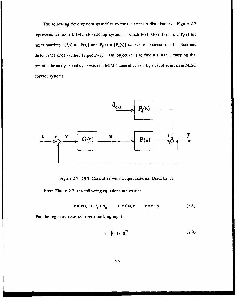
The following development quantifies external uncertain disturbances. Figure 2.3
represents an mxm MIMO closed-loop system in which F(s), G(s), P(s), and Pd(s) are
mxm matrices. P(s) = {P(s)} and rd(s) = {Pd(s)} are sets of matrices due to plant and
disturbance uncertainties respectively. The objective is to find a suitable mapping that
permits the analysis and synthesis of a MIMO control system by a set of equivalent MISO
control systems.
dext d(S)
Figure 2.3 QFT Controller with Output External Disturbance
From Figure 2.3, the following equations are written
y = P(s)u + Pd(s)d., u = G(s)v v = r- y (2.8)
For the regulator case with zero tracking input
r=[O, 0, O]T (2.9)
2-6

From Eqs. (2.8) and (2.9) where henceforth the (s) is dropped in the continuing develop-
inent
v- u Gy (2.10)
which yields
y =-PGy Pd, (2.11)
Equation (2.11) is rearranged to yield
y =[I +PG]-'Pd, (2.12)
Based upon unit impulse disturbance inputs for d,,,, the system control ratio relating d,,,
to y is
T, =[I +PGl'P, (2.13)
Premultiply Eq. (2.13) by [I + PG] yields
[I +PGJT, Pd (2.14)
when P is nonsingular. Premultiplying both sides of Eq. (2.14) by P" results in
[P-' GIT, = P-'Pd (2.15)
Let
P *11 P *12 P 'Pl P'1 * " P *,P 2 , P2 2 ... P (2.16)
P "J P ".'P
2-7

The m2 effective plant transfer functions are formed as
1 detP (2.17)
U adj PU
the Q matrix is then formed as
q,, - q, 11p,, l/P, 2 ... 1/p *I-q21 q: -. qzr / 1/ 1): l/p ..1/ 'z (.8
Q=
q,, qm2 "mm 11P 1 ) %n .. 1P m
where P = [p P" = L.,] - [l/q4q, and Q = [q0] = [1/p'j. Partition the P" matrix as
follows;
P =[pj 1 = lq, I = A +B (2.19)
where A is the diagonal part of P" and B is the balance of P'. Thus .. = I/q, = p',,, bu
= 0, and b, = 1/qv =p% for i *j. Substituting Eq. (2.19) into Eq. (2.15) with G diagonal,
results in
[A +B + IT, [A +B ]P, (2.20)
Rearranging Eq. (2.20) produces
Td =[ A +G [ Bpd -BTdI (2.21)
This equation defines the desired fixed point mapping, where each of the m2 matrix
elements on the right side of Eq. (2,21) are interpreted as MISO problems. Proof of the
fact that the design of each MISO system yields a satisfactory MIMO design is based on
2-8

del/ de1 2 dc 3911j 9 j 'Yd£1 -- q " - 13
de2 den d,2
g2 £ 92 -
21 21 ii 2
/de3t de 32; d e33
93 Ydg 3 Y 3q 3
1 q, 7 32 qII 33
Figure 2.4 3x3 MISO Equivalent Loops for External Output Disturbance
the Schauder fixed point theorem. [2] The theorem defines a mapping Y(Td)
Y(Td) =[ A +G ]'[ APd +BP d -BTd ] (2.22)
where each member of Td is from the acceptable set Sd. If this mapping has a fixed point,
i.e., T, E 3d, then this Td is a solution of Eq. (2.21).
Figure 2.4 shows the effective MISO loops resulting from a 3x3 system. Since A and
G in Eq. (2.21) are diagonal, the (1,1) element on the right side of Eq. (2.22) for the 3x3
case, for a unit impulse input, provides the output
2-9

_ q11 Pd, Pd, Pd,. td, trd, (2.23)
Y,, 1 + gqq q-'* q2 q 13 ql12 q 13
Equation (2.23) corresponds precisely to the first structure in Figure 2.4. Similarly,
each of the nine structures in Figure 2.4 corresponds to one of the elements of Y(Td) of
Eq. (2.22). The control ratios for the external disturbance inputs d,,, and the correspond-
ing outputs y, for each feedback loop of Eq. (2.22) have the form
y. = w( d, ) (2.24)
where w,, = qJ(1 + gjqj) and
P _ d. td x = number of disturbance inputs (2.25)1 -I k", q m = dimension of square MfIMO system
Thus Eq (2.25) not only contains the loop interaction but also the external disturbances.
Additional equations, quantifying the internal cross-coupling due to external
disturbances, are derived to utilize the improved method QFT design technique. These
equations are used to define the disturbance bounds for subsequent loops based on the
completed design of a single loop. For this development, the equations for the case of
a 2x2 MIMO :system are presented.
From Eq. (2.24) and for the 1-2 loop case, which is the output of loop 1 due to
disturbance input 2, including the cross-coupling terms from loop 2, yields, for unit
impulse inputs, the following control ratio
2-10
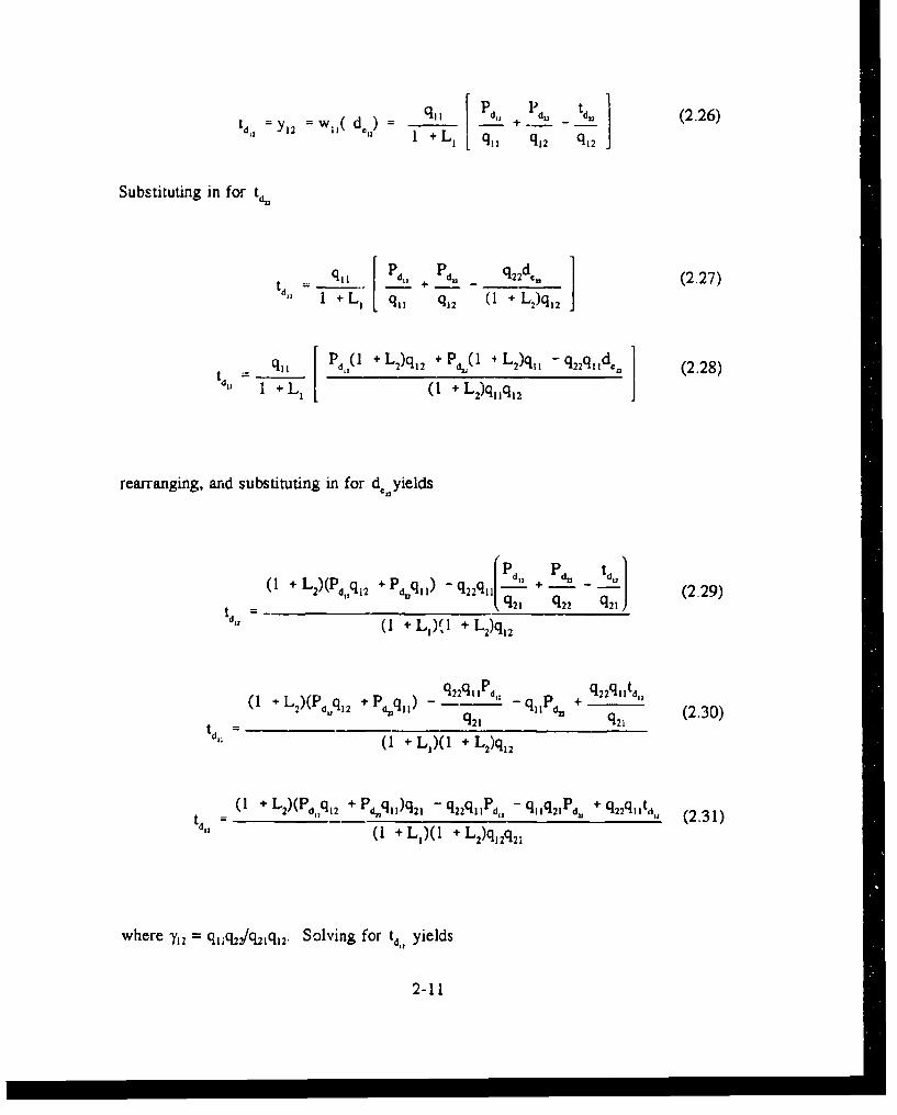
Pd 12 tw,( d..) = _ [_ (2.26)1 +L q11 q12 q12
Substituting in for tan
Pd. Pd. qd22 d,, (2.27)d 1 + L I q- q12 (1 + L2)q 2
_ qII [ Pd;, ( 1 + L2)q1 2 + Pd. ( I + L2)qll - q22qld 1 (2.28)
+ 1 [ (1 + L2)q1q 2
rearranging, and substituting in for d, yields
(1 + L2)(Pdq 2 + Pdq q ) - q-2qI _ +L _ (2.29)
t, d " (1 + L )(1 + L2)q12
(I + L )(P q 2 + P 2q ) -qIPd, + q2( 3td, q 21 q 21 (2301 (I + L)(I + L)q12
t (1 + L2)(Pdq 12 + P dq,)q 21 - q22qJIPd, - qI1q21Pd. + q22qltd,, (2.31)d" = (I + LI)(l + L2)q1 2q22
where 7,2 = qlq 2/hq21 ql2. Solving for td, yields
2-11

(I + LJ)(P d, 12 12 Pd ql )td,((l+ L +)(I L 2)) = ( L 2 (3.32)
q I ,2 _ 7 12 p , 2 + Y 2 t d ,
q 12
td,((1 + L,)(l + L2) - Y12) =
(I + L2)Pq1I ( L)P - q P (333))q q12 d 12Pdz,
LqP (1 + L, - Y )Pd (334)
t dl LI(1 +L 2) +1 +L2 -7 1 2
Equation (3.34) is rearranged as follows:
L2 q1IP d,q 12 _ _ + P
( . 51 +L2 -y2 (3.35)
1+ L,(1 + L2)1 +L2 -Y 2
From Eq. (3.35) the effective plant is defined as
q11. a qI1(1 +L 2) (3.36)
1 +L2 -Y 12
Substituting Eq. (3.36) into Eq. (3.35), yields
Thus, in general, for the 2x2 case, the improved method control ratio of the P
external disturbance input to the 1' system output is
2-12

LPdq it.+ Ptd q 12(l + L 2) + a ' (3.37)
1 + glqI.
L ~ ~ I . -+ P d (3 .3 8 )td q,,(1 + Lk) there i = 1, 2 and k * ita (1 + g.
The new disturbance bounds are calculated at a given frequency to satisfy
Lk P q" + Pa d(3.39)
t. qa(1 + Lk).I>t .I = q
_(1 L _ where i = 1, 2 and k # i
S+gq..
or
I1 + gf" d, q>, +- LPP(3.40)
1 Bl q(I +L k) where i =1, 2 and k * i (3.40)
The improved QFT method uses these equations to reduce overdesign inherent in the
original design process. The order in which loops are designed is important. Any order
can be used, but some orders produce less overdesign (less bandwidth) than others. The
last loop designed has the least amount of overdesign, therefore the most constrained loop
is done first by the original method. Then the design is continued through the remaining
loop by the second method. The first loop is then redesigned using the improved method.
At this point it is important to point out that when the disturbance rejection
specification is considered, the designer must decide how much disturbance rejection is
2-13

for cross-coupling and how much is for external disturbances. In other words the designer
can "tune" the disturbance rejection specification depending on the nature of the
disturbance for a particular loop. For example, if one loop is only effected by external
distrubance, the disturbance rejection specification would consider external disturbance
only. But if the loop disturbance was a mix of cross-coupling and external disturbance,
the designer would have to "tune" the disturbance rejection specification accordingly.
Since each loop may not exhibit the same disturbance characterisitics, disturbance
rejection specification tuning provides flexibilty in the QFT design process.
2.5 Summary
This chapter presented the basic improved QFT method and its extension to MIMO
systems. The development to include the effects of external output disturbances is
detailed. Equations to calculate the new disturbance bounds for the improved method are
discussed. The next chapter covers modeling the aircraft and the external disturbances.
2-14

III. Air-to-Air Refueling FCS Design Concept
3.1 Introduction
The aircraft modeled in this thesis is the cargo variant of the 135 class aircraft, the
C-135B. This aircraft is chosen because of the availability of the aerodynamic data [1].
This chapter describes the modeling of the C-135B. A Mach-hold, altitude hold, and
wing-leveler autopilot is included in the C-135B model [6]. Wind gusts and fuel transfer
disturbance models are developed in this chapter, as well as the AFCS concept.
3.2 C-135B Modeling
EASY5x is used to develop the state-space six-degrees-of-freedom bare (uncontrolled)
aircraft model. EASY5x is a computer aided design (CAD) tool, written by Boeing
Computer Services, used to model, simulate, and analyze dynamic systems [5]_ EASY5x's
graphical interface expedites modeling and analysis. Generic pre-written air vehicle
modules further simplify modeling in EASY5x. The user need only provide aircraft
stability derivatives, flight conditions, and desired input/outputs.
The basic aircraft model is illustrated in Figure 3.1. The LO block calculates the
longitudinal forces and moments, while LD does the same for the lateral-directional axes.
The AV block includes the aerodynamic variables and calculates changes in speed and
rates due to wind gusts. Also, it computes dynamic pressure and angle-of-attack (AOA).
The SD block contains the six-degrees-of-freedom equations of motion. It calculates
3-1

~LO
Rda LD SD
Figure 3.1. Bare Aircraft Plant
attitude, body axes rates, Euler angles, and body axes angular rates based on data supplied
by the LO and LD blocks. Further information can be obtaired from the EASY5x user
manual [5].
Sixteen bare aircraft plants are developed to account for the uncertainty of the C-
135B during air-to-air refueling. The 16 models are based on two different coefficients
of lift, CL = 0.2, 0.6, for eight different aircraft weights, each flying Mach 0.69 at 28,500
feet. These discrete values are selected based on the availability of data, normal refueling
speed and altitude, and represent weights ranging from empty/low fuel to loaded/full fuel
aircraft. Typically, during air-to-air refueling, the C-135B will have a C, between 0.27
and 0.45 [I]. Therefore, the 16 plant models envelop the structured uncertainty of the C-
3-2

135B during air-to-air refueling. Tables containing the aerodynamic stability derivatives
for all 16 plant models are provided in Appendix A.
The six-degrees-of-freedom state-space models, generated by EASY5x, are loaded
into MATRIX. MATRIXD is a programmable, matrix calculator with graphics.
MATRLX. was designed by control engineers to aid in the design of complex control
problems. It is ideally suited to manipulate matrices and apply both input/output
(classical) control and state-space (modern) control [7].
MATRIX, is used to design the autopilot using root-locus design techniques. The
autopilot is designed to control all 16 plant cases. The bare aircraft and autopilot are
shown in Figure 3.2. An autopilot is used for two reasons: (1) autopilots reduce the high
frequency cutoff of the aircraft (2) all aircraft have autopilots. Lowering the cutoff of the
aircraft reduces high frequency parameter uncertainty. Since autopilots are available,
using it in the QFT design eliminates duplication of a control system to provide input to
the bare aircraft, reducing cost and overhead. The inputs to the autopilot are thrust,
elevator, aileron, and rudder commands. The outputs are z-position (altitude), x-position,
and y-position in a local inertial reference frame where x is positive out the nose of the
aircraft, y out the right wing, and altitude is positive up. The three outputs frame of
reference is translated from the aircraft center of gravity (cg) to the approximate location
of the air-to-air refueling receptacle on the top of the aircraft.
In order to have a square plant, 3x3, one of the autopilot inputs is not used. The
Mach hold command input is used to control the x position, altitude hold controls altitude,
and the rudder command is used to control the y position. Mach and altitude are self
3-3

A~~~ ~~~ lttd dZ I t
Figure 3.2 C-135B Bare Aircraft with Autopilot
evident, rudder is chosen over aileron because the rudder does not roll the aircraft as
much as the ailerons. By using the rudder for the QFT controller, good performance is
obtained while leaving the aileron controller to handle wing leveling. See Appendix C
for aircraft response to step input commands on all four autopilot command inputs.
3.3 Disturbance Modeling
Disturbance models are generated by developing augmented state-space models of the
aircraft in the presence of wind gusts and fuel transfer inputs. This development starts
by examining the aerodynamic moments and forces.
3.3.1 Pitch Plane Wind Induced Disturbance
In the pitch plane, the total aircraft airspeed is a combination of wind velocity
and aircraft velocity in the x and z stability axis directions.
3-4

Aiipeed _ - (3.1)W A W + W I
Where ID is the steady-state aircraft speed, u & w are the perturbation speed in the
x and z directions respectively, and u,, & w,,. are the aircraft speeds due to wind in the
respective x and z directions.
The pitch plane aerodynamic moments and forces are in the form of the following
functions
M - lSc (a q, 180)
F1 -_S C (a, 8) (3.2)m
F !_ C(x, q, 6)(i)M U1 71
where
q lP (UA2 + WA2)
x arctan [W]_WA (33)
and the ex effects in the M and F, equations are neglected.
It is important to note that the following equations of motion are written with respect
to the inertial kinematic variables q. U, and W. However, the perturbations in U and W
are u + u,, and w + w, respectively. The q perturbation is q + q,.
3-5

The 4 equation of motion is
4 =MQa + Mqq + Mqq. + Mb5
+ l8 OPSC C[U(U + U-) + WA(W + W1)] Mt iW(3.4)
=MQa + Mqq + Mqqw. +M 6 8
+ 180 pSEC(O+u + u,,)(u + U) +(w + w)]+ M w.It I rJ
assuming u, w, u, and w,, << 0 Eq. (3.4) reduces to
41 Mq - Mqq,, + Mbb + M,[u + u,.] + M.1lw (3.5)
grouping the wind terms results in
l = M t+M q+M65 u Mu+ [Mqq.+ M.u,,+M w (36)
A similar derivation for the & and 6i equations of motion yield
d =Z a+Zqq+Zu+Z66+ [Z.u +(Zq l)q,.+ 1 dw,, -IZU dt (3.7)
6l = aa + Xqq + X+u + X, + [Xw. + Xqqw + 1XYw ]
Hence, the effect of a moving airmass is akin to "process noise", i.e., if the state is
x u, cc, q) (3.8)
3-6

the state-space equation
i= Ax + Bu (3.9)
is augmented to yield
i =Ax +Bu 'pithd (3.10)
where
0 0 0X U X 1X
X Xq 24
r z z -1 (3.11)0 "
M, M IM
and the disturbance vector is
d =,,h q,, (3.12)
wW
1 dwwNote, -j , which is an angle-of-attack rate, is neglected. This simplification is in
line with discarding of the i effects. Further simplification is achieved by neglecting
q,,. Hence, Fp, and dPj,,h in the pitch channel are reduced to
3-7

0 0
x -x
X 1X
0 , W
3.3.2 Lateral Channel Wind Induced Disturbance
For the lateral channel, arguments similar to the pitch channel development are
made to generate the augmented state-space equation for the effects of wind. In
conformity with the level of modeling in the pitch channel, if the state is
x = (Y, p, r, 13) (3.14)
1-w and d. are derived to be
0
1L"0
', IN d. [v (3.15)
1yY
3.3.3 Disturbance Due to Refueling
As the aircraft is taking on fuel, the moments of inertia and cg are changing.
These variations alter the flying behavior of the aircraft. This change in aircraft behavior
3-8

is modeled as a disturbance. Based on first order approximation, refueling (rf) caused
disturbance is confined to the pitch channel. Again, paralleling the pitch channel
development, the state-space model is augmented. Ft and df are found to be
0
0
12 1 32.2 d,, =[fuel transfer rate (lbs/min)] (3.16)
100 iy)1 32.2-ID I
t '
Where 12/100 is the percentage of the mean aerodynamic cord the cg is allowed to shift
during refueling and mn is the mass of the aircraft.
3.3.4 Total Disturbance
The total modeled disturbance is
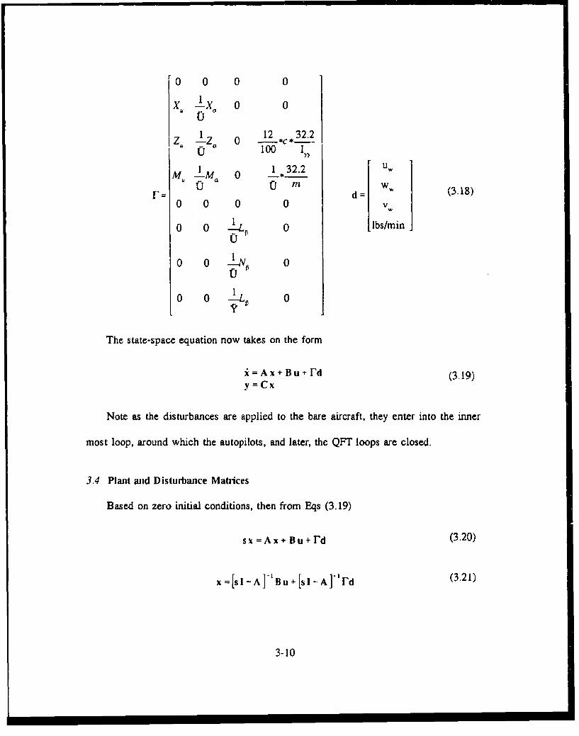
Id=r d + r.,d, + rd (3.17)
where Fr,,h and rF augment the state-space equation containing the states that identify
pitch plane flight behavior. In the same manner, F,. augments the lateral channel states.
The result of the disturbance summation for the augmented disturbed states (0, u, a, q,
W, p, r, ) is shown in Eq. (3.18).
3-9
0 0 0 0
X- X 0 0u0a
z 1 Z 0 12 32.2
U 100 In
M I. 0 1* 32.2
F u 1 m (3.18)0 0 0 0 v
0 0 0 lbs/minU
0 0 -IO 0
0 0 -IL 0
The state-space equation now takes on the form
i= Ax + Bu + Id (3.19)y =Cx
Note as the disturbances are applied to the bare aircraft, they enter into the inner
most loop, around which the autopilots, and later, the QFT loops are closed.
3.4 Plant and Disturbance Matrices
Based on zero initial conditions, then from Eqs (3.19)
sx =Ax+ Bu +rd (3.20)
x =[sl-A ]-'B + [sl-A]-31d (3.21)
3-1

y =Cx =C[sI-A]-'Bu + C[s I -AI'd (3.22)
= P(s)u + Pd(S)d
where
P(s) = C[sI -A ]-'B (3.23)
Pd(s) =CISI -A]-'T
Equation (3.22) is represented in Figure 2.3. Thus the QFT formulation of Section
2.4 is applicable for this problem.
3.5 Control Problem Approach
The tanker's position ia assumed fixed and hence the receiver aircraft's position is
measured from this frame of reference. In this approach the control problem can be
viewed as a formation flying problem. The receiver maintains the total obhgation of
regulating its position. The tanker is free to change course, altitude, and velocity while
the receiver compensates for these changes and maintains position.
Equations are developed that identify perturbations from the set position. These
perturbations are viewed as disturbances by the receiver. The perturbations are caused
by wind gusts and disturbances due to refueling. Other, unmodeled, disturbances may
include the tanker changing course. The control problem's goal is to minimize the
perturbations to be within a specified volume of space where the refueling boom can
operate. Normal boom operating position and length defines this volume.
3-11

The KC-135 tanker refueling boom has the following operational constraints, (1)
nominal boom operation position is 30 degrees down from horizontal, (2) the boom can
move as much as four degrees up and down from normal position and continue delivering
fuel, (3) it can move as much as ten degrees up and down from normal position and
maintain its connection to the receiver, but cannot deliver fuel, (4) horizontal movement
is limited to 10 degrees left and right while maintaining fuel flow, (5) the disconnect limit
horizontally is 15 degrees left and right, (6) nominal boom length is 477.5 inches (39.8
ft), (7) it can expand or constrict 13.5 inches and maintain refueling, (8) it can expand
or constrict as much as 73.5 inches and maintain contact but not refueling. [1]
These dimensions provide a maximum perturbation from nominal boom position of
approximately 2.85 feet up or down, 7 feet left or right, in order to maintain fuel flow.
In order to maintain connection, the maximum perturbation can be 7.5 feet up or down,
and 11.5 feet left or right.
Using the tanker as the point of reference, the relationship in Figure 3.3 can be used
to develop the equations required to define the regulation control problem. R is the
nominal boom length measure from the boom hinge point on the tanker. Z is the vertical
distance between the boom hinge point and receiver aircraft's refueling receptacle. X is
the horizontal distance between these same points. Y measures the distance between the
center line of the boom hinge point and receiver receptacle.
The following equations are derived
R 2 = X 2 + y 2 + Z 2 (3.24)
3-12

where
R= +rX=X+x (3.25)Y= f'+yZ=Z+z
which are the sums of the nominal positions (overbar terms) and perturbations (lower case
terms). Substituting Eq. (3.25) into Eq. (3.24) and squaring the terms, yields
R2 +2rA +r2=X 2 +2xX +x2+V+2y( +y2+Z 2+2Z2 +Z2 (326)
Hinge Point (Tanker)
Rz
YIN
into page X Receptacle (Receiver)Figure 3.3 Control Problem Geometry
Since r, x, y, z << A, X, ', 7- respectively, Eq. (3.26) is approximated as
R'+2rf= X'+2A + V+2y? + Z 2zZ (3.27)
Taking the derivative with respect to time where the overbar terms are constant yields
3-13

A _ =X j~ .7-(3.28)dt dt dt dt
Integrating, rearranging, and setting r = 0
r = X+ r Y+2 z= 0(3.29)
defining
X Tr R T -Tanker (3.30)y YT-YR R -Receiverz= T- ZR
Thus, r = 0 if and only if, x = y = z = 0. Therefore, the control problem is to design the
compensator, G, of Figure 3.4 that will satisfy Eqs. (3.29) and (3.30).
XT
T YZT
x ca-o0
Y':d 0
Figure 3.4. Control Problem
3-14

3.6 Summary
The C-135B model is developed using the CAD program EASY5x. An autopilot is
designed for the bare aircraft model. The QFT plants are the 16 aircraft models with
autopilot. External disturbances enter the plant, the aircraft state-space model is
augmented to model the disturbance. The regulation control problem is identified. The
next chapter is devoted to the generation of the LTI plants and disturbances.
3-15

IV. LTI Plant and Disturbance Model Generation
4.1 Introduction
Before QFT output disturbance rejection is applied to the design of an AFCS, the LTI
plant matrix, P(s), and disturbance matrix, Pd(S) must be generated. This chapter presents
the results of applying the methods of chapters II and 11 in forming the plant q's. First,
the state-space models are generated and transformed into LTI transfer functions
representing the 16 plants. Next, the q's are formed by applying the plant inversion
process. Finally, disturbance transfer functions are generated for all 16 plants. The
results represent the uncertainty in the plants as well as the disturbance.
4.2 Plant Transfer Function Generation
First the bare aircraft state-space model is generated in EASY5x. This model is
loaded into MATRIX,, where the state-space model with autopilot is formed. The plant
matrix P(s) of Eq. (3.23) is calculated in the MIMO/QFT CAD package from the state-
space model.
i =Ax+Bu (4.1)y -Cx
The transfer functions are calculated, as shown in Sec. 3.4, from the following relationship
4-1

y = C(sI- A)-Bu (4.2)
y (s) P (s) u (s)
Therefore
P(s) = C(sl - A)-B (4.3)
For the 3x3 MIMO system, P(s), is a matrix of nine transfer functions. The transfer
functions along the mat'ix diagonal, P,,(s), P22(s), and P33(s), represent the respective
output response to the given input, e.g., output I to input 1. Off-diagoial terms represent
the cross-co,_pling between channels, e.g., output 1 to input 2. The columns indicate
input, column I/input 1, and the rows are the outputs, row 2/output 2. Hence, the MISO
loop {2,1) is the output channel 2 due to input channel 1. As seen in
Figure 4.1, Figure 4.2, the dominant input for output 1 is input 2, see MISO loop { 1,2}.
This indicates a strong correlation between channels 1 and 2.
This correlation is expected. Channel 1 is the altitude hold autopilot and channel 2
is the Mach hold. The altitude is controlled by using the thrust. To increase altitude the
throttle is advanced, which increases the speed and hence lift, therefore increasing the
altitude. The reverse is true for decreasing altitude. The speed is controlled with the
elevator that controls the pitch angle of the aircraft. To increase speed the aircraft is
pitched down, decreasing the drag, resulting in an increatse of aircraft airspeed, The
opposite is true to decrease airspeed. Lift and drag are inversely related, and thus highly
coupled. An increase in drag decreases lift. Therefore a decrease in airspeed (increased
drag), also results in a decrease in altitude (reduced lift). As the Mach hold autopilot
controls airspeed it adjusts pitch angle, increasing or decreasing drag. This results in
4-2

20. ISO loop lI. MiSOloop 1.21 40.,- MISO II 1.31
0 -0 0.1
'1- 01I0. -40
-40 . \-601
3D.0:- i -2
i
.1001 :. o0 8I 1D
I .160;
-200
.1401 1 -240.
.1601 1D] .210
01 I I 100" l . 0.l . 1 o im oo. " . 0 . 1. 10. too. . 051 I 1. 10o.
M SO loop 12.11 6. -ASO I. p 12,21 -MISO Io-oj 12.31
40- 201 .
0,0.620! -2DIc
.20. -W410'1 -140
- o0 i -j60.4--2401
-120 -260.90 f -601 f ..:x -19D.
"li l0 I i. 10. io. ~l o1 I. 0o 10o0 00 0.1 I . 10o 300.
l.1S -p31lMSO looup 1321 MiSOloop 1331__IM__ . -. 40 t - 60.
-2 ,
r -I
.U . ' 1 60- .1
. . -6o0. -3D- -0 --2W .
-1601 1I -30..~~-34.8
0.6-2200
240 -60.*0-3. 00. I0.
-2 . f 'rJdl. -320,
0 1 I 2 0 1 0 . 0 , . . ,0 o 0 0 " 1 0 1 C l . 0 o 1 0 .
Figure 4.1 P(s) Log Magnitude Plot
changes of altitude, which is controlled by the thrust. The thrust is adjusted using the
engines which have a longer lag time (longer reaction time) than the elevators. This
causes a delay between when the altitude hold senses change in altitude and the altitude
correction. Thus, the correlation of input 2 to output 1.
4-3
-2M AO

Notice next that channel 3 (y position) is essentially decoupled from channels 1 and
2, MISO loops {1,3), {2,3}, (3,1), and 13,21. Again this is expected. Channel 3 is the
lateral channel, derived separately from channels 1 and 2, longitudinal (pitch) channel.
Decoupling channel 3 allows the 3x3 MISO system to be broken down to two design
problems, a 2x2 MISO system and a lxI SISO system. Thus the QFT improved method
is applied only to channels 1 and 2.
The single dotted line ihi the MISO loops of Figure 4.1 is the log magnitude plot of
the disturbance rejection specification. Log magnitude of P's above this line indicates that
the output due to cross-coupling disturbance exceeds the disturbance rejection specifica-
tion for the frequencies that lie above the line. Note that P(s) MISO loops ( 1,3), (2,3},
13,1 }, and [3,2) aie below the disturbance rejection line, reinforcing replacement of the
3x3 system by the 2x2 and lxl systems as discussed previously.
Finally notice in Figure 4.1 the tight qrouping of the 16 plants over the frequency
range plotted. This indicates little uncertainty in magnitude for the 16 plants. This is an
added robustification benefit due to the "inner loop" autopilots.
The QFT Q(s) matrix is formed in the MIMO/QFT CAD program by matrix inverting
the transfer functions of the P,,s) matrix. The q, transfer functions for the 16 plants are
shown in Appendix B. Figure 4.2 shows the log magnitude (Lm) plots of the q, transfer
functions for all pa.ant cases. As mentioned above, channel 3 is consider completely
decoupled from channels 1 and 2. Thus, for design purposes q,3, q23, q31, and q, 2 are set
to zero since their cross-coupling contribution is essentially zero.
4-4

, S4J oo i I I3 I M3 Io 3.I
2 0- ,O i 0p 1S.O 1.2 } 0 16 0% IS O I -S 3 I. 3
402 . . . 100
.6 . 0 s .
.80 -t 60
-- 00 .0] 40
-20 1 OD 20
.140. 0-,__o__ \_ ., __ ___ o0
.160., -160.' fK .0 rd w' % i0 . .- 0. too. " 0. 1 30.00. 10o 0 1 . 3o. oo.
I00. MSOD o -j- 0 SO P 1 . % MISO loop I2.3; 1
80 Q180
to. 20 " 160. •
00.-0. -\3 ..
0' \. 130
-40.'
-6060 .1i
f.300! NC ! 4 0l': "f(sdK
"121l3" 0 3 O l0 " ' I , i O I I0
3( - ]SO ioop i3" 3 !90 MiSO loop {3.21 - MIS>O loop 13.31
34-801 601
I300. 40.
12 .1 1. 10 00 01 1 1 1. 1 260. . t.16 N(OIm 1.1 I IOOIT1. 0 I~op33
140. Iw
001220.
300J80.,600
1 -40.40. Q.;4AD
40.2020. I -890.:
0. -2'100.1
I f 3ro/aw I (rosd.w1 fI0 0. 3 3 10. 100. "% 6.1 0.3 1. io 100. '%-I6 0.1 1. 10 300
Figure 4.2 Q(s) Log Magnitude Plots
4.3 Disturbance Transfer Function Generation
The disturbance models Pd(S) of Eq (3.23) are calculated similar to P(s). The
disturbance augmented state-space model is developed, as detailed in Chapter III.
4-5
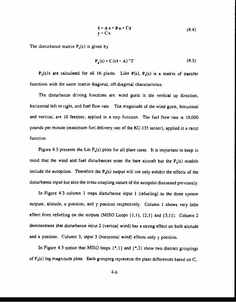
i = Ax +B u + d (4.4)
y = Cx
The disturbance matrix Pd(S) is given by
Pd(s) = C(sI - A)-'1- (4.5)
Pd(S)'s are calculated for all 16 plants. Like P(s), Pd(s) is a matrix of transfer
functions with the same matrix diagonal, off-diagonal characteristics.
The disturbance driving functions are: wind gusts in the vertical up direction,
horizontal left to right, and fuel flow rate. The magnitude of the wind gusts, horizontal
and vertical, are 10 feet/sec, applied in a step function. The fuel flow rate is 10,000
pounds per minute (maximum fuel delivery rate of the KC-135 tanker), applied in a ramp
function.
Figure 4.3 presents the Lm Pd(S) plots for all plant cases. It is important to keep in
mind that the wind and fuel disturbances enter the bare aircraft but the Pd(s) models
include the autopilots. Therefore the Pd(S) output will not only exhibit the effects of the
disturbance input but also the cross-coupling nature of the autopilot discussed previously.
In Figure 4.3 column 1 maps disturbance input 1 (refueling) to the three system
outputs, altitude, x position, and y position respectively. Column 1 shows very little
effect from refueling on the outputs (MISO Loops {1,l}, {2,1] and (3,1)). Column 2
demonstrates that disturbance input 2 (vertical wind) has a strong effect on both altitude
and x position. Column 3, input 3 (horizontal wind) effects only y position.
In Figure 4.3 notice that MISO loops {*,1 ) and {*,2} show two distinct groupings
of Pd(S) log magnitude plots. Each grouping represents the plant differences based on CL.
4-6

)ISooi. I I.' - M%.Ob oop 1.2 I MISO lo 11.31
-40 *0.
100 -
• 25 ' -I
013
- i .10 1
-1001 -IND
3D -4 -20.11
f q ah ) f : f . J, 3 .,
" 0 01 1 10 00. 01 0 1 I 10 100 1I i 1 10. 100
-MSi Ip -,1 - IS.O loP 12 0W MISOoloop 1.-I 1
-40 40 10
-00. 20
j 0
-11140
-100 1 -00.0-160-00
_____f I mdh, ) I f fI~1~. rd&-.)
. 0 -- -. - - . 0- 10 10001 .1 10 JO0.1 1 0 _100.
So, , 13.11 , -- - -SO . L13.21 ,, Io , I 11.
.1i0 4-0 P0g.l-100 -10 4 O
-230. -140 20
-260 .10.
.ppndi D.wMD
.300 -220!
Th snledttd ie nth MS los fFigure 4.3 Pd ts) log Magnitude pPlots
the disturbance rejection specification. Log magnitude of P ' above this line indicates
4-7

that the output due to disturbance exceeds the disturbance rejection specification for the
frequencies that lie above the line. P,(s) MISO loops {,3}, {2,3), {3,1}, and {3,2) are
below the disturbance rejection line, thus, further justifying the break down of this 3x3
system into 2 systems, 2x2 and lxl.
4.4 Sunmary
In this chapter, LTI models and Bode plots for P(s) and Pd(s) are generated. The
calculation of the Q(s) matrix is discussed as well as the significance of channel 3 being
uncoupled from channels I and 2. The next chapter describes the AFCS QFT design.
4-8
V. QFT AFCS Design
5.1 Introduction
This chapter details the QFT AFCS design. First the disturbance rejection
specification is identified. Next, design of the loop transmissions for all three channels
is described. This chapter, nor this thesis, is a detailed step-by-step guide for the QFT
design process. The reader is assumed to have at least a basic understanding of the QFT
method.
5.2 Disturbance Rejection Specification
The primary goal in designing the AFCS systerri is to regulate the position of th-
aircraft receiving fuel relative to the tanker. As discussed in Section 2.4, any dcviation
from the nominal set position is considered a disturbance. Hence a disturbance rejection
specification is determined based on modeled disturbance inputs and the basic QFT design
pretense of unit impulse inputs.
Since the most severe disturbance is due to wind, see Appendix D, the disturbance
specification is "tuned" to the wind input of 10 ft/sec. Section 3.4 indicates a maximum
deviation from the nominal set position of 2 feet in any direction will confine the
receiving aircraft to a volume that will permit continued fuel delivery. Therefore the
following disturbance specification is derived. Given an impulse input of magnitude 10
feet/sec, the system response will deviate no more than 2 ft. Additionally, the system
5-1

will attenuate to half the maximum deviation in less than 1 second. Equation (5.1)
identifies the transfer function for the disturbance rejection specification, and Figure 5.1
shows the disturbance rejection model response to an 10 ft/sec impulse input.
Disturbance rejection model r 400s (5.1)(s + 1)(s + 5)3
1.2 .
.8
.3 -
-. 3
0 .5 1 1.5 2 2.5 3 3.5 4 4.5 5
Tirrt (sec)
Figure 5.1 Disturbance Rejection Model Response to 10 ft/sec Impulse
In Figure 4.1 the Lm of the disturbance rejection specification is superimposed over
the Lm P(s) M1SO loop plots. Notice that MISO loops 12,1), 13,1}, (3,2), (1.3), and
2,3) are below the disturbance specification before compensation is applied.
5-2

5.3 Loop Shaping
The order of loop shaping is determined by the amount of cross coupling each MISO
loop exerts on each other. As discussed in Section 4.2, channel 2 couples strongly into
channel 1. Therefore, channel 2 is designed first, the improved method is applied to
utilize the known g, to recalculate the disturbance bounds for channel 1. Channel 1 is
then designed. Channel 3 is designed last since it is completely decouple and considered
a lxi SISO system.
The bandpass of the plants are relatively low, a bev.'tfit of the autopilot, in shaping
the loops the cverall system bandpass is designed to remain approximately equal to the
plant bandpass. This requirement may require tradeoffs on meeting certain higher
frequency bounds.
5.3.1 Channel 2 Loop Design
For channel 2 plant case 2 is chosen to be the nominal loop. Plant 2 is chosen
because through initial design attempts it proved to be the most difficult to shape around
the stability contour. A successful shaping of plant case 2 guarantees stability for all
plant cases. Templates, stability and disturbance boundaiies are calculated, see Appendix
E. Composite bounds are formed in the MIMO QFT CAD Package. The channel 2
plants are 360 degrees out of phase between the plants derived from aircraft with C,, =
0.2 and CL = 0.6. This is evident from the 360 degree wide templates and the stretching
of the bounds over 360 degrees. The phase difference did not present a problem as the
MIMO CAD Package was able to accommodate this scenario. Compensator g2 poles and
5-3

zeros are added to shape the loop. Channel 2 is relatively easy to shape and proved to
have the lowest order compensator, g,. shown in Appendix F.
Shown in Figure 5.2 the channel 2 loop easily satisfies all QFT loop shaping
requirements for composite bound and stability contours, guaranteeing a stable design
satisfying the disturbance rejection specification. Figure 5.3 shows the Nichols plot for
all 16 plants. From this figure the 360 degree phase difference in the plant is evident.
Though there is a phase difference, each plant correctly goes around the stability contour
indicating a stable design for all plant cases. The following compensator is designed for
channel 2.
92 (s+O.25)(s-,O.75)(s+ 1.2)(s+ 1.3) (5.2)s (s + 0.98±1 )(s + 1O)(s + 20)(s + 120)
5-4

Open Loop Transmission for Channel 2
.!i . i . / _~-- ,f____
60.1 __ I ___ _______ ___________
I _ _ _ _I ___ ___ __ __ __50
. -_ __- -
__° _ ___ -- j I ___ _____ ___ __
__i-I I__ __ i -I __ -" -~
301[__I I'
.30.' I
20. ' _
I
10
-70. _
.WT _
__90.__ -- ---- _ _ _ _ -.--... _ _ - _ _ _
.9o -w _________-_
'~~4.I_____ L____ ! _____ ____
o. -340. -320. -300. -280. -260. -240. -220. -200. -180. -160. -140. -120. -100.
Figure 5.2 Channel 2 Loop Shaping P. = Plant Case 2
5-5

s-DomL Open Loop Transmissions for Channel 2
F74 -
5
44 -- 4 2
0.. 2040 I 1O197-1h) 18c i 711
-15
5-

5.3.2 Channel 1 Loop Design
After g2 is designed the improved method is applied using the equations derived in
Section 2.4. Utilizing the known structure of g2 a more accurate calculation of the cross-
coupled disturbance from the compensated channel 2 to the uncompensated channel I is
achieved. New disturbance and hence composite bounds are generated, shown in
Appendix E. The new bounds have smaller magrutude, thus, overdesign is reduced.
For the same reason as channel 2, the nominal loop for channel 1 is plant case 2.
A-gain, as in channel 2 the templates show a 360 degree phase difference between the two
plant cases of CL = 0.2 and 0.6. But unlike channel 2 there is a magnitude uncertainty
evident in the channel 1 templates, see Appendix E. The magnitude uncertainty arises due
to the strong coupling from channel 2 into channel 1, and also from the difference in the
effect of wind disturbance between the 2 classes of aircraft plants based on CL. The
plants of CL = 0.6 have a larger wind induced disturbance as shown in Appendix D.
Therefore these plants have not only more external disturbance, but also larger cross
coupling disturbance.
The loop shaping is more difficult for channel 1. The loop tends to curl at certain
frequencies as shown in Figure 5.4. The curling causes a large change in phase with little
or no change in magnitude. This type of behavior makes it difficult to shape a loop that
is stable, satisfies the composite bound criteria, and maintains a low system bandpass.
The loop for channel 1 is shaped with a compromise on the bandpass. A lag-lead
compensator is used to "stretch" the low frequency curl. Additional lag-lead compensators
are tried to further "stretch" the curl but caused the loop to increase in magnitude as the
5-7

frequency increased. A loop shape is finally achieved that satisfies the lower frequency
bounds, stability, and slightly increases the system bandpass. The channel I compensator,
g,, has a higher order than the channel 2 compensator, see Appendix F. This is an
indicator of the difficulties in achieving a loop shape that satisfies design criteria.
The Nichols plot of all 16 plants in Figure 5.5 shows the uncertainty in the low
frequency range of the plants. Though there is large phase and magnitude differences
between the plants the QFT method is able to achieve a design that satisfies stability and
disturbance rejection for all plant cases. The following compensator is designed for
channel 1.
g = (s + 0.3)(s + 0.25± 0.433)(s + 3)(s + 9)(s + 1.14± 3.747)(s + 200) (5.3)
s(s+ 2)(s + 0.32± 3.184)(s +90± 4.02D-6)(s + 135± 65.38)(s+ 1100)
5-8
i I II iI

Open Loop Transnision for Channel I
1l0. i i--i-
90.
70o.- ,,-
OVJ 9
I4..... - i "i
j0. '-I
.20. ______
-30-__ _ _
40v _ _ _
.'80 -6 -240 -220 200. 180 -160 -140 -120 100 . . ---60
Figure 5.4 Channel 1 Loop Shaping P. Plant Case 2
5-9

s-Domain Open Loop Transmissions for Channel 1120.1 I
100. -f
81D..
70.L60.- -- ~
30. -- 4---j
-4Q.I.
-20. t ,I-
.30.
-1000 _
-50[I111 i -- i-'-
-70. J1I ----80.~~-90.K t~ ~x-100~ -2
1111 '
80-1.64.020.
-25-10

5.3.3 Channel 3 Loop Design
Channel 3 exhibits none of the channel I or channel 2 characteristics. The channel
3 templates have relatively small phase and magnitude uncertainty. There is no coupling
from channels I or 2 into channel 3. The external disturbances have similar effects on
channel 3 for all plant cases.
The lack of cross coupling disturbance and relatively certain external disturbance is
evident in Figure 5.6 where the bounds collapse around the stability contour. The channel
3 loop has a tendency to curl up as the frequency increases. The main difficulty is to add
compensation to shape the loop around the bounds and stability contour at +180 degrees
and then add further compensation to keep the loop from penetrating the stability region
at -i80 degrees. To achieve stability the very low frequency bounds are penetrated. This
tradeoff is considered acceptable since channel 3, y position has the largest margin of
disturbance allowed, 7.5 feet, as detailed in Section 3.4.
The Nichols plot of Figure 5.7 shows a very tight grouping of all plant cases. Again,
further evidence of relatively small uncertainty in channel 3. Notice the large change in
phase with no decrease in magnitude. This is deemed acceptable since it occurs below
the zero dB line at frequencies below the cutoff. The following compensator is designed
for channel 3.
9 3 (s + 0.05)(s + 0.1)(s + 0.2)( + 0.6)(s + 1.5± 2.6)(s + 5)(s+ 30) (5.4)
s(s + 2.5D-4)(s + 0.6± 1.91 )(s + 10)(s + 35± 35.707)(s + 37.51 64.95)
5-11

Open Loop Transmission for Channel 3
70 Oki49 4
60 0..... ... ... '.
40.'
30 iItIII I '101
-10.+ wi I K'I20. LI i L [' '
Figur 5.6 Chne 3 opSaigP PatCs1
-60.~~ 12......

s-Domain Open Loop Transmissions for Channel 3
90.. kJ T - T'
I T71
40.1 ' I30.----4 Nilt0.5 Lx,
10.1 F--- r2'4
10.~
40. -~ -'ii-..- -
-90.- -4i ----- I
*1 34Q3230262412g8glQ14O1210&80604o-20 0 20 40 608100120140160180200224(260.
Figure 5.7 Channel 3 Nichols Plot all Plant Cases
5-13

5.4 Closed Loop Lm Plots
The overall equivalent MISO system closed loop Lm plots are shown in Figure 5.8.
From these plots you can easily see that disturbance rejection specification is met for all
MISO loops except fc as noted in the low frequency portion of the MISO loop {3,3}.
MISO loop (1. 1) MISO loop (1.21 MISO loop (1,31
-201 -20. -20.,-40.' 1 OL -40..60. -60. :I 7 -60.-80 , -80. -80.
-100. 100 -100.-120.' -120.' -120.-14& -140 i -140.f r160)l " 160 -160. '180 f (rad/sec) , 18o f (rad/se.8o- ,
1Wi . 10 1 . - 2% .i ,. o0. 100. . 6-
MISO loop (2.11 MISO loop (2.2) MISO loop (2.310-0 0
-20. .20 -20.-40' -40 40.-60.' 6 -60..-80 -80.1 -80.
-1o -100.1 ' -100.-120.' -120 . -120.-140.! -140. 1 -1 4 0 .1-160. -160.1 -160.l
f (rad/secr) -180.1 f(rad/se -180.2% 1 . 10. 100. 2(A )]0. .21% .1 . 10.
0 ISO loop 13.1} MSO l1oo2 13.2) MISO loo 3-2_' . I .20 l (3.122)4p 8.-20.1 . -20. "" -20.
40. 40 -4 0 .-60i 1 .60.1 -a0.-80 ' -80. i r- -80.
-100] -100. -100.-120'- -120. -120..140, -140 -140..160. -160 i -160.
- 0 - (ra sc)180 I f (rad/sec)' f (rad/sec)j2 _2I fa/e:) 10.1 -280'% 2° 1! 1. 10 100 .0% ?. .. --. . -- o
Figure 5.8 MISO Equivalent System Lm Plots
5-14

The closed loop MISO plots of Figure 5.8 are an excellent indicator of success m meeting
the design specification.
5.5 Sumniarv
In this chapter the AFCS is designed. Each loop shaping is detailed, covering the
particular difficulties in shaping the loops for each channel. Also the inherent nature of
QFTs ability in handling large plant uncertainties is discussed. Finally the Lm of closed
loop MISO system is shown, indicating a successful design given the tradeoffs made. The
next chapter discusses the linear and nonlinear simulations.
5-15

VI. Air-to-Air Refueling Simulations
6.1 Introduction
In this chapter the compensators designed in the previous chapter are installed in the
AFCS and simulations are run to analyze their performance. Linear simulations are run
for all plant cases in MATRIX x. Nonlinear simulations are for two plant cases, one for
each CL = 0.2 and 0.6, are performed in EASY5x.
6.2 Linear Simulations
Linear simulation are performed in MATRIXx with the modeled external disturbances
forcing the system to deflect from the set point. The simulations are executed in the
presence of all external disturbances simultaneously.
The results of the linear separation for channel I (Z separation) demonstrate excellent
results with very little perturbation from the set point. Figure 6.1 presents the channel 1
response. The plots demonstrate two distinct responses corresponding to aircraft CL. The
aircraft with CL = 0.2 show a maximum perturbation of approximately 0.0025 feet. Also
the response dampens faster for the aircraft modeled with CL = 0.2. The aircraft with CL
= 0.6 deflected to a maximum value of approximately 0.008 feet with slower dampening.
The channel 2 (X separation) linear simulation demonstrates similar characteristics
for response based on CL. Again, excellent rejection of external di, urbance is achieved
as shown in Figure 6.2. CL = 0.2 aircraft have a maximum defloction of approximately
6-1

0.025 feet, while CL = 0.6 aircraft deflect approximately 0.425 teet from the set point.
Recall that the aircraft with CL = 0.6 have a larger uncompensated perturbation due to
external wind disturbance.
Channel 3 (Y separation) has the largest p.rturbation from the set point in the linear
simulation, see Figure 6.3. The maximum perturbation in channel 3 is approximately 1.9
feet. Though considerably larger than channels 1 and 2, the channel 3 perturbation
remains within the design specification.
6.3 Nonlinear Simulations
The nonlinear simulation are performed in EASY5x. EASY5x has a Dryden wind
gust model preprogrammed in the CAD package. The Dryden wind gust model is used
in the nonlinear simulations verses the disturbance model developed in Chapter III. Two
nonlinear simulations are run. One representing an aircraft with CL = 0.2 and the second
for CL = 0.6. The nonlinear simulations require considerable time to setup and perform,
therefore, time limitation prevented performing a norlinear simulating for each plant case.
The nonlinear simulations demonstrate the spme excellent results that are achieved
in the linear simulation. The nonlinear results are consistent with the linear results, very
small perturbations for channels 1 and 2 with a larger deflection in channel 3, shown in
Figure 6.4 and Figure 6.6. As in the linear simulations, the nonlinear simulations are
within the design specifications.
Also presented in the nonlinear simulation plots, Figure 6.5 and Figure 6.7, are the
control surface and thrust response of the autopilot. The aileron, rudder, and elevator
responses are well within the physical capability of these devices. On the other hand the
6-2

thrust requirements are probably beyond engine response capability. The engine response
is most likely due to the autopilot design. The autopilot is a "text book" design and is not
very sophisticated. A QFT design using the actual C- 135B autopilot can probably achieve
similar results without extreme engine response requirements.
o.4 Summary
The compensators designed in Chapter V are integrated into the air-to-air refueling
AFCS. Linear and nonlinear simulations are performed with excellent results. The
system response is within design specification. The QFT design process worked
extremely well in designing the AFCS in the presence of external output disturbance. The
next chapter contains the conclusion and recommendations for this thesis.
6-3

.01
.0 0 .. .... . - -. - --
.004 .. ....
.002.7
I Ll0
'-.004 -
-.008
.0120 1 2 3 4 5 8 7 a 9 10
Time (sec)
Figure 6.1 Linear Simulation -Z Separation Deflection all Plant Cases
6-4

.45
4J I
Time (sec)
Figure 6.2 Linear Simulation - X Position Deflection all Plant Cases
6-5

2
1.8~
1.4
1.2 --
.21
-6-

.06
.04 -
N 0
S-.0204
-. 06.06
.04
.02
S0
-. 02
- .061.2
.9
.3
S 0
-. 60 2 4 8 a 10 12 14 16
Time (sec)
Figure 6.4 Nonlinear Simulation - X, Y, Z Position Defection, Plant 1 CL =0.2
6-7
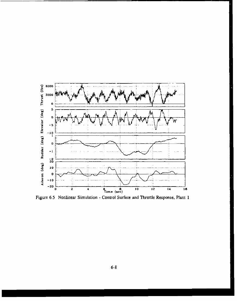
8000
00
- 2
20
10........
00 -z
S-10
-20
028a 0 114 1
a--

.2
-. 4
-. .4.........
.2
0
0
1._6
0 2 4 a 10 12 14 16Time (sec)
Figure 6.6 Nonlinear Simulation - X, Y, Z Position Deflection, Plant 2 CL = 0.6
6-9

6000
3000
I-. 3000 _ _ _ _ _ _ _ _ _
i 1010
0
2
I [0
-220
0!
-40 _______ _
0 2 4 8 a 10 12 14 16Time (Sec)
Figure 6.7 Nonlinear Simulation - Control Surface and Throttle Response, Plant 2
6-10

VII. Conclusions and Recommendation
7.1 Discussion
The purpose of this thesis is to develop an AFCS to regulate the position of a
cargo/transport aircraft relative to the tanker during air-to-air refueling using QFT. To do
this aircraft models are developed that envelop the structured uncertainty of the fuel
receiving aircraft. The uncertainties are based on dynamic changes in the aircraft due to
taking on fuel and the varying CL. Once the aircraft models are developed, an autopilot
is designed to control altitude, speed, and heading The autopilot crsres a stable
minimum-phase plant with a low frequency cutoff. Disturbance models are developed to
identify the effects of wind and refueling disturbances on the plant. The disturbances
enter the system at the plant output, therefore, the QFT equations are redeveloped to
include the effect of external output disturbance. Since the MISO equivalent is not
diagonal dominant, the improved method QFT equations are rederived to include the
external disturbance. The MIMO QFT CAD package, developed by Mr Richard Sating
is used to design the compensators for the control system. After the loops are shaped the
QFT designed compensator are included in the control system where linear and nonlinear
simulations are performed. The linear simulation uses the disturbance model to generate
the external output disturbance. The Dryden wind gust model is used in the nonlinear
simulations.
7-1

7.2 Conclusions
MIMO QFT CAD Package An outstanding QFT design tool. The CAD package
greatly enhanced the design process. Though problems were initially encountered,
they were quickly solved and the package proved to be very robust and easy to use.
QFT External Output Disturbance Equations The successful design of compensators
based on these equations and the subsequent simulations validate that the equations
are correct. These equation are now part of the MIMO QFT CAD Package and
should prove to be valuable in future QFT design work.
Air-to-Air Refueling AFCS The excellent results from the linear and nonlinear
simulations demonstrate the very real possibility of being able to implement this
system on Air Force aircraft.
7.3 Recommendations
The successful simulations the QFT designed air-to-air refueling prove the technology
exists to develop this AFCS. Further research should be accomplished using more
modern aircraft with actual inservice autopilot. Upon successful conclusion of this
research , the Air Force should give serious consideration to implementing this system.
7-2

Appendix A. C-135 Nondimensional Stability Derivatives
This appendix contains the nondimesioard stability derivatives used to generate the
C-135B baie aircraft model.
A.] Nondirnensional Stability Dcrivative Definiiions
A.]. Lonitudinal
C1, - Aircraft drag co .... ient
C - Aircraft lift coefficient
C, - Lift curve slope
C1, - "Change" in lift due to a change ir elevator deflection
C,: - "Change" in pitching moment due to a change in alpha
C,,, "Change" in pitching moment due to a change in alpha rate
Cm,,q "Change" in pitching moment due to a change in pitch rate
Cm,,: "Change" in pitching moment due to a change in elevator deflection
,4.1.2 Lonitudinal
Cyl "Change" in side force due to a change in beta
C)1 - "Change" in side force due to a change in roll rate
C), - "Change" in side force due to a change in yaw rate
C ,F 'Change" i, side force due to a change in rudder deflection
C,?.- "Change" in side force due to a change in aileron deflection
C~,- "Change" in rolling morncnt due to a change in bcta
A-I
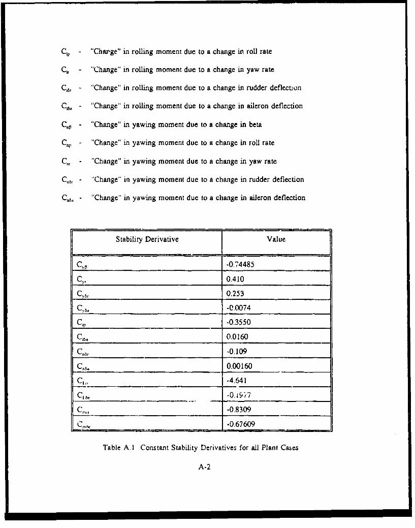
CI- "Charge" in rolling moment due to a change in roll rate
C, - "Change" in rolling moment due to a change in yaw rate
C16- "Change" in rolling moment due to a change in rudder deflection
Ca "Change" in roiling moment due to a change in aileron deflection
CO "Change" in yawing moment due to a change in beta
Cp "Change" in yawing moment due to a change in roll rate
C r "Change" in yawing moment due to a change in yaw rate
C,,e, -"Change" in yawing moment due to a change in rudder deflection
C.- "Change" in yawing moment due to a change in aileron deflection
Stability Derivative Value
CO -0.74485
C ,r 0.410
C),r 0.253
C 69 -0.0074
CiP -0.3550
C16, 0.0160
cr, -0.109
C,6 0.00160
C1,- -4.641
C, Ix -0.19,7
C , ....- 0.8309
Co ,m -0.67609
Table A. 1 Constant Stability Derivatives for all Plant Cases
A-2

Stability Derivative [[Value
CL 0.2 0.6
CYP -0.237 -0.196
Cm -0.17762 -0.22059
C1, 0.108 0.192
CIb, 0.03724 0.0258
C,, 0.15183 0.16043
C,,. 0.0 -0.006
C,, -0.183 -0.187
C R -0.014 -0.03
Table A.2 Stability Derivatives that Change with CL
Gross Center of Cmt C,,q Ixx ( I,Weight Gravity (x 106) (x 106) (X 106)
(xl0 lbs) (% MAC)
1 160.166 28.8 -6.10 -14.25 2.0 2.70 4.575
2 207.316 28.0 -6.13 -14.5 2.725 2.70 5.375
3 210.189 30.1 -6.03 -14.275 3.15 2.75 5.85
4 245.500 22.9 -6.35 -15.025 3.175 2.855 6.0
5 253.500 26.0 -6.22 -14.725 3.1875 3.0 6.1
6 263.500 23.8 -6.30 -14.925 3.2 3.05 6.19
7 275.500 24.1 -6.30 -14.915 3.525 3.10 6.5
8 277.500 248 -6.27 -14.835 3.55 3.105 6.51
Table A.3 Stability Derivatives that Change with Weight and Center of GravityA-3

Appendix B. Plant Transfer Functions
This appendix presents transfer functions for all plants developed with EASY5 and
MATRIX.
B.] Plant Case 1 - CL = 0.2 Gross Weight = 160,666 pounds
2.05D-3(z* 0.286±4.346)(s- 17.22(S 43.763±73.228)(J+ 159.108)($. 499.104)(j- 2.068±6.221)(s- 0.067)s- 0.754±1.208)(j* 5.394)(s* 1.169)(s- 70.040±71.419ys+ 119.979)
2.42D 13(s - 17.223)(s - 43.763 ± 73.228)( - 159.108)s - 249.323 ± 433.b97)( - 499.104)
s(s -6.27D -4 2.3.64D - 4)(s *0.001)(s' - 1)(, -.50)(s 444.55 7.28D 4)(1 - 6.35D -4 ± 3.64D - 4)
q. 0
-12.732.(s 0.269±4.346)
(s- 0.023±0.013)(s* 0.977± 1.718)(s 10.031)
49.866 (s 0.289 14.346)
s(s- 0.099)(s 0.289± 4.336)(s* 501.611)
q- 0
q32 0
2.296 (s - 0.037 1 1.739)(s - 0.2)(1 - 0.289)( 5.620 ± 6.110)q'" s(s - V 146±0.072)(, 0.285)(s* 1.1 15)((5- 5.430±5.951)(s-7.136))
B.2 Plan( Case 2 - CL = 0.6 Gross Weight = 160,666 pounds
q - 2.7D -3 4- 0.471t4.346)(s' 17.223y,'- 43.123 iT72.056)4,' 16e.6q(s- 369.868)" s - U.268t 19.366)(' 0.22 ±0.920)(s w 0.067)4 - 1.362)(1 - 14.24), 70.799±71.556)1 • 119.674)
B-i

.1 83D -16(s o.471,4.364)(s 1 29e?(s 43.123 ,7 • (s116.599)(. _49279,433.31)(. +369.1a
j (i -0004) - 0.286 4.340)(s -1)(s0
q13- 0
-12.853(s - 0.477 *4.364)q ( - 0.025*0.040)(s - 0.759 m1.818)j - 10.029)
37.163(S - 0.477 t 4.364)j.(s 0.101)(s- .473t4.341)(s- 376.574)
q23 0
4 31* 0
q32 0
q 2215 (s -0.095 1 1.76S)(S +0.2)(1 -0.496)(s -5.615 t 6391).i4s -U. 138)(4 -0.156)(a - 0.34)(.Y- 1.44)(i -1.957)(1 +5.392 ± 5.795)(s 7.019)
B.3 Plant Case 3 - C, = 0.2 Gross Weight = 207,316 pounds
2.04D -3 (s + 0.208± 3.697)(s 17.275)( s 43.356172.537)(a 162.16 1)(aj 413.414)(s- 2.119±6.292)(s* 0.062)(s 0.704±0.391)Xjs 5.40)(s* 10.176)(j- 70.032±71.430)(s 119.994)
q, 1..508D - 16(s- 17.275)(s 43.356 ± 72.537) 162.161)(a*249277t433.702)(s 413.414sOs -0-002,1 *()j - 50)
q ,- 0
-13.62 1 f's 0.209± 3698)(s - 0.029)(s- 0.019)4 - 0.89t,1.701)(o - 10.030)
41.405(, - 0M09M± 3 )j(s* 0.099)(s' 0.211 t 3.90)(s 418.121)
q2I- 0
B-2
I Em i

qjI , 0
2. 113 (s - 0.060 it 1.483)s - 0.2)(1 5.445 .4-68)q3 = (*0.154:t 0069)( - 1.275 t 0.444)(- *527014.318)(s -7.739)
B.4 Plant Case 4 - CL - 0.6 Gross Weight = 207,316 pounds
S 2.60D-3(s- 0.3803.719)s. 17.350)(0. 42.80±71.411)(s- 168.723)(s 322.491)(j- 0.748±19.295)Xs 0.062)(j 0.076t.684)(0 1.263)(s- 14.283)(i 70.628 ±71.744)(s 119.960'
-549.466(1 0.381 1 3.718)(s - 17.351)(1 +42.805 W 71.41 1)(s 16& 724)(1 249.302 * 433.469)(s - 322.4906)q'" s(s - 1.695D - 9) ( - 0.007)(1 - .207 3.690)(1 - 1)(s + 50)( s19 D - 9)
q -0
-12.738(s + 0.384±3.718)q2 - 0.027 t0.032)( - 0.61111.B15)(s. 10.029)
32.740s. 0.384 *3.718)(s 0.100.)(.- 0.383±3.702)or+ 332.784)
q123 *0
q 0
qj2- 0
2.052(s -0.133± 1J30)(0.0.2)(s+0.518)(a. 5.422.4,002)s(5 +0.126 )(s -0(.176)s -0. 3 4 7 ) 1.348 ± 0.625)( -5.228t4.106)(1 -7.636)
B-3

B.5 Plant Case 5 - CL = 0.2 Gross Weight = 210,189 pounds
2.01D-3 0.2X7,3.6"74)(s+ 17.280)(s 41321*72.474)(s 162.466)(. 407.121)Lr- 2.122316.252)(s 0.062)(s 0.702a0.875)Cs* 5.368)(1r- 10.172)(1 70.031±71.429)(v. 119.994)
8.854D 4(s. 17.280)(s *43.321 ±71.474)0(162.466)0 •249.276±433.686A) 407.121)"(s-4.185D-6±7.249D6)(s-O.002)(s- 1)(.S0)(s..371D*9)
qI3 0
-13.365(1 0.209 * 3.674)(.7- 0.030)(s- 0.018)(s 0.87 4 t I689)(s* 10.030)
40.792( * 0.209± 3.674)i(s 0.099)(s 0.210,3.67)(js 412.067)
q2 - 0
431- 0
q32 - 0
* 1.833L-0.079 ±1I12)s-0.2)(o 5.4,0±3.S22)s(j *0.155 0.069) 1.143±0.571)(s .5.210,3.523yj 7.961)
B-6 Plant Case 6 - CL = 0.6 Gross Weight = 210,189 pounds
0.298(s- 0.3843.695)(s- 0.062)(1 * 0.090±0.679)±j 1.260)( 114.471)
- 6.175D -3 (s - 0.34 1 3.695)ju (s -0.007)(1 -0.207 ± 3.667)(1 1)
q ,- 0
-13.475(- 0.384±3.694)(jr- 0.027 4 0.032)(S 0.589;± 1.799XV 10.028)
B-4

32.229(s* 0.384±3.695)5(3 0.100)(s 0L392±3.678)(s+ 327.733)
12- 0
q3,", 0
qu.- 0
3 1.776(s -0.150 * 1.558)(s -0.2)( +0.524)(s + 5.374 ± 4.070)"(s - 0.125)s -0.177)(s -0.349)(s - 1.213 ± 0.720)(s +5.169± 3.262)4 - 7.878)
B.7 Plant Case 7 - CL = 0.2 Gross Weight = 245,500 pounds
5.252(s- 0.170s3.361)(s+ 0.058)(s 0.677±0.7101(s' 8.867)(s- 119.936)
5.244D - 3(s -0.170 ± 3.36.1)sO' - 0.003) s0.169± 3.35 1 )(j - 1)
3* 0
-13.193(s- 0.170±3.361)(s - 0.037)(s - 0.013)(s 0.840± 1.639)(1. 10.029)
35.848(s 0.170±3.361)s(sv- 0.098)O.- 0.1723.354)(S- 363.322)
q- 0
q*j 0
q*. 0
1.965(s-0.071 ± 1.346)(s-0.2)(s*0.266)(,5.381 ± 3.799)qj .s4 0.158)(s *0.067)f - 0.273)(s- 1.099 ±0.591)(s -5.207 ± 3,486Xs * 6.049)
B-5

B8 Plant Case 8 - CL = 0.6, Gross Weight = 245,500 pounds
0.294(s - 0.341t3.332)(s 0.058)(1 0.106t0.606)(1 1.213)(1 - 128.756)
5.285D -3(s 40.341 ± 3.382)$(j -0.008)(s* 0.169 3.352)(1 * 1)
413 0
q21 - 13.296(1 - 0.34113.382)(s - 0.027 ± 0.027)(1- 0.517± 1.575)(s - 10.027)
=n 28.999(s + 0.341 ±3.382)s( s 0.100)(s - 0.339 ± 3.367)(s-+ 295.845)
q, . 0
q31* 0
q32- 0
q-j 1.924(s -0.141 ± 1.407)(s -0.2)(I 40.530)( *5.352 14.014)s(s - 0.123)(j - 0184)(s + 0.349)(1 + 1. 163 ± 0.735)(s - 5.165 3.233)(s. 7.957)
B.9 Plant Case 9 - CL = 0.2, Gross Weight = 253,500 pounds
0.058)s 4.94(s 0.168±3.313)
(s + 0.058)(s - 0.672 ± 0.679)(s - 8.896)(s 11 7665)
5.07OD - 3(j -0.166 t 3.313)s(s - 0.003)(s -0.167 ± 3.303)(1 - 1)
qL3 - 0
-12.519(3 s 0.16813.313)
(s - 0.038)( - 0.012)(s 0.793 ±1.603)(s, 10.027)
B-6

34.607 Q 0.168 *3.313)2 (3 0.098)(s- 0.170±3.306)(s 351.087)
q3,- 0
4.973(s -0.070 11.32 1)(s -0.2)s 0.2641)(s 5.379± 3.780)- a(s -0. 159± 0.066)(5 - 0.272)(s. 1073 ± O.6)(s - 5.205 3.467)(s &094)
B.1O Plant Case 10 - CL = 0.6, Gross Weight = 253,500 pounds
- 0.279(s. 0.339 t 3.334)(i- 0.05 8)(s- 0.111 1,0-591)(, - 12,03)(j - 126.-502)
5.118D-3(s -0.339±3.334)q1 2 $(S-0.008)(,s0.167±3.304)( +1)
q13- 0
S -12.617(s 0.339±3.334)(s- 0.028 ±0.026)(s - 0.476 * 1.713)(s + 10.026)
27.906(s * 0.339 ± 3.334)s(s- 0.l00)(s- 0.337±3.A19)(s- 285.044)
q23 0
q 3 1 - 0
q-2 0
1.913(1 -0.155 1 1.39 3)(j - 0.2)(1 0.31)Xi - 5.349t3,992)s(s 0.12.2)(1-185)(10.349)(S- 1.135 t-0.7W4(S .5.164t 3220)(s-LOM7)
B-7

B.11 Plant Case 11 - CL = 0.2, Gross Weight = 263,500 pounds
4.921 (S - 0. 160 ±3.243)q(S -, 0.057)(S* 0.666*642)(g. S.904)(+ 120,454)
4.U5D - 3(1 0. 10 ± 3.243)s (s - 0.003)(s -. 159 1 3.232)(s -1)
q1 - 0
-12.361 (. 0.160 ±3.243)(s - 0.039)(1 - 0.01 1)(s + 0.7 2 ± 1.585)(s 10.027)
q2 ' 33.432(s - 0.160 t 3.243)
j(s- 0.098)(s* .162±3.236)(s+ 339.502)
-0
q3, s0
q33 0
- 1.975 (s - 0.067 ± 1.290)(s -01)(s 0.261)(s - 5.376 ± 3.762)ij" s(, -0.160± .066)(s 0.270)V - 1.051 0.616)s +5.204 * 3.450)(1 s.&132)
B.12 Plant Case 12 - CL = 0.6, Gross Weight = 263,500 pounds
0.276(s - 0.330 3.64)(s.+ 0.057)(s- 0.117 ±0.574)(s- 1.193)(j- 129283)
4.924D-3(s.0.3303.264):(s-0.008)(4+0.158±3.234)(s51)
q13. 0
- 12458(j- 0.330±3.264)
(- 0.028±0.025)(3w 0.458±1.696)(j 10.025)
B-8

27.074(3- 0.330±32 )
.(s+ (1100)(s. 0328,3.250)(s. 276.840)
Q2j 0
qj3I 0
q3 0
1.916(s -0.155 ± 1.356)(1 - 0.2)(3 - 0.532)(1 -5.346 ± 3.971)0 (. - 0.122)(s - 0. 87)(. - 0.349)(s -. 1111 0.754)s - 5.162± 3.206)(s. &05O)
B.13 Plant Case 13 - CL = 0.2, Gross Weight = 275,500 pounds
4.870(1- 0.15313.164)q (j 0.056)(s- 0.659±0.601)(,- 8,909)(s 124.191)
4.672D - 3(j 0.153 *3.1 .q (3 -0.003)(.q + 0.152 ± 3.153)(s - 1)
qu- 0
-12.232(j* 0.1533.164)
(S- 0.040)(s- 0.010)(s- 0.763 1.569)(1- 10.027)
32.169(S 0.153 ±3.243).(s 0.098)(s.+ 0.1553.157)(s 327.051)
q23" 0
q3* 0
q,2 0
q 1.875 (1 - 0.072 1.266)( -0.2)1 - 0.258)(1 .5.347± 3.248)$(,-0.162 :±.065)(s0.269)(s 0.990 ±0.647)(s 5.169± 3.I . Ui &240)
B-9
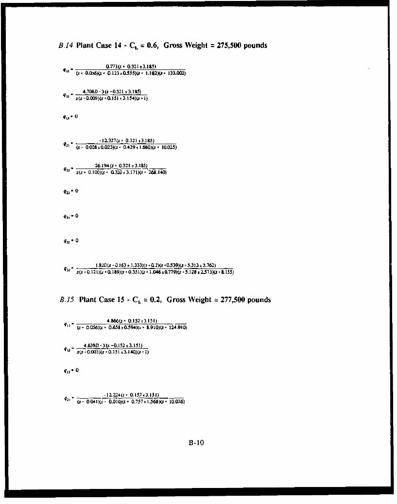
B.14 Plant Case 14 - CL = 0.6, Gross Weight = 275,500 pounds
0.273(s - 0.321±3.185)(s4 O.06)(s 0.123±0.5)s- 1.182)(s- 133.002)
4.708D- 3(s -0.321 ±3.185)Ut (s -0.009)(s 0. 151 t 3 .154)( 1 - )
qu = 0
-, - ~ -12.327(s * 0.321 13.185)(i - 0.028 i 0.0f23)(s - 0.429 11 O)(s + 10.025)
26.194(s - 0.321 13.185)s(s- 0.1O0)(s- 0.320± 3.171)(s- 268.140)
q23- 0
q31 - 0
-s: 0
1.820(s -0.163 ± 1.333)(* 0.2)(s '0.539)(s *5.313 i 3.762)433. s(s -0.12i)(1 .189)(s -0.351)( 1.048 ±O.779)(s -5.128 ± 2.573)(S 8.155)
B.15 Plant Case 15 - CL = 0.2, Gross Weight = 277,500 pounds
4.866(s- 0.152t3.151)(t+ 0.056)(s* 0.658,0.594)(.v* 8.910)(s* 124.910)
4.639D - 3(s .0.152±3.151)j(s- 0.003)(s -0.151 13.140)(1 - 1)
q13 ' 0)
-12.224(S4 0.152±3.151)(a- 0.041)(- 0.010)(s, 0.757±1.568)(s 10.026)
B-10

S 31.972(s - 0.152 13.151)s(js 0.098)(t. -(154:k 3.144)(1+ 325.094)
q- 0
qj - 0
*n 0
1.879(s -O.G1 t 1.259)(S -0.2)(s 0.257)(s -5.344 3.210)s(s -0.162 0.065)(s * 0.269)(1 - 0.988 ±0.648)(1 -5.167 2.26)(s - &242)
B.16 Plant Case 16 - CL = 0.6, Gross Weight = 277,500 pounds
0.273(s - 0.321 ± 3.172)(sI 0.056)(s - 0.124 1.0-552)(s- 1.180)(1 - 133.736)
4.675D- 3(s 0.321 ±3.172)s($ -0.009.1(s-0.151 :t 3. 142)(s. - 1)
q13 ' 0
- 12.319(s - 0.32113.172)2 ,(S - 0.(P,, ± 0.02 Vs - 0.4211 ± 168)( - 10.02,5)
26.060(s- 0.321±3.172)s(s- 0.099)(s, 0.319-3.158)(s 266.819)
q=23 0
q31t 0
q32 0
1.824(s -0.163 t 1.327)(1 - 02)(s + 0.539)(s - 5.310 13.420)s(s - 0. 121)(s O. 189)(s - 0.351)(; - 1.046 ± J.7)(s 5.126 ± 2.520)(s 8-157)
B-II

Appendix C. C-135B and Autopilot Input Response
This appendix contains the time response plots for the C-135B and autopilot.
C-1

0
,-2
.'40
S20
0
-.0005
0
-0001
0 10 20 30 40 s0 80Time (vec)
Figure C.1 Mach Hold Response to I ftisec Step Input - CL = 0.2
C-2

60
C20L_ _ _ _ _ _ _ _
0 F.
-0036-
010- 20 30 40 so 60Time (Sec)
Figure C. 2 Mach Hold Response to I ft/sec Step Input - CL = 0.6
C-3

0
.001
0_
- 0 0 1 -.... -
- 0020~
M'~0002[
0U
- 5.0AE -07 ----
- 1.OOE-08______________________
0 10 20 30 40 50 80Time (aec)
Figure C.3 Altitude Hold Response to 1 foot Step input - CL 0.2
C-4
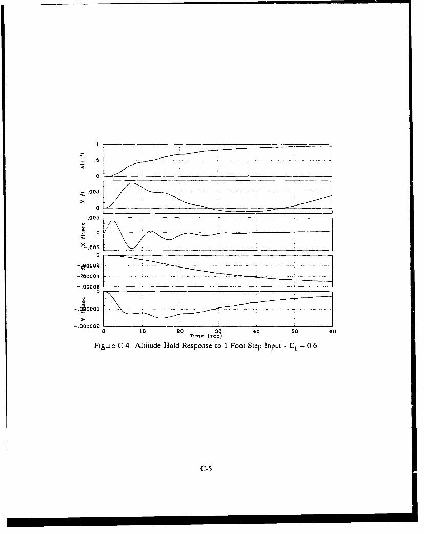
-.003 10
.005
- 0k-
0
-epO002
-. 000080
-. 000 IL
-. 00000 10 20 30 40 s0 60
Time (isec)
Figure CA4 Altitude Hold Response to 1 Foot Step Input - CL = 0.6
C-5

0
.0001
001-
100_ __ __
0
2
0
0
tJC-6

-20002F
0-ln
-. VO005
-. 0001I
200
*. 2
. 0-
~; .30~
0 10 20 30 40 so soTime (sec)
Figure C.6 Rudder Control Response to 1 deg Step Input - CL 0.6
C-7

.00004
.0O002
0
0
U0
- :00 05-
8500
Z: 300'
0
c10
0.

.00006
410003 - --
0
-. 000c -
L? 0
A 0005
'v 0001600
300
0
0 10 20______0___ 40______ 0_____ 0_
Time (see)
Figure C.8 Aileron Control Response to 1 deg Step Input - CL 0.6
C-9

Appendix D. C-135B and Autopilot Disturbance Response
This appendix contains the time response plots for the C-135B and autopilot in the
presence of external disturbance.
1-I

0
-1.8 2
10
X 4
-. 00005
- .0002-
-. 000250 3 6 9 12 1~ 18 21 Z4 27 30
Time (6e0)
Figure D.1I X, Y, Z Response to Longitudinal Wind Disturbance - CL =0.2
D-2

0
-10
*-20
-40180
150-
120 -
go60
'J0
0
-. 001[
>--.003 -
-. 004--
- .0050 3 8 9 12 1 5 1 18 21 24 27 30
Time (sec)
Figure D.2 X, Y, Z Response to Longitudinal Wind Disturbance - CL = 0.6
D-3

.00002 ......
0001 -
-.000002-
- .000004
A 0 0 ... .. ....
- .000008
-. 00001
-. 000012100
40
0 3 6 a 12 1~ 18 21 24 2? 30Time (81e11
Figure D.3 X, Y, Z Response to Lateral Wind Disturbance - CL = 0.2
D-4

.00004
.00J003
A.00002 -
-.000012
80
-. 0
0
-. 0 0061 L 8 2 2 7 3Time (mec)
-.Figr . ,YZRsos t aea in itrace-C .
-. 000 12 .. .......
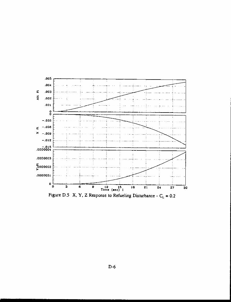
.005
Z .002
0
0
003
.0000
.0000004
.0000003 --- 'i-
0 Time 1 (uc 5 18 21 24 27 30
Figure D.5 X, Y, Z Response to Refueling Disturbance - CL =0.2
D-6

.08
.08* ----
S .04 ---.-...-- ~ -
.02 .- - -- -- --
00
-. 2 - ---
.000008
.000006 -
U00004 - -
.000002 - ---
0 3 6 9 12 t5 is 21 24 27 30Time (ec)1
Figure D.6 X, Y, Z Response to Refueling Disturbance - CL =0.6
D-7

Appendix E. Templates and Boundary Plots
This appendix contains the template plots. It also presents the stability and
disturbance boundaries used to form the composite bounds.
E-I

db Templates -Channel I -Nominal Plan: Case 2
400
w=0.01 W=O 1 w=0.5 w=0.6 w0.7
300
w--0.8 w=0.9 w=l. w3. w=3.6
200 -4;.5
100 W=7.5 w=10. w=20. w=30, w=50.
_ i i i I i I., . , I . . . ,i i I i i | i
500 1000 1500 2000 2500degrees
Figure E. 1 Channel 1 Templates
E-2

0 _'____ F
10 4 -.7. "
4~6 4 4x
"° ! I ',o
Figure E.2 Chanel I Stability Bounds
E-3

60/"-
50 "-40
I 'I "' . ]_I: - '
3 ,. i I I I __ __I . -T 1 1 ,
I 1"---
-1-0- -... ,-- _ __/ -._' - ---4
-. -340 -320 -300 -280 -260 -240 -220 -200 -180 -160 -140 -120 -100 -80 -60 -40 -20
Figure E.3 Channel 1 Disturbance Bounds
E-4

db Templates - Channel 2 - Nominal Plant Case 2
50
,!0O.01 w!=O. I W!Zi5 w 3.6 w=0.7
40
,!7w=. w1 w--3. w-3.6
30
w=4. w-4.25 w45 W:;4.75 v=
20
4=. =10. w=20. w--30. w=50.
10
So0 1000 1500 2000degreem
Figure E.4 Channel 2 Templates
E-5

II
I PS.. i. ul.- _ _ _-
I4-
:0- 1- :° - Nt\l' . .!.. J .--,S ' i I ii
I , ',
"2 60 -340 -320 -300 -2 ' )-260 -2 0 220 200 -180 -160 -140 -120 -100 -80 -60 -40 -20 0
Figure E.5 Channel 2 Stability Bounds
E-6
I I I I I II

80[ i -[ 11 - t,., 1,l ] , I' 1-f I
8 0 - I I
901 T
o I I
I tI J
Figure E.6 Channel 2 Disturbance Bounds
E-7
s o L -, ]

Templates - Channel 3 -Nominal Plant Case 2
50~ N0Yw=0.01 w=O.I w-0.5 w0.6 w--0.7
40
w=0.8 wffO.9 wfil. =3. w--3.6
30
w=. w-4.25 w=4.5 W4.75 w-5.
20
w=7.5 w=10. w=20. 30
10
* I , I * ' | I , I " I
50 100 150 200 degrees
Figure E.7 Channel 3 Templates
E-8

20L
! ! I I
10 -- _.- Ir , _
I o I
Vi
I , I
-340 -320 -300 -280 -260 -240 -220 -200 -180 -160 -140 -120 -100 -80 -60 -40 -20 0
Figure E.8 Channel 3 Stability Bounds
E-9

100 F i i
9Cr 1 _____ i I 7801 " I I
60.: I I ,I I
T 1 , ' " 4 1 _ .' ! - I II-
, II I
40 i II I I '
20 1 * I ___
20-I
10: , ti l
IIT___-- I ___ Izz~ 1 I ____--
-2.tU -340 -320 .300 -280 -260 -240 -220 -200 -180 -160 -140 -120 -100 -80 -60 -40 -20 0
Figure E.9 Channel 3 Disturbance Bounds
E-IO

Appendix F. QFT Comipensators
This appendix contains the comnpensators designed in Chapter V.
F.1 Channel 1 compensator, g.
(s + 0.3)(s +0.25± 0.433)(s + 3)(s +9)(s + 1.14± 3.747)(s + 200)(-)s (s +2)(s +0.32 ± 3.184)(s +9 0± 4.02D -6)(s + 135±t 65.38)(s + 1100)
F.2 Channel 2 compensator, g,
(s + 0.25)(s + 0.75)(s + 1.2)(s +. 1.3) (F-2)s (s +0.98± 1)(s + 10)(s + 20)(s + 120)
F.3 Channel 3 compensator g.,
(s + 0.05)(s + 0.1 )(s + 0.2)(s + 0.6)(s ' 1.5± 2.6)(s + 5)(s + 3n) (F-3)s (s + 2.5D-4)(s +0.6± 1.91 )(s + 10)(s +. 35± 35.707)(s + 37.5 ± 64.95)
F- I
Bibliography
1. The Boeing Company. Summary of the Stability, Control and Flying QualitiesInformation for All the -135 Series Airplanes. Technical Report D3-9090 REV LTRA, Wichita KS, October 1073.
2. D'Azzo, John J. and Constantine H. Houpis. Linear Control System Analysis andDesign, Conventional and Modern (Third Edition). McGraw-Hill, 1988.
3. Ho,,pis, Constantine H. Quantitative Feedback Theory (QFT)--Technique forDesir);ing Multivariable Control Systems. Technical Report AFWAL-TR-86-3107,Wrignt-Patterson AFB, OH: Flight Dynamics Laboratory, January 1987.
4. Sating, Richard R. QFT CAD Package. MS thesis, Air Force Institute ofTechnology, Wright-Patterson AFB, OH, March 1992.
5. Boeing Computer Services, Seattle, WA 98124-0346. EASYSx - User's Guide,January 1992
6. Blakelock H. John. Automatic Contro! of Aircraft and Missiles (Second Edition).Wiley-Interscience, 1991.
7. MATRIX x CAD/CAE Program, Integrated Systems Inc., South Matick, MA, 01760.
8. Pachter, Meir, "Personal Conversation, Correspondence and Class Notes." Professorof Electrical Engineering, Air Force Institute of Technology, Wright-Patterson AFB,OH, May 1992 through June 1993.
9. Houpis, Constantine H., "Personal Conversation, Correspondence and Class Notes."Professor of Electrical Engineering, Air Force Institute of Technology, Wright-Patterson AFB, OH, May 1990 through June 1993.
10. Rosrm, Jan. Airplane Flight Dynamics and Automatic Flight Controls, Part I.Roskam Aviation and Engineering Corp., 1982.
11. Military Specification - Definition of Atmospheric Disturbance Model Form. MI.-STD 1797(USAF) APPENDIX A. 31 March 1987.
BIB-I

Vita
Captain Dennis Trosen was born on 10 August 1962 in Detroit, Michigan. He
graduated from Waterford Township High School, Waterford Township Michigan in 1980.
He attended Michigan Technological University and received his Bachelor of Science in
Electrical Engineering in May of 1984. He received his commission from Officer
Training School in August 1984. He was first assigned to the 6585th Test Group at
Holloman AFB New Mexico were he was a guidance system component test engineer and
then program manager for the Advanced Guidance Technology test program. In 1990 he
was reassigned to the Foreign Aerospace Science and Technology Center at Wright-
Patterson AFB Ohio, where he performed technology analysis of foreign C3 systems. In
June 1992, he entered the School of Engineeiing Air Force Institute of Technology
studying for a Masters of Science degree in Electrical Engineering. Upon graduation from
AFIT he will be assigned to Wright Laboratory at Wright-Patterson AFB, Ohio.
Permanent address: 124 ExmoorWaterford, Michigan 48054
VITA-I

REPOT DCUMNTATON AGEForm ApprovedREPOT DCUMETATON PGE MB No 0704-0188
ovoIl reD'- r_,a'e' , ~ ietC fl'lhf -t'ie lo, &,efa.e !.v n Dvtop -easeoe,inc uding the tte for re~iew.ng instructions hearcn-r,' . %ling datasovr~cengae"'; a -4".'ta -. '9 ie dat3nee-de-d ad<(On'Detng d fei' I the ~e~ n ,,naton Sena~o (Oments regarding In-$ burden etifnate Or an, Othe, aspect of 1hVrflient~ O'mlltc. in( n S.,9eitir fer reducing In sDuraen tc wasington MeaaoiarletC' ot . 'ecto'ale for imo'va,o.i one-azins and RL-pcq. 12tS jetlersor.
i., '24r.intcn -2 22202-430?. ano ': te OE4.ceol M#nagenrrn aNd D.,dge! tape-o-i, Red.e-,,Pr,ect(0?04-0188) v-shringto.. DC 20S03
1. AGENCY USE ONLY (Leave blank) 2. REfOBRT DA E .ReR ltffN DATES COVEREDI Jue 193R asrTT Stiesis
4. TITLE AND SUBTITLE S. FUNDING NUMBERSDEVELOPMENT OF AN AIR-TO-AIR REFUELINGAUTOMATIC FLIGHT CONTROL SYSTEM USINGQUANTITATIVE FEEDBACK THEORY
6. AUrHOR(S)Dennis W. Trosen
7. PERFORMING ORGANIZATION NAME(S) AND ADORESS(ES) 8. PERFORMING ORGANIZATIONAir Force Institute of Technology, WPAFB OH 45433-6583 REPORT NUMBER
AFIT/GE/ENG/933-03
9. SPONSORING; MONITORING AGENCY NAME(S) AND AODRESS(ES) 10. SPONSORING!. MONITORINGWright Laboratory AGENCY REPORT NUMBER
FIGSWPAFB 011 45433-6583
11. SUPPLEMENTARY NOTES
112a. DISTRIBUTION AVAILABILITY STATEMENT 12b. DISTRIBUTION CODE
Distributirnn Unlimited
13. ABSTRACT (Maximum 200 words)
Abstract
Quantitative Feedback Tlheory and the improved method Quantitative Feedback Theory are enhancedto include the rejection of disturbance at the system output. The enhanced Quantitative Feedback Theoryand improved method Quantitative Feedback Theory processes are applied to the design of an automaticflight control system to regulate position of the C-135B fuel receiving aircraft relative to the tanker duringair-to-air refueling. A simple feedback control system is developed that will achieve stable position regulation.State-space aircraft modelb are generated. An "inner loop" autopilot is designed to reduce the plant cutofffrequency and provide the system inputs for the Quantitative Feedback Theory compensators. Disturbancemodels representing disturbance due to wind gusts and refueling are developed. The flight control system isdesigned using the enhanced Quantitato.,c Feedhack Theory equations. Linear simulations are performed onMATRIX, and nonlinear simulations are run on EASY5x. The results of the simulations show excel-lent results.The simulation results indicate that air-to-air automatic flight control system wec technically achievable, andthat implementation in USAF aircraft is possible.
14. SUBJECT TERMS 15. NUMBER OF PAGESQFT1, flight control, air-to-air refueling, 125disturhance rejection, regulation control 16. PRICE CODE
17. SECURITY CLASSIFICATION 18. SECURITY CLASSIFICATION 19. SECURITY CLASSIFICATION 20. LIMITATION OF ABSTRACTO E PORT OF THIS PAGE OF ABSTRACT
NtI.c ASSIFIED UNCLASSIFIED UNCLASSIFIED UL
NSN 7540-01-280 5500 Stan~dard Formn 298 (Rev 2-89)PM r10 Dy AN', Std 139-IB19

GENERAL INSTRUCTIONS FOR COMPLETING SF 298
The Report Documentation Page (RDP) is used in announcing and cataloging reports. It is importantthat this informaton be consistent with the rest of the report, particularly the cover and title pageInstructions for filling in each block of the form follow It is important to stay within the lines to meetoptical scanning requirements
Block 1 Agency Use Only (Leave blank) Block 12a. Distribution/Availability Statement.Denotes public availability or limitations. Cite any
Block 2. Reo Date. Full publication date availability to the public. Enter additionalinc~udchn o j' mc°n and yea', if available (e.g. 1 limitations or special markings in all capitals (e.gJan 88). Must (,e a, least the yea, NOFORN, REL, ITAR).
Block 3. Type of Report and Dates Covered. DOD See DoDD 5230.24. "DistributonState vihcthe- report is riterm, final, etc If S e e on Technicalapp!icable, enter inclusive report dates (e.g. 10 Documents. T*Jun 87 - 30 Jun 88) DOE See authorities.
Block4. Title and Sub!'tle A title istaken from NASA - See Handbook NHB 2200 2.the part of tre repo-' tria: prcviies the most NTIS Leave blank.
meanngf ,!and comp'ete infui maton Whenareport is prepared .n mo'e than one volu'me, Block 12b. Distribution Code.repeat the priray title, add volume number, andinclude subt-tle for tne speo:fic volume Onclass'fied d~ocumernts er-te- the tt~e c',ass fication DD-Laebakclafin rt e s hDOE - Enter DOE distribution categoriesin parentheses from the Standard Distribution for
Block S. Fund:nc N.,mbes To include contract Unclassified Scientific and Technicaland grant ncrmbe's. may Include p'ogram Reports.element , tk NASA- Leave blank.eeetnumbens,. oto, eoct number(s), tasknurrber(s). and wC un:t number(s) Use the NTIS - Leave blank.
fo:'o,'.ing laLE s.
C Cont'act PR Project Block 13. Abstract Include a brief (MaximumG Cranq: TA Task 200 words) factual summary of the mostPE - Proc,&am WU Work Urit significant information contained in the report.
Eier enz Accession No
Block 6. A ci. Name(s) of person(s) Block 14. Subiect Terms Keywords or phrasesresponsb'e for wvti*g the report, performing identifying major subjects in the report.the research, or credted w th the content of thereport If ed.tor or comp!.er, this should followthe name(s) Block 15. Number of Pages. Enter the total
number of pages.Block 7. Perfor:ro Organization Name(s) andAddre~s~es, Selfepanatoy Block 16. Price Code Enter appropriate price
Block 8. Performio Organization Report code (NTIS only).Number Enter the unique alDhanumeric reportnumber(s) ass.gned by the organizationperforming the report Blocks 17.- 19. Security Classifications. Self-
explanatory. Enter U.S. Security Classification inBlock 9. Sonsorirnqlrvloltornq Agency Name(s) accordance with U.S. Security Regulations (i.e,and Address(e5) Self-exp'anatory UNCLASSIFIED) If form contains classified
information, stamp classification on the top andBlock 10. Spor-.or".cio-tornq Agency bottom of the page.Repo - t Numbe- (If known)
Block 11. Supplementary Notes Enter Block 20. Limitation of Abstract This block mustinformatior no' included elsewhere such as be completed to assign a limitation to thePrepared incoopera.ionw th. "Trans of , To be abstract Enter either UL (unlimited) or SAR (samepublished in Vvhen a repo-t is revised, include as report). An entry in this block is necessary ifa statement whether the new report supersedes the abstract is to be limited If blank, the abstractor supplements the older report is assumed to be unlimited
Stancard Foirm 298 Ba( (Rev 2-89)I I I,,
Recommended