DESIGN OPTIMIZATION OF FOLDING SOLAR POWERED AUTONOMOUS
UNDERWATER VEHICLES USING ORIGAMI STRUCTURE
A Thesis
by
DOE YOUNG HUR
Submitted to the Office of Graduate and Professional Studies of
Texas A&M University
in partial fulfillment of the requirements for the degree of
MASTER OF SCIENCE
Chair of Committee, Richard J. Malak
Committee Members, Darren J. Hartl
Douglas Allaire
Head of Department, Andreas A. Polycarpou
August 2017
Major Subject: Mechanical Engineering
Copyright 2017 Doe Young Hur
ii
ABSTRACT
Origami, as an application for morphing structure engineering, which has been
studied for a long time, has recently made remarkable progress in terms of technology.
The most distinctive feature of this technology is the presence of two types, flat mode
and folded mode. The origami algorithm enables the conversion of these two modes
based on the mathematical formulations. Completion of this algorithm now means that
origami is part of the design process and can be applied to applications.
This thesis demonstrates a design process for origami-inspired morphing
structures that transform between a flat configuration and a folded convex shape. There
are many obstacles in the development of the design process. In particular, consideration
should be given to the surface difference of the flat configuration and the folded convex
mode. In this thesis, I introduce the design process which takes into consideration the
origami structure design deeply.
To demonstrate this process, I have selected an application which is emerging
and interesting, that is, unmanned vehicles. Especially, the design of Autonomous
Underwater Vehicles (AUVs) is a difficult challenge since it requires the consideration
of various aspects such as mission range, controllability, energy source, and carrying
capacity. The Predictive Parameterized Pareto Genetic Algorithm (P3GA) is selected as
the optimization method to determine a parameterized Pareto frontier of design options
with desired characteristics for a variety of missions for the AUV.

iii
ACKNOWLEDGEMENTS
I would like to thank my committee chair, Dr. Richard Malak and committee
member Dr. Darren Hartl for full support and guidance in minute detail. Committee
member Dr. Douglas Allaire, for the support throughout the course of this research.

iv
CONTRIBUTORS AND FUNDING SOURCES
This work is supported by the National Science Foundation and the Air Force
Office of Scientific Research under grant EFRI-1240483. Any opinions, findings,
conclusions or recommendations are those of the authors and do not necessarily reflect
the views of the U.S. Air Force. The authors would like to acknowledge Dr. Douglas
Allaire for providing the main idea for the study presented in this work. Computational
fluid analysis was performed using a research license granted by ANSYS. The
optimization studies were conducted using Matlab, courtesy of Mathworks.

v
NOMENCLATURE
H1 Height of AUV (m)
L1 Length of front region (m)
L2 Length of rear region (m)
KR1, KR2 Input variables of shape function
d Characteristic length of the mesh faces (m)
w Characteristic length of the tucked regions in the origami design (m)
C Length of AUV for shape function (m)
Z Height of AUV for shape function (m)
CD Drag coefficient
CM Moment coefficient
Area Available area for solar panel (m2)
Volume Available volume inside the body (m3)
𝜂𝑒 Efficiency of electrical speed controller
𝜂𝑃 Efficiency of propeller
𝜂𝑀 Efficiency of motor
Ec Collected energy
Drag Drag force

vi
TABLE OF CONTENTS
ABSTRACT .......................................................................................................................ii
ACKNOWLEDGEMENTS ............................................................................................. iii
CONTRIBUTORS AND FUNDING SOURCES ............................................................. iv
NOMENCLATURE ........................................................................................................... v
TABLE OF CONTENTS .................................................................................................. vi
LIST OF FIGURES ........................................................................................................ viii
LIST OF TABLES ............................................................................................................. x
1. INTRODUCTION .......................................................................................................... 1
2. ENGINEERING DESIGN PROBLEMS ....................................................................... 6
2.1. Origami Structure……………………………………………………………6
2.2. Solar Powered Autonomous Underwater Vehicle…………………………...8
2.3. Overall Design Process…………………………………………………..…10
3. ANALYSIS AND OPTIMIZATION TOOLS……………...………………………15
3.1. Three-dimensional Modeling based on Shape Function………………….15
3.2. Origami Modeling………………………………………………………..18
3.3. Computational Fluid Analysis……………………………………………...21
3.4. Available Solar Area Calculation…………………………………………..23
3.5. Available Inner Volume Calculation………………………………………24
3.6. Mission Range Calculation……………………………………………...….27
3.7. Parametric Optimization using P3GA……………………………………...28
vii
4. RESULTS………………………………………………………………………31
4.1. Design of Experiment……………………………………………………....31
4.2. Validation of Models……………………………………………………….34
4.3. Physical Characteristics………………………..…………………………...39
4.4. Pareto Front………………………………….………………………….….47
5. CONCLUSIONS .......................................................................................................... 51
REFERENCES ................................................................................................................. 52
viii
LIST OF FIGURES
Figure 1. Trade-off between Folded Convex and Flat Configuration ................................ 3
Figure 2. Planar Configuration of Designed Origami Sheet that Maximizes Projected
Area of Solar Panels (Top), Goal Configuration Obtained after Folding
(Bottom) .............................................................................................................. 7
Figure 3. Concept Design of Solar Powered AUV, Adapted from [36] ............................ 9
Figure 4. Overall Design Process ..................................................................................... 12
Figure 5. Flowchart of Analysis Approach ...................................................................... 12
Figure 6. Side View and Top View of The AUV Shape and Brief Description of
Dimension Parameters ...................................................................................... 16
Figure 7. AUV Model with H1=1.27 m, L1=1.05 m, L2=3.3 m (LEFT) and H1=0.72
m, L1=0.85 m, L2=3.74 m (Right) ................................................................... 17
Figure 8. An illustration of an existing advanced front mesh generation concept in
two dimensions. The dotted line indicates the current front. The new
triangle is created one at a time by joining the two leading edges to the
newly created point or existing lead ................................................................. 19
Figure 9. Three-Dimensional Model Before Meshing (Top) and After Meshing
(Bottom) ............................................................................................................ 20
Figure 10. Example Of Triangular Solar Panel, Adapted from [52] ................................ 23
Figure 11. Edge-tucking molecule is represented in terms of two parameters: w and θ,
Adapted from [53] ............................................................................................ 24
Figure 12. (a) Vertex-tucking molecule surrounded by polygons and edge-tucking
molecules. (b) Vertex-tucking molecule on the boundary, Adapted from
[53] .................................................................................................................... 25
Figure 13. Comparison of Same Model With Different w Value. Same model with
w=0.2 (Top, Available Inner Volume = 2.497 m3) and w=0.6 (Bottom,
Available Inner Volume = 1.165 m3) ............................................................... 27
Figure 14. Flow chart of the P3GA, Adapted from [15] .................................................. 29
Figure 15. An illustration of predicted dominance, Adapted from [60] .......................... 30
Figure 16. Examples of Latin Hypercube Designs, Adapted from [74] .......................... 32

ix
Figure 17. Distribution of Experimental Points (First Generation), Design of
Experiment (TOP), Optimization (BOTTOM) ................................................. 33
Figure 18. Experimental Points (25th Generation), H1 vs CD ........................................ 33
Figure 19. Base Model – 1/10 Scale Typhoon Type Submarine ..................................... 34
Figure 20. Manuevering Case Validation Result ............................................................. 35
Figure 21. Two Types of Tail Wings for Validation. A-Type (Top) And B-Type
(Bottom) ............................................................................................................ 38
Figure 22. Results of Sensitivity Analysis. H1 vs CD (Top) and d vs CD (Bottom) ....... 39
Figure 23. Projected Scatter Plot of All Populations: H1 vs. CD (Top) and d Vs. CD
(Bottom) ............................................................................................................ 41
Figure 24. Projected Scatter Plot of All Populations: H1 vs. Drag Force ........................ 42
Figure 25. Projected Scatter Plot of All Populations w vs. Area ..................................... 42
Figure 26. Projected Scatter Plot of All Populations d vs. Area ...................................... 43
Figure 27. Results of H1 vs. CM grom Sensitivity Analysis (Top) and Projected
Scatter Plot (Bottom) ........................................................................................ 43
Figure 28. Projected Scatter Plot of all Populations H1 vs. Inner Volume (Top) and
H1 vs Range (Bottom) ...................................................................................... 45
Figure 29. Projected Scatter Plot for Range vs Inner Volume of all Populations (TOP)
and Non-dominated Populations (BOTTOM) .................................................. 46
Figure 30. Three-Dimensional Scatter Plot of all Populations for Design of
Experiment ........................................................................................................ 47
Figure 31. Three-Dimensional Pareto Frontiers for Design of Experiment ..................... 48
Figure 32. Three Dimensional Pareto Frontiers via Interpolated Mesh for
Optimization ..................................................................................................... 49
Figure 33. Three Dimensional Scatter Plot of each Unknown Parameter (H1) for
Optimization ..................................................................................................... 49

x
LIST OF TABLES
Table 1. Drag Coefficient of a Sphere relative to Reynolds number [75] ....................... 36
Table 2. Validation Results for Origami Piece Size ......................................................... 36

1
1. INTRODUCTION
Origami allows for the transformation of initially 2-dimensional sheets to 3-
dimensional shapes through folding. Origami engineering is currently applied to an
industrial field such as satellites [1]. Although origami-inspired design promise in some
situations, it is not currently a widely-used technique in the design of engineered
structures and systems. There are two main reasons for this. First, the origami has not
been applied to precision machine industries. Second, there is still lack of the technology
to properly control the origami-inspired structures for industrial applications.
To properly utilize origami technology, it is necessary to develop an appropriate
design process based on an understanding of origami. Unlike the analysis of general
rigid structures, the characteristics of origami as a morphing structure must be carefully
considered to derive its merits. There are a number of additional things to consider such
as total surface area change due difference between the flat configuration and folded
convex, and dividing the smooth surface into flat pieces. Therefore, this thesis introduces
a design process that can take advantage of the original advantage of origami.
In this thesis, I have applied origami-inspired structures to Solar Powered
Autonomous Underwater Vehicle (SAUV) for demonstration. Design of rigid origami,
where the planar facets of the sheet are rigid, is an active area of study [2, 3, 4, 5, 6, 7].
Contributions in this area have enabled novel methodologies for the design of
deployable structures and morphing architectural forms [2, 8, 9, 10, 11, 12].

2
The biggest advantage of the designed origami structure is that it is able to
transform both the three-dimensional shape and the flat surface repeatedly. In this thesis,
I have applied the origami-inspired design to the AUV field.
AUVs have become an application that is widely used in military, oceanographic,
and environmental study. Recent AUV development efforts have focused on range and
endurance for long-term operation. This enables long-term data collection [13, 14].
Four key characteristics are desired for AUVs: hydrodynamic efficiency, mobility,
volume capacity and energy capacity. Among them, energy capacity is the most
important. The AUV is able to conduct measurements at remote locations of the ocean
[15]. A crucial limiting factor for such vehicles is the limited distance that the AUV can
travel with its available energy. This is due to the lack of an inexpensive and effective
energy source. Aside from nuclear sources of energy, a potential solution to this
challenge is to harvest energy from the environment. An accessible source of energy is
solar radiation [16].
In another aspect, some recent works have also considered the problem of finding
the optimum hull form for AUVs to minimize drag. These include the works of Lutz and
Wagner [17], Bertram and Alvarez [18], and Alvarez and coworkers [19]. Small
reductions in hydrodynamic drag can result in substantial savings in thrust requirements
and significant improvement in achieving higher vehicle cruising speeds [20, 21]. As
you can see in the picture below, you can easily compare two extreme cases. Since the
folded SAUV is advantageous in terms of hydrodynamics, the resistance in water is
relatively small and the influence of algae is less. However, even if it floats on the

3
surface of the water, it is not easy to charge because the area exposed to the sun is small.
Conversely, in the case of the flat type, it is possible to secure a large amount of
chargeable area, but it is difficult to protect the internal equipment and has a
hydrodynamic disadvantageous form. Therefore, as shown in Fig.1,origami was applied
to the design of SAUV which can take advantage of these two modes.
Figure 1. Trade-off between Folded Convex and Flat Configuration
There are many obstacles in the development of the design process. In particular,
consideration should be given to the surface difference of the flat configuration and the
folded convex mode. In this thesis, I introduce the design process which takes into
consideration the origami structure design deeply.
More work still needs to be done in terms of optimizing the hull form design to
minimize drag or increase propulsion efficiency [22, 23]. In this thesis, the overall shape
of a novel process, which is explained in sec 2.3 in detail, for solar-powered AUV is
designed.
4
Since new advances in origami design allow for the realization of three-
dimensional goal shapes by folding initially planar sheets, the key step in the design
process of an application is to determine the goal shape. A convenient way to describe a
three-dimensional surface is through combinations of surface functions such as Non-
Uniform Rational B-Splines (NURBS) [12, 13, 14, 24, 25, 26]. Using NURBS, a
complex surface can be mathematized through a finite set of variables. For industrial
applications where performance is dependent on shape, the method is efficient to seek
for an optimum design. Prior to this, however, boundary curves were required to define
the NURBS surface, which used an improved shape function for the vehicle [27], is
parameterized using a low number of variables allowing for efficient optimization.
An origami design method [28, 29, 30, 31] is used to determine a planar sheet
that can be folded towards the AUV shape. As such, origami design allows for the
folding/unfolding of the structure between the AUV shape (to store materials and
navigate underwater) and the planar shape (to maximize the projected area of the AUV
solar panels and to charge the power supplies). The employed origami modeling and
design methods consider smooth folds [28, 29, 30], in contrast to creased folds
conventionally assumed in the literature. Therefore, the folds considered here can be
integrated with active material actuators (since their deformation requires smooth
bending [30]).
Furthermore, I explore how these performance characteristics (hydrodynamic
efficiency, mobility, volume capacity, and energy capacity) are affected by sizing
constraints using parametric optimization [32, 33, 34]. Engineers routinely perform

5
parameter studies to investigate how a system responds under a range of assumptions.
Parametric optimization is an extension that asks how the optimal design changes over
the range of parameters. The result is a description of optimal solutions as a function of
parameter. In this thesis, I use parametric optimization to explore what ranges of
hydrodynamic efficiency, mobility, and energy capacity are achievable as a function of
the AUV size. The results give insight into the capabilities and limitations of the solar-
powered AUV concept. A previously developed algorithm, predictive parametrized
Pareto genetic algorithm (P3GA) [31], is used to solve the search problem.

6
2. ENGINEERING DESIGN PROBLEMS
2.1. Origami Structure
The origami design method previously developed by the authors Peraza
Hernandez and Hartl [28, 31] is utilized. It provides the geometry of a single planar sheet
with a pattern of smooth folds (see Fig. 2) that can morph towards the original input
mesh of the AUV. As shown in the literature [30], there are several critical
characteristics due to the folding of the origami.
The most important feature of origami-inspired design is the folded convex state.
Generally, I can create an origami model that maintains the shape of the initial three-
dimensional input model. The novel origami-based design of the AUV proposed here
allows the folding and unfolding of the structure between the AUV shape optimized for
hydrodynamic efficiency (to navigate underwater and store materials) and the planar
shape (to maximizes the projected area of the AUV solar panels to charge the power
supplies). The employed origami modeling and design methods consider smooth folds
[28, 29, 30] as opposed to creased folds typically assumed in the literature. Therefore,
the folds considered here may have integrated active material actuators (since their
deformation requires smooth bending [30]). The effect of folding on SAUV can be
classified into three types. The volume loss due to the tucked surface of the folded
convex, the change in surface area resulting from exposure of the surface in flat
configuration, and the change in drag due to sharp edge formation on the smooth
surface. The loss of volume is to be treated again at sec 3.5 and surface edge formation
at sec 3.1.

7
Exposed surface area of flat mode is also shown in Fig.1. Unlike the orange
colored region, which always exposed in both modes, the gray colored tucked surface
and the black colored bended surface are not exposed in folded convex. This difference
makes it possible to obtain more exposed areas than conventional single-mode SAUV.
Because of the above features, the design process introduced in this thesis should
consider two modes at once. In this thesis, we set the objective based on the target
performance in each mode and monitor both modes. To improve the performance of
AUV mentioned above, we focused on performance such as Available Area, Available
Inner Volume, and Drag Force.
Figure 2. Planar Configuration of Designed Origami Sheet that Maximizes
Projected Area of Solar Panels (Top), Goal Configuration Obtained after Folding
(Bottom)

8
2.2. Solar Powered Autonomous Underwater Vehicle
It has long been considered that AUVs could provide an effective solution for
surveillance, environmental monitoring and data portal (to sub-sea instruments)
requirements. However, limitations in their battery life have limited the usefulness of
AUVs in such applications. Rechargeable solar batteries have been proposed to enhance
the application of AUV platforms where long-term or ongoing deployment is required
[35]. On the other hands, the importance of oceanographic monitoring has gained
importance as the range of human activities has expanded to the ocean. Current amount
of data gathered from ocean is not enough to fulfill the requirement to understand
chemical, biological and physical characteristics. For example, physical and biological
coupling, biogeochemical processes and cycles both natural and human induced,
fisheries, and ecosystem modeling need more data to analyze more precisely. However,
current data gathering system does not have enough ability to provide enormous size of
the data continuously.
To resolve this issue, a Solar-powered Autonomous Vehicle (SAUV) was
introduced by Blidberg, et al. As shown in Fig.3 [36], the SAUV utilized the solar
energy as an energy source for autonomous data gathering platforms. The model they
introduced has several assumptions. They considered the insolation to be 4.0
kWhr/m2/day (in the southern US), a 10% of conversion efficiency and the PV array of
1.8m2. With these assumptions and the model, they expected 42 km transit at a velocity
of 3.5km/hr. [36].

9
Yet, the design of a SAUVs involves several more competing objectives, it is a
good case-study for the adaptation of origami principles and the performance of multi-
objective design optimization.
Figure 3. Concept Design of Solar Powered AUV, Adapted from [36]
However, this type of AUV is limited by the change of shape due to the solar
panel, which limits the drag reduction and controllability. If the shape of an array with a
solar cell can be modified, it is very helpful to increase efficiency and mobility. To
improve this, I decided to use the origami folding technique. There are two critical
characteristics that I can improve through origami. I can expand exposed surface through
flat configuration mode and reduce drag through the streamlined form folded convex.
10
2.3. Overall Design Process
Numerous coupling methods have been attempted to perform modeling, analysis,
and computation in different fields. One of the biggest obstacles in this process was to
synchronize data in different formats. As different logics or computer languages are
used, various methods have been discussed to convert the interpreted signal and output
data format of each field. For example, C is based on ANSYS Fluent and
supercomputing systems, and Rhinoceros is based on C ++. Origami code and P3GA are
also compiled by Matlab which is based on C ++. To integrate these languages, I
basically used Matlab's batch file processing method, and bundled it into one process
using python scripting, which is commonly used for many programs. In addition, the
output raw data of each analysis was used in the xls format provided by Microsoft Excel
in consideration of the post-processing usability. In addition, three-dimensional model
data was used for the igs, inp, and msh formats.
Overall process is shown in Fig.4. It starts with the selection of initial data points
using Latin Hypercube Design. For more information on Latin Hypercube Design, see
Sec. 4.1. In order to analyze the effectiveness of this process, initial data points were
randomly selected in Optimization # 1, and Latin Hypercube Design was applied to
Optimization # 2. The analysis process is divided into CFD and origami analysis. The
effort in the analysis procedure entails Computational Fluid Dynamics (CFD) analysis.
Using ANSYS Fluent, which is fast and accurate, the drag coefficient (CD) and moment
coefficient (CM) are determined. CD value represents efficiency and CM value represents
maneuverability. A more detailed description of this process is given in sec 3.3.

11
Origami analysis is divided into two categories: Available Area for Solar Cell
calculation and Available Inner Volume calculation. Both procedures use the origami
method introduced in sec 3.2 and the available Inner Volume calculation is calculated
using Rhinoceros as introduced in sec 3.5.
Output data and input data for each process are shown in Fig. 4. Surface data
using NURBS was transferred in igs form. Based on this, two-dimensional surface mesh
data was provided in origami code and Ansys in inp format. Here again, a three-
dimensional mesh was generated in msh format and finally provided to Fluent. Based on
this modeling data, the final output data in the form of xls was generated.
This composition of various engineering analysis tools is currently being
developed and used in many fields, but for automation, it is difficult to integrate and
communicate easily. The methods presented above have their meanings as a means to
overcome the limitations.

12
Figure 4. Overall Design Process
Figure 5. Flowchart of Analysis Approach

13
2.3.1. Design of Experiment
Before the optimization, a demonstration of the optimization was performed for
evaluation of each objectives. The mathematical expression for the demonstration is as
follows:
𝐌𝐢𝐧𝐢𝐦𝐢𝐳𝐞𝐱
𝑭(𝐱,𝑯𝟏) = [𝑪𝑫; −𝑪𝑴; −𝑨𝒓𝒆𝒂]
Where 𝐱 = [𝐿1, 𝐿2, 𝐾𝑅1, 𝐾𝑅2,𝑤, 𝑑]
Unknown Parameter = H1
Subject to 0.7m ≤ 𝐻1 ≤ 1.3m
0.7m ≤ 𝐿1 ≤ 1.3m
2.2m ≤ 𝐿2 ≤ 3.8m
0.5 ≤ 𝐾𝑅1 ≤ 1.1
0.7 ≤ 𝐾𝑅2 ≤ 1.3
0.25m ≤ 𝑑 ≤ 0.75m
0.2 ≤ 𝑤 ≤ 0.4
Variables fall into three categories. First, H1, L1, and L2 are dimensional
variables. These variables specify overall sizes. Second, KR1 and KR2 are shape
variables used in shape functions. The method using these variables is explained in sec
3.1. Third, d and w are variables for origami modeling. d is the characteristic length of
the mesh faces, which is introduced in sec 3.2 and w is the characteristic length of the
tucked regions in the origami design which is introduced in sec 3.5.

14
2.3.2. Optimization for Performance
The performance of the AUV can evaluated by available inner volume (volume)
and mission range (range). The available inner volume decides capacity of the AUV for
experimental devices, battery, etc. Volume is critical for functional expandability.
The overall design process is as follows:
𝐌𝐢𝐧𝐢𝐦𝐢𝐳𝐞𝐱
𝑭(𝐱,𝑯𝟏) = [−𝑹𝒂𝒏𝒈𝒆;−𝑰𝒏𝒏𝒆𝒓 𝑽𝒐𝒍𝒖𝒎𝒆]
Where 𝐱 = [𝐿1, 𝐿2, 𝐾𝑅1, 𝐾𝑅2,𝑤, 𝑑]
Unknown Parameter = H1
Subject to 0.7m ≤ 𝐻1 ≤ 1.3m
0.7m ≤ 𝐿1 ≤ 1.3m
2.2m ≤ 𝐿2 ≤ 3.8m
0.5 ≤ 𝐾𝑅1 ≤ 1.1
0.7 ≤ 𝐾𝑅2 ≤ 1.3
0.25m ≤ 𝑑 ≤ 0.75m
0.2 ≤ 𝑤 ≤ 0.4
15
3. ANALYSIS AND OPTIMIZATION TOOLS
3.1. Three-dimensional Modeling based on Shape Function
A three-dimensional shape of the AUV’s outer surface is generally streamlined
and very complex, and often varies according to its use and operational environment. To
represent the characteristics of the three-dimensional shape configurations in terms of
categories, Calkins and Chan [37] classified automobiles into one-box, two-box, three-
box, etc. In each category, the boxes, which comprise the shape of the automobile, are
divided into section boxes in order to use analytical functions to represent the shape.
This method of decomposition is used in automobile structural design [38]. An
automobile configuration must meet spatial requirements, also referred to as the package
layout [39], including dimensions for the whole body length and width, engine location,
space for the driver, roof and trunk, size of the intake, and front and rear glass. The
entire outer shape of the automobile is determined by a combination of these principal
dimensional variables. Details and attached parts such as bumpers, shoulders, and
internal flows can be represented by dividing the section boxes into smaller parts. The
same process is adapted for this study. Same as a divided automobile, the AUV is
divided into 2 boxes as shown in Fig. 6. The front box is contains the frontal section of
the AUV that is obtained by revolving front curve. The AUV region contained in the
rear box is determined by rear curve and two straight curves.

16
Figure 6. Side View and Top View of The AUV Shape and Brief Description of
Dimension Parameters
H1
L1 L2
L2 L1
H1

17
The curves representing the streamlined outer surface of a vehicle can be
represented using the following function:
F (x
c) = (
𝑥
𝑐)
𝐴1
(1 −𝑥
𝑐)
𝐴2
𝑆 (𝑥
𝑐) + (1 −
𝑥
𝑐)𝑌1 + (
𝑥
𝑐) 𝑌2 (1)
where x and c are the dimension and length of each section box depicted in Fig.6.
The section function S(x/c) provides higher flexibility in the design of the shape
[22]. The modified functions for AUV case considered in this work are given as
follows:
Front Box: 𝑧
𝑐(𝑥
𝑐) = (
𝑥
𝑐)0.5
(1 −𝑥
𝑐) [𝐾𝑅1 ∗ (1 −
𝑥
𝑐) +
1
𝐾𝑅1∗ (
𝑥
𝑐)] + (
𝑥
𝑐)𝑅1 (2)
Rear Box: 𝑧
𝑐(𝑥
𝑐) = (
𝑥
𝑐)0.5
(1 −𝑥
𝑐) [𝐾𝑅2 ∗ (1 −
𝑥
𝑐) +
1
𝐾𝑅2∗ (
𝑥
𝑐)] + (1 −
𝑥
𝑐) 𝑅1 (3)
Where KR1 and KR2 are design variables that decide the overall shape and R1, which is
equal to H1, is radius of the revolving circle located between front box and rear box.
And as both equations contain R1 as common value, they have same value at the point
they meet. The difference between the models according to the variables is shown in the
figure below. The example of H1, L1, and L2 in modeling is shown in Fig.7.
Figure 7. AUV Model with H1=1.27 m, L1=1.05 m, L2=3.3 m (LEFT) and H1=0.72
m, L1=0.85 m, L2=3.74 m (Right)

18
3.2. Origami Modeling
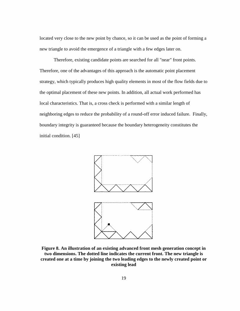
The advancing front method [40,41,42,43,44] is utilized here to determine a
mesh discretization of the AUV surface (see Fig. 8). Advancing Front Techniques begins
with the discretization of geometry boundaries in a two-dimensional corner set. These
edges form the outgoing front face to the field. A specific edge of this face is selected
and a new triangle is formed based on this edge by combining the two ends of the
current edge with the newly created point or the existing point on the face. The current
edge is removed from the front because it is currently hidden by the triangle. Likewise,
as shown in Fig. 8, the remaining two corners of the new triangle are either assigned to
the front or removed from the front, depending on their visibility. Thus, the front can be
removed or removed from the stack where the stack, or priority queue, is configured and
edges are added sequentially. When the stack is empty, that is, when all the faces are
merged together and the domain is completely covered, the process is terminated. One
important feature of these methods is the placement of new points. When creating a new
triangle, the new point is placed first in the determined location to be the optimal size
and shape triangle. The parameter defining this optimal triangle as a function of field
position is obtained by a predetermined field function, which may be interpolated from
the background grid. Triangles created with new points can be rejected because they can
cause crossovers with other front edges. This is determined by calculating the
intersection with the near front edge. Alternatively, the existing point on the front can be
19
located very close to the new point by chance, so it can be used as the point of forming a
new triangle to avoid the emergence of a triangle with a few edges later on.
Therefore, existing candidate points are searched for all "near" front points.
Therefore, one of the advantages of this approach is the automatic point placement
strategy, which typically produces high quality elements in most of the flow fields due to
the optimal placement of these new points. In addition, all actual work performed has
local characteristics. That is, a cross check is performed with a similar length of
neighboring edges to reduce the probability of a round-off error induced failure. Finally,
boundary integrity is guaranteed because the boundary heterogeneity constitutes the
initial condition. [45]
Figure 8. An illustration of an existing advanced front mesh generation concept in
two dimensions. The dotted line indicates the current front. The new triangle is
created one at a time by joining the two leading edges to the newly created point or
existing lead

20
This Advancing Front Meshing technique is applied to determine an origami
sheet design that can be folded towards the AUV shape. A uniform mesh size
distribution is assumed for this problem and therefore only one characteristic length is
required to generate a mesh using the advancing front method. Such a characteristic
length was designated as variable “d” in the design process. A mesh generated through
the advancing front method is shown in Fig. 9.
Figure 9. Three-Dimensional Model Before Meshing (Top) and After Meshing
(Bottom)
21
3.3. Computational Fluid Analysis
A commercial tool ANSYS used for fluid analysis of each case. Boundary
condition was 5m/s for velocity, water, and 0.0001 for residual convergence. The basic
viscous model is k-epsilon with standard near-wall function of ANSYS. I also used
Simple C pressure-velocity coupling technique. Outputs from the analysis are Drag
Coefficient (Cd) and Moment Coefficient (Cm) which are the objectives of optimization
process itself.
In this study, CFD analysis was performed using a standard k-e model. Using a
two-equation turbulence model, you can solve two separate transport equations to
determine turbulence length and time scale. The standard k-ε model of ANSYS Fluent
belongs to this type of model, Launder and Spalding [46] has become a key element in
the computation of practical engineering flows. Robustness, economics, and reasonable
accuracy for a wide range of turbulence illustrate its popularity in industrial flow and
heat transfer simulations. This is a semi-empirical model, and the derivation of model
equations depends on phenomenological considerations and empiricism.
Standard k-ε models [46] is a model based on model transport equations for
turbulent kinetic energy and its dissipation rate. The model transport equation for k-ε is
derived from the exact equation, but the model transport equation for ε is obtained using
physical reasoning and is not nearly identical to the mathematically correct response [47]

22
The governing equations of k-ε is based on three dimensional time dependent
compressible Navier-Stokes equations [48]. The conservation laws of mass, momentum,
and energy and the equation of state for a perfect gas expressed in terms of Reynolds
density-averaged variables and compact tensor notation for j=1,2,3 are
Mass Conservation: ∂ρ
∂t+
𝜕
𝑥𝑗(𝜌𝑢𝑗) = 0
Momentum Conservation: ∂ρui
𝜕𝑡+
𝜕
𝜕𝑥𝑗(𝜌𝑢𝑗𝑢𝑖 + 𝑝𝛿𝑖𝑗 − 𝜏𝑖𝑗) = 0
Energy Conservation: ∂e
∂t+
𝜕
𝜕𝑥𝑗(𝑢𝑗(𝑒 + 𝑝) − 𝑢𝑖𝜏𝑖𝑗 − 𝑞𝑗) = 0
These equations require the definition of the turbulent Reynolds stresses in terms
of known quantities [49]. The stress tensor is modeled as proportional to the mean strain-
rate tensor, and the factor of proportionality is the eddy viscosity for eddy viscosity
models. Reynolds stresses are
𝜏𝑖𝑗 = 2𝜇𝑡 (𝑆𝑖𝑗 −𝑆𝑛𝑛𝛿𝑖𝑗
3) −
2𝜌𝑘𝛿𝑖𝑗
3
where 𝑆𝑖𝑗 =1
2(
𝜕𝑢𝑖
𝜕𝑥𝑗+
𝜕𝑢𝑗
𝜕𝑥𝑖)
and 𝜇𝑡 =𝑐𝜇𝑓𝜇𝜌𝑘2
𝜀
where μt is the eddy viscosity, Sij is the mean-velocity strain-rate tensor, ρ is the fluid
density, k is the turbulent kinetic energy, δij is the Kronecker delta, turbulent dissipation
rate, ε, model coefficient, cμ, is determined by equilibrium analysis at high Reynolds
23
numbers, and the damping function, fμ, is modeled in terms of a turbulence Reynolds
number, Reμ = ρk2/εμ.[50]
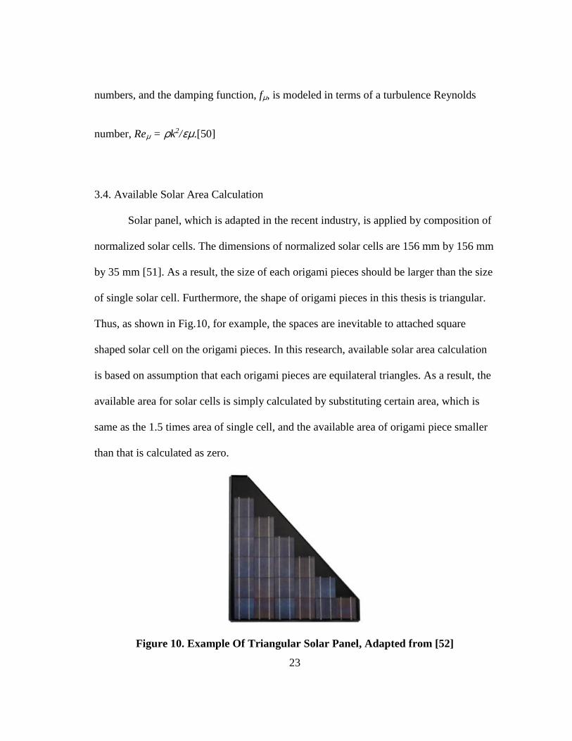
3.4. Available Solar Area Calculation
Solar panel, which is adapted in the recent industry, is applied by composition of
normalized solar cells. The dimensions of normalized solar cells are 156 mm by 156 mm
by 35 mm [51]. As a result, the size of each origami pieces should be larger than the size
of single solar cell. Furthermore, the shape of origami pieces in this thesis is triangular.
Thus, as shown in Fig.10, for example, the spaces are inevitable to attached square
shaped solar cell on the origami pieces. In this research, available solar area calculation
is based on assumption that each origami pieces are equilateral triangles. As a result, the
available area for solar cells is simply calculated by substituting certain area, which is
same as the 1.5 times area of single cell, and the available area of origami piece smaller
than that is calculated as zero.
Figure 10. Example Of Triangular Solar Panel, Adapted from [52]
24
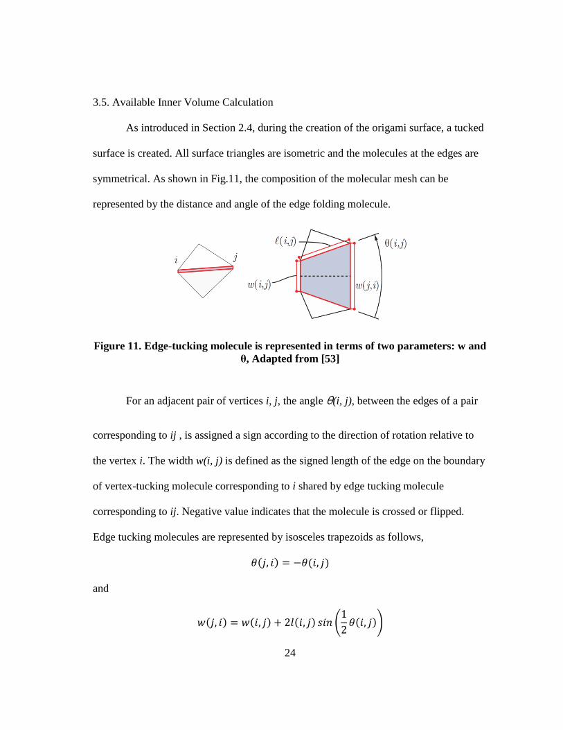
3.5. Available Inner Volume Calculation
As introduced in Section 2.4, during the creation of the origami surface, a tucked
surface is created. All surface triangles are isometric and the molecules at the edges are
symmetrical. As shown in Fig.11, the composition of the molecular mesh can be
represented by the distance and angle of the edge folding molecule.
Figure 11. Edge-tucking molecule is represented in terms of two parameters: w and
θ, Adapted from [53]
For an adjacent pair of vertices i, j, the angle θ(i, j), between the edges of a pair
corresponding to ij , is assigned a sign according to the direction of rotation relative to
the vertex i. The width w(i, j) is defined as the signed length of the edge on the boundary
of vertex-tucking molecule corresponding to i shared by edge tucking molecule
corresponding to ij. Negative value indicates that the molecule is crossed or flipped.
Edge tucking molecules are represented by isosceles trapezoids as follows,
𝜃(𝑗, 𝑖) = −𝜃(𝑖, 𝑗)
and
𝑤(𝑗, 𝑖) = 𝑤(𝑖, 𝑗) + 2𝑙(𝑖, 𝑗) 𝑠𝑖𝑛 (1
2𝜃(𝑖, 𝑗))
25
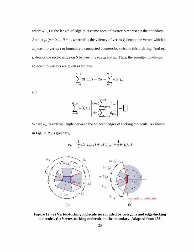
where l(i, j) is the length of edge ij. Assume nominal vertex o represents the boundary.
And let jn (n = 0,…,N − 1, where N is the valency of vertex i) denote the vertex which is
adjacent to vertex i or boundary o connected counterclockwise in this ordering. And α(i,
j) denote the sector angle on S between ijn-1(modN) and ijn. Thus, the equality conditions
adjacent to vertex i are given as follows.
∑ 𝜃(𝑖, 𝑗𝑛) = 2𝜋 − ∑ 𝛼(𝑖, 𝑗𝑛)
𝑁−1
𝑛=0
𝑁−1
𝑛=0
and
∑ 𝑤(𝑖, 𝑗𝑛)
[ cos (∑ 𝜗𝑚)
𝑛
𝑚=1
sin (∑ 𝜗𝑚)𝑛
𝑚=1 ] 𝑁−1
𝑛=0
= [00]
Where 𝜗𝑚 is external angle between the adjacent edges of tucking molecule. As shown
in Fig.12, 𝜗𝑚is given by,
𝜗𝑚 =1
2𝜃(𝑖, 𝑗𝑚−1) + 𝛼(𝑖, 𝑗𝑚) +
1
2𝜃(𝑖, 𝑗𝑚)
Figure 12. (a) Vertex-tucking molecule surrounded by polygons and edge-tucking
molecules. (b) Vertex-tucking molecule on the boundary, Adapted from [53]

26
Due to the tucked surface, as shown in Fig. 13, the difference between the
volume calculated from initial outer surface and the real volume available occurred. To
calculate this volume, many methods were applied. The first method I have tried was
shifting outer surface in orthonormal direction. However, in the process of moving the
surface, a shrink occurs. As a result, a surface break occurred, which results in an open
volume. Since the volume cannot be calculated, I decided not to adopt this approach.
Another method is shifting the outer surface in uniform direction. But it is also not
selected because there is a difference from the actual available Inner Volume.
To calculate this, I need to recreate the available imaginary inner surface, not the
actual outer surface of origami, to calculate the volume. To do this, I have created a
surface based on the center point of each bended surface. To make the surface, I used the
‘mesh from points’ function provided by the Rhinoceros program for surface creation.
The method is based on adjacent points which is an approximation calculated by taking
the square root of the quotient of the area of the bounding box divided by the number of
points [54]. By connecting the points in a triangular shape, meshed surface is created.
Since all the surfaces are created in planar shape, it is easily changed into NURBS
surface which forms a closed volume.

27
Figure 13. Comparison of Same Model With Different w Value. Same model with
w=0.2 (Top, Available Inner Volume = 2.497 m3) and w=0.6 (Bottom, Available
Inner Volume = 1.165 m3)
3.6. Mission Range Calculation
Calculation of mission range is based on several assumptions. Mathematical
expression for range is, 𝑅𝑎𝑛𝑔𝑒 = 𝜂𝑒𝜂𝑃𝜂𝑀𝐸𝑐
𝐷𝑟𝑎𝑔, Where 𝜂𝑒 , 𝜂𝑃 𝑎𝑛𝑑 𝜂𝑀are efficiency of
speed controller, propeller and motor. EC is collected solar energy by solar cells and
Drag is drag force of the AUV. Insolation, the amount of exposure to the sun, is assumed
same as the condition of Hawaii in June, 6000Wh/m2[21,35]. For drag force calculation,
drag coefficient (CD) is calculated through ANSYS.
28
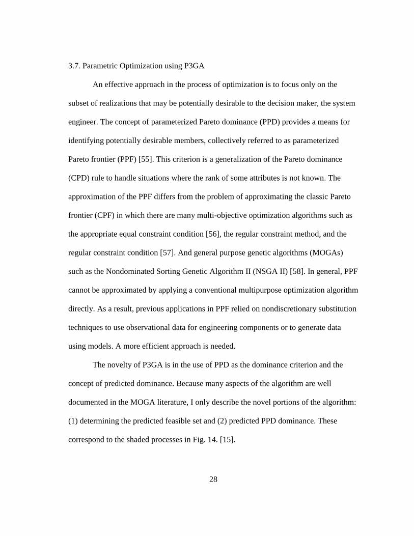
3.7. Parametric Optimization using P3GA
An effective approach in the process of optimization is to focus only on the
subset of realizations that may be potentially desirable to the decision maker, the system
engineer. The concept of parameterized Pareto dominance (PPD) provides a means for
identifying potentially desirable members, collectively referred to as parameterized
Pareto frontier (PPF) [55]. This criterion is a generalization of the Pareto dominance
(CPD) rule to handle situations where the rank of some attributes is not known. The
approximation of the PPF differs from the problem of approximating the classic Pareto
frontier (CPF) in which there are many multi-objective optimization algorithms such as
the appropriate equal constraint condition [56], the regular constraint method, and the
regular constraint condition [57]. And general purpose genetic algorithms (MOGAs)
such as the Nondominated Sorting Genetic Algorithm II (NSGA II) [58]. In general, PPF
cannot be approximated by applying a conventional multipurpose optimization algorithm
directly. As a result, previous applications in PPF relied on nondiscretionary substitution
techniques to use observational data for engineering components or to generate data
using models. A more efficient approach is needed.
The novelty of P3GA is in the use of PPD as the dominance criterion and the
concept of predicted dominance. Because many aspects of the algorithm are well
documented in the MOGA literature, I only describe the novel portions of the algorithm:
(1) determining the predicted feasible set and (2) predicted PPD dominance. These
correspond to the shaded processes in Fig. 14. [15].

29
Figure 14. Flow chart of the P3GA, Adapted from [15]
Because the application of PPD alone makes it difficult to predict the dominance
of all members, dominance analysis is performed not by relying on individual members
of the population, but those that are expected to be feasible. To predict what is feasible,
the observed points are used. The points that are dominated by the members of the
predictable feasible set are the predicted dominant points. To determine the predictable
set, P3GA relies on the SVDD technique [59], which models the outer boundary of the
current population in the combined variable space of the objective and the parameter.
Fig.15 shows the predicted parameterized dominance.

30
Figure 15. An illustration of predicted dominance, Adapted from [60]
The discrete set of points in the Pareto frontier is parameterized in the output of
P3GA. I normalize the data using Kriging interpolation to fit the model of the
parameterized Pareto Frontier in the combined space of the property space, the design
goal and the parameter variable. Fitting models must be in proper sequence and
mathematical form, or interpolated as in Kriging [60,61]
31
4. RESULTS
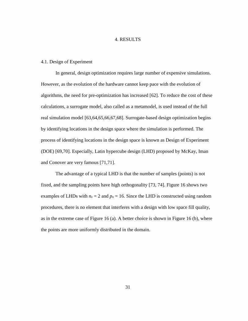
4.1. Design of Experiment
In general, design optimization requires large number of expensive simulations.
However, as the evolution of the hardware cannot keep pace with the evolution of
algorithms, the need for pre-optimization has increased [62]. To reduce the cost of these
calculations, a surrogate model, also called as a metamodel, is used instead of the full
real simulation model [63,64,65,66,67,68]. Surrogate-based design optimization begins
by identifying locations in the design space where the simulation is performed. The
process of identifying locations in the design space is known as Design of Experiment
(DOE) [69,70]. Especially, Latin hypercube design (LHD) proposed by McKay, Iman
and Conover are very famous [71,71].
The advantage of a typical LHD is that the number of samples (points) is not
fixed, and the sampling points have high orthogonality [73, 74]. Figure 16 shows two
examples of LHDs with nv = 2 and pn = 16. Since the LHD is constructed using random
procedures, there is no element that interferes with a design with low space fill quality,
as in the extreme case of Figure 16 (a). A better choice is shown in Figure 16 (b), where
the points are more uniformly distributed in the domain.

32
(a) (b)
Figure 16. Examples of Latin Hypercube Designs, Adapted from [74]
Based on these advantages, in the optimization, the 1st generation of p3ga, which
was formed randomly until now, was created by using LHD.
The utility of LHD is clearly observed when comparing the first generation of
DOE and optimization. As shown in Fig.17, when the initial points are selected
randomly, the distribution of each section is jagged. On the other hand, when LHD is
selected, the parameters are uniformly spread over all sections. The scattered plot of last
generation is shown in Fig.18. The difference of convergence is clearly observed.

33
Figure 17. Distribution of Experimental Points (First Generation), Design of
Experiment (TOP), Optimization (BOTTOM)
Figure 18. Experimental Points (25th Generation), H1 vs CD
02468
1012
< 0.1 >0.1 &<0.2
>0.2 &<0.3
>0.3 &<0.4
>0.4 &<0.5
>0.5 &<0.6
>0.6 &<0.7
>0.7 &<0.8
>0.8 &<0.9
>0.9 &<1.0
Nu
mb
er o
f C
ases
Normarlized Value
H1 L1 L2 KR1 KR2 d w
0
2
4
6
< 0.1 >0.1 &<0.2
>0.2 &<0.3
>0.3 &<0.4
>0.4 &<0.5
>0.5 &<0.6
>0.6 &<0.7
>0.7 &<0.8
>0.8 &<0.9
>0.9 &<1.0
Nu
mb
er o
f C
ases
Normailized Value
H1 L1 L2 KR1 KR2 d w
0.00E+00
1.00E-01
2.00E-01
3.00E-01
4.00E-01
5.00E-01
6.00E-01
7.00E-01
0.6 0.7 0.8 0.9 1 1.1 1.2 1.3 1.4
CD
H1 (m)
Optimization 1 Optimization 2

34
4.2. Validation of Models
4.2.1. Submarine Validation for Mesh
In order to investigate the effect of meshing on the performance of the submarine
prior to the full optimization, simulation was performed using the actual submarine
model. The base submarine model is a 1/10 scale Typhoon class model, as shown in
Fig.19.
Figure 19. Base Model – 1/10 Scale Typhoon Type Submarine
35
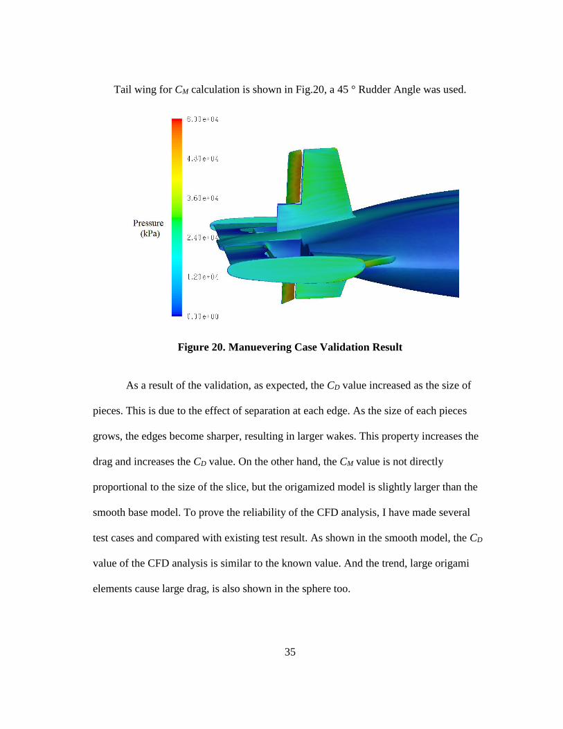
Tail wing for CM calculation is shown in Fig.20, a 45 ° Rudder Angle was used.
Figure 20. Manuevering Case Validation Result
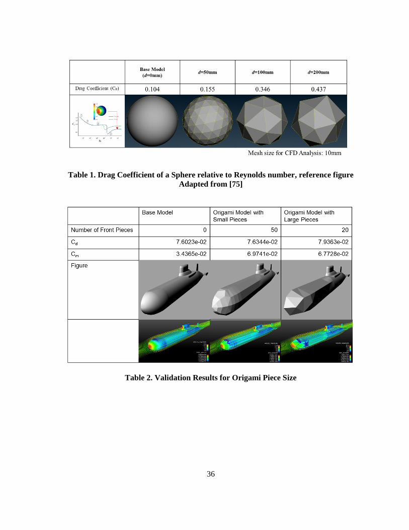
As a result of the validation, as expected, the CD value increased as the size of
pieces. This is due to the effect of separation at each edge. As the size of each pieces
grows, the edges become sharper, resulting in larger wakes. This property increases the
drag and increases the CD value. On the other hand, the CM value is not directly
proportional to the size of the slice, but the origamized model is slightly larger than the
smooth base model. To prove the reliability of the CFD analysis, I have made several
test cases and compared with existing test result. As shown in the smooth model, the CD
value of the CFD analysis is similar to the known value. And the trend, large origami
elements cause large drag, is also shown in the sphere too.
36
Table 1. Drag Coefficient of a Sphere relative to Reynolds number, reference figure
Adapted from [75]
Table 2. Validation Results for Origami Piece Size

37
4.2.2. Tail Wing
Before performing the simulation, I performed validation for tail wing selection,
which will be commonly attached to all models. Two types of tail wings used in the
validation is shown in Fig.21. The tail wing of type an exhibited a lower CD value but
was excluded from this optimization because it is accompanied by the roll direction
maneuver during yaw direction maneuver, which is the focus of this study.

38
Figure 21. Two Types of Tail Wings for Validation. A-Type (Top) And B-Type
(Bottom)
39
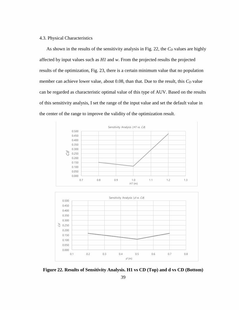
4.3. Physical Characteristics
As shown in the results of the sensitivity analysis in Fig. 22, the CD values are highly
affected by input values such as H1 and w. From the projected results the projected
results of the optimization, Fig. 23, there is a certain minimum value that no population
member can achieve lower value, about 0.08, than that. Due to the result, this CD value
can be regarded as characteristic optimal value of this type of AUV. Based on the results
of this sensitivity analysis, I set the range of the input value and set the default value in
the center of the range to improve the validity of the optimization result.
Figure 22. Results of Sensitivity Analysis. H1 vs CD (Top) and d vs CD (Bottom)
0.000
0.050
0.100
0.150
0.200
0.250
0.300
0.350
0.400
0.450
0.500
0.7 0.8 0.9 1.0 1.1 1.2 1.3
Cd
H1 (m)
Sensitivity Analysis (H1 vs Cd)
0.000
0.050
0.100
0.150
0.200
0.250
0.300
0.350
0.400
0.450
0.500
0.1 0.2 0.3 0.4 0.5 0.6 0.7 0.8
Cd
d (m)
Sensitivity Analysis (d vs Cd)
40
One unusual point in Fig. 23 is that all the test points appear above a certain CD
value. This phenomenon is due to the influence of the CD value on the Reynolds number,
as shown in Table.1. This simulation has a range of Re = 106 ~ 107 because v = 5 m/s and
water are assumed as mentioned above. Therefore, the sphere of the range has a CD
value of about 0.2 and the minimum CD value of about 0.1 for a streamlined AUV. In
addition, the reason for the flat result rather than the plot with a positive slope is that the
Cd value is inversely proportional to the projected area, and the projected area is again
proportional to H12. As shown in Fig. 23, the result of which is relatively proportional
than Fig. 24 is generated. As shown in Fig.24, the Drag Force is proportional to H12.
However, as the H1 value increases, the size of the area also increases, and a trade-off
occurs between the drag force and the Available Area. Based on this result, in
Optimization, Range other than the available area or CD was selected as one objective.

41
Figure 23. Projected Scatter Plot of All Populations: H1 vs. CD (Top) and d Vs. CD
(Bottom)

42
Figure 24. Projected Scatter Plot of All Populations: H1 vs. Drag Force
Tendency between available Area for solar panel and d, is not clear. However, the
number of data point with 0 available Area is decreased as the d increases. In the same
manner, tendency between w and Area is not clear. As shown in Figure 25, there is no
observable correlation between w (the fold width), and Area.
Figure 25. Projected Scatter Plot of All Populations w vs. Area
0
5
10
15
20
25
30
0.1 0.15 0.2 0.25 0.3 0.35 0.4 0.45
Are
a(m
2)
w

43
Figure 26. Projected Scatter Plot of All Populations d vs. Area
Similar to the results from sensitivity analysis, tendency between H1 and CM is
clearly negative. As shown in Fig.26, H1 increases, controllability of AUV decreases.
This is caused by difference of projected area. H1 increases both frontal projection area
and side projection area. Both areas affect CM. Since all the cases shared same tail wings,
higher CM means higher controllability through moment force.
0
5
10
15
20
25
30
0 0.1 0.2 0.3 0.4 0.5 0.6 0.7 0.8
Area
(m^2
)
d (m)
Figure 27. Results of H1 vs. CM grom Sensitivity Analysis (Top) and Projected
Scatter Plot (Bottom)

44
From Optimization, as shown in Fig. 27, tendency between the parameter H1 and
inner volume and range were brought to light. As expected, inner volume is directly
proportional to H1. In contrast, the relation between range and H1 is not clearly
observable as also shown in Fig. 27. Here, the dots in different colors represent the
experimental points of the last generation. The distributions are spread over a wide range
but show linear results. This is due to the fact that the range is broad because it is
projected, but it is close to the formed Pareto front as shown in the three-dimensional
plot.
0
0.05
0.1
0.15
0.2
0.25
0.6 0.7 0.8 0.9 1 1.1 1.2 1.3 1.4
Cm
H1 (m)
Figure 27. Continued

45
Figure 28. Projected Scatter Plot of all Populations H1 vs. Inner Volume (Top) and
H1 vs Range (Bottom)
Figure. 28 shows the projected plot of available inner volume vs. range and their
associated Pareto frontier. Range is directly related with the available area for solar cells
for solar cells. In contrast, available area and inner volume are inversely proportional
due to hidden surfaces. That is the reason that projected Pareto front displays a negative
slope. The parameterized Pareto points, shown in bottom of Fig.28, the trend due to H1
0
0.5
1
1.5
2
2.5
3
3.5
4
0.6 0.7 0.8 0.9 1 1.1 1.2 1.3 1.4
Inn
er V
olu
me
(m2)
H1 (m)
0
2000
4000
6000
8000
10000
12000
14000
0.6 0.7 0.8 0.9 1 1.1 1.2 1.3 1.4
Ra
ng
e(m
)
H1 (m)

46
is clearly observed. As the H1 increases, Available Inner Volume increase while the
Range decreases. This is due to the trade-off between hydrodynamically efficient shape
and large inner volume.
Figure 29. Projected Scatter Plot for Range vs Inner Volume of all Populations
(TOP) and Non-dominated Populations (BOTTOM)
0
0.5
1
1.5
2
2.5
3
3.5
4
0.6 2000.6 4000.6 6000.6 8000.6 10000.6 12000.6 14000.6
Ava
ilab
le I
nn
er
Vo
lum
e (m
3)
Range (m)
0.5
1
1.5
2
2.5
3
0 2000 4000 6000 8000 10000 12000 14000
Ava
ilab
le I
nn
er
Vo
lum
e (m
3)
Range (m)
H1 <1.0 1.0 < H1 < 1.1 1.1 < H1 < 1.2 1.2 < H1

47
Three objectives and one unknown parameter are considered in Design of
Experiment. Therefore, the Pareto frontier forms a surface in three-dimensional space.
As shown in Fig. 29, the ranges of scattered points are wide for all objectives. However,
the three-dimensional Pareto surface, shown in Fig. 30, is formed in a small range. This
is because design points located at the boundaries exhibited desirable results for one of
the objectives but not for the others. Another issue to consider from the results is zero
available solar cell area for several cases. If the area of each mesh is too small to attach a
single solar cell, then the available area is set to zero for the mesh. That is the reason
why many points are located on the 0 area line. As shown in Fig. 30, this happened in
optimization again as 0 range scattered points.
Figure 30. Three-Dimensional Scatter Plot of all Populations for Design of
Experiment
4.4. Pareto Front

48
Figure 31. Three-Dimensional Pareto Frontiers for Design of Experiment
For the optimization, dependence toward the uncertain parameter H1 is clarified in
Fig. 31 and Fig. 32. Similar to the results from Fig. 26, H1 and the available inner
volume are dependent. And for all parameter, trade-off between two objectives is
observed. The feature of the pareto front is that it is not a surface with a gentle slope but
a surface with a large slope where the Inner Volume changes abruptly. This is due to the
difference in the influence of the w value. The available Inner Volume changes greatly
depending on the value of w, but the change of the Range is not large, and this
phenomenon occurs. As you can see from Fig. 30, the reason why you can show a high
range value at the middle value H1 than the maximum and minimum values is due to the
range of L1 and L2 values in Optimization # 2. If L1 and L2 values are not limited, the
Range decreases and the available Inner Volume increases as the H1 value increases.

49
Figure 32. Three Dimensional Pareto Frontiers via Interpolated Mesh for
Optimization
Figure 33. Three Dimensional Scatter Plot of each Unknown Parameter (H1) for
Optimization
0
0.5
1
1.5
2
2.5
3
3.5
4
0 2000 4000 6000 8000 10000 12000 14000
Ava
ilab
le I
nn
er V
olu
me
(m^2
)
Range (m)
0.7 < H1 < 0.9 0.9 < H1 < 1.0 1.0 < H1 < 1.1 1.1 < H1 < 1.3

50
First and most importantly, I have to gather data and proceed optimization. In
consequence of sensitivity analysis, parametric range is decided. Constraints and
baseline of the model are decided with a reference to Jalbert’s paper [17]. Currently it
takes five to seven minutes per case. But since three-dimensional modeling, CFD
analysis and origami can run at the same time, it can be reduced to 2 to 3 minutes per
case with a set of data which is one generation of Genetic Algorithm.
Final goal is to build a high quality model and compare with high quality baseline
model where the optimization is started. This high quality model can be also used for 3D
printing that I can embark experiment with real model in the future.

51
5. CONCLUSIONS
In this thesis, a design framework for an AUV with origami morphing capabilities
was proposed and demonstrated. The present origami design method is applicable to the
AUV because its outer shape can be represented as a 2-manifold, orientable surface
topologically equivalent to a disk. The novel origami-based design of the AUV proposed
here allows the folding and unfolding of the vehicle between the AUV shape optimized
for hydrodynamic efficiency (to navigate underwater and store materials) and the planar
shape (that maximizes the projected area of the AUV solar panels to charge the power
supplies). The AUV designs were evaluated using several software and tools such as
ANSYS, Rhinoceros, and in-house codes for origami design. In this particular case, I
have focused on optimizing parameters associated with mission range and mobility.
Future work will consider other physical characteristics that might be critical to the AUV
performance. The folding simulation of the AUV used here only considers kinematics
(i.e., the constitutive response of the materials potentially comprising the folds is not
considered). Future work will include the consideration of the constitutive response of
the active materials (e.g., shape memory alloys or shape memory polymers) that will
potentially comprise the folds.
AUV, as an unmanned underwater vehicle, simulated hydrodynamic performance
depending on the variables were line with expectations. Minimum drag coefficients (CD)
were 0.08 which is the lowest value that the streamlined shape can achieve. In addition,
trade-off between available area (Area) and available inner volume (Volume) is observed
clearly. Influence of unknown parameter, H1, is also clearly observed.

52
REFERENCES
[1] Zirbel, Shannon A., et al. "An origami-inspired self-deployable array." ASME 2013
Conference on Smart Materials, Adaptive Structures and Intelligent Systems. American
Society of Mechanical Engineers, 2013.
[2] Tachi T. “Geometric considerations for the design of rigid origami structures.” In:
Proceedings of the International Association for Shell and Spatial Structures (IASS)
Symposium. Vol. 12; 2010. p. 458–460.
[3] Wu W., You Z. “Modelling rigid origami with quaternions and dual quaternions.”
Proceedings of the Royal Society of London A: Mathematical, Physical and Engineering
Sciences. 2010;466(2119):2155–2174.
[4] Liu S., Chen Y., Lu G. “The rigid origami patterns for flat surface.” In: ASME
DETC/CIE 2013. American Society of Mechanical Engineers; 2013. p. DETC2013–
12947, pp. V06BT07A039.
[5] Evans T., Lang R., Magleby S., Howell L. “Rigidly foldable origami gadgets and
tessellations.” Royal Society Open Science. 2015;2(9).
[6] Zhou X., Wang H., You Z. “Design of three-dimensional origami structures based on
a vertex approach.” Proceedings of the Royal Society of London A: Mathematical,
Physical and Engineering Sciences. 2015;471(2181):20150407.
[7] Bowers J. “Skeleton structures and origami design.” Thesis, University of
Massachusetts, Amherst. 2015.
[8] Tachi T. “Simulation of rigid origami.” Origami 4, Fourth International Meeting of
Origami Science, Mathematics, and Education. 2009; p. 175–187.
[9] Filipov E., Paulino G., Tachi T. “Origami tubes with reconfigurable polygonal cross-
sections.” Proceedings of the Royal Society of London A: Mathematical, Physical and
Engineering Sciences. 2016;472(2185):20150607.
[10] Dudte L. H., Vouga E., Tachi T., Mahadevan L. “Programming curvature using
origami tessellations.” Nature Materials. 2016;15(5):583–588.
[11] Dureisseix D. “An overview of mechanisms and patterns with origami.”
International Journal of Space Structures. 2012;27(1):1–14.
[12] Gattas J., You Z. “Miura-base rigid origami: parametrizations of curved-crease
geometries.” Journal of Mechanical Design. 2014;136(12):121404.

53
[13] Husaini, M., Samad, Z., Arshad, M. “Autonomous underwater vehicle propeller
simulation using computational fluid dynamic”, Computational Fluid Dynamics
Technologies and Applications, InTech, pp. 293–314, 2011.
[14] Khairul, A., Ray, T., and Anavatti, S. “Design and construction of an autonomous
underwater vehicle.” Neurocomputing, 142: 16-29, 2014.
[15] McCartney, B. S., and P. G. Collar. "Autonomous submersibles-instrument
platforms of the future.",1989.
[16] Ageev, M. “An analysis of long-range AUV, powered by solar energy.”
OCEANS'95. MTS/IEEE. Challenges of Our Changing Global Environment.
Conference Proceedings. Vol. 2. IEEE, 1995.
[17] Lutz, T. and Wagner, S. “Numerical shape optimization of natural laminar flow
bodies.” In: Proceedings of the 21st ICAS congress, Melbourne, Australia, pp.1–11,
1998.
[18] Bertram V. and Alvarez A., “Hydrodynamic aspects of AUV design”, 5th
conference on computer and IT applications in the maritime industries (COMPIT),
Oegstgeest, Netherlands, pp. 45–53,2006.
[19] Alvarez, A, Bertram, V. and Gualdesi, L., “Hull hydrodynamic optimization of
autonomous underwater vehicles operating at snorkeling depth” Ocean Eng., 36:105–
112, 2009.
[20] Phillips, A., Turnock, S., and Furlong, M., “The use of computational fluid
dynamics to aid cost-effective hydrodynamic design of autonomous underwater
vehicles” Proc IMechE Part M: J Engineering for the Maritime Environment, 224: 239–
254, 2010.
[21] Stevenson P., Furlong M. and Dormer D., “AUV shapes combining the practical
and hydrodynamic considerations”, In: Proceedings of the OCEANS 2007 Europe
MTS/IEEE conference and exhibition, Aberdeen, UK, pp.1–6, 2007.
[22] Joung, T., Sammut, K., He, F. and Lee, S., “A study on the design optimization of
an AUV by using computational fluid dynamic analysis” In: Proceedings of the 19th
international offshore and polar engineering conference, Osaka, Japan, pp. 696–702,
2009.
[23] Khairul, A., Ray, T., and Anavatti, S. “A new robust design optimization approach
for unmanned underwater vehicle design.” Proceedings of the Institution of Mechanical
Engineers, Part M: Journal of Engineering for the Maritime Environment, 226.3: 235-
249, 2012.
54
[24] Samareh, J. “A Survey of Parameterization Techniques”,
CEAS/AIAA/ICASE/NASA Langley International Forum on Aeroelasticity and
Structural Dynamics, Williamsburg, VA, pp. 333–343, 1999.
[25] Piegl, L., and Tiller, W. The NURBS Book, Springer, New York, 1997.
[26] Piegl, L. “On NURBS: a Survey”, IEEE Computer Graphics and Applications,
Volume 11 Issue 1, Page 55-71, January 1991.
[27] Hur, D. “Ground vehicle optimization regarding aesthetic completeness and
aerodynamic characteristics by modification of vehicle modeling function and
conceptual design process”, 51st AIAA Aerospace Sciences Meeting including the New
Horizons Forum and Aerospace Exposition, Grapevine (Dallas/Ft. Worth Region),
Texas, January 2013.
[28] Peraza Hernandez, E., Hartl, D., Akleman, E., and Lagoudas, D. "Modeling and
analysis of origami structures with smooth folds." Computer-Aided Design, 78, pp. 93-
106, 2016.
[29] Peraza Hernandez, E., Hartl, D., Lagoudas D. “Design of origami structures with
smooth folds.” In ASME 2016 Conference on Smart Materials, Adaptive Structures and
Intelligent Systems, 2016, p. V002T03A018.
[30] Peraza Hernandez, E., Hartl, D., and Lagoudas, D., “Kinematics of origami
structures with smooth folds.” Journal of Mechanisms and Robotics, 8(6), 2016,
p.061019.
[31] Peraza Hernandez, EA, D. J. Hartl, and D. C. Lagoudas. "Design and simulation of
origami structures with smooth folds." In Proc. R. Soc. A, vol. 473, p. 20160716. The
Royal Society, 2017.
[32] H.A. Taha, Operations Research: An Introduction (For VTU), 8th edn. Pearson
Education India, 1982.
[33] P.Y. Papalambros, D.J. Wilde, “Principles of optimal design: modeling and
computation”, Cambridge university press, 2000.
[34] T.C. Wagner, P.Y. Papalambros, “Selection families of optimal engine designs
using nonlinear programming and parametric sensitivity analysis”, Tech. rep., SAE
Technical Paper, 1997.
[35] Jalbert, J. "A solar-powered autonomous underwater vehicle." Oceans 2003.
Proceedings. Vol. 2. IEEE, 2003.

55
[36] Blidberg, Ageev, and Jalbert, “Some Design Considerations for a Solar Powered
AUV; Energy Management and its Impact on Operational Characteristics”, Unmanned
Untethered Submersible Technology Sept. 7-10, 1997.
[37] Calkins, D., and Chan, W. “CD aero - A parametric aerodynamic drag prediction
tool”, International Congress and Exposition, Detroit, MI, SAE Paper No. 980398, 1998.
[38] Tovey, M. “Computer-aided vehicle styling,” Comput. Aided Des, 21(3), pp. 172–
179, 1989.
[39] Lyu, N., and Saitou, K. “Decomposition-based assembly synthesis of space frame
structures using joint library,” ASME J. Mech. Des., 128, pp. 57–65, 2006.
[40] Lo, S. “A new mesh generation scheme for arbitrary planar domains”, Int. J.
Numer. Methods Eng., 21:1403–1426 ,1985.
[41] Zhu, J. Z., Zienkiewicz, O. C., Hinton, E., Wu, J. “A new approach to the
development of automatic quadrilateral mesh generation” Int. J. Numer. Methods Eng.,
32:849–866, 1991.
[42] Johnston, B. P., Sullivan, J. M. “A normal offsetting technique for automatic mesh
generation in three dimensions” Int. J. Numer. Methods Eng., 36:1717–1734, 1993.
[43] Jin, H., Tanner, R. I., “Generation of unstructured tetrahedral meshes by advancing
front technique”, Int. J. Numer. Methods Eng., 36:1805–1823, 1993.
[44] George, P. L., Seveno, E. “The advancing-front mesh generation method revisited”,
Int. J. Numer. Methods Eng., 37:3605–3619, 1994.
[45] Mavriplis, D. "An advancing front Delaunay triangulation algorithm designed for
robustness." 31st Aerospace Sciences Meeting. 1992.
[46] Launder, Brian Edward, and Dudley Brian Spalding. "Lectures in mathematical
models of turbulence." 1972.
[47] Fluent, Ansys. "12.0 Theory Guide.", Ansys Inc 5, 2009.
[48] Schlichting, Hermann, et al. Boundary-layer theory. Vol. 7. New York: McGraw-
hill, 1960.
[49] Wilcox, David C. Turbulence modeling for CFD. Vol. 2. La Canada, CA: DCW
industries, 1998.
56
[50] Bardina, J., et al. "Turbulence modeling validation." 28th Fluid dynamics
conference. 1997.
[51] BYD North America Headquarters, 1800 S. Figueroa Street, Los Angeles,
CA90015, USA, Tel: +1-213-748-3980
[52] EcoDirect, 2834 La Mirada Drive, Suite E Vista, CA 92081
[53] Tachi, Tomohiro. "Origamizing polyhedral surfaces." IEEE transactions on
visualization and computer graphics 16.2 (2010): 298-311.
[54] Robert McNeel & AssociatesSeattle Weather, Headquarters, North America, and
Pacific 3670 Woodland Park Ave N, Seattle, WA 98103 USA.
[55] Malak, R. J., and Paredis, C. J. J., 2010, “Using Parameterized Pareto Sets to Model
Design Concepts,” ASME J. Mech. Des., 132(4), p. 041007.
[56] Lin, J. G., 1976, “Multiple-Objective Problems: Pareto-Optimal Solutions by
Method of Proper Equality Constraints,” IEEE Trans. Autom. Control, 21(5),pp. 641–
650.
[57] Messac, A., and Mattson, C. A., 2004, “Normal Constraint Method With Guarantee
of Even Representation of Complete Pareto Frontier,” AIAA J., 42(10), pp. 2101–2111.
[58] Deb, K., Pratap, A., Agarwal, S., and Meyarivan, T., “A Fast and Elitist Multi-
objective Genetic Algorithm: NSGA-II,” IEEE Trans. E vol. Comput., 6(2), pp. 182–
197, 2002.
[59] Tax, David MJ, and Robert PW Duin. "Support vector domain description." Pattern
recognition letters 20.11 (1999): 1191-1199.
[60] Hartl, Darren J., et al. "Parameterized design optimization of a
magnetohydrodynamic liquid metal active cooling concept." Journal of Mechanical
Design 138.3 (2016): 031402.
[61] Van Beers, Wim CM, and Jack PC Kleijnen. "Kriging interpolation in simulation: a
survey." Simulation Conference, 2004. Proceedings of the 2004 Winter. Vol. 1. IEEE,
2004.
[62] Venkataraman S, and Haftka RT, “Structural optimization complexity: what has
Moore’s law done for us?”, Structural and Multidisciplinary Optimization, Vol. 28, No.
6, pp. 375-387, 2004.
57
[63] Sacks J, Welch WJ, Mitchell TJ, and Wynn HP, Design and Analysis of Computer
Experiments, Statistical Science, Vol. 4 (4), pp. 409-435, 1989.
[64] Simpson TW, Peplinski JD, Koch PN, and Allen JK, Meta-models for computer
based engineering design: Survey and recommendations. Engineering with Computers,
Vol. 17, No. 2, pp. 129-150, 2001.
[65] Queipo NV, Haftka RT, Shyy W, Goel T, Vaidyanathan R, and Tucker, PK,
Surrogate-based analysis and optimization, Progress in Aerospace Sciences, Vol. 41, pp.
1-28, 2005.
[66] Simpson TW, Toropov V, Balabanov V, and Viana FAC, Design and Analysis of
Computer Experiments in Multidisciplinary Design Optimization: a Review of How Far
We Have Come – or Not, in: Proceedings of the 12th AIAA/ISSMO Multidisciplinary
Analysis and Optimization Conference, Victoria, Canada, September 10-12, 2008.
AIAA 2008-5802.
[67] Kleijnen JPC, Design and analysis of simulation experiments, Springer Verlag,
2007.
[68] Forrester AIJ and Keane AJ, Recent advances in surrogate-based optimization,
Progress in Aerospace Sciences, Vol. 45, No. 1-3, pp. 50-79, 2009.
[69] Montgomery DC, Design and analysis of experiments, John Wiley & Sons, 2004.
[70] Simpson TW, Lin DKJ, and Chen W, Sampling Strategies for Computer
Experiments: Design and Analysis, International Journal of Reliability and Applications,
Vol. 2, No. 3, pp.209-240, 2001.
[71] McKay MD, Beckman RJ, and Conover WJ, A Comparison of Three Methods for
Selecting Values of Input Variables from a Computer Code, Technometrics, Vol. 21, pp.
239-245, 1979.
[72] Iman RL, and Conover WJ, Small sample sensitivity analysis techniques for
computer models, with an application to risk assessment, Communications in Statistics,
Part A. Theory and Methods, Vol. 17, pp. 1749-1842, 1980.
[73] Kleijnen JPC, Sanchez SM, Lucas TW, and Cioppa TM, A user’s guide to the brave
new world of designing simulation experiments, INFORMS Journal on Computing, Vol.
17, No. 3, pp. 263-289, 2005.
[74] Bates, Stuart J., Johann Sienz, and Vassili V. Toropov. "Formulation of the optimal
Latin hypercube design of experiments using a permutation genetic algorithm." AIAA
Paper, 2004-2011, 2004: 1-7.

58
[75] "Drag of a Sphere." NASA. NASA, 05 May 2015. Web. 05 June 2017.
Recommended