Demand Fluctuations and Plant Turnover inthe Ready-Mix Concrete Industry
Allan Collard-Wexler∗
NYU
December 13, 2006
Abstract
Fluctuations in demand cause some plants to exit a market andother to enter. Would eliminating these fluctuations reduce plant turnover?A structural model of entry and exit in concentrated markets is es-timated for the ready-mix concrete industry, using plant level datafrom the U.S. Census. The Nested Pseudo-Likelihood algorithm isused to find parameters which rationalize behavior of firms involvedin repeated competition. Due to high sunk costs, turnover rates wouldonly be reduced by 3% by eliminating demand fluctuations at the
∗The work in this paper is drawn from chapter 2 of my Ph.D. dissertation at North-western University under the supervision of Mike Whinston, Rob Porter, Shane Greensteinand Aviv Nevo. I would like to thank Lynn Riggs, Mike Mazzeo and Ambarish Chandrafor helpful conversations, the Fonds Quebecois de la Recherche sur la Societe et la Cul-ture (FQRSC) and the Center for the Study of Industrial Organization at NorthwesternUniversity (CSIO) for financial support. I would like to thank seminar participants atNorthwestern University, Chicago GSB, Yale University, Western Ontario, University ofWisconsin-Madison, University of Minnesota, Stanford University, UCLA, UCSD, NYU,Columbia, Princeton, Harvard Business School, HEC-Montreal, University of Montreal,Concordia University, UQAM and the Chicago Federal Reserve Bank for comments. Theresearch in this paper was conducted while I was a Special Sworn Status researcher of theU.S. Census Bureau at the Chicago Census Research Data Center. Research results andconclusions expressed are those of the author and do not necessarily reflect the views of theCensus Bureau. This paper has been screened to insure that no confidential data are re-vealed. Support for this research at the Chicago RDC from NSF (awards no. SES-0004335and ITR-0427889) is also gratefully acknowledged.
1

county level, saving around 20 million dollars a year in scrapped cap-ital. However, demand fluctuations blunt firms’ incentive to invest,reducing the number of large plants by more than 50%.
1 Introduction
Many industries face considerable uncertainty about future demand for their
products, perhaps most universally because of aggregate fluctuations in eco-
nomic activity due to the business cycle. These fluctuations are costly, since
firms change their production process to suit the current level of demand,
hiring and firing workers, purchasing and scraping machinery, opening and
shutting down plants. In this paper, I focus on a single industry, ready-mix
concrete, and a specific type of adjustment central to industrial economics,
plant entry and exit, to evaluate the cost of demand fluctuations.
The ready-mix concrete industry is unusually well suited to study the
impact of fluctuations in demand on entry and exit and industry structure.
The concrete industry witnesses large changes in output from year to year as
illustrated by Figure 1, which are of great concern to ready-mix producers.
These fluctuations are caused in part by the effect of changes in interest
rates on new construction activity, and variation in government spending
on highways and buildings. Moreover, there is substantial regional and local
variation in construction activity, that affects ready-mix plants within only
a limited area due to high transportation costs. Indeed, wet concrete cannot
travel for much more than an hour before it hardens in the barrel of a truck.
2

Cement Consumption and Construction Employment 1976-1999
5.5
6
6.5
7
7.5
8
8.5
1976
1977
1978
1979
1980
1981
1982
1983
1984
1985
1986
1987
1989
1990
1991
1992
1993
1994
1995
1996
1997
1998
1999
Mill
ion
tons
of C
emen
t
70
80
90
100
110
120
130
Bill
ion
dolla
rs o
f sal
arie
s (d
efla
ted)
Cement Consumption (left)Construction Payroll (right)
Figure 1: Cement consumption (used in fixed proportion to concrete) andconstruction sector salaries are very procyclical and volatile.
3

There is considerable plant turnover in the ready-mix concrete industry.
In a five year period more than 30% of plants will shut down and 30% of
plants will be born. Moreover, entry and exit are responsible for 15% of jobs
created and destroyed. Would dampening fluctuations in demand for concrete
from the construction sector reduce job and plant turnover? What is the cost
to society of this turnover? Moreover, is industry composition substantially
altered by these demand fluctuations?
I answer these questions with longitudinal data provided by the Cen-
ter for Economic Studies at the Census Bureau, on the life histories of over
15 000 ready-mix concrete plants in United States from 1963 to 2000. These
data provided detailed information on the inputs and outputs of plants as
well as on entry and exit. I estimate a model of dynamic competition in
concentrated markets using the Nested Pseudo-Likelihood algorithm (NPL)
developed by Aguirregabiria and Mira (2006), that identifies the parameters
of the dynamic game firms play from their equilibrium strategies. Moreover,
I incorporate market level fixed effects into this model to control for persis-
tent, but unobserved, differences between markets. I cannot, however, use a
static model of entry and exit, such as the models of Bresnahan and Reiss
(1994), since these are incapable of performing the counterfactual: a perma-
nent change in the volatility of demand. Instead, a fully dynamic, multi-agent,
model is required.
I find that a ready-mix concrete plant entails substantial sunk costs. My
estimates indicate that a potential entrant is indifferent between a permanent
4

monopoly market and a permanent duopoly market where she would not have
to pay sunk costs.
The econometric model is used to simulate the effect of eliminating yearly
changes in demand at the county level. I find that plant turnover would be
only 3% lower in a world without demand fluctuations. This number is quite
small, implying that 20 million dollars a year is lost due to unnecessary
plant shut down and opening, i.e. plant turnover which would not exist in
the absence of demand fluctuations. Because of large sunk costs, plants are
unlikely to exit during a temporary lull in demand. Sunk costs slow the
reaction of firms to short-run fluctuations in demand, since it is costly to
build new plants or to shut down old ones. Thus, high entry and exit rates
in ready-mix concrete must stem from idiosyncratic shocks to firm profits,
caused by a myriad of factors such as mergers and productivity.
However, focusing on industry turnover misses the impact of demand
fluctuations on industry composition. Demand uncertainty blunts firms in-
centives to invest. Eliminating fluctuations increases the number of large
plants (above 15 employees) in the industry by more than 50%. Firms are
more likely to build larger, more productive plants if they can be assured
that there will be continuing demand for their products.
In section 2, I discuss the source of sunk costs for the Ready-Mix Plants,
and the role of spatial differentiation in the industry. Section 3 describes how
I construct the data. In section 4, I present a dynamic model of competition,
and I describe estimation in section 5. Finally, in section 6 I discuss steady-
5

state industry dynamics predicted by the model for a world with demand
fluctuations and one where they have been removed. Some supplementary
Tables and Figures are collected in section A. 1
2 The Ready-Mix Concrete Industry
Concrete is a mixture of three basic ingredients: sand, gravel (crushed stone)
and cement, as well as chemical compounds known as admixtures. Combining
this mixture with water causes the cement to undergo an exothermic chemical
reaction called hydration, turning cement into a hard paste that binds the
sand and gravel together. I focus on ready-mix concrete: concrete which is
mixed with water at a plant and transported directly to a construction site. 2
Ready-Mix is a perishable product that needs to be delivered within an hour
and a half before it becomes too stiff to be workable. 3 Concrete is also very
cheap for its weight. One producer describes the economics of transportation
costs in the ready-mix industry as follows:
A truckload of concrete contains about 7 cubic yards of con-
crete. A cubic yard of concrete weights about 4000 pounds and
1Further robustness checks, details of the construction of the data set and computa-tional details can be found in Collard-Wexler (2006a), the web appendix to this paper.
2There are of course other types of concrete, such as bag concrete produced in smallbatches at a construction site, or pre-cast concrete products, such as septic tanks andpipes. These concrete products are neither substitutes for ready-mix concrete, nor arethey produced at ready-mix plants.
3 “ASTM C 94 also requires that concrete be delivered and discharged within 1 1/2hours or before the drum has revolved 300 times after introduction of water to the cementand aggregates” p.96 in Kosmatka, Kerkhoff, and Panarese (2002).
6

will cost you around $60 delivered to your door. That’s 1.5 cents
a pound. If you go to your local hardware store, you get a bag of
manure weighing 10 pounds for $5. That means that concrete is
cheaper than shit. 4
A ready-mix truck typically drives 20 minutes to deliver a load. 5 Thus,
concrete’s most salient feature from an economic perspective is that markets
are geographically segmented. Figure 2 shows the dispersion of ready-mix
producers in the Midwest, with an handful of incumbents in each area. In
my empirical work I treat each county as a separate market, one that evolves
independently from the rest of the industry.
Table A2 shows that the vast majority of counties in the United States
have fewer than 6 ready-mix plants, reflecting a locally oligopolistic market
structure. At the same time, because even the most isolated rural areas has
demand for ready-mix concrete, most counties are served by at least one
ready-mix producer.6
Ready-Mix concrete is essentially a homogeneous good. While it is possi-
ble to produce several hundred types of Ready-Mix concrete, these mixtures
basically use the same ingredients and machinery. Because of aggressive an-
titrust policy on the part of the Department of Justice, the typical ready-mix
4Telephone interview, January 2005.5The driving time of twenty minutes is based on a dozen interviews conducted with
Illinois ready-mix concrete producers. Thanks to Dick Plimpton at the Illinois Ready-MixConcrete Association for providing IRMCA’s membership directory.
6Isolated towns have also been used as a market definition, in the manner of Bresnahanand Reiss (1991) which are documented in Collard-Wexler (2005). Parameter estimatesfor a static entry model using isolated markets are similar to those using county markets.
7

��
��
��
�� ����
��
��
�� ����
��
��
��
����
��
��
����
��
��
��
����
��
��
��
����
��
��
��
��
�� �� ��
���� ����
��
����
����
��
��
����
��
��������
����
������ ��
��
����
��
��
������ ������
���� ����
��
��
���� ��
�������� ��
��������
����
������
��
����������
����
��
����
����
����
������
��
��
������
��
��
������ ��
��
��
��
��
��
��
��
��
��
��
��
����
������
��
�� ��
��
��
������ ����
����
��
��������
��
��
�� ����
��
��
��
��
��
����
����
��
��
��
��
��
��
����
��
����
��
��
��
��
��
��
����
��
��
��
��������
����
����
����
�� ��
��
�� ����
���� ���� ��
��
��
��
�� ��
����
���� ��
��
��
����
����
����
������
��
����
��
�� ����
����
��
��
�� ��
����
����
����
��
��
��
����
��
��
��
��
��
��
��
����
����
��
����
������
����
��
��
����
��
����
����
����
������
��
����
��
�� ����
����
��
����
�� ��
�� ������
��
������
����
��
����
������
����������������� ������������������ ��� ��� ��� ������� �����
��� � ��� ��� �����
Figure 2: Dispersion of Ready-Mix Plant Locations in the Midwest.Source: Zip Business Patterns publicly available dataset at
http://www.census.gov/epcd/www/zbp base.html.
8

producer is a single plant operator.7 Indeed, Syverson (2004) reports that
3749 firms controlled the 5319 ready-mixed plants operating in 1987. Thus I
will assume that each firm owns a single ready-mix concrete plant, making
plant and firm interchangeable.
Opening a concrete plant is an expensive investment. In interviews, man-
agers of ready-mix plants estimate the cost of a new plant costs at between
3 and 4 million dollars, while Table A7 in section A shows that continuing
plants in 1997 had on average 2 million dollars in capital assets. There are
few expenses involved in shutting down a ready-mix plant. Trucks can be
sold on a competitive used vehicle market, and land can be sold for other
uses. The plant itself is a total loss. At best it can be resold for scrap metal,
but many ready-mix plants are left on site because the cost of dismantling
them outweighs the benefits. An evocative illustration of capital’s sunkness
is Ramey and Shapiro (2001) study of the resale of capital assets at several
aerospace plants. Used capital sells for a fraction of its new value, even after
accounting for depreciation. I provide evidence of sunk costs in the ready-
mix industry at the plant level, including factors difficult to quantify, such
as long term relationships with clients and creditors. These intangible assets
may account for a large fraction of sunk costs. 8
7 The history of the Department of Justice’s policy toward mergers in the ready-mixconcrete industry is documented in McBride (1983).
8For instance, ready-mix operators sell about half of their production with a six monthgrace period for repayment. Accounts receivable have a value equivalent to half of a plant’sphysical capital assets. It will be more difficult to collect these accounts if the firm cannotpunish non-payment by cutting off future deliveries of concrete.
9

Concrete is consumed by the construction sector. Table A1 in section
A shows that the bulk of concrete purchases are made by the construction
sector, to build apartments, houses, roads and sidewalks. I use employment
in the construction sector as my demand measure. 9 Demand for ready-mix
concrete is inelastic since it is a small part of construction costs. Indeed, Table
A1 shows that concrete costs do not exceed 10% of material costs for any
construction sector. So it is unlikely that the ready-mix market substantially
affects the volume of construction activity. In addition Government purchases
about half of U.S. concrete, primarily for road construction.10 Fluctuations in
Government purchases of concrete are mainly due to the discretionary nature
of highway spending in state and federal budgets. Government purchases are
procyclical, and a major source of uncertainty for ready-mix producers.11
Ready-mix concrete has been studied extensively by Syverson (2004), who
provides evidence of productivity dispersion across plants. This productiv-
ity dispersion is evidence of large differences between plants which are not
eliminated by competitive pressures. I provide an explanation for why the
competitive adjustment process is not instantaneous.
9I have selected construction employment as my demand measure, out of a panoply ofmeasures of concrete demand such as: interest rates, construction payroll, employment inthe concrete contractor sector, area. I have used the static entry models of Bresnahan andReiss (1994) presented in Collard-Wexler (2005) to select the measure of demand whichaccounts for most of the differences between markets.
10 According to the Kosmatka, Kerkhoff, and Panarese (2002) p.9, Government accountsfor 48% of cement consumption, with road construction alone responsible for 32% of totalconsumption.
11Conversation with Edward Sullivan, chief economist at the Portland Cement Associ-ation, May 2005.
10

3 Data
Data on Ready-Mix Concrete plants is drawn from three different data sets
provided by the Center for Economics Studies at the United States Census
Bureau. Table 1 illustrates the datasets used. The first is the Census of Man-
ufacturing (henceforth CMF), a complete census of manufacturing plants,
every five years from 1963 through 1997. The second is the Annual Sur-
vey of Manufacturers (henceforth ASM) sent to a sample of manufacturing
plants (about a third for ready-mix) every non-Census year since 1973. Both
the ASM and the CMF involve questionnaires that collect detailed informa-
tion on a plant’s inputs and outputs. The third data set is the Longitudinal
Business Database (henceforth LBD) compiled from data used by the In-
ternal Revenue Service to maintain business tax records. The LBD covers
all private employers on a yearly basis since 1976. The LBD only contains
employment and salary data, along with sectoral coding and certain types
of business organization data such as firm identification. Construction data
is obtained by selecting all establishments from the LBD in the construction
sector (SIC 15-16-17) and aggregating them to the county level.
CMF ASM LBDData Set Census of Manufacturing Annual Survey of Manufacturing Longitudinal Business DatabaseCollection Questionnaire Questionnaire IRS Tax DataYears 1963, 67, 72, 77, 82, 87, 92, 97 1972-2000 1976-1999Coverage All Manufacturing Firms 30% of Manufacturing Firms All Private Sector FirmsVariables Input and Output Data including Input and Output Data Employment and Payroll
materials and product trailers and Birth/Death dataPlant Identifiers PPN, CFN PPN, CFN LBDNUM, CFN
Table 1: Description of Census Data Sources
11

3.1 Industry Selection
Production of ready-mix concrete for delivery predominantly takes place at
establishments in the ready-mix sector. Hence, establishments in the ready-
mix sector are chosen, corresponding to either NAICS (North American In-
dustrial Classification) code 327300 or SIC (Standard Industrial Classifica-
tion) code 3273, a sector whose definition has not changed since 1963. The
criterion for being included in the sample is: an establishment that has been
in the Ready-Mix Sector (NAICS 327300 or SIC 3273) at any point of its
life, in any of the 3 data sources (LBD,ASM,CMF). To create my sample,
plants need to be linked across time, since plants can switch sectors at some
point in their lives.
3.2 Longitudinal Linkages
To construct longitudinal linkages, I use three different identifiers: Perma-
nent Plant Numbers (PPN), Census File Numbers (CFN) and Longitudinal
Business Database Numbers (LBDNUM). Census File Numbers (CFN) are
the basic identification scheme used by Census for its establishment data. A
plant’s CFN may change for many reasons, including a change of ownership,
and hence they are not well suited as a longitudinal identifier. Permanent
Plant Numbers (PPN) is the Census Bureau’s first attempt at a longitudi-
nal identifier, as they are assigned to a plant for its entire life-span. These
tend to be reliable, but are only available in the CMF and ASM. Moreover,
12

PPNs are missing for a large fraction of observations, leading to the incor-
rect conclusion that many plants have dropped out of the industry. The third
identification scheme is the Longitudinal Business Database Number, as de-
veloped by Jarmin and Miranda (2002). This identifier is constructed from
CFN, employer ID and name and address matches of all plant in the LBD.
Since the LBD is the basis for mailing Census questionnaires to establish-
ments, virtually all plants present in the ASM/CMF are also in the LBD
(starting in 1976), allowing a uniform basis for longitudinal matching. I use
LBDNUM as my basic longitudinal identifier, which I supplement with PPN
and CFN linkages when the LBDNUM is missing, in particular for the period
before 1976 for which there are no LBDNUMs.
To identify plant entry and exit, I use Jarmin and Miranda (2002)’s plant
birth and death measures. Jarmin and Miranda identify entry and exit based
on the presence of a plant in the I.R.S.’s tax records. They take special care
to flag cases where plants simply change owners or name by matching the
address of plants across time. The measurement of turnover is problematic,
since firms do not themselves report that they are exiting or that they have
just entered. Instead, entry and exit data must be constructed from the
presence and absence of plants in the data over time. Specifically entry and
exit are defined as: A plant has entered at time t if it is not in the LBD before
time t, but it is present at time t. A plant has exited at time t if it is not in the
LBD after time t, but it is present at time t. 12 Proper longitudinal matches
12If I a plant changes ownership, I do not treat this as an exit event since the cost of
13

are important for constructing turnover statistics, since measurement error
tends to break longitudinal linkages, creating artificial entry and exit, raising
the implied turnover rate above its true value. Each year, about 40 plants (or
about 1.6% of plants) are temporarily shut down. I do not treat temporary
shutdown as exit, since the cost of reactivating a plant is far smaller than
building one from scratch. 13 14
3.3 Panel
I select all plants that have belonged to the ready-mix sector at some point
in their lives. The entire history of a plant’s sectoral coding must be investi-
gated, since a plant can enter and exit the ready-mix sector many times. For
instance, many ready-mix concrete plants are located next to gravel pits, to
lower their material costs. If a plant’s concrete operations are not separated
from gravel mining when reporting to Census, then the plant can be classi-
fied as a gravel pit (NAICS 212321) or a ready-mix plant. This classification
can change from year to year, and differ between data collected by the IRS
changing the management at a plant should be much lower than the cost of building aplant from scratch.
13In empirical work with multiple plant states, temporary inactive plants have beenfound to be more similar to plants with less than 15 employees than to potential entrants. Apotential entrant has a very low probability of entering, while the probability of observinga temporarily inactive plant reentering is at least 80%.
14 If a plant is inactive for more than 2 years, then the IRS will reassign a tax code tothis establishment, breaking longitudinal linkages, creating an exit and the potential for afuture entry event. I can construct an upper bound on the number of plant births that arein fact old plants being reactivated. If two plants enter in the same 9 digit zip code (anarea smaller than a city block) at different dates, assume the latter birth is a reactivation.Under this assumption, less than 1% of births are reactivated plants.
14

(LBD) versus data collected by Census (ASM/CMF). Treating these sector
switches as exits would confuse shutting down a plant and a change in its
product mix. I assume a plant is either in the ready-mix concrete sector for
its entire life, or not. I select plants using the following algorithm: 1) Select
all CFN’s, PPN and LBDNUM’s which are in NAICS 327300 or SIC 32730.
Call this file the master index file; 2) Add all plants that have the same CFN,
PPN or LBDNUM as a plant in the master index file. Add these to the new
master index file.
Measurement error in any year that incorrectly labels a plant as part of the
ready-mix concrete sector introduces this plant into the sample for its entire
life. In particular, sectoral coding data from the LBD is of poorer quality
than sector data from the CMF/ASM. These coding errors introduce large
manufacturers, such as cement producers, with different internal organization
and markets than concrete producers, into the ready-mix sample. I delete
plants from the sample if in either the LBD or the ASM/CMF they are coded
in the ready-mix concrete sector for less than half their lives. If a plant is
only in the ready-mix sector for one year out of twenty, it is safe to conclude
that coding error led to its inclusion into the ready-mix sector. Table A3
offers confirmation, since ready-mix concrete represents 95% of output for
plants in my sample. Moreover, when I collect all plants that produce ready-
mix concrete, based on their response to the product trailer of the Census of
Manufacturing (which collects detailed information on the output of plants),
I find that 94% percent of ready-mix concrete is produced by plants in my
15

sample versus only 6% produced by plants outside the sample. Hence, the
assumption that ready-mix plants do not switch sectors and produce only
ready-mix does little violence to the data.
Table A4 shows that over the sample period there are about 350 plants
births and 350 plants deaths each year compared to 5000 continuers. Turnover
rates and the total number of plants in the industry are fairly stable over the
last 30 years. Indeed, Figure A shows annual entry and exit rates hovering
around 6% for the period 1976 to 1999, which similar to previous work on
the manufacturing sector such as Dunne, Roberts, and Samuelson (1988),
with net entry during the booms of the late 1980’s and late 1990’s, and net
exit otherwise. Table A5 and Table A7 in section A display characteristics of
ready-mix concrete plants: they employ 26 workers on average, and each sold
about 3.2 million dollars of concrete in 1997, split evenly between material
costs and value added. However, these averages mask substantial differences
between plants. Most notably, the distribution of plant size is heavily skewed,
with few large plants and many small ones, indicated by the fact that more
than 5% of plants have 1 employee, while less than 5% of plants have more
than 82 employees. Moreover, Table A7 shows continuing firms are twice as
large as either entrants(births) or exitors(deaths), measured by capitaliza-
tion, salaries or shipments. I aggregate plant data by county to form market
level data, for which Table A6 in section A presents summary statistics. No-
tice that the average number of plants per county is fairly small, equal to
1.86, while the 95th percentile of firms per county is only 6. Hence most
16

ready-mix concrete markets are best characterized as local oligopolies.
4 Model
I use the theoretical framework for dynamic oligopoly developed by Eric-
son and Pakes (1995). Applying this framework to data has proven difficult
due to the complexity of computing a solution to the dynamic game, which
requires at a minimum several minutes of computer time. One approach,
pioneered by Bresnahan and Reiss (1994), is to directly estimate a firm’s
value function based on the current configuration of plants in the market,
without reference to what will happen in the future. This reduced form ap-
proach allows for a simple estimation strategy akin to an ordered probit,
but limits the counterfactual experiments that can be performed. Alterna-
tively, Hotz and Miller (1993) and Hotz, Miller, Sanders, and Smith (1994)
bypass the computation of equilibrium strategies (the approach followed in
Rust (1987)’s study of a single agent’s dynamic optimization problem) by
estimating strategies directly from the choices that firms make. Strategies
of rival firms are substituted into the value function of the firm, collapsing
the problem into a single-agent problem. This solution only requires that
firms play best-responses to their perception of the strategies employed by
their rivals, a much weaker assumption than the requirement that firms play
equilibrium strategies. The Hotz and Miller approach has been adapted by
several recent papers in Industrial Organization such as Bajari, Benkard, and
17

Levin (2006), Pakes, Berry, and Ostrovsky (2006), Pesendorfer and Schmidt-
Dengler (2003), Ryan (2006) and Dunne, Klimek, Roberts, and Xu (2006). I
employ a refinement of this approach proposed by Aguirregabiria and Mira
(2006) (henceforth AM). They start with an initial guess at the strategies
employed by firms recovered from the data, and produce an estimate of the
parameter value of the firm’s payoff functions and the transition probabilities
of this system given this guess. Conditioning on the estimated value of the
parameters, the initial guess is updated by requiring that all firms play best
responses. This procedure is repeated until the strategies used by firms con-
verge, implying that these best responses are in fact equilibrium strategies
given estimated parameters. While Aguirregabiria and Mira impose more
assumptions than Hotz and Miller, AM delivers more precise parameter es-
timates in small samples. The first step of the AM technique yields the Hotz
and Miller estimates, and thus this algorithm encompasses Hotz and Miller.
I add the assumption of exchangeability to the AM model in order to shrink
the size of the state space, and thus incorporate more detailed firm charac-
teristics. I also incorporate techniques that allow for persistent unobserved
heterogeneity between markets.
Each market has N firms competing repeatedly, indexed as i ∈ I = {1, 2
, ..., N}, and N is set to 6 in my empirical work. I have chosen a maximum
of 6 plants per market, since it allows me to pick up most counties in the
U.S. (note that 6 plants is the 95th percentile of the number of plants in a
county in Table A6), and keeps the size of the state space manageable. A
18

county with more than 6 active plants at some point its history is dropped
from the sample, since the model does not allow firms to envisage an envi-
ronment with more than 5 competitors. To allay the potential for selection
bias this procedure entails, counties with more than 3000 construction em-
ployees at any point between 1976 and 1999 are also dropped. A market
with 6 players appears to yield fairly competitive outcomes. The effect of the
fifth additional competitor on prices is fairly small, as shown by the relation-
ship between median price and the number of plants in a county presented
in Figure A. 15 At any moment, some firms may be active and others not.
Since the vast majority of plants are owned by single plant firms, I assume
that a firm can operate at most one ready-mix concrete plant. Firm i can
be described by a firm specific state sti ∈ Si that can be decomposed into
states which are observed by the researcher, xti, such as firm activity or age,
and states which are unobserved to the researcher, εti, such as the managerial
ability of the plant owner, or the competence of ready-mix truck drivers. In
the next section, I will assume that these εti’s are independent shocks to the
profitability of different actions and that a firm’s observed state xti is either
operating a plant or being out of the market. Assume that the set of ob-
served firm states is finite, so that xti ∈ Xi = {1, 2, ..., #Xi} . For now, this
is not an assumption, since any information lost when the data is discretized
ends up in the unobserved state εti. The firm’s state is the composition of
15 I have also reestimated the model with 12 firms per market instead of 6, and ob-tain similar parameter estimates and demand fluctuation counterfactuals at the cost ofconsiderably greater computation time.
19

observed and unobserved states: sti = {xt
i, εti}. Firms also react to market-
level demand, M t, which is assumed to be observable and equals one of a
finite number of possible values. I use the number of construction workers
in the county as my demand measure. Demand evolves following a Markov
Process of the first order (an assumption made for computational conve-
nience, which can easily be relaxed), with transition probabilities given by
D(M t+1|M t). 16 Demand is placed into 10 discrete bins Bi = [bi, bi+1), where
the bi’s are chosen so that each bin contains the same number of demand
observations. Making the model more realistic by increasing the number of
bins above 10 has little effect on estimated coefficients, but lengthens com-
putation time significantly. The level of demand within each bin is set to the
mean demand for observations in this bin, i.e. Meanb(i) =PL
l=1 Ml1(Ml∈Bi)PL
l=1 1(Ml∈Bi),
where L indexes observations in the data, and the D matrix is estimated
using a bin estimator D[i|j] =P
(l,t) 1(Mt+1l ∈Bi,M
tl ∈Bj)
P(l,t) 1(Mt
l ∈Bj). The state of a mar-
ket is the composition of firm-specific states, sti, for all firms, and the state
of demand; st = {st1, s
t2, ..., s
tN , M t}, which can be decomposed into the ob-
served market state, xt = {xt1, x
t2, ..., x
tN , M t} and the unobserved market
16Table A9 in section A shows regressions of current demand on its lagged values,which support a higher order Markov process, most likely because of mean reversion inconstruction employment to some long term trend. I have reestimated the model with asecond order Markov process as described in the web appendix to this paper (Collard-Wexler, 2006a). The estimated coefficients and demand counterfactuals remain essentiallyunchanged. Likewise, I have estimated models with different demand transition processesfor either growing versus shrinking market or markets with high versus low volatility ofdemand. I obtain similar parameter estimates to the baseline model as well as demandfluctuations counterfactuals. However, all of these models predict twice as much variance inthe number of firms in a market from 1976 to 1999 as exists in the data. This suggests thatthere are persistent components of a market’s profitability that the model does incorporate.
20

state, εt = {εt1, ε
t2, ..., ε
tN}.
In each period, t, firms simultaneously choose actions, ati ∈ Ai for i =
1, ..., N . In an entry/exit model, a firm’s action is its decision to operate
a plant in the next period, so that its action space is Ai = {in,out}. In
contrast to Ericson and Pakes (1995), where the result of a firm’s action is
stochastic, I assume that I perfectly observe a firm’s action. Specifically, each
firm’s action in period t, ati, is the firm’s observed state in the next period:
ati = xt+1
i . Hence each’s firm’s state is either operating a plant, or not. An
action profile, at, is the composition of actions for all firms in the market
at = {at1, a
t2, ..., a
tN}. Each firm has a state xt
i based on being in or out of the
market. Each player takes an action ati defined as next periods state xt+1
i . An
observation ytim for player i in market m at time t is a vector composed of
the action atim taken by the firm and the state of the market from this firm’s
perspective ytim = (at
im, xtim, {xt
km}k 6=i, Mtm).
Note that each market has 6 firms making a choice every period. Hence,
the number of observations is greater than the number of firms in the indus-
try, due to the contribution of potential entrants that choose to remain out
of the market. 17
A firm’s per period reward function is r(st) which depends on the state
17 The assumption that the number of entrants is 6 minus the number of incumbentsleads to the unusual effect that there will be more turnover in smaller markets thanlarger markets (3.3% turnover in markets with on average 4 firms versus 6.2% turnoverin markets with on average 1 firm), since smaller markets contain more potential entrantsthat receive draws on their entry value. Since the proportion of small and large marketsdoes not change when demand fluctuations are eliminated, this error should not have aneffect on the demand counterfactual.
21

of the market. The firm also pays transition costs, τ(ati, s
ti) when at
i 6= sti. For
instance, if a firm enters the market it pays an entry fee of τ(1, 0). Note that
neither r nor τ are firm-specific, which by itself is not a restriction, since
the state, xti, could contain an indicator for the firm’s identity. The reward
function has parameters, θ, which will be recovered from the data. With slight
abuse of notation, denote the parameterized rewards and transition costs as
r(st|θ) and τ(sti, a
ti|θ). Without loss of generality, I can rewrite the reward
and transition cost functions as additively separable in observed state xt and
unobserved states εt: r(st|θ)+τ(sti, a
ti|θ) ≡ r(xt|θ)+τ(xt
i, ati|θ)+ζ(εt, xt, at, θ).
In my empirical work I use a simple Bresnahan and Reiss (1991) style
reduced-form for the reward function, endowed with parameters θ. It is easily
interpreted and separable in dynamic parameters. Specifically, the entry/exit
model, in which ati = 1 corresponds to activity and at
i = 0 to inactivity, has
the reward function:
r(ati, x
t|θ) = ati
θ1︸︷︷︸Fixed Cost
+ θ2Mt+1︸ ︷︷ ︸
Demand
+ θ3g
[∑−i
at−i
]︸ ︷︷ ︸
Competition
(1)
where g(·) is a non-parametric function of the number of competitors in a
market. Transition costs are:
τ(ati, x
ti|θ) = θ41(xt
i = 0, ati = 1)︸ ︷︷ ︸
Sunk Costs
(2)
22

Firms observe 1tx − , and t
iε
Firms simultaneously choose actions t
ia
Demand evolves to tM
Firms receive period rewards ( ) ( , )t t t
i ir s a sτ+
Figure 3: Timing of the game in period t.
where θ4 is the sunk cost of entry.
Figure 4 captures the timing of this model: firms first observe the observed
states εt, then simultaneously choose actions ati. Demand then evolves to its
new level M t+1, and firms receive period rewards.
A Markov strategy for player i is a complete contingent plan, assigning a
probability mixture over actions in each state s. In contrast to the theoretical
literature on Markov Perfect Equilibrium (e.g. Maskin and Tirole (1988)),
the assumption that firms play Markovian strategies is used not to only to
refine the set of equilibria, but also to limit the size of the state space, S. A
smaller state space requires less data for estimation and imposes a smaller
computational burden. For the purposes of this paper, it is convenient that a
strategy be defined as a function σi : S×Ai → [0, 1] , where σi is a probability
distribution, i.e.∑
ati∈Ai
σi(st, at
i) = 1. A strategy profile σ = {σ1, σ2, ..., σN}
is the composition of the strategies that each firm is playing. Denote the
23

firm’s value, conditional on firms playing strategy profile σ, as V (s|σ):
V (s|σ) =∑a∈A
{∫s′
(r(s′) + τ(ai, si) + βV (s′|σ)) f [s′|s, a]ds
}( N∏i=1
σi(s, ai)
)(3)
where f [s′|s, a] is the probability density function of state s′ given that
firms chose action profile a in initial state s. A Markov Perfect Equilibrium
is a set of strategies σ∗ such that all players are weakly better off playing σ∗i
given that all other players are using strategies σ∗−i, i.e.:
V (s|σ∗) ≥ V (s|{σ′i, σ∗−i}) (4)
for any strategy σ′i, for all players i and states s.
4.1 Conditional Choice Probabilities
The econometrician cannot directly observe strategies, since these depend
not only on the vector of observable state characteristics, xt, but also on
the vector of unobserved state characteristics, εt. However, I can observe
conditional choice probabilities, the probability that firms in observable state
xt choose action profile at denoted as p : X×A → [0, 1]. These probabilities
are related to strategies as:
p(at|xt) =
∫εt
N∏i=1
σi({xt, εt}, ati)g
ε(εt)dεt (5)
where gε(.) is the probability density function of ε. Without adding more
24

structure to the model, it is impossible to relate the observables in this model,
the choice probabilities p(at|xt), to the underlying parameters of the reward
function. Denote the set of conditional choice probability associated with an
equilibrium as P = {p(at|xt)}xt∈X,at∈A, the collection of conditional choice
probabilities for all states and action profiles. To identify the parameters,
I place restrictions on unobserved states, similar to those used in the Rust
(1987) framework for dynamic single-agent discrete choice.
Assumption 1 (Additive Separability) The sum of period rewards and tran-
sition costs is additively separable in observed (xt) and unobserved (εt) states.
This assumption implies that ζ(εt, xt, at, θ) = ζ(εt, at, θ). So that ζ does
not vary with the observed state xt.
Assumption 2 (Serial Independence) Unobserved states are serially independent ,
i.e. Pr(εt|εk) = Pr(εt) for k 6= t.
Serial independence allows the conditional choice probabilities to be ex-
pressed as a function of the current observed state, xt, and action profile,
at, without loss of information due to omission of past and future states and
actions. Formally:
Pr(at|xt) = Pr(at|xt, {xt−1, xt−2, ..., x0}, {at−1, at−2, ..., a0}) (6)
for any k 6= t, any state xt, and action profile, at, since no information is
added to equation (5) that would change the value of the integral over ε.
25

Serial independence of unobserved components of a firm’s profitability is
violated by any form of persistent productivity difference between firms, or
long term reputations of ready-mix concrete operators. Any such persistence
would bias my results. In particular, suppose there are two identical markets
in the data, except that one has 4 plants and the other has only 2. Suppose
that these configurations are stable. Why don’t I see exit from the 4 plant
market or entry in the 2-plant market? Intuitively, it seems that there are
unobserved profitability differences between two markets. However, the model
can only explain these differences in market structure by resorting to high
entry and exit costs, which confound true sunk costs with persistent, but
unobserved, difference in profitability. 18
Assumption 3 (Private Information) Each firm privately observes εti before
choosing its action, ati.
Combined with the assumption of serial independence of the ε’s, pri-
vate information implies that firms make their decisions based on today’s
observable state, xt, and their private draw, εti. In particular, they form an
expectation over the private draws of other firms, εt−i, exactly as the econo-
metrician: by integrating over its distribution. This leads to the following
18The appropriate interpretation for the sunk cost parameter I estimate is that it is a“reduced-form” for the composition of persistent unobservables and the true sunk cost.The demand counterfactuals I perform will be incorrect to the extent that the distributionof the persistent unobservables changes when demand fluctuations are eliminated.
26

form for the conditional choice probabilities:
p(at|xt) =N∏
i=1
pi(ati|xt) (7)
The assumption that unobservables for the econometrician are also un-
observed by other firms in the market is a strong one. Firms typically have
detailed information on the operations of their competitors. It is of course
possible to include shocks which are unobserved by the researcher but com-
mon knowledge for all firms, denoted ξ, into the observed state vector x, and
integrate over this common shock. The critical assumption is the requirement
that private states εti are serially independent. Suppose that this condition is
violated. Then, a firm can learn about the private state of its competitors by
looking at their decisions in the past. Serial correlation introduces the entire
history of a market hT = {xt, at}Tt=0 into the state space, making estimation
computationally infeasible.
Assumption 4 (Logit) εi is generated from independent draws from a type
1 extreme value distribution.
These assumptions allow the conditional ex-ante value function (before
private information is revealed) to be expressed as:
V (x|P, θ) =∑x′
{r(x′|θ) +
∑ai
τ(ai, xi|θ)pi(ai|x) + E(ε|P ) + βV (x′|P, θ)
}F P (x′|x)
(8)
27

where E(ε|P ) = γ+∑
ai∈Ailn(pi(ai|x)) (where γ is Euler’s Constant). For
the logit distribution, E(ε|P ) is the expected value of ε given that agents are
behaving optimally using conditional choice probabilities P. State-to-state
transition probabilities conditional on the choice probability set P , F P (x′|x),
are computed as:
F P (x′|x) =
(N∏
i=1
pi(x′i|x)
)D[Mx′|Mx] (9)
It is convenient to develop a formulation for the value function conditional
on taking action aj today, but using conditional choices probabilities P in
the future:
V (x|aj, P, θ) =∑x′
{r(θ, x′) + τ(θ, xi, aj) + βV (x′|θ, P )}F P (x′|x, aj) + εj
(10)
where F P (x′|x, aj) is the state to state transition probability given that
firm i took action aj today:
F P (x′|x, aj) =
(∏k 6=i
pi(x′k|x)
)1(x′i = aj)D[Mx′|Mx] (11)
This allow us to write the conditional choice probability function Ψ as:
Ψ(aj|x, P, θ) =exp
[V (x|aj, P, θ)
]∑
ah∈Aiexp
[V (x|ah, P, θ)
] (12)
28

where V (x|aj, P, θ) is the non-stochastic component of the value function,
i.e. V (x|aj, P, θ) = V (x|aj, P, θ)− εj. Note that I normalize the variance of ε
to 1, since this is a standard discrete choice model which does not separately
identify the variance of ε from the coefficients on rewards.
4.2 Nested Pseudo Likelihoods Algorithm
An equilibrium to a dynamic game is determined by two objects: value func-
tions and policies. A set of policies P generate value functions V , since these
policies govern the evolution of the state across time. But policies must also
be optimal actions given the values V that they generate.
Suppose I form the likelihood following Rust (1987)’s nested fixed point
algorithm, in which the set of conditional choice probabilities P used to eval-
uate the likelihood at parameter θ must be an equilibrium to the dynamic
game, which I denote as P ∗(θ). To estimate parameters, the following like-
lihood will be maximized: LRust(θ) =∏L
l=1 Ψ(atl |xt
l , P∗(θ), θ). However, each
time I evaluate the likelihood for a given parameter θ, I need to compute an
equilibrium to the dynamic game P ∗(θ). Even the best practice for solving
these problems, the stochastic algorithms of Pakes and McGuire (2001), leads
to solution times in the order of several minutes, which is impractical for the
thousands of likelihood evaluations typically required for estimation.
To cut through this difficult dynamic programming problem, Aguirre-
gabiria and Mira (2006) propose a clever algorithm:
29

Algorithm Nested Pseudo-Likelihoods Algorithm
1. Compute a guess for the set of conditional choice probabilities that
players are using via a consistent estimate of conditional choices P 0(j, x),
where the index on P , denoted by k, is initially 0. I estimate P 0 using
a simple non-parametric bin estimator, i.e.:
p0(aj|x) =
∑m,t,i 1(at
mi = aj, xtmi = x)∑
m,t,i 1(xtmi = x)
(13)
which is a consistent estimator of conditional choice probabilities.
2. Given parameter estimate θk and an guess at player’s conditional choices,
P k, values V (x|P k, θk) are computed according to equation (8). Thus
optimal conditional choice probabilities can be generated as:
Ψ(aj|x, P k, θk) =exp
[V (x|aj, P
k, θk)]
∑ah∈Ai
exp[V (x|ah, P k, θk)
] (14)
3. Use the conditional choice probabilities Ψ(aj|x, P k, θk) to estimate the
model via maximum likelihood:
θk+1 = arg maxθ
L∏l=1
Ψ(al|xl, Pk, θ) (15)
where al is the action taken by a firm in state xl where l indexes ob-
servations from 1 to L. The Hotz and Miller estimator corresponds is
30
θ1, the specific case where the likelihood of equation (15) is maximized
conditional on choice probabilities P 0.
4. Update the guess at the equilibrium strategy as:
pk+1(aj|x) = Ψ(aj|x, P k, θk+1) (16)
for all actions aj ∈ Ai and observable states x ∈ X.
Note that pk+1 is not only a best response to what other players were
using last iteration(pk), but also a best-response given that my fu-
ture incarnations will use strategy pk. I have problems with oscillat-
ing strategies in this model, i.e. P k’s that cycle around several values
without converging. To counter this problem, a moving average update
procedure is used (with moving average length MA), where:
pk+1(aj|x) =1
MA + 1
[Ψ(aj|x, P k, θk+1) +
MA−1∑ma=0
pk−ma(aj|x)
](17)
is the weighted sum of this step’s conditional choice probabilities and
those used in previous iterations.
5. Repeat steps 2-4 until∑
aj∈Ai,x∈X
∣∣pk+1(aj|x)− pk(aj|x)∣∣ < δ, where δ
is a maximum tolerance parameter, at which point pk(aj|x) = Ψ(aj|x, P k, θk+1)
for all states x, and actions j. Hence, P k are conditional choice proba-
bilities associated with a Markov Perfect Equilibrium given parameters
θk+1.
31

Although this algorithm is analogous to the Hotz and Miller (1993) tech-
nique, it is closer to the Expectations Maximizing algorithm (for details on
EM see Dempster, Laird, and Rubin (1977)) used to solve Hidden Markov
Models, where the equilibrium strategies P are unknowns. Monte-Carlo re-
sults show that diffuse priors for initial conditional choice probabilities P 0, i.e.
where first stage conditional choice probabilities for each action p0(aj|x) =
1#Ai
, yield the same results as those where carefully estimated initial condi-
tional choice probabilities were used. This is important since Hotz and Miller
(1993) estimates are known to be sensitive to the technique used to estimate
initial conditional choice probabilities P 0. In particular, if there is a large
number of states relative to the size of the sample, some semi-parametric
technique must be used to estimate conditional choice probabilities. The
Aguirregabiria and Mira (2006) estimator bypasses this issue entirely.
4.3 Auxiliary Assumptions
While the Nested Pseudo-Likelihoods algorithm speeds estimation of dy-
namic games, two techniques speed up this process even more: symmetry
and linearity in parameters.
I impose symmetry (or exchangeability in Pakes and McGuire (2001) and
Gowrisankaran (1999)’s terminology) between players, so that only the vector
of firm states matter, not the firm identities. Encoding this restriction into
the representation of the state space allows for a considerable reduction in
the number of states. For instance, an entry-exit model with 12 firms and
32

10 demand states entails 40960 states, while its symmetric counterpart only
uses 240.
As suggested by Bajari, Benkard, and Levin (2006), and also noted by
Aguirregabiria and Mira (2006), the Separability in Dynamic Parameters as-
sumption (henceforth SSP) is incorporated to speed estimation by maximum
likelihood. A model has a separable in dynamic parameters representation
if period payoff r(x′|θ)+ τ(ai, xi|θ) can be rewritten as θ · ρ(x′, ai, xi) for all
states x′, x ∈ X and actions ai ∈ A, where ρ(x′, ai, xi) is a vector function
with the same dimension as the parameter vector. While this representation
may seem unduly restrictive, it is satisfied by many models used in Indus-
trial Organization such as the entry-exit model of equations (1) and (2).
Using SSP, period profits can be expressed as θ · ρ(x′, ai, xi). Value functions
conditional on conditional choice probabilities P are also linear in dynamic
parameters, since:
V (x|P, θ) =∞∑
t=1
βt
∑xt∈X
∑at
i∈A
θρ(xt+1, ati, x
ti)pi(a
ti|xt)
F P (xt+1|xt) + E(ε|P )
= θ
∞∑t=1
βt∑xt∈X
∑at
i∈A
ρ(xt+1, ati, x
ti)pi(a
ti|xt)
F P (xt+1|xt)
+∞∑
t=1
βt∑xt∈X
∑at
i∈A
γ ln(pi(ati|xt))
Denote by θJ(x|P ) ≡ V (x|P, θ) the premultiplied value function where
θ = {θ, 1} is extended to allow for components which do not vary with the
33

parameter vector. The value of taking action aj is thus:
V (x|aj, P, θ) = θ∑x′
[ρ(x′, aj, xi) + βJ(x′|P )] F P (x′|x, aj) (18)
Let Q(aj, x, P ) =∑
x′ [ρ(x′, aj, xi) + βJ(x, P )] F P (x′|x, aj). Conditional Choice
Probabilities are given by:
Ψ(aj|x, P, θ) =exp
[θQ(aj, x, P )
]∑
h∈Aiexp
[θQ(ah, x, P )
] (19)
Maximizing the likelihood of this model is equivalent to a simple linear
discrete choice model. In particular, the optimization problem is globally
concave, which simplifies estimation. This is not generally the case for the
likelihood problem where P is not held constant, i.e. LRust(θ) but required
to be an equilibrium given the current parameters. 19
4.3.1 Heterogeneity
Different markets can have different profitability levels. These differences are
not always well-captured by observables such as demand factors, and can lead
to biased estimates. To deal with this problem, I use a fixed effect estimation
strategy , in which rewards in market m have a market specific component
αm, i.e. rm(x|θ) = r(x|θ) + αm.
Differences in the profitability of markets also affect the choices that firms
19 A description of estimation, included ”nitty-gritty” computational details, is providedin the web appendix (Collard-Wexler, 2006a).
34

make. Each market will have its own equilibrium conditional choice proba-
bilities Pm. The likelihood for this model is:
LHet(θ, {α1, ..., αM}) =M∏
m=1
(T∏
t=1
N∏i=1
Ψ(at,mi |xt,m
i , Pm, {θ, αm})
)(20)
It is then possible to estimate αm using maximum likelihood techniques as
any another demand parameter. However, there are too many markets in the
data to estimate individual market specific effects. I therefore group markets
into categories based on some common features, and assign each category
a group effect. In my empirical work, these group are formed based on the
average number of firms in the market over the sample, rounded to the nearest
integer. The idea for this grouping comes from estimating the static entry
and exit models of Bresnahan and Reiss (1994) with county fixed effects (see
Collard-Wexler (2005) for more detail). These estimates give similar results
to a model with grouped fixed effects.
5 Results
I estimate the model using the Nested of Pseudo-Likelihoods Algorithm. I fix
the discount factor to 5% per year. The discount factor is not estimated from
the data since dynamic discrete choice models have notoriously flat profile
likelihoods in the discount parameters as in Rust (1987). The discount pa-
rameter β that maximizes the profile likelihood is in the range between 20%
35

and 30%. Table 2 presents estimates for two dynamic models, using either
the Hotz and Miller (column I and III) or Aguirregabiria and Mira (column
II and IV) methods to compute conditional choice probabilities. The two
empirical models include one without market heterogeneity (column I and
II) and one with market level fixed effects (column III and IV). 20 These
estimates show a number of features. First, competition quickly reduces the
level of profits. The first competitor is responsible for 75% of the decrease
in profits due to competition. This is consistent with Bertrand Competition
with a relatively homogeneous good and constant marginal costs, where price
falls to near the competitive level if there is more than one firm in the mar-
ket. This case is well approximated by the ready-mix concrete industry for
competition between firms in the same county. This result is consistent with
the relationship between price and the number of competitors displayed in
Figure A which indicate that price falls most with the addition of the first
competitor, and with estimates of thresholds in the models of Bresnahan and
Reiss (1994) presented in Collard-Wexler (2005) which show a similar pat-
tern. Second, estimates of sunk costs are quite large, of the same magnitude
as the effect of permanently going from a duopoly to a monopoly (equal to
about 0.37/0.05 = 7.4 in net present value terms, versus 6.2 for sunk costs).21
20Standard errors are computed using inverse the likelihood’s Hessian from equation15. This formula assumes that the conditional choice probabilities and the demand tran-sition process are estimated without error. I have also computed standard error for theentry/exit model using a non-parametric bootstrap presented in the web appendix thatcorrects for this additional source of sampling error, and I find confidence intervals thatare quantitatively similar.
21 This relative magnitude of sunk costs versus the effect of the first competitor is alsofound in estimates of the models of Bresnahan and Reiss (1994) with market fixed effects
36

Thus, a market’s history, as reflected by the number of plants in operation,
has a large influence on the evolution of market structure. Third, correcting
for unobserved heterogeneity significantly increases the effect of competitors
on profits. Note that the effect of the second competitor on profits is posi-
tive in the model without market fixed effects (0.11 and 0.15 in columns I
and II), but negative when market fixed effects are added (−0.01 and −0.04
in columns III and IV). It is improbable that competitors have positive ex-
ternalities on their rivals. However, positive coefficients on competition are
consistent with more profitable markets attracting more entrants, which in-
duces a positive correlation between the number of competitors in a market
and the error term. Thus, estimates of the effect of entry on profits are biased
upwards. The panel structure of data permits a correction for this problem.
Furthermore, notice that the fixed costs are significantly higher in markets
with fewer firms (reducing profits by −0.30, −0.12, −0.06 and −0.02 respec-
tively in column IV), supporting the presence of unobserved differences in
market profitability.
The estimates of sunk costs may seem high. In fact, they are generally
consistent with interview data. Based on my interviews, I reckon the sunk cost
of a plant is about 2 million dollars. Alternatively, Figure A shows that prices
fall by 3% from monopoly to duopoly (from about $42 to $41). According
to Table A7 the average continuing plant had sales of $3 M in 1997, so the
average decrease in profits from monopoly to duopoly are on the order of $90
that I have also estimated.
37

III
III
IV(P
refe
rred
)
Log
Con
stru
ctio
nW
orke
rs0.
018
(0.0
0)0.
019
(0.0
0)0.
040
(0.0
1)0.
054
(0.0
1)1
Com
peti
tor*
-0.1
97(0
.02)
-0.3
02(0
.02)
-0.2
44(0
.02)
-0.3
71(0
.02)
2C
ompe
tito
rs0.
113
(0.0
2)0.
153
(0.0
2)-0
.006
(0.0
2)-0
.043
(0.0
2)3
Com
peti
tors
-0.0
01(0
.02)
-0.0
16(0
.02)
-0.0
58(0
.03)
-0.0
49(0
.03)
4an
dM
ore
Com
peti
tors
0.04
4(0
.03)
0.00
2(0
.02)
0.03
9(0
.04)
-0.0
20(0
.03)
Sunk
Cos
t6.
503
(0.0
4)6.
443
(0.0
4)6.
256
(0.0
4)6.
173
(0.0
4)
Fix
edC
ost
-0.2
65(0
.01)
-0.2
02(0
.01)
Fix
edC
ost
Gro
up1
-0.3
46(0
.02)
-0.3
17(0
.02)
Fix
edC
ost
Gro
up2
-0.2
16(0
.02)
-0.1
24(0
.02)
Fix
edC
ost
Gro
up3
-0.1
69(0
.02)
-0.0
57(0
.02)
Fix
edC
ost
Gro
up4
-0.1
15(0
.03)
-0.0
20(0
.03)
Equ
ilibr
ium
Con
diti
onal
Cho
ices
XX
Log
Lik
elih
ood
-132
20.4
-131
24.6
-129
74.2
-128
19.3
Num
ber
ofO
bser
vati
ons
2350
0023
5000
2140
0021
4000
*The
effec
tof
com
peti
tion
disp
laye
dis
the
mar
gina
leff
ect
ofea
chad
diti
onal
com
peti
tor.
I:H
otz
and
Mill
erte
chni
que
wit
hout
mar
ket
hete
roge
neity.
II:A
guir
rega
biri
aan
dM
ira
tech
niqu
ew
itho
utm
arke
the
tero
gene
ity.
III:
Hot
zan
dM
iller
tech
niqu
ew
ith
mar
ket
fixed
effec
ts.
IV:A
guir
rega
biri
aan
dM
ira
tech
niqu
ew
ith
mar
ket
fixed
effec
ts.
Table
2:
Est
imat
esfo
rth
eD
ynam
icE
ntr
yE
xit
Model
38

000 per year (3%×$3M), which implies that the ratio between a standard
deviation of the error and dollars is about $250 000. Table A10 converts
entry-exit parameters from the preferred specification to dollars, where period
profit parameters expressed in net present value to be directly comparable
to sunk costs. Note that sunk costs are estimated at $1.24 M, slightly less
than what interviewees reported.
Finally, this model does well in fitting the observed industry dynamics.
Table 4 compares the steady-state industry dynamics predicted by the model
(Baseline) versus those in the data. The model predicts 145 entrants and 145
exits per year, while the average in the data (over all years in the sample) is
142. Likewise, the model predicts 2507 continuing plants versus 2606 in the
data. This match is somewhat surprising, since nowhere have I imposed the
restriction that the industry is in steady-state.
5.1 Multiple Plant Sizes
In this section, I discuss an extension of the model to allow for large and
small plants. I categorize plants as either big or small according to whether
the number of employees at the plants is above or below 15.22 Employment
is used as the measure of size for two reasons. First, Census imputes data
on capital assets and shipments for smaller plants. If capital assets were
used, the data would include too few small plants relative to large ones.
22The model was also estimated with different cutoffs for the number of employees,yielding similar qualitative results.
39

Second, interviewees have indicated that employment is a fair proxy for the
number of ready-mix delivery trucks associated with a plant, since each truck
is associated with a single driver. Figure A shows that a plant in the lowest
decile of employment is five times as likely to exit as a plants in the top
decile of employment, suggesting that the entry and exit behavior of large
and small plants are quite different.
Table 3 displays estimates of the multiple firm size model using the Nested
of Pseudo-Likelihoods algorithm, with column I presenting Hotz and Miller
estimates and column II presenting Aguirregabiria and Mira estimates. I only
show estimates with market level fixed effects since these yield more sensible
coefficients. There are a number of salient differences between small and
large plants. Note that higher levels of demand increase the profit of large
plants five time faster than the profits of small plants, with a coefficient on
log construction workers of 0.02 for small plants and 0.14 for large plants in
column I. This reflects the fact that large plants, i.e. plants with more than 20
employees, represent 26% of plants in the bottom quartile of market size, but
44% of plants in markets in the top quartile of market size. This is evidence
for either returns to scale in the ready-mix concrete industry, or that plants
with higher managerial capital have more opportunities to expand in larger
markets as in Lucas Jr (1978). However, large plants have entry costs that
are 30% higher than those of small plants (6.4 for small plants versus 9.8 for
large plants in column II). In the same vein, large plants pay higher fixed
costs each period than small plants (0.2 for small plants versus 0.5 for large
40

plants in column II for the first market group). This indicates that while large
plants are more profitable if there is sufficient demand, they also have to cover
much higher costs of entry and operation. Notice as well that the gap between
fixed costs for large and small plants in column I is constant across market
groups (equal to 0.26, 0.22, 0.19 and 0.19 for groups 1 to 4 respectively). This
indicates that the model can distinguish between two distinct effects: markets
with higher profitability have more plants, versus higher operating costs for
large plants across all markets. The effect of competitors on large and small
plants is similar, with large plants slightly more affected by competition.
The first competitor decreases profits for small plants by 0.21, while the first
competitor decreases profits for large plants by 0.27. Moreover, the pattern of
competition found in the entry-exit model, where each additional competitor
had a decreasing marginal effect on profits, is also found in the declining
effect of additional competitors on the profits of both small and large plants.
As before, the model’s steady-state matches industry turnover well, as
indicated by Table 5. Moreover, industry dynamics for the total number of
plants in the multitype model are almost exactly the same as those produced
by the simple entry-exit model.
6 No-Fluctuation Industry Dynamics
To evaluate the effects of excessive demand fluctuations on turnover and
industry structure, I compare industry dynamics in a world with demand
41

I S.E. II (Preferred) S.E.
Log Construction Workers Small Plant† 0.030 (0.008) 0.024 (0.007)Big Plant‡ 0.137 (0.017) 0.136 (0.012)
Effect of competition on*Small Plant 1 Competitor -0.156 (0.017) -0.211 (0.019)
2 Competitors -0.004 (0.020) -0.066 (0.024)3 Competitors 0.008 (0.031) -0.011 (0.027)4+ Competitors 0.183 (0.051) -0.011 (0.031)
Big Plant 1 Competitor -0.126 (0.037) -0.274 (0.035)2 Competitors -0.070 (0.047) -0.104 (0.037)3 Competitors -0.021 (0.079) -0.008 (0.047)4+ Competitors 0.182 (0.090) -0.021 (0.029)
Transition Costs Out → Small -6.471 (0.051) -6.419 (0.019)Out → Big -9.781 (0.171) -9.793 (0.118)Small → Big -3.370 (0.110) -3.478 (0.072)Big → Small -0.932 (0.109) -0.851 (0.060)
Fixed Cost Group 1 Small Plant -0.331 (0.017) -0.277 (0.014)Big Plant -0.576 (0.046) -0.534 (0.031)
Fixed Cost Group 2 Small Plant -0.203 (0.023) -0.136 (0.017)Big Plant -0.470 (0.055) -0.353 (0.042)
Fixed Cost Group 3 Small Plant -0.132 (0.031) -0.063 (0.021)Big Plant -0.381 (0.068) -0.250 (0.046)
Fixed Cost Group 4 Small Plant -0.105 (0.054) -0.015 (0.031)Big Plant -0.339 (0.091) -0.204 (0.050)
Equilibrium Conditional Choices XLog Likelihood -10307 -10274Observations 214000 214000
*The effect of competition displayed is the marginal effect of each additional competitor† Small: Plant with less than 15 employees.‡ Big: Plant with more than 15 employees.I: Hotz and Miller technique with market fixed effectsII: Aguirregabiria and Mira technique with market fixed effects
Table 3: Two Type Entry Model with Non-Parametric Competition indica-tors (total number of competitors)
42

fluctuations compared to the counterfactual world where these fluctuations
have been eliminated. Changing the process for demand will not only change
the decisions of firms to enter or exit a market, but will also effect the equi-
librium of the dynamic oligopoly game they are playing. Consider a policy
of demand smoothing, under which the smoothed demand transition matrix
SD is equal to: SD(κ) = (1−κ)D+κI, where κ ∈ [0, 1] is the smoothing pa-
rameter, D is the demand transition process in the data and I is the identity
matrix. As κ approaches 1, demand fluctuations are completely eliminated.
I consider two polar cases: complete demand smoothing (κ = 1), where firms
know that the current level of demand will stay the same forever, and no
demand smoothing(κ = 0), in which case demand will vary from year to year
according to the process D estimated from the data.
I simulate the effect the of changing the volatility of demand by computing
the steady-state (or ergodic) industry dynamics when demand fluctuations
are present, and when these have been removed. Remember that the state-
to-state transition process F P (x′|x) of equation (9) on page 28 depends both
on the set of conditional choice probabilities P and on the process for de-
mand D. Thus, if I change the process for demand, this change will alter the
underlying equilibrium of the game, and the conditional choice probabilities
P ∗(θ, D) associated with it. I recompute the equilibrium both for the world
with demand fluctuations (P ∗(θ, D)) and without them (P ∗(θ, I)) using the
Pakes and McGuire (1994) algorithm. I can use these new conditional choice
probabilities to compute the steady-state industry dynamics for this game,
43

using transition probabilities F P ∗(θ,D)(x′|x), and generate the ergodic dis-
tribution. First, stack state to state transitions F (x′|x) over all values of x
and x′ to form a matrix, which I denote as F . Second, I choose the initial
state of the market, Y , as the distribution of firms and demand estimated
from the data, i.e. Yx =∑L
l=1 1(xl = x) for all states x ∈ X and all years
in my sample. Note that this initial condition has no effect on the ergodic
distribution if it is possible to reach any state xa from any other state xb (I
will show an exceptional case where states do not communicate in the next
paragraph). The ergodic (or steady-state) distribution is computed by solv-
ing for the distribution of states an arbitrarily large number of periods in the
future. Next period’s probability distribution over states can be computed
as: Y t+1
D= Y t
DF P ∗(θ,D), where Y and F are matrices, and Y 0
D= Y . The er-
godic distribution W D produced by the demand transition process D can be
approximated by Y TD
, where T is a suitably large number of periods in the
future. 23
However, in the case where fluctuations are eliminated demand in the
future is solely determined by initial conditions Y . If the demand transition
process is the identity matrix I, then it is impossible to move between two
states xa and xb if these states have different levels of demand. Thus, the
average level of demand could differ substantially between worlds with and
without fluctuations. I circumvent this problem by insuring that the cross-
23I compute the distribution of firms one hundred thousand periods into the future(T = 100 000), which is a very good approximation to the ergodic distribution.
44
sectional distribution of demand is the same for both the fluctuation and
no fluctuation worlds. I first compute the ergodic distribution of demand
generated by the process in the data D, which I denote as W D. I compute
the ergodic distribution of the no fluctuation world using W D as my initial
condition Y 0I and iterating on Y t+1
I = Y tI F P ∗(θ,I) for a suitably large number
of periods. Thus, W I = Y TI is the ergodic distribution generated by complete
demand smoothing, with the demand transition matrix equal to the identity
matrix I.
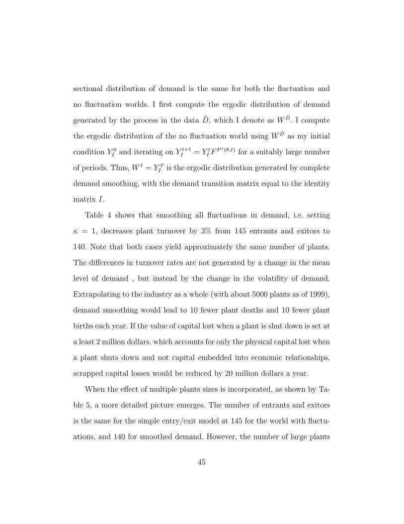
Table 4 shows that smoothing all fluctuations in demand, i.e. setting
κ = 1, decreases plant turnover by 3% from 145 entrants and exitors to
140. Note that both cases yield approximately the same number of plants.
The differences in turnover rates are not generated by a change in the mean
level of demand , but instead by the change in the volatility of demand.
Extrapolating to the industry as a whole (with about 5000 plants as of 1999),
demand smoothing would lead to 10 fewer plant deaths and 10 fewer plant
births each year. If the value of capital lost when a plant is shut down is set at
a least 2 million dollars, which accounts for only the physical capital lost when
a plant shuts down and not capital embedded into economic relationships,
scrapped capital losses would be reduced by 20 million dollars a year.
When the effect of multiple plants sizes is incorporated, as shown by Ta-
ble 5, a more detailed picture emerges. The number of entrants and exitors
is the same for the simple entry/exit model at 145 for the world with fluctu-
ations, and 140 for smoothed demand. However, the number of large plants
45
Data Baseline (κ = 0) Smoothing (κ = 1)
Exitors and Entrants* 142 145 140Number of Plants 2606 2507 2518
*In steady-state, the number of entrants and exitors must be the same.
Table 4: The steady-state number of plants and entrants/exitors under NoDemand Fluctuations and Baseline
increases by 50% from 407 to 598 when demand fluctuations are eliminated.
Thus demand uncertainty appears to leads firms to lower investment in or-
der to reduce their exposure to negative demand shocks. Eliminating demand
fluctuations also reduces the number of plants which switch from small to
big and vice-versa by 6 per year, reducing adjustment costs on the intensive
margin by a small amount.
To identify the contribution of demand fluctuations to plant turnover, de-
mand shocks need to be separated from plant specific shocks to profitability.
These idiosyncratic shocks are potentially large, due to a number of fac-
tors. Perhaps the most thoroughly investigated is the reallocation of output
towards more efficient units (Foster, Haltiwanger, and Syverson, 2005). More-
over, other plant characteristics, such as plant size, being part of a multi-unit
firm, or plant age above 10 years affects the likelihood of exit of plants, as
illustrated by logit regressions on exit reported in Table A11 in section A.
Demand shocks do not account for all the observed plant turnover. 24
24 In Collard-Wexler (2006b), I find that plants experience very large yearly productivityshocks.
46
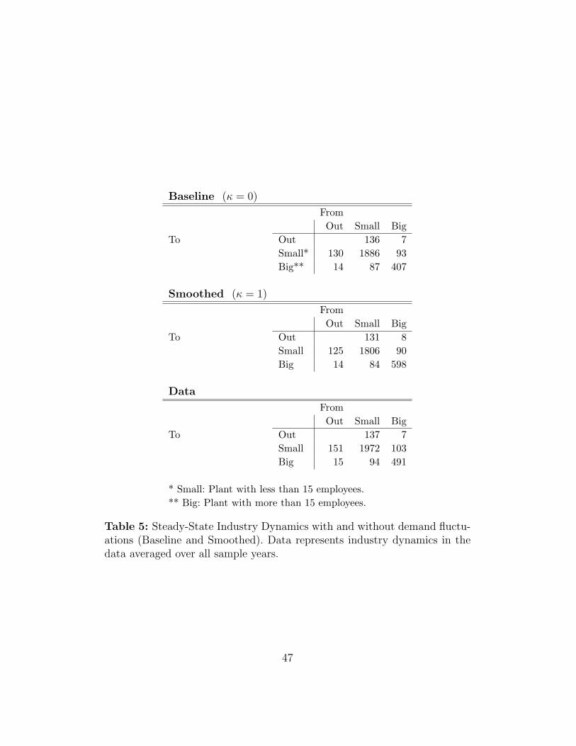
Baseline (κ = 0)
FromOut Small Big
To Out 136 7Small* 130 1886 93Big** 14 87 407
Smoothed (κ = 1)
FromOut Small Big
To Out 131 8Small 125 1806 90Big 14 84 598
Data
FromOut Small Big
To Out 137 7Small 151 1972 103Big 15 94 491
* Small: Plant with less than 15 employees.** Big: Plant with more than 15 employees.
Table 5: Steady-State Industry Dynamics with and without demand fluctu-ations (Baseline and Smoothed). Data represents industry dynamics in thedata averaged over all sample years.
47
7 Conclusion
The Ready-Mix concrete industry is characterized by high sunk costs, due
to capital assets with little resale value and long term relationships with
customers and suppliers. Competition between plants in the same county is
intense, in that a single competitor reduces profits to close to the competi-
tive level. The industry is subject to large demand shocks, on the order of
30% per year. These demand shocks vary across geographically segmented
markets, causing plants to exit declining markets and enter growing ones.
High sunk costs slow the response of entry to demand shocks, allowing firms
to remain in unprofitable markets for some time. High adjustment costs im-
ply that turnover would only be reduced by 3% if demand fluctuations were
eliminated. This policy of demand smoothing would save at most 20 million
dollars a year for this industry from reduced plant exit. Reducing the volatil-
ity of the construction sector is by no means unrealistic, since an important
component of demand is driven by government spending decisions and the
Federal Reserve’s interest rate policy. Yet, demand fluctuations sharply re-
duce firm’s incentives to invest in larger more efficient units, reducing the
number of large plants in the industry by 50%. These larger plants have an
important role in raising the productivity of the industry.
This study focuses on a single industry, which by itself accounts for less
than a tenth of a percent of national output. However, the ready-mix concrete
industry provides a window on potential benefits from reducing uncertainty
48

due to demand fluctuations.
References
Aguirregabiria, V., and P. Mira (2006): “Sequential Estimation of DynamicDiscrete Games,” Econometrica, forthcoming.
Bajari, P., L. Benkard, and J. Levin (2006): “Estimating Dynamic Modelsof Imperfect Competition,” Econometrica, forthcoming.
Bresnahan, T., and P. C. Reiss (1994): “Measuring the Importance of SunkCosts,” Annales d’Economie et de Statistique, 34, 181–217.
Bresnahan, T. F., and P. C. Reiss (1991): “Entry and Competition in Con-centrated Markets,” Journal of Political Economy, 99(5), 33.
Collard-Wexler, A. (2005): “Panel Data Reduces Bias in Entry Models,”Working Paper, New York University.
(2006a): “Appendix for Demand Fluctuations and Plant Turnover in theReady-Mix Concrete Industry,” Working Paper, New York University.
(2006b): “Productivity Dispersion and Plant Selection in the Ready-MixConcrete Industry,” Working Paper, New York University.
Dempster, A. P., N. M. Laird, and D. B. Rubin (1977): “Maximum Like-lihood from Incomplete Data via the EM Algorithm,” Journal of the RoyalStatistical Society. Series B (Methodological), 39(1), 1–38.
Dunne, T., S. D. Klimek, M. J. Roberts, and D. Xu (2006): “Entry andExit in Geographic Markets,” Working Paper, Penn State University.
Dunne, T., M. J. Roberts, and L. Samuelson (1988): “Patterns of Firm En-try and Exit in U.S. Manufacturing Industries,” RAND Journal of Economics,19(4), 495–515.
Ericson, R., and A. Pakes (1995): “Markov-Perfect Industry Dynamics: AFramework for Empirical Work,” The Review of Economic Studies, 62(1), 53–82.
Foster, L., J. C. Haltiwanger, and C. Syverson (2005): “Reallocation,Firm Turnover, and Efficiency: Selection on Productivity or Profitability?,” .
49

Gowrisankaran, G. (1999): “Efficient Representation of State Spaces for SomeDynamic Models,” Journal of Economic Dynamics and Control, 23(8), 1077–1098.
Hotz, V. J., and R. A. Miller (1993): “Conditional Choice Probabilities andthe Estimation of Dynamic Models,” The Review of Economic Studies, 60(3),497–529.
Hotz, V. J., R. A. Miller, S. Sanders, and J. Smith (1994): “A SimulationEstimator for Dynamic Models of Discrete Choice,” The Review of EconomicStudies, 61(2), 265–289.
Jarmin, R. S., and J. Miranda (2002): “The Longitudinal Business Database,”Working Paper, Center for Economic Studies, US Census Bureau.
Kosmatka, S. H., B. Kerkhoff, and W. C. Panarese (2002): Design andcontrol of concrete mixtures, Engineering bulletin ; 001. Portland Cement Asso-ciation, Skokie, Ill., 14th edn.
Lucas Jr, R. E. (1978): “On the Size Distribution of Business Firms,” The BellJournal of Economics, 9(2), 508–523.
Maskin, E., and J. Tirole (1988): “A Theory of Dynamic Oligopoly, I: Overviewand Quantity Competition with Large Fixed Costs,” Econometrica, 56(3), 549–569.
McBride, M. E. (1983): “Spatial Competition and Vertical Integration: Cementand Concrete Revisited,” American Economic Review, 73(5), 1011–22.
Pakes, A., S. Berry, and M. Ostrovsky (2006): “Simple estimators for the pa-rameters of discrete dynamic games, with entry/exit examples,,” RAND Journalof Economics, forthcoming.
Pakes, A., and P. McGuire (1994): “Computing Markov-Perfect Nash Equilib-ria: Numerical Implications of a Dynamic Differentiated Product Model,” TheRand Journal of Economics, 25(4), 555–589.
(2001): “Stochastic Algorithms, Symmetric Markov Perfect Equilibrium,and the ’Curse’ of Dimensionality,” Econometrica, 69(5), 1261–1281.
Pesendorfer, M., and P. Schmidt-Dengler (2003): “Identification and Es-timation of Dynamic Games,” NBER Working Paper 9726,.
50

Ramey, V. A., and M. D. Shapiro (2001): “Displaced Capital: A Study ofAerospace Plant Closings,” Journal of Political Economy, 109(5), 958–992.
Rust, J. (1987): “Optimal Replacement of GMC Bus Engines: An EmpiricalModel of Harold Zurcher,” Econometrica, 55(5), 999–1033.
Ryan, S. P. (2006): “The Costs of Environmental Regulation in a ConcentratedIndustry,” Working Paper, M.I.T.
Syverson, C. (2004): “Market Structure and Productivity: A Concrete Exam-ple,” Journal of Political Economy, 112(6), 1181–1222.
51

A Tables and Figures
Sector Name NAICS Concrete sector as fraction ofTotal Sales Materials Used
Owner-occupied dwellings S00800 21% NANew residential 1-unit structures 230110 17% 3%New residential additions and alterations 230130 10% 7%Commercial and institutional buildings 230220 9% 2%Highway, street, bridge, and tunnel construction 230230 8% 7%New multifamily housing structures 230120 7% 10%Other new construction 230250 4% 2%Maintenance and repair of nonresidential buildings 230320 3% 2%Real Estate 31000 3% NAMaintenance and repair of residential structures 230310 2% 3%Other State and local government enterprises. S00203 2% NAPower generation and supply 221100 2% NAManufacturing and industrial buildings 230210 1% 2%New farm housing units 230140 1% 7%Other maintenance and repair construction 230340 1% 2%Water, sewer, and pipeline construction 230240 1% 1%Maintenance and repair of highways, streets 230330 0.4% 1%Total For selected Sectors 92%
Table A1: Concrete purchases by sector, and relative importance of concretecosts for the sector.
Source: 1997 Benchmark Input-Output Tables.
52

Number of Concrete Plants Number of Counties/Years Percent
0 22,502 30%1 23,276 31%2 12,688 17%3 6,373 9%4 3,256 4%5 1,966 3%6 1,172 2%More than 6 3,205 4%Total 74,438
Table A2: Most counties in the United States are served by less than 6ready-mix concrete plants.
Product Fraction of output in value
Ready-Mix Concrete 95%Unknown 4%Construction sand and gravel 2%Precast Concrete Products 1%Asphalt Paving Mixtures and Blocks 1%
Table A3: Plants in sample tend to produce concrete exclusively
53

Year Birth Continuer Death
1976 501 4,737 N.A.1977 557 4,791 4101978 327 5,043 4451979 392 5,093 3331980 271 5,140 3871981 313 5,069 3601982 313 4,875 4231983 273 4,991 3151984 328 4,972 2951985 309 4,988 3391986 300 5,003 3051987 390 4,898 4041988 270 5,016 2691989 248 4,275 4481990 194 4,103 3041991 220 3,882 2911992 214 4,643 3481993 133 3,668 2701994 163 3,952 2321995 196 3,840 2431996 195 3,734 2301997 338 4,768 2741998 239 4,949 2671999 320 4,961 234
Table A4: The number of Births, Deaths and Continuers is fairly stableover the last 25 years
54

Obs
erva
tion
sM
ean
Stan
dard
5th
95th
Dev
iati
onPer
cent
ilePer
cent
ile
Frac
tion
inLB
Dco
ncre
tesi
c18
7825
0.78
0.33
01
Frac
tion
inA
sm/C
mfco
ncre
tein
d18
7915
0.92
0.22
0.33
1Tot
alV
alue
ofSh
ipm
ents
(in
000’
s)70
566
3380
2564
341
1100
0Tot
alE
mpl
oym
ent
7056
626
147
182
Adm
inis
trat
ive
Rec
ord
Fla
g70
622
0.13
0.34
01
Bui
ldin
gA
sset
sE
ndin
g(i
n00
0’s)
5124
615
318
850
420
Cos
tof
Fuel
s(i
n00
0’s)
7056
642
245
015
0C
ost
ofR
esal
es(i
n00
0’s)
7056
611
516
210
430
Cos
tof
Con
trac
tW
ork
(in
000’
s)70
566
2223
50
37C
ost
ofP
urch
ased
Ele
ctri
city
(in
000’
s)70
566
2923
60
75Tot
alV
alue
ofIn
vent
ory
(in
000’
s)11
598
116
3702
014
0M
achi
nery
Ass
ets
End
ing
(in
000’
s)51
246
754
4463
027
00M
achi
nery
Dep
reci
atio
n(i
n00
0’s)
5124
655
478
022
0M
ater
ials
Inve
ntor
yE
ndin
g(i
n00
0’s)
7056
615
172
040
250
Mac
hine
ryR
ents
(in
000’
s)57
073
1295
042
Mac
hine
ryR
etir
emen
ts(i
n00
0’s)
5124
624
238
078
Mul
ti-U
nit
Fla
g,M
U=
labe
l70
622
0.51
0.50
01
Tot
alN
ewE
xpen
ditu
res
(in
000’
s)70
566
148
1625
051
0N
ewM
achi
nery
Exp
endi
ture
s(i
n00
0’s)
7056
612
813
510
460
Table
A5:
Sum
mar
ySta
tist
ics
for
Pla
nt
Dat
a
55

Obs
erva
tion
sM
ean
Stan
dard
5th
95th
Dev
iati
onPer
cent
ilePer
cent
ile
Cou
nty
Tot
alV
alue
ofSh
ipm
ent
(in
000’
s)24
677
3181
1201
00
1400
0C
ount
yV
alue
Add
ed(i
n00
0’s)
2467
714
0852
890
6500
Cou
nty
Tot
alA
sset
sE
ndin
g(i
n00
0’s)
2467
710
9014
134
047
00C
ount
yTot
alE
mpl
oyem
ent
2467
722
690
100
Cou
nty
Tot
alSa
lari
esan
dW
ages
(in
000’
s)24
677
559
2018
026
00C
ount
yC
oncr
ete
Pla
nts
7443
51.
863.
240
6C
ount
yE
mpl
oym
ent
7443
527
.24
79.0
30
110
Cou
nty
Pay
roll
(in
000’
s)74
435
4238
7439
60
3600
Cou
nty
Pla
ntB
irth
s74
435
0.11
0.42
01
Cou
nty
Pla
ntD
eath
s74
435
0.10
0.37
01
Cou
nty
0-5
Em
ploy
eeP
lant
s74
435
0.52
1.07
02
Cou
nty
5-20
Em
ploy
eeP
lant
s74
435
0.78
1.34
03
Cou
nty
mor
eth
an20
Em
ploy
eeP
lant
s74
435
0.86
1.49
03
Cou
nty
Pla
nts
Les
sth
an5
year
sol
d74
435
0.17
0.76
01
Cou
nty
Pla
nts
5-10
Yea
rsO
ld74
435
0.54
1.47
02
Cou
nty
Pla
nts
over
10Y
ears
Old
7443
51.
352.
070
4C
ount
yA
rea
7226
911
4738
9121
032
00E
mpl
oym
ent
inC
onst
ruct
ion
6991
114
9553
9011
6800
Pay
roll
inC
onst
ruct
ion
(in
000’
s)69
911
3713
516
3546
110
1600
00
Table
A6:
Sum
mar
ySta
tsfo
rC
ounty
Agg
rega
teD
ata
56
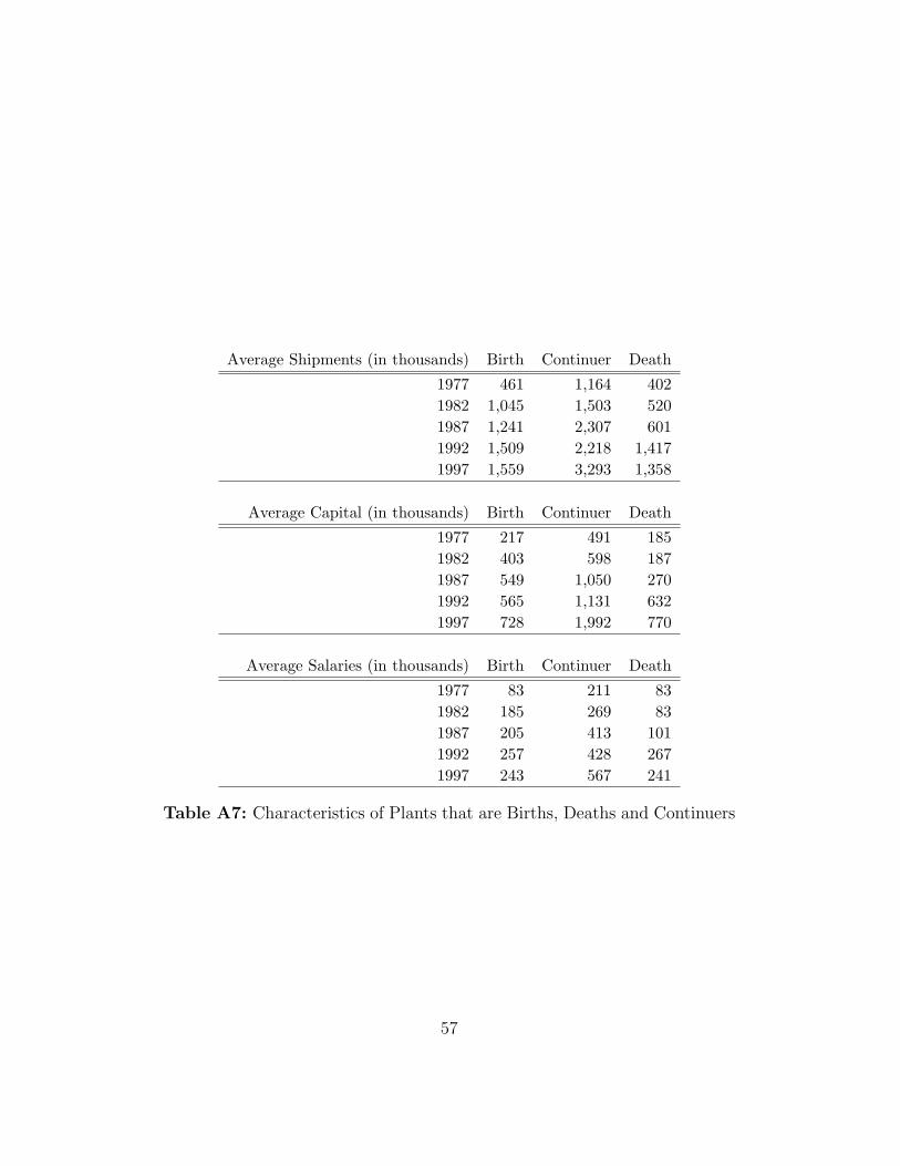
Average Shipments (in thousands) Birth Continuer Death
1977 461 1,164 4021982 1,045 1,503 5201987 1,241 2,307 6011992 1,509 2,218 1,4171997 1,559 3,293 1,358
Average Capital (in thousands) Birth Continuer Death
1977 217 491 1851982 403 598 1871987 549 1,050 2701992 565 1,131 6321997 728 1,992 770
Average Salaries (in thousands) Birth Continuer Death
1977 83 211 831982 185 269 831987 205 413 1011992 257 428 2671997 243 567 241
Table A7: Characteristics of Plants that are Births, Deaths and Continuers
57

3%
4%
5%
6%
7%
8%
9%
10%
11%
12%
1977
1978
1979
1980
1981
1982
1983
1984
1985
1986
1987
1988
1989
1990
1991
1992
1993
1994
1995
1996
1997
1998
1999
Year
Entr
y/Ex
it R
ate
Entry RateExit Rate
Figure A1: Net Entry is sensitive to the business cycle.
Price per Cubic Yard in 1963 Dollars Coefficient S.E.
1 Competitor -0.95 (0.21)2 Competitors -1.19 (0.21)3 Competitors -1.38 (0.24)4 Competitors -1.33 (0.24)5 Competitors -1.57 (0.25)6 Competitors -1.69 (0.27)7 Competitors -1.72 (0.30)8 Competitors -1.78 (0.31)Area in thousand of acres 0.28 (0.04)Year Effects(Base Year 1963) YesConstant about 42
Number of Observations 3148Sum of Deviations 18225Pseudo-R2 17%
Table A8: Median Regression of Prices pooled over the entire sample onthe Number of Plants in a county
58

Price and Competition
40
40.5
41
41.5
42
0 1 2 3 4 5 6 7 8
Number of Competitors
Med
ian
Pric
e of
a c
ubic
yar
d of
con
cret
e in
19
63 d
olla
rs
Figure A2: Prices Decline Dramatically with the addition of the first com-petitors, and little afterwards.Note: Bars represent 95% confidence interval on median price. I report thecomplete median regression in Table A8 in section A.25
Next Year’s Construction Employement OLS S.E. Fixed Effect S.E.
construction employement t 0.657 (0.008) 0.506 (0.009)construction employement t-1 0.216 (0.008) 0.129 (0.008)construction employement t-5 0.114 (0.005) -0.010 (0.007)interest rate -0.012 (0.001) -0.027 (0.001)interate rate*payroll 0.000 (0.000) 0.000 (0.000)constant 0.218 (0.013) N.A.
Number of Group 14333 1339Number of Time Periods N.A. 11R2 97% 96%R2-within N.A. 49%F-statistic 98075 2585
Table A9: Forecasting the Evolution of Demand for Concrete with OLS andcounty fixed effect regressions
59

Net Present Value in Thousands of Dollars
Log Construction Workers 2171 Competitor -1,4932 Competitor -1713 Competitor -1984 and More Competitor -80Sunk Cost 1,242Fixed Cost -499
Normalized By Decrease in Price in % from monopolyto duopoly times average sales
Table A10: Dollar Value of Sunk Costs from the model match InterviewData
Plant Size and Exit
0%
2%
4%
6%
8%
10%
12%
14%
16%
1 2 3 4 5 6 7 8 9 10
Decile of Employement
Exit
Prob
abili
ty
Figure A3: Small firms are much more likely to exit than large firms
60

Baseline Exit probability 4.51%Parameter Standard Error
Employees -0.11% (0.02%)Employees*Employement Construction 0.01% (0.00%)5-10 Years Old 0.74% (0.15%)0-5 Years Old 0.30% (0.17%)Multi-Unit Firm -1.82% (0.11%)Less than 6 employees 4.98% (0.22%)Log of county construction employment -0.24% (0.19%)Log of county concrete plants 1.49% (0.18%)Square log of construction employement -0.22% (0.05%)Square log of concrete plants 0.00% (0.01%)
Number of Observations 143204Log-Likelihood -28396Pseudo-R2 4.7%
Table A11: Marginal Effects on the Probability of Exit estimated from aLogit
61
Recommended