62
CHAPTER 4
DESIGN OF LEAF IMAGE ENHANCEMENT METHOD
A major factor that influences the quality of leaf image data is noise. The
presence of noise often reduces the amount of information that can be gained from the
image and sometimes obscures important image regions. According to
www.wikipedia.org, image noise is defined as the random variation of brightness or
color information in images produced during acquisition. Noise in leaf image is the
consequence of various types of errors caused due to various factors like environment
and equipment used and is introduced due to errors occurring during acquisition,
transmission, compression and storage of images. It is considered as an undesirable
by-product that is introduced into the image by any one of the following scenarios.
• Scanner : When a leaf photograph made on film is scanned, noise may be
introduced as the result of damage to the film or by the scanner itself and is
generally shown as grains in the image.
• Digital Equipment : If the leaf image is captured directly in digital format (for
example using a CCD camera), noise is introduced by the equipment itself.
• Transmission : The leaf image is also degraded by noise acquired during
transmission
• Storage : The method used for compression that makes efficient use of storage
resources also introduces noise and artifacts into the leaf image.
Regardless of the source of noise, they are generally regarded as an undesirable
by-product. Identifying and quantifying these factors is a difficult and challenging
task. Due to these challenges, the field is still an active research area and generally
integrates sophisticated image processing techniques with Human Visual System
(HVS).

63
This chapter presents the methods and techniques which is used to remove
noise from the leaf images. The main goal here is to enhance the leaf image in a
manner that increases the visual quality of the leaf image so as to increase the
efficiency of CAP-LR system. The design and development of a noise removal
algorithm that meets the above goal is vital, as imprecise filtering might degrade the
performance of leaf segmentation, feature detection and feature extraction which have
a direct impact on plant recognition end result. Leaf images are normally degraded by
the presence of Gaussian noise which causes low or high contrast, occurring both in
the edge area and the image area. In general, preprocessing an image includes the
removal of noise, edge or boundary enhancement, automatic contrast adjustment and
segmentation. In this chapter, an approach that simultaneously removes noise, adjusts
contrast and enhances boundaries is presented. The proposed desnoising algorithm is
termed as ‘Enhanced Wavelet based Denoising with inbuilt Edge Enhancement and
Automatic Contrast Adjustment Algorithm (WEC Method)’.
4.1. BASIC CONCEPTS
As mentioned previously, leaf images are widely used by botanists and
researchers interested in plant life to identify and recognize plants to which it belongs.
Contrast adjustment, noise removal and edge enhancement are operations that are
mandatory in pre-processing steps for the successful design of CAP-LR system. The
Proposed WEC algorithm proposes to enhance the leaf image using a novel
amalgamation of the existing algorithms to increase the quality of the image. It
performs three operations namely
Contrast adjustment
Noise removal
Edge Enhancement
4.1.1. Contrast Enhancement
Contrast generally refers to the difference in luminance or grey level values in
an image and is an important characteristic during image enhancement. It can be
defined as the ratio of the maximum intensity to the minimum intensity over an image
64
and this ratio has a strong bearing on the detectability and resolving power of an
image. Larger this ratio, the more easy it is to interpret the image. Leaf images used to
identify a plant, generally, lack adequate contrast and, hence, require contrast
improvement.
Contrast enhancement technique expands the range of brightness values in an
image so that the image can be efficiently displayed in a manner desired. The density
values in an image are expanded over a greater range. The effect of contrast
enhancement increases visual contrast between two areas having different uniform
densities. The resultant image enables the researcher or analysts to differentiate easily
between areas initially having a small difference in density.
4.1.2. Noise Removal
Leaf images are generally degraded by Gaussian noise, where each pixel in the
leaf image is changed from its original value by a (usually) small amount. A
histogram is defined as a plot that exhibits the amount of distortion of a pixel value
against the frequency with which it occurs, shows a normal distribution of noise. This
type of noise is a major part of the “read noise” of an image sensor, that is, of
the constant noise level in dark areas of the image (Nakamura, 2005;
http://en.wikipedis.org/wiki/Image_noise-cite_note-3). The standard model of
amplifier noise is additive Gaussian, dependent at each pixel and dependent on the
signal intensity which is primarily caused by thermal noise (Johnson–Nyquist noise),
including the reset noise, also called as ‘kTC noise’, which comes from the capacitors.
It is in the form of white noise and is caused by the random fluctuations in the signal
(Ohta, 2008). In color cameras where more amplification is used in the blue color
channel than in the green or red channels, there can be more noise in the blue channel.
Amplifier noise is a major part of the noise appearing on an image sensor, that is, of
the constant noise level in dark areas of the image.
Gaussian noise is statistical noise that has its probability density function equal
to that of the normal distribution or Gaussian distribution [1]. While other
distributions are possible, the Gaussian (normal) distribution is usually a good model,

65
due to the central limit theorem that states that the sum of different noises tends to
approach a Gaussian distribution.
Some examples of leaf images that are affected by Gaussian noise are shown in
Figure 4.1.
Original Degraded Original Degraded
Original Degraded Original Degraded
Figure 4.1 : Original and Gaussian Noise Degraded Images
4.1.3. Edge Enhancement
An edge in an image represents the objects of an image in a higher level of
abstraction and forms the most fundamental primitive image characteristics. Edges are
also one of the most important components of Human Visual System and are
generally considered as color independent features used during object recognition and
detection. Physcophysical experiments indicate that an image with accentuated or
crispened edges often provides more information than the original image. The purpose
of edge enhancement is to highlight the fine details in an image or to restore details
that have been blurred due to errors that occur during image acquisition. Edge
enhancement technqiues sharpen the outlines of objects and features in an image with
respect to their background.

66
Edge enhancement is an image processing filter that works by identifying sharp
edge boundaries in the image, such as the edge between a background and a subject
having contrasting color. After finding such an edge boundary, the contrast in that
area is increased around the edge. This result in creating subtle bright and dark
highlights on either side of any edges in the image, making the edge more defined.
The result of edge enhancement depends on different number of properties and
some significant properties among them are listed below.
Amount. This property controls the extent to which contrast in the edge
detected area is enhanced.
Radius or aperture. This property affects the size of the edges (to be detected
or enhanced) and the area (surrounding the edge that will be altered by the
enhancement). A small radius value results in enhancement applied only to
sharper and finer edges and thus is confined to a smaller area around the edge.
Threshold. This mechanism adjusts the sensitivity of the edge detection
whenever required. A lower threshold results in more subtle boundaries of
color being identified as edges. A threshold that is too low may result in some
small parts of surface textures, noise or film grain being incorrectly identified
as being an edge.
Unlike some forms of image sharpening, edge enhancement does not enhance
subtle details that may appear in more uniform areas of the image, such as texture or
grain, which appears in flat or smooth areas of the image. The advantage obtained is
that the imperfections in the image reproduction, such as noise, or imperfections in the
subject, such as natural imperfections, are not made more obvious by the process. An
disadvantage to this is that the image may begin to look less natural, as the sharpness
of the overall image increases the level of detail flat, smooth areas does not. As with
the other forms of edge enhancement and image sharpening is only capable of
improving the perceived sharpness of an image. The operation of enhancement is not
67
completely reversible and as such some detail in the image is lost as a result of
filtering and has to be designed in a careful manner.
4.2. MOTIVATION
Most of the traditional edge enhancement filters that performs enhancement
operations that consider the whole image as a single unit, and use enhancement
operations to regions whose gray values vary largely. Because of the presence of noise
in leaf images, these types of edge enhancers might enhance the noise and degrade the
contrast of the original image. Moreover, traditional algorithms cannot differentiate a
reverberation artifact that appears like an edge and accidently enhances them also thus
further reduce the quality of the image.
Contrast enhancement is usually achieved by histogram equalization in the
spatial domain to redistribute gray levels uniformly. Existing techniques, however,
while adjusting gray levels, lose some important information. Meanwhile, edge
enhancement attempts to emphasize the fine details in the original image. But in
spatial domain, it is hard to selectively enhance details at different scales. Further, in
the spatial domain, applying operations for adjusting contrast and enhancing the edges
in different orders may yield different enhancement results.
Wavelet-based image analysis provides multiple representations of a single
image. It decomposes an image into approximated-coefficients and multi-resolution
detailed-coefficients. To overcome the above spatial domain enhancement issues, this
study proposes a wavelet-based image enhancement method combined with a noise
removal procedure is proposed. Since the various enhancement procedures are applied
on different components in the wavelet domain, they work independently and do not
affect each other. Moreover, the order of applying both of them becomes irrelevant. A
detailed description of the algorithm is presented in the following section.
4.3. THE WEC METHOD
The proposed desnoising algorithm is termed as ‘Enhanced Wavelet based
Denoising with inbuilt Edge Enhancement and Automatic Contrast Adjustment

68
Algorithm (WEC Method)’. The method combines the use of CLAHE (Contrast
Limited Adaptive Histogram Equalization) algorithm with Discrete Wavelet co-
efficients for enhancing the contrast of the input leaf image. The Discrete Wavelet
Transform (DWT) was used to obtain the edge and non-edge information of the
image. Edge enhancement was performed using a sigmoid function and for noise
removal a relaxed median filter was used. The various steps involved are shown in
Figure 4.2 and are described in the following sections.
4.3.1 Step 1 : Color Space Transformation
A color model is an abstract mathematical model describing the way colors can
be represented as tuples of numbers, typically as three or four color components (e.g.
RGB and CMYK are color models) and the mapping of colors from the color model is
the color space(Wyszeeki,1982). The two most widely used color spaces for storing
digital images are RGB color space and YUV color space. The RGB color space is
defined by the three chromaticities of the red, green, and blue additive primaries, and
can produce any chromaticity that is the triangle defined by those primary colors.
RGB stores a color value for each of the color levels, Red, Green and Blue. That is, it
uses 8 bits to each color level (thus the range 0-255 obtained from 28), thus using 24
bits to store color information.

69
Figure 4.2 : Steps in WEC Method
YUV colorspace works on the principle that, as human eye perceives changes
in brightness rather than changes in color and focuses more on brightness than the
actual brightness level. There are three values while using YUV color space
(http://en.wikipedia.org/wiki/YUV). They are,
Luminance (Luma, which is the brightness level) is abbreviated as Y.
U is the red difference sample
V is the blue difference sample
YUV color space is stored using 16 bits, where 8 bits are used by Luma and 4 bits are
used by U and V. Thus, YUV stores more relevant data at a lower accuracy than RGB.
Moreover, it is well known that the RGB components of color images are highly
correlated and if the wavelet transforms of each color component is obtained, the
transformed components will also be highly correlated (Nobuhara and Hirota, 2004).
Therefore, a color transformation that reduces the redundancy and correlation of the
image is highly desired. Many linear transformations can be used such as the YUV,
KLT, YCrCb or L*a*b*. This study uses a YUV color transformation for the
following reasons:
Leaf Image
Discrete Wavelet Transformation
Edge Coefficient Detailed Coefficient
Contrast Adjustment (CLAHE)
Boundary Enhancement(Sigmoid Function)
Median FilterDenoising
Inverse Discrete Wavelet Transformation
Enhanced Leaf image

70
(i) The YUV color model represents the human perception of color more
closely than the standard RGB model used in computer graphics
hardware, and ,
(ii) The YUV color model stores more relevant data at a lower accuracy
than RGB.
The equation used for converting or transforming the RGB components to YUV space
is given in Equation (5.2).
B
G
R
100.0515.0615.0
437.0289.0418.0
114.0587.0200.0
V
U
Y
(5.2)
4.3.2. Step 2 : Wavelet Transformation
The purpose of this step is to apply Haar wavelet decomposition algorithm on a
given image to obtain its wavelet coefficients. The given image is decomposed into
several components in multi-resolution space by applying a forward wavelet
transform. Different wavelet filter sets and/or different number of transform-levels
results in different decomposition results. While any wavelet-filters can be used with
the proposed scheme, the discussion is based on Haar wavelet. The application of
Haar wavelet transform resulted in four subbands namely, LL (approximation
coefficients) and HL, LH and HH (detailed coefficients).
4.3.3. Step 3 : Automatic Contrast Adjustment
The first step of WEC method is to adjust the contrast of the input leaf image
automatically using CLAHE algorithm. CLAHE is a form of high-pass filtering where
low-frequency information (large-scale intensity variation) is blocked and thus can
improve the contrast and sharpen edges of an image simultaneously.
CLAHE (Wanga et al., 2004) is a special case of the histogram equalization
technique (Gonzalez and Woods, 2007), which seeks to reduce the noise and edge-

71
shadowing effect produced in homogeneous areas. CLAHE is a technique used to
improve the local contrast of an image. This method is a generalization of adaptive
histogram equalization and ordinary histogram equalization. The algorithm partitioned
the images into contextual regions and applied the histogram equalization to each one.
This evens out the distribution of grey values and makes the hidden features of the
image more visible. The full grey spectrum was used to express the image. CLAHE is
an improved version of AHE, or Adaptive Histogram Equalization, to overcome the
limitations of standard histogram equalization. This section describes the working of
CLAHE algorithm.
The traditional histogram equalization algorithm is a method used for adjusting
contrast using the image's histogram. This algorithm works efficiently for smaller
images or images where almost all of the different intensity levels are represented. Hit
is a technique for recovering lost contrast in an image by remapping the brightness
values, so that the brightness values are equalized or more evenly distributed. As a
side effect, the histogram of its brightness values becomes flatter. The traditional
histogram equalization algorithm is shown in below.
1. Read the input leaf image
2. Convert image to gray scale
3. Construct the histogram of the image (H[x]). This is a 256 value array
containing the number of pixels with value x
4. Calculate the cumulative density function of the histogram (cdf[x]). This is a
256 value array containing the number of pixels with value x or less, that is,
cdf[x] = H[0] + H[1] + H[2] + ... + H[x]
5. Loop through the n pixels in the entire image and replace the value at each ith
point by V[i], which is calculated as floor(255*(cdf[V[i]] - cdf[0])/(n - cdf[0]))
The result of step 5 is the contrast adjusted image. However, the major
drawback of histogram equalization algorithm is the introduction of blocking artifacts
introduced. This can be solved by using an Adaptive Histogram Equalization (AHE)
algorithm. The pseudo code for adaptive histogram equalization algorithm is given in
Figure 4.3 (Zhiming and Jianhua, 2006).
72
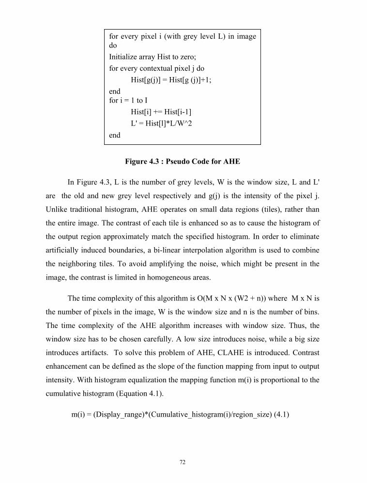
Figure 4.3 : Pseudo Code for AHE
In Figure 4.3, L is the number of grey levels, W is the window size, L and L'
are the old and new grey level respectively and g(j) is the intensity of the pixel j.
Unlike traditional histogram, AHE operates on small data regions (tiles), rather than
the entire image. The contrast of each tile is enhanced so as to cause the histogram of
the output region approximately match the specified histogram. In order to eliminate
artificially induced boundaries, a bi-linear interpolation algorithm is used to combine
the neighboring tiles. To avoid amplifying the noise, which might be present in the
image, the contrast is limited in homogeneous areas.
The time complexity of this algorithm is O(M x N x (W2 + n)) where M x N is
the number of pixels in the image, W is the window size and n is the number of bins.
The time complexity of the AHE algorithm increases with window size. Thus, the
window size has to be chosen carefully. A low size introduces noise, while a big size
introduces artifacts. To solve this problem of AHE, CLAHE is introduced. Contrast
enhancement can be defined as the slope of the function mapping from input to output
intensity. With histogram equalization the mapping function m(i) is proportional to the
cumulative histogram (Equation 4.1).
m(i) = (Display_range)*(Cumulative_histogram(i)/region_size) (4.1)
for every pixel i (with grey level L) in imagedoInitialize array Hist to zero;for every contextual pixel j do
Hist[g(j)] = Hist[g (j)]+1;endfor i = 1 to I
Hist[i] += Hist[i-1]L' = Hist[l]*L/W^2
end
73
Thus, the derivative of m(i) is proportional to histogram(i). So, the important
task of CLAHE is to limit the histogram, which, in turn, limits the contrast
enhancement. The algorithm is given in Figure 4.4 (Garg et al., 2011). In the
experiments, NB was set to 64, CL was set to 0.01 and tile size used was 8 x 8 and the
histogram distribution was Bell-Shaped.
4.3.4. Step 4 : Edge Enhancement
Edge enhancement is one of the most fundamental operations in image
analysis. Edges are considered as the outline of an object or as the boundary between
an object and the background. An edge in an image is normally defined as the
transition in the intensity of that image. If the edges in an image can be identified
precisely, all objects can be located and basic properties such as area, shape and
perimeter can be measured efficiently.

74
Figure 4.4 : CLAHE Algorithm
Edge detection, in general, consists of two parts:
edge enhancement - Process of calculating the edge magnitude at each
pixel
edge localization - Process of determining the exact location of the edge.
Once an edge is enhanced properly, the location of the edge can be identified
accurately. Thus, the performance of edge detection depends on the enhancement of
edges. Edge enhancement improves the quality of edges so as to help in the
segmentation and recognition steps of CAP-LR system. Edge enhancement filters
enhance the local discontinuities at the boundaries of different objects (edges) in the
image. Fixed size edge operators, like the gradient operations, always enhance both
Input : Leaf Image, No. of bins (NB) of the histograms used in buildingimage transform function (dynamic range), No. of regions in row andcolumn directions, Clip Limit (CL) for constrast limiting (normalized from 0to 1)
Output : Contrast Adjusted Image
1. Divide input image into 'n' number of non-overlapping contextualregions (tile) of equal sizes (8 x 8 used in experiments).
2. Process each contextual region (tile) thus producing gray levelmappings, extract a single image region and perform the following:
a. Construct a histogram for each region using NB
b. Clip the histogram such that its height does not exceed CL(Histogram Redistribution).
c. Create a mapping (transformation function) for this region usingEquation 4.1.
d. Interpolate gray level mappings in order to assemble finalCLAHE image: Extract cluster of four neighbouring mappingfunctions, process image region partly overlapping each of themapping tiles, extract a single pixel, apply four mappings to thatpixel, and interpolate between the results to obtain the outputpixel
75
strong reflectors and speckle noise, spread the detected edges and decrease the
contrast resolution of the image. Edge enhancement involves sharpening the outlines
of objects and features with respect to their background.
This section is dedicated to enhance the edges of leaf images so as to improve
the detectability of the leaf’s borders. The main aim is to find edge structures and
enhance weak borders of the leaf image. Most of the reported works have
concentrated on edge detection (Bao et al., 2005; Yu and Acton,2004) but report that
have focused on edge enhancement of leaf images are sparse.
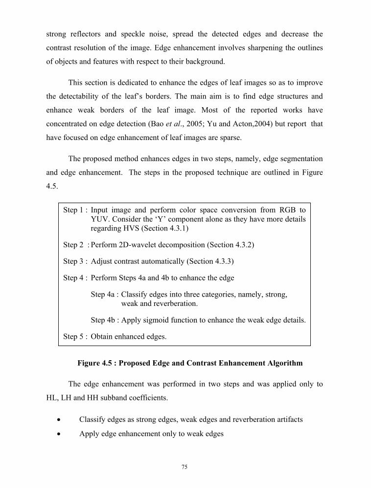
The proposed method enhances edges in two steps, namely, edge segmentation
and edge enhancement. The steps in the proposed technique are outlined in Figure
4.5.
Figure 4.5 : Proposed Edge and Contrast Enhancement Algorithm
The edge enhancement was performed in two steps and was applied only to
HL, LH and HH subband coefficients.
Classify edges as strong edges, weak edges and reverberation artifacts
Apply edge enhancement only to weak edges
Step 1 : Input image and perform color space conversion from RGB toYUV. Consider the ‘Y’ component alone as they have more detailsregarding HVS (Section 4.3.1)
Step 2 : Perform 2D-wavelet decomposition (Section 4.3.2)
Step 3 : Adjust contrast automatically (Section 4.3.3)
Step 4 : Perform Steps 4a and 4b to enhance the edge
Step 4a : Classify edges into three categories, namely, strong,weak and reverberation.
Step 4b : Apply sigmoid function to enhance the weak edge details.
Step 5 : Obtain enhanced edges.
76
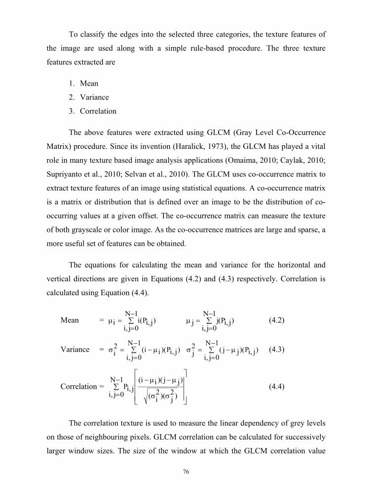
To classify the edges into the selected three categories, the texture features of
the image are used along with a simple rule-based procedure. The three texture
features extracted are
1. Mean
2. Variance
3. Correlation
The above features were extracted using GLCM (Gray Level Co-Occurrence
Matrix) procedure. Since its invention (Haralick, 1973), the GLCM has played a vital
role in many texture based image analysis applications (Omaima, 2010; Caylak, 2010;
Supriyanto et al., 2010; Selvan et al., 2010). The GLCM uses co-occurrence matrix to
extract texture features of an image using statistical equations. A co-occurrence matrix
is a matrix or distribution that is defined over an image to be the distribution of co-
occurring values at a given offset. The co-occurrence matrix can measure the texture
of both grayscale or color image. As the co-occurrence matrices are large and sparse, a
more useful set of features can be obtained.
The equations for calculating the mean and variance for the horizontal and
vertical directions are given in Equations (4.2) and (4.3) respectively. Correlation is
calculated using Equation (4.4).
Mean = )j,iP(i1N
0j,ii
)j,iP(j
1N
0j,ij
(4.2)
Variance = )j,iP)(ii(1N
0j,i2i
)j,iP)(jj(
1N
0j,i2j
(4.3)
Correlation =
)2j)(2
i(
)jj)(ii(j,iP
1N
0j,i(4.4)
The correlation texture is used to measure the linear dependency of grey levels
on those of neighbouring pixels. GLCM correlation can be calculated for successively
larger window sizes. The size of the window at which the GLCM correlation value

77
declines suddenly may be taken as one definition of the size of definable objects
within an image. GLCM correlation is independent of mean and variance features and
has a more intuitive meaning to the actual calculated values, that is, a 0 represents
uncorrelated, 1 represents perfectly correlated features. The texture features thus
extracted were quantized using the following simple procedure.
Let t1, … tn be the set of feature values extracted for a particular feature.
Initially, the maximum (Max), minimum (Min) and mean () of this set is calculated,
from which the size of quantization interval at left (QL) and right (QR) of the mean
value obtained were estimated using Equation (4.5) with a total quantization level as
6.
6)Min(2
LQ
6
)Max(2QR
(4.5)
Using QL and QR, the ratio of quantization level can be calculated as
K = QL/QR (4.6)
and the quantization Qi of value ti can be calculated as follows.
R = (ti – Min)/QR
If R < ½, then Qi = R else Qi = ((R-1/2)/K) + (l/2) (l=6)
Calculate QL and QR for the quantized values and group them into four ranges,
namely, Large, Medium, Small and Very Small. Small values were from 0 to QL,
medium values were from QL to QR and large values were all values greater than QR.
All values which are less than 0 were considered very small.
Using the above quantized texture features the edges were classified as strong,
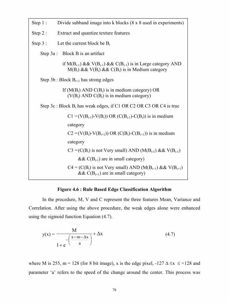
weak and artifact using a rule-based procedure (Figure 4.6).
78
Figure 4.6 : Rule Based Edge Classification Algorithm
In the procedure, M, V and C represent the three features Mean, Variance and
Correlation. After using the above procedure, the weak edges alone were enhanced
using the sigmoid function Equation (4.7).
y(x) = xΔ
e1
M
axΔmx
(4.7)
where M is 255, m = 128 (for 8 bit image), x is the edge pixel, -127 x +128 and
parameter ‘a’ refers to the speed of the change around the center. This process was
Step 1 : Divide subband image into k blocks (8 x 8 used in experiments)
Step 2 : Extract and quantize texture features
Step 3 : Let the current block be Bi
Step 3a : Block B is an artifact
if M(Bi-1) && V(Bi-1) && C(Bi-1) is in Large category ANDM(Bi) && V(Bi) && C(Bi) is in Medium category
Step 3b : Block Bi+1 has strong edges
If (M(Bi) AND C(Bi) is in medium category) OR(V(Bi) AND C(Bi) is in medium category)
Step 3c : Block Bi has weak edges, if C1 OR C2 OR C3 OR C4 is true
C1 =(V(Bi-1)-V(Bi)) OR (C(Bi-1)-C(Bi)) is in medium
category
C2 =(V(Bi)-V(Bi+1)) OR (C(Bi)-C(Bi+1)) is in medium
category
C3 =(C(Bi) is not Very small) AND (M(Bi-1) && V(Bi-1)
&& C(Bi-1) are in small category)
C4 = (C(Bi) is not Very small) AND (M(Bi+1) && V(Bi+1)&& C(Bi+1) are in small category)
79
repeated for all detailed coefficients. The above procedure identified all high intensity,
large variance and high correlation coefficients as strong edges and all coefficients
with significant changes in variance and correlation as weak edges.
4.3.5. Step 5 : Noise Removal
The next step is to remove the noise from detailed coefficients. For this
purpose, a relaxed median filter was used. Traditional median filter uses a window
that slides across the image data and the median value inside the window is taken as
the output value. The filter is efficient in noise removal. However, the filter sometimes
removes sharp corners and thin lines, as they destroy structural and spatial
neighbourhood information. To solve this several solutions have been proposed.
Some of them include multilevel and multistage filters, weighted median filters, stack
filters, nested median filters and rank conditioned rank selection filters. A relaxed
median filter (Hamsa et al., 1999) is proposed as another variant to solve the problems
of the traditional median filter. The following paragraphs present details regarding the
same.
Let {Xi} be an dimensional sequence, where the index i Zm. A sliding
window is defined as a subset W Zm of odd size 2N + 1. Given a sliding window W,
define Wi = {Xi+r : rW} to be the window located at position i. If Xi and Yi are the
input and the output at location i, respectively, of the filter, then the standard median
filter is given as
Yi = med{Wi} = med{Xi+r: r W} (4.8)
where med{.} denotes the median operator. Next, denote [Wi](r), r = 1; … 2N+1, the
rth order statistic of the samples inside the window Wi:
[Wi](1) [Wi](2) … [Wi](2N+1)
80
The relaxed median filter works as follows: two bounds l (lower) and u (upper),
respectively define a sublist inside the [Wi](.) which contains the gray levels that are
good enough not to be filtered. If the input belongs to the sublist, then it remains
unfiltered, otherwise the standard median filter is used as the output. During
experimentation, the lower limit was set to 3 and upper limit was set to 5 and the
window size used was 3 x 3.
4.3.6. Step 6 : Inverse DWT
Finally an inverse wavelet transformation was performed to obtain an enhanced
leaf image that is contrast improved, edge enhanced and noise removed.
4.4. EXPERIMENTAL RESULTS
As mentioned earlier in Chapter 3, Methodology, four performance metrics,
Peak Signal to Noise Ratio (PSNR), Pratt’s Figure Of Merit (FOM), Mean Structural
Similarity Index (MSSI) and enhancement speed (seconds) are used to evaluate WEC
method. The images from Figures 3.2 and 3.3 representing sample images from
standard and real datasets are used as test images and their results are depicted in
figure 4.7, 4.8 and 4.9 respectively.

81
4.4.1. Peak Signal to Noise Ratio
PSNR is an engineering term for the ratio between the maximum possible
power of a signal and the power of corrupting noise that affects the fidelity of its
representation. As many signals have a very wide dynamic range, PSNR is usually
expressed in terms of the logarithmic decibel scale. It is the most commonly used
measure for analyzing the quality of reconstruction after enhancement. The PSNR
values obtained during experimentation is projected in Figure 4.7.
The high PSNR obtained gives the understanding that the visual quality of the
denoised image is good. On an average Wavelet produced 27dB and 30dB by WEC
algorithm. The results prove that the proposed method is an improved version of the
traditional algorithms.
4.4.2. Figure of Merit (FoM)
Figure 4.8 shows the Pratt’s Figure Of Merit (FOM) obtained while using
wavelet algorithm and proposed WEC method. This metric is used to measure the
preservation capacity of the edges.
By the value nearing to unity achieved for the proposed model, it is clear that
the proposed model is successful in removing maximum noise from the degraded
image. To compare the performance of each filter with respect to FOM performance
metric, the average value of the images was calculated. Wavelet showed 0.67 FOM
and WEC method showed 0.72 FOM. This shows that the proposed WEC algorithm
produces better FOM than all the other models indicating that the edge preserving
capability is high.

82
Figure 4.7 : PSNR (dB)
Figure 4.8 : Figure of Merit (FoM)
0
5
10
15
20
25
30
Leaf1 Leaf2 Leaf3
PSN
R (d
B)
Wavelets
0
0.2
0.4
0.6
0.8
1
Leaf1 Leaf2 Leaf3
FoM
Wavelets
82
Figure 4.7 : PSNR (dB)
Figure 4.8 : Figure of Merit (FoM)
Leaf4 Leaf5 Leaf6 Leaf7 Leaf8
Wavelets WEC
Leaf3 Leaf4 Leaf5 Leaf6 Leaf7 Leaf8
Wavelets WEC
82
Figure 4.7 : PSNR (dB)
Figure 4.8 : Figure of Merit (FoM)
83
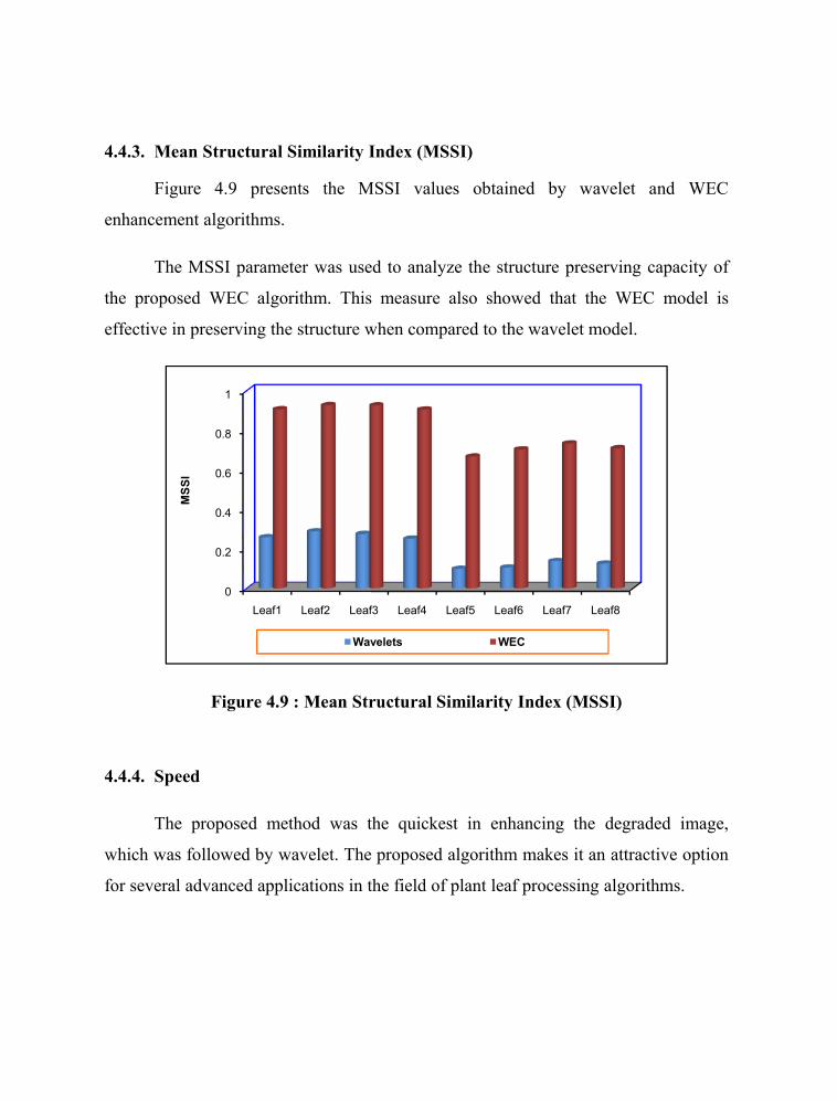
4.4.3. Mean Structural Similarity Index (MSSI)
Figure 4.9 presents the MSSI values obtained by wavelet and WEC
enhancement algorithms.
The MSSI parameter was used to analyze the structure preserving capacity of
the proposed WEC algorithm. This measure also showed that the WEC model is
effective in preserving the structure when compared to the wavelet model.
Figure 4.9 : Mean Structural Similarity Index (MSSI)
4.4.4. Speed
The proposed method was the quickest in enhancing the degraded image,
which was followed by wavelet. The proposed algorithm makes it an attractive option
for several advanced applications in the field of plant leaf processing algorithms.
0
0.2
0.4
0.6
0.8
1
Leaf1 Leaf2 Leaf3
MSS
I
Wavelets
83
4.4.3. Mean Structural Similarity Index (MSSI)
Figure 4.9 presents the MSSI values obtained by wavelet and WEC
enhancement algorithms.
The MSSI parameter was used to analyze the structure preserving capacity of
the proposed WEC algorithm. This measure also showed that the WEC model is
effective in preserving the structure when compared to the wavelet model.
Figure 4.9 : Mean Structural Similarity Index (MSSI)
4.4.4. Speed
The proposed method was the quickest in enhancing the degraded image,
which was followed by wavelet. The proposed algorithm makes it an attractive option
for several advanced applications in the field of plant leaf processing algorithms.
Leaf3 Leaf4 Leaf5 Leaf6 Leaf7 Leaf8
Wavelets WEC
83
4.4.3. Mean Structural Similarity Index (MSSI)
Figure 4.9 presents the MSSI values obtained by wavelet and WEC
enhancement algorithms.
The MSSI parameter was used to analyze the structure preserving capacity of
the proposed WEC algorithm. This measure also showed that the WEC model is
effective in preserving the structure when compared to the wavelet model.
Figure 4.9 : Mean Structural Similarity Index (MSSI)
4.4.4. Speed
The proposed method was the quickest in enhancing the degraded image,
which was followed by wavelet. The proposed algorithm makes it an attractive option
for several advanced applications in the field of plant leaf processing algorithms.

84
Original Images Wavelet WEC
Leaf 1
Leaf 2
Leaf 3
Leaf 4
Figure 4.10: Visual Results of Noise Removal (Standard Dataset)

85
Figure 4.11 : Visual Results of Noise Removal (Real Dataset)
Original Images Wavelet WEC
Leaf 5
Leaf 6
Leaf 7
Leaf 8
86
4.4.5 Visual Results
The visual comparison of the enhanced image produced by the proposed
algorithm for figure 3.2 and 3.3 is shown in Figure 4.10 and Figure 4.11 for the
standard and real datasets respectively and the results of the entire dataset is shown in
Appendix B. From the visual results, it is further confirmed that the enhancement
operations are successful and have improved the conventional wavelet based method.
4.5. CHAPTER SUMMARY
Leaf image enhancement is a vital preprocessing step in CAP-LR system.
This chapter introduced an automatic contrast adjustment, edge enhancement and
noise removal algorithm. The algorithm used CLAHE, relaxed median filter and
sigmoid function during the enhancement task. The experimental results showed that
the proposed method shows significant improvement in terms of noise removal, edge
preservation and speed. Thus, the various results of the experiments conducted clearly
indicate that the images produced by the proposed algorithm are of good visual quality
and therefore can be applied to CAP-LR system.
Recommended