Combinatorial and Computational GeometryMSRI PublicationsVolume 52, 2005
Binary Space Partitions:
Recent Developments
CSABA D. TOTH
Abstract. A binary space partition tree is a data structure for the rep-resentation of a set of objects in space. It found an increasing number ofapplications over the last decades. In recent years, intensifying researchfocused on its combinatorial properties, which affect directly the efficiencyof applications. Important advances were made on binary space partitionsfor disjoint line segments in the plane and for axis-aligned objects in higherdimensions. New research directions were also initiated on some realisticpolygonal scenes and on kinetic binary space partitions. This paper at-tempts to give an overview of these results and reiterates some of the mostpressing open problems.
1. Introduction
The binary space partition tree is a geometric data structure obtained by a
recursive partitioning scheme, called binary space partition (for short, BSP) over
a set of input objects: The space is partitioned along a hyperplane into two
half-spaces, then either half-space is partitioned recursively until every subprob-
lem contains only a trivial fraction of the input objects. The concept of BSP
has emerged from the computer graphics community in the seventies. It was
originally designed to assist efficient hidden-surface removal algorithms for mov-
ing viewpoints, but it has later found widespread applications in many areas of
computational and combinatorial geometry.
In many of the applications, the bottle neck of the space complexity is the size
of the BSP tree they rely on. Combinatorial research focused on determining
the worst case complexity of BSPs for certain classes of inputs. Despite the
simplicity of the BSP algorithm, it is often challenging to determine the so-
called partition complexity even for simple object classes such as disjoint line
segments in the plane, or axis-aligned boxes in higher dimensions. Ideally, the
partition hyperplanes do not split the input objects, and the size of the BSP tree
is linear in terms of the input size. In many cases, however, it is inevitable that
529
530 CSABA D. TOTH
input objects are also fragmented, and the size of the data structure becomes
superlinear.
This paper surveys results on the combinatorial properties of BSPs from the
last four-five years. Inevitably, we include less recent results as well because
early ideas and observations are often used, sometimes in an enhanced form,
to obtain new results. Before we move on to the latest developments, let us
define the binary space partition and the partition complexity, and recall a few
applications and early results.
Definitions. A binary space partition tree is a recursive partition scheme for
an input set of pairwise interior disjoint objects in Rd, d ∈ N. If the input
contains two full-dimensional objects or a lower-dimensional object, we partition
the space by a hyperplane h and recursively apply two binary space partitions
for the objects clipped in each of the two open half-spaces of h. If the input is
at most one full-dimensional object (and no lower-dimensional object), we stop.
The partition algorithm naturally corresponds to a binary tree: Every node
corresponds to the input of a recursive call of the BSP: The root corresponds to
the initial input set, the two children of a non-leaf node correspond to the inputs
of its two subproblems. The BSP tree data structure is based on this binary
tree: Every leaf stores at most one full-dimensional object which is the input
of the corresponding subproblem; and every non-leaf node stores the splitting
hyperplane and the (lower-dimensional) objects of the corresponding subproblem
that lie on the splitting hyperplane. As a convention, the non-leaf nodes store
only k-dimensional fragments of k-dimensional objects lying on the splitting
hyperplane in Rd, 0 ≤ k ≤ d. For example, if a splitting hyperplane h crosses
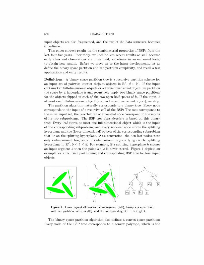
an input segment s then the point h ∩ s is never stored. Figure 1 depicts an
example for a recursive partitioning and corresponding BSP tree for four input
objects.
a
bc
d a1
b1
c
d
`1
`2
`3
`4
`5
a2
b2
`1
`2 `3, d
`4 `5 a2
a1 b1 b2 c
∅
Figure 1. Three disjoint ellipses and a line segment (left), binary space partition
with five partition lines (middle), and the corresponding BSP tree (right).
The binary space partition algorithm also defines a convex space partition:
Every node of the BSP tree corresponds to a convex polytope, which is the
BINARY SPACE PARTITIONS: RECENT DEVELOPMENTS 531
intersection of the halfspaces bounded by the splitting hyperplanes of its ances-
tors. The root corresponds to the space Rd. A splitting hyperplane stored at a
non-leaf node splits the corresponding convex polytope into the two polytopes
corresponding to the two child nodes. The polytope corresponding to a node is
also called the cell of the (sub)problem because it contains every input object of
the (sub)problem. Observe that the set of all leaves of a BSP tree correspond to
a convex partition of the space.
An important special BSP, called autopartition, is defined for at most (d−1)-
dimensional input objects in Rd. An autopartition is a BSP where every splitting
hyperplane contains an input object of the corresponding (sub)problem.
A BSP has two important parameters: Its size is the total number of fragments
of objects stored at the nodes of the BSP tree; its height is the height of the BSP
tree. The BSP in Figure 1 has size 6 and height 3. An easy way to compute
the size of the BSP is to sum the number of input objects and the number of
cuts, the events when a splitting hyperplane partitions (a fragment of) an input
object. If the BSP does not make “useless cuts”, that is, if every splitting plane
partitions the convex hull of the input objects, then the BSP size is an upper
bound on the number of non-leaf nodes of the BSP tree.
There are many BSPs for every input set depending on the choice of the
splitting hyperplane at each subproblem. The partition complexity of a set S of
objects is the size of the smallest BSP for S. The minimal size BSP does not
necessarily comes with minimal heights, though. The autopartition complexity of
a set S is the size of the smallest autopartition for S. Clearly, the autopartition
complexity is never smaller than the partition complexity.
The convention that objects lying in a partition hyperplane are not partitioned
further leads to somewhat counterintuitive phenomenon: A set of objects in Rd
with superlinear partition complexity will have linear partition complexity when
embedded into Rd+1 because a single splitting hyperplane contains them all. One
may define another binary partitioning scheme which would partition recursively
the fragments of objects lying in each splitting hyperplane. The minimal number
of fragments under such an alternative partition scheme may be much higher than
the partition complexity. In this survey, we focus on combinatorial properties of
the partition complexity.
1.1. Applications. The initial and most prominent applications, where the
BSP tree itself is stemming from, lie in computer graphics: BSPs support fast
hidden-surface removal [Schumacker et al. 1969; Fuchs et al. 1980; Murali 1998]
and ray tracing [Naylor and Thibault 1986] for moving viewpoints. Rendering
is used for visualizing spatial opaque surfaces on the screen. A common and
efficient rendering technique is the so-called painter’s method. It draws every
object sequentially according to the depth order or back-to-front order, starting
with the deepest object and proceeding with the objects closer to the viewer.

532 CSABA D. TOTH
When all the objects have been drawn, every pixel represents the color of the
object closest to the viewpoint.
Figure 2. Objects may have cyclic overlaps.
Unfortunately, some sets of objects have cyclic overlaps, where no valid depth
order exists (Figure 2). A BSP partitions the input objects into fragments for
which the depth order always exists for every viewpoint. It is easy to extract
the depth order of the fragments by a simple traversal of the BSP tree. An
additional benefit of BSPs is that the depth order can easily be updated as the
viewpoint moves continuously: It is enough to swap the two children of a node of
the BSP tree when the viewpoint crosses the corresponding splitting hyperplane.
(Computing the depth order, if it exists, for a fixed viewpoint may be easier than
constructing a BSP, however; see [de Berg 1993].)
The first applications of BSPs were soon followed by many others, e.g., con-
structive solid geometry [Thibault and Naylor 1987; Naylor et al. 1990; Buchele
1999] and shadow generation [Chin and Feiner 1989; Batagelo and Jr. 1999]. The
BSP for the faces of a full dimensional polyhedral solid can represent the solid
and its boundary with Boolean set operations. This, in turn, can be used for
efficient real-time shadow generation by computing the union of shadow volumes
obtained from traversals of the BSP tree in depth order for each light source
position. BSPs were also used in surface simplification [Agarwal and Suri 1998;
Shaffer and Garland 2001; Pauly et al. 2002] for clustering sample points.
Other applications of BSP trees include range counting [Agarwal and Ma-
tousek 1992], point location [Arya et al. 2000; de Berg 2000], collision detection
[Ar et al. 2000; Ar et al. 2002], robotics [Ballieux 1993], graph drawing [Asano
et al. 2003], and network design [Mata and Mitchell 1995]. BSP trees gen-
eralize some of the most commonly used geometric search structures such as
quadtrees/octrees, Kd-trees, and BAR-trees [Duncan et al. 2001], each of which
has numerous applications on its own right.
Early research. Research on combinatorial properties of BSPs began with
two influential papers of Paterson and Yao [1990; 1992]. They considered BSPs
for disjoint (d − 1)-dimensional hyper-rectangles in Rd (including line segments
in the plane). Many of their initial observations (about free cuts, anchored seg-
ments, and round-robin algorithms) are key elements of the most recent partition
algorithms, as well.

BINARY SPACE PARTITIONS: RECENT DEVELOPMENTS 533
Paterson and Yao [1990] gave a randomized and a deterministic algorithm
to construct a BSP of size O(n log n) and height O(log n) for n disjoint line
segments in the plane. The height bound is optimal apart from a constant
factor, but the size bound is not known to be tight. A lower bound construction,
where the partition complexity of n disjoint line segments is Ω(n log n/ log log n),
is discussed in Section 3.
They also proved that the partition complexity of n disjoint (d−1)-dimensional
simplices in Rd, d ≥ 3, is O(nd−1), which is best possible for d = 3 and tight for
autopartitions in every dimension [Paterson and Yao 1990]. In three-space, there
are n disjoint line segments, lying along a hyperbolic paraboloid, whose partition
complexity is Θ(n2). The same lower bound carries over to hyper-rectangles in
Rd with the same Θ(n2) partition complexity. The gap between the upper and
lower bounds in higher dimensions has resisted research efforts so far.
Open Problem. What is the partition complexity of n disjoint (d − 1)-dimen-
sional simplices in Rd, for d ≥ 4?
Every BSP computes a convex partition of the free space around the input ob-
jects. The size of the convex partition is the number of leaves of the BSP tree.
The partition complexity of (d−1)-dimensional simplices is, therefore, cannot be
smaller than the minimum convex partition of a polyhedron with n faces in Rd.
It would be tempting to derive lower bounds on the BSP size from the convex
partitioning, unfortunately, no super-quadratic lower bound is known for this
problem [Chazelle 1984] for any d ∈ N.
Open Problem. What is the size of a minimum convex partition of a polyhedron
with n faces in Rd, d > 3?
In this survey we focus on the worst case (maximum) partition complexity of a
set of objects of a certain type. Computation or approximation of the optimal
size BSP for specific instances seems to be an elusive open problem (see e.g.,
[Agarwal et al. 2000c]).
Open Problem. Is it NP-hard or is there a polynomial algorithm to compute
the partition complexity of n given disjoint line segments in the plane?
Open Problem. Is it APX-hard or is there a polynomial time approximation
scheme to compute the partition complexity of n given disjoint line segments in
the plane?
Road map. In Section 2, we continue with recalling earlier ideas and observa-
tions which proved to be omnipresent in later results on BSPs. This section can
be considered a short warm up course on the basics on binary space partitioning,
which is essential in understanding the sometimes intricate partition schemes
and lower bound constructions. Section 3 sketches the proof for two closely
related results on disjoint line segments in the plane: An Ω(n log n/ log log n)
lower bound construction and a constructive upper bound on segments with k

534 CSABA D. TOTH
distinct orientations, k ∈ N. Section 4 gathers a series of results about BSPs for
axis-aligned input objects, where all splitting hyperplanes are also axis-aligned.
We conclude the paper with two short sections related to other fields of com-
putational geometry: Section 5 reviews results on realistic object classes which
sometimes allow for linear partition complexity. Section 6 deals with kinetic
BSPs for continuously moving input objects.
2. Preliminaries
Many of the resent results on BSPs are based on or are extending basic con-
cepts known for decades. In this section, we present the most important ideas
with references the their recent extensions or enhancements.
Free cuts. A hyperplane h that does not split any input object but partitions
the set of objects into smaller sets (i.e., at least two of int(h−), h, and int(h+)
intersect input objects), is called a free cut. A minimum size BSP should use
free cuts whenever they are available [Paterson and Yao 1990]. A BSP that uses
free cuts only is called perfect. De Berg, de Groot, and Overmars [de Berg et al.
1997a] designed an O(n2 log n) time algorithm to detect if a perfect BSP exists
for n disjoint lien segments in the plane.
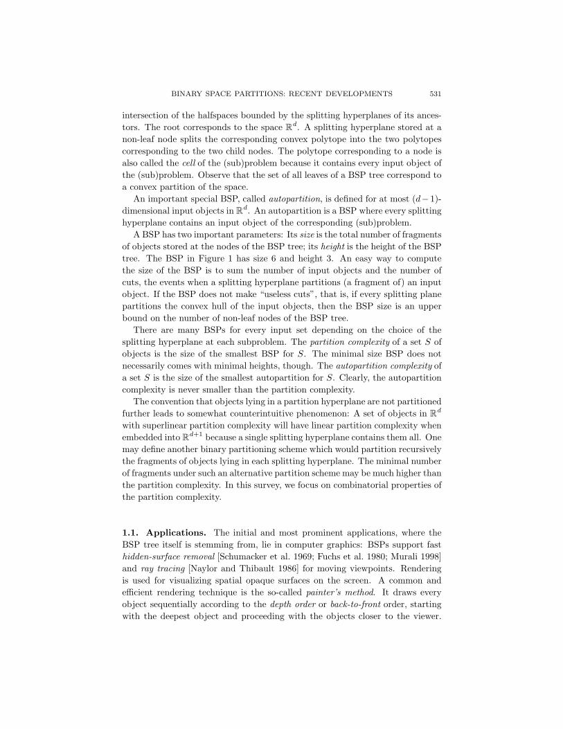
Cutting along a (d − 1)-dimensional object whose (relative) boundary lies
on the boundary of the cell is clearly a free cut (Figure 3). In the plane, this
implies, for instance, that if segment s is cut already at points p and q, then the
subproblem containing the middle fragment pq ⊂ s can be partitioned along pq
without cutting any input segment. Therefore, if we track the cuts of a single
input segment through an optimal binary space partitioning, then only the two
endings (the portion between the segment endpoint and the first or last cut) can
be further fragmented. This observation leads to an O(n log n) upper bound on
the partition complexity of n disjoint line segments [Paterson and Yao 1990], but
it is a basic element in all BSP algorithms.
Free cuts along objects. Consider a (d − 1)-dimensional object s in Rd. If a
fragment s of s is bounded by cuts (previous splitting planes), then a hyperplane
along s is a free cut for the subproblem containing s. As a consequence, we can
assume that whenever a splitting hyperplane cuts a fragment s of s then s is
adjacent to the (relative) boundary of s. If a splitting hyperplane h partitions
s but does not partition the common (relative) boundary of s and s ⊂ s (e.g.
in Figure 3), then this commmon boundary is entirely on one side of h and the
fragment of s on the other side of h is bounded by cuts and so it is a free cut.
For each final fragment of s adjacent to the boundary of s, there is one such cut
on every level of the BSP tree. Therefore the partition complexity of n disjoint
(d− 1)-dimensional simplices in Rd is upper bounded by the product of the size
and the height of a BSP for their (d − 2)-dimensional boundary simplices. For
BINARY SPACE PARTITIONS: RECENT DEVELOPMENTS 535
example, we obtain an O(n log n) size BSP for n disjoint line segments in the
plane from a 2n size and dlog 2ne height Kd-tree of the 2n segment endpoints.
h1h2 h3
ss
Figure 3. An input triangle s in R3 is cut by three vertical splitting planes h1,
h2, and h3. The striped triangle fragment is a free cut for the cell bounded by
the three splitting planes.
Paterson and Yao [1990] showed that cutting along all input objects in a
random order and applying free cuts whenever possible results in an O(nd−1)
expected size BSP for n disjoint (d−1)-dimensional simplices in Rd, d ≥ 3. This
BSP, however, can have linear expected height in the worst case, e.g., if the input
is the face set of a convex polytope. In three-space, this gives a randomized BSP
of O(n2) size and O(n) height for n disjoint triangles.
We can construct deterministically a BSP of O(log2 n) height and O(n2 log2 n)
size: Project all triangle edges to the xy-plane, and cover them with O(n2) pair-
wise non-crossing segments. By [Paterson and Yao 1990], there is a O(n2 log(n2))
size and O(log(n2)) height BSP for these segments. The lifting of the planar
splitting lines to vertical splitting planes in R3 along with all possible free cuts
gives a BSP for the triangles. Refining this idea, Agarwal et al. [2000c] designed
a BSP of size O(n2 log2 n) size and O(log n) height for n disjoint triangles; while
Agarwal, Erickson, and Guibas [Agarwal et al. 1998] reported a randomized BSP
of expected O(n2) size and O(log n) height.
Cycles. Assume that we are given disjoint (d − 1)-dimensional objects in Rd.
If the hyperplane spanned by any object is disjoint from all other objects, then
every hyperplane through an object is a free cut and we obtain a perfect BSP
of size n by partitioning along them in an arbitrary order. We can define a
binary relation between two objects a and b saying that a b if and only if the
hyperplane through a splits b. A BSP of size n using free cuts only still exists
if is an acyclic relation: No object is cut if we always split the space along a
minimum element with respect to . Sets with large partition complexity ought
to have many cycles w.r.t. . Figure 4 depicts examples of cycles in the plane
and in three space. Cycles are vital in the analysis of BSPs for disjoint line
segments in the plane.

536 CSABA D. TOTH
Anchored segments. A line segment is anchored if one of its endpoints lies
on the boundary of the cell. An anchored segment has only a uni-directional
extension that might split other segments. Paterson and Yao [1992] found a small
BSP for axis-aligned anchored segments in the plane that cuts non-anchored
segments at most four times. Using this BSP as a subroutine inductively, they
obtain an O(n) size BSP for n disjoint axis-parallel line segments: If a segment
is partitioned into c pieces during a BSP for anchored segments, then c−2 pieces
are free-cuts in their proper subproblems and are not fragmented any further,
the remaining two pieces are anchored and are taken care of by the next call of
the subroutine for anchored segments. This idea was extended and turned out
to be extremely fruitful in a number of recent results [Toth 2003b; Toth 2003a]
Figure 4. A set of line segments with a free cut and two cycles, one of which
is an anchored cycle (left). Axis-aligned rectangles where defines a complete
bipartite graph (right).
De Berg et al. [1997b] noticed a useful property of cycles of anchored segments.
Consider a cycle (a1, a2, . . . , ak) of anchored segments, where ai ai+1 for i =
1, 2, . . . , k−1 and ak a1. Assume, furthermore, that the first anchored segment
hit by the extension of ai is ai+1 for i = 1, 2, . . . k−1, and a1 for i = k (Figure 4).
A cycle cut for (a1, a2, . . . , ak) is a partition subroutine where we cut sequentially
along the segments ak, ak−1, . . . , a1 in this order. Note that only the first splitting
line can cut anchored segments. Indeed, ak−1 ak, so the extension of ak−1 hits
ak. The split along ak−1 does not extend beyond ak, along which we have made
a previous cut. Similarly, partitions along ak−2, . . . , a2, a1 are all free cuts w.r.t.
anchored segments of the initial problem. This property of cycles of anchored
segments in the plane unfortunately does not generalize to higher dimensions.
One possible higher dimensional generalization of anchored segments was in-
troduced by Dumitrescu et al. [2004] in the context of BSPs for axis-aligned
k-flats in Rd. An axis-aligned k-flat b is called an `-stabber, 0 ≤ ` ≤ k, if two
opposite (k − `)-faces of b lie on the boundary of the convex hull. Toth [2003a]
defined another generalization: A 1-stabber b is a shelf with respect to a cell C
if C \ b is simply connected. He showed that the partition complexity of shelves
is O(n log n) in R3.
BINARY SPACE PARTITIONS: RECENT DEVELOPMENTS 537
Round-robin partition. Researchers tried to construct small size BSPs by
computing, for each subproblem, a splitting plane that optimizes some objective
function [Paterson and Yao 1992; Nguyen 1996; Nguyen and Widmayer 1995].
Intuitively, an “optimal” cut should cut few objects and partition the input into
almost equal size subproblems. Local optimization rarely lead to near optimal
BSPs, one notable exception is the case of axis-parallel segments in Rd, d ≥ 3.
Paterson and Yao [1992] considered the product of the number of segments for
each axis-parallel direction as an objective function. They showed that locally
optimal axis-aligned cuts (i.e., cuts decreasing maximally this value) build up
to an O(nd/(d−1)) size and O(log n) height BSP, which is best possible. The
orientation of optimal axis-aligned cuts in recursive calls varies in an irregular
order.
A simple but efficient round-robin BSP scheme for axis-aligned objects in Rd
works in rounds: Each round partitions the space into 2d pieces in d recursive
steps along axis-aligned hyperplanes of all d orientations. The round-robin BSP
scheme for points in Rd is the well known Kd-tree. For axis-aligned line segments
in Rd, a round-robin BSP makes a cut recursively along the median hyperplanes
of the segment endpoints. This BSP has O(n(d−1)/d) size and O(log n) height,
which is best possible for n axis-aligned segments [Paterson and Yao 1992]. Re-
cently, round-robin schemes [Dumitrescu et al. 2004; Hershberger et al. 2004]
lead to non-trivial bounds on the axis-aligned partition complexity of (disjoint)
k-flats in Rd for certain values of k.
3. Line Segments in the Plane
The best known upper bound on the partition complexity of n disjoint line seg-
ments in the plane is O(n log n). Paterson and Yao [1990] found an astonishingly
simple randomized BSP of expected O(n log n) size. The trapezoid decomposi-
tion method of Preparata [1981] (see also [Preparata and Shamos 1985]) gives
a deterministic BSP of this size as well. It was widely believed that disjoint
segments in the plane have linear partition complexity, this was supported by
experiments and by linear upper bounds for certain input classes such as axis-
parallel segments [Paterson and Yao 1992], anchored segments, and segments of
similar length [de Berg et al. 1997b]. Toth [2003c] gave a family of n disjoint line
segments for every n, n ∈ N, whose partition complexity is Θ(n log n/ log log n).
An extension of these ideas lead to an O(n log k) bound on the partition com-
plexity of n disjoint line segments with k distinct orientations.
Lower bound construction. We show how the idea of cycles over segments
in the plane can be developed into a lower bound construction whose partition
complexity is Θ(n log n/ log log n). For the sake of simplicity, we focus on au-
topartitions, where every cut is made along an input segment. We start with the
simple observation that a BSP cuts at least one segment of every cycle. If every

538 CSABA D. TOTH
segment appears in a unique cycle of size 3, then this already implies that the
partition complexity of n segments is at least n + n/3. To guarantee a higher
rate of fragmentation we design a recursive construction on k levels: The con-
struction Si on level i, 1 < i ≤ k, consists of copies of the construction Si−1 of
level i − 1. On the lowest level, S0 consists of a single line segment.
We squeeze Si−1 into a long and skinny rectangle, and build congruent copies
of this deformed Si−1 into Si. Note that the partition complexity is invariant
under affine transformations. The copies of Si−1 are so skinny that their position
in Si can be described by disjoint line segments, which we call sticks. The lower
bound on the partition complexity depends on three elements: (a) If Si consists
of x copies of Si−1 arranged in cycles then we can guarantee that any BSP makes
at least Ω(x) cuts on sticks. (b) If a cut of a stick (that is, a cut through a copy of
Si−1) implies that Ω(|Si−1|) true segments of Si−1 are cut, then the arrangement
of sticks at level i actually guarantees Ω(n) cuts on the input segments. (c) Once
we make sure that cycles of sticks at distinct levels induce distinct cuts on each
input segment, then the entire construction gives a lower bound of Ω(kn) on the
partition complexity, where k is the number of levels. It remains to show how
to find a construction satisfying all three conditions with k = Ω(log n/ log log n)
levels.
Figure 5. A cycle (left) and two cycles composed of cycles enclosed in long and
skinny boxes (middle and right). A line spanned by segments in one rectangle
either pierces a cycle in another rectangle (middle) or not (right).
A splitting line ` intersecting a copy of Si−1 does not necessarily cut all the
true segments in Si−1. If ` cuts all sub-constructions Si−2 within Si−1, then it
destroys the cycle arrangement of the sticks in Si−1 (Figure 5, middle) and so
this cycle arrangement does not induce any cuts on segments of Si−1. Therefore
we assume that the sticks of Si−1 are arranged so that no line ` spanned by an
input segment in another copy of Si−1 destroys their cycle (Figure 5, right). If,
however, a line ` cuts only a fixed fraction ci−1, 0 < ci−1 < 1, of the sticks of
Si−1, then it cuts only(∏i
j=1 cj
)
· n true segments. Since we want∏k
i=1 ci to
be a constant independent of k = Ω(log n/ log log n), a cut through Si−1 must
BINARY SPACE PARTITIONS: RECENT DEVELOPMENTS 539
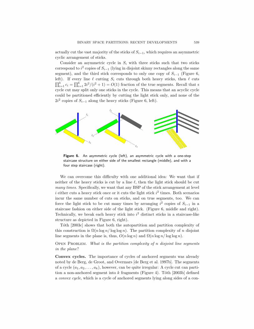
actually cut the vast majority of the sticks of Si−1, which requires an asymmetric
cyclic arrangement of sticks.
Consider an asymmetric cycle in Si with three sticks such that two sticks
correspond to i2 copies of Si−1 (lying in disjoint skinny rectangles along the same
segment), and the third stick corresponds to only one copy of Si−1 (Figure 6,
left). If every line ` cutting Si cuts through both heavy sticks, then ` cuts∏k
i=1 ci =∏k
i=1 2i2/(i2 + 1) = O(1) fraction of the true segments. Recall that s
cycle cut may split only one sticks in the cycle. This means that an acyclic cycle
could be partitioned efficiently by cutting the light stick only, and none of the
2i2 copies of Si−1 along the heavy sticks (Figure 6, left).
`1
`2
`1
`2
`3
Figure 6. An asymmetric cycle (left), an asymmetric cycle with a one-step
staircase structure on either side of the smallest rectangle (middle), and with a
four step staircase (right).
We can overcome this difficulty with one additional idea: We want that if
neither of the heavy sticks is cut by a line `, then the light stick should be cut
many times. Specifically, we want that any BSP of the stick arrangement at level
i either cuts a heavy stick once or it cuts the light stick i2 times. Both scenarios
incur the same number of cuts on sticks, and on true segments, too. We can
force the light stick to be cut many times by arranging i2 copies of Si−1 in a
staircase fashion on either side of the light stick. (Figure 6, middle and right).
Technically, we break each heavy stick into i2 distinct sticks in a staircase-like
structure as depicted in Figure 6, right).
Toth [2003c] shows that both the autopartition and partition complexity of
this construction is Ω(n log n/ log log n). The partition complexity of n disjoint
line segments in the plane is, thus, O(n log n) and Ω(n log n/ log log n).
Open Problem. What is the partition complexity of n disjoint line segments
in the plane?
Convex cycles. The importance of cycles of anchored segments was already
noted by de Berg, de Groot, and Overmars [de Berg et al. 1997b]. The segments
of a cycle (a1, a2, . . . , ak), however, can be quite irregular: A cycle cut can parti-
tion a non-anchored segment into k fragments (Figure 4). Toth [2003b] defined
a convex cycle, which is a cycle of anchored segments lying along sides of a con-

540 CSABA D. TOTH
vex polygon (Figure 7). Cutting sequentially along segments of a convex cycle
partitions any non-anchored segment into at most four pieces. To make sure
that every set of segments in a cycle contains a subset forming a convex cycle,
we drop the condition that ak a1 in the definition of convex cycles (Figure 7,
right).
b
b
b
a
a
bab
s
1
3
3
5
4
2 2
1
Figure 7. A convex cycle (a1, a2, a3) and a cycle (b1, b2, . . . , b5) that contains
a convex cycle (b1, b2, b3) with b3 6 b1.
Limited number of line directions. Paterson and Yao [1992] proved, us-
ing anchored segments, that the partition complexity of n disjoint axis-parallel
segments in the plane is at most 3n. This was further improved to 2n − 1 [Du-
mitrescu et al. 2004] (see Section 4). The proof techniques, however, do not
generalize for cases where the segments have three or more distinct orientations.
Toth [2003b] proved recently that for any k, k ∈ N, the autopartition complex-
ity of n disjoint line segments with k distinct orientations is O(nk), while their
partition complexity is O(n log k). The latter bound is asymptotically tight for
k = O(1) and also for the lower bound construction described above, that is,
where n disjoint segments have k = 2O(log n/ log log n) distinct orientations.
The partitioning algorithm for a set S of disjoint segments works in phases:
Every phase i performs a BSP for a fixed set Ai of anchored segments such that
no segment of S is cut more than O(log k) times (respectively, O(k) times in
the case of autopartitions). At an odd phase 2i − 1, we let A2i−1 be the set
of lower anchored segments at the current subproblem, that is, all (fragments
of) segments whose lower endpoint is on the boundary of a cell. Similarly, at
an even phase 2i, A2i is the set of all upper anchored segments. The result
follows immediately, since if a segment s ∈ S is cut in phase i then it is split into
c log k fragments, c log k− 2 of which are free cuts in their subproblem and 2 are
anchored fragments. The two endings of s may be cut again O(log k) times in

BINARY SPACE PARTITIONS: RECENT DEVELOPMENTS 541
phase i + 1 and i + 2 during a BSP for upper and lower anchored segments, but
s is no longer cut in later phases.
A phase i calls a BSP subroutine P for the set Ai in each cell. P (Ai) makes
two types of cuts: (1) A segment-cut splits a cell along a line ` spanned by a
segment s ∈ Ai. It is applied if ` does not cut any anchored segment in the
cell. (2) A cycle-cut partitions along a convex cycle of anchored segments (as
described in Section 2). Every cycle-cut is followed by a cleanup step, where we
apply the subroutine P for subsets Bi ⊂ Ai of those anchored segments of Ai
which are split by the cycle cut. One can ensure that Bi has at most half as many
distinct orientations as Ai in each resulting subcell (in case of autopartitions, Bi
has at least one fewer distinct orientations than Ai in each subcell).
For every phase, the segment-cut and cycle-cut steps can be assigned into
different levels according to recursive calls where subroutine P applied them.
Since the number of distinct orientations decreases by a factor of two in each
level, there are at most log k levels (at most k levels for autopartitions). One can
also ensure by carefully isolating the region in which a cycle-cut splits anchored
segments of Ai that every input segment is cut O(1) times in each level. This
implies that every segment is cut at most O(log k) times in total (O(k) times for
autopartitions).
4. Axis-aligned Binary Space Partitions
A k-dimensional object is axis-aligned, if each of its `-dimensional faces is
parallel to ` coordinate axes, 1 ≤ ` ≤ k. In an orthogonal coordinate system,
axis-aligned objects are also called orthogonal, rectilinear, or isothetic. Note
that BSPs are invariant under affine transformations of the Euclidean space,
and so the partition complexity of axis-aligned objects is independent of the
angles among the coordinate axes. BSPs for axis-aligned objects are important,
because in many applications input objects are axis-aligned by nature or are
modeled by their axis-aligned bounding boxes.
The simplest axis-aligned objects are the boxes, defined as a cross product∏d
i=1[ai, bi] of d intervals in Rd. The extent dimensions of a box B are the
coordinates i where ai < bi, while in every non-extent dimension, ai = bi.
An axis-aligned k-flat is a box with k extent dimensions. An axis-parallel line
segment, for example, is a 1-flat.
Every partition algorithm in this section uses axis-aligned splitting hyper-
planes only, such BSPs are said to be axis-aligned. Note that every cell in an
axis-aligned BPS is an axis-aligned box. For most axis-aligned input classes,
the axis-aligned BSPs are best possible among all BSPs ignoring constant or
logarithmic factors, because they match the partition complexity known for the
class. In some cases, lower bounds known for axis-aligned BSPs are higher by a
constant or logarithmic factor than those for the general BSPs. Of course, it is
542 CSABA D. TOTH
easy to construct instances where the smallest BSP and the smallest axis-aligned
BSP have significantly different sizes.
Segments and rectangles in the plane. After Paterson and Yao [1992]
showed that the partition complexity of n disjoint axis-parallel line segments in
the plane is O(n), it remained to determine the exact value of the coefficient
hidden in the asymptotic notation. A partition algorithm due to d’Amore and
Franciosa [1992], originally designed for axis-aligned boxes, always computes an
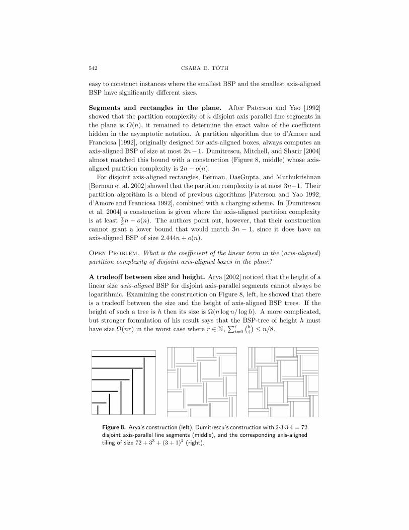
axis-aligned BSP of size at most 2n−1. Dumitrescu, Mitchell, and Sharir [2004]
almost matched this bound with a construction (Figure 8, middle) whose axis-
aligned partition complexity is 2n − o(n).
For disjoint axis-aligned rectangles, Berman, DasGupta, and Muthukrishnan
[Berman et al. 2002] showed that the partition complexity is at most 3n−1. Their
partition algorithm is a blend of previous algorithms [Paterson and Yao 1992;
d’Amore and Franciosa 1992], combined with a charging scheme. In [Dumitrescu
et al. 2004] a construction is given where the axis-aligned partition complexity
is at least 73n − o(n). The authors point out, however, that their construction
cannot grant a lower bound that would match 3n − 1, since it does have an
axis-aligned BSP of size 2.444n + o(n).
Open Problem. What is the coefficient of the linear term in the (axis-aligned)
partition complexity of disjoint axis-aligned boxes in the plane?
A tradeoff between size and height. Arya [2002] noticed that the height of a
linear size axis-aligned BSP for disjoint axis-parallel segments cannot always be
logarithmic. Examining the construction on Figure 8, left, he showed that there
is a tradeoff between the size and the height of axis-aligned BSP trees. If the
height of such a tree is h then its size is Ω(n log n/ log h). A more complicated,
but stronger formulation of his result says that the BSP-tree of height h must
have size Ω(nr) in the worst case where r ∈ N,∑r
i=0
(
hi
)
≤ n/8.
Figure 8. Arya’s construction (left), Dumitrescu’s construction with 2·3·3·4 = 72
disjoint axis-parallel line segments (middle), and the corresponding axis-aligned
tiling of size 72 + 33 + (3 + 1)2 (right).
BINARY SPACE PARTITIONS: RECENT DEVELOPMENTS 543
On the two extremities, this implies that an axis-aligned BSP-tree of size
O(n) has height nΩ(1); and one of height O(log n) has size Ω(n log n). The set of
segments in Arya’s construction, however, has linear partition complexity: All
segments become anchored after a diagonal cut (dotted line on Figure 8, left).
No tradeoff is known so far for the size and height of general BSP trees.
Open Problem. Is there a tradeoff between the size and the height of the BSP
trees for disjoint line segments (with arbitrary orientations)?
k-flats in d-dimensions. Paterson and Yao [1992] proved that the axis-aligned
partition complexity of n disjoint line segments in Rd, d > 2, lies between
(n/d)d/(d−1) + n and d · (n/d)d/(d−1) + n. There has been no improvement on
the coefficients on the main terms so far. Their lower bound construction is a
cubic grid∏d
i=11, 2, . . . , (n/d)1/(d−1) where d lines of distinct orientation stab
each grid cell. Their upper bound can be obtained by a round-robin partition
algorithm applying median cuts in all d directions.
Dumitrescu, Mitchell, and Sharir obtained an O(nd/(d−k)) upper bound for
the partition complexity of n axis-aligned k-flats in Rd [Dumitrescu et al. 2004].
It is not difficult to see that a round-robin cutting scheme delivers this bound,
too: Let every round consist of d recursive cuts in all d directions such that every
splitting hyperplane cuts through the median of the vertex set of the fragments
clipped to the cell. The total number of fragments may increase by a factor of
2k in each round, because every (fragment of a) k-flat can be split along each
of its k extents. At the same time, the number of fragments in one subproblem
decreases by a factor of 2d−k. So there are at most (log2 n)/(d − k) rounds,
and the BSP size is O(n · nk/(d−k)). Dumitrescu et al. [2004], in fact, applied a
somewhat different partition scheme where all cuts for each hyperplane direction
are made simultaneously. They also give a matching lower bound of Ω(nd/(d−k))
for the case where k < d/2.
The formula Θ(nd/(d−k)) is no longer valid for disjoint objects if k ≥ d/2 (the
axis-aligned partition complexity is Θ(n5/3) for k = 2 and d = 4 [Dumitrescu
et al. 2004]). The reason for this is that disjointness plays no role if k < d/2,
but it is restrictive for k ≥ d/2. Indeed, if two objects whose extent dimensions
together do not contain all d dimensions intersect, then they have a common non-
extent dimension where their coordinates coincide. Any system of k-flats in Rd,
k < d/2, can be perturbed into a pairwise disjoint set by translating each object
independently by a small random vector. If the random vectors are sufficiently
small, then this perturbation does not decrease the partition complexity (every
BSP for the perturbed set translates into a BSP of less than or equal size for
the original input). Two flats whose extent dimensions contain all d dimensions
may not always be separated by an arbitrarily small perturbation. The simplest
examples are a set of axis-parallel segments in the plane and in R3, respectively:
A small random perturbations removes all segment-segment intersection in three-
space, but intersections may prevail in the plane.

544 CSABA D. TOTH
The disjointness requirement is more apparent for the following generalization
of free cut segments in higher dimensions: An axis-aligned box is a stabber in
dimension i if its extent contains the extent of the bounding box of the input in
dimension i. It is an M-stabber for a set M ⊆ 1, 2, . . . , d, if it is a stabber in
every dimension i ∈ M ; we can also say that it is a k-stabber if k = |M |. An
M1-stabber and an M2-stabber intersect if M1 ∪ M2 = 1, 2, . . . , d. Stabbers
were defined by Dumitrescu, Mitchell, and Sharir [Dumitrescu et al. 2004]. Later
Hershberger, Suri, and Toth [Hershberger et al. 2004] gave an alternative defini-
tion saying that a box is k-stabber, if all its j-faces, j < k, lie on the boundary
of the bounding box.
The concept of stabbers is crucial in any axis-aligned BSP algorithm. Let us
mention just two of their useful properties: (i) A (d − 1)-stabber is a free-cut
in Rd. (ii) Apart from at most 2k fragments incident to the vertices of b, every
fragment of a k-flat b is a `-stabber for some 1 ≤ ` ≤ k. A set of disjoint stabbers
corresponds to a pairwise intersecting set system: Let us map every stabber b to
the set ϕ(b) ⊂ 1, 2, . . . , d of dimensions in which b is not a stabber. ϕ(b) : b is
a pairwise intersecting set system; and vice versa: Given a pairwise intersecting
set system D on 1, 2, . . . , d, there is a set of stabbers in Rd whose image under
ϕ is D.
Tilings. In every lower bound construction where the partition complexity is
high, the free space surrounding the input objects is also complex in the sense
that its smallest convex partition is often superlinear. Researchers expected
that if there is no space among the (convex) input objects (or, if the convex
partition of the free space has the same order of magnitude as the input), then
the partition complexity would be significantly smaller. A tiling in Rd is a set
of d-dimensional objects that partition the space. An axis-aligned tiling is a set
of full-dimensional axis-aligned boxes that partition the space.
Already in the plane, the worst case partition complexity of axis-aligned tilings
is smaller than that of disjoint boxes. Berman, DasGupta, and Muthukrishnan
[Berman et al. 2002] showed that every axis-aligned tiling of size n has an axis-
aligned BSP of size at most 2n (recall that the axis-aligned partition complexity
of disjoint rectangles is at least 73n − o(n) [Dumitrescu et al. 2004]). This is
asymptotically optimal, since a construction from [Dumitrescu et al. 2004], orig-
inally designed for disjoint line segments, can be converted to an axis-aligned
tiling. Their lower bound construction for axis-parallel line segments consists
of 2k(k + 1) bundles of k parallel lines (Figure 8, middle). These 2k3 + 2k2)
segments can be blown up to skinny axis-aligned boxes such that each bundle
fills an axis-aligned rectangle, and the free space between the rectangles can be
covered by k2 + (k + 1)2 = O(k2) interior-disjoint axis-aligned boxes (Figure 8,
right). A total of n = 2k3 + O(k2) boxes tile the plane, and their axis-aligned
BSP cannot be smaller than that of the original k3 segments we have started
with, that is, at least 4k3 − O(k2).

BINARY SPACE PARTITIONS: RECENT DEVELOPMENTS 545
The difference in the partition complexity of disjoint and plane filling rectan-
gles was only the coefficient of the linear term. In three- and higher dimensions
the upper bounds on the partition complexity of tilings is smaller in exponent
than that of disjoint boxes. Hershberger and Suri [2003] observed that every
tiling where all (d−3)-dimensional faces of every tile lie on the convex hull has a
linear size axis-aligned BSP. (This is not true for disjoint axis-aligned boxes, in
general: In the known worst-case constructions, all (d − 3)-dimensional faces lie
on the convex hull.) This implies that it is enough to partition an axis-aligned
tiling until every cell is empty of (d−3)-dimensional faces, and then a linear size
BSP in each cell results in a BSP for the input tiling.
Hershberger, Suri, and Toth [Hershberger et al. 2004] apply a round-robin
BSP for the (d − 3)-dimensional faces of an axis-aligned tiling in Rd. One can
show that the number of (d − 3)-faces in each subproblem decreases by a factor
of 23. Therefore the round-robin scheme terminates in 13 log n+O(1) rounds. In
each round of the round-robin scheme, every (d − 2)-face is split into at most
2d−2 fragments. In the course of 13 log n + O(1) rounds, every (d − 2)-face is
partitioned into (2d−2)1
3log n+O(1) = O(n(d−2)/3) fragments. Since the (d − 1)-
faces that become free-cut in their subproblem are not fragmented any further,
every (d − 1)-face and every tile is partitioned into O(n(d−2)/3) fragments, as
well. The round-robin scheme for (d − 3)-faces partitions the axis-aligned tiling
in Rd into n ·O(n(d+1)/3) = O(n(d+1)/3) fragments such that no (d− 3)-face lies
in the interior of a cell. By applying a linear size BSP for the tiling clipped in
each resulting cell, we obtain a BSP of size O(n(d+1)/3) for an axis-parallel tiling
with n tiles in Rd. By contrast, the best known upper bound on the partition
complexity of n disjoint full-dimensional boxes in Rd is O(nd/2) only.
In dimensions d = 3, the partition complexity of axis-aligned tilings of size
n is O(n4/3), which is tight by a construction of Hershberger and Suri [2003].
They start with the lower bound construction of Paterson and Yao [1992] for
axis-parallel line segments in three space, which consists of 3k2 axis-parallel line
segments such that three segments of distinct directions stab every unit cube
in [0, k] × [0, k] × [0, k] grid. Then they replace every segment by an air-tight
bundle of k axis-aligned skinny boxes, and fill the free space between the bundles
by 2k3 pairwise disjoint boxes. They obtain a tiling with n = 5k3 boxes. By
the argument of Paterson and Yao, each grid cell corresponds to a cut through
a bundle of k skinny boxes, which gives a total of k · k3 = Θ(n4/3) cuts of
tiles. Generalizing this idea and ideas of Dumitrescu et al. [2004], Hershberger,
Suri, and Toth [Hershberger et al. 2004] gave a construction in d-dimensions for
which the axis-aligned partition complexity is Ω(nβ(d)), where limd→∞ β(d) =
(1+√
5)/2 = 1.618. Apart from the staggering gap between the upper and lower
bounds for d ≥ 4, many problems remain open on BSPs of axis-aligned and of
general tilings.
546 CSABA D. TOTH
Open Problem. What is the (axis-aligned) partition complexity of n space
filling axis-aligned boxes in Rd, d ≥ 4?
Open Problem. What is the partition complexity of n space filling simplices in
Rd, d ≥ 3?
Open Problem. What is the partition complexity of n tetrahedra that form the
triangulation of a convex polytope in d-space, d ≥ 3?
Fat rectangles. Another characteristics of the lower bound constructions for
n axis-aligned rectangles in R3 is that the rectangles are long and skinny (they
are axis-parallel line segments fattened by a small ε > 0 in all extent dimen-
sions). It was reasonable to expect that disjoint fat objects have small partition
complexity. An axis-aligned k-flat is fat if the ratio of a largest inscribed and a
smallest circumscribed cubes1 in the k-dimensional space spanned by the object
is bounded by a constant.
De Berg [1995] proved that the partition complexity of full dimensional dis-
joint fat objects is linear in every dimension. This is true for any set of disjoint
fat objects even if they are not axis-aligned (Section 5 deals with further ex-
tensions of this result). On the other hand, n disjoint fat but not axis-aligned
rectangles may have Θ(n2) partition complexity [Paterson and Yao 1990].
Agarwal et al. [2000b; 1998] considered n disjoint axis-aligned fat 2-flats in R3
and proved that their partition complexity is n·2O(√
log n). Toth [2003a] improved
this upper bound and gave an algorithm to compute a BSP of O(n log8 n) size
and O(log4 n) height. He also gave a lower bound construction for which the
axis-aligned partition complexity is Ω(n log n).
The main difficulty in dealing with a fat rectangle r in three-space is that the
fragments of r clipped to a cell of a subproblem is not necessarily fat anymore.
Every fragment, however, belongs to one of the following three types, each of
which has some useful properties that help our partitioning algorithm.
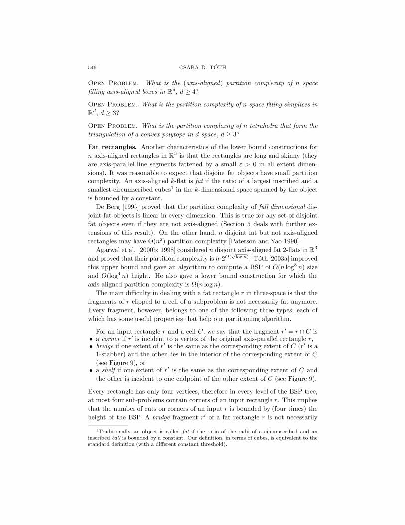
For an input rectangle r and a cell C, we say that the fragment r′ = r ∩ C is• a corner if r′ is incident to a vertex of the original axis-parallel rectangle r,• bridge if one extent of r′ is the same as the corresponding extent of C (r′ is a
1-stabber) and the other lies in the interior of the corresponding extent of C
(see Figure 9), or• a shelf if one extent of r′ is the same as the corresponding extent of C and
the other is incident to one endpoint of the other extent of C (see Figure 9).
Every rectangle has only four vertices, therefore in every level of the BSP tree,
at most four sub-problems contain corners of an input rectangle r. This implies
that the number of cuts on corners of an input r is bounded by (four times) the
height of the BSP. A bridge fragment r′ of a fat rectangle r is not necessarily
1Traditionally, an object is called fat if the ratio of the radii of a circumscribed and aninscribed ball is bounded by a constant. Our definition, in terms of cubes, is equivalent to thestandard definition (with a different constant threshold).

BINARY SPACE PARTITIONS: RECENT DEVELOPMENTS 547
Figure 9. Shelves, bridges, and free-cuts clipped to a cell C in R3.
fat. It still preserves part of the fatness of r, a property we call semi-fatness: If
r is α-fat then the extent of r′ in the interior of that of C is at most α times
longer than the extent containing the corresponding extent of C. The semi-
fatness allows us to separate bridges of different orientations (see subroutine P3
below). Finally, there is an O(n log n) size BSP for n disjoint shelves such that
it partitions every rectangle into at most O(log2 n) fragments.
We outline the main ideas to construct a O(log4 n) height BSP for disjoint
axis-aligned fat rectangles. The partition algorithm is composed of a four level
hierarchy of BSPs: We give a glimpse of each level and explain the lowest level
(a BSP for shelves) in detail below.
The main algorithm, P1, makes cuts recursively along the median xy-plane
of the vertices of the input rectangles. Since the number of rectangle vertices
in a cell is halved in each step, P1 terminates in O(log n) rounds. After every
median cut of P1, a cleanup step is applied in each cell C, which is a BSP for
the stabbers w.r.t. C and partitions every rectangle into O(log6 n) fragments. If
the cleanup step P2 makes a cut along a stabber r ∩C, then subsequent median
cuts of P1 cannot partition r ∩ C anymore. This ensures that the median cuts
performed by P1 may split any rectangle O(log n) times only.
The BSP P2 for a set S of stabbers makes cuts recursively along the median
xz-plane of the vertex set of S. Each median cut of P2 is followed by another
cleanup subroutine, P3, which in each cell separates the stabbers of S from other
stabbers (i.e., fragments that became stabbers due to the last median cut by
P2). Finally, P3 makes cuts along yz-planes, and calls a BSP P4 for all shelves
after every such step. We describe the BSP P4 for a set S of n shelves in a cell.
P4 has O(n log n) size and it partitions every rectangle into O(log n) fragments.
Consider a set S⊥ of n⊥ disjoint shelves in a cell C. Assume for simplicity
that they are all adjacent to the bottom side of C. The subroutine BSP for
S⊥ is a simple recursive algorithm: We split C by a horizontal plane h through
the highest upper edge of a shelf in S⊥, then we split the subcell below h along
the highest shelf (a free cut) and along the median shelf, and recursively call
this subroutine for each resulting subproblem (Figure 10 shows an example).
The algorithm terminates in log n⊥ rounds because the number of shelves in a
subproblem is halved in each round. None of the shelves is split, and we show that

548 CSABA D. TOTH
every axis-parallel segment disjoint from these shelves is cut O(log n⊥) times: A
segment parallel to stabbing extent of the shelves is never cut, a vertical segment
is cut at most once in every round, which amounts to O(log n⊥) cuts. Lastly,
consider a segment s orthogonal to the shelves. In subproblems where s is a
stabbing segment, it lies above the highest shelf and so it cannot be cut at all.
In a subproblem where an endpoint of s lies in the interior of a cell, s be cut by
the splitting planes along the median shelf, which totals to at most 2 log n⊥ cuts
during the entire subroutine.
Figure 10. First two rounds of the BSP for shelves.
This was a BSP for shelves along the one side of a cell C. We still need to
integrate six BSPs for each of the six sides of C: If we naıvely call the subroutine
six times sequentially for the subproblems and for each side then the number of
cuts on axis-parallel segments might be (O(log n))6. We use, instead, the concept
of overlay of BSPs to keep the number of cuts on every segment O(log n). We
compute independently six BSPs for the shelves adjacent to each side, then we
“overlay” them one after another: A cut along a splitting plane made in one BSP
may incur splits in several cells resulting from previous BSPs. The combination
is still a valid BSP because every subproblem is split by a hyperplane. The
number of cuts on each segment is the sum of the cuts made by each of the six
BSPs rather than their product. The overlay of BSPs is a key concept to keep
the number of cuts low throughout this algorithm.
In general we would like know the partition complexity of n disjoint axis-
aligned fat k-flats in Rd, 1 < k < d. It is easy to show a lower bound of
Ω(n(d−k+1)/(d−k)). Indeed, consider a worst case construction for n axis-parallel
line segments in Rd−k+1, whose partition complexity is Ω(n(d−k+1)/(d−k)) by
Paterson and Yao [1992]. Embed it into a (d−k+1)-dimensional affine subspace
H of Rd and expand it to a k-dimensional square orthogonally to H. We obtain
n pairwise disjoint k-dimensional squares in Rd. The size of any BSP for this
set is Ω(n(d−k+1)/(d−k)). We expect that this bound can be attained apart from
a polylogarithmic factor, that is, out of the k extents of a k-dimensional fat
rectangle, k − 1 extents are essentially redundant with respect to the partition
complexity.

BINARY SPACE PARTITIONS: RECENT DEVELOPMENTS 549
Open Problem. What is the (axis-aligned) partition complexity of n disjoint
fat axis-aligned k-flats in Rd, 1 < k < d?
5. From Fatness to Guardable Scenes
The worst case constructions for the partition complexity of general and axis-
aligned disjoint objects in 3-space use long and skinny input objects. This obser-
vation suggests that disjoint fat objects must have small partition complexity. A
full dimensional object is fat if the ratio of an circumscribed and inscribed ball
is bounded by a constant. Fat objects are often easier to handle. Among other
things, the union of fat objects have small combinatorial complexity in many
cases [Efrat and Sharir 2000; Pach and Tardos 2002; Pach et al. 2003]. A result
that every set of disjoint fat objects has linear partition complexity [de Berg
1995] initiated a flurry of work on extensions defining new object classes which
also have linear partition complexity by analogous arguments.
Fat full dimensional objects De Berg, de Groot, and Overmars [1997b] have
proved that the partition complexity of n disjoint convex fat objects in the plane
is O(n). De Berg [1995] has later found an elegant proof that establishes linear
partition complexity for disjoint full dimensional fat polyhedra with constant
number of vertices (e.g., fat tetrahedra) in Rd, d ∈ N, as well. His partition
algorithm generates the BSP tree in O(n log n) time for any d ∈ N, where the
constant of proportionality depends on the dimension. We briefly describe his
method below.
Consider an orthogonal coordinate system and then compute the axis-aligned
bounding box of every fat object. Generate a BSP for the set V of vertices of
all bounding boxes by repeating one of the following two steps starting with a
bounding cube C of V : (i) Partition the cubic cell C into 2d congruent cubes if
at least two sub-cubes have non-empty intersection with V . (ii) Otherwise every
point of V ∩C lies in one of the subcubes C ′. In this case, partition C along the
sides of the bounding cube of (V ∩C)∪c′ and (subsets of) where c′ is the common
vertex of C and C ′. Every subproblem that still contains a vertex of V is a cube
(allowing recursion). The subcells of the complement of the bounding box of
(V ∩C)∪ c′ in C are not necessarily fat but they can be expressed as the union
of O(1) cubes. Every cell of the resulting partition is empty of bounding box
vertices of the fat input objects. This implies that every resulting cell intersects
only a constant number of input objects. In each subproblem, one can complete
the BSP with a constant number of cuts if every fat object is either convex or
polyhedral with constant combinatorial complexity.
Note that the argument above used only that the input objects are fat, and
that they are pairwise disjoint. The extensions of disjoint fat scenes define prop-
erties of the whole input scene rather than properties of individual objects.
550 CSABA D. TOTH
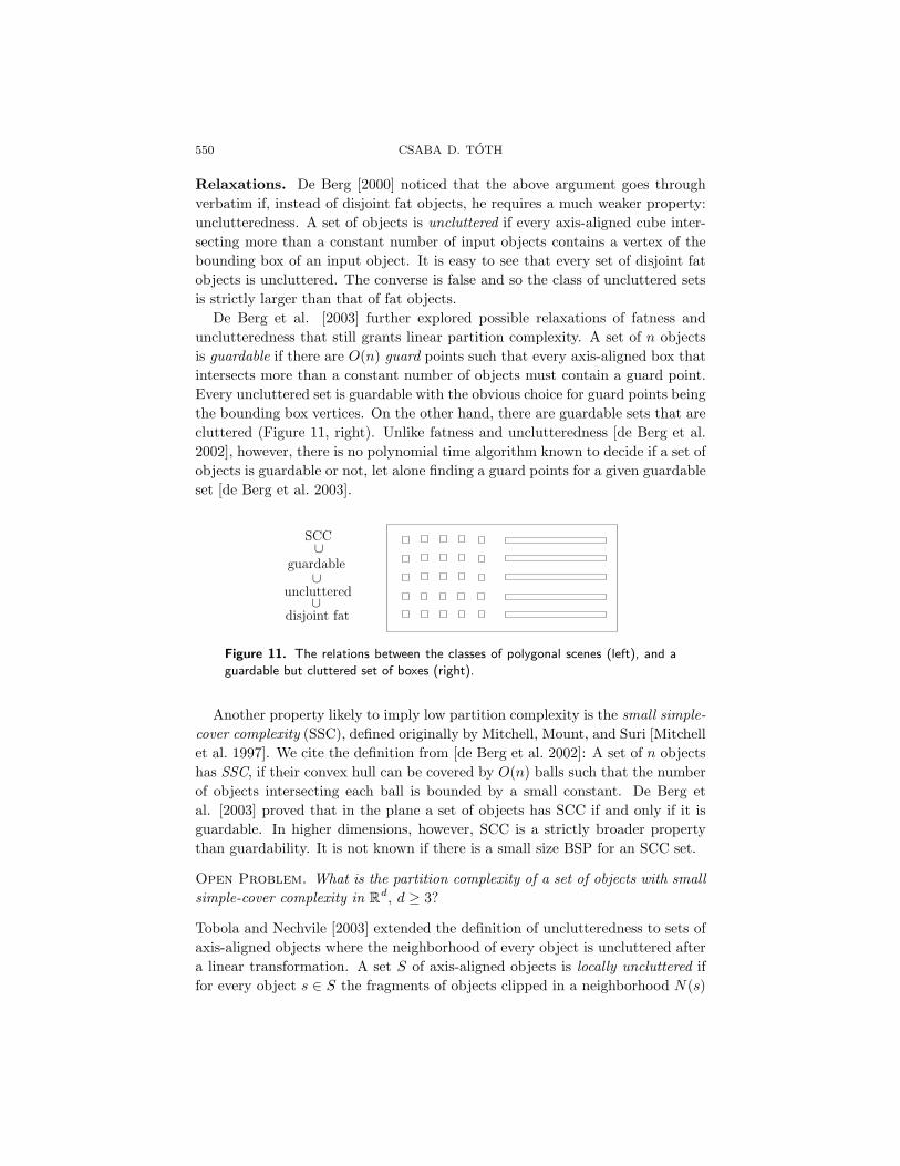
Relaxations. De Berg [2000] noticed that the above argument goes through
verbatim if, instead of disjoint fat objects, he requires a much weaker property:
unclutteredness. A set of objects is uncluttered if every axis-aligned cube inter-
secting more than a constant number of input objects contains a vertex of the
bounding box of an input object. It is easy to see that every set of disjoint fat
objects is uncluttered. The converse is false and so the class of uncluttered sets
is strictly larger than that of fat objects.
De Berg et al. [2003] further explored possible relaxations of fatness and
unclutteredness that still grants linear partition complexity. A set of n objects
is guardable if there are O(n) guard points such that every axis-aligned box that
intersects more than a constant number of objects must contain a guard point.
Every uncluttered set is guardable with the obvious choice for guard points being
the bounding box vertices. On the other hand, there are guardable sets that are
cluttered (Figure 11, right). Unlike fatness and unclutteredness [de Berg et al.
2002], however, there is no polynomial time algorithm known to decide if a set of
objects is guardable or not, let alone finding a guard points for a given guardable
set [de Berg et al. 2003].
uncluttered
disjoint fat
guardable
SCC
∪
∪
∪
Figure 11. The relations between the classes of polygonal scenes (left), and a
guardable but cluttered set of boxes (right).
Another property likely to imply low partition complexity is the small simple-
cover complexity (SSC), defined originally by Mitchell, Mount, and Suri [Mitchell
et al. 1997]. We cite the definition from [de Berg et al. 2002]: A set of n objects
has SSC, if their convex hull can be covered by O(n) balls such that the number
of objects intersecting each ball is bounded by a small constant. De Berg et
al. [2003] proved that in the plane a set of objects has SCC if and only if it is
guardable. In higher dimensions, however, SCC is a strictly broader property
than guardability. It is not known if there is a small size BSP for an SCC set.
Open Problem. What is the partition complexity of a set of objects with small
simple-cover complexity in Rd, d ≥ 3?
Tobola and Nechvile [2003] extended the definition of unclutteredness to sets of
axis-aligned objects where the neighborhood of every object is uncluttered after
a linear transformation. A set S of axis-aligned objects is locally uncluttered if
for every object s ∈ S the fragments of objects clipped in a neighborhood N(s)
BINARY SPACE PARTITIONS: RECENT DEVELOPMENTS 551
of s are uncluttered after a linear transformation Ts. The neighborhood N(s) is
the axis-aligned box obtained from s by fattening each extent with a multiple
of the longest extent of s. Tobola and Nechvile [2003] show that every locally
uncluttered set of n objects in Rd has an O(n) size axis-aligned BSP.
6. Kinetic Binary Space Partitions
The first motivation for binary space partitions was efficient hidden-surface
removal from a moving viewpoint. The input objects of the BSP were, however,
assumed to be static. Recent research on BSPs for moving objects was set in
the model of kinetic data structures (KDS) of [Basch et al. 1999]. In this model,
objects move continuously along a given trajectory (flight plan), typically along
a line or a low degree algebraic curve. The splitting hyperplanes are defined
by faces of the input objects, and so they move continuously, too. The BSP is
updated only at discrete events, though, when the combinatorial structure of the
BSP changes.
In the KDS paradigm, the goal is to maintain at all times a BSP whose size
and height is below a reasonable threshold, which is usually close to the partition
complexity available for static input. Efficiency of the algorithms are measured
by additional parameters: the total space required during the algorithm, total
time, which is broken down into the total number of events and the maximum
update time for an event.
First Agarwal et al. [2000c] studied the BSP in the KDS setting. They
consider n moving line segments in the plane such that the trajectory of every
segment endpoint is a constant degree polynomial and the segments are pairwise
disjoint at all times. They design a randomized algorithm to maintain a BSP of
expected size O(n log n) in O(n log n) space, the number of events is O(n2) and
each event requires an expected O(log n) update time.
Instead of adapting a previously known static BSP algorithm [Paterson and
Yao 1990] to KDS paradigm, they start out from a randomized incremental BSP,
which is an adaptation of the vertical (trapezoid) decomposition of Mulmuley
[1990] and Seidel [1991]. They fix a random permutation of the segments, which
is the only random choice in the algorithm. In their BSP, every splitting line
is either vertical or a free cut (i.e., lies along an input segment); they call such
BSPs cylindrical. By restricting the possible splitting planes, they reduce the
number of possible event types: In fact, the only possible combinatorial event
is that a segment endpoint starts or stops crossing a vertical splitting line. A
careful analysis of the effects of these events on the BSP tree establishes the
bounds on the update time and the total space requirement.
All known kinetic BSPs are based on vertical decomposition. This choice keeps
the types of the possible combinatorial events under control, but the number of
events can be suboptimal. If the x coordinates of every two segment endpoints
are swapped during the motion, then the number of events can be Θ(n2) for any

552 CSABA D. TOTH
cylindric kinetic BSP. For arbitrary kinetic BSPs, no such lower bound is known.
Agarwal et al. [2000a] established lower bounds on the combinatorial changes
every kinetic BSP has to go through: They give a set P of n points in the plane
all moving along axis-parallel lines with constant velocity such that any kinetic
BSP for P experiences Ω(n3/2) combinatorial changes.
Open Problem. How many combinatorial changes occur in the kinetic BSP of
n points moving with constant velocity in the plane?
Agarwal, Erickson, and Guibas [Agarwal et al. 1998] adapted the cylindrical
BSP method to potentially intersecting line segments. They maintain a BSP of
size O(n log n + k) and height O(log n) in total time O(n log2 n + k log n), all in
expectation, where k is the number of intersecting segment pairs. They apply
this algorithm to derive a kinetic BSP for n disjoint triangles in R3, for which
they maintain a randomized BSP of expected O(n2) size and O(log n) height in
O(n2 log n) total time.
De Berg, Comba, and Guibas [de Berg et al. 2001] give a deterministic kinetic
BSP for disjoint segments in the plane. Their algorithm is based on a static BSP
algorithm due to Paterson and Yao [1990] using segment trees. They maintain
a BSP of size O(n log n) and height O(log2 n). The segment tree changes every
time when the x-coordinates of two segment endpoints swap. So if every endpoint
moves along a constant-degree polynomial trajectory, then the number of events
is O(n2), each requiring O(log2 n) update time. The average update time is
O(log n), though, similarly to the randomized algorithm of [Agarwal et al. 2000c].
Open Problem. Is there a kinetic BSP of size O(npolylog n) and height
O(polylog n) with o(n2) events for n disjoint line segments whose endpoints are
moving along straight line trajectories?
Acknowledgments
I thank the volume editors, Eli Goodman, Janos Pach, and Emo Welzl, for
their encouragement to compile this survey paper. I am also indebted to the
anonymous referees whose critical comments helped tremendously to improve
the presentation of this paper.
Work on this survey paper was done while at the Department of Computer
Science, University of California at Santa Barbara.
References
[Agarwal and Matousek 1992] P. K. Agarwal and J. Matousek, “On range searchingwith semialgebraic sets”, pp. 1–13 in Mathematical foundations of computer science(Prague, 1992), Lecture Notes in Comput. Sci. 629, Springer, Berlin, 1992.
[Agarwal and Suri 1998] P. K. Agarwal and S. Suri, “Surface approximation andgeometric partitions”, SIAM J. Comput. 27:4 (1998), 1016–1035.

BINARY SPACE PARTITIONS: RECENT DEVELOPMENTS 553
[Agarwal et al. 1998] P. K. Agarwal, J. Erickson, and L. J. Guibas, “Kinetic bi-nary space partitions for intersecting segments and disjoint triangles (extended ab-stract)”, pp. 107–116 in Proceedings of the Ninth Annual ACM-SIAM Symposiumon Discrete Algorithms (San Francisco, 1998), ACM, New York, 1998.
[Agarwal et al. 2000a] P. K. Agarwal, J. Basch, M. de Berg, L. J. Guibas, and J.Hershberger, “Lower bounds for kinetic planar subdivisions”, Discrete Comput.Geom. 24:4 (2000), 721–733.
[Agarwal et al. 2000b] P. K. Agarwal, E. F. Grove, T. M. Murali, and J. S. Vitter,“Binary space partitions for fat rectangles”, SIAM J. Comput. 29:5 (2000), 1422–1448.
[Agarwal et al. 2000c] P. K. Agarwal, L. J. Guibas, T. M. Murali, and J. S. Vitter,“Cylindrical static and kinetic binary space partitions”, Comput. Geom. 16:2 (2000),103–127.
[Ar et al. 2000] S. Ar, B. Chazelle, and A. Tal, “Self-customized BSP trees for collisiondetection”, Comput. Geom. Theory Appl. 15:1-3 (2000), 91–102.
[Ar et al. 2002] S. Ar, G. Montag, and A. Tal, “Deferred, self-organizing BSP trees”,Comput. Graph. Forum 21:3 (2002), 269–278.
[Arya 2002] S. Arya, “Binary space partitions for axis-parallel line segments: size-heighttradeoffs”, Inform. Process. Lett. 84:4 (2002), 201–206.
[Arya et al. 2000] S. Arya, T. Malamatos, and D. M. Mount, “Nearly optimal expected-case planar point location”, pp. 208–218 in 41st Annual Symposium on Foundationsof Computer Science (Redondo Beach, CA, 2000), IEEE Comput. Soc. Press, LosAlamitos, CA, 2000.
[Asano et al. 2003] T. Asano, M. de Berg, O. Cheong, L. J. Guibas, J. Snoeyink, andH. Tamaki, “Spanning trees crossing few barriers”, Discrete Comput. Geom. 30:4(2003), 591–606.
[Ballieux 1993] C. Ballieux, “Motion planning using binary space partitions”, Tech.Rep. Inf/src/93-25, Utrecht University, 1993.
[Basch et al. 1999] J. Basch, L. J. Guibas, and J. Hershberger, “Data structures formobile data”, J. Algorithms 31:1 (1999), 1–28.
[Batagelo and Jr. 1999] H. C. Batagelo and I. C. Jr., “Real-time shadow generationusing BSP trees and stencil buffers”, pp. 93–102 in Proc. 12th Brazilian Sympos.Comp. Graph. and Image Processing (Campinas, SP), edited by J. Stolfi and C. L.Tozzi, IEEE, Los Alamitos, CA, 1999.
[de Berg 1993] M. de Berg, Ray shooting, depth orders and hidden surface removal,Lecture notes in computer science 703, Springer, Berlin, 1993.
[de Berg 1995] M. de Berg, “Linear size binary space partitions for fat objects”, pp.252–263 in Algorithms—ESA ’95 (Corfu, 1995), Lecture Notes in Comput. Sci. 979,Springer, Berlin, 1995.
[de Berg 2000] M. de Berg, “Linear size binary space partitions for uncluttered scenes”,Algorithmica 28:3 (2000), 353–366.
[de Berg et al. 1997a] M. de Berg, M. M. de Groot, and M. H. Overmars, “Perfectbinary space partitions”, Comput. Geom. 7:1-2 (1997), 81–91.

554 CSABA D. TOTH
[de Berg et al. 1997b] M. de Berg, M. de Groot, and M. Overmars, “New results onbinary space partitions in the plane”, Comput. Geom. 8:6 (1997), 317–333.
[de Berg et al. 2001] M. de Berg, J. Comba, and L. J. Guibas, “A segment-treebased kinetic BSP”, pp. 134–140 in Proc. 17th ACM Sympos. on Comput. Geom.(Somerville, MA, 2001), ACM Press, 2001.
[de Berg et al. 2002] M. de Berg, M. J. Katz, A. F. van der Stappen, and J. Vleugels,“Realistic input models for geometric algorithms”, Algorithmica 34:1 (2002), 81–97.
[de Berg et al. 2003] M. de Berg, H. David, M. J. Katz, M. Overmars, A. F. van derStappen, and J. Vleugels, “Guarding scenes against invasive hypercubes”, Comput.Geom. 26:2 (2003), 99–117.
[Berman et al. 2002] P. Berman, B. Dasgupta, and S. Muthukrishnan, “Exact sizeof binary space partitionings and improved rectangle tiling algorithms”, SIAM J.Discrete Math. 15:2 (2002), 252–267.
[Buchele 1999] S. F. Buchele, Three-dimensional binary space partitioning tree and con-structive solid geometry tree construction from algebraic boundary representations,Ph.D. thesis, University of Texas, Austin, 1999.
[Chazelle 1984] B. Chazelle, “Convex partitions of polyhedra: a lower bound and worst-case optimal algorithm”, SIAM J. Comput. 13:3 (1984), 488–507.
[Chin and Feiner 1989] N. Chin and S. Feiner, “Near real-time shadow generation usingBSP trees”, Computer Graphics 23:3 (1989), 99–106.
[d’Amore and Franciosa 1992] F. d’Amore and P. G. Franciosa, “On the optimal binaryplane partition for sets of isothetic rectangles”, Inform. Process. Lett. 44:5 (1992),255–259.
[Dumitrescu et al. 2004] A. Dumitrescu, J. S. B. Mitchell, and M. Sharir, “Binary spacepartitions for axis-parallel segments, rectangles, and hyperrectangles”, DiscreteComput. Geom. 31:2 (2004), 207–227.
[Duncan et al. 2001] C. A. Duncan, M. T. Goodrich, and S. Kobourov, “Balancedaspect ratio trees: combining the advantages of k-d trees and octrees”, J. Algorithms38:1 (2001), 303–333.
[Efrat and Sharir 2000] A. Efrat and M. Sharir, “On the complexity of the union offat convex objects in the plane”, Discrete Comput. Geom. 23:2 (2000), 171–189.
[Fuchs et al. 1980] H. Fuchs, Z. M. Kedem, and B. Naylor, “On visible surfacegeneration by a priori tree structures”, Comput. Graph. 14:3 (1980), 124–133.
[Hershberger and Suri 2003] J. Hershberger and S. Suri, “Binary space partitions for3D subdivisions”, pp. 100–108 in Proceedings of the Fourteenth Annual ACM-SIAMSymposium on Discrete Algorithms (Baltimore, MD, 2003), ACM, New York, 2003.
[Hershberger et al. 2004] J. Hershberger, S. Suri, and C. D. Toth, “Binary spacepartitions of orthogonal subdivisions”, pp. 230–238 in Proc. 20th Sympos. Comput.Geom. (Brooklyn, NY, 2004), ACM Press, 2004.
[Mata and Mitchell 1995] C. S. Mata and J. S. B. Mitchell, “Approximation algorithmsfor geometric tour and network design problems”, pp. 360–369 in Proc. 11th Sympos.Comput. Geom. (Vancouver, 1995), ACM Press, 1995.
[Mitchell et al. 1997] J. S. B. Mitchell, D. M. Mount, and S. Suri, “Query-sensitive rayshooting”, Internat. J. Comput. Geom. Appl. 7:4 (1997), 317–347.

BINARY SPACE PARTITIONS: RECENT DEVELOPMENTS 555
[Mulmuley 1990] K. Mulmuley, “A fast planar partition algorithm, I”, J. SymbolicComput. 10:3-4 (1990), 253–280.
[Murali 1998] T. M. Murali, Efficient hidden-surface removal in theory and in practice,Ph.D. thesis, D. Thesis, Department of Computer Science, Brown University,Providence, RI, 1998.
[Naylor and Thibault 1986] B. Naylor and W. Thibault, “Application of BSP trees toray-tracing and CSG evaluation”, Tech. Rep. GIT-ICS 86/03, Georgia Institute ofTech., 1986.
[Naylor et al. 1990] B. Naylor, J. A. Amanatides, and W. Thibault, “Merging BSPtrees yields polyhedral set operations”, Comput. Graph. 24:4 (1990), 115–124.
[Nguyen 1996] V. H. Nguyen, Optimal binary space partitions for orthogonal objects,Diss. 11818, ETH Zurich, 1996.
[Nguyen and Widmayer 1995] V. H. Nguyen and P. Widmayer, “Binary space partitionsfor sets of hyperrectangles”, pp. 59–72 in Algorithms, concurrency and knowledge(Pathumthani, 1995), Lecture Notes in Comput. Sci. 1023, Springer, Berlin, 1995.
[Pach and Tardos 2002] J. Pach and G. Tardos, “On the boundary complexity of theunion of fat triangles”, SIAM J. Comput. 31:6 (2002), 1745–1760.
[Pach et al. 2003] J. Pach, I. Safruti, and M. Sharir, “The union of congruent cubes inthree dimensions”, Discrete Comput. Geom. 30:1 (2003), 133–160.
[Paterson and Yao 1990] M. S. Paterson and F. F. Yao, “Efficient binary spacepartitions for hidden-surface removal and solid modeling”, Discrete Comput. Geom.5:5 (1990), 485–503.
[Paterson and Yao 1992] M. S. Paterson and F. F. Yao, “Optimal binary spacepartitions for orthogonal objects”, J. Algorithms 13:1 (1992), 99–113.
[Pauly et al. 2002] M. Pauly, M. H. Gross, and L. Kobbelt, “Efficient simplification ofpoint-sampled surfaces”, pp. 163–170 in Proc. 13th IEEE Visualization Conference,2002.
[Preparata 1981] F. P. Preparata, “A new approach to planar point location”, SIAMJ. Comput. 10:3 (1981), 473–482.
[Preparata and Shamos 1985] F. P. Preparata and M. I. Shamos, Computationalgeometry, Springer, New York, 1985.
[Schumacker et al. 1969] R. A. Schumacker, R. Brand, M. Gilliland, and W. Sharp,“Study for applying computer-generated images to visual simulation”, Tech. Rep.AFHRL–TR–69–14, U.S. Air Force Human Resources Laboratory, 1969.
[Seidel 1991] R. Seidel, “A simple and fast incremental randomized algorithm forcomputing trapezoidal decompositions and for triangulating polygons”, Comput.Geom. 1:1 (1991), 51–64.
[Shaffer and Garland 2001] E. Shaffer and M. Garland, “Efficient adaptive simplifica-tion of massive meshes”, pp. 127–134 in Proc. 12th IEEE Visualization Conference,2001.
[Thibault and Naylor 1987] W. C. Thibault and B. F. Naylor, “Set operations onpolyhedra using binary space partitioning trees”, Comput. Graphics 21:4 (1987),153–162.

556 CSABA D. TOTH
[Tobola and Nechvile 2003] P. Tobola and K. Nechvile, “Linear binary space partitionsand hierarchy of object classes”, pp. 64–67 in Proc. 15th Canadian Conf. Comput.Geom. (Halifax, NS, 2003), 2003.
[Toth 2003a] C. D. Toth, “Binary space partition for orthogonal fat rectangles”, pp.494–505 in Algorithms—ESA 2003, Lecture Notes in Comput. Sci. 2832, Springer,Berlin, 2003.
[Toth 2003b] C. D. Toth, “Binary space partitions for line segments with a limitednumber of directions”, SIAM J. Comput. 32:2 (2003), 307–325.
[Toth 2003c] C. D. Toth, “A note on binary plane partitions”, Discrete Comput. Geom.30:1 (2003), 3–16.
Csaba D. Toth
Department of Mathematics
Massachusetts Institute of Technology
77 Massachusetts Ave., Room 2-336
Cambridge, MA 02139
United States of America
Recommended


![Cylindrical static and kinetic binary space partitions · The Binary Space Partition (BSP, also known as BSP tree), originally proposed by Schumacker et al. [32] and further refined](https://img.dokumen.tips/doc/110x75/5ff55bcb2f187d2c175610a8/cylindrical-static-and-kinetic-binary-space-partitions-the-binary-space-partition.jpg)