Agresti/Franklin Statistics, 1 of 111
Chapter 9Comparing Two Groups
Learn ….How to Compare Two Groups On a Categorical or Quantitative Outcome Using Confidence Intervals and Significance Tests

Agresti/Franklin Statistics, 2 of 111
Bivariate Analyses
The outcome variable is the response variable
The binary variable that specifies the groups is the explanatory variable

Agresti/Franklin Statistics, 3 of 111
Bivariate Analyses
Statistical methods analyze how the outcome on the response variable depends on or is explained by the value of the explanatory variable
Agresti/Franklin Statistics, 4 of 111
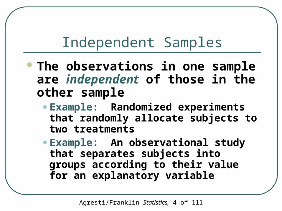
Independent Samples
The observations in one sample are independent of those in the other sample• Example: Randomized experiments that
randomly allocate subjects to two treatments
• Example: An observational study that separates subjects into groups according to their value for an explanatory variable
Agresti/Franklin Statistics, 5 of 111
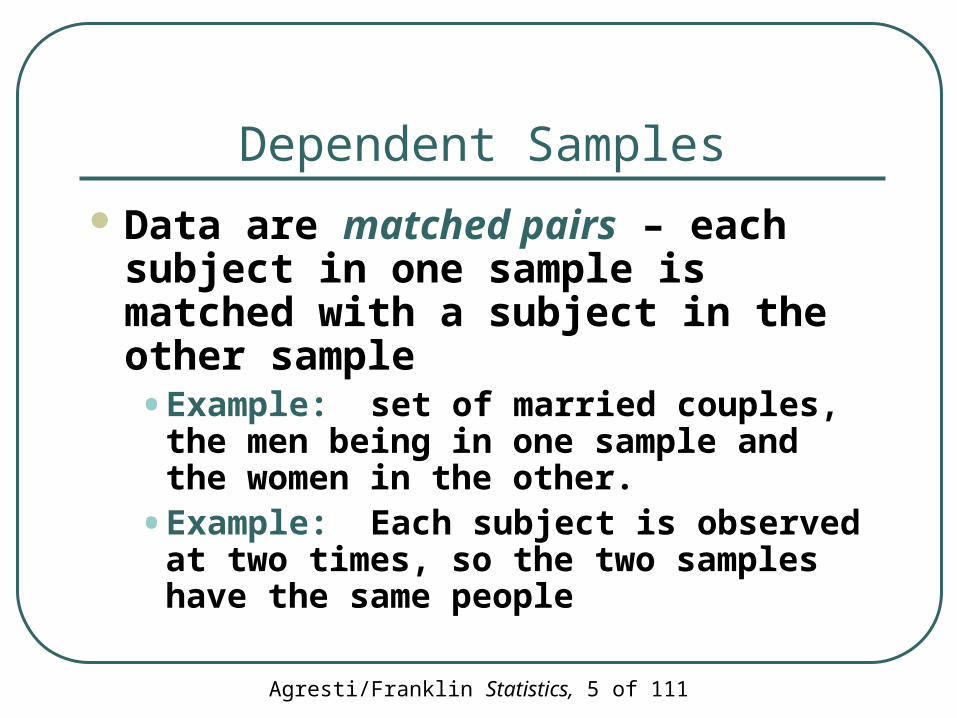
Dependent Samples
Data are matched pairs – each subject in one sample is matched with a subject in the other sample• Example: set of married couples, the men
being in one sample and the women in the other.
• Example: Each subject is observed at two times, so the two samples have the same people

Agresti/Franklin Statistics, 6 of 111
Section 9.1
Categorical Response: How Can We Compare Two Proportions?
Agresti/Franklin Statistics, 7 of 111
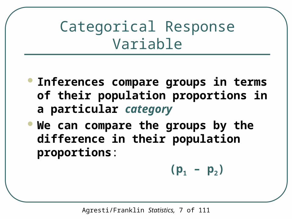
Categorical Response Variable
Inferences compare groups in terms of their population proportions in a particular category
We can compare the groups by the difference in their population proportions:
(p1 – p2)

Agresti/Franklin Statistics, 8 of 111
Example: Aspirin, the Wonder Drug
Recent Titles of Newspaper Articles:
• “Aspirin cuts deaths after heart attack”
• “Aspirin could lower risk of ovarian cancer”
• “New study finds a daily aspirin lowers the risk of colon cancer”
• “Aspirin may lower the risk of Hodgkin’s”

Agresti/Franklin Statistics, 9 of 111
Example: Aspirin, the Wonder Drug
The Physicians Health Study Research Group at Harvard Medical School
• Five year randomized study
• Does regular aspirin intake reduce deaths from heart disease?
Agresti/Franklin Statistics, 10 of 111
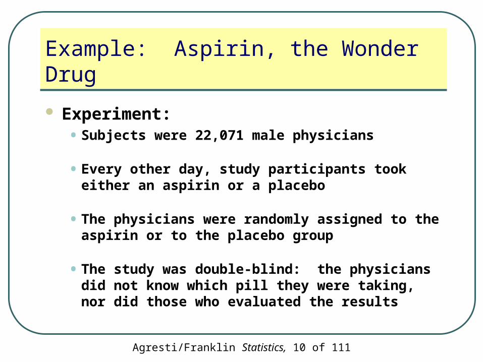
Example: Aspirin, the Wonder Drug
Experiment:• Subjects were 22,071 male physicians
• Every other day, study participants took either an aspirin or a placebo
• The physicians were randomly assigned to the aspirin or to the placebo group
• The study was double-blind: the physicians did not know which pill they were taking, nor did those who evaluated the results

Agresti/Franklin Statistics, 11 of 111
Example: Aspirin, the Wonder Drug
Results displayed in a contingency table:
Agresti/Franklin Statistics, 12 of 111
Example: Aspirin, the Wonder Drug
What is the response variable?
What are the groups to compare?

Agresti/Franklin Statistics, 13 of 111
Example: Aspirin, the Wonder Drug
The response variable is whether the subject had a heart attack, with categories ‘yes’ or ‘no’
The groups to compare are:
• Group 1: Physicians who took a placebo
• Group 2: Physicians who took aspirin

Agresti/Franklin Statistics, 14 of 111
Example: Aspirin, the Wonder Drug
Estimate the difference between the two population parameters of interest
Agresti/Franklin Statistics, 15 of 111
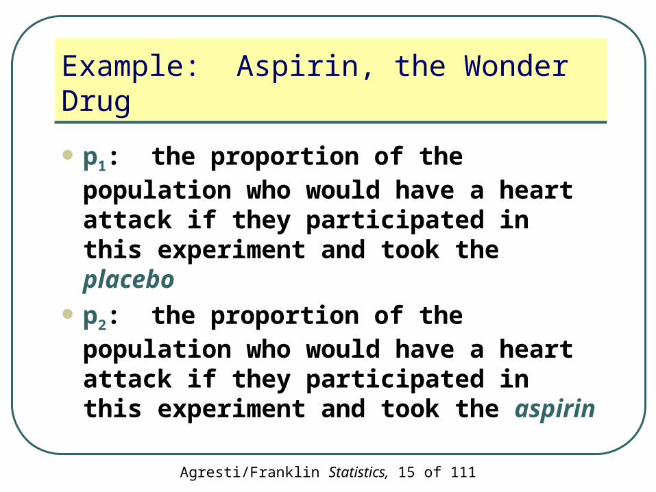
Example: Aspirin, the Wonder Drug
p1: the proportion of the population who would have a heart attack if they participated in this experiment and took the placebo
p2: the proportion of the population who would have a heart attack if they participated in this experiment and took the aspirin
Agresti/Franklin Statistics, 16 of 111
Example: Aspirin, the Wonder Drug
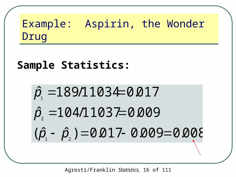
008.0009.0017.0)ˆˆ(
009.011037/104ˆ
017.011034/189ˆ
21
2
1
pp
p
p
Sample Statistics:

Agresti/Franklin Statistics, 17 of 111
Example: Aspirin, the Wonder Drug
To make an inference about the difference of population proportions, (p1 – p2), we need to learn about the variability of the sampling distribution of:
)ˆˆ(21pp
Agresti/Franklin Statistics, 18 of 111
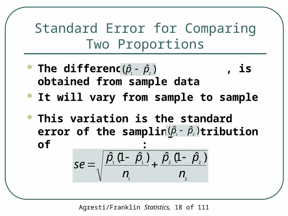
Standard Error for Comparing Two Proportions
The difference, , is obtained from sample data
It will vary from sample to sample
This variation is the standard error of the sampling distribution of :
)ˆˆ(21pp
)ˆˆ(21pp
2
22
1
11)ˆ1(ˆ)ˆ1(ˆ
n
pp
n
ppse
Agresti/Franklin Statistics, 19 of 111
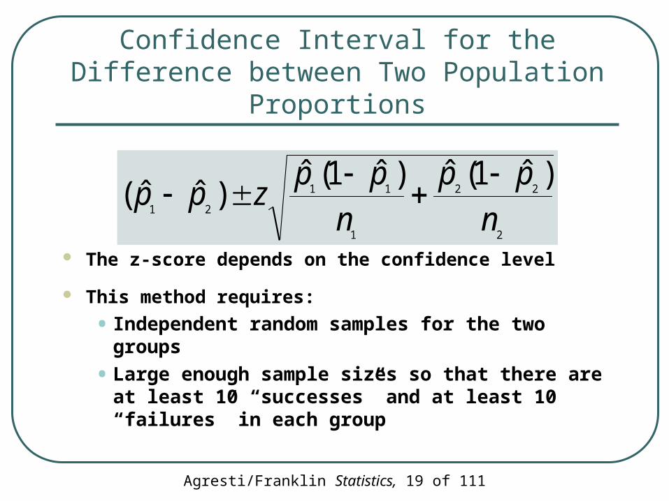
Confidence Interval for the Difference between Two Population Proportions
The z-score depends on the confidence level
This method requires:
• Independent random samples for the two groups
• Large enough sample sizes so that there are at least 10 “successes” and at least 10 “failures” in each group
2
22
1
11
21
)ˆ1(ˆ)ˆ1(ˆ)ˆˆ(
n
pp
n
ppzpp
Agresti/Franklin Statistics, 20 of 111
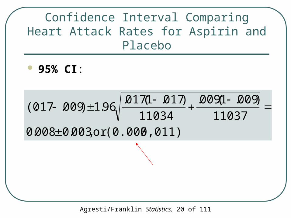
Confidence Interval Comparing Heart Attack Rates for Aspirin and Placebo
95% CI:
0.011) (0.005,or ,003.0008.011037
)009.1(009.
11034
)017.1(017.96.1)009.017(.
Agresti/Franklin Statistics, 21 of 111
Confidence Interval Comparing Heart Attack Rates for Aspirin and Placebo
Since both endpoints of the confidence interval (0.005, 0.011) for (p1- p2) are positive, we infer that (p1- p2) is positive
Conclusion: The population proportion of heart attacks is larger when subjects take the placebo than when they take aspirin

Agresti/Franklin Statistics, 22 of 111
Confidence Interval Comparing Heart Attack Rates for Aspirin and Placebo
The population difference (0.005, 0.011) is small
Even though it is a small difference, it may be important in public health terms
For example, a decrease of 0.01 over a 5 year period in the proportion of people suffering heart attacks would mean 2 million fewer people having heart attacks
Agresti/Franklin Statistics, 23 of 111
Confidence Interval Comparing Heart Attack Rates for Aspirin and Placebo
The study used male doctors in the U.S• The inference applies to the U.S.
population of male doctors
Before concluding that aspirin benefits a larger population, we’d want to see results of studies with more diverse groups
Agresti/Franklin Statistics, 24 of 111
Interpreting a Confidence Interval for a Difference of Proportions
Check whether 0 falls in the CI If so, it is plausible that the population
proportions are equal If all values in the CI for (p1- p2) are
positive, you can infer that (p1- p2) >0 If all values in the CI for (p1- p2) are
negative, you can infer that (p1- p2) <0 Which group is labeled ‘1’ and which is
labeled ‘2’ is arbitrary

Agresti/Franklin Statistics, 25 of 111
Interpreting a Confidence Interval for a Difference of Proportions
The magnitude of values in the confidence interval tells you how large any true difference is
If all values in the confidence interval are near 0, the true difference may be relatively small in practical terms

Agresti/Franklin Statistics, 26 of 111
Significance Tests Comparing Population Proportions
1. Assumptions:
Categorical response variable for two groups
Independent random samples
Agresti/Franklin Statistics, 27 of 111
Significance Tests Comparing Population Proportions
Assumptions (continued):
Significance tests comparing proportions use the sample size guideline from confidence intervals: Each sample should have at least about 10 “successes” and 10 “failures”
Two–sided tests are robust against violations of this condition
• At least 5 “successes” and 5 “failures” is adequate
Agresti/Franklin Statistics, 28 of 111
Significance Tests Comparing Population Proportions
2. Hypotheses: The null hypothesis is the hypothesis of
no difference or no effect:
H0: (p1- p2) =0
• Under the presumption that p1= p2, we create a pooled estimate of the common value of p1and p2
• This pooled estimate is p̂
Agresti/Franklin Statistics, 29 of 111
Significance Tests Comparing Population Proportions
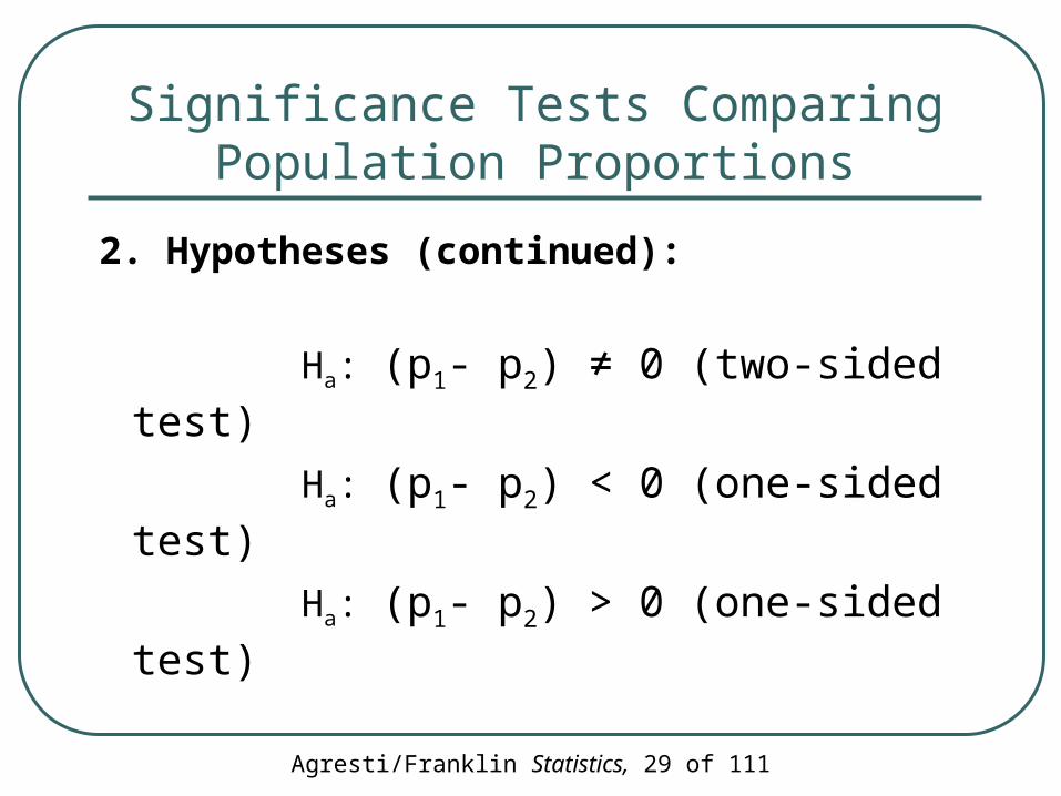
2. Hypotheses (continued):
Ha: (p1- p2) ≠ 0 (two-sided test)
Ha: (p1- p2) < 0 (one-sided test)
Ha: (p1- p2) > 0 (one-sided test)
Agresti/Franklin Statistics, 30 of 111
Significance Tests Comparing Population Proportions
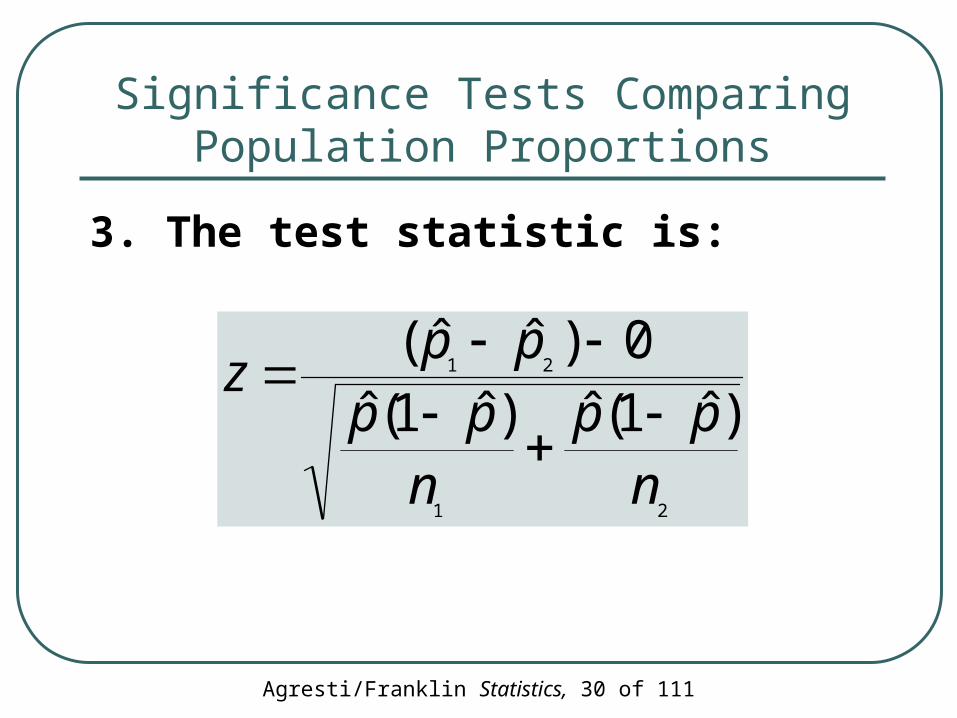
3. The test statistic is:
21
21
)ˆ1(ˆ)ˆ1(ˆ0)ˆˆ(
npp
npppp
z
Agresti/Franklin Statistics, 31 of 111
Significance Tests Comparing Population Proportions
4. P-value: Probability obtained from the standard normal table
5. Conclusion: Smaller P-values give stronger evidence against H0 and supporting Ha
Agresti/Franklin Statistics, 32 of 111
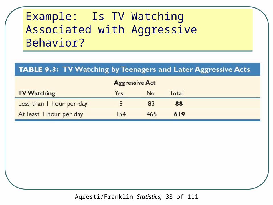
Example: Is TV Watching Associated with Aggressive Behavior?
Various studies have examined a link between TV violence and aggressive behavior by those who watch a lot of TV
A study sampled 707 families in two counties in New York state and made follow-up observations over 17 years
The data shows levels of TV watching along with incidents of aggressive acts
Agresti/Franklin Statistics, 33 of 111
Example: Is TV Watching Associated with Aggressive Behavior?

Agresti/Franklin Statistics, 34 of 111
Example: Is TV Watching Associated with Aggressive Behavior?
Test the Hypotheses:
H0: (p1- p2) = 0
Ha: (p1- p2) ≠ 0
• Using a significance level of 0.05• Group 1: less than 1 hr. of TV per day
• Group 2: at least 1 hr. of TV per day

Agresti/Franklin Statistics, 35 of 111
Example: Is TV Watching Associated with Aggressive Behavior?
Agresti/Franklin Statistics, 36 of 111
Example: Is TV Watching Associated with Aggressive Behavior?
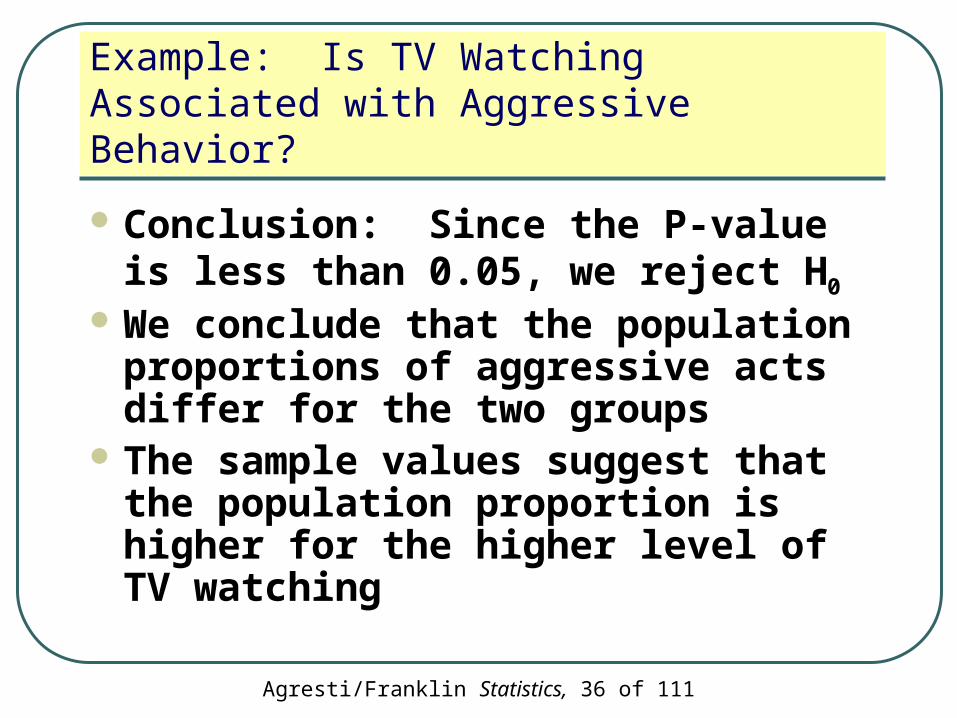
Conclusion: Since the P-value is less than 0.05, we reject H0
We conclude that the population proportions of aggressive acts differ for the two groups
The sample values suggest that the population proportion is higher for the higher level of TV watching

Agresti/Franklin Statistics, 37 of 111
In 2002, the median net worth was estimated as $89,000 for white households and $6000 for black households.
What is the response variable?
a. Net worth
b. Households: white or black
Agresti/Franklin Statistics, 38 of 111
In 2002, the median net worth was estimated as $89,000 for white households and $6000 for black households.
What is the explanatory variable?
a. Net worth
b. Households: white or black

Agresti/Franklin Statistics, 39 of 111
In 2002, the median net worth was estimated as $89,000 for white households and $6000 for black households.
Identify the two groups that are the categories of the explanatory variable.
a. White and Black householdsb. Net worth and households
Agresti/Franklin Statistics, 40 of 111
The estimated medians were based on a sample of households. Were the samples of white households and black households independent samples or dependent samples?
a. Independent samplesb. Dependent samples
In 2002, the median net worth was estimated as $89,000 for white households and $6000 for black households.

Agresti/Franklin Statistics, 41 of 111
Section 9.2
Quantitative Response: How Can We Compare Two Means?
Agresti/Franklin Statistics, 42 of 111
Comparing Means
We can compare two groups on a quantitative response variable by comparing their means
Agresti/Franklin Statistics, 43 of 111
Example: Teenagers Hooked on Nicotine
A 30-month study:
• Evaluated the degree of addiction that teenagers form to nicotine
• 332 students who had used nicotine were evaluated
• The response variable was constructed using a questionnaire called the Hooked on Nicotine Checklist (HONC)

Agresti/Franklin Statistics, 44 of 111
Example: Teenagers Hooked on Nicotine
The HONC score is the total number of questions to which a student answered “yes” during the study
The higher the score, the more hooked on nicotine a student is judged to be
Agresti/Franklin Statistics, 45 of 111
Example: Teenagers Hooked on Nicotine
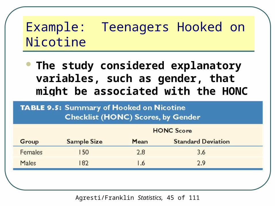
The study considered explanatory variables, such as gender, that might be associated with the HONC score
Agresti/Franklin Statistics, 46 of 111
Example: Teenagers Hooked on Nicotine
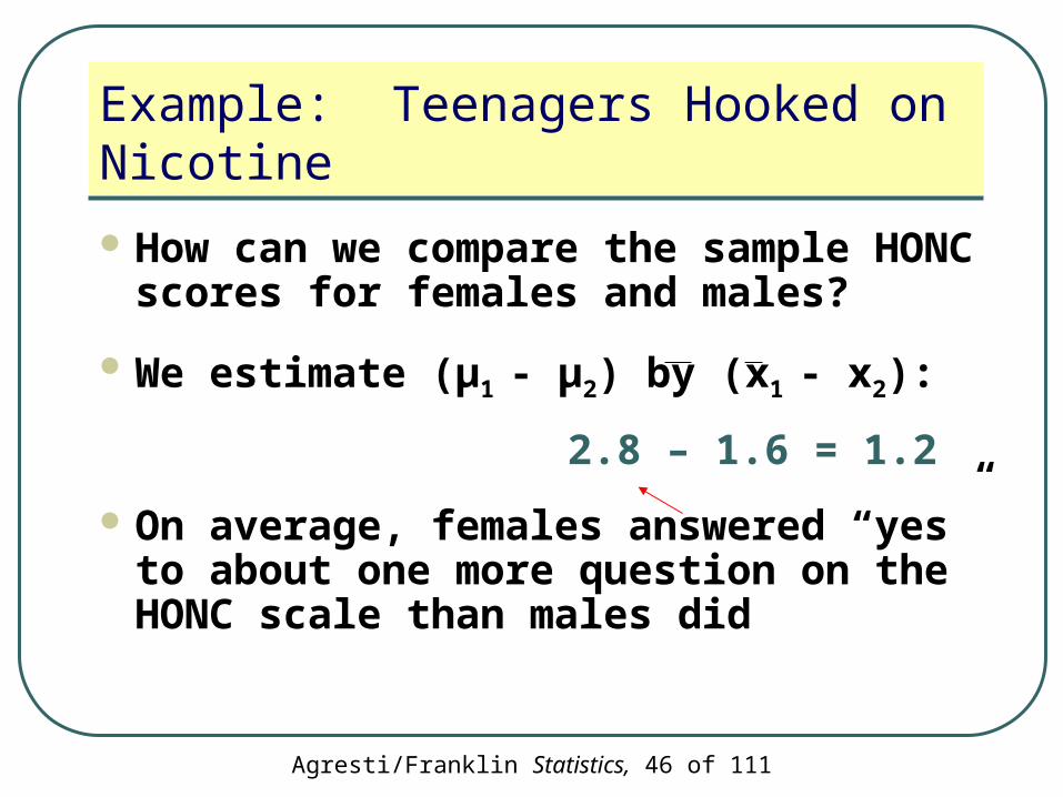
How can we compare the sample HONC scores for females and males?
We estimate (µ1 - µ2) by (x1 - x2):
2.8 – 1.6 = 1.2
On average, females answered “yes” to about one more question on the HONC scale than males did
Agresti/Franklin Statistics, 47 of 111
Example: Teenagers Hooked on Nicotine
To make an inference about the difference between population means, (µ1 – µ2), we need to learn about the variability of the sampling distribution of:
)(21xx
Agresti/Franklin Statistics, 48 of 111
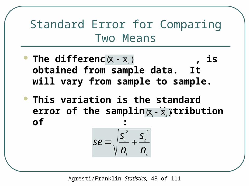
Standard Error for Comparing Two Means
The difference, , is obtained from sample data. It will vary from sample to sample.
This variation is the standard error of the sampling distribution of :
)xx(21
)xx(21
2
2
2
1
2
1
n
s
n
sse
Agresti/Franklin Statistics, 49 of 111
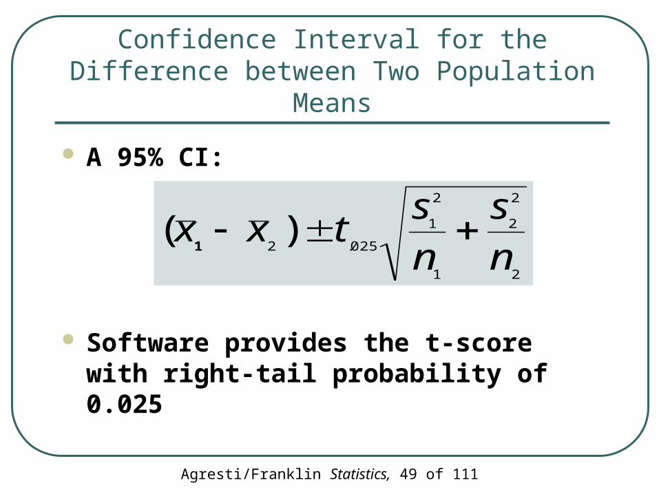
Confidence Interval for the Difference between Two Population Means
A 95% CI:
Software provides the t-score with right-tail probability of 0.025
2
2
2
1
2
1
025.2)(
n
s
n
stxx
1
Agresti/Franklin Statistics, 50 of 111
Confidence Interval for the Difference between Two Population Means
This method assumes:
• Independent random samples from the two groups
• An approximately normal population distribution for each group• this is mainly important for small sample sizes,
and even then the method is robust to violations of this assumption

Agresti/Franklin Statistics, 51 of 111
Example: Nicotine – How Much More Addicted Are Smokers than Ex-Smokers?
Data as summarized by HONC scores for the two groups:
Smokers: x1 = 5.9, s1 = 3.3, n1 = 75
Ex-smokers:x2 = 1.0, s2 = 2.3, n2 = 257
Agresti/Franklin Statistics, 52 of 111
Example: Nicotine – How Much More Addicted Are Smokers than Ex-Smokers?
Were the sample data for the two groups approximately normal?
Most likely not for Group 2 (based on the sample statistics): x2 = 1.0, s2 = 2.3)
Since the sample sizes are large, this lack of normality is not a problem
Agresti/Franklin Statistics, 53 of 111
Example: Nicotine – How Much More Addicted Are Smokers than Ex-Smokers?
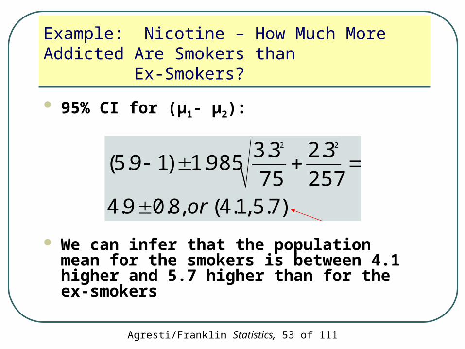
95% CI for (µ1- µ2):
We can infer that the population mean for the smokers is between 4.1 higher and 5.7 higher than for the ex-smokers
)7.5 ,1.4( ,8.09.4257
3.2
75
3.3985.1)19.5(
22
or

Agresti/Franklin Statistics, 54 of 111
How Can We Interpret a Confidence Interval for a Difference of Means?
Check whether 0 falls in the interval When it does, 0 is a plausible value for (µ1 –
µ2), meaning that it is possible that µ1 = µ2
A confidence interval for (µ1 – µ2) that contains only positive numbers suggests that (µ1 – µ2) is positive
We then infer that µ1 is larger than µ2

Agresti/Franklin Statistics, 55 of 111
How Can We Interpret a Confidence Interval for a Difference of Means?
A confidence interval for (µ1 – µ2) that contains only negative numbers suggests that (µ1 – µ2) is negative
We then infer that µ1 is smaller than µ2
Which group is labeled ‘1’ and which is labeled ‘2’ is arbitrary
Agresti/Franklin Statistics, 56 of 111
Significance Tests Comparing Population Means
1. Assumptions:
• Quantitative response variable for two groups
• Independent random samples
Agresti/Franklin Statistics, 57 of 111
Significance Tests Comparing Population Means
Assumptions (continued):
Approximately normal population distributions for each group• This is mainly important for small sample sizes,
and even then the two-sided test is robust to violations of this assumption
Agresti/Franklin Statistics, 58 of 111
Significance Tests Comparing Population Means
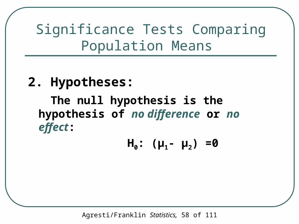
2. Hypotheses:
The null hypothesis is the hypothesis of no difference or no effect:
H0: (µ1- µ2) =0
Agresti/Franklin Statistics, 59 of 111
Significance Tests Comparing Population Proportions
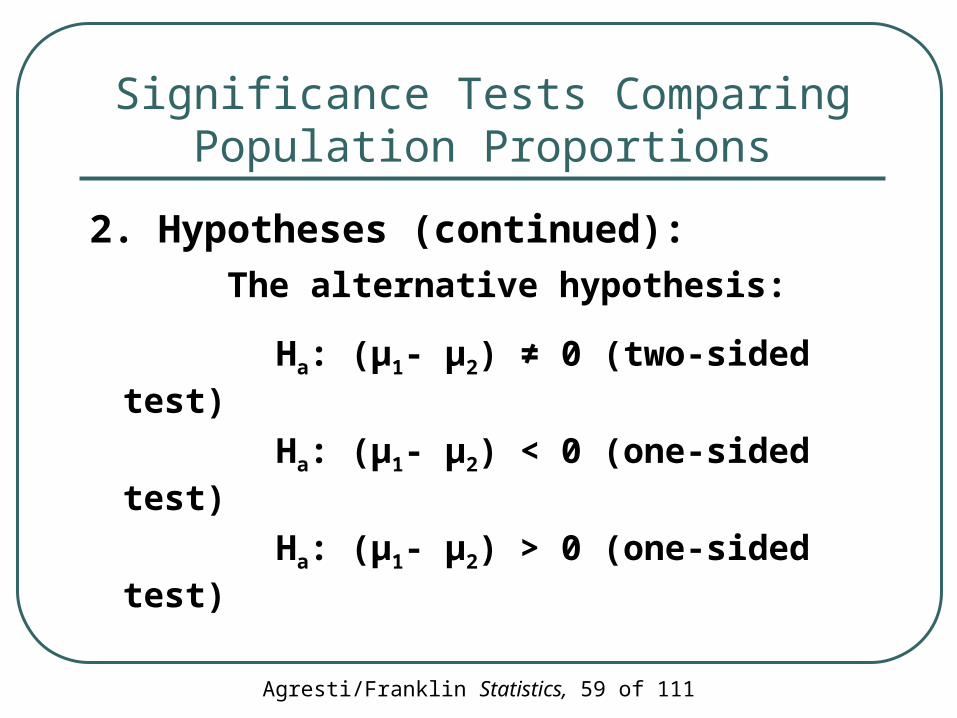
2. Hypotheses (continued):
The alternative hypothesis:
Ha: (µ1- µ2) ≠ 0 (two-sided test)
Ha: (µ1- µ2) < 0 (one-sided test)
Ha: (µ1- µ2) > 0 (one-sided test)
Agresti/Franklin Statistics, 60 of 111
Significance Tests Comparing Population Means
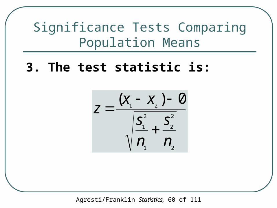
3. The test statistic is:
2
2
2
1
2
1
210)(
ns
nsxx
z
Agresti/Franklin Statistics, 61 of 111
Significance Tests Comparing Population Means
4. P-value: Probability obtained from the standard normal table
5. Conclusion: Smaller P-values give stronger evidence against H0 and supporting Ha
Agresti/Franklin Statistics, 62 of 111
Example: Does Cell Phone Use While Driving Impair Reaction Times?
Experiment:
• 64 college students
• 32 were randomly assigned to the cell phone group
• 32 to the control group
Agresti/Franklin Statistics, 63 of 111
Example: Does Cell Phone Use While Driving Impair Reaction Times?
Experiment (continued):• Students used a machine that simulated
driving situations
• At irregular periods a target flashed red or green
• Participants were instructed to press a “brake button” as soon as possible when they detected a red light

Agresti/Franklin Statistics, 64 of 111
Example: Does Cell Phone Use While Driving Impair Reaction Times?
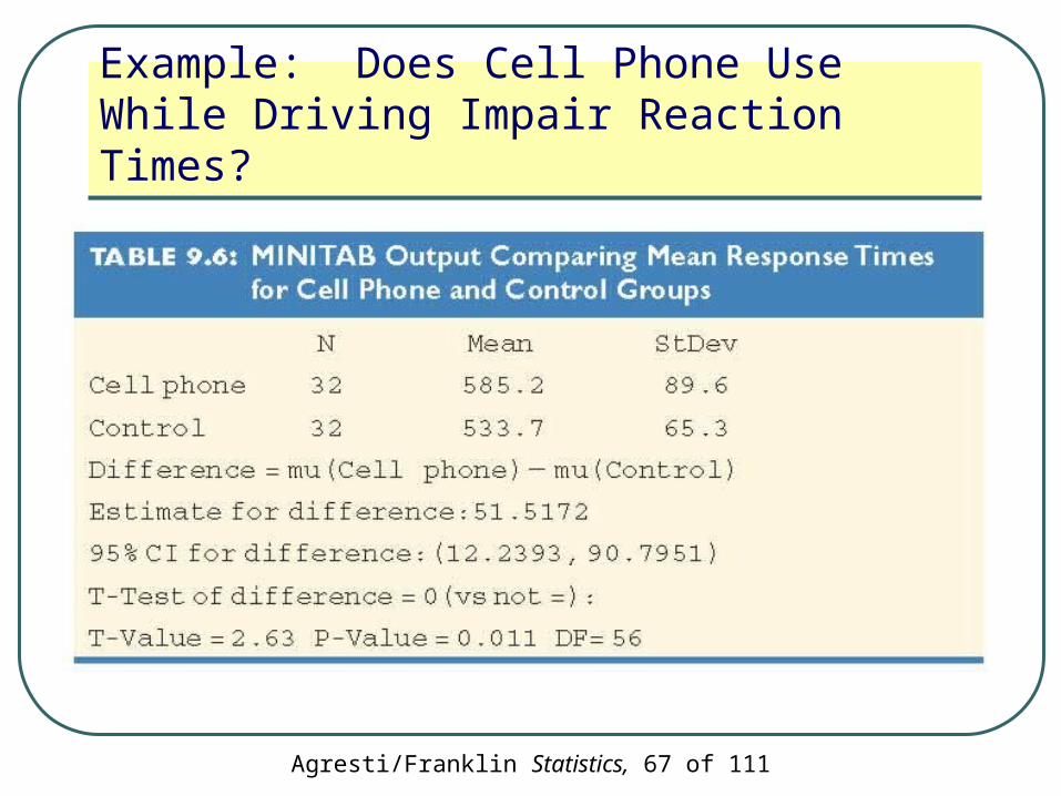
For each subject, the experiment analyzed their mean response time over all the trials
Averaged over all trials and subjects, the mean response time for the cell-phone group was 585.2 milliseconds
The mean response time for the control group was 533.7 milliseconds

Agresti/Franklin Statistics, 65 of 111
Example: Does Cell Phone Use While Driving Impair Reaction Times?
Data:

Agresti/Franklin Statistics, 66 of 111
Example: Does Cell Phone Use While Driving Impair Reaction Times?
Test the hypotheses:
H0: (µ1- µ2) =0
vs.
Ha: (µ1- µ2) ≠ 0
• using a significance level of 0.05
Agresti/Franklin Statistics, 67 of 111
Example: Does Cell Phone Use While Driving Impair Reaction Times?
Agresti/Franklin Statistics, 68 of 111
Example: Does Cell Phone Use While Driving Impair Reaction Times?
Conclusion:• The P-value is less than 0.05, so we can
reject H0
• There is enough evidence to conclude that the population mean response times differ between the cell phone and control groups
• The sample means suggest that the population mean is higher for the cell phone group
Agresti/Franklin Statistics, 69 of 111
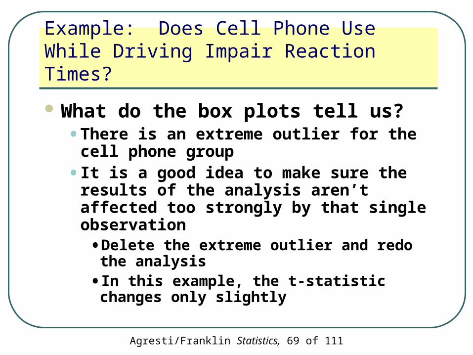
Example: Does Cell Phone Use While Driving Impair Reaction Times?
What do the box plots tell us?• There is an extreme outlier for the cell
phone group
• It is a good idea to make sure the results of the analysis aren’t affected too strongly by that single observation• Delete the extreme outlier and redo the
analysis
• In this example, the t-statistic changes only slightly

Agresti/Franklin Statistics, 70 of 111
Example: Does Cell Phone Use While Driving Impair Reaction Times?
Insight: • In practice, you should not delete outliers
from a data set without sufficient cause (i.e., if it seems the observation was incorrectly recorded)
• It is however, a good idea to check for sensitivity of an analysis to an outlier
• If the results change much, it means that the inference including the outlier is on shaky ground
Agresti/Franklin Statistics, 71 of 111
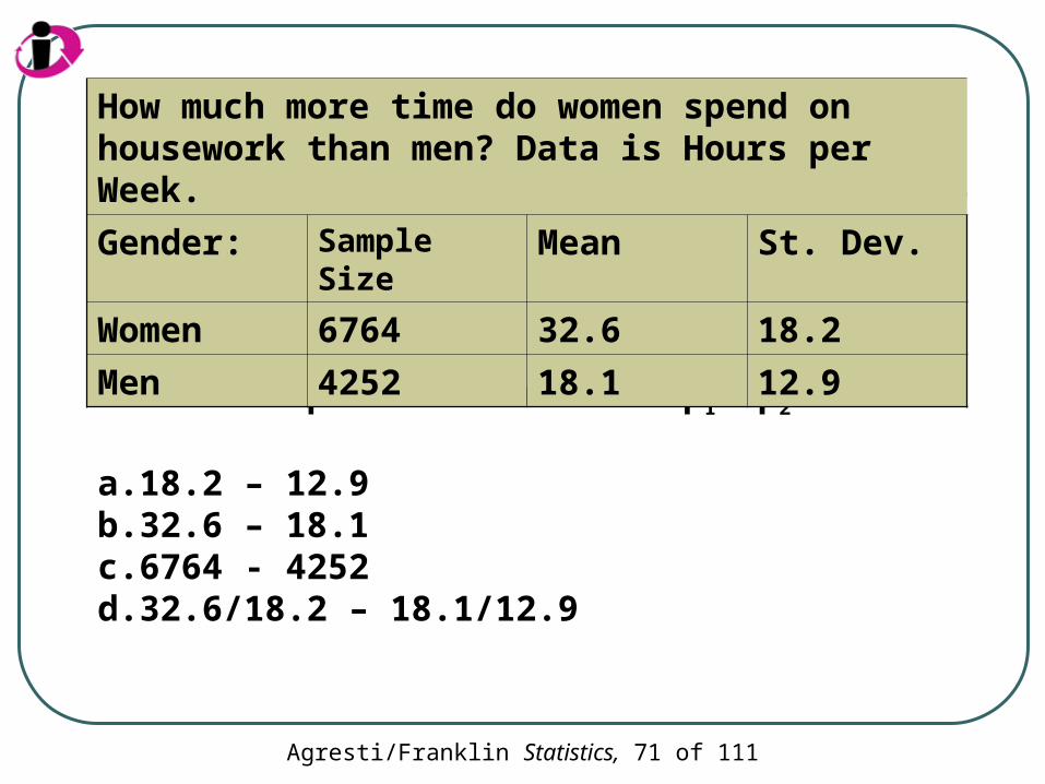
What is a point estimate of µ1- µ2?
a. 18.2 – 12.9b. 32.6 – 18.1c. 6764 - 4252d. 32.6/18.2 – 18.1/12.9
How much more time do women spend on housework than men? Data is Hours per Week.
Gender: Sample Size Mean St. Dev.
Women 6764 32.6 18.2
Men 4252 18.1 12.9
Agresti/Franklin Statistics, 72 of 111
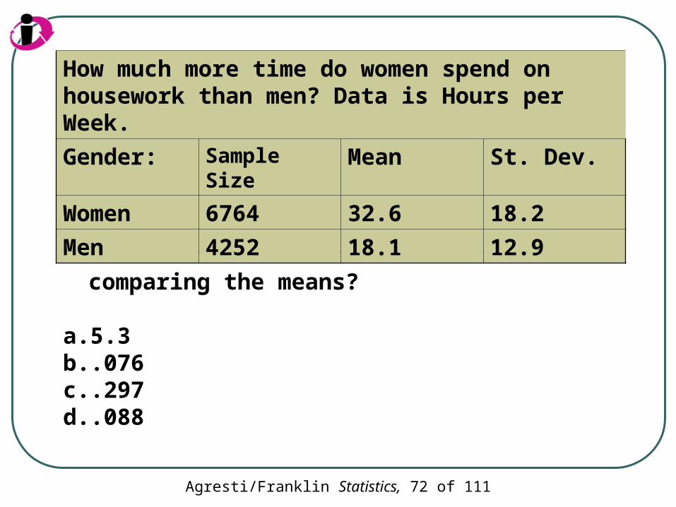
What is the standard error for comparing the means?
a. 5.3b. .076c. .297d. .088
How much more time do women spend on housework than men? Data is Hours per Week.
Gender: Sample Size Mean St. Dev.
Women 6764 32.6 18.2
Men 4252 18.1 12.9

Agresti/Franklin Statistics, 73 of 111
What factor causes the standard error to be small compared to the sample standard deviations for the two groups?
a. sample meansb. sample standard deviationsc. sample sizesd. genders
How much more time do women spend on housework than men? Data is Hours per Week.
Gender: Sample Size Mean St. Dev.
Women 6764 32.6 18.2
Men 4252 18.1 12.9
Agresti/Franklin Statistics, 74 of 111
Section 9.3
Other Ways of Comparing Means and Comparing Proportions
Agresti/Franklin Statistics, 75 of 111
Alternative Method for Comparing Means
An alternative t- method can be used when, under the null hypothesis, it is reasonable to expect the variability as well as the mean to be the same
This method requires the assumption that the population standard deviations be equal

Agresti/Franklin Statistics, 76 of 111
The Pooled Standard Deviation
This alternative method estimates the common value σ of σ1 and σ1 by:
2
)1()1(
21
2
22
2
11
nn
snsns
Agresti/Franklin Statistics, 77 of 111
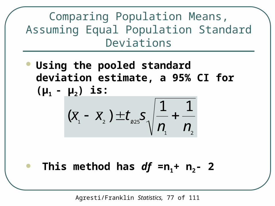
Comparing Population Means, Assuming Equal Population Standard Deviations
Using the pooled standard deviation estimate, a 95% CI for (µ1 - µ2) is:
This method has df =n1+ n2- 2
21
025.21
11)(
nnstxx

Agresti/Franklin Statistics, 78 of 111
Comparing Population Means, Assuming Equal Population Standard Deviations
The test statistic for H0: µ1=µ2 is:
This method has df =n1+ n2- 2
21
21
11)(
nns
xxt
Agresti/Franklin Statistics, 79 of 111
Comparing Population Means, Assuming Equal Population Standard Deviations
These methods assume:
• Independent random samples from the two groups
• An approximately normal population distribution for each group• This is mainly important for small sample sizes,
and even then, the CI and the two-sided test are usually robust to violations of this assumption
• σ1=σ2
Agresti/Franklin Statistics, 80 of 111
The Ratio of Proportions: The Relative Risk
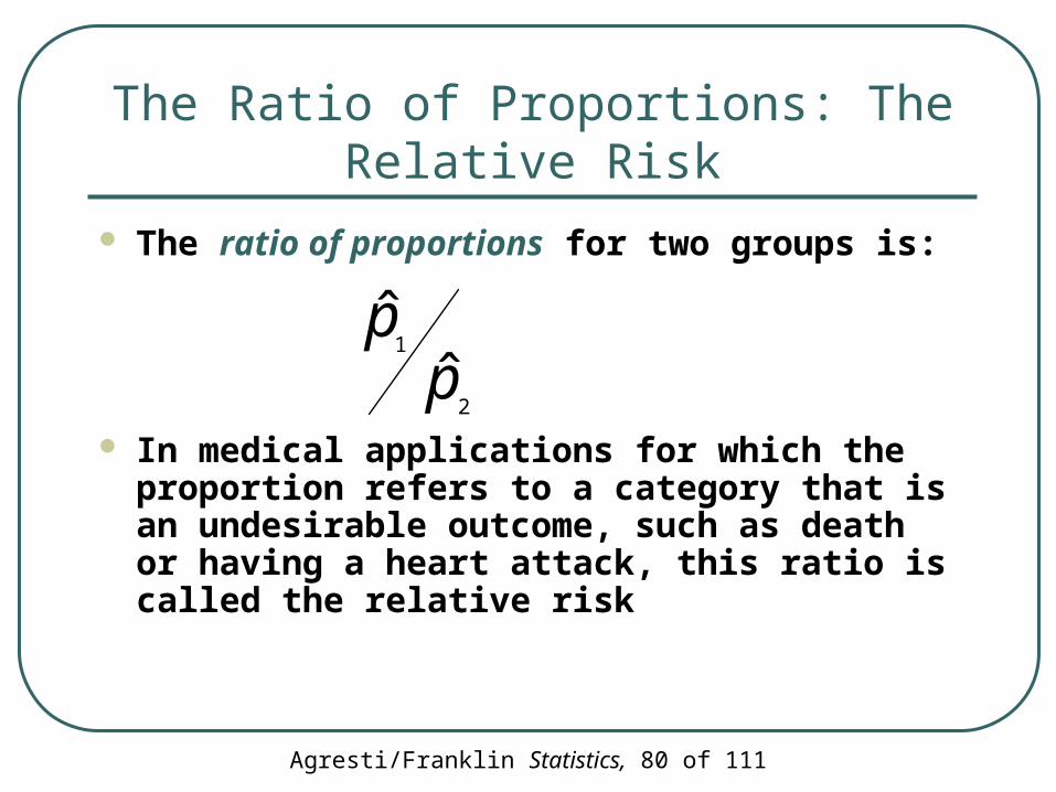
The ratio of proportions for two groups is:
In medical applications for which the proportion refers to a category that is an undesirable outcome, such as death or having a heart attack, this ratio is called the relative risk
2
1
ˆˆp
p
Agresti/Franklin Statistics, 81 of 111
Section 9.4
How Can We Analyze Dependent Samples?

Agresti/Franklin Statistics, 82 of 111
Dependent Samples
Each observation in one sample has a matched observation in the other sample
The observations are called matched pairs

Agresti/Franklin Statistics, 83 of 111
Example: Matched Pairs Design for Cell Phones and Driving Study
The cell phone analysis presented earlier in this text used independent samples:
• One group used cell phones
• A separate control group did not use cell phones

Agresti/Franklin Statistics, 84 of 111
Example: Matched Pairs Design for Cell Phones and Driving Study
An alternative design used the same subjects for both groups
• Reaction times are measured when subjects performed the driving task without using cell phones and then again while using cell phones
Agresti/Franklin Statistics, 85 of 111
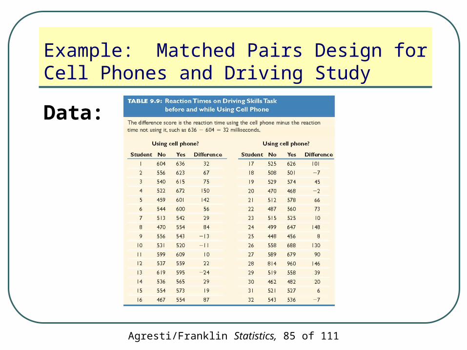
Example: Matched Pairs Design for Cell Phones and Driving Study
Data:
Agresti/Franklin Statistics, 86 of 111
Example: Matched Pairs Design for Cell Phones and Driving Study
Benefits of using dependent samples (matched pairs):• Many sources of potential bias are
controlled so we can make a more accurate comparison
• Using matched pairs keeps many other factors fixed that could affect the analysis
• Often this results in the benefit of smaller standard errors
Agresti/Franklin Statistics, 87 of 111
Example: Matched Pairs Design for Cell Phones and Driving Study
To Compare Means with Matched Pairs, Use Paired Differences:
• For each matched pair, construct a difference score
• d = (reaction time using cell phone) – (reaction time without cell phone)
• Calculate the sample mean of these differences: xd
Agresti/Franklin Statistics, 88 of 111
For Dependent Samples (Matched Pairs)
Mean of Differences
=
Difference of Means
Agresti/Franklin Statistics, 89 of 111
For Dependent Samples (Matched Pairs)
The difference (x1 – x2) between the means of the two samples equals the mean xd of the difference scores for the matched pairs
The difference (µ1 – µ2) between the population means is identical to the parameter µd that is the population mean of the difference scores

Agresti/Franklin Statistics, 90 of 111
For Dependent Samples (Matched Pairs)
Let n denote the number of observations in each sample
This equals the number of difference scores The 95 % CI for the population mean difference
is:
deviation standard their is s
sdifference theofmean sample theis
d
025.
d
dd
xn
stx

Agresti/Franklin Statistics, 91 of 111
For Dependent Samples (Matched Pairs)
To test the hypothesis H0: µ1 = µ2 of equal means, we can conduct the single-sample test of H0: µd = 0 with the difference scores
The test statistic is:
1 with 0 ndf
nsx
td
d
Agresti/Franklin Statistics, 92 of 111
For Dependent Samples (Matched Pairs)
These paired-difference inferences are special cases of single-sample inferences about a population mean so they make the same assumptions
Agresti/Franklin Statistics, 93 of 111
Paired-difference Inferences
Assumptions:• The sample of difference scores is a
random sample from a population of such difference scores
• The difference scores have a population distribution that is approximately normal• This is mainly important for small samples
(less than about 30) and for one-sided inferences
Agresti/Franklin Statistics, 94 of 111
Paired-difference Inferences
Confidence intervals and two-sided tests are robust: They work quite well even if the normality assumption is violated
One-sided tests do not work well when the sample size is small and the distribution of differences is highly skewed
Agresti/Franklin Statistics, 95 of 111
Example: Matched Pairs Analysis for Cell Phones and Driving Study
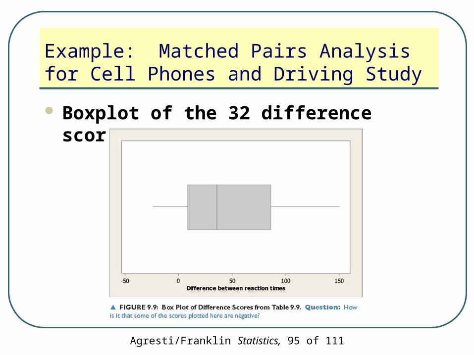
Boxplot of the 32 difference scores

Agresti/Franklin Statistics, 96 of 111
Example: Matched Pairs Analysis for Cell Phones and Driving Study
The box plot shows skew to the right for the difference scores• Two-sided inference is robust to violations
of the assumption of normality
The box plot does not show any severe outliers
Agresti/Franklin Statistics, 97 of 111
Example: Matched Pairs Analysis for Cell Phones and Driving Study
Agresti/Franklin Statistics, 98 of 111
Example: Matched Pairs Analysis for Cell Phones and Driving Study
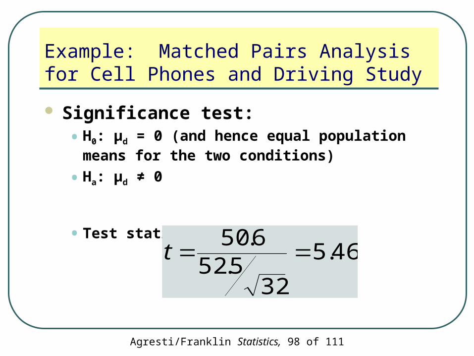
Significance test:• H0: µd = 0 (and hence equal population means for
the two conditions)
• Ha: µd ≠ 0
• Test statistic:
46.5
325.52
6.50 t

Agresti/Franklin Statistics, 99 of 111
Example: Matched Pairs Analysis for Cell Phones and Driving Study
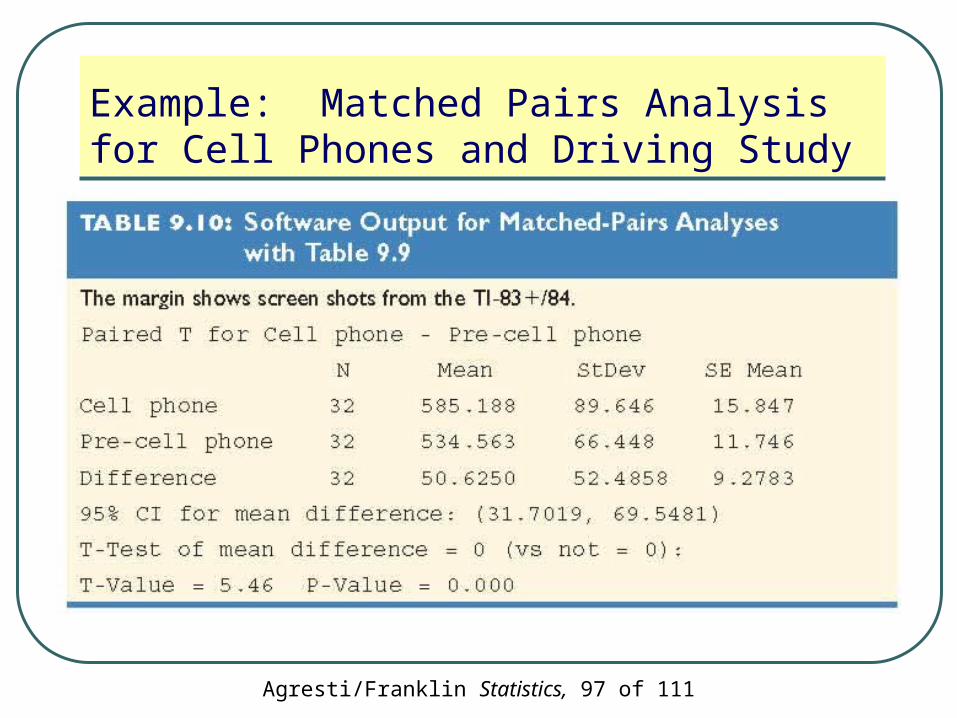
The P-value displayed in the output is 0.000
There is extremely strong evidence that the population mean reaction times are different

Agresti/Franklin Statistics, 100 of 111
Example: Matched Pairs Analysis for Cell Phones and Driving Study
95% CI for µd =(µ1 - µ2):
69.5) (31.7,or
18.950.6 )32
5.52(040.26.50
Agresti/Franklin Statistics, 101 of 111
Example: Matched Pairs Analysis for Cell Phones and Driving Study
We infer that the population mean when using cell phones is between about 32 and 70 milliseconds higher than when not using cell phones
The confidence interval is more informative than the significance test, since it predicts just how large the difference must be

Agresti/Franklin Statistics, 102 of 111
Section 9.5
How Can We Adjust for Effects of Other Variables?

Agresti/Franklin Statistics, 103 of 111
A Practically Significant Difference
When we find a practically significant difference between two groups, can we identify a reason for the difference?
Warning: An association may be due to a lurking variable not measured in the study
Agresti/Franklin Statistics, 104 of 111
Example: Is TV Watching Associated with Aggressive Behavior?
In a previous example, we saw that teenagers who watch more TV have a tendency later in life to commit more aggressive acts
Could there be a lurking variable that influences this association?

Agresti/Franklin Statistics, 105 of 111
Example: Is TV Watching Associated with Aggressive Behavior?
Perhaps teenagers who watch more TV tend to attain lower educational levels and perhaps lower education tends to be associated with higher levels of aggression
Agresti/Franklin Statistics, 106 of 111
Example: Is TV Watching Associated with Aggressive Behavior?
We need to measure potential lurking variables and use them in the statistical analysis
If we thought that education was a potential lurking variable we would what to measure it
Agresti/Franklin Statistics, 107 of 111
Example: Is TV Watching Associated with Aggressive Behavior?
Agresti/Franklin Statistics, 108 of 111
Example: Is TV Watching Associated with Aggressive Behavior?
This analysis uses three variables:
• Response variable: Whether the subject has committed aggressive acts
• Explanatory variable: Level of TV watching
• Control variable: Educational level
Agresti/Franklin Statistics, 109 of 111
Control Variable
A control variable is a variable that is held constant in a multivariate analysis (more than two variables)

Agresti/Franklin Statistics, 110 of 111
Can An Association Be Explained by a Third Variable?
Treat the third variable as a control variable
Conduct the ordinary bivariate analysis while holding that control variable constant at fixed values
Whatever association occurs cannot be due to effect of the control variable
Agresti/Franklin Statistics, 111 of 111
Example: Is TV Watching Associated with Aggressive Behavior?
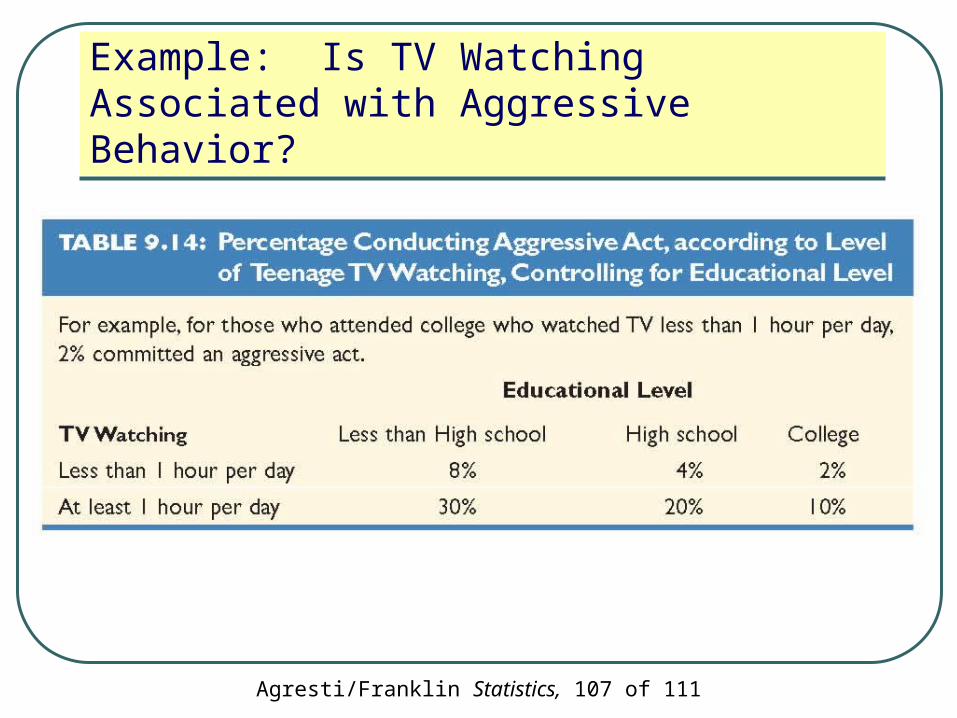
At each educational level, the percentage committing an aggressive act is higher for those who watched more TV
For this hypothetical data, the association observed between TV watching and aggressive acts was not because of education
Recommended