An introduction and basic quantities of interest
Actuarial mathematics 1Lecture 1. Introduction.
Edward Furman
Department of Mathematics and StatisticsYork University
September 15, 2010
Edward Furman Actuarial mathematics MATH 3280 1 / 11
An introduction and basic quantities of interest
Introduction.
Would people spend same money today if there were noretirement programs, life insurance contracts or socialsecurity systems?
Edward Furman Actuarial mathematics MATH 3280 2 / 11
An introduction and basic quantities of interest
Introduction.
Would people spend same money today if there were noretirement programs, life insurance contracts or socialsecurity systems?
Definition 1.1 (Insurance.)
An insurance is a mechanism for reducing the adverse financialimpact of random events that prevent the fulfillment ofreasonable expectations (see, Bowers et al., 1997).
Definition 1.2 (Insurance.)
Insurance is an equitable transfer of a risk of a monetary lossfrom an insured to an insurer in exchange for premium(s) (weshall use this one).
Insurance is thus a hedge against financial contingent losses.
Edward Furman Actuarial mathematics MATH 3280 2 / 11
An introduction and basic quantities of interest
Keywords.
Risk – Possibility of financial loss.
Edward Furman Actuarial mathematics MATH 3280 3 / 11
An introduction and basic quantities of interest
Keywords.
Risk – Possibility of financial loss.
Loss – Monetary units equivalent amount of damagesuffered by the insured(s).
Edward Furman Actuarial mathematics MATH 3280 3 / 11
An introduction and basic quantities of interest
Keywords.
Risk – Possibility of financial loss.
Loss – Monetary units equivalent amount of damagesuffered by the insured(s).
Insured or policyholder – an entity that purchases aninsurance. It can be a person, a company, even an insurer.
Insurer – a seller of insurance.
Premium – the amount to be charged for an insurance. Itcan be a single payment or not.
We shall not distinguish between the so - called loss andpayment events, though these two can be quite different.
Where does the maths come into all these?
Edward Furman Actuarial mathematics MATH 3280 3 / 11
An introduction and basic quantities of interest
Introductory example.
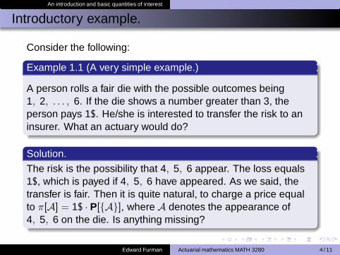
Consider the following:
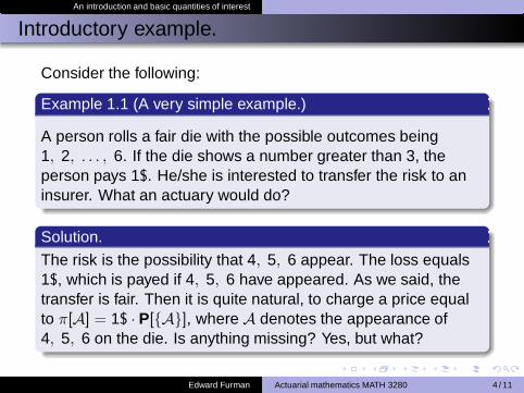
Example 1.1 (A very simple example.)
A person rolls a fair die with the possible outcomes being1, 2, . . . , 6. If the die shows a number greater than 3, theperson pays 1$. He/she is interested to transfer the risk to aninsurer. What an actuary would do?
Solution.
The risk is
Edward Furman Actuarial mathematics MATH 3280 4 / 11
An introduction and basic quantities of interest
Introductory example.
Consider the following:
Example 1.1 (A very simple example.)
A person rolls a fair die with the possible outcomes being1, 2, . . . , 6. If the die shows a number greater than 3, theperson pays 1$. He/she is interested to transfer the risk to aninsurer. What an actuary would do?
Solution.
The risk is the possibility that 4, 5, 6 appear. The loss equals
Edward Furman Actuarial mathematics MATH 3280 4 / 11
An introduction and basic quantities of interest
Introductory example.
Consider the following:
Example 1.1 (A very simple example.)
A person rolls a fair die with the possible outcomes being1, 2, . . . , 6. If the die shows a number greater than 3, theperson pays 1$. He/she is interested to transfer the risk to aninsurer. What an actuary would do?
Solution.
The risk is the possibility that 4, 5, 6 appear. The loss equals1$, which is payed if 4, 5, 6 have appeared. As we said, thetransfer is fair. Then it is quite natural, to charge a price equalto
Edward Furman Actuarial mathematics MATH 3280 4 / 11
An introduction and basic quantities of interest
Introductory example.
Consider the following:
Example 1.1 (A very simple example.)
A person rolls a fair die with the possible outcomes being1, 2, . . . , 6. If the die shows a number greater than 3, theperson pays 1$. He/she is interested to transfer the risk to aninsurer. What an actuary would do?
Solution.
The risk is the possibility that 4, 5, 6 appear. The loss equals1$, which is payed if 4, 5, 6 have appeared. As we said, thetransfer is fair. Then it is quite natural, to charge a price equalto π[A] = 1$ · P[A], where A denotes the appearance of4, 5, 6 on the die. Is anything missing?
Edward Furman Actuarial mathematics MATH 3280 4 / 11
An introduction and basic quantities of interest
Introductory example.
Consider the following:
Example 1.1 (A very simple example.)
A person rolls a fair die with the possible outcomes being1, 2, . . . , 6. If the die shows a number greater than 3, theperson pays 1$. He/she is interested to transfer the risk to aninsurer. What an actuary would do?
Solution.
The risk is the possibility that 4, 5, 6 appear. The loss equals1$, which is payed if 4, 5, 6 have appeared. As we said, thetransfer is fair. Then it is quite natural, to charge a price equalto π[A] = 1$ · P[A], where A denotes the appearance of4, 5, 6 on the die. Is anything missing? Yes, but what?
Edward Furman Actuarial mathematics MATH 3280 4 / 11
An introduction and basic quantities of interest
The value of 1$ changes with time, so a discounting should bedone. We neglect that discounting for a while. What is theprobability of interest?
Edward Furman Actuarial mathematics MATH 3280 5 / 11
An introduction and basic quantities of interest
The value of 1$ changes with time, so a discounting should bedone. We neglect that discounting for a while. What is theprobability of interest? We know that P : F → [0, 1], where F is
Edward Furman Actuarial mathematics MATH 3280 5 / 11
An introduction and basic quantities of interest
The value of 1$ changes with time, so a discounting should bedone. We neglect that discounting for a while. What is theprobability of interest? We know that P : F → [0, 1], where F isthe sigma - algebra over a space of elementary outcomes, i.e.,over Ω. In our simple example, we readily have that
Edward Furman Actuarial mathematics MATH 3280 5 / 11
An introduction and basic quantities of interest
The value of 1$ changes with time, so a discounting should bedone. We neglect that discounting for a while. What is theprobability of interest? We know that P : F → [0, 1], where F isthe sigma - algebra over a space of elementary outcomes, i.e.,over Ω. In our simple example, we readily have that 2Ω = 1, 2, 3, 4, 5, 6. Then because P is countably additive,we have that P[ω ∈ Ω : ω > 3] = P[4 ∪ 5 ∪ 6] = 1/2.The price our actuary would come with is then
π[A] = 1$ · 0.5 = 0.5$,
which is the premium the insured would be required to pay. Youexpected it, didn’t you?
Edward Furman Actuarial mathematics MATH 3280 5 / 11

An introduction and basic quantities of interest
Very often, the sample space is much more cumbersome thanthe one we have just mentioned. Think of, e.g.,
Edward Furman Actuarial mathematics MATH 3280 6 / 11
An introduction and basic quantities of interest
Very often, the sample space is much more cumbersome thanthe one we have just mentioned. Think of, e.g.,
Choosing a real number in [0, 1]. Ω = r ∈ R : 0 ≤ r ≤ 1,
which has an uncountable number of elementary events, andsimilarly, but more related to our course,
An age of death of a new born child.Ω = r ∈ R+ : 0 < r ≤ 123.
Edward Furman Actuarial mathematics MATH 3280 6 / 11

An introduction and basic quantities of interest
Very often, the sample space is much more cumbersome thanthe one we have just mentioned. Think of, e.g.,
Choosing a real number in [0, 1]. Ω = r ∈ R : 0 ≤ r ≤ 1,
which has an uncountable number of elementary events, andsimilarly, but more related to our course,
An age of death of a new born child.Ω = r ∈ R+ : 0 < r ≤ 123.
Ages of death of a couple.Ω = r = (r1, r2)
′ ∈ R2+ : 0 < r1, r2 ≤ 123.
Edward Furman Actuarial mathematics MATH 3280 6 / 11
An introduction and basic quantities of interest
Very often, the sample space is much more cumbersome thanthe one we have just mentioned. Think of, e.g.,
Choosing a real number in [0, 1]. Ω = r ∈ R : 0 ≤ r ≤ 1,
which has an uncountable number of elementary events, andsimilarly, but more related to our course,
An age of death of a new born child.Ω = r ∈ R+ : 0 < r ≤ 123.
Ages of death of a couple.Ω = r = (r1, r2)
′ ∈ R2+ : 0 < r1, r2 ≤ 123.
Minimum of two ages of death.Ω = r ∈ R+ : 0 < r ≤ 123.
Severity of an insurance loss. Ω = r ∈ R+.
Frequency of an insurance loss. Ω = n ∈ N.
How would our actuary determine the probability for any one ofthe above being equal to a specific value? And then the price?Let’s go back to Example 1.1.
Edward Furman Actuarial mathematics MATH 3280 6 / 11
An introduction and basic quantities of interest
Solution of Example 1.1 (cont.)
Let’s define a function X : Ω → R, such that X (A) = 1 andX (Ac) = 0.
Edward Furman Actuarial mathematics MATH 3280 7 / 11
An introduction and basic quantities of interest
Solution of Example 1.1 (cont.)
Let’s define a function X : Ω → R, such that X (A) = 1 andX (Ac) = 0.The domain is
Edward Furman Actuarial mathematics MATH 3280 7 / 11
An introduction and basic quantities of interest
Solution of Example 1.1 (cont.)
Let’s define a function X : Ω → R, such that X (A) = 1 andX (Ac) = 0.The domain is in the sample space, and the range isbinary, so it’s actually an indicator random variable (r.v.). Theprobability that the person pays 1$ is then
Edward Furman Actuarial mathematics MATH 3280 7 / 11

An introduction and basic quantities of interest
Solution of Example 1.1 (cont.)
Let’s define a function X : Ω → R, such that X (A) = 1 andX (Ac) = 0.The domain is in the sample space, and the range isbinary, so it’s actually an indicator random variable (r.v.). Theprobability that the person pays 1$ is then
P[ω ∈ Ω : X (ω) = 1] =
Edward Furman Actuarial mathematics MATH 3280 7 / 11
An introduction and basic quantities of interest
Solution of Example 1.1 (cont.)
Let’s define a function X : Ω → R, such that X (A) = 1 andX (Ac) = 0.The domain is in the sample space, and the range isbinary, so it’s actually an indicator random variable (r.v.). Theprobability that the person pays 1$ is then
P[ω ∈ Ω : X (ω) = 1] = P[X (ω) = 1]
Edward Furman Actuarial mathematics MATH 3280 7 / 11

An introduction and basic quantities of interest
Solution of Example 1.1 (cont.)
Let’s define a function X : Ω → R, such that X (A) = 1 andX (Ac) = 0.The domain is in the sample space, and the range isbinary, so it’s actually an indicator random variable (r.v.). Theprobability that the person pays 1$ is then
P[ω ∈ Ω : X (ω) = 1] = P[X (ω) = 1] = P[X = 1] =
Edward Furman Actuarial mathematics MATH 3280 7 / 11
An introduction and basic quantities of interest
Solution of Example 1.1 (cont.)
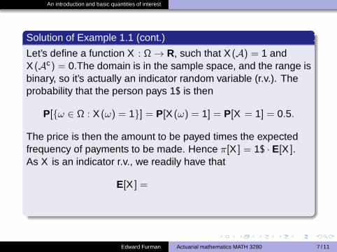
Let’s define a function X : Ω → R, such that X (A) = 1 andX (Ac) = 0.The domain is in the sample space, and the range isbinary, so it’s actually an indicator random variable (r.v.). Theprobability that the person pays 1$ is then
P[ω ∈ Ω : X (ω) = 1] = P[X (ω) = 1] = P[X = 1] = 0.5.
The price is then the amount to be payed times the expectedfrequency of payments to be made. Hence π[X ] = 1$ · E[X ].As X is an indicator r.v., we readily have that
E[X ] =
Edward Furman Actuarial mathematics MATH 3280 7 / 11
An introduction and basic quantities of interest
Solution of Example 1.1 (cont.)
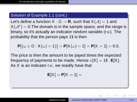
Let’s define a function X : Ω → R, such that X (A) = 1 andX (Ac) = 0.The domain is in the sample space, and the range isbinary, so it’s actually an indicator random variable (r.v.). Theprobability that the person pays 1$ is then
P[ω ∈ Ω : X (ω) = 1] = P[X (ω) = 1] = P[X = 1] = 0.5.
The price is then the amount to be payed times the expectedfrequency of payments to be made. Hence π[X ] = 1$ · E[X ].As X is an indicator r.v., we readily have that
E[X ] = P[X = 1] =
Edward Furman Actuarial mathematics MATH 3280 7 / 11
An introduction and basic quantities of interest
Solution of Example 1.1 (cont.)
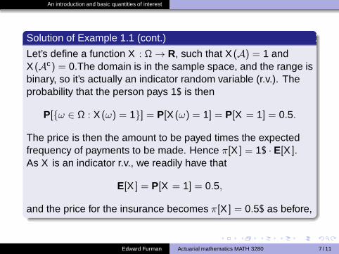
Let’s define a function X : Ω → R, such that X (A) = 1 andX (Ac) = 0.The domain is in the sample space, and the range isbinary, so it’s actually an indicator random variable (r.v.). Theprobability that the person pays 1$ is then
P[ω ∈ Ω : X (ω) = 1] = P[X (ω) = 1] = P[X = 1] = 0.5.
The price is then the amount to be payed times the expectedfrequency of payments to be made. Hence π[X ] = 1$ · E[X ].As X is an indicator r.v., we readily have that
E[X ] = P[X = 1] = 0.5,
and the price for the insurance becomes π[X ] = 0.5$ as before,
Edward Furman Actuarial mathematics MATH 3280 7 / 11
An introduction and basic quantities of interest
At home.
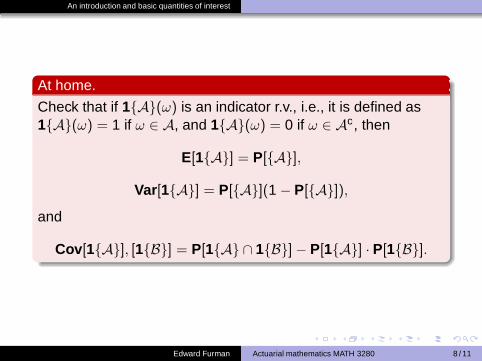
Check that if 1A(ω) is an indicator r.v., i.e., it is defined as1A(ω) = 1 if ω ∈ A, and 1A(ω) = 0 if ω ∈ Ac, then
E[1A] = P[A],
Var[1A] = P[A](1 − P[A]),
and
Cov[1A], [1B] = P[1A ∩ 1B]− P[1A] · P[1B].
Edward Furman Actuarial mathematics MATH 3280 8 / 11
An introduction and basic quantities of interest
Example 1.1 (cont.)
To conclude the example, we shall augment it with the timevalue of money. To this end, let v = (1+ i)−1 be the discountingfactor. Thus the present value (p.v.) of 1$ payed at time 1is
Edward Furman Actuarial mathematics MATH 3280 9 / 11
An introduction and basic quantities of interest
Example 1.1 (cont.)
To conclude the example, we shall augment it with the timevalue of money. To this end, let v = (1+ i)−1 be the discountingfactor. Thus the present value (p.v.) of 1$ payed at time 1is1$ · v . Therefore if we assume that the person gets his/herone dollar at time 1, the premium becomesπ[X ] = v · E[X ] = 0.5v . Can it anyhow be extended to arandom time of the payment?Let’s say that the time of payment is represented by the r.v. Yindependent of X . The premium, that our actuary would nowcharge, is
π[X ] = E[X · vY ]
We shall call present values a la 1$ · vY , actuarial presentvalues (a.p.v.). This completes Example 1.
The premium is nothing else but the a.p.v. of the losses.
Edward Furman Actuarial mathematics MATH 3280 9 / 11
An introduction and basic quantities of interest
Example 1.2
A couple wishes to insure the life of its new born child. Whatwould an actuary do to compute the premium for the contract ifthe insurance amount of 10,000$ is repayed upon child’s death,and the interest rate is fixed to i throughout?
Solution.
If the length of child’s life (=time of his/her death) is describedby the continuous r.v. T (0) : Ω → A ⊂ R+, withΩ = t ∈ R+ : 0 < t ≤ 123, then the price to be payed is
Edward Furman Actuarial mathematics MATH 3280 10 / 11
An introduction and basic quantities of interest
Example 1.2
A couple wishes to insure the life of its new born child. Whatwould an actuary do to compute the premium for the contract ifthe insurance amount of 10,000$ is repayed upon child’s death,and the interest rate is fixed to i throughout?
Solution.
If the length of child’s life (=time of his/her death) is describedby the continuous r.v. T (0) : Ω → A ⊂ R+, withΩ = t ∈ R+ : 0 < t ≤ 123, then the price to be payed is
π[T (0)] = E[10,000 · vT (0)].
End of Example 1.2.
This course will mostly deal with various characteristics ofthe r.v.’s a la T (0).
Edward Furman Actuarial mathematics MATH 3280 10 / 11
An introduction and basic quantities of interest
Key points.
MATH 3280 3.00 F.
We shall in the sequel assume that life times are r.v.’s, andwe shall thus explore:
Various life formations (statuses) and their future life timesas well as sources of their deaths (decrements),
and the corresponding
cumulative and decumulative distribution functions (c.d.f’s)and (d.d.f’s);
probability density functions (p.d.f’s) and the force ofmortality for continuous r.v.’s;
probability mass functions (p.m.f’s) and life tables forcurtuate r.v.’s;
percentiles, expectations, variances, covariances.
Edward Furman Actuarial mathematics MATH 3280 11 / 11
Recommended