Edward Furman - YorkU Math and Statsefurman/actmath2008/lecture2.pdf · Feel comfortable with the deterministic approach to life tables. Edward Furman, Actuarial mathematics MATH3280

Survival distributions and life tablesActuarial mathematics 3280

Department of Mathematics and StatisticsYork University

Edward Furman

[email protected]

Edward Furman, Actuarial mathematics MATH3280 – p. 1/66

Outline

After we have completed this theme you will be able to:

Define survival-time random variables (rv’s) for one life;

Calculate the expected values, variances, probabilitiesand percentiles for survival-time rv’s;

Define the continuous type survival-time rv using a:1. uniform distribution,2. constant force of mortality,3. hyperbolic assumption.

Be able to characterize life tables using the completeexpectation of life, median future lifetime, mode, etc.

Understand and apply the concept of select life tables.

Feel comfortable with the deterministic approach to lifetables.


Survival function

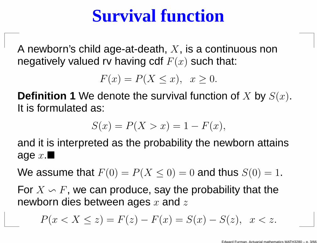
A newborn’s child age-at-death, X, is a continuous nonnegatively valued rv having cdf F (x) such that:

F (x) = P (X ≤ x), x ≥ 0.

Definition 1 We denote the survival function of X by S(x).It is formulated as:

S(x) = P (X > x) = 1 − F (x),

and it is interpreted as the probability the newborn attainsage x.

We assume that F (0) = P (X ≤ 0) = 0 and thus S(0) = 1.

For X v F , we can produce, say the probability that thenewborn dies between ages x and z

P (x < X ≤ z) = F (z) − F (x) = S(x) − S(z), x < z.


Time-until death for a person aged x

The probability the newborn will die between ages x and zgiven survival to age x is

P (x < X ≤ z|X > x) =F (z) − F (x)

1 − F (x)=

S(x) − S(z)

S(x).

The future lifetime of (x) that is X − x is denoted by T (x).Thus, the probability that (x) dies between ages x and z is:

P (T (x) ≤ z − x).

Are the two latter equations equivalent?


Example 1 Suppose the cdf of (0) is given byF (t) = t/80, 0 < t ≤ 80 and F (t) = 1 otherwise. What is theprobability that a new born:

1. dies no latter than age 30,

2. survives to age 50,

3. dies after age 30 but not latter than age 50.

Solution(a) P (X ≤ 30) = F (30) = 3/8,(b) P (X > 50) = 1 − F (50) = 1 − 5/8 = 3/8,(c) P (30 < X ≤ 50) = F (50) − F (30) = 1/4.


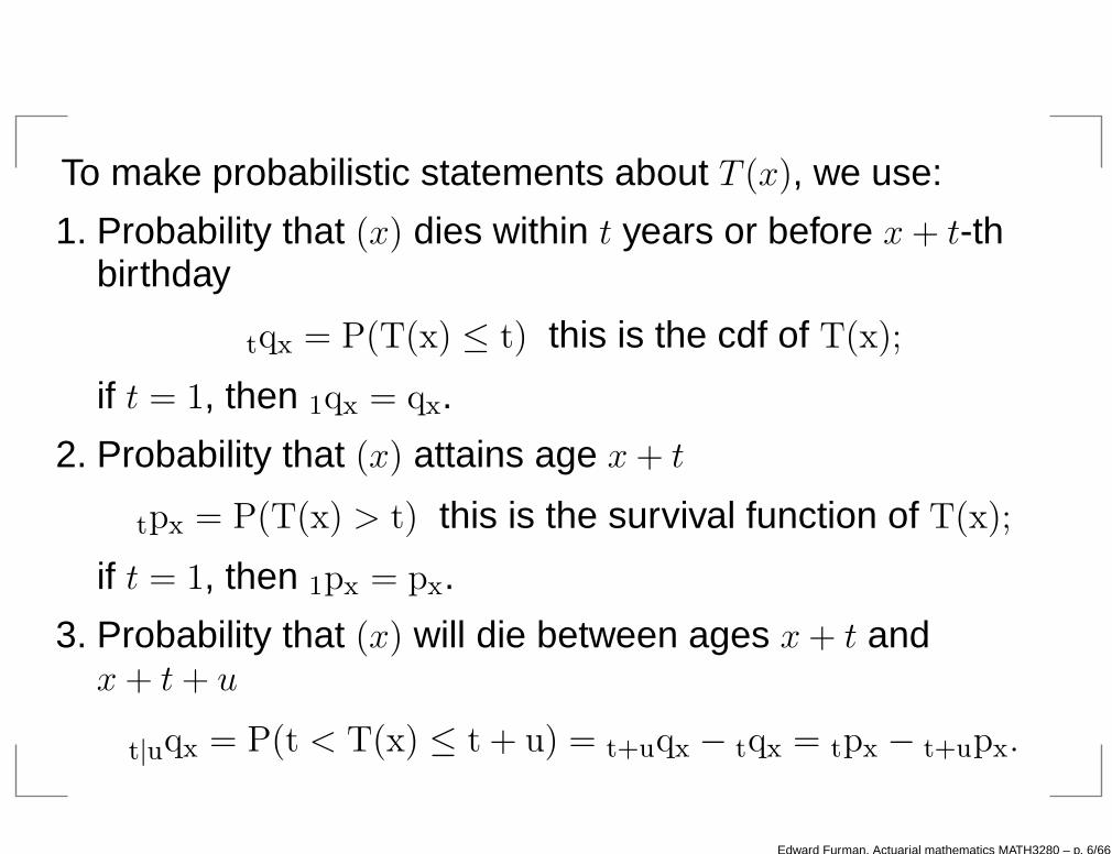
To make probabilistic statements about T (x), we use:

1. Probability that (x) dies within t years or before x + t-thbirthday

tqx = P(T(x) ≤ t) this is the cdf of T(x);

if t = 1, then 1qx = qx.

2. Probability that (x) attains age x + t

tpx = P(T(x) > t) this is the survival function of T(x);

if t = 1, then 1px = px.

3. Probability that (x) will die between ages x + t andx + t + u

t|uqx = P(t < T(x) ≤ t + u) = t+uqx − tqx = tpx − t+upx.


Assumption 1 The observation of survival at age x yieldsthe same conditional distribution of survival as thehypothesis that a new born has survived to age x.Then:

tpx = P (T (x) > t) = P (X > x + t|X > x) =x+tp0

xp0,

tqx = P (T (x) ≤ t) = 1 − P (T (x) > t) =x+tq0 − xq0

xp0.

Also, under Assumption 1, we have that:

t|uqx = tpx · uqx+t.

Proof

t|uqx = P (t < T (x) ≤ t + u) = P (x + t < X ≤ x + t + u|X > x)


Curtate future lifetime

t|uqx =P (X ≤ x + t + u) − P (X ≤ x + t)

P (X > x)

=S(x + t) − S(x + t + u)

S(x)

=S(x + t)

S(x)

S(x + t) − S(x + t + u)

S(x + t),

as needed.

Definition 2 Discrete rv K(x) denotes the number of futureyears completed by (x) prior to death. K(x) is the greatestinteger in T (x) and its pmf is:

P (K(x) = k) = P (k ≤ T (x) < k + 1) = P (k < T (x) ≤ k + 1)

= kpx · 1qx+k = k|1qx.


Note that k|qx is a pmf. Indeed:∞∑

k=0

P (K(x) = k) =∞∑

k=0

k|qx = 1.

The cdf of K(x) is:

P (K(x) ≤ k) =

k∑

h=0

P (K(x) = h) =

k∑

h=0

h|qx

=k∑

h=0

(h+1qx − hqx) = k+1qx − 0qx

= k+1qx.

The cdf of K(x) is thus a step function:

FK(x)(y) = P (K(x) ≤ y) = k+1qx, y ≥ 0,

. Edward Furman, Actuarial mathematics MATH3280 – p. 9/66

and k is the greatest integer in y.

Example 2 Consider the cdf

F (x) =

√

x

100, 0 ≤ x ≤ 100.

What is the probability that a newborn lives at least 25complete years?Solution

P (K(0) ≥ 25) = 1 − P (K(0) < 25) = 1 − P (K(0) ≤ 24)

= 1 − 25q0 = 1 − F(25) = 0.5.


Force of mortality

Recall that the probability the newborn will die betweenages x and x + ∆x given survival to age x is

P (x < X ≤ x + ∆x|X > x) =F (x + ∆x) − F (x)

1 − F (x).

Then, taking lim∆x→0+, we have that:

lim∆x→0+

P (x < X ≤ x + ∆x|X > x) =f(x)∆x

S(x)= µ(x)∆x ≥ 0,

where

µ(x) =f(x)

S(x)=

F ′(x)

S(x)=

−S′(x)

S(x)

is called the force of mortality and for each age x, it givesthe value of the conditional density function of X at exactage x given survival to that age.


The force of mortality can be used to specify the distributionof X.Proof Due to the definition of µ(y), we have that:

µ(y) =−S′(y)

S(y)= −

d

dylog S(y),

which leads to−µ(y)dy = d log S(y).

Integrating the above from x to x + n leads to:

−

∫ x+n

x

µ(y)dy =

∫ x+n

x

d log S(y) = logS(x + n)

S(x)

= log npx.


Taking exponentials:

npx = exp

(

−

∫ x+n

xµ(y)dy

)

,

which after the change of variables s = y − x yields

npx = exp

(

−

∫ n

0µ(x + s)ds

)

.

For a newborn live, i.e. (0)

np0 = exp

(

−

∫ n

0µ(s)ds

)

F (n) = 1 − S(n) = 1 − exp

(

−

∫ n

0µ(s)ds

)

.


Second fundamental theorem

Theorem 1 Let f be a continuous real-valued functiondefined on [a, b]. Let F be the antiderivative of f , i.e.,

f(x) =d

dxF (x)

for every x ∈ [a, b]. Then, we have that:∫ b

a

f(x)dx = F (b) − F (a).

Corollary 1 It follows that for every x ∈ [a, b],

F (x) =

∫ x

a

f(t)dt + F (a),

and thusd

dxF (x) =

d

dx

(∫ x

a

f(t)dt + F (a)

)

= f(x).


Force of mortality - cont.

Back to the force of mortality, we now have that:

F ′(n) = f(n) =d

dn

(

1 − exp

(

−

∫ n

0µ(s)ds

))

= exp

(

−

∫ n

0µ(s)ds

)

µ(n) = np0µ(n).

The pdf of T (x) can be found as follows:

fT (x)(n) =d

dnnqx =

d

dn

(

1 −S(x + n)

S(x)

)

=S(x + n)

S(x)

(

−S′(x + n)

S(x + n)

)

= npxµ(x + n), n ≥ 0.


Thus∫ ∞

0npxµ(x + n)dn = 1.

To summarize (Each row shows 4 ways to express thefunction in the left column.)

F (x) S(x) f(x) µ(x)

F (x) F (x) 1 − S(x)∫ x

0 f(y)dy 1 − e−∫

x

0µ(y)dy

S(x) 1 − F (x) S(x)∫∞x f(y)dy e−

∫

x

0µ(y)dy

f(x) F ′(x) −S′(x) f(x) µ(x)e−∫

x

0µ(y)dy

µ(x) F ′(x)1−F (x)

−S′(x)S(x)

f(x)S(x) µ(x)

At home, make sure you are able to build similar table forT (x).


Example 3 Show that

limn→∞

∫ x+n

x

µ(y)dy = ∞.

Solution Note that:

limn→∞

npx = 0.

Thus:

limn→∞

∫ x+n

x

µ(y)dy = limn→∞

(−lognpx) = ∞,

as needed.

The above example literally says that we have a restrictionon possible force of mortality functions.


Example 4 Let Ac = Ω\A within a sample space andP (Ac 6= 0). The following expresses an identity in probabilitytheory:

P (A ∪ B) = P (A) + P (B ∩ Ac) = P (A) + P (Ac)P (B|Ac).

Rewrite this identity in actuarial notations for the events:A = T (x) ≤ t and B = t < T (x) ≤ 1, 0 < t < 1.Solution

P (A ∪ B) becomes P (T (x) ≤ 1) = qx

P (A) becomes tqx

P (B|Ac) is 1−tqx+t.

At last, we obtain:

qx = tqx + tpx · 1−tqx+t.


To conclude:

Rewrite the expression for P (B ∩ Ac)from Example 4 inactuarial notations.

You have to solve all the exercises on the website andanswer questions on the slides.

ReferencesBowers, N. L., Hickman, J. C., Nesbitt, C. J., Jones, D. A.and Gerber, H. U. (1997). Actuarial mathematics, 2ndedition, Society of Actuaries, Itasca, Illinois.


Life table functions

Denote by l0 a group of newborns (e.g. l0 = 100000). Eachnewborn’s age-at-death has a distribution specified by S(x).Also, let L(x) be the rv denoting the number of survivors toage x, generally indexed by j = 1, 2, . . . , l0. Then:

L(x) =l0∑

j=1

1(j),

where 1(j) is the indicator function for the survival of life jthat is 1(j) = 1 if this life survives to age x and 0 otherwise.

Definition 3 We denote by lx the expected number ofsurvivors to age x from the l0 newborns, and we formulatethis as: (E[1(A)] = P (A))

lx = E[L(x)] = E

l0∑

j=1

1(j)

= l0S(x).


Does the latter expectation remind you an expectationof a well known rv?Note that by general reasoning we have that:

lx = l0S(x)

as well.Let nD(x) = L(x) − L(x + n) be the rv representing thegroup of deaths between ages x and x + n.Definition 4 We denote by ndx the expected number ofdeaths between ages x and x + n among the initial l0 lives:

ndx = E[nD(x)] = l0(S(x) − S(x + n)) = lx − lx+n.

We can express the force of mortality in terms of lx, l0:

µ(x) = −S′(x)

S(x)= −

dlxlxdx

.


We can further easily produce (show at home ):

lx = l0 exp

(

−

∫ x

0µ(y)dy

)

,

lx+n = lx exp

(

−

∫ x+n

x

µ(y)dy

)

,

lx − lx+n =

∫ x+n

x

lyµ(y)dy.

Example 5 Show that the local extreme points of lxµ(x)correspond to points of inflection of lx.Proof Indeed,

d

dxlxµ(x) = −

d

dxlx

dlxlxdx

= −d2

dx2lx.


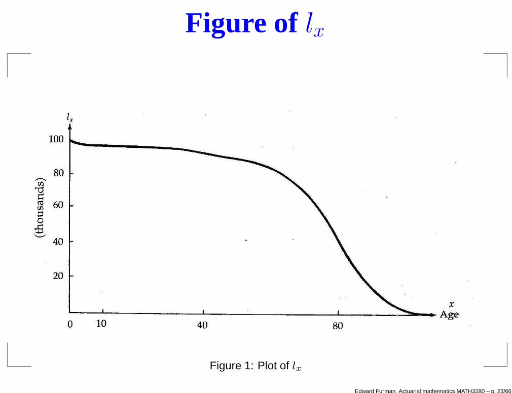
Figure of lx

Figure 1: Plot of lx


Figure of lxµ(x)

Figure 2: Plot of lxµ(x)


Figure of a force of mortality

Figure 3: Plot of µ(x)


Fractional ages

Life table functions investigated hitherto specify the cdf ofK(x) completely. To specify the cdf of (T (x) we mustpostulate an analytic form or adopt an assumption inaddition to the life table functions we had.

We will further review three different assumptions forfractional ages:

1. Linear interpolation,

S(x + t) = (1 − t)S(x) + tS(x + 1).

2. Exponential interpolation,

log S(x + t) = (1 − t) log S(x) + t log S(x + 1).

3. Harmonic interpolation,

1/S(x + t) = (1 − t)/S(x) + t/S(x + 1).


Linear interpolation

Figure 4: Linear interpolation for lx+s, 0 < s < 1


Due to the plot, we can find the value of Lx+s from thefollowing equations:

lx − lx+s

lx − lx+1=

x + s − x

x + 1 − x= s,

which yieldlx+s = lx − slx + slx+1.

Finally, we find that:

lx+s = (1 − s)lx + slx+1.


Linear interpolation:

lx+s = (1 − s)lx + slx+1 = lx − sdx,

where dx = lx − lx+1. Further, dividing by lx, we have that

spx = 1 − sqx ⇒ sqx = sqx.

As qx is tabulated we can calculate sqx for any non-integerduration s.Also, we have that

sqx = P (T (x) ≤ s) =

∫ s

0fT (x)(t)dt =

∫ s

0tpxµx+tdt = s · qx

and thus

fT (x)(s) =d

dssqx = qx, for 0 < s < 1.


As fT (x)(s) is constant in s and equal to qx, deaths are saidto be uniformly distributed over the interval (x, x + 1).We have seen that

µ(x) =f(x)

S(x)=

f(x)

xp0and, similarly, µ(x + s) =

fT (x)(s)

spx.

Then, the force of mortality is

µ(x + s) =qx

spx=

qx

1 − s · qx,

which increases in s.If both the age and the duration are non-integer, i.e., wewant to calculate s−tqx+t, 0 < t < s < 1, then

spx =t px ·s−t px+t ⇒ s−tpx+t =spx

tpx.


Hence,

s−tqx+t = 1 −s−t px+t = 1 −spx

tpx= 1 −

1 −s qx

1 −t qx,

which after applying the UDD assumption reduces to

s−tqx+t = 1 −1 − s · qx

1 − t · qx=

(s − t)qx

1 − t · qx, for 0 < t < s < 1.


Example 6 Given p90 = 0.75, calculate under the UDDassumption 1

12

q90 and 1

12

q90 11

12

.

Solution We have that

1

12

q90 =1

12· q90 =

1

12· (1 − p90) =

1

12· 0.25 = 0.02083.

Also, taking t = 1112 and s = 1, we arrive at

s−tqx+t = 1

12

q90 11

12

=(1 − 11

12)q90

1 − 1112q90

=1120.25

1 − 11120.25

= 0.027027.


Example 7 For two lives aged (x) with independent futurelifetimes k|qx = 0.1(k + 1), k = 0, 1, 2 UDD is assumed. Whatis the probability that both lives will survive 2.25 years.Solution Let us calculate the probability that (x) will survive2.25 years. Let lx = 1, then using dx+k = lx · k|qx, we get

lx+1 = lx − dx = 1 − 0.1 = 0.9;

lx+2 = lx+1 − dx+1 = 0.9 − 0.2 = 0.7;

lx+3 = lx+2 − dx+2 = 0.7 − 0.3 = 0.4.

Linearly interpolating between lx+2 and lx+3, we obtain that

lx+2.25 = (1−0.25)0.7+0.25·0.4 = 0.625,⇒ 2.25px =lx+2.25

lx= 0.625.

As lives are independent the answer is 0.6252.


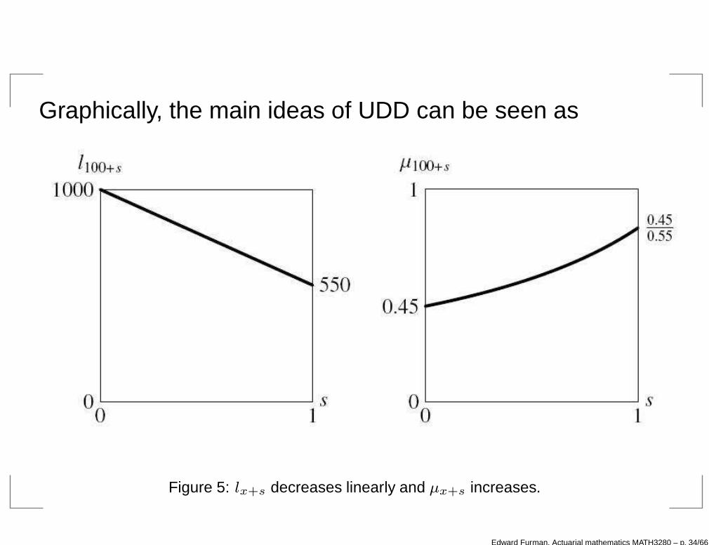
Graphically, the main ideas of UDD can be seen as

Figure 5: lx+s decreases linearly and µx+s increases.


Constant force of mortality - CFM

The force of mortality can be used to specify the distributionof X. Indeed,

µ(x) =−S′(x)

S(x)= −

d

dxlogS(x)

−

∫ x+s

x

µ(y)dy = log

[

S(x + s)

S(x)

]

= logspx

spx = exp

(

−

∫ x+s

x

µ(y)dy

)

or for t = y − x

= exp

(

−

∫ s

0µ(x + t)dt

)

.

Under the CFM assumption, we find the value of µ as

px = exp

(

−

∫ 1

0µ(x + t)dt

)

= exp(−µ) ⇒ µ = −log(px).


Further, for 0 < s < 1, we have that

spx = exp(−sµ) = (px)s.

Also, if both the age and the duration are non-integer, thenfor 0 < t < s < 1, we have that

s−tqx+t = 1 −s−t px+t = 1 − exp

(

−

∫ s

t

µ(x + r)dr

)

= 1 − exp

(

−

∫ s

t

µdr

)

= 1 − exp(−(s − t)µ).

It follows that s−tqx+t =s−t qx. why?

At home show that the CFM is consistent withexponential interpolation.


Example 8 Given p90 = 0.75, calculate under the CFMassumption 1

12

q90 and 1

12

q90 11

12

.

Solution First we find the constant µ over the interval(90,91). Namely,

µ = −log(p90) = −log(0.75) = 0.287682.

Then, we have that

1

12

q90 = 1 − exp(−1

12µ) = 0.023688.

Further, for t = 1112 and s = 1,

1

12

q90 11

12

= 1−exp

(

−

(

1 −11

12

)

µ

)

= 1−exp

(

−1

12µ

)

= 0.023688.


Graphically, the main ideas of CFM can be seen as

Figure 6: lx+s decreases and µx+s is constant.


The Balducci assumption

Hyperbolic interpolation: for 0 < s < 1

1

lx+s=

1 − s

lx+

s

lx+1=

(1 − s)lx+1 + slxlx · lx+1

,

which implies that

lx+s =lx · lx+1

lx+1 + sdx=

lx+1

px + sqx,

and dividing by lx, we obtain that

spx =px

px + sqx=

px

1 − (1 − s)qx.

Also,

sqx =1 − (1 − s)qx − px

1 − (1 − s)qx=

sqx

1 − (1 − s)qx.


More generally, for both the age and the duration beingnon-integer,

spx+t =lx+t+s

lx+t=

lx+t+s/lxlx+t/lx

=t+spx

tpx=

1 − (1 − t) qx

1 − (1 − (t + s)) qx.

And thus,

sqx+t = 1 −1 − (1 − t) qx

1 − (1 − (t + s)) qx=

sqx

1 − (1 − (t + s)) qx.

Notice, that the denominator increases in t and hence sqx+t

decreases in age. Plausible?

µx+s = −d

dslog spx = −

d

dslog

(

px

1 − (1 − s) qx

)

=qx

1 − (1 − s) qx.

The force of mortality decreases over the year.


Example 9 Let qx = 0.1 and assume that mortality followsthe Balducci assumption. Calculate 1

2

qx+ 1

4

.Solution Straightforward plugging s = 1/2 and t = 1/4 intothe general formula, yelds

1

2

qx+ 1

4

=(1/2) qx

1 − (1 − (1/2 + 1/4)) qx=

0.05

0.975.


Graphically, the main ideas of the Balducci assumption canbe seen as

Figure 7: lx+s decreases and µx+s decreases.


To conclude:

You should remember and be able to derive:

Function UDD CFM Balduccilx+s lx − sdx lx ·s px

lx+1

px+sqx

sqx sqx 1 −s pxsqx

1−(1−s)qx

sqx+tsqx

1−tqx

1 −s pxsqx

1−(1−(s+t))qx

µ(x + s) qx

1−sqx

− log pxqx

1−(1−s)qx


And some plots:

Figure 8: Fractional ages’ concluding plot.


Some analytical laws of mortality

De Moivre (1725) used a one parameter formula:

µ(x) = (ω − x)−1, S(x) = 1 − x/ω, 0 ≤ x < ω.

Gompertz (1825) used a two parameter formula:

µ(x) = Bcx, S(x) = exp

(

−B

log(c)(cx − 1)

)

, B > 0, c > 1, x ≥ 0.

Makeham (1867) used the following:

µ(x) = A + bcx, S(x) = exp

(

−Ax −B

log(c)(cx − 1)

)

,

where B > 0, A ≥ −B, c > 1, x ≥ 0.

Weibull (1951) suggested:

µ(x) = AxB, S(x) = exp

(

−AxB+1

B + 1

)

, A > 0, B > 0, x ≥ 0.


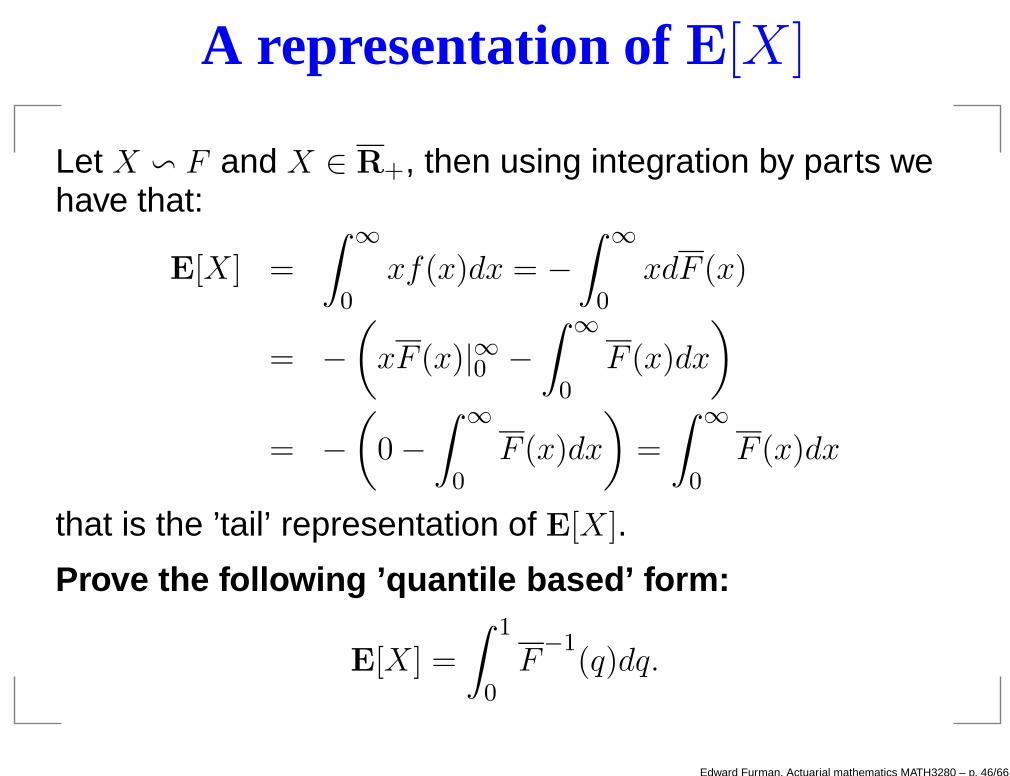
A representation of E[X ]

Let X v F and X ∈ R+, then using integration by parts wehave that:

E[X] =

∫ ∞

0xf(x)dx = −

∫ ∞

0xdF (x)

= −

(

xF (x)|∞0 −

∫ ∞

0F (x)dx

)

= −

(

0 −

∫ ∞

0F (x)dx

)

=

∫ ∞

0F (x)dx

that is the ’tail’ representation of E[X].

Prove the following ’quantile based’ form:

E[X] =

∫ 1

0F

−1(q)dq.


Some characteristics of life tables

Definition 6 The expected value of T (x) is denoted byex

and is referred to as the complete expectation of life.

Due to the above definition and from the tail representationof the mathematical expectation:

ex = E[T (x)] =

∫ ∞

0tpxdt.

It can be easily shown (just as in the case of E[X]) that:

E[X2] = 2

∫ ∞

0xF (x)dx,

thus leading to:

E[T (x)2] = 2

∫ ∞

0ttpxdt.


For the variance, we have that:

Var[T (x)] = E[T (x)2] − E2[T (x)]

= 2

∫ ∞

0ttpxdt −

(

ex

)2.

Definition 7 The median future lifetime of (x) is denoted bym(x), and it can be found by solving:

P (T (x) > m(x)) = m(x)px =S(x + m(x))

S(x)= 0.5

for m(x).

Definition 8 The mode for (x) can be obtained as:

arg maxt∈R+

tpxµ(x + t).


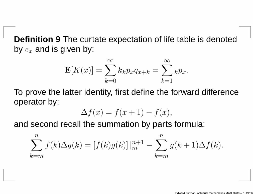
Definition 9 The curtate expectation of life table is denotedby ex and is given by:

E[K(x)] =

∞∑

k=0

kkpxqx+k =

∞∑

k=1

kpx.

To prove the latter identity, first define the forward differenceoperator by:

∆f(x) = f(x + 1) − f(x),

and second recall the summation by parts formula:n∑

k=m

f(k)∆g(k) = [f(k)g(k)] |n+1m −

n∑

k=m

g(k + 1)∆f(k).


Then:

ex =∞∑

k=0

kP (K(x) = k)

=

∞∑

k=0

k (P (K(x) ≤ k) − P (K(x) ≤ k − 1))

=∞∑

k=0

k (k+1qx − kqx)

=∞∑

k=0

k∆kqx =∞∑

k=0

k∆(1 − kpx)

= −∞∑

k=0

k∆kpx.


And hence, using the summation by parts:

ex = −

(

kkpx|∞0 −

∞∑

k=0

k+1px∆k

)

=

∞∑

k=0

k+1px =

∞∑

k=1

kpx,

bearing in mind that ex is finite.

Applying the same technique, we arrive at:

E[K(x)2] =∞∑

k=0

k2kpxqx+k,

thus yielding


= −∞∑

k=0

k2∆(kpx)

= −k2kpx|

∞0 +

∞∑

k=0

k+1px∆k2

=∞∑

k=0

(2k + 1)k+1px

=

∞∑

k=1

(2k − 1)kpx.

Finally, in this case:

Var[K(x)] =

∞∑

k=1

(2k − 1)kpx − e2x.


More characteristics

Definition 10 The function Tx is defined as:

Tx =

∫ ∞

0lx+tdt =

∫ ∞

x

lydy,

and it represents the expected total future lifetime of agroup of lx individuals all aged x.

To understand the interpretation, recall that:

ex =

∫ ∞

0tpxdt =

∫ ∞

0

lx+t

lxdt.

Thus, due to Definition 10:

Tx = lxex,

motivating the definition.


Definition 11 The function Lx is defined as:

Lx =

∫ 1

0lx+tdt =

∫ x+1

x

lydy,

and it denotes the total expected time lived between ages xand x + 1 by lx lives aged x.This time the interpretation can be seen from, e.g.,

Lx = Tx − Tx+1.

Definition 12 The central rate of mortality is defined as:

mx =

∫ 10 lx+tµ(x + t)dt∫ 10 lx+tdt

=dx

Lx,

which is the weighted average force of mortalityexperienced between ages x and x + 1 with weight lx+t atage x + t.


Recursion formulas

Example 10 Prove the following recursions for ex,ex:

u(x) = c(x) + d(x)u(x + 1) and u(x + 1) = −c(x)

d(x)+

1

d(x)u(x).

Solution Let us first check the left hand side for ex:

ex =

∞∑

k=1

kpx = px +

∞∑

k=2

kpx = px + px

∞∑

k=1

kpx+1 = px + pxex+1,

thus u(x) = ex, c(x) = d(x) = px, u(∞) = 0. In the case ofex:

ex =

∫ ∞

0tpxdt =

∫ 1

0tpxdt +

∫ ∞

1tpxdt

=

∫ 1

0tpxdt + px

∫ ∞

0tpx+1dt =

∫ 1

0tpxdt + px

ex+1.


Elementary numerical integration

Figure 9: Trapezoidal approximation for integrals.

According to the plot, the trapezoidal approximation is:∫ b

a

f(x)dx ≈ (b − a)f(b) +1

2(b − a) (f(a) − f(b))

=1

2(b − a) (f(a) + f(b)) .


Recursion formulas - cont.

Thus, we have that

u(x) =ex, c(x) =

∫ 1

0tpxdt, d(x) = px, u(∞) = 0.

Here, we can approximate c(x) with the trapezoidalapproximation:

c(x) =

∫ 1

0tpxdt ≈ px +

1

2(1 − px) =

1

2(1 + px) .

How do we obtain the second approximation?


One more example

Example 11 Show that under the UDD assumption, wehave that:

ex = ex + 0.5.

Solution Due to Definition 6, we have that:

ex =

1

lx

∫ ∞

0lx+tdt =

1

lx

∞∑

k=0

∫ 1

0lx+k+tdt

≈1

lx

∞∑

k=0

∫ 1

0((1 − t)lx+k + tlx+k+1) dt

=1

lx

∞∑

k=0

(

1

2lx+k +

1

2lx+k+1

)

=1

lx

(

1

2lx +

∞∑

k=1

lx+k

)

=1

2+ ex


Select life tables

Assumption 2 Let (x) possess a different probability thanthe general population of surviving to the next year for eachof the first k years after selection (the select period).Definition 13 We denote by:

tp[x]+r = 1 − tq[x]+r

the probability that (x + r) selected at age x will survive atleast next t years.All the relations we have seen hitherto hold, i.g.

t+sp[x]+r = tp[x]+r · sp[x]+r+t.

Assumption 3 Persons aged (x), selected before a numberof years that is bigger than r have the same survivalprobabilities, i.e., for all j > 0,

tp[x]+r = tp[x−j]+r+j .Edward Furman, Actuarial mathematics MATH3280 – p. 59/66

In simpler words, if k = 2, then:

q[x]+2 = q[x−1]+3 = q[x−2]+4 = · · · = qx+2.

In general, the select life table is constructed by workingback from lx+r successively to l[x]+r−1, l[x]+r−2, . . . , l[x] usingthe select probabilities p[x]+r−1, p[x]+r−2, . . . , p[x]. Moreprecisely, for all r ≥ 0,

l[x]+r =l[x]+r+1

p[x]+r

.

Example 12 Let k = 1 and an individual is aged x onselection. Then l[x] = lx+1/p[x]. Also, l[x]+1 = lx+1 for k = 1.We can further find e.g.

e[x] ≈

1

2+ e[x] =

1

2+

1

l[x]

∞∑

r=1

lx+r =1

2+

lxl[x]

ex,


which after another approximation reduces to:

e[x] ≈

1

2+

lxl[x]

(

ex −

1

2

)

.

Example 13 Let k = 2 and an individual is aged x onselection. Then l[x]+1 = lx+2/p[x]+1 and l[x] = l[x]+1/p[x]. Also,

e[x] ≈

1

2+ e[x] =

1

2+

1

l[x]

(

l[x]+1 +∞∑

r=2

lx+r

)

=1

2+

1

l[x]

(

l[x]+1 + lx+1ex+1

)

≈1

2+

1

l[x]

(

l[x]+1 + lx+1

(

ex+1 −

1

2

))

.


Figure 10: A 1967-70 mortality life table for assured lives.


The deterministic approach

A deterministic survivorship group as it is represented bythe life tables

initially consists of l0 lives aged 0,

is a subject to the annual rate of mortality (decrement) qx,

is closed, i.e., no entrances are allowed - onlydecrements.

Thus the progress of the group is determined by:

l1 = l0(1 − q0) = l0 − d0

l2 = l1(1 − q1) = l1 − d1 = l0 − (d0 + d1)...

lx = lx−1(1 − qx−1) = lx−1 − dx−1 = l0 −x−1∑

j=0

dj .


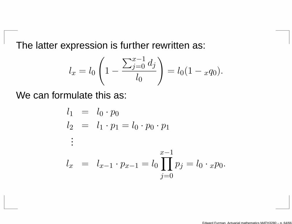
The latter expression is further rewritten as:

lx = l0

(

1 −

∑x−1j=0 dj

l0

)

= l0(1 − xq0).

We can formulate this as:

l1 = l0 · p0

l2 = l1 · p1 = l0 · p0 · p1

...

lx = lx−1 · px−1 = l0

x−1∏

j=0

pj = l0 · xp0.


To conclude:

Some relations between interest rate functions and thepresent topic:

Compound interest Survivorship group

A(t) lx

nit = A(t+n)−A(t)A(t) nqx = lx−lx+n

lx

δt = lim∆t→0A(t+∆t)−A(t)

A(t)∆tµ(x) = lim∆t→0

lx−lx+∆x

lx∆x

= dA(t)A(t)dt

= − dlxlxdx


References

ReferencesBowers, N. L., Hickman, J. C., Nesbitt, C. J., Jones, D. A.and Gerber, H. U. (1997). Actuarial mathematics, 2ndedition, Society of Actuaries, Itasca, Illinois.De Moivre, A. (1725). Annuities on Lives, 3-125.Gompertz, B. (1825). “On the nature of the functionexpressive of the law of human mortality, and on a newmode of determining the value of life contingencies”,Philosophical Transactions of Royal Society, (Series A) 115,513 - 583.Makeham, W.M. (1867). “On the law of mortality”, Journalof the Institute of Actuaries 8, 301-310.Weibull, W. (1951). “A statistical distribution function of wideapplicability”, Journal of Applied Mechanics 18, 293-297.


Documents

Edward Furman - YorkU Math and Statsefurman/actmath2008/lecture2.pdf · Feel comfortable with the deterministic approach to life tables. Edward Furman, Actuarial mathematics MATH3280