Download pdf - (8) Gait and stance (1)

172

Humans are bipedal creatures who rely on appendages known as legs as the primary means of lo-comotion. The human legs are the lower limb of the body. They extend from the hip to the ankle, encompassing the knee and everything in between. The legs are simple instruments, and yet the complex coordination among each component in it is able to generate the required force and mo-tion to move the body forward. This movement is called gaiting. Gaiting is defined as the manner in which locomotion is achieved by using the human limbs. Some common forms of human gaiting are walking, running, crawling, and hopping. Each of them requires varying starting orientations, stopping motions, changes in speed, alternations in direction, and modifications for changes in slope [1].

The motivation to understand the processes of human gaiting are beginning to take root in the medical world. The need for artificial legs by amputees to experience a normal daily life has pushed early medical pioneers to build various models for the legs. However, these models were too primitive to account for the complicated nature of gaiting. Today, rapid developments in biomedical research have provided the resources to finally make better advances in discovering the underlying mechanics of gaiting. Apart from restoring amputees, understanding human leg motions can pro-vide a standard or a reference to compare normal and abnormal gaiting that is a result from pain, paralysis, tissue damage, or other motor control dysfunction. This would perhaps provide better efficiency in detecting, and possibly curing, those problems.

The modeling of the human gait focuses on three components of the leg. The hips, knee, and ankle are the primary areas of research. Although all these three parts work together to provide mo-tion, there have been only isolated studies for each. Many articles and journals provide insight on only one of the three components. This could be because the coordination of all three is relatively complex and would require an excess of resources to combine them. One known application for all three would be the construction of robots to mimic human gaiting. Scientists in Japan had produced a mechanical automaton called the ASIMO (Advanced Step in Mobility). The ASIMO is a robot built specializing in emulating human gaiting. Much of the work on the robot focuses on balance and coordination. The motion of the legs can be easily emulated, but without coordination and feedback among the hips, knee, and ankle, the robot continues to fumble in its initial design [5].

Gait and Stance Control System

GAIt ANd StANCe CoNtroL SySteM 173

The leg structure is commonly characterized by a set of interconnecting pendulum systems. In Figure 16.1, it can be observed that the first pendulum system begins from the hip to the knee. The swinging angle from the hip will determine the displacement of the knee. A second pendulum system connects the knee to the ankle. Knee movements provide for the position on how the ankle lands. During gaiting, two different situations arise in sequence: the statically stable supported phase, in which the whole body is kept aloft by both legs simultaneously; and the statically unstable support phase, in which only one foot is in contact with the ground while the other is being trans-ferred from the back to the front. In a single walking cycle, the kinematic structure of locomotion changes from an open to a closed kinematic chain [4].

The coordination of the interconnecting pendulum assumptions can be further observed the simple gaiting (walking) process in Figure 16.2. The human walking is a process of locomotion in which the erect, moving body is supported by first one leg and then the other; as the moving body passes over the supporting leg, the other leg swings forward in preparation for its next support phase. One foot of the other is always on the ground, and during that period when the support of the body is transferred from the trailing to the leading leg there is a brief period when both feet are on the ground [2].

As walking speed increases, the periods of double support become smaller fractions of the walking cycle until, eventually, as a person starts to run, they disappear altogether and are replaced by brief periods when neither food is on the ground. The cyclic alternations of the support function of each leg and the existence of a transfer period when both feet are on the ground are essential features of the locomotion process known as walking.

FIGure 16.1: The leg system of the human body.

174 BASIC FeedBACK CoNtroLS IN BIoMedICINe

In attempting to understand the processes of gaiting and to combine the models for the hips, knee, and ankle together, Figure 16.3 displays the logic of a model. The pelvis, or the hips, is set as the starting point with the ankle as the ending point. The hips would receive an input signal from the cen-tral nervous system (CNS) or the peripheral nervous system, which is dependent on the type of action intended. Mainly for our model, input would come from the CNS; there will be no reflex reactions. The hip would influence the knee, and in turn the knee would determine the reaction of the ankle. The system of communication between the three components is in series with feedbacks coming out from each of their respective outputs. The final output would be a change in displacement or position [3].

Several assumptions were made for the modeling. The whole gating process is assumed to take place from the hips and down. The process for moving is totally isolated to just the coordina-tion between the hips, knee, and ankle. There will also be no additional loads applied to the legs other than the upper body. The legs will just be carrying the mass of the entire human body and will not be subjected to external forces. The walking surface for the leg model is assumed to be a flat surface with adequate friction coefficient for motion. Because the model focuses on the lower body,

FIGure 16.2: The phases of a normal gaiting process (breeze walking).

FIGure 16.3: The block diagram of the mechanical gaiting coordination system.


FIGure 16.4: Mechanical model for the hips.

influence from the vestibular feedback input and visual perception are ignored. The legs are made to act independently of their input. The arms will not be involved in balancing the body while in motion. Also, the legs are assumed to be in two-dimensional motions.

The model is first broken into the common three components; the hips, knee, and ankle. Each of these segments will be individually observed. Transfer functions were obtained for each component. Laboratory Virtual Instrumentation Engineering Workbench (LabVIEW) virtual in-struments (VIs) were also constructed to simulate the transfer function’s responses, and then Bode plots, root locus, and Nyquist plots were developed for each transfer function. Finally, all segments were combined together to form an overall system that represent the entire leg. Again, LabVIEW was used to simulate the entire leg’s response.

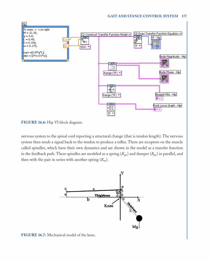
16.1 tHe HIPThere are not many models that describe the human hip; hence, the mechanical model use in the LabVIEW program is shown in Figure 16.4. This part of the leg is modeled as a thighbone with an actuator behind the bone. An analytic relation between the force provided by the actuator and the torque needed to move the articulation has been found. In particular, the segment k represents the arm of the hip joint torque for the model. The reaction force due to gravity is Mg, where M is the mass of the leg, and g is the gravitational acceleration due to gravity. The length of the thigh-bone is L, and from the diagram, k is found to be a proportion of L, in this case 0.7. The angle ω is between the actuator and the arm of the hip joint torque, and is treated as constant for this model. From observation, is it assumed to be 10° or 0.175 rad.

P (s) =

MgLksin( )

ss 2 + 1ω


whereL = length of thighbone = 48 cm = 0.48 mM = mass of leg (men, 19.5–25.2 kg; women, 11.7–16.6 kg)g = acceleration due to gravity (9.80 m/s2)k = arm of the hip joint torque, estimated from diagram to be 70% of L = 33.6 cmω = estimated to be 10° (= 0.175 rad), low angle so sin(ω): ω = 0.175

Figures 16.5 and 16.6 show the LabVIEW front panel view and block diagram, which contain the control VIs used in developing the LabVIEW hip program.

16.2 tHe KNeeTo model the human knee, the tendon can be treated as a small torsional spring damper with inertia ( J ), stiffness (K ), and damping (B) (Figure 16.7) Engineers try to estimate these parameters through experimental data from real human knees. When the tendon is excited, a signal is sent through the

FIGure 16.5: Hip VI front panel.


nervous system to the spinal cord reporting a structural change (that is tendon length). The nervous system then sends a signal back to the tendon to produce a reflex. There are receptors on the muscle called spindles, which have their own dynamics and are shown in the model as a transfer function in the feedback path. These spindles are modeled as a spring (Kpe) and damper (Bpe) in parallel, and then with the pair in series with another spring (Kse).

FIGure 16.6: Hip VI block diagram.

FIGure 16.7: Mechanical model of the knee.


Figure 16.8 is a commonly used block diagram to reason out the process of the knee,where

S(s) = 1

Kse(Bpe s + Kpe) For the feedback system,

G(s) =

G(s)1 +G(s)H(s)

Therefore,

G1 (s) =

1Js

1 +BJs

= 1Js + B

G2 (s) =

1Js 2 + Bs

1 + KJs 2 + Bs

= 1Js 2 + Bs +K

where B = 2.4382, J = 0.19033, K = 42.361, Kpe = 4.7627, Bpe = 0.96703, and Kse = 0.10774.Figures 16.9 and 16.10 show the LabVIEW front panel view and block diagram, which con-

tain the control VIs used in developing the LabVIEW knee program.

FIGure 16.8: Block diagram of knee.


FIGure 16.9: Front panel of knee.

FIGure 16.10: Block diagram of knee.


16.3 tHe ANKLeHuman standing posture in sagittal plane, as approximated to an inverted pendulum, is an unstable system and requires to be stabilized. Several sensory organs seem to be used for stabilizing the up-right posture in normal subject. The skeletal system of the standing posture is approximated as an inverted pendulum in sagittal plane as shown in Figure 16.11. Knee and hip joints were fixed by brace and ignored. Although the sway of the pendulum is small, the inertia of the skeletal system, viscosity, and elasticity of the muscle, and gravity effect can be described as a two-order delay dy-namics. A proportional, integral, and derivative (PID) controller is applied to M(s) and G(s). The muscle characteristic is approximated to one-order delay and dead time. The feedback parameters can be decided by a model matching method similar to the PID joint controller design. The block diagram of the ankle process is shown in Figure 16.12.

From the dynamics of human ankle stiffness, the transfer function G(s) is given as

G(s) =(s)

T (s)=

1

Js 2 + Bs + K −mgl

2

θ

whereθ(s) = ankle joint angleT(s) = moment of ankle joint torque; at 20 Nm external torque

FIGure 16.11: Mechanical model of ankle.


J = moment of ankle joint inertia (0.008 N m s2/rad)B = moment of ankle joint viscosity (10 N m s/rad)K = moment of ankle joint elasticity (240 N m/rad)m = mass of human (80 kg)l = height of human (1.7 m)

FIGure 16.12: Block diagram of the ankle process.

FIGure 16.13: Front panel of ankle.


Then, with 0 external torque, M(s) is calculated as

M(s) =

Kme−Ds

1 + sτ where

Km = gain of muscle (31 N m/rad)t = time constant of muscle (=0.1 s for f = 10 Hz)D = dead time of muscle (~350 µs)

G1 (s) = M(s)G(s) =

1


2

Kme−Ds

1 + s

G1 H (s) =

1


2

Km e−Ds

1 + s

1 +

1


2

Kme−Ds

1 + sKp +Kd s

=1


21 + s

Km e−Ds+ Kp + Kds

τ

τ

τ

FIGure 16.14: Block diagram of ankle.


G2(s) = G1 H (s)Ki

s=

K i


21 + s

Kme− Dss + Kp s + Kd s 2

τ

Gx(s) =

Ki


21 + s

Km e− Ds s + Kp s + Kd s 2

1 +Ki


21 + s

Km e− Dss + Kp s + Kd s 2

=Ki


21 + s

Km e− Dss + Kp s + Kd s 2 + Ki

τ

τ

τ

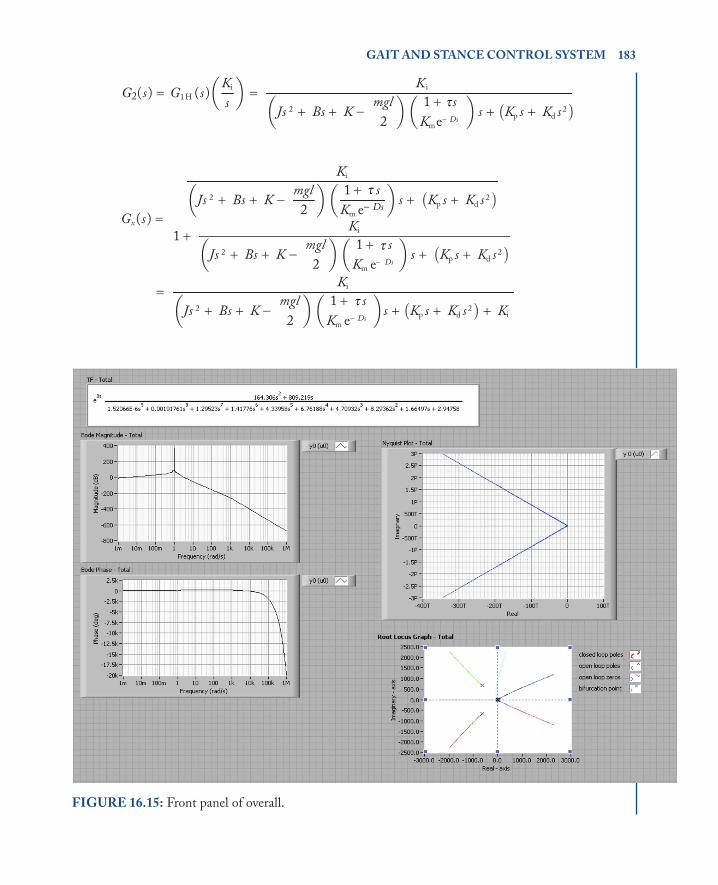
FIGure 16.15: Front panel of overall.


FIGure 16.16: Block diagram of overall.

Figures 16.13 and 16.14 show the LabVIEW front panel view and block diagram, which contain the control VIs used in developing the LabVIEW ankle program.

16.4 oVerALL SySteMFigures 16.15 and 16.16 are the modeling of the overall system in LabVIEW. All the transfer functions obtained are assumed to work in series. The response of the system is simulated and dis-played.


reFereNCeS[1] Rose, J., and Gamble, J. G., Human Walking, 3rd ed., Lippincott Williams & Wilkins,

Philadelphia (2006).[2] Giannini, S., Catani, F., Benedetti, M. G., and Leardini, A., Gait Analysis: Methodologies

and Clinical Applications, 1st ed., IOS P, Amsterdam, Netherlands (1994).[3] Vaughan, C. L., Davis, B. L., and O’Connor, J. C., Dynamics of Human Gait, Human Kinet-

ics, Campaign, IL (1992).[4] Muscato, G., and Spampinato, G., Kinematical model and control architecture for a human

inspired five DOF robotic leg, Mechatronics, 17, 45–63 (2007), <http://www.sciencedirect .com/science/article/B6V43-4KVXPKF-1/1/090b0a36e51f67445c5a4ceaad969241>, ac-cessed 2 Apr. 2008.

[5] Kim, J.-Y., Park, I. W., and Oh, J.-H., Experimental realization of dynamic walking of the biped, Adv. Robotics, 20, 707–736 (2006).

• • • •

http://www.sciencedirect.com/science/article/B6V43-4KVXPKF-1/1/090b0a36e51f67445c5a4ceaad969241

http://www.sciencedirect.com/science/article/B6V43-4KVXPKF-1/1/090b0a36e51f67445c5a4ceaad969241