SENSOR-LESS VECTOR CONTROL USING ADAPTIVE OBSERVER
SCHEME FOR CONTROLLING THE PERFORMANCE OF THE INDUCTION
MOTOR
MAZHAR HUSSAIN ABBASI
RESEARCH REPORT SUBMITTED IN PARTIAL
FULFILLMENT OF THE REQUIREMENT FOR THE
DEGREE OF MASTER OF ENGINEERING
FACULTY OF ENGINEERING
UNIVERSITY OF MALAYA
KUALA LUMPUR
2013
Univers
ity of
Mala
ya

ii
ORIGINAL LITERARY WORK DECLARATION
Name of the candidate: Mazhar Hussain Abbasi
Registration/Matric No: KGZ110007
Name of the Degree: Master of Engineering (Mechatronics)
Title of Project Paper/ Research Report/ Dissertation / Thesis (“this work”):
Sensorless vector control using adaptive observer scheme for controlling the
performance of induction motor
Field of Study: Electrical machines and drives
I do solemnly and sincerely declare that:
(1) I am the sole author /writer of this work;
(2) This work is original;
(3) Any use of any work in which copyright exists was done by way of fair dealings and
any expert or extract from, or reference or reproduction of any copyright work has been
disclosed expressly and sufficiently and the title of the Work and its authorship has been
acknowledged in this Work;
(4) I do not have any actual knowledge nor ought I reasonably to know that the making
of this work constitutes an infringement of any copyright work;
(5) I, hereby assign all and every rights in the copyrights to this work to the University
of Malaya (UM), who henceforth shall be owner of the copyright in this Work and that
any reproduction or use in any form or by any means whatsoever is prohibited without
the written consent of UM having been first had and obtained actual knowledge;
(6) I am fully aware that in the course of making this Work I have infringed any
copyright whether internationally or otherwise, I may be subject to legal action or any
other action as may be determined by UM.
Candidate’s Signature Date:
Subscribed and solemnly declared before,Witness Signature Date:Name:Designation:
Univers
ity of
Mala
ya

iii
ACKNOWLEDGEMENT
First of all, I would like to express my gratitude to the Almighty Allah, who has created
and gave me strength to finish the dissertation successfully. I remember the esteem,
affection and inspiration of my entire family to complete the degree successfully. I
would like to bestow my gratitude and profound respect to my supervisor Prof. Dr.
Velappa Gounder Ganapathy for his hearty support, encouragement and incessant
exploration throughout my study period.
I am specially acknowledging Mrs. Armarosa for her kind encouragement and
motivation.
I gratefully acknowledging the privileges and opportunities offered by the University of
Malaya. I also express my gratitude to the staff of this varsity that helped directly or
indirectly to produce this piece of work.
Univers
ity of
Mala
ya

iv
ABSTRACT
Sensorless vector control technique using adaptive observer scheme is being used to
control the performance of induction motor which is demonstrated by the help of
matlab/simulink software; a suitable tool for vector control of AC motor. Simulation is
done by using the observer which uses optimal feedback gain as an example of process
from algorithm design to verification of logic. Control design scheme in vector control,
accuracy of internal parameter such as resister of motor armature and inductance affects
control performance. Internal parameters are used, for example, feed-forward
compensator of current controller and parameters of observer model in sensor less
position.
The same technique also can be applied to other types of motor like PMSM. This
adaptive observer is used with the field oriented control of the induction motor. It is
based on using induction motor model with the estimation of the load torque besides the
estimation of the stator resistance and the robustness of this adaptive observer is with
respect to the variation in the resistance of stator. The performance of the suggested
adaptive observer scheme is present on via numerical simulation and the obtained
results from that adaptive observer show the effectiveness of suggested scheme.
Univers
ity of
Mala
ya

v
ABSTRAK
Teknik kawalan vektor tanpa sensor menggunakan skim pemerhati penyesuaian yang
digunakan untuk mengawal prestasi motor aruhan yang ditunjukkan oleh bantuan
perisian MATLAB / SIMULINK; alat yang sesuai untuk kawalan vektor AC motor.
Simulasi dilakukan dengan menggunakan pemerhati yang menggunakan perolehan
maklum balas yang optimum sebagai contoh proses daripada reka bentuk algoritma
untuk pengesahan logik. Skim reka bentuk kawalan dalam kawalan vektor, ketepatan
parameter dalaman seperti rintangan daripada angker motor dan kearuhan
mempengaruhi prestasi kawalan. Parameter dalaman digunakan, sebagai contoh,
pengawal arus pengimbang pemacu-hadapan dan parameter model pemerhati dalam
kedudukan tanpa sensor.
Teknik yang sama juga boleh digunakan untuk lain-lain jenis motor seperti PMSM.
Pemerhati penyesuaian ini digunakan dengan kawalan berorientasikan medan motor
aruhan tersebut. Ini berdasarkan menggunakan model motor aruhan dengan anggaran
tork beban selain anggaran rintangan pemegun dan kekukuhan pemerhati penyesuaian
ini adalah berkenaan dengan perubahan dalam rintangan pemegun. Prestasi cadangan
skim pemerhati penyesuaian ini dibentangkan melalui simulasi berangka dan keputusan
yang diperolehi daripada pemerhati penyesuaian itu menunjukkan keberkesanan skim
yang disyorkan.
Univers
ity of
Mala
ya

vi
TABLE OF CONTENTS
ORIGINAL LITERARY WORK DECLARATION .........................................................ii
ACKNOWLEDGEMENT ...............................................................................................iii
ABSTRACT.....................................................................................................................iv
ABSTRAK ........................................................................................................................v
LIST OF TABLES............................................................................................................ix
LIST OF FIGURES...........................................................................................................x
CHAPTER ONE: INTRODUCTION ...............................................................................1
1.1 Objectives:...............................................................................................................4
1.2 Outline of the project report: ...................................................................................4
CHAPTER TWO-LITERATURE REVIEW ....................................................................6
2.1 Introduction .............................................................................................................6
2.2 Speed-Sensorless control.........................................................................................7
2.3 Speed estimation schemes of sensorless induction motor drives ............................8
2.3.1 Rotor Slot Harmonics (RSH) Method ..............................................................9
2.3.2 Frequency Signal Injection (FSI) Method ......................................................10
2.4 Machine Model (MM) Methods............................................................................ 11
2.4.1 Direct calculation method (DCM) ..................................................................12
2.4.2 Model reference adaptive system ...................................................................14
2.4.2.1. Rotor Flux-Based MRAS............................................................................15
2.4.2.2. Back emf-Based MRAS..............................................................................16
Univers
ity of
Mala
ya
vii
2.4.2.3. Stator Current-Based MRAS ......................................................................17
2.5 Kalman Filter approach .........................................................................................20
2.6. Artificial intelligence techniques ..........................................................................22
2.6.1 Neural Network based model .........................................................................23
2.6.2 Fuzzy logic based model.................................................................................24
2.7 Sliding mode observer (SMO): .............................................................................26
2.8 Speed estimation at low speed...............................................................................28
2.8.1 Data Acquisition Errors ..................................................................................29
2.8.2 Voltage Distortion due the Pulse Width Modulation (PWM) Inverter ...........29
2.8.3 Stator Resistance Drop....................................................................................30
2.9 Parameter Adaption ...............................................................................................30
2.10 Adaptive flux observer (AFO).............................................................................33
2.11 Final summarise comments .................................................................................35
CHAPTER THREE: METHODOLOGY .......................................................................38
3.1 Basic Principles of Vector Control ........................................................................38
3.2 System Modelling..................................................................................................40
3.2.1. Description of Symbols .................................................................................42
3.2.2 Subscript symbol description..........................................................................42
3.2.3 Description of signal label ..............................................................................44
3.3 Principles and Analysis Model Sensorless velocity by Adaptive Secondary Flux
Observer ......................................................................................................................49
3.4 Modeling of Adaptive observer .............................................................................53
Univers
ity of
Mala
ya

viii
CHAPTER FOUR: RESULTS AND DISCUSSION......................................................56
4.1 Discussion of results..............................................................................................68
CHAPTER FIVE: CONCLUSION AND RECOMENDATION....................................69
5.1 Conclusion.............................................................................................................69
5.2 Recommendation...................................................................................................70
REFERENCES................................................................................................................71
Univers
ity of
Mala
ya

ix
LIST OF TABLES
Table 2. 1 Advantages and distadvantage of MRAS method..........................................20
Table 2. 2 Comparison of different methods regarding estimation speed.......................36
Table 2. 3 Grading on merit based of speed estimation ..................................................36
Table 4. 1 IM parameters and value for M-file ...............................................................56
Univers
ity of
Mala
ya

x
LIST OF FIGURES
Figure 1. 1 Related optional tool together with controller development process .............3
Figure 3.2.1 Flow chart of basic vector principle…………………………...………….39
Figure 2. 1 Block diagram of speed estimation based on rotor slot harmonics(Holtz
2002) ...............................................................................................................................10
Figure 2. 2 Speed estimation method based on signal injection(Hinkkanen, Leppanen et
al. 2005)........................................................................................................................... 11
Figure 2. 3 Rotor speed estimation Block diagram structure based on direct calculation
method (Wolbank, Woehrnschimmel et al. 2000) ...........................................................13
Figure 2. 4 Using the MRAS the block diagram of rotor speed estimation
structure(Rashed and Stronach 2004) .............................................................................14
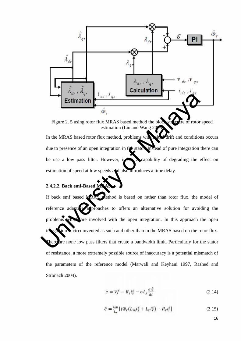
Figure 2. 5 using rotor flux MRAS based method the block structure of rotor speed
estimation(Liu and Wang 2008) ......................................................................................16
Figure 2. 6 Using back EMF based MRAS block diagram of rotor speed
estimation(Rashed and Stronach 2004)...........................................................................17
Figure 2. 7 Speed estimation configuration scheme by using the stator current based
MRAS method(Schauder 1992)......................................................................................19
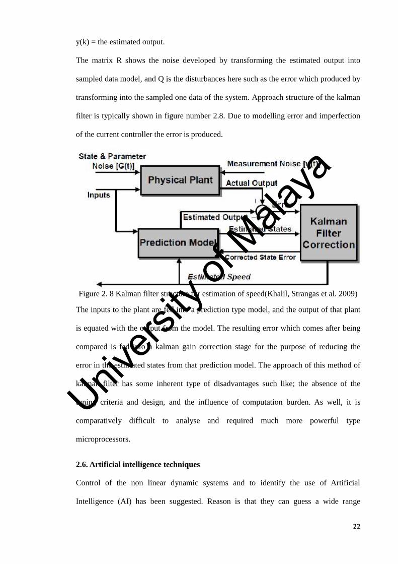
Figure 2. 8 Kalman filter structure for estimation of speed(Khalil, Strangas et al. 2009)
.........................................................................................................................................22
Figure 2. 9 Using Artificial NN model structure of the speed estimation(Wang, Lin et al.
2010) ...............................................................................................................................23
Figure 2. 10 type-2 Fuzzy logic Control(Venkataramana Naik and Singh 2012) ...........25
Figure 2. 11 PID controller with Fuzzy logic block diagram of induction motor(Lopez,
Romeral et al. 2006)........................................................................................................26
Figure 2. 12 Sliding Mode Observer (SMO) Block diagram (Lascu and Andreescu
2006) ...............................................................................................................................28
Univers
ity of
Mala
ya
xi
Figure 2. 13 speed estimation block diagram of Adaptive Observer(Tarek
BENMILOUD 2011).......................................................................................................34
Figure 2. 14 Different methods of speed estimation comparison chart ..........................37
Figure 3. 1 Three-phase fixed coordinate system ...........................................................38
Figure 3. 2 Two-phase fixed coordinate system and rotating coordinate system ...........39
Figure 3.2.1 flow chart of basic vector principle……………………………………….39
Figure 3. 3 Configuration Block diagram of position sensorless vector control ............41
Figure 3. 4 Modelling of controller part..........................................................................43
Figure 3. 5 Internal model of coordinate transformer subsystem “Rotating_to_Fixed” .46
Figure 3. 6 Internal model of coordinate transformer subsystem “Fixed_to_Rotating” .46
Figure 3. 7 Internal model of current controller subsystem ............................................47
Figure 3. 8 Modeling Example using SimPowerSystem ................................................48
Figure 3. 9 Adaptive Flux Observer Configuration Diagram .........................................50
Figure 3. 10 Current error block feedback system..........................................................52
Figure 3. 11 Model of Adaptive Observer.......................................................................54
Figure 3. 12 Block diagram inside the Matrix A.............................................................54
Figure 3.13 Bode diagram of linear time-invariant block………………………...……55
Figure 4. 1 Voltage between inverter UVs[V].................................................................58
Figure 4. 2 Three-phase stator current of motor [A] .......................................................59
Figure 4. 3 Motor rotating velocity [rpm].......................................................................60
Figure 4. 4 Motor rotating velocity [rpm].......................................................................61
Figure 4. 5 Motor rotating velocity [rpm].......................................................................62
Figure 4. 6 Motor rotating velocity [rpm].......................................................................63
Figure 4. 7 Electromagnetic Torque to 1 Nm..................................................................64
Figure 4. 8 Electromagnetic Torque to 50 Nm................................................................65
Figure 4. 9 Electromagnetic Torque to 1 Nm..................................................................66
Univers
ity of
Mala
ya

xii
Figure 4. 10 Electromagnetic Torque to 50 Nm..............................................................67
Univers
ity of
Mala
ya
xiii
LIST OF SYMBOLS
Resistor R
Self-inductance [H] L
Mutual inductance [H] M
Rotor flux rotation angle [rad] θ
Rotor flux angle velocity [rad/sec] ω
Electric angular velocity [rad/sec] ω
Current value [A] i
Voltage value [V] v
Electric torque [N] TFlux linkage λ
Number of pole pairs P
Laplace operator s
Variable in the stator s
Variable in the rotor r
Variables in three-phase fixed coordinate system U, V, W
Variables in orthogonal two-axis fixed coordinate system α,ß
Variables in orthogonal two-axis rotating coordinate system d, q
Target value *
Estimation value ^
Voltage target value on d and q axes vds, vqs
Voltage target values ona,ßaxes va, vb
Voltage target values on UVW axis vu, vv, vw
Current target values on d and q axes ids, iqs
Current value on UVW axis iu, iv, iw
Univers
ity of
Mala
ya

xiv
Current values on a and ß-axes ia, ib
Subscript indicating target value *
Rotor flux rotation angle (power supply angle) theta (ϴ)
Rotor flux rotating angler velocity (power supply angler velocity) w
Electric angler velocity estimation value wr
Rotor flux of α and ß-axes Ramd_ar, Ramd_br
Flux linkage λ
Number of pole pairs P
Laplace operator s
Univers
ity of
Mala
ya
1
CHAPTER ONE: INTRODUCTION
The sensorless vector control using feedback gain as an instance of process from the
algorithm design to logic verification using adaptive observer scheme for controlling the
performance of induction motor (Dr.JBV Subrahmanyam 2011, Tarek BENMILOUD
2011) by using MATLAB/Simulink is presented in the thesis. Nowadays, the direct
field oriented control (FOC) technique is outspread used in high performance induction
motor (IM) drives (J.P. Caron 1995),(Volat 2000). It permits the electromagnetic torque
control to be separated from the rotor flux one by the aid of coordinate transmission,
and thus to handle induction motor (IM) as dc motor. Such control method needs the
knowledge of the rotor flux, which is indirectly measurable. Rotor flux observers’ are
commonly used in order to avoid expensive sensors (Alamir 2002).
Knowing that the efficiency of the control strategy is established on right rotor flux
detection, the drive functioning is strictly connected to these of the rotor flux
observer(M. Alexandru 2002). Accordingly, the performances of the observer, in terms
of accuracy, stability and robustness censoriously influence those of the drive. In this
work, proposal for improving the performances and robustness of the adaptive flux
observer of induction motor, using the estimation of the load torque as an added input
for the adaptive observer is going to be considered. The estimation of the load torque
will provide profound estimation of the rotor flux, because the adaptive observer will
have more similarity to the real model of the induction motor. With the help of
simulation results, the effectiveness of the proposed scheme is being discussed. The
reasons depicted as below demonstrate that MATLAB/Simulink is a tool suitable for
vector control of Induction Motor in this thesis.
Univers
ity of
Mala
ya

2
Configuration of the vector control diagram can be expressed by Simulink block
diagram clarifying the signal stream through grouping and organizing function
unit as subsystem.
Easy to express matrix formula often used in system expression of motor.
Able to model and simulate multi domain systems such as mechanical and
electrical as like a simulator for mathematical expression model.
The embedded legacy of C code as controller and plant model can be verified
through the simulation in simulink block diagram.
Able to co-simulate with magnetic field analysis software, mechanical analysis
software and electric circuit simulator.
Optional toolboxes and extended block sets provide solutions for a wide variety
of development phases from algorithm design, verification, and prototype testing
to implementation.
Some of the “solutions provided for development phase” are listed below and what is
covered in this thesis is clarified as well.
Univers
ity of
Mala
ya
3
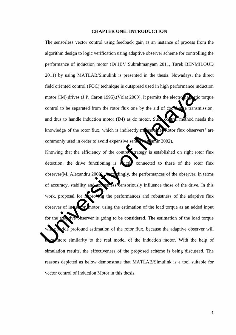
Figure1. 1 Related optional tool together with controller development process
Accuracy of internal parameter in vector control such as inductance and the resister of
motor armature affect control performance. Internal parameters are used, for instance,
parameters of observer model in position sensor less and feed-forward compensator of
current controller. In the process of 1 of figure 1.1, some methods are possible such as;
the same input voltage is applied to actual motor and motor modelled in Simulink, and
from the cost function that minimizes output current deviation, each parameter is
estimated in least square method. Data Acquisition Toolbox provides interface with
A/D, D/A boards, and allows acquisition of real signal by MATLAB program
execution. The Optimization Toolbox, function library providing various optimization
methods, is available for optimization calculation for parameter estimation(Ugale, Dond
et al. 2012).
Univers
ity of
Mala
ya

4
In the process of 2, Control System Toolbox is available for designing observer based
on modern control theory, and verifying its characteristic features(Korlinchak and
Comanescu 2012).
In the process of 3, simulation of the whole system is executed based on the parameters
and observers obtained from the processes 1 and 2.
The SimPowerSystems, electric systems library, provides inverter and motor blocks.
Because the prepared Motor block is an ideal model not including non-linearity such as
magnetic saturation, a method such as co-simulating with magnetic analysis tool is
considered in a more realistic simulation.
In the process of 4, xPC can be used for real-time simulation of actual motor, and tune
Simulink model while monitoring in signal time. The real time work shop (“RTW”) can
generate c-code from controller modelled by Simulink and implement on MPU or DSP.
On the other hand, as plant of simulation is ideal model, control parameter tuning might
be required for actual machine.
In the process of 5, with the good readability for production-quality code suitable for
implementation, performance and customization can be generated by combining add-on
tool of RTW, RTW Embedded Coder.
1.1 Objectives:
The Objectives of this work are as follows:
Design and analysis of adaptive observer for controlling the performance of
induction motor.
Get the controllable results of different parameters of induction motor by the
adaptive observer and recommendation for more reliable system.
1.2 Outline of the project report:
The remainder of this report is organised in the following manner:
Univers
ity of
Mala
ya

5
Chapter 2 provides the literature review of the different techniques of sensorless
control of induction motor. A detail study of all sensorless methods with their
advantages, disadvantages has been discussed along with the controlling schemes and
according to that review based comparison also discussed.
Chapter 3 deals with the methodology that has been implemented to control the
performance of induction motor by adaptive observer scheme. This chapter includes
comprehensive analysis on the different sections of the simulation that what controlling
technique is used in each of the section with mathematical operation.
Chapter 4 presents the results performed by simulation software-matlab at different
values in terms of changing the parameters of induction motor, on external load and at
different speeds for achieving the object of the project.
Chapter 5 summarizes all the study and analysis performed for the project and
enhances the future work with recommendation which can be done to get the more
accurate and reliable system.
Univers
ity of
Mala
ya
6
CHAPTER TWO-LITERATURE REVIEW
2.1 Introduction
For modern industrial applications the high performance based electric motor drives are
believed a crucial demand. Previously, the dc motors have been universally used for this
purpose. However, frequent maintenance, heavy weight and large size requirements
make the dc motors a highly expensive solution. Furthermore, mechanical assembly of
commutator-brush cause unwanted sparking, which is really not allowed in certain
practical applications. Such fundamental defect of dc motors motivated the researchers
for persistent efforts to find out the more beneficial solution to the problems, and many
successful efforts have been made to adopt induction motor instead of dc ones.
Induction motor has huge advantages like reliability, simplicity, virtually maintenance
free, and less expensive. Nevertheless, the time varying nature and nonlinearity of
induction motor drive requires a large amount of real-time computation and fast
switching power devices (M.S. ZAKY 2008).
Due to the recent developments in the field of power electronics using field oriented
control (FOC) technique, the accurate speed and torque control of induction motor is
now possible. FOC has two integral types of method known as Direct and Indirect
methods. The direct FOC method rely on generating unit vector signals, which are
required for flux orientation, and it comes from the fluxes measured by using the hall
effect flux sensor or also search the coils, or estimated. On the other hand, indirect field
oriented applies the speed of rotor and from the dynamic equation of the rotor usually
drive the slip angular frequency to generate the signals to achieve the orientation flux.
Despite the fact that the indirect motor is highly sensitive to the variations of motor
parameters, such us rotor time constant, still it is practically preferred than the direct
one. This is due to the direct method requires a modification or a particular design for
Univers
ity of
Mala
ya
7
the machine. Additionally, the breakability of the flux sensors frequently reduces the
inherent robustness of induction motor drive (Consoli, Scarcella et al. 2004).
2.2 Speed-Sensorless control
Realization of the high precision speed control and high performance of IM drives
information regarding accuracy of speed is always necessary. Traditionally, a direct
kind of speed sensors such as an encoder was usually mounted to the motor shaft and
the purpose was to measure the speed. Such methods uses the required additional
electronics, extra space, extra wiring, careful mounting and frequent maintenance which
takes away the reliability and inherent robustness of drives becomes expensive also due
to addition of extra cost in it.
Due to these reasons, the advancement of alternative option in indirect methods turn to
be an important research (Holtz 2002). Therefore, the research community have a great
motivation and interest to develop a speed sensorless IM drive. A lot of advantages are
expected from speed sensorless IM drives like reduced size, reduced hardware
complexity, better noise immunity; elimination of direct type of sensor writing, less
maintenance requirements and the most important one is the low cost, which is always a
top priority of industrial reasearchers. They are also preferred not for high speed
applications but also in hostile environments (Ilas, Bettini et al. 1994, Zaky 2012).
For the next generation of commercial motor drives, not only for induction machines,
but also include other machines, say for instance; permanent magnet synchronise
motors(PMSM) and switched reluctance motors(SRM), the positive features of
sensorless speed systems will be preferable (Sheng-Ming and Shuenn-Jenn 2000,
Rahman, Zhong et al. 2003).
Univers
ity of
Mala
ya
8
2.3 Speed estimation schemes of sensorless induction motor drives
Elimination of direct speed sensors of IM drives are successfully reported recently.
These attempts employ the parameters of IM and motor terminal variables in some way
to estimate the motor speed. A common notion arises like; to which extent the method
will succeed without deteriorating the dynamic performance of the drive. Recently,
several methods have been proposed for the estimation of speed for the high
performance of induction motor drives. Among those methods some are based on a
phenomenon of non ideal type such as rotor-slot-harmonics (Holtz 2002, Staines,
Caruana et al. 2006). Spectrum analysis is required for such methods, and that really is a
time consuming type procedures. They permit a very compact narrow band of
controlling the speed. An alternative class algorithm based on some type of probing
signals injected into terminals of stator (current and / or voltage) just to detect the rotor
flux and the speed of the motor accordingly (Hinkkanen, Leppanen et al. 2005, Holtz
2006). Such probing signals which introduce formerly a high frequency (Hz) torque
pulses and therefore speed ripple is the result in return. That is also the reason of
distortion of some useful data due to the interference with high Hz probing signals.
Despite of the reality regarding merit of such methods of estimation speed near zero
they undergo from very large calculation time also called computation time, also limited
bandwidth control and complexity. Alternatively, by using the terminal quantities like
current and voltage the speed information can be obtained (Schauder 1992, Marwali and
Keyhani 1997, Liu and Wang 2008). For this purpose it includes so many different
methods such as; Extended Kalman Filters(Smidl and Peroutka 2012), Model Reference
Adaptive Systems (MRAS)(Khan and Iqbal 2012), simple open loop speed calculators
(Tajjudin, Rahiman et al. 2012), Artificial Intelligence Techniques (Siddique, Yadava et
al. 2003) and adaptive flux observer (Lesan, Doumbia et al. 2012, Savoia, Verrelli et al.
2012). Methods based on model are characterised due to their good performance at high
Univers
ity of
Mala
ya
9
speed, also their simplicity. Nevertheless, they display the lower accuracy at low speed
mostly and it has reason of due to parameters variation. Speed estimation schemes of
speed-sensorless induction motor drives can be classified as follows:
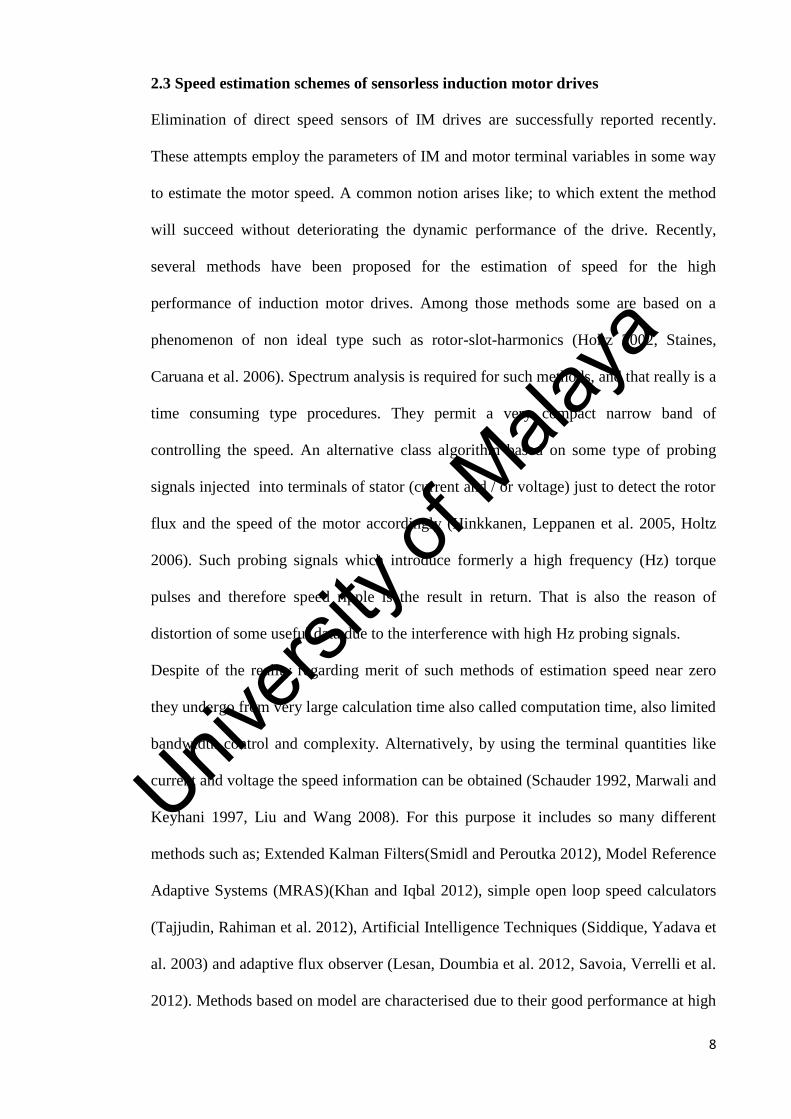
2.3.1 Rotor Slot Harmonics (RSH) Method
The process of speed calculation is based on detecting the space harmonics which are
induced by rotor slots (Holtz 2002, Staines, Caruana et al. 2006).Space harmonic
components are generated by the rotor slots in the air gap magneto motive force (mmf),
and that regulated the flux linkage of stator at a frequency which is proportional to the
speed of rotor and also to the number of rotor slots (Nr). Since Nr is generally not a
multiple of three, the rotor slots harmonics bring on voltage of harmonic in the phases
of stator and that comes along as triple harmonics with respect to the fundamental stator
voltage V .
V = V sin(N w ± w ) τ, (2.1)
Where Nr= 3n±1,
n = 1, 2, 3…
As all triple harmonics from the larger fundamental voltage can be easily separated
which are from sequence zero, and that sequence voltage denoted as vo is the sum of all
the three phase voltages which is connected in a wye-connected winding of stator.
Though adding the voltages of phase, all non-triple components also including the
basics, become sett off while the triple harmonics add up in it.
V = (V + V + V ) (2.2)
In order to isolate the signal which represents the angular velocity of the rotor
mechanical one, a band pass filter is employed which have adaptively tuned central
Univers
ity of
Mala
ya
10
frequency to the rotor slot harmonic frequency N w +w = Πτ
in equation (2.1). The
block diagram of speed estimation based on rotor slot harmonics is shown in Figure 2.1.
The harmonic rotor signal V is extracted by the adaptive band pass filter, and that
filtered signal is digitised by observing its zero crossing instants tz. On each zero
crossing through one count for memorizing the digitised position of rotor angle theta ϑ,
there is a software counter for increments and in the same way to that of encoder
increments by digital differentiation a slot frequency signal is then obtained. With
reference to Eqn. (2.1) the accurate speed of rotor is subsequently computed (Holtz
2002).
Figure 2. 1 Block diagram of speed estimation based on rotor slot harmonics(Holtz2002)
Problem with this technique as mentioned earlier that this approach required very high
precision measurements in which there is need to increase the hardware/software
complexity, which is not acceptable to industrials. Also, they suffer from large computation
time, complexity and limited bandwidth control.
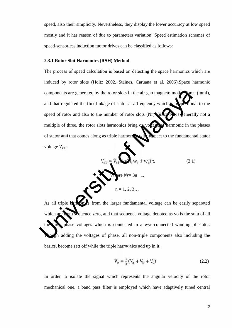
2.3.2 Frequency Signal Injection (FSI) Method
This method scheme for speed estimation is based on signal injection. Superimposition
of a high frequency voltage signal on the fundamental voltage is distinctively used to
excite the anisotropic phenomena of the motor, and the position of the rotor or the
direction of the flux is keyed out from the current response. This yielded for the
Univers
ity of
Mala
ya
11
comportment of the significant torque and therefore speed ripple. Also due to
interference with other signals of the same kind which carry the useful information may
be distorted. In addition, the common drawback of this method is that their dynamic
response is normally simply moderate (Hinkkanen, Leppanen et al. 2005, Holtz 2006).
Basic structure of speed estimation using the FSI method is shown in the fig.2.2, for the
performance of the current control in the field of coordinates an estimated filed angle δ
is used. Through the voltage signal = a revolving carrier frequency is
injected. The attenuation in the carrier frequency components in the measured machine
currents are by the low pass filter (LPF) in the feedback path of the controller of current.
Extraction of the carrier which generated current vector is by the bass pass filter
(BPF), and the speed of the rotor can be calculated by using the phase-locked loop
(PLL)(Holtz 2002).
Figure 2. 2 Speed estimation method based on signal injection(Hinkkanen, Leppanen etal. 2005)
2.4 Machine Model (MM) Methods
The outstanding deal of research interest is given to this category method of speed
estimation, which is based on machine model due to its simplicity. This section can be
sorted according to the algorithm being used for the estimation of speed. Detail of this
Univers
ity of
Mala
ya
12
machine model type of estimating the speed of motor can be sum up by the following
few methods.
2.4.1 Direct calculation method (DCM)
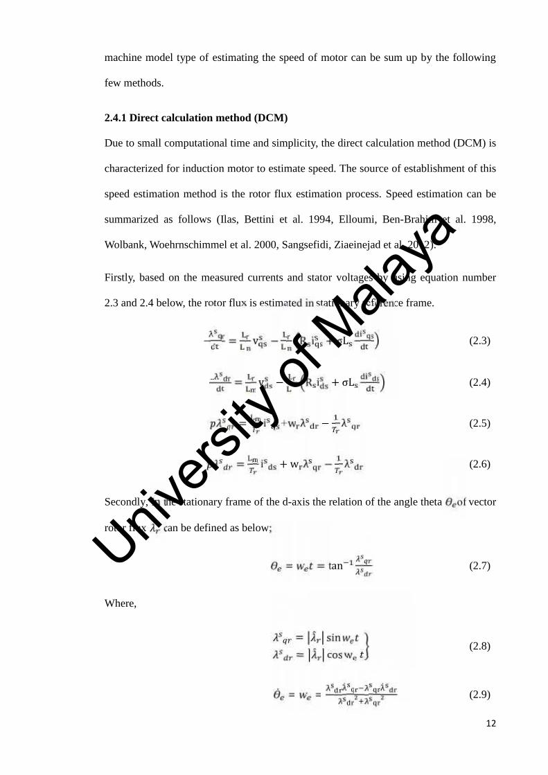
Due to small computational time and simplicity, the direct calculation method (DCM) is
characterized for induction motor to estimate speed. The source of establishment of this
speed estimation method is the rotor flux estimation process. Speed estimation can be
summarized as follows (Ilas, Bettini et al. 1994, Elloumi, Ben-Brahim et al. 1998,
Wolbank, Woehrnschimmel et al. 2000, Sangsefidi, Ziaeinejad et al. 2012).
Firstly, based on the measured currents and stator voltages by using equation number
2.3 and 2.4 below, the rotor flux is estimated in stationary reference frame.
= v − R i + σL (2.3)
= v − R i + σL (2.4)
= i +w λ − λ (2.5)
= i + w λ − λ (2.6)
Secondly, in the stationary frame of the d-axis the relation of the angle theta of vector
rotor flux can be defined as below;
= = tan (2.7)
Where,
= sin= cos w (2.8)
= = (2.9)
Univers
ity of
Mala
ya
13
Equation number 2.5 and 2.6 substitute in eqn. 2.9, the estimated rotor speed become;
= λ λ − λ λ − i − i (2.10)
Where,
= λ + λHence, given an overall knowledge of motor parameters, the Speed ω instantaneous
can be estimated from the equation 2.10. The process of all these is illustrated in the
below figure, number 2.3, estimation of rotor flux is necessity for calculation of rotor
speed as shown from the block diagram.
Figure 2. 3 Rotor speed estimation Block diagram structure based on direct calculationmethod (Wolbank, Woehrnschimmel et al. 2000)
When the frequency approaches to zero, there are three problems occurs related to the
rotor flux estimation. First, is that there is need of ideal integral which is necessary to
reach near to high result. Second, we need its sensitivity to variation of parameters
specially the resistance which has large influence at very low speed, and the 3rd one
is the influence of the dead-time when has the use of the actual stator voltage to the
pulse width modulation (PWM).
Univers
ity of
Mala
ya
14
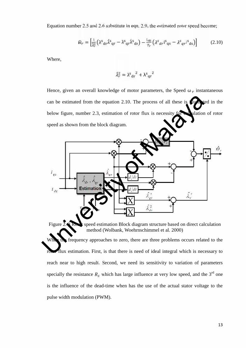
2.4.2 Model reference adaptive system
For sensorless induction motor drives, the model reference adaptive system (MRAS)
method is the one of the famous speed observers. It is one of many promising methods
technique employed in the adaptive control. Between various types of adaptive
configuration system, the MRAS is vital for a wide range of application. Since, it
contributes as to relatively easy in implementation of the systems with high speed of
adaption; this is one of the most notable advantages of the adaptive system. Due to the
fact, a measurement of the difference between the outputs of the reference model, and
the adjustable model is found right away by the comparison of the outputs or states of
the reference model along with those of the adjustable system. The demanded dynamics
of actual control loop are represented by the block “reference model”, and the block of
adjustable model represents the same structure as the reference one merely with
parameter of adjustable one. Instead of any unknown ones as shown in the figure
number 3.4, the consistence of the MRAS model basically is one on the reference
model, adjustable model and an adaptive mechanism.
Figure 2. 4 Using the MRAS the block diagram of rotor speed estimationstructure(Rashed and Stronach 2004)
The state variable is calculated by the independent reference model of the rotor speed
from the current and voltage terminal, and the dependent model on the rotor speed
Univers
ity of
Mala
ya
15
which is adjustable model estimate the state variable . For speed generation of the
estimated speed , use the error which is shown in the diagram between calculated and
estimated state variables.
From review of this technique, it is noted that the estimation of speed methods using MRAS
can be assorted in to several types following to that state variable. Among them the most
ordinarily used are the back emf-based MRAS, rotor flux-based MRAS, and the stator
current-based MRAS.
2.4.2.1. Rotor Flux-Based MRAS
As an output value the rotor flux is used in rotor Flux-Based MRAS method for the
model to estimate the speed of the rotor. Whilst the rotors flux of the method of
adjustable in equation number 2.12 is in conformity with that of reference model
equation number 2.11. The speed of the adjustable model represents as the real speed of
the rotor (Schauder 1992, Marwali and Keyhani 1997, Liu and Wang 2008).
= − − (2.11)
= − + (2.12)
Using the rotor flux based MRAS, the speed estimation algorithm is shown in the figure
2.5, and estimated speed of the rotor is expressed as;
= λ λ − λ λ + K ∫ λ λ − λ λ dt (2.13)Univers
ity of
Mala
ya
16
Figure 2. 5 using rotor flux MRAS based method the block structure of rotor speedestimation (Liu and Wang 2008)
In the MRAS based rotor flux method, problems with initial drift and conditions occurs
due to presence of an open integration in the stator. Instead of pure integration there can
be use a low pass filter. However, it has a capability of degrading the effect on
estimation of speed at low speeds and also introduces a time delay.
2.4.2.2. Back emf-Based MRAS
If back emf based MRAS method is based on rather than rotor flux, the model of
reference adaptive approaches to offers an alternative solution for avoiding the
problems which are involved with the open integration. In this approach the open
integration is circumvented as such and other than in the MRAS based on the rotor flux.
There are none low pass filters that create a bandwidth limit. Particularly for the stator
of resistance, a more extremely possible source of inaccuracy is a potential mismatch of
the parameters of the reference model (Marwali and Keyhani 1997, Rashed and
Stronach 2004).
= − − (2.14)
= [ ( + ) − ] (2.15)
Univers
ity of
Mala
ya
17
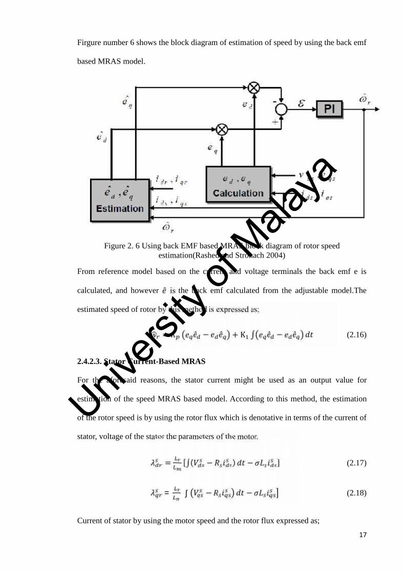
Firgure number 6 shows the block diagram of estimation of speed by using the back emf
based MRAS model.
Figure 2. 6 Using back EMF based MRAS block diagram of rotor speedestimation(Rashed and Stronach 2004)
From reference model based on the current and voltage terminals the back emf e is
calculated, and however is the back emf calculated from the adjustable model.The
estimated speed of rotor by this method is expressed as;
= − + K ∫ − (2.16)
2.4.2.3. Stator Current-Based MRAS
For the aforesaid reasons, the stator current might be used as an output value for
estimation of the speed MRAS based model. According to this method, the estimation
of the rotor speed is by using the rotor flux which is denotative in terms of the current of
stator, voltage of the stator the parameters of the motor.
= [∫( − ) − ] (2.17)
= ∫ − − (2.18)
Current of stator by using the motor speed and the rotor flux expressed as;
Univers
ity of
Mala
ya

18
= + + (2.19)
= + + (2.20)
Stator current is estimated as below by using the eqauation number 2.19 and 2.20 and
the estimated speed .
= + + (2.21)
= + + (2.22)
From the relationship of above calculated and estimated stator currents, the difference
which is in the stator current is received as;
− = ( − ) (2.23)
− = ( − ) (2.24)
Multiply and add equation (2.23) and (2.24) together with the flux of the rotor , we
have the following expression ;
(i − ı )λ + ı − i λ = (w − w ) λ + λ (2.25)
The error of the rotor speed we can write from the above equation number (2.25) as;
w − w = n (i − ı )λ + ı − i λ (2.26)
Where as;
n = LT 1( ) +Block diagram of stator current based method of MRAS is shown in the figure number
2.7. Whereas from equation (2.26) ,we determined the speed estimation error from the
Univers
ity of
Mala
ya
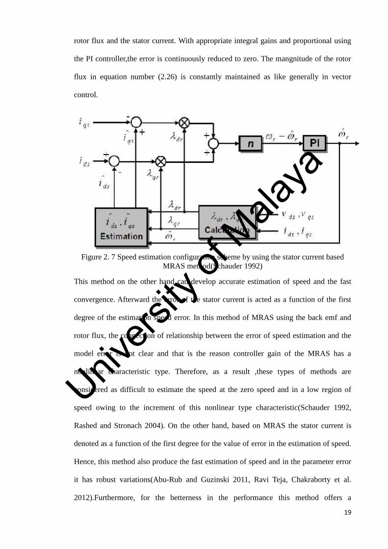
19
rotor flux and the stator current. With appropriate integral gains and proportional using
the PI controller,the error is continuously reduced to zero. The mangnitude of the rotor
flux in equation number (2.26) is constantly maintained as like generally in vector
control.
Figure 2. 7 Speed estimation configuration scheme by using the stator current basedMRAS method(Schauder 1992)
This method on the other hand can develop accurate estimation of speed and the fast
convergence. Afterward the error of the stator current is acted as a function of the first
degree of the estimation speed error. In this method of MRAS using the back emf and
rotor flux, the connection of relationship between the error of speed estimation and the
model error is not clear and that is the reason controller gain of the MRAS has a
nonlinear characteristic type. Therefore, as a result ,these types of methods are
considered as difficult to estimate the speed at the zero speed and in a low region of
speed owing to the increment of this nonlinear type characteristic(Schauder 1992,
Rashed and Stronach 2004). On the other hand, based on MRAS the stator current is
denoted as a function of the first degree for the value of error in the estimation of speed.
Hence, this method also produce the fast estimation of speed and in the parameter error
it has robust variations(Abu-Rub and Guzinski 2011, Ravi Teja, Chakraborty et al.
2012).Furthermore, for the betterness in the performance this method offers a
Univers
ity of
Mala
ya
20
considerable improvements of the sensorless vector controller at the low
speed.Summary of MRAS method review is shown in the below table number 2.1.
Table 2. 1 Advantages and distadvantage of MRAS method
Advantages Drawbacks
Algorithms of MRAS are
robustness.
Main drawback of MRAS algorithm are their
sensitivity to inaccuracies in reference model.
Fast convergence.Designing of the adaption mechanism block have
a lot difficulties.
Small computation time.
Selection of the adaptive gains mechanism is
selection between achieving high robustness
against noise and fast response and the
disturbance effect the system in this case.
2.5 Kalman Filter approach
The system which has many unknown noises such as; ripple in the current by PWM,
noise by the modelling error, error in measurement and so forth for that system the
algorithm of Kalman Filter (KF) is suitable and all these errors are treated as
disturbance in this algorithm method. In real type of system, some uncertainties in the
environment and model as disturbances, as modelling inaccuracies and noises should be
considered (Al-Tayie and Acarnley 1997, da Silva and Kankam 1997, Garcia Soto,
Mendes et al. 1999, Khalil, Strangas et al. 2009). With random noises the state
equations can be expressed as;
( ) = Ax(t) + Bu(t) + G(t) (2.27)
y(t) = Cx(t) + v(t) (2.28)
Univers
ity of
Mala
ya

21
Where, x(t) is the state variable, u(t) is the commands variables, and y(t)is the output
variables. However, G(t) and v(t) are the input and output noises respectively.
The KF method is not purely applicable for the nonliear problems,whereas the linearity
plays a significant role in its performance as an optimal filter and in its derivation.
Undertakes of the extended kalman filter (EKF) method by using the linearized
approximation, the attempts to get over this kind of the difficulty where the linearization
is performed for the current estimate state. Discretization of equation (2.27) and (2.28)
is required for this process as;
x(k + 1) = A(k)x(k) + B(k)u(k) + G(k) (2.29)
y(k) = C(k)x(k) + v(k)(2.30)
Algorithm of Kalman filter is expressed as;
P(0) = Var{X(0)} (2.31)
X(0) = E{X(0)} (2.32)
P(K + 1) = A(K)P(k)A (K) + Q (2.33)
X(K + 1) = A(K)X(K) + B(K)u(K) (2.34)
K(K + 1) = P(K + 1)C (K)[C(K)P(K + 1)C (K) + R]-1 (2.35)
X(K + 1/K) = X (K + 1) + K(K + 1) y(K) − C(K) X(K + 1) (2.36)
Where;
K(k+1) = the Kalman gain matrix.
Var(x) = the variance of x.
P(k) = error covariance matrix.
E(x) = the expectation of x.
Univers
ity of
Mala
ya
22
y(k) = the estimated output.
The matrix R shows the noise developed by transforming the estimated output into
sampled data model, and Q is the disturbances here such as the error which produced by
transforming into the sampled one data of the system. Approach structure of the kalman
filter is typically shown in figure number 2.8. Due to modelling error and imperfection
of the current controller the error is produced.
Figure 2. 8 Kalman filter structure for estimation of speed(Khalil, Strangas et al. 2009)
The inputs to the plant are fed into a prediction type model, and the output of that plant
is equated with the output from the model. The resulting error which comes after being
compared is fed into a kalman gain correction stage for the purpose of reducing the
error in the estimated states from that prediction model. The approach of this method of
kalman filter has some inherent type of disadvantages such like; the absence of the
tuning criteria and design, and the influence of computation burden. As well, it is
comparatively difficult to analyse and required much more powerful type
microprocessors.
2.6. Artificial intelligence techniques
Control of the non linear dynamic systems and to identify the use of Artificial
Intelligence (AI) has been suggested. Reason is that they can guess a wide range
Univers
ity of
Mala
ya
23
function of nonlinear to any wanted accuracy of degree. Furthermore, Artificial
Intelligence (AI) has the advantages of the exemption from ripples of input harmonics
and the robustness to the variations of parameters. Latterly, there have been many
researches, investigations into the application of Artificial Intelligence to the IM drives,
the power electronics, and also including the estimation of the speed(Campbell and
Sumner 2002, Lopez, Romeral et al. 2006, Rafiq, Habibullah et al. 2012, Sedhuraman,
Himavathi et al. 2012). AI’s two applications are used in research for induction motor in
which neural network (ANNs) model and Fuzzy logic control (FLC) based model are in
research area field.
2.6.1 Neural Network based model
Using NN model with the two well-known current and voltage model are necessary for
estimating the speed of an induction motor, because the voltages and the currents of the
induction motor are calculated in the stationary reference frame which is very much
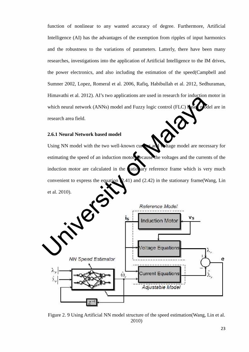
convenient to express the equation (2.41) and (2.42) in the stationary frame(Wang, Lin
et al. 2010).
Figure 2. 9 Using Artificial NN model structure of the speed estimation(Wang, Lin et al.2010)
Univers
ity of
Mala
ya
24
Illustration of the method using NN model and also the equations (2.41) and (2.42) are
defined in the figure number 2.9. Equations are expressed as follows (Seong-Hwan,
Tae-Sik et al. 2001);
= − + 00 + (2.41)
= − + (2.42)
Reference model is defined by the voltage equations that don’t involve and defining
the current equation with method of adjustable model by the involvement of .The
estimated speed is defined as the output of the ANNs, which afterwards is used as the
input of the adjustable model. The error occurs between the flux from the reference
model and the flux from the adjustable model when the estimated speed deviates
from the real speed. Subsequently that error is back-propagated to the model AAN and
the weights of model NN are adjusted online to decrease the error. Eventually, the
output of the model NN pursues the real speed. Though methods which are based on
ANN also give the good speed estimation along with parameters mismatch, however
they are in truth, they are comparatively very complicated and needs large time for
computation.
2.6.2 Fuzzy logic based model
In the existing research area literature on fuzzy logic control there are two most popular
methods reviewed, the Mamdani and Sugeno systems. Both of these methods are
characterised by the logics rules “IF-THEN” and in nature have the same antecedent
type structure. Nevertheless, there is difference between them in the structure of the
consequent parts. The consequent of the method based on Sugeno rule is nonlinear or
linear type function of the inputs variables, whereas comparatively with the consequent
Univers
ity of
Mala
ya
25
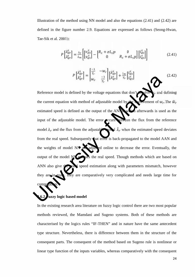
of a Mamdani based rule is a fuzzy type set(Venkataramana Naik and Singh 2012).The
development of the structure is for both such as type-1 fuzzy logic control (TP1FLC)
which reduced order and type-2 fuzzy logic control (TP2FLC) as shown in the figure
number 2.10, as the fuzzification and de-fuzzification procedure is quite remain same
as type-1 fuzzy logic control (TP1FLC)(Qilian and Mendel 2000).
Figure 2. 10 type-2 Fuzzy logic Control(Venkataramana Naik and Singh 2012)
It has been observed also from research review papers by using the PI fuzzy controller
that the oscillation has been not only cancelled but the speed profile became the
smoother as well(Abdalla, Hairik et al. 2010). The PI controller with fuzzy logic scheme
for the direct control of the torque is shown in the figure number (2.11); the main
feature of this scheme is the fuzzy self adaptation PI control block.
Univers
ity of
Mala
ya
26
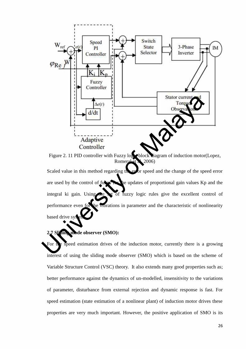
Figure 2. 11 PID controller with Fuzzy logic block diagram of induction motor(Lopez,Romeral et al. 2006)
Scaled value in this method regarding the error speed and the change of the speed error
are used by the control of fuzzy for the updates of proportional gain values Kp and the
integral ki gain. Using the set of fuzzy logic rules give the excellent control of
performance even for the vibrations in parameter and the characteristic of nonlinearity
based drive system.
2.7 Sliding mode observer (SMO):
For the speed estimation drives of the induction motor, currently there is a growing
interest of using the sliding mode observer (SMO) which is based on the scheme of
Variable Structure Control (VSC) theory. It also extends many good properties such as;
better performance against the dynamics of un-modelled, insensitivity to the variations
of parameter, disturbance from external rejection and dynamic response is fast. For
speed estimation (state estimation of a nonlinear plant) of induction motor drives these
properties are very much important. However, the positive application of SMO is its
Univers
ity of
Mala
ya

27
application for estimation of speed in induction motor drives which requires the
elimination of chattering problem (Derdiyok 2005, Jingchuan, Longya et al. 2005,
Edelbaher, Jezernik et al. 2006, Khater, Zaky et al. 2006, Lascu and Andreescu 2006).
Representation of induction motor is by its own dynamic model which is expressed in
the reference stationary frame in terms of the rotor flux and stator current as by the
following state equations.
iλ = a aa a iλ + b0 [U ] = AX + Bu(2.43)
Whereas,
a = aI,a = cI + dJ,a = eI,a = −ԑa ,
b = bI,Estimation of the rotor flux the SMO can be built as;
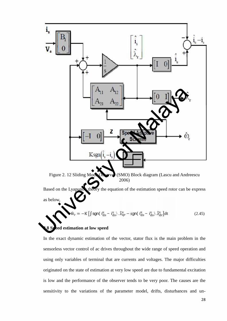
= + Bu + K sgn(ı − i ) (2.44)
Where the K is a matrix gain which is arranged as below, and the structure of the SMO
regarding speed estimation algorithm is shown in Fig. 2.12.
K = [K −K]T,
K = KI,K is switching gain.
Univers
ity of
Mala
ya
28
Figure 2. 12 Sliding Mode Observer (SMO) Block diagram (Lascu and Andreescu2006)
Based on the Lyapunov theory the equation of the estimation speed rotor can be express
as below,
w = −K ∫ sgn( ı − i ) . λ − sgn( ı − i ). λ dt (2.45)
2.8 Speed estimation at low speed
In the exact dynamic estimation of the vector, stator flux is the main problem in the
sensorless vector control of ac drives throughout the wide range of speed operation and
using only variables of terminal that are currents and voltages. The major difficulties
originated on the state of estimation at very low speed are due to fundamental excitation
is low and the performance of the observer tends to be very poor. The causes are the
sensitivity to the variations of the parameter model, drifts, disturbances and un-
Univers
ity of
Mala
ya
29
modelled nonlinearities, limitation in accuracy of acquisition signals and dc offsets. The
main three sources of the poor estimation of speed are as Data Acquisition Errors,
Voltage Distortion due the PWM Inverter and Stator Resistance Drop(Tajima, Guidi et
al. 2000, Holtz 2002, Holtz and Juntao 2003, Consoli, Scarcella et al. 2004).
2.8.1 Data Acquisition Errors
Data Acquisition Errors turns to substantial at low speeds. Reason for that are the
current sensors converts the currents of the machine in to the voltage signals which are
afterwards digitised through A/D converters. Dc offset component specially the
parasitic are superimposed on top to the analogue signals and appear as ac components
which belongs to fundamental frequency right after their transformation to the
synchronous type coordinates. For the current controller they act as disturbances. That’s
why torque ripple generates and there is also another problem in it which is the effect of
unbalanced gains of the current acquisition channels(Holtz 2002).
2.8.2 Voltage Distortion due the Pulse Width Modulation (PWM) Inverter
Usage of Pulse Width Modulation (PWM) controlled switches is the task to produce the
desired voltage on the stator winding by the power inverter. Afterwards the time of the
switching of the existing transistor is not infinitely short. During the commutations, the
knowledge about the necessary blanking time must brought which avoid short circuiting
the dc link which is known as “dead time” also. The importance of small time is
because of that inverter nonlinearity also introduces a phase error in the output-voltage
vector and a magnitude.
In the addition of the dead time across the switch during the ON State there is voltage
drop also at finite level which is the reason of introducing an extra, also called
additional error in the magnitude of the voltage at output. Taking in consideration,
regarding inverter model enables the more estimation of vector stator flux linkage speed
Univers
ity of
Mala
ya
30
accurate and accordingly, better speed estimated is achieved(Holtz 2002, Holtz and
Juntao 2002).
2.8.3 Stator Resistance Drop
Compared with the stator voltage the resistive drop of voltage is small in the upper
speed range. That’s the reason the speed estimation and the stator flux vector can be
made with better accuracy, frequency of stator is also low at the low speeds. Voltage of
the stator reduces in direct proportion almost, while at low speed it becomes significant
and the resistive drop voltage maintains its magnitude order. Speed estimation is
because of the great influence on the estimation accuracy of the flux stator vector due to
the resistive voltage drop. On other way, the vibrations of the resistance of the stator
which takes in considerable variations are found when the temperature of machine
changes at the varying load. These variations are supposed to be tracked which are
necessary to maintain the stability of the flux estimation at the low speed (Holtz 2002,
Holtz and Juntao 2003). Several methods for improving the performance of the voltage
model at low frequency have been proposed. For instance, accurate measurements for
the stator current and voltage, compensation of the voltage drop due to inverter, and the
resistance of the stator also can be identified with an adaptive scheme(Holtz and Juntao
2002, Holtz and Juntao 2003).
2.9 Parameter Adaption
In spite of the facts referred from reviewed research, the method based on machine
model for the estimation of the speed are characterised due to their simplicity.
Sensitivity due to variations in parameter is one of the problems associated also with
them. Resistance region in the low speed of the stator plays an important role, and value
of resistance should be known with the good precision in order to achieve the accurate
estimation of the rotor speed(Zamora and Garcia-Cerrada 2000, Vasic, Vukosavic et al.
Univers
ity of
Mala
ya
31
2003). Heating of the motor usually is the reason of vibration in the winding resistance
which is considerable. Afterwards it becomes the causes of the mismatch between the
actual resistance of the winding and its corresponding value in the model system which
is used for the estimation of the speed. This might lead not only to a large error
estimation of speed but also the instability occur as well, and recently the consequence
for that the numerous online schemes for the resistance of stator recognition have been
proposed (Zamora and Garcia-Cerrada 2000, Vasic, Vukosavic et al. 2003).
Identification availability of online resistance of stator schemes can be sorted into a
couple of clear cut categories. Reliability of all these methods is on the measurements of
the stator current and primarily there is requirement of the information regarding
voltage of the stator as well (Vasic, Vukosavic et al. 2003, Edelbaher, Jezernik et al.
2006). To update the value of stator resistance, the most famous method includes the
different kinds of estimators which frequently use an adaptive mechanism (Vasic,
Vukosavic et al. 2003, Edelbaher, Jezernik et al. 2006). Stator resistance is supposed to
be determined through reactive power which is based on model reference adaptive
system (MRAS) (Edelbaher, Jezernik et al. 2006). The reliability of the reactive power
is on the accuracy of other parameters such as rotor resistance which are not necessarily
constant and reason as results is prone to error. Another reliability of reactive power is
on leakage inductance. For the estimation of the speed and the resistance of the stator,
there is method of Adaptive full order flux observers (AFFO) which are developed with
the help of using Popov’s and Lyapunov stability criteria(Hossein Madadi Kojabadia
2005, Wang, Lin et al. 2010). With regard to computation while these types of schemes
are not intensive and might AFFO with matrix non zero gain become unstable. For
speed estimation and the resistance of the stator with the help of using the model
reference adaptive system which is developed with the help of using stability criterion
of Popov’s (Vasic, Vukosavic et al. 2003, kojabadi 2005). With the difference between
Univers
ity of
Mala
ya
32
two types of stator currents which is measured and the observed stator current, in this
method mechanism of stator resistance adaption can be determined.
Need of the wide speed range which could have maximum required speed, which means
considerably exceeds the speed of the motor’s rated speed are required for the
application such as gearless traction drives and spindle. Redoubtable difficulties occur
during speed estimation in the field weakening region regardless of the method used for
the estimation of speed. In the region of field weakening the model which have
approaches on AC machines, considered as the main problem which have roots from the
fairly large variation of magnetizing inductance as the main saturation of flux which is
neglected in estimation of speed based model. Hence, the exact estimation of speed is
possible in the weakening field region using the approach of model based. If and only
modifying the algorithm of the speed estimation in such way in which the variation of
the main flux saturation is made out within the estimator (Myoung-Ho and Dong-Seok
2003, Tae-Sung, Myoung-Ho et al. 2005). In the speed base region, the induction motor
of a field oriented operates with reference of rated rotor flux which is constant. Hence,
as result the magnetizing inductance can be considered as equal to its value of rated and
as constant also. At higher speeds the operation in the weakening field region compare
to rated speeds causes that the flux of the rotor reference has to be diluted below the
value of rated speeds. The variation of the flux of rotor reference in the machine implies
the variable level of the main flux saturation and accordingly the variable parameter of
the machine is the magnetizing inductance (Levi and Mingyu 2002, Levi and Mingyu
2003).Value of magnetizing inductance especially the accurate one is extremely
important for many reasons. First one, the correct setting of the d-axis reference current
of stator in a drive of vector controlled which needs the precise value magnetizing
inductance to be known. Second one, the accurate estimation of the speed using the
model based machine’s approaches for the procedure in the field region weakening.
Univers
ity of
Mala
ya

33
Third reason, is the dependency of constant time of rotor which is identification
schemes on magnetizing of inductance such as the process in which utilize the method
of reactive power(Levi and Mingyu 2002). Correct value of the magnetizing inductance
is required to be known for the estimation of accurate constant time of rotor in the field
of weakening region.
In the area of research, many are committed on this and giving the way to better speed
estimation in the weakening field oriented type control of induction motor which is in
constant flux region operation. Nevertheless, the analyses on the inductance of
magnetising identification regarding the improvement of the speed estimation in the
field of weakening region are still seldom made (Huang and Liaw 2003). In the state of
transient and steady state the better dynamic response can get by the representation of
the fitted quadratic polynomial of the current field for the nonlinear magnetizing
inductance. Magnetizing inductance identification method is employed on which
measured voltage of stator and currents depends and also the magnetizing curve of the
machine(Levi and Mingyu 2003).
2.10 Adaptive flux observer (AFO)
For the purpose of speed estimation of induction motor drives the Adaptive Flux
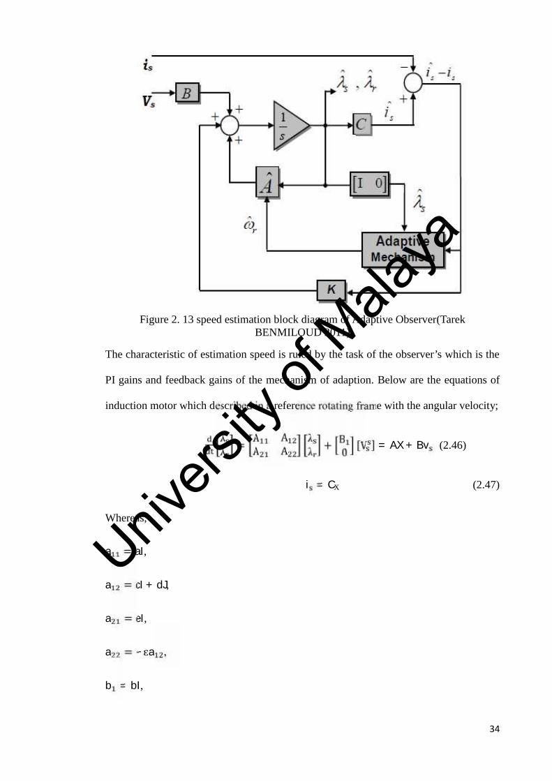
observers are also used. The construction of the adaptive observer is essentially framed
in three types of main parts: Model of the induction motor, feedback gains of the
observer, and mechanism of adaption regarding rotor speed as shown in the figure 2.13.Univers
ity of
Mala
ya
34
Figure 2. 13 speed estimation block diagram of Adaptive Observer(TarekBENMILOUD 2011)
The characteristic of estimation speed is ruled by the task of the observer’s which is the
PI gains and feedback gains of the mechanism of adaption. Below are the equations of
induction motor which described in a reference rotating frame with the angular velocity;
λλ = A AA A λλ + B0 [V ] = AX + Bv (2.46)
i = CX (2.47)
Whereas,
a = aI,a = cI + dJ,a = eI,a = −ԑa ,
b = bI,
Univers
ity of
Mala
ya
35
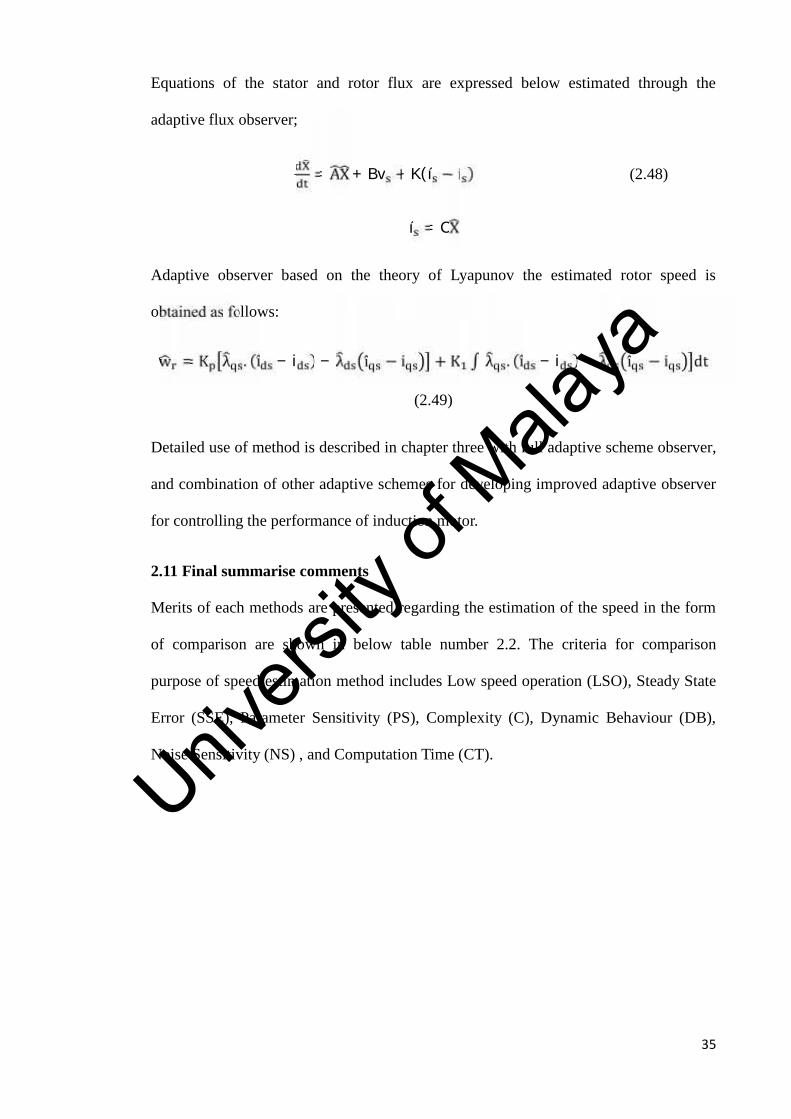
Equations of the stator and rotor flux are expressed below estimated through the
adaptive flux observer;
= AX + Bv + K(ı − i ) (2.48)
ı = CXAdaptive observer based on the theory of Lyapunov the estimated rotor speed is
obtained as follows:
w = K λ . (ı − i ) − λ ı − i + K ∫ λ . (ı − i ) − λ ı − i dt(2.49)
Detailed use of method is described in chapter three with full adaptive scheme observer,
and combination of other adaptive schemes for developing improved adaptive observer
for controlling the performance of induction motor.
2.11 Final summarise comments
Merits of each methods are presented regarding the estimation of the speed in the form
of comparison are shown in below table number 2.2. The criteria for comparison
purpose of speed estimation method includes Low speed operation (LSO), Steady State
Error (SSE), Parameter Sensitivity (PS), Complexity (C), Dynamic Behaviour (DB),
Noise Sensitivity (NS) , and Computation Time (CT).
Univers
ity of
Mala
ya

36
Table 2. 2 Comparison of different methods regarding estimation speedMethod/Criteria CT C NS PS LSO DB SSE
FSI 3 5 4 1 1 2 2
RST 3 5 4 1 1 2 2
MMM
SM 2 2 2 1 2 1 1
AI 4 3 2 1 2 1 1
AFO 2 2 2 3 3 1 2
KF 5 5 1 2 2 2 2
MRAS 3 2 4 3 4 3 2
DCM 2 2 4 4 4 3 2
Grading of merit based ranges is from 1 to 5 in the table 2.2, where (1) indicates “the
best behaviour” whereas (5) indicates “the weakest one” as shown in the table number
2.3.
Note all the comparison is based on the comprehensive study and the investigation of
the literature review.
Table 2. 3 Grading on merit based of speed estimationBest Very Good Good Satisfactory Weak
1 2 3 4 5
According to the adopted set of criteria comparison of different speed estimation is
shown in the form of chart based on above table of grading in figure number 2.14.
Univers
ity of
Mala
ya
37
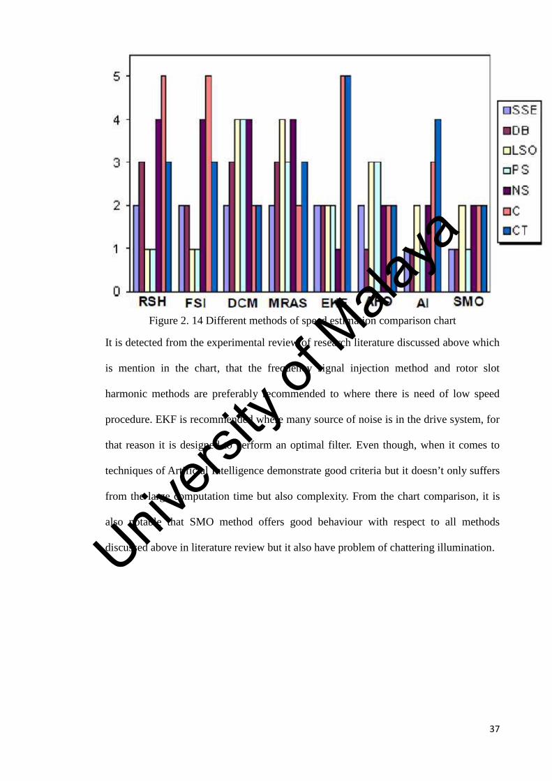
Figure 2. 14 Different methods of speed estimation comparison chart
It is detected from the experimental review of research literature discussed above which
is mention in the chart, that the frequency signal injection method and rotor slot
harmonic methods are preferably recommended to where there is need of low speed
procedure. EKF is recommended where many source of noise is in the drive system, for
that reason it is designed to perform an optimal filter. Even though, when it comes to
techniques of Artificial Intelligence demonstrate good criteria but it doesn’t only suffers
from the large computation time but also complexity. From the chart comparison, it is
also notable that SMO method offers good behaviour with respect to all methods
discussed above in literature review but it also have problem of chattering illumination.Univers
ity of
Mala
ya
38
CHAPTER THREE: METHODOLOGY
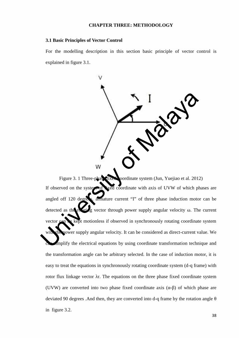
3.1 Basic Principles of Vector Control
For the modelling description in this section basic principle of vector control is
explained in figure 3.1.
Figure 3. 1 Three-phase fixed coordinate system (Jun, Yuejiao et al. 2012)
If observed on the system of fixed coordinate with axis of UVW of which phases are
angled off 120 degrees, armature current “I” of three phase induction motor can be
detected as the rotating vector through power supply angular velocity ω. The current
vector can be kept motionless if observed in synchronously rotating coordinate system
with the power supply angular velocity. It can be considered as direct-current value. We
can simplify the electrical equations by using coordinate transformation technique and
the transformation angle can be arbitrary selected. In the case of induction motor, it is
easy to treat the equations in synchronously rotating coordinate system (d-q frame) with
rotor flux linkage vector λr. The equations on the three phase fixed coordinate system
(UVW) are converted into two phase fixed coordinate axis (α-β) of which phase are
deviated 90 degrees .And then, they are converted into d-q frame by the rotation angle θ
in figure 3.2.
Univers
ity of
Mala
ya
39
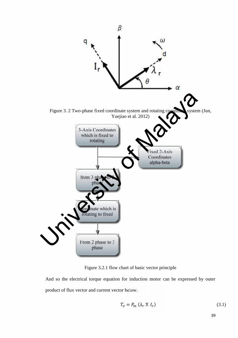
Figure 3. 2 Two-phase fixed coordinate system and rotating coordinate system (Jun,Yuejiao et al. 2012)
Figure 3.2.1 flow chart of basic vector principle
And so the electrical torque equation for induction motor can be expressed by outer
product of flux vector and current vector below.
= ( X ) (3.1)
Univers
ity of
Mala
ya

40
Where,
: Number of poles pares.
: Rotor flux vector [ ]T
: Rotor current vector [ ]T
Therefore equation 3.1 also can be modified by treating the d axis as rotor flux vector.
= − = ( ) (3.2)
Where,
M: Coefficient of mutual induction.
: Self induction of rotor.
With the constant rotor flux of equation 3.2, the torque of the motor can also be
controlled by q-axis current of stator. Therefore, the flux of rotor can be expressed as;
= (3.3)
Where,
Time constant: =The above equation shows that by the d - axis current of stator, the flux of the rotor can
be controlled to be constant. Using the constant target value of current in the similar
way as traditional DC brush motor allows controlling the motor torque in coordinate
conversion by phase of flux vector.
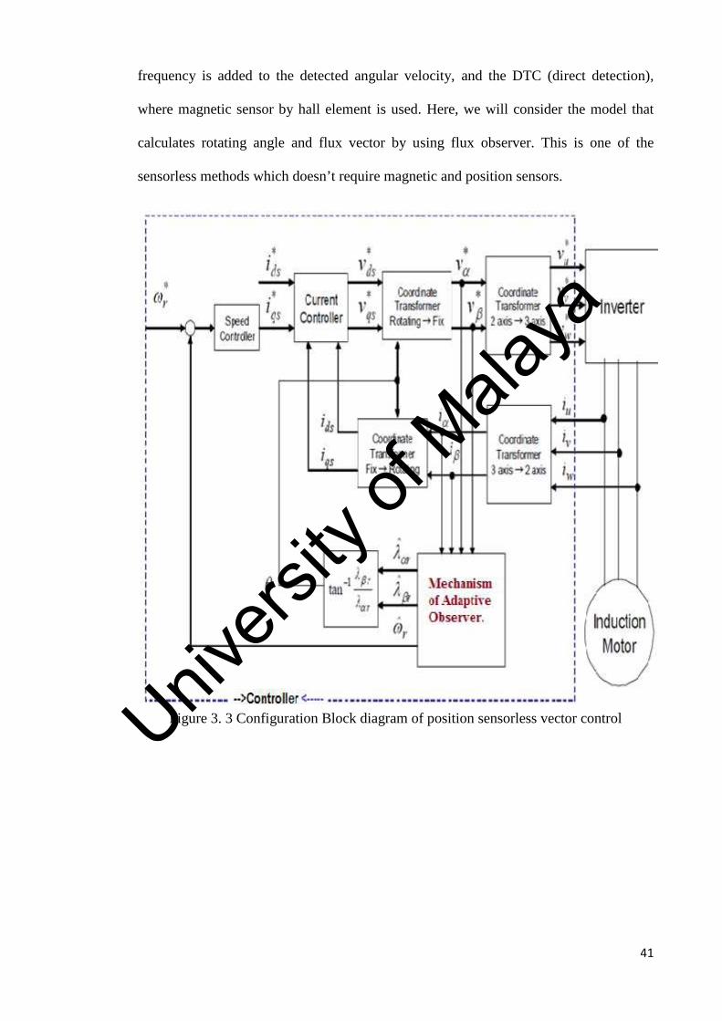
3.2 System Modelling
An accurate flux vector is very important to determine in induction motor. Detection of
flux vector includes some methods such as; indirect detection, where slip angular
Univers
ity of
Mala
ya
41
frequency is added to the detected angular velocity, and the DTC (direct detection),
where magnetic sensor by hall element is used. Here, we will consider the model that
calculates rotating angle and flux vector by using flux observer. This is one of the
sensorless methods which doesn’t require magnetic and position sensors.
Figure 3. 3 Configuration Block diagram of position sensorless vector controlUnivers
ity of
Mala
ya

42
3.2.1. Description of Symbols
Self-inductance [H] L
Resistor [Ω] R
Laplace operator S
number of pole pairs Pm
current value [A] I
Flux linkage Λ
Electric torque [Nm] Te
Rotor flux angle velocity [rad/sec] Ω
voltage value [V] V
Electric angular velocity [rad/sec] Ωr
Rotor flux rotation angle [rad] Θ
mutual inductance [H] M
3.2.2 Subscript symbol description
Estimation value ^
Variables in three-phase fixed coordinate
systemU, V, W
Variable in the rotor R
Variables in orthogonal two-axis fixed
coordinate systemα,β
Target value *
Variables in orthogonal two-axis rotating
coordinate systemd, q
Variable in the stator S
Univers
ity of
Mala
ya
43
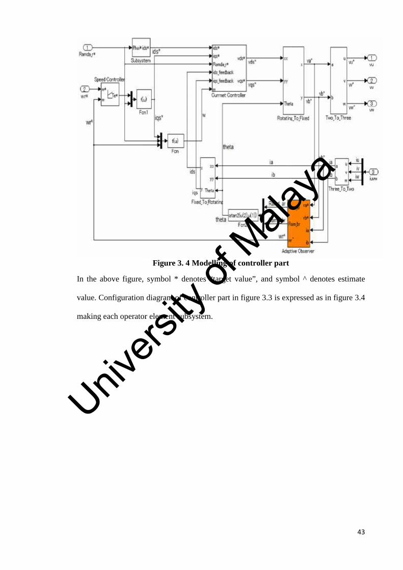
Figure 3. 4 Modelling of controller part
In the above figure, symbol * denotes “target value”, and symbol ^ denotes estimate
value. Configuration diagram of controller part in figure 3.3 is expressed as in figure 3.4
making each operator element subsystem.
43
Figure 3. 4 Modelling of controller part
In the above figure, symbol * denotes “target value”, and symbol ^ denotes estimate
value. Configuration diagram of controller part in figure 3.3 is expressed as in figure 3.4
making each operator element subsystem.
43
Figure 3. 4 Modelling of controller part
In the above figure, symbol * denotes “target value”, and symbol ^ denotes estimate
value. Configuration diagram of controller part in figure 3.3 is expressed as in figure 3.4
making each operator element subsystem.
Univers
ity of
Mala
ya

44
3.2.3 Description of signal label
Subscript indicating target value *
Voltage target values on α, β axes va, vb
Current values on α and βaxes ia, ib
Thetapower supply angle - Rotor flux rotation
angle
Current value on UVW axis iu, iv, iw
Voltage target values on UVW axis vu, vv, vw
Voltage target value on d and q axes vds, vqs
Current target values on d and q axes ids, iqs
Rotor flux rotating angler velocity (power
supply angler velocity)W
Electric angler velocity estimation value Wr
Rotor flux of α and β axes Ramd_ar, Ramd_br
Univers
ity of
Mala
ya

45
Below equation is the expression of coordinate transformation.Transformation Equation
From the coordinate which is fixed to
rotating.=
From the coordinate which is rotating to
fixed. =
Phases: from 3Φ to 2Φ =
Phases: from 2Φ to 3Φ =
Where,
Rotary matrix:
C = cos θ sin θ− sin θ cos θThree-phase to two-phase transformation matrix:
D = cos 0 cos ( ) cos ( )sin0 sin( ) sin( )Where,
_ Denotes vector
e Denotes direct-current value
Univers
ity of
Mala
ya
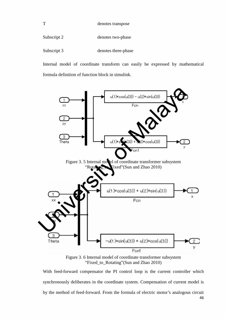
46
T denotes transpose
Subscript 2 denotes two-phase
Subscript 3 denotes three-phase
Internal model of coordinate transform can easily be expressed by mathematical
formula definition of function block in simulink.
Figure 3. 5 Internal model of coordinate transformer subsystem“Rotating_to_Fixed”(Sun and Zhao 2010)
Figure 3. 6 Internal model of coordinate transformer subsystem“Fixed_to_Rotating”(Sun and Zhao 2010)
With feed-forward compensator the PI control loop is the current controller which
synchronously deliberates in the coordinate system. Compensation of current model is
by the method of feed-forward. From the formula of electric motor’s analogous circuit46
T denotes transpose
Subscript 2 denotes two-phase
Subscript 3 denotes three-phase
Internal model of coordinate transform can easily be expressed by mathematical
formula definition of function block in simulink.
Figure 3. 5 Internal model of coordinate transformer subsystem“Rotating_to_Fixed”(Sun and Zhao 2010)
Figure 3. 6 Internal model of coordinate transformer subsystem“Fixed_to_Rotating”(Sun and Zhao 2010)
With feed-forward compensator the PI control loop is the current controller which
synchronously deliberates in the coordinate system. Compensation of current model is
by the method of feed-forward. From the formula of electric motor’s analogous circuit
Univers
ity of
Mala
ya
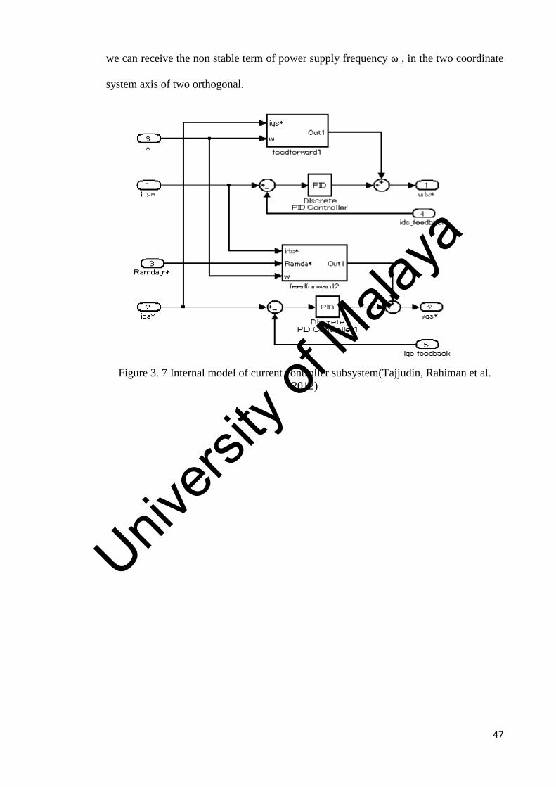
47
we can receive the non stable term of power supply frequency ω , in the two coordinate
system axis of two orthogonal.
Figure 3. 7 Internal model of current controller subsystem(Tajjudin, Rahiman et al.2012)
Univers
ity of
Mala
ya
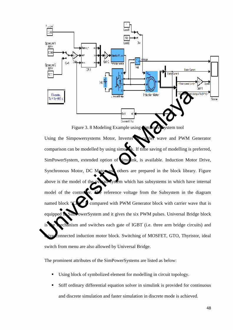
48
Figure 3. 8 Modeling Example using SimPowerSystem tool
Using the Simpowersystems Motor, Inverter of carrier wave and PWM Generator
comparison can be modelled by using simulink. If time saving of modelling is preferred,
SimPowerSystem, extended option of simulink, is available. Induction Motor Drive,
Synchronous Motor, DC Motor and others are prepared in the block library. Figure
above is the model of the overall system which has subsystems in which have internal
model of the controller. The reference voltage from the Subsystem in the diagram
named block “CPU” is compared with PWM Generator block with carrier wave that is
equipped in SimPowerSystem and it gives the six PWM pulses. Universal Bridge block
is the mechanism and switches each gate of IGBT (i.e. three arm bridge circuits) and
drive connected induction motor block. Switching of MOSFET, GTO, Thyristor, ideal
switch from menu are also allowed by Universal Bridge.
The prominent attributes of the SimPowerSystems are listed as below:
Using block of symbolized element for modelling in circuit topology.
Stiff ordinary differential equation solver in simulink is provided for continuous
and discrete simulation and faster simulation in discrete mode is achieved.
Univers
ity of
Mala
ya

49
Block inside almost can be referenced.
Automatic code generated tools are supported, RTW and real time-simulation is
accomplishable.
Many models as sample demo are available which are related to motor control
included vector control is provided which makes easy further development work
for sensorless control of motor.
3.3 Principles and Analysis Model Sensorless velocity by Adaptive Secondary Flux
Observer
If the same input voltage as actual voltage is applied to the mathematical simulator
model that is implemented on the processor, then Rotor flux should be estimated.
Nevertheless, when building the velocity sensorless system, changes of none stable
velocity term can not be formed by actual velocity sensor output and the calculated
value of flux will deviate from the actual value. Thus, by using the technique adaptive
observer that modifies the mathematical model of incorrect constant term with function
of the output deviation is applied. In this case, the electric angular velocity terms are
considered as the incorrect terms.
State-space formula of induction motor in orthogonal type two axis fixed coordinate
system can be expressed as below:
/ = + , = (3.4)
Where,
= [ ]T
= [ ]T
= [ ]T
Univers
ity of
Mala
ya

50
= 1 00 1 ,J= 0 −11 0
A = − (R + M R /L )(σL )I (R /ԑL )I − (ω /ԑ)J(MR /L )I − R L I + ω JB = I 0 T
C = [I 0 ]= 1 − M2( )
ԑ = σL L /MNote: reference: equation of basic vector control are applies.
Figure 3. 9 Adaptive Flux Observer Configuration Diagram (Savoia, Verrelli et al.2012)
For the above figure of observer, State-space expression can be expressed in the
equation below:
Univers
ity of
Mala
ya
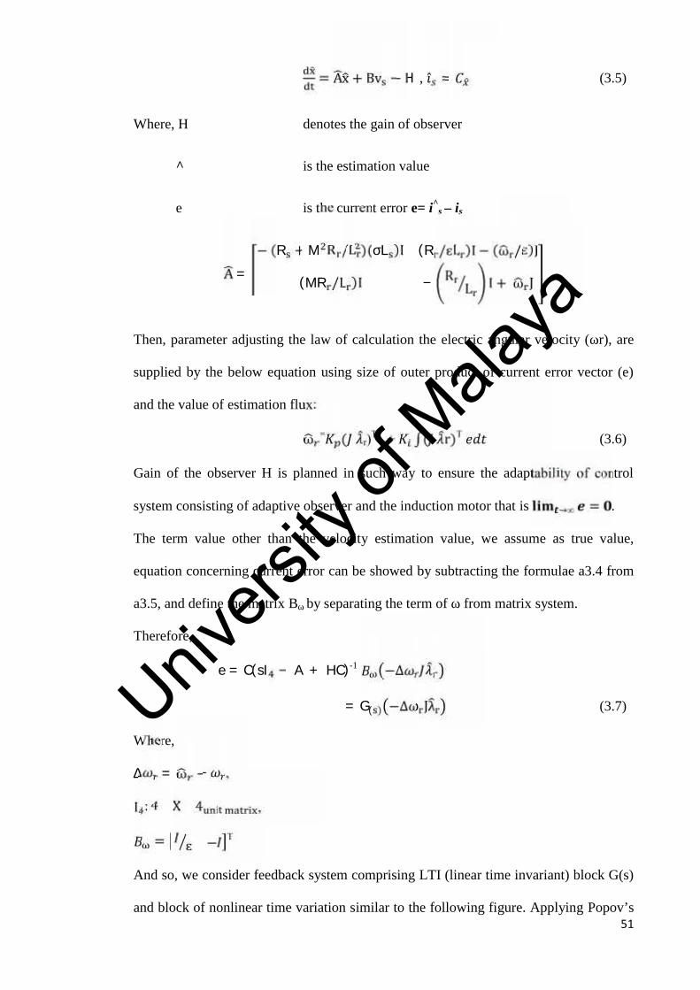
51
= Ax + Bv − H , = (3.5)
Where, H denotes the gain of observer
^ is the estimation value
e is the current error e= i^s – is
A = − (R + M R /L )(σL )I (R /ԑL )I − (ω /ԑ)J(MR /L )I − R L I + ω JThen, parameter adjusting the law of calculation the electric angular velocity (ωr), are
supplied by the below equation using size of outer product of current error vector (e)
and the value of estimation flux:ω = ( r)T
e + ∫( r)T (3.6)
Gain of the observer H is planned in such way to ensure the adaptability of control
system consisting of adaptive observer and the induction motor that is →∞ = .
The term value other than the velocity estimation value, we assume as true value,
equation concerning current error can be showed by subtracting the formulae a3.4 from
a3.5, and define the matrix Bω by separating the term of ω from matrix system.
Therefore, e = C(sI − A + HC)-1 −∆= G( ) −∆ω Jλ (3.7)
Where,∆ = ω − ,I : 4 X 4 ,= ԑ − T
And so, we consider feedback system comprising LTI (linear time invariant) block G(s)
and block of nonlinear time variation similar to the following figure. Applying Popov’s
Univers
ity of
Mala
ya

52
hyper stability, the below are necessary to be satisfied to ensure the stability →∞ =.
1. The Transfer function G(s) of feed forward LTI (Linear − Time − Invariant) isstrictly positive real (SPR).
2. Input v1 and the output w1 of non-linear time variation block satisfy the Popov’s
equation for all the time t1 greater than t0 (t1>t0).∫ > - (3.8)
Where,
: is constant independent of time.
Figure 3. 10 Current error block feedback system (Tarek BENMILOUD 2011)
The above figure is proved to be satisfied by using equation 3.6. Riccati equation is
applied for obtaining the optimal feedback gain to make G(s) SPR as a condition which
we mention above. H = PC R (3.9)
Univers
ity of
Mala
ya

53
Riccati equation: PA + AP − PC R CP + B QB = 0 (3.10)
Where,
P solution of Riccati equation
Q,R weight matrices
The weight matrices Q=1 and R=yI, respectively, however, y is a small positive
number.
3.4 Modeling of Adaptive observer
Program (M-file) of matlab language is used to set the all parameters of motor and each
matrix of state-space expression, and the formula 3.10 is solved with the help of using
the Control System Tool box , and we obtain the optimal feedback gain as well.
Where,
[H, P, E] = lqe(A, Bw, C, Q, R)
The function of Iqe is provided in Control System ToolBox for designing the Kalman
filter estimator and it returns the feedback gain, H, solution of Riccati equation, P, and
pole of estimator E= eig (A-H*C). M-file can be loaded in to the memory (workshop)
once executed in Matlab and define as each block parameter of Simulink model in it.
Adaptive observer subsystem in figure b is defined in figure (3.11) below.
Univers
ity of
Mala
ya
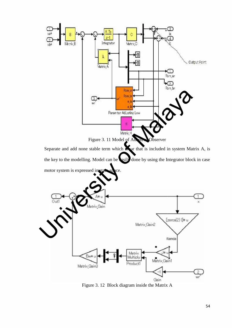
54
Figure 3. 11 Model of Adaptive Observer
Separate and add none stable term which is ωr that is included in system Matrix A, is
the key to the modelling. Model can be easily done by using the Integrator block in case
motor system is expressed in state-space.
Figure 3. 12 Block diagram inside the Matrix A
Univers
ity of
Mala
ya
55
Adaptive observer operates stably if the absolute value of the phase difference between
input and out is within 90 degrees. Subsequently it is verified the stableness of the
transfer function G(s) of linear stationary term. Linearization point is indicated as mark
of arrow below in the figure 3.11 is provided by simulink control design is located in
the relevant input and output points.
Hence, stability of transfer functions G(s) is verified. Adaptive observer operates stably
if the absolute value of phase difference between input and output is within 90 degrees.
Figure 3.13 is a bode diagram if linear time-invariant block G(s) drawn the LTI Viewer
of the Control System Toolbox. Referring to the phase diagram, you can see that weight
factor of formula (3.8) γ=1, γ=0.006, are within ±90° across the whole frequency range,
and they are stable.
Figure 3.13 Bode diagram of linear time-invariant block
Upper: gain characteristics Lower: phase characteristics, 0 mark line: γ=0.006, * mark
line: γ=1
Univers
ity of
Mala
ya
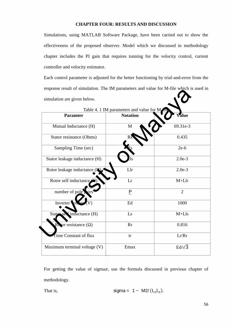
56
CHAPTER FOUR: RESULTS AND DISCUSSION
Simulations, using MATLAB Software Package, have been carried out to show the
effectiveness of the proposed observer. Model which we discussed in methodology
chapter includes the PI gain that requires tunning for the velocity control, current
controller and velocity estimator.
Each control parameter is adjusted for the better functioning by trial-and-error from the
response result of simulation. The IM parameters and value for M-file which is used in
simulation are given below.
Table 4. 1 IM parameters and value for M-fileParamter Notation Value
Mutual Inductance (H) M 69.31e-3
Stator resistance (Ohms) Rs 0.435
Sampling Time (sec) Ts 2e-6
Stator leakage inductance (H) Lls 2.0e-3
Rotor leakage inductance (H) Llr 2.0e-3
Rotor self inductance (H) Lr M+Llr
number of pole pairs P 2
Inverter voltage (V) Ed 1000
Stator self inductance (H) Ls M+Lls
Rotor resistance (Ω) Rr 0.816
Time Constant of flux tr Lr/Rr
Maximum terminal voltage (V) Emax Ed/√3For getting the value of sigma , use the formula discussed in previous chapter of
methodology.
That is, sigma = 1 − M2/(L L ).
Univers
ity of
Mala
ya

57
Value for the State Space Matrix: I = [1 0 : 0 1]J = [0 −1 : 1 0]Compute the variable for state space matrix value with the help of below formulas in M-
file.
A11 = − R + M ∗ RL(sigma ∗ L ) ∗ IA12 = M(sigma ∗ t ∗ L ∗ L ) ∗ I
A21 = Mt ∗ IA22 = − 1t ∗ I
Assigning the variables for memory to workspace variables of space vector:A = [A11 A12 : A21 A22]B = 1(sigma ∗ L ) ∗ I; zeros (2)
C = [I zeros(2)]Bw = [( ∗ ∗ )∗ ; −I]Value of weight matrix: ep = 0.006;R = ep ∗ I;Q = I;For obtaining the optima feed back gain, we can use the formula in M-file, discussed
previously in methodology.
[H, P, E] = lqe(A, Bw, C, Q, R)
Univers
ity of
Mala
ya
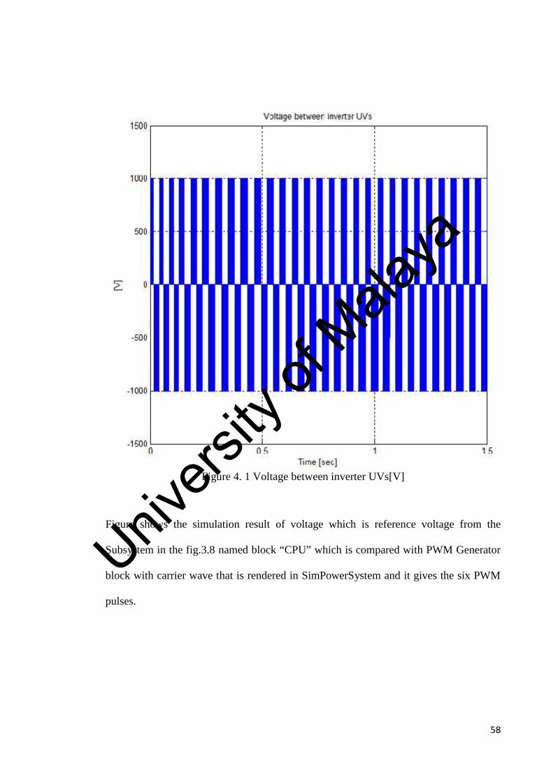
58
Figure 4. 1 Voltage between inverter UVs[V]
Figure shows the simulation result of voltage which is reference voltage from the
Subsystem in the fig.3.8 named block “CPU” which is compared with PWM Generator
block with carrier wave that is rendered in SimPowerSystem and it gives the six PWM
pulses.
Univers
ity of
Mala
ya
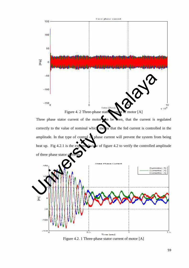
59
Figure 4. 2 Three-phase stator current of motor [A]
Three phase stator current of the motor can be seen, that the current is regulated
correctly to the value of nominal which means that the fed current is controlled in the
amplitude. In that type of control of phase current will prevent the system from being
heat up. Fig 4.2.1 is the expended view of figure 4.2 to verify the controlled amplitude
of three phase stator currents.
Figure 4.2. 1 Three-phase stator current of motor [A]
Univers
ity of
Mala
ya
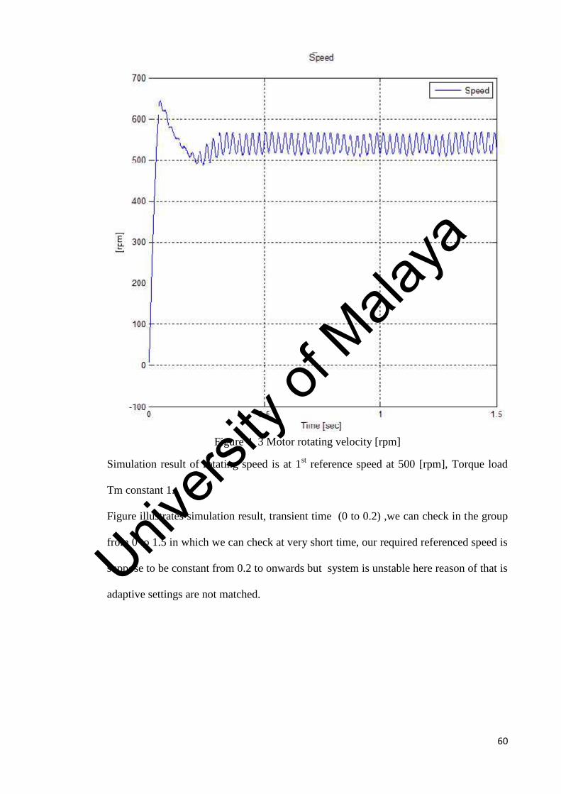
60
Figure 4. 3 Motor rotating velocity [rpm]
Simulation result of rotating speed is at 1st reference speed at 500 [rpm], Torque load
Tm constant 1.
Figure illustrates simulation result, transient time (0 to 0.2) ,we can check in the group
from 0 to 1.5 in which we can check at very short time, our required referenced speed is
suppose to be constant from 0.2 to onwards but system is unstable here reason of that is
adaptive settings are not matched.Univ
ersity
of M
alaya
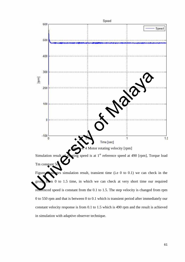
61
Figure 4. 4 Motor rotating velocity [rpm]
Simulation result of rotating speed is at 1st reference speed at 490 [rpm], Torque load
Tm constant 50.
Figure illustrates simulation result, transient time (i.e 0 to 0.1) we can check in the
group from 0 to 1.5 time, in which we can check at very short time our required
referenced speed is constant from the 0.1 to 1.5. The step velocity is changed from rpm
0 to 550 rpm and that is between 0 to 0.1 which is transient period after immediately our
constant velocity response is from 0.1 to 1.5 which is 490 rpm and the result is achieved
in simulation with adaptive observer technique.
Univers
ity of
Mala
ya
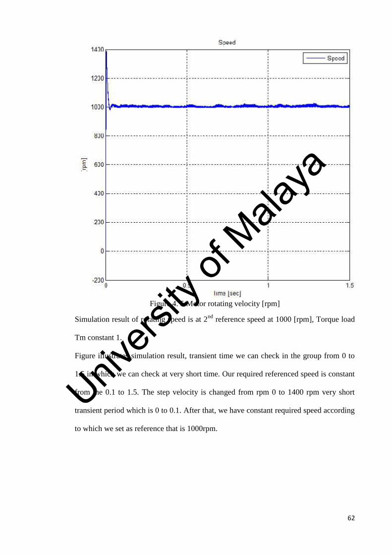
62
Figure 4. 5 Motor rotating velocity [rpm]
Simulation result of rotating speed is at 2nd reference speed at 1000 [rpm], Torque load
Tm constant 1.
Figure illustrates simulation result, transient time we can check in the group from 0 to
1.5 in which we can check at very short time. Our required referenced speed is constant
from the 0.1 to 1.5. The step velocity is changed from rpm 0 to 1400 rpm very short
transient period which is 0 to 0.1. After that, we have constant required speed according
to which we set as reference that is 1000rpm.
Univers
ity of
Mala
ya
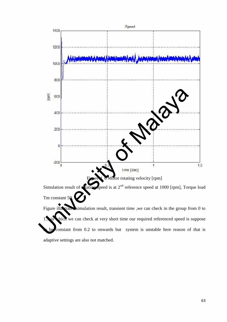
63
Figure 4. 6 Motor rotating velocity [rpm]
Simulation result of rotating speed is at 2nd reference speed at 1000 [rpm], Torque load
Tm constant 50.
Figure illustrates simulation result, transient time ,we can check in the group from 0 to
1.5 in which we can check at very short time our required referenced speed is suppose
to be constant from 0.2 to onwards but system is unstable here reason of that is
adaptive settings are also not matched.Univ
ersity
of M
alaya
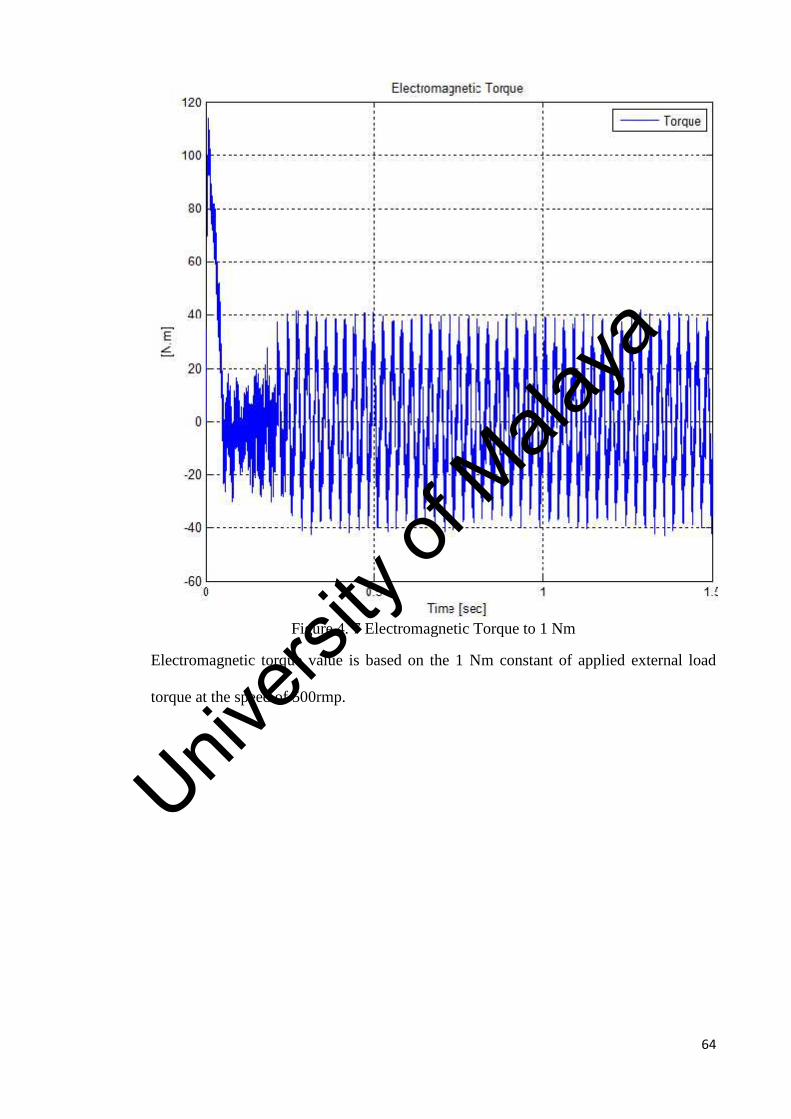
64
Figure 4. 7 Electromagnetic Torque to 1 Nm
Electromagnetic torque value is based on the 1 Nm constant of applied external load
torque at the speed of 500rmp.
Univers
ity of
Mala
ya
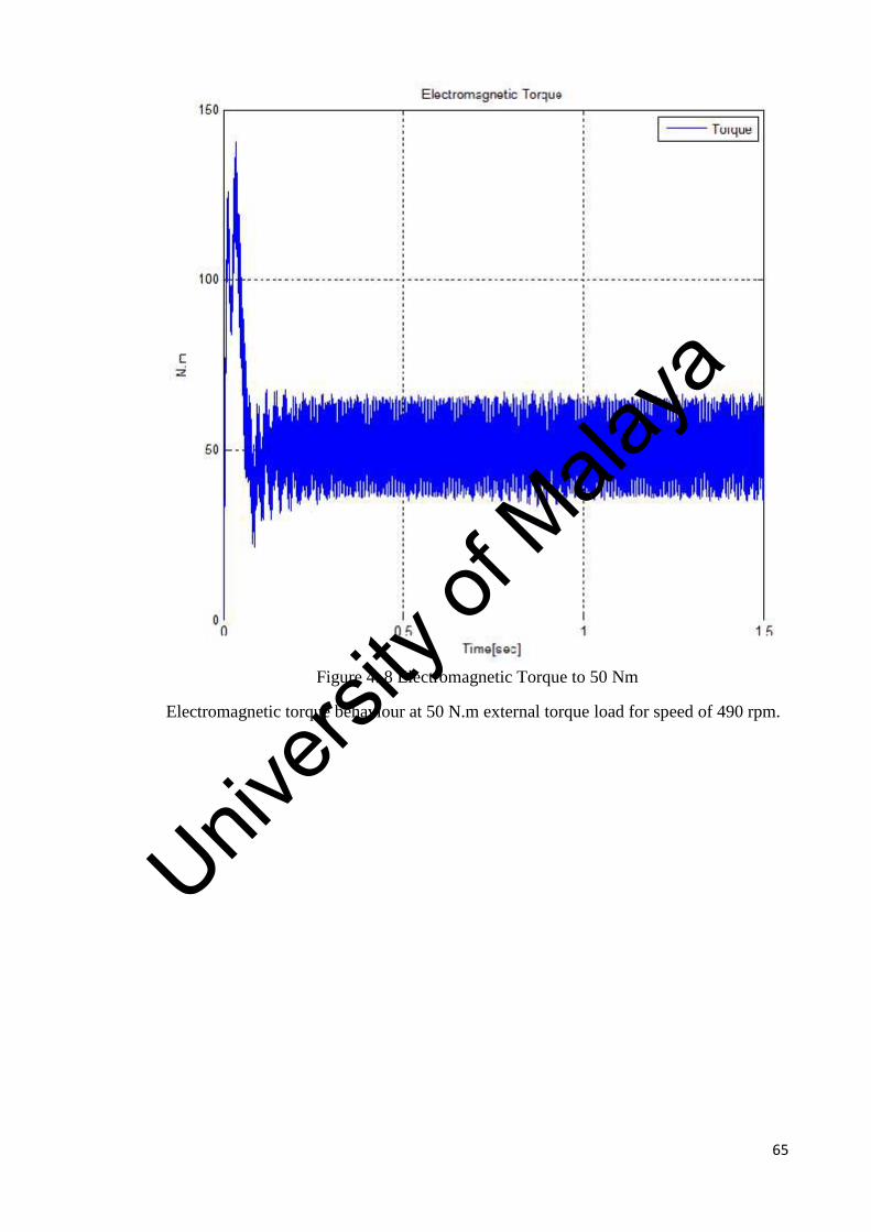
65
Figure 4. 8 Electromagnetic Torque to 50 Nm
Electromagnetic torque behaviour at 50 N.m external torque load for speed of 490 rpm.
Univers
ity of
Mala
ya
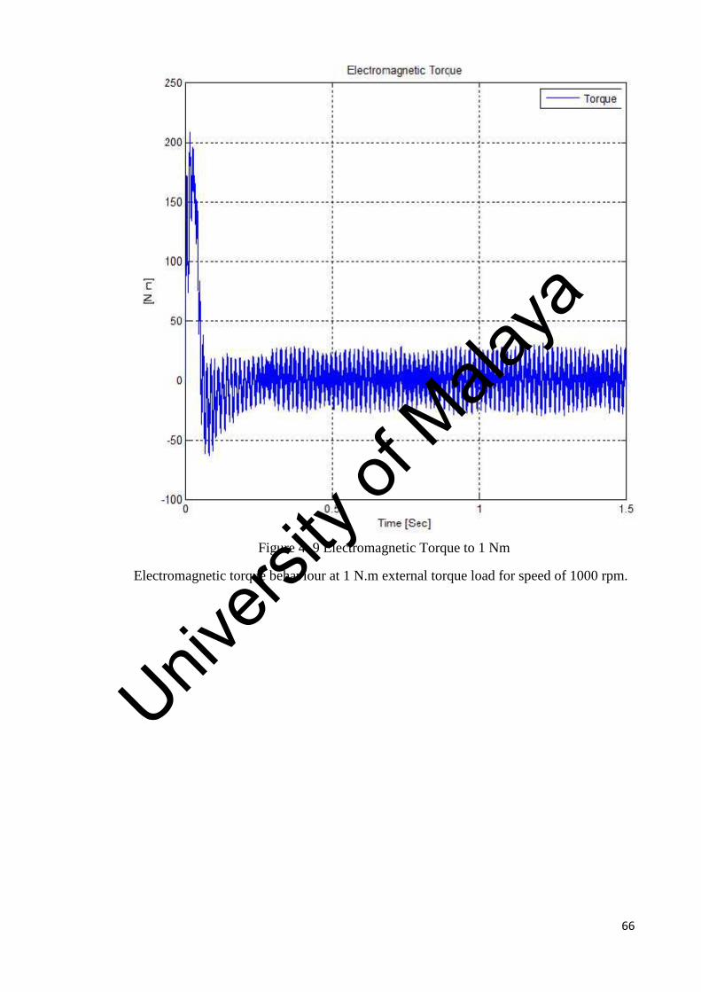
66
Figure 4. 9 Electromagnetic Torque to 1 Nm
Electromagnetic torque behaviour at 1 N.m external torque load for speed of 1000 rpm.
Univers
ity of
Mala
ya
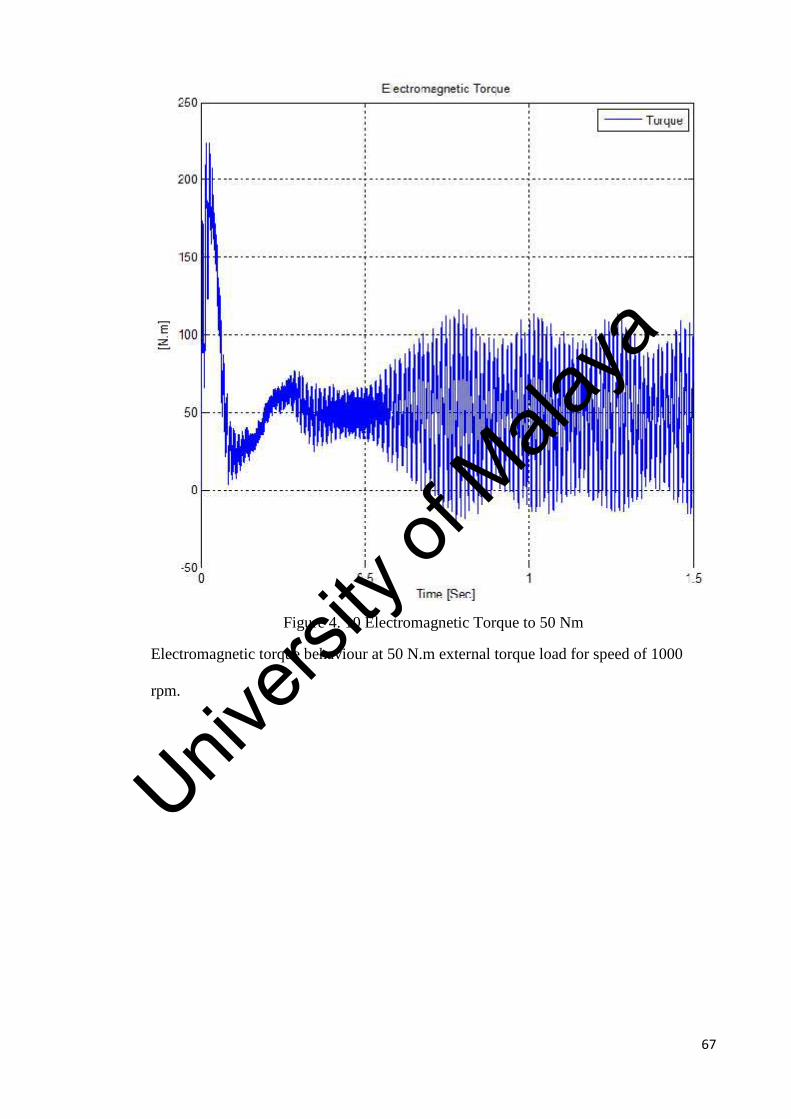
67
Figure 4. 10 Electromagnetic Torque to 50 Nm
Electromagnetic torque behaviour at 50 N.m external torque load for speed of 1000
rpm.
Univers
ity of
Mala
ya

68
4.1 Discussion of results
Adaptive observer scheme is tested on different values of external load torque, and the
reference speeds. From tested results in Matlab simulink, it gives the best result of
Electromagnetic torque on the value of external load torque 50Nm with the reference
speed of 490rpm which is constant at very low transient. Higher speed up to 1000rpm is
also tested on which external load 1 Nm gives also good result of speed which is stable
also at very low transient time.
System is configured at the speed starts from 490 [rpm] to [1000rpm] with external load
form 1 [Nm] to 50 [Nm]. Results as per required speed can achieved at required external
torque; for that there is need of change in variations parameter of induction motor,
adaptive flux until the system becomes stable. For adaptive observer it is confirmed
from the results that for getting the value which is required are depending on the
accurate parameters variations. As speed 490rpm is stable on external load 50 N.m, 0.96
flux value; any variation in other parameters of induction motor will make the system
disable. Any required speed with respect to external load using adaptive observer can be
attained by adjusting the parameter of induction motor until the system becomes stable.
Univers
ity of
Mala
ya
69
CHAPTER FIVE: CONCLUSION AND RECOMENDATION
5.1 Conclusion
The design and analysis of adaptive observer for controlling the performance of
induction motor has been presented. Different types of sensorless techniques were
discussed and reviewed together with the adaptive observer technique. The objective of
reviewing all techniques was to arrange the speed sensorless method techniques along
with the importance of merits and demerits for each method. The comparison between
different estimation of speed methods based on devised set of criteria was also
introduced. Mostly the exchanges which occur are between the simplicity regarding
implementation and the behaviour of over all system. Nevertheless, for the justification
of the certain scheme regarding specific applications from the results of each method is
considered a useful tool and all techniques are considered yet as powerful according to
the needs of specific requirements for the system.
For low speed procedure there is a need of introducing low speed application technique
such as; the technique of frequency signal injection method and rotor slot harmonic
methods, system which have high noise; mostly Extended Kalman Filter (EKF) is
preferable, due to noise reason EKF is designed as like in which can perform most
desirable filtration. Slide Mode Observer (SMO) gives better speed estimation although
it is required to remove the chattering problems from the system. Artificial Intelligence
technique has the problem of complexity and the large time in computation although it
also demonstrates the better results.
Adaptive flux observer technique is presented in new way, as improved technique for
the induction motor, based on the correction of the value of the stator resistance and the
estimation of the load torque. The estimation of the torque is based on the use of the
error between real and estimated speed of induction motor, this will have to improve the
performances of the adaptive flux observer. The results show that the proposed adaptive
Univers
ity of
Mala
ya

70
observer offers better performances while tracking the speed and the flux, even in
presence of stator resistance variation.
5.2 Recommendation
As there are advantages and disadvantages of sensorless techniques, due to that all
techniques are important for specific application purpose; none of them would be
discarded for any disadvantage reason, all are useful. For example as Artificial
Intelligence (AI) system has better results but has problem of computation time and
complexity. However, AI techniques using with adaptive observer criteria can make
system more stable. It is highly recommended idea which comes after review of all
sensorless technique that by using the advantages of all sensorless techniques according
to needs such as; variation to parameters , configure system according to requirement ,
reduce complexity and try to reduce disadvantages for making the system more reliable
and accurate. Such adaptive observer scheme is preferred and possible by using
combination of techniques, SMO technique together with AI can give better results just
by eliminating chattering problem from SMO and reduce the complexity and
computation time of AI system together with variation in parameters.
Univers
ity of
Mala
ya
71
REFERENCES
Abdalla, T. Y., et al. (2010). Direct torque control system for a three phase inductionmotor with fuzzy logic based speed Controller. Energy, Power and Control (EPC-IQ),2010 1st International Conference on.
Abu-Rub, H. and J. Guzinski (2011). Simple observer for induction motor speedsensorless control. IECON 2011 - 37th Annual Conference on IEEE IndustrialElectronics Society.
Al-Tayie, J. K. and P. P. Acarnley (1997). "Estimation of speed, stator temperature androtor temperature in cage induction motor drive using the extended Kalman filteralgorithm." Electric Power Applications, IEE Proceedings - 144(5): 301-309.
Alamir, M. (2002). "Sensitivity analysis in simultaneous state/parameter estimation forinduction motors." Int. J. of Control 75(n°10): pp.753-758.
Campbell, J. and M. Sumner (2002). "Practical sensorless induction motor driveemploying an artificial neural network for online parameter adaptation." Electric PowerApplications, IEE Proceedings - 149(4): 255-260.
Consoli, A., et al. (2004). "Slip-frequency detection for indirect field-oriented controldrives." Industry Applications, IEEE Transactions on 40(1): 194-201.
Consoli, A., et al. (2004). "Speed- and current-sensorless field-oriented induction motordrive operating at low stator frequencies." Industry Applications, IEEE Transactions on40(1): 186-193.
da Silva, E. R. and M. D. Kankam (1997). Speed sensorless induction motor drives forelectrical actuators: schemes, trends and tradeoffs. Aerospace and ElectronicsConference, 1997. NAECON 1997., Proceedings of the IEEE 1997 National.
Derdiyok, A. (2005). "Speed-Sensorless Control of Induction Motor Using aContinuous Control Approach of Sliding-Mode and Flux Observer." IndustrialElectronics, IEEE Transactions on 52(4): 1170-1176.
Dr.JBV Subrahmanyam, T. S., TC Subramanyam,PK Sahoo,P Sankar (2011)."APPLICATION OF VECTOR CONTROL TECHNIQUE TO AC MOTORS." IJAERVol. No. 2(Issue No. V).
Edelbaher, G., et al. (2006). "Low-speed sensorless control of induction Machine."Industrial Electronics, IEEE Transactions on 53(1): 120-129.
Elloumi, M., et al. (1998). Survey of speed sensorless controls for IM drives. IndustrialElectronics Society, 1998. IECON '98. Proceedings of the 24th Annual Conference ofthe IEEE.
Univers
ity of
Mala
ya
72
Garcia Soto, G., et al. (1999). "Reduced-order observers for rotor flux, rotor resistanceand speed estimation for vector controlled induction motor drives using the extendedKalman filter technique." Electric Power Applications, IEE Proceedings - 146(3): 282-288.
Hinkkanen, M., et al. (2005). "Flux observer enhanced with low-frequency signalinjection allowing sensorless zero-frequency operation of induction motors." IndustryApplications, IEEE Transactions on 41(1): 52-59.
Holtz, J. (2002). "Sensorless control of induction motor drives." Proceedings of theIEEE 90(8): 1359-1394.
Holtz, J. (2006). "Sensorless Control of Induction Machines—With or WithoutSignal Injection?" Industrial Electronics, IEEE Transactions on 53(1): 7-30.
Holtz, J. and Q. Juntao (2002). "Sensorless vector control of induction motors at verylow speed using a nonlinear inverter model and parameter identification." IndustryApplications, IEEE Transactions on 38(4): 1087-1095.
Holtz, J. and Q. Juntao (2003). "Drift- and parameter-compensated flux estimator forpersistent zero-stator-frequency operation of sensorless-controlled induction motors."Industry Applications, IEEE Transactions on 39(4): 1052-1060.
Hossein Madadi Kojabadia, a. L. C. (2005). "Comparative study of pole placementmethods in adaptive flux observers." Control Engineering Practice Elsevier, 13: pp.749–757.
Huang, M. S. and C. M. Liaw (2003). "Improved field-weakening control for IFOinduction motor." Aerospace and Electronic Systems, IEEE Transactions on 39(2): 647-659.
Ilas, C., et al. (1994). Comparison of different schemes without shaft sensors for fieldoriented control drives. Industrial Electronics, Control and Instrumentation, 1994.IECON '94., 20th International Conference on.
J.P. Caron, J. P. H. (1995). "Modeling and Control of Induction Machine. TechnipEdition."
Jingchuan, L., et al. (2005). "An adaptive sliding-mode observer for induction motorsensorless speed control." Industry Applications, IEEE Transactions on 41(4): 1039-1046.
Jun, R., et al. (2012). Modeling and simulation of vector control system forasynchronous motor. Electronic System-Integration Technology Conference (ESTC),2012 4th.
Univers
ity of
Mala
ya
73
Khalil, H. K., et al. (2009). "Speed Observer and Reduced Nonlinear Model forSensorless Control of Induction Motors." Control Systems Technology, IEEETransactions on 17(2): 327-339.
Khan, M. R. and A. Iqbal (2012). Model reference adaptive system with simplesensorless flux observer for induction motor drive: MRAS with simple sensorless fluxobserver for induction motor drive. Power Electronics, Drives and Energy Systems(PEDES), 2012 IEEE International Conference on.
Khater, M. M., et al. (2006). A comparative study of sliding mode and Model ReferenceAdaptive Speed observers for induction motor drives. Power Systems Conference,2006. MEPCON 2006. Eleventh International Middle East.
kojabadi, M. (2005). "Simulation and experimental studies of model reference adaptivesystem for sensorless induction motor drive." Simulation Modeling practice and theory,Elsevier: pp. 451–464.
Korlinchak, C. and M. Comanescu (2012). "Sensorless field orientation of an inductionmotor drive using a time-varying observer." Electric Power Applications, IET 6(6): 353-361.
Lascu, C. and G. Andreescu (2006). "Sliding-mode observer and improved integratorwith DC-offset compensation for flux estimation in sensorless-controlled inductionmotors." Industrial Electronics, IEEE Transactions on 53(3): 785-794.
Lesan, A. Y. E., et al. (2012). Comparative study of speed estimation techniques forsensorless vector control of induction machine. IECON 2012 - 38th Annual Conferenceon IEEE Industrial Electronics Society.
Levi, E. and W. Mingyu (2002). "A speed estimator for high performance sensorlesscontrol of induction motors in the field weakening region." Power Electronics, IEEETransactions on 17(3): 365-378.
Levi, E. and W. Mingyu (2003). "Online identification of the mutual inductance forvector controlled induction motor drives." Energy Conversion, IEEE Transactions on18(2): 299-305.
Liu, J. and X. Wang (2008). Adaptive stator and rotor resistance identification forinduction machine without rotational transducer. Control Conference, 2008. CCC 2008.27th Chinese.
Lopez, J. C., et al. (2006). "Novel Fuzzy Adaptive Sensorless Induction Motor Drive."Industrial Electronics, IEEE Transactions on 53(4): 1170-1178.
Univers
ity of
Mala
ya
74
M. Alexandru , R. B., G. Ghelardi, S.M.Tenconi (2002). "An AC motor closed loopperformances with different rotor flux observers.MCFA Annals, Vol III, pp.1-3.".
M.S. ZAKY, M. K., H. YASIN and S.S. SHOKRALLA (2008). "Speed-SensorlessControl of Induction Motor Drives (Review Paper)." Volume 49.
Marwali, M. N. and A. Keyhani (1997). A comparative study of rotor flux based MRASand back EMF based MRAS speed estimators for speed sensorless vector control ofinduction machines. Industry Applications Conference, 1997. Thirty-Second IASAnnual Meeting, IAS '97., Conference Record of the 1997 IEEE.
Myoung-Ho, S. and H. Dong-Seok (2003). "Speed sensorless stator flux-orientedcontrol of induction machine in the field weakening region." Power Electronics, IEEETransactions on 18(2): 580-586.
Qilian, L. and J. M. Mendel (2000). "Interval type-2 fuzzy logic systems: theory anddesign." Fuzzy Systems, IEEE Transactions on 8(5): 535-550.
Rafiq, M. A., et al. (2012). Artificial Neural Network based speed tracking of a fieldoriented induction motor drive. Electrical & Computer Engineering (ICECE), 2012 7thInternational Conference on.
Rahman, M. F., et al. (2003). "A direct torque-controlled interior permanent-magnetsynchronous motor drive without a speed sensor." Energy Conversion, IEEETransactions on 18(1): 17-22.
Rashed, M. and A. F. Stronach (2004). "A stable back-EMF MRAS-based sensorlesslow-speed induction motor drive insensitive to stator resistance variation." ElectricPower Applications, IEE Proceedings - 151(6): 685-693.
Ravi Teja, A. V., et al. (2012). "A New Model Reference Adaptive Controller for FourQuadrant Vector Controlled Induction Motor Drives." Industrial Electronics, IEEETransactions on 59(10): 3757-3767.
Sangsefidi, Y., et al. (2012). A simple and low-cost method for three-phase inductionmotor control in high-speed applications. Power Electronics and Drive SystemsTechnology (PEDSTC), 2012 3rd.
Savoia, A., et al. (2012). Adaptive flux observer for induction machines with on-lineestimation of stator and rotor resistances. Power Electronics and Motion ControlConference (EPE/PEMC), 2012 15th International.
Schauder, C. (1992). "Adaptive speed identification for vector control of inductionmotors without rotational transducers." Industry Applications, IEEE Transactions on28(5): 1054-1061.
Univers
ity of
Mala
ya
75
Sedhuraman, K., et al. (2012). Comparison of learning algorithms for neural networkbased speed estimator in sensorless induction motor drives. Advances in Engineering,Science and Management (ICAESM), 2012 International Conference on.
Seong-Hwan, K., et al. (2001). "Speed-sensorless vector control of an induction motorusing neural network speed estimation." Industrial Electronics, IEEE Transactions on48(3): 609-614.
Sheng-Ming, Y. and K. Shuenn-Jenn (2000). "Performance evaluation of a velocityobserver for accurate velocity estimation of servo motor drives." Industry Applications,IEEE Transactions on 36(1): 98-104.
Siddique, A., et al. (2003). Applications of artificial intelligence techniques forinduction machine stator fault diagnostics: review. Diagnostics for Electric Machines,Power Electronics and Drives, 2003. SDEMPED 2003. 4th IEEE InternationalSymposium on.
Smidl, V. and Z. Peroutka (2012). "Advantages of Square-Root Extended Kalman Filterfor Sensorless Control of AC Drives." Industrial Electronics, IEEE Transactions on59(11): 4189-4196.
Staines, C. S., et al. (2006). "Sensorless control of induction Machines at zero and lowfrequency using zero sequence currents." Industrial Electronics, IEEE Transactions on53(1): 195-206.
Sun, K. and Y. Zhao (2010). A speed observer for speed sensorless control of inductionmotor. Future Computer and Communication (ICFCC), 2010 2nd InternationalConference on.
Tae-Sung, K., et al. (2005). "Speed sensorless stator flux-oriented control of inductionmotor in the field weakening region using Luenberger observer." Power Electronics,IEEE Transactions on 20(4): 864-869.
Tajima, H., et al. (2000). Consideration about problems and solutions of speedestimation method and parameter tuning for speed sensorless vector control of inductionmotor drives. Industry Applications Conference, 2000. Conference Record of the 2000IEEE.
Tajjudin, M., et al. (2012). Simple PID tuning using relay perturbation with errorswitching. System Engineering and Technology (ICSET), 2012 InternationalConference on.
Tarek BENMILOUD, A. O. (2011). "Improved Adaptive Flux Observer of an InductionMotor with Stator Resistance Adaptation." PRZEGLĄD ELEKTROTECHNICZNY(Electrical Review), ISSN 0033-2097, R. 87 NR 9a/2011.
Univers
ity of
Mala
ya
76
Ugale, R. T., et al. (2012). A low cost fast data acquisition system for capturing electricmotor starting and dynamic load transients. Power Electronics, Drives and EnergySystems (PEDES), 2012 IEEE International Conference on.
Vasic, V., et al. (2003). "A stator resistance estimation scheme for speed sensorlessrotor flux oriented induction motor drives." Energy Conversion, IEEE Transactions on18(4): 476-483.
Venkataramana Naik, N. and S. P. Singh (2012). A novel type-2 fuzzy logic control ofinduction motor drive using Scalar Control. Power Electronics (IICPE), 2012 IEEE 5thIndia International Conference on.
Volat, M. A. O. a. C. (2000). "Simulation of a Direct Field-Oriented Controller for anInduction Motor Using Matlab/Simulink. Proceeding of the IASTED InternationalConference Modelling and Simulation - Pittsburgh, Pennsylvania, USA."
Wang, P., et al. (2010). Speed-sensorless direct torque control system of inductionmotor. Control and Decision Conference (CCDC), 2010 Chinese.
Wolbank, T. M., et al. (2000). Comparison of different winding schemes reference totheir application on speed sensorless control of induction machines. IndustrialElectronics Society, 2000. IECON 2000. 26th Annual Confjerence of the IEEE.
Zaky, M. S. (2012). "Stability Analysis of Speed and Stator Resistance Estimators forSensorless Induction Motor Drives." Industrial Electronics, IEEE Transactions on 59(2):858-870.
Zamora, J. L. and A. Garcia-Cerrada (2000). "Online estimation of the stator parametersin an induction motor using only voltage and current measurements." IndustryApplications, IEEE Transactions on 36(3): 805-816.
Univers
ity of
Mala
ya
Recommended