Embed Size (px)
Citation preview

Consistency without Inference Instrumental Variables in Practical Application
Alwyn Young
London School of Economics This draft June 2018
Abstract
I use Monte Carlo simulations the jackknife and multiple forms of the bootstrap to study
a comprehensive sample of 1359 instrumental variables regressions in 31 papers published in the
journals of the American Economic Association Monte Carlo simulations based upon published
regressions show that non-iid error processes adversely affect the size and power of IV estimates
while increasing the bias of IV relative to OLS producing a very low ratio of power to size and
mean squared error that is almost always larger than biased OLS Weak instrument pre-tests
based upon F-statistics are found to be largely uninformative of both size and bias In published
papers statistically significant IV results generally depend upon only one or two observations or
clusters excluded instruments often appear to be irrelevant there is little statistical evidence that
OLS is actually substantively biased and IV confidence intervals almost always include OLS
point estimates
I am grateful to David Broadstone Brian Finley and anonymous referees for valuable suggestions and to
Ruoqi Zhou for excellent research assistance
2
I Introduction
The economics profession is in the midst of a ldquocredibility revolutionrdquo (Angrist and
Pischke 2010) in which careful research design has become firmly established as a necessary
characteristic of applied work A key element in this revolution has been the use of instruments
to identify causal effects free of the potential biases carried by endogenous ordinary least squares
regressors The growing emphasis on research design has not gone hand in hand however with
equal demands on the quality of inference Despite the widespread use of Eicker (1963)-Hinkley
(1977)-White (1980) robust and clustered covariance estimates the implications of non-iid error
processes for the quality of inference and their interaction in this regard with regression and
research design has not received the attention it deserves Heteroskedastic and correlated errors
produce test statistics whose dispersion is typically much greater than believed particularly in
highly leveraged regressions which is the dominant feature of regression design in published
papers This adversely affects inference in both ordinary least squares (OLS) and two stage least
squares (hereafter 2SLS or IV) but more so in the latter where confidence in results depends
upon an assessment of the strength of both first and second stage relations
In this paper I use Monte Carlos the jackknife and multiple forms of the bootstrap to
study the distribution of coefficients and test statistics in a comprehensive sample of 1359 2SLS
regressions in 31 papers published in the journals of the American Economic Association
Subject to some basic rules regarding data and code availability and methods applied I have not
allowed myself any discretion in picking papers or regressions and use all papers produced by a
keyword search on the AEA website I maintain throughout the exact specification used by
authors and their identifying assumption that the excluded instruments are orthogonal to the
second stage residuals When bootstrapping jackknifing or generating artificial residuals for
Monte Carlos I draw samples in a fashion consistent with the error dependence within groups of
observations and independence across observations implied by authorsrsquo standard error
calculations Thus this paper is not about point estimates or the validity of fundamental
3
assumptions but rather concerns itself with the quality of inference within the framework laid
down by authors themselves
Monte Carlos using the regression design found in my sample and artificial error
disturbances with a covariance structure matching that observed in 1st and 2nd stage residuals
show how non-iid errors damage the relative quality of inference using 2SLS Non-iid errors
weaken 1st stage relations raising the relative bias of 2SLS and generating mean squared error
that is larger than biased OLS in almost all published papers Non-iid errors also increase the
probability of spuriously large test statistics when the instruments are irrelevant particularly in
highly leveraged regressions and particularly in joint tests of coefficients ie 1st stage F tests
Consequently while 1st stage relations weaken 1st stage pre-tests become uninformative
providing little or no protection against 2SLS size distortions or bias 2SLS standard error
estimates based upon the assumption of a non-stochastic 1st stage relationship become more
volatile and tail values of the t-statistic are dominated by unusually low realizations of the
standard error rather than unexpected deviations of mean effects from the null In the top third
most highly leveraged papers in my sample the ratio of power to size approaches one ie 2SLS
is scarcely able to distinguish between a null of zero and the alternative of the mean effects
found in published tables
Monte Carlos show however that the jackknife and (particularly) the bootstrap allow for
2SLS and OLS inference with accurate size and a much higher ratio of power to size than
achieved using clusteredrobust covariance estimates Thus while the bootstrap does not undo
the increased bias of 2SLS brought on by non-iid errors it nevertheless allows for improved
inference under these circumstances Inference using conventional standard errors in 2SLS is
based on an estimate of a moment that often does not exist (as the coefficient has no finite
variance when exactly identified) under the assumption of an immutable 1st stage relationship
that is clearly invalid (as point estimates in highly leveraged regressions depend heavily upon the
realizations of just one or two residuals) Not surprisingly the bootstraprsquos use of resampling to
estimate the percentiles of distributions which always exist does much better While asymptotic
4
theory favours the resampling of the t-statistic I find that avoiding the finite sample 2SLS
standard estimate altogether and focusing on the bootstrap resampling of the coefficient
distribution alone provides the best performance with tail rejection probabilities on IV
coefficients that are very close to nominal size in iid non-iid low and high leverage settings
When published results are examined through the lens of the jackknife and bootstrap a
number of weaknesses are revealed In published papers about frac12 to ⅔ of 01 significant IV
results depend upon only one or two outlier observations or clusters and rest upon a finding of
unusually small standard errors rather than surprising (under the null) mean effects First stage
relations when re-examined through the jackknife or bootstrap cannot reject the null that the
excluded instruments are irrelevant in about frac14 to ⅓ of cases while jackknifed and bootstrapped
Durbin (1954) - Wu (1973) - Hausman (1978) tests find little evidence that OLS is substantively
biased despite large proportional and frequent sign differences between OLS and 2SLS point
estimates as 2SLS estimation is found to be so inaccurate that 2SLS confidence intervals almost
always include OLS point estimates In sum whatever the biases of OLS may be in practical
application with non-iid error processes and highly leveraged regression design the performance
of 2SLS methods deteriorates so much that it is rarely able to identify parameters of interest
more accurately or substantively differently than is achieved by OLS The third of my sample
with the lowest maximum observational leverage does better on all metrics but even here only frac12
of papers provide any regressions with results that are significantly distinguishable from OLS
The concern with the quality of inference in 2SLS raised in this paper is not new
Sargan in his seminal 1958 paper raised the issue of efficiency and the possibility of choosing
the biased but more accurate OLS estimator leading later scholars to explore relative efficiency
in Monte Carlo settings (eg Summers 1965 Feldstein 1974) The current professional emphasis
on first stage F-statistics as pre-tests originates in Nelson and Startz (1990a b) who used
examples to show that size distortions can be substantial when the strength of the first stage
relationship is weak and Bound Jaeger and Baker (1995) who emphasized problems of bias and
inconsistency with weak instruments These papers spurred path-breaking research such as
5
Staiger and Stock (1997) and Stock and Yogorsquos (2005) elegant derivation and analysis of weak
instrument asymptotic distributions renewed interest (eg Dufour 2003 Baum Schaffer and
Stillman 2007 Chernozhukov and Hansen 2008) in older weak instrument robust methods such
as that of Anderson-Rubin (1949) and motivated the use of such techniques in critiques of
selected papers (eg Albouy 2012 Bazzi and Clemens 2013) The theoretical and Monte Carlo
work that motivates this literature is largely iid based a notable exception being Olea amp Pflueger
(2013) who argue that heteroskedastic error processes weaken 1st stage relations and based
upon asymptotic approximations propose a bias test closely related to the 1st stage clustered
robust F-statistic This paper supports Olea amp Pfluegerrsquos insight that non-iid errors effectively
weaken 1st stage relations brings to the fore earlier concerns regarding the practical relative
efficiency of 2SLS shows that iid-motivated weak instrument pre-tests and weak instrument
robust methods perform poorly when misapplied in non-iid settings and highlights the errors
induced by finite sample inference using asymptotically valid clusteredrobust covariance
estimates in highly leveraged settings including even the Olea amp Pflueger bias test
The paper proceeds as follows After a brief review of notation in Section II Section III
describes the rules used to select the sample and its defining characteristics highlighting the
presence of non-iid errors high leverage and sensitivity to outliers Section IV presents Monte
Carlos patterned on the regression design and error covariance found in my sample showing
how non-iid errors worsen inference of all sorts but especially degrade the ratio of power to size
in IV tests while raising the relative bias of 2SLS estimation 1st stage pre-tests are found to be
largely uninformative although the Olea amp Pflueger bias test effectively separates low and high
bias in low leverage over-identified 2SLS regressions Section V provides a thumbnail review of
jackknife and ldquopairsrdquo and ldquowildrdquo bootstrap methods The pairs resampling of the coefficient
distribution is found to provide a low cost means of performing multiple 1st and 2nd stage tests
with tail rejection probabilities as accurate as other methods and very close to nominal size in
tests of IV coefficients in particular Section VI re-examines the 2SLS regressions in my sample
using all of the jackknife and bootstrap methods finding the results mentioned above while
6
Section VII concludes An on-line appendix provides alternative versions of many tables further
comparison of the accuracy of different bootstrap methods and Monte Carlos of some popular
weak instrument robust methods showing that these which do not directly address the issue of
non-iid errors are not panaceas and in some cases perform much worse than 2SLS
All of the results of this research are anonymized Thus no information can be provided
in the paper public use files or private conversation regarding results for particular papers
Methodological issues matter more than individual results and studies of this sort rely upon the
openness and cooperation of current and future authors For the sake of transparency I provide
complete code (in preparation) that shows how each paper was analysed but the reader eager to
know how a particular paper fared will have to execute this code themselves
II Notation and Formulae
It is useful to begin with some notation and basic formulae to facilitate the discussion
which follows With bold lowercase letters indicating vectors and uppercase letters matrices the
data generating process is taken as given by
)1( vγXπZYuδXYy
where y is the n x 1 vector of second stage outcomes Y the n x 1 matrix of endogenous
regressors X the n x kX matrix of included exogenous regressors Z the n x kZ matrix of
excluded exogenous regressors (instruments) and u and v the n x 1 vectors of second and first
stage disturbances The remaining (Greek) letters are parameters with β representing the
parameter of interest Although in principal there might be more than one endogenous right-
hand side variable ie Y is generally n x kY in practical work this is exceedingly rare (see
below) and this paper focuses on the common case where kY equals 1
The nuisance variables X and their associated parameters are of no substantive interest
so I use ~ to denote the residuals from the projection on X and characterize everything in terms of
these residuals For example with ^ denoting estimated and predicted values the coefficient
estimates for OLS and 2SLS are given by
7
YZ)ZZ(ZYyYYYyYYY 1 ~~~~~~ where~~
)~~
(ˆ~~)
~~(ˆ)2( 1
21
slsols
Finally although the formulae are well known to avoid any confusion it is worth spelling out
that in referring to ldquodefaultrdquo covariance estimates below I mean
ˆ~~
)ˆV( ampˆ)~~
()ˆ(ˆ)~~
()ˆ()3( 2212
21vuslsuols VV 1)ZZ(πYYYY
where 2ˆu and 2ˆv equal the sum of the (OLS or 2SLS) squared residuals divided by n minus the
k right hand side variables while in the case of ldquoclusteredrobustrdquo covariance estimates I mean
11
222
)~~
(~
ˆˆ~
)~~
()ˆ( amp)
~~(
~ˆˆ
~
)ˆ()
~~(
~ˆˆ
~
)ˆ()4(
ZZZvvZZZπ
YY
YuuY
YY
YuuY
iiiIi
i
iiiIi
iiiiIi
i
cV
c
V
c
V slsols
where i denotes the group of clustered observations (or individual observations when merely
robust) I the set of all such groupings u and v the second and first stage residuals c a finite
sample adjustment (eg n(n-k) in the robust case) and where I have made use of the fact that the
inner-product of Y is a scalar
Equations (2) and (3) highlight the issues that have arisen in the evaluation of 2SLS over
the years The older concern regarding the potential inefficiency of 2SLS relative to OLS (eg
Sargan 1958 Summers 1965 Feldstein 1974) stems from the fact that 2SLS gives up some of the
variation of the right hand side variable using the predicted values of Y~
to estimate β2sls as
compared to the full variation of the actual values of Y~
used in the calculation of βols The more
recent emphasis on the strength of 1st stage relations (eg Nelson amp Startz 1990a Bound Jaeger
amp Baker 1995 and Stock amp Yogo 2005) finds its expression in two places First when the 1st
stage relation is weak the predicted values of Y~
are more heavily influenced by the finite sample
correlation of the excluded instruments with the 1st stage disturbances producing β2sls estimates
that are biased in the direction of OLS Second in the 2sls covariance estimate the predicted
values of Y~
are taken as fixed and consequently independent of the 2nd stage residuals1 This
1The issue is not so much fixity as the implicit assumption that they are independent of the 2nd stage
disturbances Consider the ideal case of unbiased OLS estimates with iid normal disturbances The default covariance estimate calculates the distribution of coefficients across the realizations of the residuals for fixed regressors As inference in this case is exact conditional on the regressors it is also exact unconditionally across all realizations of the regressors when these are stochastic In the case of 2SLS in finite samples this thought
8
requires that the first stage relationship be strong enough so as to make the predicted values
virtually non-stochastic and only minimally dependent upon the realization of the correlated 1st
stage disturbances
A well-known re-expression of the 2SLS coefficient estimates provides a different
perspective on these issues Allowing ab to denote the OLS coefficient found in projecting
variable a on b we have
1 k when ˆ
ˆor
ˆ~~ˆ
ˆ~~ˆˆˆˆ)5( Z
~~
~~
~~~~
~~~~
2~~
ZY
Zy
ZYZY
ZyZY
Yy β)ZZ(β
β)ZZ(β
slsols
The 2SLS coefficient estimate is the ratio (or weighted ratio in the over-identified case) of two
OLS coefficients the reduced form Zy~~ divided by the 1st stage ZY
~~ Estimating something
using the ratio of two projections is less efficient than estimating it directly if that is possible
The 2SLS covariance estimates in (3) and (4) look like the estimated variance of a stochastic
Zy~~ multiplied by the constant 1 ZY
~~ 2 Thus the 2SLS variance estimate treats the 1st stage
component of the 2SLS coefficient estimate as fixed
III The Sample
My sample is based upon a search on wwwaeaweborg using the keyword instrument
covering the American Economic Review and the American Economic Journals for Applied
Economics Economic Policy Microeconomics and Macroeconomics which at the time of its
implementation yielded papers up through the July 2016 issue of the AER I then dropped
papers that
(a) did not provide public use data files and Stata do-file code (b) did not include instrumental variables regressions (c) used non-linear methods or non-standard covariance estimates (d) provided incomplete data or non-reproducible regressions
Public use data files are necessary to perform any analysis and I had prior experience with Stata experiment is not valid because the predicted first stage estimates depend upon 1st stage residuals which are correlated with the 2nd stage disturbances
2Except that the estimated σ2 is the estimated variance of u whereas for the reduced form βyZ the relevant variance is that of βv + u
9
and hence could analyse do-files for this programme at relatively low cost Stata is by far the
most popular programme as among papers that provide data only five make use of other
software The keyword search brought up a number of papers that deal with instruments of
policy rather than instrumental variables and these were naturally dropped from the sample
Conventional linear two stage least squares with either the default or clusteredrobust
covariance estimate is the overwhelmingly dominant approach so to keep the discussion
focused I dropped four rare deviations These include two papers that used non-linear IV
methods one paper which clustered on two variables the union of which encompassed the entire
sample making it impossible to implement a bootstrap that respects the cross-correlations the
authors believe exist in the data and another paper which uniquely used auto-correlation
consistent standard errors (in only 6 regressions) using a user-written routine that does not
provide formulas or references in its documentation One paper used Fullerrsquos modification of
limited information maximum likelihood (LIML) methods Since this method is considered a
weak instrument robust alternative to 2SLS I keep the paper in the sample examining its
regressions with conventional 2SLS (LIML and Fuller methods are studied in the on-line
appendix) A smattering of GMM methods appear in two papers whose 2SLS regressions are
otherwise included in the sample Inference in the generalized method of moments raises issues
of its own that are best dealt with elsewhere so I exclude these regressions from the analysis
Many papers provide partial data indicating that users should apply to third parties for
confidential data necessary to reproduce the analysis As the potential delay and likelihood of
success in such applications is indeterminate I dropped these papers from my sample One
paper provided completely ldquobrokenrdquo code with key variables missing from the data file and was
dropped from the sample Outside of this case however code in this literature is remarkably
accurate and with the exception of two regressions in one paper (which were dropped)3 I was
able to reproduce within rounding error or miniscule deviations on some coefficients all of the
3I also dropped 2 other regressions that had 10 million observations as a jackknife bootstrap and Monte
Carlo analysis of these regressions is beyond the computational resources available to me
10
regressions reported in tables I took as my sample only IV regressions that appear in tables
Alternative specifications are sometimes discussed in surrounding text but catching all such
references and linking them to the correct code is extremely difficult By limiting myself to
specifications presented in tables I was able to use coefficients standard errors and
supplementary information like sample sizes and test statistics to identify interpret and verify the
relevant parts of authorsrsquo code Cleaning of the sample based upon the criteria described above
produced 1400 2SLS regressions in 32 papers Only 41 of these however contain more than
one endogenous right hand side variable As 41 observations are insufficient to draw meaningful
conclusions I further restricted the analysis to regressions with only one endogenous variable
As shown in Table I below the final sample consists of 31 papers 16 appearing in the
American Economic Review and 15 in other AEA journals Of the 1359 IV regressions in these
papers 1087 are exactly identified by one excluded instrument and 272 are overidentified
When equations are overidentified the number of instruments can be quite large with an average
of 17 excluded instruments (median of 5) in 13 papers Thus econometric issues concerning the
higher dimensionality of instruments are relevant in a substantial subset of equations and papers
Although instrumental variables regressions are central to the argument in all of these papers
with the keyword ldquoinstrumentrdquo appearing in either the abstract or the title the actual number of
IV regressions varies greatly with 5 papers presenting 98 to 286 such regressions while 9 have
only between 2 to 10 In consideration of this and the fact there is a great deal of similarity
within papers in regression design in presenting averages in tables and text below unless
otherwise noted I always take the average across papers of the within paper average Thus each
paper carries an equal weight in determining summary results
Turning to statistical inference all but one of the papers in my sample use the Eicker
(1963)-Hinkley (1977)-White (1980) robust covariance matrix or its multi-observation cluster
extension Different Stata commands make use of different distributions to evaluate the
significance of the same 2SLS estimating equation with the sample divided roughly equally
between results evaluated using the t and F (with finite sample covariance corrections) and those
11
Table I Characteristics of the Sample
31 papers 1359 2SLS regressions
journal of 2SLS regressions
excluded instruments
covariance estimate
distribution
16 6 4 5
AER AEJ A Econ AEJ E Policy AEJ Macro
9 9 8 5
2-10 11-26 35-72 98-286
1087 138 134
1 2-5 6-60
105 1039
215
default clustered robust
753 606
t amp F N amp chi2
Notes AER = American Economic Review AEJ = American Economic Journal Applied Economics Economic Policy and Macro t F N amp chi2 = t F standard normal and chi-squared distributions
evaluated using the normal and chi2 In directly evaluating authorsrsquo results I use the
distributions and methods they chose For more general comparisons however I move
everything to a consistent basis using clusteredrobust4 covariance estimates and the t and F
distributions for all 2SLS and OLS results
Table II shows that non-normality intra-cluster correlation and heteroskedasticity of the
disturbances are important features of the data generating process in my sample Using Statarsquos
test of normality based upon skewness and kurtosis I find that in the average paper more than
80 of the OLS regressions which make up the 2SLS point estimates reject the null that the
residuals are normal In equations which cluster cluster fixed effects are also found to be
significant more than 80 of the time In close to frac12 of these regressions the authorsrsquo original
specification includes cluster fixed effects but where there is smoke there is likely to be fire ie
it is unlikely that the cluster correlation of residuals is limited to a simple mean effect a view
apparently shared by the authors as they cluster standard errors despite including cluster fixed
effects Tests of homoskedasticity involving the regression of squared residuals on the authorsrsquo
right-hand side variables and cluster fixed effects (where authors cluster) using the test statistics
and distributions suggested by Koenker (1981) and Wooldridge (2013) reject the null between ⅔
and 80 of the time In Monte Carlos further below I find that while non-normality is of
4I use the robust covariance estimate for the one paper that used the default covariance estimate throughout
and also cluster four regressions that were left unclustered in papers that otherwise clustered all other regressions
12
Table II Tests of Normality Cluster Correlation and Heteroskedasticity (average across 31 papers of fraction of regressions rejecting the null)
Y on Z X (1st stage)
y on Z X (reduced form)
y on Y X (OLS)
01 05 01 05 01 05
normally distributed residuals 807 831 811 882 830 882
no cluster fixed effects 846 885 855 899 835 879
homoscedastic (K) on Z X or Y X 739 806 635 698 657 727
homoskedastic (W) on Z X or Y X 743 807 660 714 677 737
Notes 0105 = level of the test K = Koenker 1981 and W = Wooldridge 2013 Cluster fixed effects only calculated for papers which cluster and where the dependent variable varies within clusters Where authors weight I use the weights to remove the known heteroskedasticity in the residuals before running the tests
relatively little import heteroskedasticity and intra-cluster correlation seriously degrade the
performance of 2SLS relative to OLS and render existing 1st stage pre-tests uninformative
The other defining characteristic of published IV results is their extraordinary sensitivity
to outliers Panel a of Figure I below graphs the maximum and minimum p-values that can be
found by deleting one cluster or observation in each regression in my sample against the authorsrsquo
p-value for that instrumented coefficient5 With the removal of just one cluster or observation in
the average paper 49 of reported 01 significant 2SLS results can be rendered insignificant at
that level with the average p-value when such changes occur rising to 071 With the deletion of
two observations (panel c) in the average paper no less6 than 66 of 01 significant IV results can
be rendered insignificant with the average p-value when such changes occur rising to 149
Conversely in the average paper 29 and 45 of 01 insignificant IV results can be rendered 01
significant with the removal of one or two clusters or observations respectively As panels a and
c show the changes can be extraordinary with p-values moving from close to 0 to near 10 and
vice-versa Not surprisingly the gap between maximum and minimum delete -one and -two IV
5I use authorsrsquo methods to calculate p-values and where authors cluster I delete clusters otherwise I delete individual observations All averages reported in the paragraph above as elsewhere in the paper refer to the average across papers of the within paper average measure
6ldquoNo lessrdquo because computation costs prevent me from calculating all possible delete-two combinations Instead I delete the clusterobservation with the maximum or minimum delete-one p-value and then calculate the maximum or minimum found by deleting one of the remaining clustersobservations
13
Figure I Sensitivity of P-Values to Outliers (Instrumented Coefficients)
2SLS
000 020 040 060 080 100
papers p-value
000
020
040
060
080
100
max
imu
m amp
min
imu
m p
-val
ue
s
maximum minimum actual
(a) delete-one maximum amp minimum p-values
10 100 1000 10000 100000 1000000
number of clustersobservations
0
02
04
06
08
1
diff
ere
nce
be
twe
en
ma
x amp
min
p-v
alu
e
(b) max - min delete-one p-values
OLS
10 100 1000 10000 100000 1000000
number of clustersobservations
0
02
04
06
08
1
diff
ere
nce
be
twe
en
ma
x amp
min
p-v
alu
e
(d) max - min delete-two p-values
000 020 040 060 080 100
papers p-value
000
020
040
060
080
100
max
imu
m amp
min
imu
m p
-val
ue
s
maximum minimum actual
(c) delete-two maximum amp minimum p-values
000 020 040 060 080 100
papers p-value
000
020
040
060
080
100
max
imum
amp m
inim
um p
-val
ues
maximum minimum actual
(e) delete-one maximum amp minimum p-values
10 100 1000 10000 100000 1000000
number of clustersobservations
0
02
04
06
08
1
diff
eren
ce b
etw
een
max
amp m
in p
-val
ue
(f) max - min delete-one p-values
000 020 040 060 080 100
papers p-value
000
020
040
060
080
100
max
imum
amp m
inim
um p
-val
ues
maximum minimum actual
(g) delete-two maximum amp minimum p-values
10 100 1000 10000 100000 1000000
number of clustersobservations
0
02
04
06
08
1
diff
eren
ce b
etw
een
max
amp m
in p
-val
ue
(h) max - min delete-two p-values
14
Figure II Ln Maximum - Minimum Delete-One Coefficient Values Divided by Full Sample Coefficient
Note In the case of over-identif ied equations panels (c) and (d) report the average of the ln measure across coeff icients
ln[(
βm
ax-β
min)
|βfu
ll sa
mpl
e|]
0 02 04 06 08 1
OLS c l robust p-value
-5
0
5
(a) OLS
0 02 04 06 08 1
Authors IV p-value
-5
0
5
(d) First Stage
0 02 04 06 08 1
Authors IV p-value
-5
0
5
(b) 2SLS
0 02 04 06 08 1
Authors IV p-value
-5
0
5
(c) Reduced Form
p-values is decreasing in the number of clusters or observations as shown in panels b and d but
very large max-min gaps remain common even with 1000s of clusters and observations Figure I
also reports the sensitivity of the p-values of OLS versions of the authorsrsquo estimating equations
(panels e through h) Insignificant OLS results are found to be similarly sensitive to outliers as
in the average paper 33 and 47 of 01 insignificant results can be rendered significant with the
removal of one or two clusters or observations respectively Significant OLS results however
are more robust with an average of only 26 and 39 of 01 significant results showing delete-one
or -two sensitivity respectively
Figure II graphs the ln of the ratio of the maximum minus the minimum coefficient
values that can be found by deleting one cluster or observation to the absolute value of the full
sample coefficient In panel a we see that in OLS versions of my samplersquos estimating equations
the ln of the (max-min)coefficient ratio is an increasing function of the estimated p-value and in
particular falls precipitously as the p-value goes to zero As the standard error becomes very
small relative to the coefficient the sensitivity of the coefficient estimate to individual
observations goes to zero In contrast as shown in panel b while the IV ln max-min ratio
15
10 100 1000 10000 100000 1000000
number of clustersobservations
0
02
04
06
08
1
F gt 10 F lt 10
(b) delete two minimum actual
10 100 1000 10000 100000 1000000
number of clustersobservations
0
02
04
06
08
1
F gt 10 F lt 10
(c) actual delete one maximum
10 100 1000 10000 100000 1000000
number of clustersobservations
0
02
04
06
08
1
F gt 10 F lt 10
(d) actual delete two maximum
Figure III Proportional Change of First Stage F with Removal of One or Two Clusters or Observations
10 100 1000 10000 100000 1000000
number of clustersobservations
0
02
04
06
08
1
F gt 10 F lt 10
(a) delete one minimum actual
broadly speaking mirrors the OLS pattern for larger p-values it has a less convincing decline at
small p-values Panels c and d show why The ln max-min ratio of the numerator of the IV
coefficient estimate the reduced form Zy~~ declines with low IV p-values but the ln ratio of the
denominator the 1st stage ZY~~ does not because the IV standard error estimate does not consider
the stochastic properties of the denominator7 Consequently the IV point estimate remains very
sensitive to outliers when significant despite the small standard error This is another version of
the classic ldquoweak instrumentsrdquo problem
In my sample the F-statistics that authors use to assure readers of the strength of the 1st
stage relation are also very sensitive to outliers Figure III graphs the ratio of the minimum
clusteredrobust F-statistic found by deleting one or two clusters or observations to the full
sample F (panels a and b) and the ratio of the full sample F to the maximum delete-one or -two F
(panels c and d) With the removal of just one or two observations the average paper F can be
lowered to 72 and 58 of its original value respectively or increased to the point that the
original value is just 69 or 56 respectively of the new delete-one or -two F Fs greater than 10
are proportionately somewhat more robust to outliers than Fs less than 108 but as before
substantial sensitivity can be found even in samples with thousands if not hundreds of
thousands of observationsclusters
7In particular it is based on the estimated variance of u whereas for
ZY~~ the relevant variance is that of v
8The average paper delete one (two) min ratio is 68 (52) for Fs lt 10 and 73 (60) for Fs gt 10 while the average delete-one (two) max ratio is 61 (46) for Fs lt 10 and 71 (58) for Fs gt 10
16
The delete-one or ndashtwo sensitivity of p-values coefficients and F-statistics in my sample
comes in general from the concentration of ldquoleveragerdquo in a few clusters and observations
Consider the generic regression of a vector y on a matrix of regressors X The change in the
estimated coefficient for a particular regressor x brought about by the deletion of the vector of
observations i is given by
xxεx iii~~~ˆˆ)6( ~
where x~ is the vector of residuals of x projected on the other regressors ix~ the i elements
thereof and iε the vector of residuals for observations i calculated using the delete-i coefficient
estimates The default and clusteredrobust covariance estimates are of course given by
2)~~(
~ˆˆ~
robustclustered ~~ˆˆ1
default )7(xx
xεεx
xx
εε iiiii
ckn
Define εεεε ii εεεε ii ˆˆˆˆ and xxxx ii~~~~ as the group i shares of squared delete-i residuals
squared actual residuals and ldquocoefficient leveragerdquo9 respectively Clearly coefficients standard
errors and t-statistics will be more sensitive to the deletion of individual observations when these
shares are uneven ie concentrated in a few observations10
Table III summarizes the maximum coefficient leverage and residual shares found in my
sample In the 1st stage and reduced form projections on the excluded instruments Z in the
average paper the largest one or two clusters or observations on average account for 17 and 26
of total coefficient leverage while the delete-i or estimated residual shares range from 10 to 14
and 17 to 19 for the largest one and two clustersobservations respectively With large outliers
in both regressors and residuals the coefficients and covariance matrices of the 1st and 2nd stage
are heavily influenced by one or two clusters or observations Maximum leverage in the OLS
projection on Y is somewhat smaller but residuals are similarly large The sample is however
9So called since ldquoleveragerdquo is typically defined as the diagonal elements of the hat matrix H = X(XʹX)-1Xʹ formed using all regressors while the measure described above is the equivalent for the partitioned regression on x~
10(6) and (7) also show that if there is little difference between delete-i and actual residuals then a small clusteredrobust covariance estimate implies that the coefficients are relatively insensitive to individual observations which is the foundation of the relationship observed in panel a of Figure II Even better of course would be to use the delete-i residuals in the clusteredrobust calculation as is done by the jackknife
17
Table III Largest Shares of Coefficient Leverage amp Squared Residuals
residuals
coefficient
leverage Y on Z
(1st stage)
y on Z
(reduced form)
y on Y
(OLS)
delete-onetwo
sensitivity of
lt 01 p-values
ZZ
ZZ ii~~
~~
YY
YY ii~~
~~
εε
εε ii
εε
εε ii
ˆˆ
ˆˆ
εε
εε ii
εε
εε ii
ˆˆ
ˆˆ
εε
εε ii
εε
εε ii
ˆˆ
ˆˆ
2SLS OLS
(a) all papers (average of 31 paper averages)
one clobs two clobs
17
26 13 20
14
21 12 19
12
18 10 17
12
18 10 17
49
66 26 39
(b) low leverage (10 papers)
one clobs two clobs
04
07 04 07
05
08 05 08
05
09 05 08
05
09 05 08
27
41 05 09
(c) medium leverage (11 papers)
one clobs two clobs
14
26 13 21
16
25 12 21
15
24 14 22
15
24 14 22
53
67 28 41
(d) high leverage (10 papers)
one clobs two clobs
33
46 23 32
21
31 18 27
14
21 12 19
14
21 12 19
72
95 51 73
Notes Reported figures as elsewhere are the average across papers of the within paper average measure clobs = clusters or observations depending upon whether the regression is clustered or not delete-onetwo sensitivity reports the share of 01 significant p-values that are sensitive to the deletion of onetwo observations four papers have no 01 significant p-values and are not included therein low medium and high divide the sample based upon the share of the largest clobs in Z leverage
very heterogeneous so I divide it into thirds based upon the average share of the largest cluster
observation in Z coefficient leverage in each paper While the average share of the largest
clusterobservation is just under 04 in the 10 papers with the smallest maximum leverage it is
33 in the 10 papers with the largest maximum leverage Maximum coefficient leverage in the
OLS regression and the share of the largest one or two residual groupings move more or less in
tandem with the shares of maximum Z leverage reflecting perhaps the influence of Z on the
endogenous regressor Y and the correlation of residuals with extreme values of the regressors
noted earlier in Table II As expected delete-one and -two sensitivity varies systematically with
maximum leverage as well
18
Sensitivity to a change in the sample and accuracy of inference given the sample are
related problems When leverage is concentrated in a few observations the clusteredrobust
covariance estimate places much of its weight on relatively few residuals whose observed
variance is reduced by the strong response of coefficient estimates to their realizations This
tends to produce downward biased standard error estimates with a volatility greater than
indicated by the nominal degrees of freedom typically used to evaluate test statistics The
dispersion of test statistics increases when in addition heteroskedasticity is correlated with
extreme values of the regressors as the standard error estimate becomes heavily dependent upon
the realizations of a few highly volatile residuals Regressor correlated heteroskedasticity
however arises very naturally Random heterogeneity in the effects of righthand side variables
for example mechanically generates heteroskedasticity that is correlated with those variables It
is precisely this correlation of heteroskedasticity with regressors that clusteredrobust covariance
estimates are supposed to correct for11 but as shown below in finite samples these
asymptotically valid methods produce highly volatile covariance estimates and consequently
test statistics with underappreciated thick tail probabilities
IV Monte Carlos 2SLS and OLS in iid amp non-iid Settings
In this section I explore the relative characteristics of 2SLS and OLS in iid and non-iid
settings using Monte Carlos based on the practical regressions that appear in my sample I begin
by estimating the coefficients and residuals of the 1st and 2nd stage equations using 2SLS and
then calculating the Cholesky decomposition of the covariance matrix of the residuals12
ˆˆˆˆ
ˆˆˆˆ1 amp ˆˆˆˆˆˆ)8(
vvuv
vuuuVCCvγXπZYuδXYy
kniv
I then generate independent random variables ε1 amp ε2 drawn from a standardized distribution (ie
11It is easily seen in (7) for example that when leverage is uncorrelated with residuals or leverage is even so
that the correlation is perforce zero the robust covariance estimate reduces to the default estimate 12I multiply the estimated covariance matrix by n(n-k) to correct for the reduction in 1st stage residuals
brought about by OLS fitting There is no particular justification for or against multiplying the asymptotically valid 2nd stage residuals by anything so for simplicity I multiply the entire covariance matrix by this adjustment
19
demeaned and divided by its standard deviation) and artificial values of y and Y using the data
generating process
][ ][ whereˆˆˆˆ)9( 21 εεCvuvγXπZYuδXYy iv
I use six different data generating processes for the observation specific values (εi) of ε1 amp ε2
91 iid standard normal 92 iid standardized chi2 93 heteroskedastic standard normal where εi = hiηi η ~ iid standard normal 94 heteroskedastic standardized chi2 where εi = hiηi η ~ iid standardized chi2 95 heteroskedastic clustered standard normal where εi = hi(ηi+ ηc)2
frac12 η ~ iid standard normal 96 heteroskedastic clustered standardized chi2 where εi = hi(ηi+ ηc)2
frac12 η ~ iid standardized chi2
A standardized chi2 distribution ranges from -7 to infinity ie is decidedly skewed and non-
normal To produce heteroskedastic residuals I use h equal to the sample standardized value of
the first element z in Z Heteroskedastic effects of this kind naturally arise when there is
heterogeneity in the effects of z on Y and Y on y13 In modelling unaccounted for intracluster
correlation there is little point in using simple cluster random effects as more than half of
clustered regressions have cluster fixed effects Instead I model the cluster effect as
representing iid cluster level draws in the heterogeneity of the impact of z on Y and Y on y with
the independent cluster (ηc) and observation specific (ηi) components carrying equal weight By
sample standardizing z and dividing by radic2 when combining cluster and observation components
I ensure that the covariance matrix of the disturbances remains unchanged and equal to the
sample estimate V across the six data generating processes In comparing 2SLS and OLS it will
be useful to consider cases where OLS is unbiased To this end I also run simulations in which I
set the off-diagonal elements of V in (8) to 0 Such simulations are noted below as having
ldquouncorrelated errorsrdquo as opposed to the ldquocorrelated errorsrdquo of the baseline analysis
(a) 2SLS vs OLS Inference and Accuracy
Table IV below begins by reporting the size and power if IV and OLS methods Size is
measured by calculating rejection rates at the 01 level of the null that the underlying parameter
13For example let iiiiii πz~πz~)π(πz~Y
~ and iiiiiii )βπ(πz~βY~
)β(βY~
y~ where iπ and iβ are mean zero random variables that are independent of z
20
equals the iv used in the data generating process (9) while power tests the null that it equals 014
In the frequentist world of starred results reported in economics journals only size should matter
but in the quasi-Bayesian way in which these results seem to be evaluated by the profession
power is also relevant I run 1000 Monte Carlo simulations for each of the six data generating
processes for each of the 1359 equations and as usual report cross paper averages of within
paper average rejection rates The first four columns of the table compare rejection rates using
the default and clusteredrobust IV covariance estimates when 1st and 2nd stage errors are
correlated These establish that whatever the flaws of clusteredrobust covariance calculations
their use is clearly preferred to the default covariance estimate which produces slightly better
size when errors are iid and gross size distortions when they are not To be sure the biases that
produce large size distortions translate into greater power so a tendency to over-reject a
weakness when the null is true becomes a positive feature when the null is false However from
the perspective of updating prior beliefs it is the ratio of power to size that matters and in this
respect the default covariance matrix also performs very poorly in non-iid settings To save
space in the presentation below I focus on results using clusteredrobust covariance estimates
Table IV reveals three interesting patterns First while IV has larger size distortions than
OLS when errors are iid in these simulations it actually provides for more accurate inference
under true nulls when the disturbances are heteroskedastic andor correlated within clusters The
theoretical and Monte Carlo discussion of weak instruments and their potential impact on size
has focused on iid-settings As one moves away from this ideal however the dominant problem
becomes that inference of any sort whether IV or OLS may have large size biases despite the
use of clusteredrobust covariance estimates Second the lower panel of Table IV shows that
while size distortions for both OLS and IV can be very large in high leverage settings in the low
leverage sample particularly for IV they are very close to nominal size Clusteredrobust
14In this paper I focus on the sensitivity and characteristics of results at the 01 level as these are the types of
results as judged by the number of stars attached that readers probably find most convincing The on-line appendix presents versions of all tables at the 05 level The patterns and issues that arise are very much the same
21
Table IV Average Rejection Rates at the 01 Level (1000 Monte Carlo simulations for each of 1359 equations)
correlated errors uncorrelated errors IV default IV clusterrobust IV clusterrobust OLS clusterrobust size power size power size power size power
iid normal iid chi2 h normal h chi2 h amp cl normal h amp cl chi2
015
016
265
266
465
467
437
445
529
535
611
609
028
026
067
075
067
080
458
475
278
290
176
190
018
017
052
064
052
065
469
487
296
311
194
208
013
013
067
085
077
095
835
840
658
705
572
621
IV clusterrobust
(correlated errors) OLS clusterrobust
(uncorrelated errors)
low leverage medium leverage high leverage low medium high
size power size power size power size size size
iid normal iid chi2 h normal h chi2 h amp cl normal h amp cl chi2
009
011
011
012
010
018
569
569
371
367
244
246
034
031
051
063
051
064
303
331
150
170
109
123
040
035
142
152
142
159
517
540
326
344
182
206
010
009
013
021
017
028
015
014
046
072
054
077
013
014
143
164
164
182 Notes Correlated and uncorrelated errors here and elsewhere in Monte Carlos refers to the relation between 1st and 2nd stage residuals not to cross-correlations within clusters default amp clusterrobust refer to the covariance estimate and associated degrees of freedom used in the test size and power as described in the text h and cl refer to heteroskedastic and clustered data generating processes as described in 91-96 and associated text low medium and high leverage divide the sample based upon maximum Z leverage (as in Table III earlier)
covariance estimates correct for non-iid error processes in finite samples but only when maximal
leverage is not too large15 Third Table IV shows that the power of 2SLS already substantially
lower than OLS in an iid world declines more rapidly with non-iid errors In the high leverage
sample with clustered and heteroskedastic errors IV power is only slightly above size so from a
Bayesian perspective a statistically significant result does little to shift beliefs from an effect of 0
in favour of the coefficient estimates reported by authors
Figure IV below examines the roles played by coefficient and standard error estimates at
15One might be tempted to conclude that these covariance estimates work well in low maximum leverage
samples simply because they equal the default estimate when leverage is evenly distributed This conclusion is incorrect In the low leverage sample the average ln difference between clrobust and default standard error estimates is 78 with heteroskedastic normal errors and 164 with heteroskedastic clustered normal errors
22
1 2 3 4 5 6 7 8 9 100
02
04
06
08
1
(a) low leverage
1 2 3 4 5 6 7 8 9 100
02
04
06
08
1
(b) medium leverage
1 2 3 4 5 6 7 8 9 100
02
04
06
08
1
(c) high leverage
1 2 3 4 5 6 7 8 9 100
02
04
06
08
1
(f) high leverage
1 2 3 4 5 6 7 8 9 100
02
04
06
08
1
(d) low leverage
1 2 3 4 5 6 7 8 9 100
02
04
06
08
1
(e) medium leverage
Figure IV Shares of Deciles of Coefficients amp Standard Errors at 01 Tail of Squared t-statistic
Notes Standard errors in hollow bars absolute coefficient deviations in solid bars clusteredrobust = covariance estimate used
clusteredrobust iid normal clusteredrobust heteroskedastic amp clustered normal
OL
S2
SL
S
1 2 3 4 5 6 7 8 9 100
02
04
06
08
1
(a) low leverage
1 2 3 4 5 6 7 8 9 100
02
04
06
08
1
(b) medium leverage
1 2 3 4 5 6 7 8 9 100
02
04
06
08
1
(c) high leverage
1 2 3 4 5 6 7 8 9 100
02
04
06
08
1
(f) high leverage
1 2 3 4 5 6 7 8 9 100
02
04
06
08
1
(d) low leverage
1 2 3 4 5 6 7 8 9 100
02
04
06
08
1
(e) medium leverage
the tail ends of the distributions of OLS and 2SLS t-statistics For each of the 1000 Monte Carlo
simulations in each of 1359 equations I calculate the deciles of the standard error estimates and
the absolute deviation of the coefficient estimate from the true null I then graph the density of
these deciles when the squared t-statistic associated with the test of the null is in the 01 tail of its
distribution Panels (a)-(c) provide information for clusteredrobust inference in low medium
and high leverage samples with iid normal errors while panels (d)-(f) illustrate results with
heteroskedastic clustered normal errors The OLS and 2SLS figures are based upon simulations
with uncorrelated and correlated 1st and 2nd stage errors respectively By focusing on ideal
environments for each method tests of true nulls and actual 01 tail values the figures remove
confounding influences allowing a better understanding of the factors behind size distortions
and diminishing power16 Alternative scenarios are described below and in the on-line appendix
Beginning with OLS Figure IV shows how leverage and non-iid errors interact to
systematically increase size and reduce relative power In the close-to-ideal low leverage
environment of panel (a) extreme coefficient values completely dominate tail t-values With
medium and high leverage panels (b)-(c) standard errors become somewhat more volatile so
16Because of the stochastic 1st stage the OLS figures do not exactly correspond to the distributions one gets
with fixed regressors but the patterns and intuition are nevertheless similar to the canonical OLS case
23
that small standard errors play a bigger role in rejections This is precisely the pattern one sees if
one for example simulates the distribution of the ratio of a chi2 squared coefficient estimate to
an n-k chi2 standard error estimate and then lowers n-k To the degree that this increased
standard error volatility is not recognized by degrees of freedom size is greater than nominal
value The shift to regressor-correlated heteroskedasticity in panels (d)-(f) greatly increases the
volatility of standard errors especially in higher leverage samples and their role in tail values at
the expense of extreme coefficient realizations As the degrees of freedom typically used to
evaluate these distributions donrsquot change between (a)-(c) and (d)-(f) size distortions rise Power
relative to size also falls as the overall distribution of the test statistic is dominated by the
dispersal of the denominator17
From the perspective of this paper however the most interesting aspect of Figure IV is
the contrast between OLS and 2SLS results As can be seen in the OLS panels the frequency
with which large coefficient deviations appear in the tail realizations of t-statistics declines as the
role of small standard errors rises In the case of 2SLS however this relationship is qualitatively
different as large coefficient deviations play a smaller role in every panel and in the extreme
virtually vanish altogether in high leverage regressions with heteroskedastic errors The
distribution of the standard error and not the distribution of coefficients utterly dominates the
tail realizations of 2SLS t-statistics18 This result is confirmed when I use the different forms of
the bootstrap to analyse the actual regressions in my sample further below Published IV
coefficients are generally found to be significant using conventional clusteredrobust inference
not because the coefficient estimate has an unusually extreme value (given the null) but because
the standard error estimate is surprisingly small given the data generating process This is
17The greater volatility of coefficient estimates as accounted for in larger standard errors also plays a role as
a given null shift in the numerator has less of an effect on any given t-statistic 18The result in panel (f) for 2SLS with the modal concentration of coefficient deviations below the largest
decile is clearly suggestive of strong correlations between standard error estimates and coefficient deviations The on-line appendix shows that 2SLS retains this characteristic when the 1st and 2nd stage disturbances are uncorrelated With correlated errors the 01 tail of the t- test that the biased OLS coefficient estimate equals the true null is populated less by large coefficient deviations but the density remains monotonic and (with non-iid errors) large coefficient deviations are much more important than in 2SLS
24
suggestive of either spurious rejections or a very low ratio of power to size19
Table V below reports Monte Carlo estimates of the average ln relative 2SLS to OLS
truncated variance bias and mean squared error (MSE) around the parameter value of the data
generating process With normal disturbances only the first kZ ndash kY moments of 2SLS estimates
exist (Kinal 1980) Consequently in these simulations moments do not exist for most of my
sample which is only exactly identified However the percentiles of a distribution always exist
and so one can always legitimately estimate percentile truncated moments In the table I
estimate moments after removing the largest and smallest frac12 of one percent of outcomes of both
2SLS and OLS ie moments calculated across the central 99 percentiles of the distribution of
coefficients providing some insight into how non-iid errors affect their relative properties
As shown in the table non-iid disturbances have a distinctly adverse effect on the relative
performance of 2SLS With iid normal errors the average truncated relative bias of 2SLS
coefficient estimates is ln -34 lower than OLS when OLS is biased while MSE is ln -7 lower
In contrast with heteroskedastic amp clustered normal errors 2SLS has an average bias that is only
ln -13 lower and a MSE that is ln 23 times greater and in fact is on average greater in 27 out
of 31 papers With heteroskedastic and clustered errors 1st stage predicted values are more
heavily influenced by the realization of individual errors that are correlated with the 2nd stage
This weakens the bias advantage of 2SLS that in iid settings offsets its greater relative variance
resulting in substantially greater relative MSE When errors are uncorrelated the estimated
truncated bias of OLS is trivially small as is that of 2SLS so all that matters is the relative
inefficiency or variance of 2SLS which is quite large as shown in the upper right-hand panel of
the table In sum as is well known when OLS is unbiased 2SLS is an inferior estimator of the
19Figure IV standardizes by looking at the 01 tail of each distribution The on-line appendix reports the
deciles that appear when results are rejected at the 01 nominal level in size and power tests As would be expected size distortions move further into each distribution picking up less extreme values of both coefficients and standard errors without changing the fundamental result concerning OLS vs 2SLS inference Also as would be expected power tests where the coefficient deviation from a false null of 0 is located in the deciles of the coefficient deviations from the true parameter value increase the role of extreme coefficient deviations but this effect is very weak in situations where 2SLS has low power
25
Table V Ln Relative 2SLS to OLS Truncated Absolute Bias Variance amp MSE (1000 Monte Carlo simulations for each of 1359 equations)
correlated 1st amp 2nd stage errors uncorrelated 1st amp 2nd stage errors
bias variance mse bias variance mse
iid normal iid chi2 h normal h chi2 h amp cl normal h amp cl chi2
-34 -37 -22 -24 -13 -14
34 28 33 27 39 35
-70 -75 89 68 23 21
15 14 17 14 22 19
32 32 31 30 38 37
32 32 31 30 38 37
correlated 1st amp 2nd stage errors
bias variance mse
low medium high low medium high low medium high
iid normal iid chi2 h normal h chi2 h amp cl normal h amp cl chi2
-39 -46 -31 -32 -19 -19
-26 -26 -17 -20 -14 -15
-36 -39 -19 -20 -07 -08
45 39 41 35 47 43
33 25 32 26 33 29
25 20 26 21 39 34
-13 -13 02 02 20 19
-01 -02 11 10 17 16
-07 -08 13 09 33 28
Notes Estimates calculated by removing the largest and smallest frac12 of one percentile of IV amp OLS coefficient outcomes Low medium and high refer to groups of papers based on maximum Z leverage (Table III earlier)
parameter of interest because of its greater variance In the presence of clustered and
heteroskedastic errors it is also an inferior estimator in most papers in my sample even when
OLS is biased as for a given variance and correlation of 1st and 2nd errors much of the advantage
of 2SLS in terms of bias disappears20 Leverage does not play a particularly dominant role in
this process as can be seen by the fact that the middle leverage group experiences the smallest
increase in relative bias in the table Leverage does however impact the ability of tests to
provide assurances on the limits of this bias as shown shortly below
(b) First stage Pre-Tests and F-tests
Following the influential work of Nelson and Startz (1990ab) and Bound Jaeger and
Baker (1995) who identified the problems of size bias and inconsistency associated with a weak
20Calculations using the central 95 or 90 percentiles of each distribution in the on-line appendix show a
similar pattern With more of the tails of the distributions removed the relative variance of 2SLS to OLS declines but there is still a marked worsening of relative bias in the presence of non-iid heteroskedastic and clustered errors resulting in higher truncated MSE than OLS in more than 70 percent of papers
26
1st stage relation all of the papers in my sample try to assure the reader that the excluded
instruments are relevant and their relationship with the right-hand side endogenous variable
strong Twenty-two papers explicitly report 1st stage F statistics in at least some tables with the
remainder using coefficients standard errors p-values and graphs to make their case The
reporting of 1st stage F-statistics is in particular motivated by Staiger and Stockrsquos (1997)
derivation of the weak instrument asymptotic distribution of the 2SLS estimator in an iid world
and on the basis of this Stock and Yogorsquos (2005) development of weak instrument pre-tests
using the first stage F-statistic to guarantee no more than a 05 probability that 2SLS has size
under the null or proportional bias relative to OLS greater than specified levels In this section I
show that in non-iid settings these tests are largely uninformative but clusterrobust
modifications work somewhat better provided maximal leverage is low
Tables VI and VII apply Stock and Yogorsquos weak instrument pre-tests to each of the 1000
draws for each IV regression from each of the six data generating processes described earlier I
divide regressions based upon whether or not they reject the weak instrument null (H0) in favour
of the strong instrument alternative (H1) and report the fraction of regressions so classified
which based upon the entire Monte Carlo distribution have size or bias greater than the
indicated bound21 I also report (in parentheses) the maximum fraction of H1 observations
violating the bounds that would be consistent with the test having its theoretical nominal size of
no greater than 0522 With critical values dependent upon the number of instruments and
endogenous regressors Stock and Yogo provide size critical values for 1327 of the 1359
21In other words each individual data draw is classified into H0 or H1 based upon its 1st stage F statistic but
the size or bias characteristics of all 1000 data draws for a particular regression specification are evaluated using their combined distribution Generally in this paper I calculate size using the finite sample t and F distributions However Stock amp Yogo (2005) base their theory around Wald and F-statistics with finite sample corrections (pp 83-84) but p-values calculated using the asymptotic chi2 distribution (pp 88) so I follow this approach in the table Results using the finite sample t-distribution are similar and are presented in the on-line appendix
22Let N0 and N1 denote the known number of regressions classified under H0 and H1 respectively and W0 W1 S0 and S1 the unknown number of regressions with weak and strong instruments in each group with W1 = α(W0+W1) and S0 = (1-p)(S0+S1) where α le 05 and p denote size and power Then W1N1 = (α(1-α))(N0-S0)N1 which for given N0 amp N1 is maximized when p = 1 and α = 05 with W1N1 = (119)(N0N1) The relative number of regressions in the N0 and N1 groups for each test can be calculated by inverting this equation
27
Table VI Fraction of Regressions with Size Greater than Indicated in Specifications that Donrsquot (H0) and Do (H1) Reject the Stock amp Yogo Weak Instrument Null
(1000 simulations for each error process in 1327 IV regressions)
maximum acceptable size for a nominal 05 test
10 15 20 25
H0 H1 (max) H0 H1 (max) H0 H1 (max) H0 H1 (max)
(A) default F used as Stock and Yogo test statistic
default cov iid normal iid chi2
115 117
000 (021) 000 (021)
078 078
000 (012) 000 (013)
062 061
000 (010) 000 (010)
048 053
000 (009) 000 (009)
clrobust cov iid normal iid chi2
h normal h chi2 h cl normal h cl chi2
221 203 438 557 425 559
268 (021) 281 (021) 250 (019) 427 (018) 433 (018) 526 (017)
097 074 215 299 262 314
024 (012) 021 (013) 122 (013) 182 (012) 343 (013) 405 (012)
062 066 096 149 122 178
014 (010) 014 (010) 076 (011) 130 (010) 173 (011) 351 (010)
053 048 040 053 043 093
005 (009) 000 (009) 058 (010) 081 (009) 072 (010) 237 (009)
(B) clusteredrobust F used as Stock and Yogo test statistic
clrobust cov iid normal iid chi2
h normal h chi2 h cl normal h cl chi2
212
199
403
525
453
531
269 (018)
278 (017)
223 (039)
416 (037)
386 (108)
540 (082)
109
085
190
271
327
334
024 (011)
020 (011)
116 (025)
173 (024)
328 (063)
440 (050)
068
074
090
148
146
252
013 (009)
013 (009)
075 (020)
127 (018)
181 (048)
377 (040)
057
053
046
061
042
159
005 (008)
000 (008)
058 (017)
081 (015)
087 (041)
253 (034)
Notes Sample is restricted to regressions for which Stock amp Yogo (2005) provide critical values default and clrobust cov = using these covariance matrices to calculate t-statistics and p-values max = maximum share of the sample that rejects H0 in favour of H1 with size greater than indicated bound consistent with the test itself having size 05 (see text and accompanying footnote) error processes as describe earlier above Size estimates based upon 1000 Monte Carlo simulations per error process per IV regression
regressions in my sample but bias critical values for only 180 of the over-identified regressions
where the first moment can be taken as existing23
Table VI begins by using the default covariance estimate to evaluate both the F-statistic
and coefficient significance when the data generating process is consistent with Stock and
23Staiger and Stock (1997) showed that for iid disturbances of any sort the asymptotic weak instrument
distribution follows the finite sample normal distribution which has a first moment when the regression is over-identified Consequently I evaluate these tests using the actual bias as estimated by the full Monte Carlo distribution rather than the truncated bias used in the analysis of all regressions earlier above
28
Yogorsquos iid-based theory24 In this context the test performs remarkably well Only a miniscule
fraction (ranging from 00009 to 00037) of the regressions which reject the weak instrument null
H0 in favour of the strong alternative H1 have a size greater than the desired bound Outside of
this ideal environment however the test rapidly becomes uninformative When the
clusteredrobust covariance estimate is used to evaluate coefficient significance with iid
disturbances the test still provides good insurance against large size distortions at the 05 nominal
level but for lower levels of size the biases introduced by the clusteredrobust approach
dominate any issues associated with instrument strength When in addition non-iid error
processes are introduced the test appears to provide no information at any level as the fraction
of regressions with size greater than the specified level in H1 regressions is generally equal to or
greater than that found in H0 and always much larger than the maximum share consistent with
the Stock amp Yogo test itself having a nominal size of 05 Use of the clusteredrobust 1st stage
F-statistic as the test-statistic an ad-hoc adjustment of Stock and Yogorsquos iid-based theory
generally implemented by users25 provides no improvement whatsoever Stock and Yogorsquos bias
test as shown in Table VII performs only slightly better In non-iid settings the fraction of
regressions with IV to OLS relative bias greater than the specified amount in H1 is generally
lower than in the H0 sample but at levels often reaching 90 much too high to either be
consistent with the test having a 05 Type-I error rate or provide much comfort to users Results
for both tables broken down by paper leverage (in the on-line appendix) do not find these tests to
be informative in low medium or high leverage sub-samples either26 The misapplication of
Stock amp Yogorsquos iid based test in non-iid settings does not yield useful results
24As the number of papers with any results classified in H1 varies substantially as one moves down the
columns or across the rows of the table here and in Tables VII amp VIII I depart from the practice elsewhere of reporting averages across papers of within paper averages and simply weight each simulation regression equally
25Eleven of the papers in my sample that report F-statistics make direct reference to the work of Stock and his co-authors All of these report clusteredrobust measures although two report default F-statistics as well
26In low leverage papers both H0 and H1 regressions generally have minimal size distortions but the H1 sample often exceeds the desired size bound more frequently than the H0 sample indicating that the critical values of the test are not particularly discerning In the bias test for the low leverage sample regressions in H1 exceed the
29
Table VII Fraction of Regressions with Relative Bias Greater than Indicated in Specifications that Donrsquot and Do Reject the Stock amp Yogo Weak Instrument Null
(1000 simulations for each error process in 180 over-identified IV regressions)
maximum acceptable relative bias
05 10 20 30
H0 H1 (max) H0 H1 (max) H0 H1 (max) H0 H1 (max)
(A) default F used as Stock and Yogo test statistic
iid normal iid chi2
h normal h chi2 h cl normal h cl chi2
980
961
999
974 100 977
110 (070)
098 (070)
280 (063)
278 (053)
909 (055)
916 (046)
913
906
987
968
988
965
054 (065)
029 (064)
273 (046)
281 (037)
911 (040)
887 (032)
797
872
952
789
957
785
045 (053)
035 (052)
326 (026)
302 (022)
875 (023)
836 (019)
651
640
761
506
801
527
026 (038)
024 (037)
292 (017)
202 (014)
800 (015)
728 (013)
(B) clusteredrobust F used as Stock and Yogo test statistic
iid normal iid chi2
h normal h chi2 h cl normal h cl chi2
985
966
992
968
988
986
116 (068)
110 (067)
536 (022)
507 (019)
917 (063)
901 (054)
923
916
984
974
995
971
074 (060)
091 (055)
517 (012)
474 (012)
905 (041)
875 (040)
803
849
921
887
965
956
151 (037)
252 (026)
484 (007)
387 (007)
862 (031)
745 (030)
633
568
665
636
965
934
161 (020)
212 (012)
383 (005)
234 (005)
716 (027)
568 (026)
Notes as in Table VI above
Olea and Pflueger (2013) noting that the widespread application of Stock amp Yogorsquos test
in non-iid settings is not justified by theory undertake the challenging task of extending the
method to allow for non-iid errors deriving critical values for the null hypothesis that the IV
Nagar bias is smaller than a ldquoworst-caserdquo benchmark The Nagar bias is the bias of an
approximating distribution based on a third-order Taylor series expansion of the asymptotic
distribution while the worst-case benchmark equals the OLS bias in the case of iid errors The
test statistic is related to the clusteredrobust 1st stage F-statistic but the calculation of sample
dependent degrees of freedom for the test is computationally costly and impractical for the many
simulations underlying the table which follows Olea and Pflueger note however that
conservative degrees of freedom can be estimated using only the eigenvalues of the clustered
robust 1st stage F-statistic and I make use of this approach along with the table of critical values
bias bound less frequently than those in H0 but more often than is consistent with the test having a 05 Type-I error probability
30
Table VIII Fraction of Regressions with Relative Bias Greater than Indicated in Specifications that Donrsquot and Do Reject the Olea amp Pflueger Weak Instrument Null
(1000 simulations for each error process in 272 over-identified IV regressions)
maximum acceptable relative bias
05 10 20 ⅓
H0 H1 (max) H0 H1 (max) H0 H1 (max) H0 H1 (max)
(A) 54 over-identified regressions in 3 low leverage papers
iid normal iid chi2
h normal h chi2 h cl normal h cl chi2
215
217
455
304
983
981
080 (005)
080 (005)
158 (046)
186 (046)
161 (405)
164 (414)
303
298
346
262
988
969
000 (003)
020 (003)
069 (021)
026 (021)
153 (388)
153 (382)
470
480
131
000
950
931
000 (002)
019 (002)
000 (009)
000 (009)
000 (377)
152 (368)
000
000
000
000
930
911
000 (002)
000 (002)
000 (006)
000 (006)
001 (371)
012 (359)
(B) 166 over-identified regressions in 6 medium leverage papers
iid normal iid chi2
h normal h chi2 h cl normal h cl chi2
940
932
936
919
972
900
045 (321)
011 (318)
361 (543)
467 (321)
904 (145)
718 (619)
870
863
921
928
908
890
039 (285)
000 (286)
257 (339)
379 (200)
254 (537)
522 (279)
748
807
908
748
914
764
039 (239)
012 (237)
226 (250)
309 (148)
269 (307)
366 (167)
576
555
686
439
786
555
048 (171)
022 (178)
236 (212)
216 (127)
264 (241)
251 (135)
(C) 52 over-identified regressions in 4 high leverage papers
iid normal iid chi2
h normal h chi2 h cl normal h cl chi2
000
002
962
933
970 100
253 (024)
186 (020)
293 (049)
232 (046)
831 (856) 100 (657)
000
000
940
851
979
988
165 (012)
092 (010)
297 (036)
199 (031)
845 (355)
942 (285)
000
000
898
843
962
967
105 (005)
042 (005)
277 (026)
254 (021)
869 (191)
872 (153)
000
000
908
246
843
880
061 (003)
041 (003)
307 (021)
124 (017)
853 (141)
774 (112)
Notes as in Table VI above
they provide These conservative degrees of freedom should lower the probability of a Type-I
error ie classifying as H1 a regression with a relative bias greater than the desired level below
the 05 size of the test
Table VIII above applies Olea amp Pfluegerrsquos test to the Monte Carlo sample As before I
divide regressions by whether or not they reject the weak instrument null and report the fraction
of regressions in each group where the relative bias of IV to OLS as estimated from the Monte
Carlo distribution exceeds the acceptable bound In fairness this bias bound is not the object of
the test which concerns asymptotic bias relative to a worst case IV-approximation benchmark
31
but I would argue it is the object of interest to users who use 2SLS in order to avoid OLS bias I
divide the analysis of the 272 over-identified equations in my sample by the average level of
leverage in each paper as earlier classified in Table III As shown in the table bias levels in
regressions which reject H0 in favour of H1 are generally very much lower in low leverage
papers although they sometimes exceed the maximum bound consistent with the test having no
more than a 05 probability of Type-I error The bias of H1 results rises however in medium
and high leverage papers and in the latter in the case of heteroskedastic and clustered errors
becomes virtually indistinguishable from regressions which cannot reject H0 for all bias bounds
In the on-line appendix I show that the Olea amp Pflueger critical values result in lowers levels of
bias than the iid based Stock amp Yogo test in H1 groups in all leverage sub-samples with non-iid
errors Olea amp Pflueger also provide critical values for exactly identified equations as the Nagar
bias always exists even if the first moment does not Applying these and comparing relative
2SLS to OLS bias in the truncated central 99 percentiles of their distributions in the on-line
appendix I find results similar to those of Table VIII in the high leverage sample relative bias
often differs very little between the H0 and H1 groups but the test is fairly discerning in the low
leverage sample with substantially lower bias levels in the H1 group although generally greater
than is consistent with the test providing a maximum 05 probability of a Type-I error
Table IX reports Monte Carlo estimates of size in 1st stage F-tests using default and
clusteredrobust covariance estimates As expected estimated size with the default covariance
estimate is close to its theoretical value with iid disturbances but explodes with non-iid errors
Clusteredrobust covariance estimates provide better results especially in low leverage papers
but size distortions are very high in medium and high leverage papers particularly in over-
identified equations Part of this has to do with the way size distortions increase when more than
one coefficient is tested which the table shows by comparing the average size of coefficient
level (t) tests of the excluded instruments in over-identified equations with the much higher
rejection rates found in the joint (F) tests of these instruments Intuition for this result can be
found by considering that the familiar F-statistic actually equals 1k times the maximum
32
Table IX Average Rejection Rates of True Nulls at the 01 Level in 1st Stage Tests (1000 Monte Carlo simulations for each of 1359 equations)
clusteredrobust default
low leverage medium leverage high leverage
kZ gt 1 kZ gt 1 kZ gt 1 kZ gt 1
all coef joint
all coef joint
all coef joint
all coef joint
iid normal iid chi2 h normal h chi2 h amp cl normal h amp cl chi2
010
012
310
312
526
525
010
012
184
182
334
323
010
015
382
384
613
614
011
012
013
020
013
028
010
010
010
012
012
013
011
009
013
016
014
022
071
051
052
076
055
077
020
017
015
019
015
020
115
083
061
099
063
094
061
055
170
195
195
225
045
041
088
091
111
110
276
267
380
385
386
400
Notes all = average across all equations in all papers kZ gt 1 = average across 3 low 6 medium and 4 high leverage papers in equations with more than 1 excluded instrument coef = test of individual coefficients joint = joint test of all excluded instruments
squared t-statistic that can be found by searching over all possible linear combinations w of the
estimated coefficients that is
wVw
βwβVβw
1
ˆ)ˆ(
Max1ˆˆˆ
)10(2
kk
When errors are iid and 22 ˆˆ VV this search is actually limited Employing the
transformations wVw frac12~ and βVβ ˆ~ frac12 plus the normalization 1~~ ww one sees that
22frac12frac12
2
~
2
ˆ)(
~~
~ˆ~)(
)~~(
Maxˆ
)ˆ(Max
1)11(
knk
kn
knk
kn
k
ββ
wVVVw
βw
wVw
βwww
The last equality follows because the denominator reduces to 22 ˆ)( kn a chi2 variable with
n-k degrees of freedom no matter what w~ such that 1~~ ww In this case one can separately
maximize the numerator across w~ and find that the maximand equals ββ~~ which is an
independent chi2 variable with k degrees of freedom Consequently the entire expression is
distributed Fkn-k However when errors are no longer iid and in finite samples V is no simple
scalar multiple of the true covariance V the denominator takes on different values as w~ varies
In the test of a single coefficient the clusteredrobust covariance estimate may have bias and a
volatility greater than nominal degrees of freedom but a joint test involves a search across all
33
possible combinations of this bias and volatility to generate maximal test statistics producing tail
probabilities that are even more distorted away from iid-based nominal values
In the asymptotic world that forms the foundation of Olea amp Pfluegerrsquos results
clusteredrobust covariance estimates should allow for exact inference As shown by Table IX
in the finite sample highly-leveraged world of published papers this is far from the case
Problems of inaccurate covariance estimation are compounded in higher dimensional tests
making large clusteredrobust 1st stage Fs much more likely than suggested by asymptotic theory
This probably renders their test less informative than it might otherwise be
(c) Weak Instrument Robust Methods
The argument that non-iid error processes effectively weaken 1st stage relations might
lead practitioners to mistakenly conclude that well known weak instrument robust inference
methods provide easy solutions to the problems described above In the on-line appendix I use
the same Monte Carlos to examine the performance of three of these the Anderson-Rubin (1949)
reduced-form method limited information maximum likelihood (LIML) and Fullerrsquos-k (1977)
relative to 2SLS In iid settings the Anderson-Rubin method provides exact size no matter what
the strength of instruments while LIML provides nearly exact size and Fullerrsquos-k better bias than
2SLS in the presence of weak instruments (Stock amp Yogo 2005) In non-iid Monte Carlos
because size distortions are as much of a problem in OLS as in 2SLS but grow with the
dimensionality of the test I find that the Anderson-Rubin approach provides no improvements in
exactly identified equations while delivering much larger size distortions in over-identified cases
LIML provides modestly improved size that nevertheless remains well above nominal value at
the cost of a substantial increase in truncated variance (as the LIML point estimate has no
moments) Fullerrsquos-k has modestly larger size distortions than 2SLS and suffers larger increases
in bias from non-iid errors but nevertheless retains some advantage in bias and MSE in non-iid
simulations None of these methods provides anything approaching a solution to the size
distortions and increased bias of IV estimation brought on by non-iid errors
34
V Improved Finite Sample Inference Using the JackKnife and Bootstrap
This section shows that in non-iid settings the jackknife and the bootstrap provide
improved finite sample inference with smaller size distortions and a higher ratio of power to size
than found using standard clusteredrobust covariance estimates and their associated degrees of
freedom These methods are often evaluated based upon their asymptotic properties but their
practical usefulness lies in their superior finite sample performance which is often quite
unrelated to asymptotic results I begin with a brief description of the methods and then use
Monte Carlos to establish their finite sample benefits
(a) The JackKnife
The jackknife variance estimate based on the full sample ( β ) and m delete-i ( i~β )
coefficient values is given by
11 )()(1
)ˆˆˆˆ(1
)12(
XXXεεXXXββ)(ββ iii
iii
i~i~ m
m
m
m
where for expositional purposes in the second expression I have substituted using the formula
for the delete-i change in coefficient estimates in the OLS regression on variables X Hinkley
(1977) showed that the jackknife variance estimate is asymptotically robust to arbitrary
heteroskedasticity and as such was given credit by MacKinnon and White (1985) as an early
developer of clusteredrobust methods The jackknife however has largely been superseded by
the bootstrap which is considered superior and indeed in simulations below I find this to be the
case I provide the jackknife in response to referees who have asked whether finite sample
corrections of clusteredrobust covariance estimates do not allow for better inference than that
given by the bootstrap With Hii denoting the portion of the hat matrix X(XacuteX)-1X associated
with observations i these finite sample corrections adjust for the observation specific reduction
in error variance brought on by leverage by substituting corrected residuals iii ε)H(I ˆ-frac12 or
iii ε)H(I ˆ-1 for iε in the clusteredrobust calculation Unfortunately for much of my sample the
matrices I - Hii are singular as the regressions contain cluster fixed effects and these corrections
cannot be applied However when I - Hii is not singular it is easily shown that the delete-i
35
residuals iε equal iii ε)H(I ˆ-1 and consequently with the exception of the inconsequential (m-
1)m in OLS settings the jackknife variance estimate (12) actually is the clusteredrobust
estimate with the -1)H(I ii correction of residuals Although all forms of the clusteredrobust
covariance estimate are asymptotically identical MacKinnon and White (1985) showed that
these corrections yield the most accurate inference in finite samples By using delete-i residuals
the jackknife provides improvement in avoiding the bias brought on by the reduction of the size
of residuals in highly leveraged (and consequently weighted) observations in clusteredrobust
covariance estimates but it fails to account for the fact that high leverage places disproportionate
weight on a small number of residuals producing test statistics with a more dispersed
distribution than anticipated from the standard clusteredrobust degrees of freedom and hence
remains inferior to the bootstrap27
(b) The Bootstrap
I use two forms of the bootstrap the non-parametric ldquopairsrdquo resampling of the data and
the parametric ldquowildrdquo bootstrap transformation of residuals Conventional econometrics uses
assumptions and asymptotic theorems to infer the distribution of a statistic f calculated from a
sample with empirical distribution F1 drawn from an infinite parent population with distribution
F0 which can be described as f(F1|F0) In contrast the resampling bootstrap estimates the
distribution of f(F1|F0) by drawing random samples F2 from the population distribution F1 and
observing the distribution of f(F2|F1) (Hall 1992) If f is a smooth function of the sample then
asymptotically the bootstrapped distribution converges to the true distribution (Lehmann and
Romano 2005) as intuitively the outcomes observed when sampling F2 from an infinite sample
F1 approach those arrived at from sampling F1 from the actual population F0
The resampling bootstrap described above is fully nonparametric as the only assumption
made is that the sample can be divided into groups that are independent draws from the data
27Both of these problems of course disappear asymptotically I should note that there is a related jackknife
variance formula that uses the jackknife pseudo-values but its standard error estimates are always smaller than those of (12) (producing larger size distortions) and its calculation is not as closely linked to the finite sample clustered robust corrections just described
36
generating function of the population distribution28 From a regression perspective however the
samples are ldquopairsrdquo of dependent outcomes and regressors and as such the estimated
distribution of the test statistic is that with both stochastic residuals and regressors The ldquowildrdquo
bootstrap imposes parametric structure and uses transformations of the residuals to mimic a more
traditional resampling of stochastic residuals alone For example in the regression model
iiii vY xz βxβz to estimate the distribution of coefficients and test statistics under the null
that 0βz one begins by estimating the restricted equation iii vY ˆˆ xβx generating artificial
data iiiwild
i vY ˆˆ xβx where ηi is a 5050 iid29 draw from the pair (-11) and then running
wildiY on zi and xi The initial estimation of the parametric data generating process can involve
imposing the null as just done or not and the transformations ηi can be symmetric or
asymmetric In Monte Carlo studies I find as reported in the on-line appendix that a failure to
impose the null results in very large size distortions while asymmetric transformations provide
no advantages even when the data generating process for the residuals vi is decidedly
asymmetric Because a separate null has to be imposed on the wild data generating process for
each separate test use of the wild bootstrap is computationally costly and complex I provide
results using this method however because it is familiar to many users Full details on how I
impose the null on the data-generating process for each separate wild bootstrap test and on how
this improves the accuracy of inference using the method are provided in the on-line appendix
For both the pairs resampling and wild transformations bootstraps I draw inferences using
two methods one based upon the distribution of bootstrapped test statistics (the bootstrap-t) and
another based upon the distribution of bootstrapped coefficients (the bootstrap-c) To illustrate
with the case of the resampling bootstrap one can test whether the coefficient estimates β1 in the
sample F1 is different from 0 by looking at the distribution of the Wald-statistics for the test that
the coefficient estimates β2 in the sample F2 drawn from F1 are different from β1 (the known
28Thus in implementing the method I follow the assumptions implicit in the authorsrsquo covariance calculation
methods resampling clusters where they cluster and resampling observations where they do not 29In the case of clustered data ηi is drawn and applied at the cluster level
37
parameter value for the data generating process) computing the probability
)()()()()()()13( 11
11121
212 0ββV0ββββVββ iii
where β1 is the vector of coefficients estimated using the original sample F1 i2β the vector of
coefficients estimated in the ith draw of sample F2 from F1 and )( 1βV and )( 2iβV their respective
clusteredrobust covariance estimates In the case of a single coefficient this reduces to
calculating the distribution of the squared t-statistic ie the probability
211
2212 )](ˆ)0[()](ˆ)[()13( βββββ ii
where is the estimated standard error of the coefficient This method which requires
calculating an iteration by iteration covariance or standard error estimate is the bootstrap-t
Alternatively one can use the distribution of the bootstrapped coefficients as the common
covariance estimate calculating the probability
)())(()()())(()()14( 11
21121
212 0ββV0ββββVββ iiii FF
where ))(( 2iF βV denotes the covariance matrix of i
2β calculated using the bootstrapped
distribution of the coefficients In the case of an individual coefficient the common variance in
the denominator on both sides can be cancelled and the method reduces to calculating the
probability
21
212 )0()()14( i
which is simply the tail probability of the squared coefficient deviation from the null hypothesis
This method is the bootstrap-c
From the point of view of asymptotic theory the bootstrap-t may be superior but in
practical application it has its weaknesses Hall (1992) showed that while coverage error in a
one-sided hypothesis test of a single coefficient of the resampling bootstrap-t converges to zero
at a rate O(n-1) the coverage error of the bootstrap-c converges at a rate of only O(n-frac12) ie no
better than the standard root-N convergence of asymptotic normal approximations The intuition
for this as presented by Hall lies in the fact that the bootstrap-t estimates an asymptotically
pivotal distribution one that does not depend upon unknowns while the bootstrap-c estimates an
asymptotically non-pivotal distribution one that depends upon the estimated variance As the
38
sample expands to infinity the bootstrap-c continues to make estimates of this parameter which
results in greater error and slower convergence of rejection probabilities to nominal value This
argument however as recognized by Hall himself (1992 p 167) rests upon covariance
estimates being sufficiently accurate so that the distribution of the test statistic is actually pivotal
Hallrsquos concern is particularly relevant in the context of using clusteredrobust covariance
estimates in highly leveraged finite samples and all the more so in the case of 2SLS where the
variance estimate in all of the exactly identified equations in my sample is an estimate of a
moment that does not even exist using an assumption (fixed 1st stage predicted values) that is not
true I find as shown below that the bootstrap-c performs better than the bootstrap-t in tests of
IV coefficients and is by no means very much worse in individual and joint tests of OLS
coefficients either
ldquoPublication biasrdquo argues in favour of using the bootstrap-c or at least comparing it to the
-t in a study such as this As shown in the previous section with non-iid disturbances
conventionally significant clusteredrobust IV results arise most often because standard errors are
unusually small rather than coefficient estimates unusually large (under the null) If so then
there should be a large discrepancy between significance rates calculated using the bootstrap-c
and those calculated using the bootstrap-t This is the pattern I find in the next section
Significant published IV results do not have unusually large coefficient values under the null
They do however have unusually small standard errors and hence appear systematically more
significant when analyzed using the bootstrap-t While the bootstrap-c and -t have roughly
similar size and power in Monte Carlos as shown shortly below they provide dramatically
different assessments of published IV results This is precisely what one would expect to find if
published results are selected on the basis of statistical significance and if that statistical
significance rests heavily upon unusually small draws from the distribution of standard errors
(c) Monte Carlos
Table X below presents a Monte Carlo analysis of the different methods using the six
data generating processes described in the previous section As calculation of the jackknife and
39
bootstrap (with 1000 bootstrap draws in each case) is very costly I only evaluate 10 realizations
of each data generating process for each of 1359 equations With 13590 p-values per data
generating process this still allows evaluation of average size and power albeit without the
accuracy of the 1359000 iterations used earlier above For the sake of comparison I also report
size and power for clusteredrobust methods using the same 13590 realizations of data I study
the distribution of p-values for instrumented 2SLS coefficients and 1st stage F-tests when 1st and
2nd stage errors are correlated and for OLS versions of the estimating equation when they are
uncorrelated30 with size involving a test of a null equal to the parameter value underlying the
data generating process and power the test of a null of zero For Durbin-Wu-Hausman tests of
the bias of OLS coefficient estimates the data generating processes for size and power involve
uncorrelated and correlated errors respectively as these are the circumstances in which the null
of no OLS bias is true or false As the IV clusteredrobust covariance estimate is not always
larger than that of OLS in these tests I use the default covariance estimates for both 2SLS and
OLS so that the desired inequality is assured
Several patterns are readily apparent in the table which reports rejection rates at the 01
level31 First in the presence of non-iid errors the jackknife and all forms of the bootstrap
provide average size much closer to nominal value than clusteredrobust estimates while raising
the ratio of power to size Thus whether onersquos interest is in frequentist inference or Bayesian
updating these methods are on average superior to clusteredrobust methods in finite sample non-
iid settings As might be expected tables broken down by leverage group in the on-line
appendix find their advantages over clusteredrobust methods lie mainly in medium and high
leverage papers but in low leverage papers they also prove to be equal or better than
clusteredrobust methods which are fairly accurate in that setting Second as already noted
earlier the bootstrap-c is more accurate than the -t in tests of IV coefficients and is by no means
30The correlation of 1st and 2nd stage errors does not of course matter for 1st stage F-tests so I simply select
the data realizations with correlated errors as this corresponds to the case where 1st stage tests are relevant 31Rejection rates at the 05 level show similar patterns and are reported in the on-line appendix
40
Table X Improved Finite Sample Inference Using the JackKnife amp Bootstrap (average within paper rejection rates at 01 level 10 Monte Carlo simulations per equation)
size power
pairs
bootstrap wild
bootstrap pairs
bootstrap wild
bootstrap
clust-robust
jack-knife
c t c t
clust- robust
jack-knife
c t c t
IV coefficients (correlated errors)
iid normal iid chi2 h normal h chi2 h cl normal h cl chi2
032
025
071
079
069
088
015
016
026
030
018
035
012
009
014
013
010
013
022
016
025
026
026
032
007
008
014
017
015
023
011
012
016
022
014
028
460
477
283
288
183
168
397
409
215
211
120
108
328
329
199
202
100
090
394
396
187
175
106
091
276
287
169
178
097
092
405
409
230
247
138
133
OLS coefficients (uncorrelated errors)
iid normal iid chi2 h normal h chi2 h cl normal h cl chi2
008
012
056
075
066
084
007
009
020
031
024
031
007
011
020
021
026
027
007
008
011
029
017
032
006
011
009
020
019
027
006
014
011
023
016
021
831
846
652
710
570
620
822
828
592
636
479
515
825
826
615
637
518
553
821
815
519
555
410
453
816
816
615
648
516
549
824
825
592
635
482
525
1st Stage F-tests (correlated errors)
iid normal iid chi2 h normal h chi2 h cl normal h cl chi2
046
045
078
114
073
126
017
019
030
056
027
065
006
011
019
042
013
047
012
013
017
031
012
035
009
009
014
033
019
047
005
011
015
038
011
045
934
941
774
782
636
635
902
911
699
717
554
567
861
866
701
712
564
556
866
867
578
570
424
423
832
854
716
740
571
595
868
883
692
722
529
571 Durbin-Wu-Hausman tests (uncorrelated errors) (correlated errors) iid normal iid chi2 h normal h chi2 h cl normal h cl chi2
006
004
239
266
466
446
010
009
015
012
008
015
005
003
009
005
003
004
011
010
011
008
008
010
010
008
018
021
010
015
012
012
025
035
016
036
298
312
461
461
595
563
253
251
165
161
082
086
206
205
148
146
073
073
270
257
156
153
078
076
231
249
165
170
078
086
294
314
195
218
108
128 Notes Reported figures are the average across 31 papers of the within paper average rejection rate iid normal amp chi2 heteroskedastic (h) and clustered (cl) denote the data generating process for the disturbances as described earlier and correlated and uncorrelated refer to the correlation between 1st and 2nd stage errors Durbin-Wu-Hausman tests performed using default covariance estimates with uncorrelated errors for size and correlated errors for power Bootstrap-t methods use clusteredrobust covariance estimates for IV OLS and 1st stage coefficients and default covariance estimates for Durbin-Wu-Hausman tests
systematically much worse in other tests These patterns are repeated when the results are
broken down by leverage group in the on-line appendix The pairs bootstrap-c in particular
provides for size very near nominal value in tests of IV coefficients in all leverage groups
41
Whatever the advantages of the bootstrap-t in asymptotic theory they do not play out very well
in the finite sample environment of the typical AEA IV paper
Third Table X also shows that the non-parametric resampling pairs bootstrap provides
inference across all tests similar to that given by the wild bootstrap transformation of residuals
and in fact (using the -c) is more accurate in the case IV coefficients This despite the fact that
the data generating process is strictly parametric with non-stochastic regressors and I only report
results using the most accurate wild bootstrap methods that impose the null and in the case of IV
coefficients use Davidson-Mackinnonrsquos (2010) method of ldquorestricted efficient residualsrdquo (see
the analysis in the on-line appendix) While a different set of wild bootstrap draws imposing a
separate null is necessary for each size or power test described in the table the pairs bootstrap
allows the calculation of all of these tests plus confidence intervals if so desired in one set of
resampling draws As such it provides a relatively low cost solution to issues of inference in
2SLS32 Computational costs are even lower if one avoids the iteration by iteration calculation of
standard errors of the pairs bootstrap-t by implementing the simple pairs bootstrap-c which has
similar size and often higher power (Table X)
VI Consistency without Inference
Table XI reports the statistical significance of the coefficients of instrumented right-hand
side variables using conventional jackknife and bootstrap techniques As shown using authorsrsquo
covariance calculation methods and chosen distribution (normal or t) in the average paper 364
of instrumented coefficients are statistically significant at the 01 level33 As authors use diverse
32A caveat is that I use symmetric tests as described earlier in (13) and (14) Hall (1992) shows that because
they minimize the influence of skewness symmetric tests converge to nominal size at twice the rate of asymmetric equal tailed tests This result turns out to be very relevant in finite samples as in Monte Carlos (reported in the on-line appendix) I find asymmetric equal-tailed tests are generally less accurate than symmetric tests However the disadvantages of asymmetric tests are much more pronounced in the case of the pairs bootstrap So if one is interested in using asymmetric tests the wild bootstrap is almost certainly a better choice Although I use symmetric tests to analyse the sample below the on-line appendix reports a full set of results for the wild bootstrap using symmetric and asymmetric tests and transformations and these results are also summarized in a footnote below
33The on-line appendix presents 05 level results for all tests reviewed below as well as results using alternative forms of the wild bootstrap which are summarized at the end of this section
42
Table XI Significance of Coefficients on Instrumented Variables at the 01 Level by Leverage
(average across papers of the fraction of coefficients rejecting the null of 0)
two-stage least squares ordinary least squares
all low medium high all low medium high
authorsrsquo methods clusteredrobust jackknife pairs bootstrap - t pairs bootstrap - c wild bootstrap - t wild bootstrap - c
364
339
253
253
167
345
121
532
512
471
444
349
598
223
236
198
114
115
096
241
106
336
322
187
215
062
208
035
558 484 495 480 473 491
777 749 741 757 767 801
398 330 331 376 345 325
514 388 431 319 320 363
Notes lowmediumhigh refer to leverage groups as described in Table III bootstrap-t implemented using the clusteredrobust covariance estimate iv wild bootstrap using restricted efficient residuals all bootstrap p-values evaluated using 2000 bootstrap draws OLS results are for the OLS version of the IV equation
methods in the second row I move things to a consistent framework by using the clustered
robust covariance matrix and the finite sample t-distribution throughout This lowers
significance rates slightly mostly because the t-distribution has thicker tails than the normal
distribution used by authors in almost half of the regressions in the first row Use of the
jackknife and bootstrap to evaluate significance has a much bigger impact With the jackknife
and nonparametric resampling pairs bootstrap-t the average fraction of coefficients found to be
significant at the 01 level falls to 75 of the level seen in the second row The reduction is
greater (to 49 of the clusteredrobust level) with the non-parametric pairs bootstrap-c and even
greater (to 36) with the parametric wild bootstrap-c These differences are most pronounced in
medium and high leverage papers The wild bootstrap-t finds statistical significance on average
in about 102 as many regressions as clusteredrobust methods but even this method only
registers ⅔ as many significant results in high leverage papers OLS results for the same
estimating equations as shown in the table are both more robust and more consistent with the
jackknife and all forms of the bootstrap registering significance at a rate between 85 and 89 of
that found using the t-distribution and clusteredrobust covariance estimates All of this
difference such as it is is concentrated in medium and high leverage papers
43
2SLS
OLS
Figure V Jackknife Bootstrap amp ClusteredRobust P-Values
Notes X-axes = clusteredrobust p-values Y-axes = jackknife or bootstrap p-values
0 02 04 06 08 10
02
04
06
08
1
0 02 04 06 08 10
02
04
06
08
1
0 02 04 06 08 10
02
04
06
08
1
0 02 04 06 08 10
02
04
06
08
1
0 02 04 06 08 10
02
04
06
08
1
0 02 04 06 08 10
02
04
06
08
1
Pairs Bootstrap-t
0 02 04 06 08 10
02
04
06
08
1
Jackknife
0 02 04 06 08 10
02
04
06
08
1
Pairs Bootstrap-c
0 02 04 06 08 10
02
04
06
08
1
Wild Bootstrap-t
0 02 04 06 08 10
02
04
06
08
1
Wild Bootstrap-c
Figure V graphs the 2SLS and OLS p-values found using jackknife and bootstrap
methods against the corresponding p-values found using clusteredrobust covariance estimates
and the t-distribution As shown for 2SLS the disagreements found using the alternative
variance estimate of the jackknife or the coefficient distribution of the bootstrap-c are very large
while those found using the t-statistic distribution in the bootstrap-t tend to be fairly small
When a clusteredrobust 01 significant IV coefficient is found to be insignificant at the same
level by the jackknife in the average paper the average p-value rises to 089 Similarly where
disagreement on significance exists the average p-value rises to 068 with the pairs bootstrap-c
and 076 with the wild bootstrap-c In contrast where such disagreement arises with the pairs
bootstrap-t the average p-value only rises to 031 while the increase in the case of the wild
bootstrap-t is merely to 029 Differences in the case of OLS regressions using all methods are
generally small as can be seen in the figure
The very large proportional differences in significance rates found using bootstrap-t and -
c methods are not easily dismissed as reflecting power differences as the differences in
proportional power found in the Monte Carlos earlier above are comparatively small The results
are however consistent with the tendency of 2SLS methods (as shown in those same Monte
Carlos) to find significance not when point estimates are extreme given the null but rather when
44
Table XII Point Estimates (β) and 99 Confidence Intervals (CI) by Leverage Group
βols CI2sls β2sls CIols
all low medium high all low medium high
clusteredrobust jackknife pairs bootstrap - t pairs bootstrap - c wild bootstrap - t wild bootstrap - c
863
894
896
926
879
907
806
787
812
832
751
819
937
960
970
960
930
912
840
930
897
981
952
990
332
367
356
365
373
364
180
202
179
199
205
208
389
402
396
388
406
411
422
493
491
506
503
470
Notes CIx refers to 99 confidence interval of coefficients estimated by method x Otherwise as in Table XI
standard errors are unusually small given the sample size and residual variance The bootstrap-c
whether based upon non-parametric pairs resampling or parametric wild transformations of
residuals indicates that published coefficient estimates are often not unusual under the null of
zero average effects The corresponding bootstrap-t measures which differ only by considering
the standard error find much larger significance indicating that published standard error
estimates are surprisingly small given the characteristics of the sample This pattern is
confirmed by the jackknife which substitutes its own standard error estimate and finds a
substantial increase in p-values These are the types of results one would expect when
ldquopublication biasrdquo selectively picks out the tail outcomes of a method with a low ratio of power
to size whose extreme test statistics are completely dominated by the realizations of a highly
volatile standard error estimate It is notable that there is no systematic gap between -t and -c
bootstrap results when applied to OLS versions of the estimating equations which are often not
reported and donrsquot form the basis of the publication decision and where extreme coefficient
values in any case feature as prominently as standard error estimates in the tail realizations of
test statistics
Table XII highlights the extraordinary uncertainty surrounding 2SLS estimates As
shown the conventional clusteredrobust 99 2SLS confidence interval contains the OLS point
estimate in 863 of the regressions of the typical paper Jackknife and bootstrapped confidence
intervals raise this proportion further particularly in high leverage papers where it reaches 98
45
Table XIII Rejection Rates in Durbin-Wu-Hausman Tests at 01 Level by Leverage Group (tests of OLS bias)
all low medium high
conventionaldefault variance
jackknife pairs bootstrap - t pairs bootstrap - c wild bootstrap - t wild bootstrap ndash c
259
122
117
087
162
082
375
257
230
201
299
183
155
060
056
053
148
056
256
056
070
010
041
010
Notes Default variance estimate used in the conventional and bootstrap-t tests as the clustered robust 2SLS variance estimate is not always greater than the OLS counterpart Conventional and jackknife test statistics evaluated using the chi2 distribution Otherwise as in Table XI above
and 99 using the bootstrap-c34 These results reflect the variability of 2SLS estimates and are
not a consequence of a close similarity between OLS and 2SLS point estimates First as shown
in the table OLS confidence intervals contain the 2SLS point estimate only about ⅓ of the time
Second it is worth noting that in the average paper 17 of 2SLS coefficient estimates are of the
opposite sign of the OLS estimate for the same equation while the absolute difference of the
2SLS and OLS point estimates is greater than 05 times the absolute value of the OLS point
estimate in 74 of regressions and greater than 50 times that value in 20 of regressions 2SLS
and OLS point estimates differ substantively very substantively in many cases but statistically
the IV estimator rarely rejects the OLS value
The motivation for using 2SLS stems from the concern that the correlation of endogenous
regressors with the error term will produce substantially biased and inconsistent estimates of
parameters of interest Table XIII shows that there is actually limited evidence of this in my
sample I report the Durbin - Wu - Hausman test based upon the Wald statistic formed by the
difference between the 2SLS and OLS coefficient estimates The conventional estimate on
average rejects the null in about frac14 of equations As shown earlier in Monte Carlos this method
34I calculate the jackknife confidence interval by multiplying the jackknife standard error by the critical
values of the t-distribution used to evaluate the regression the bootstrap-c confidence interval from the percentiles of the absolute-value of the coefficient deviation from the null and the bootstrap-t confidence interval by multiplying the clusteredrobust standard error of the original sample by the percentiles of the absolute-value of the distribution of the t-statistic associated with the coefficient deviation from the null
46
Table XIV Identification in the First-Stage by Leverage Group (rejection rates at 01 level in tests of instrument irrelevance)
all low medium high
clusteredrobust jackknife pairs bootstrap - t pairs bootstrap - c wild bootstrap - t wild bootstrap ndash c
863
727
652
687
672
714
926
916
880
903
903
914
809
652
593
550
621
605
858
621
489
623
497
636
Notes as in Table XI
has very large size distortions Not surprisingly jackknife and bootstrap methods result in much
lower average rejection rates which range between 08 and 16 for the full sample and reach a
minimum of 01 (ie no larger than nominal size) in the bootstrap-c analysis of high leverage
papers Bootstrap-t methods show higher rejection rates because once again the IV variance
estimate in the sample itself is found to be surprisingly small producing an unusually large
Durbin-Wu-Hausman Wald statistic As already noted OLS and 2SLS coefficients are often of
different sign and the difference in point estimates is proportionately often large However
given the inaccuracy of 2SLS estimation and the great width of 2SLS confidence intervals IV
estimates in the sample itself provide little guidance as to the magnitude of OLS bias In the
overwhelming majority of regressions reported in published papers the data actually provide no
compelling evidence that use of OLS methods produces substantively biased estimates at all
Table XIV asks whether 2SLS equations are even identified by testing the null that all
first stage coefficients on the excluded exogenous variables are zero Using the conventional test
with the clusteredrobust covariance estimate an average of 863 of first stage regressions in the
typical paper reject the null of a rank zero first stage relation at the 01 level This share falls to
between 652 and 727 using bootstrap and jackknife techniques Once again differences are
most pronounced in medium and high leverage papers where bootstrap and jackknife rejection
rates range from a low of frac12 to just under ⅔ of the regressions in the average paper
Table XV brings the preceding results together As noted earlier using authorsrsquo methods
47
Table XV Consistency without Inference 2SLS in Practical Application (1359 coefficients in 31 papers)
Durbin-Wu-Hausman amp
instrument relevance DWH instrument
relevance amp βols CI2sls DWH instrument relevance β2sls ne 0
all low med high all low med high all low med high
(a) average fraction of 2SLS regressions meeting specified criteria at 01 level
clrobust jackknife pairs boot - t pairs boot - c wild boot - t wild boot - c
257
115
106
086
146
075
370
247
220
201
275
183
154
058
053
052
138
045
256
045
051
010
028
001
122
094
074
070
101
074
184
203
175
166
235
181
050
038
028
038
061
044
140
045
022
010
009
001
190
093
075
069
122
063
308
195
177
155
248
151
095
048
043
045
109
039
177
041
006
010
009
000
(b) number of papers with no 2SLS regressions meeting specified criteria
clrobust jackknife pairs boot - t pairs boot - c wild boot - t wild boot - c
12 18 18 20 12 20
3 4 4 5 2 4
4 7 8 7 3 7
5 7 6 8 7 9
17 20 21 23 17 20
4 5 5 6 4 4
7 8 9 9 5 7
6 7 7 8 8 9
13 20 20 21 13 22
3 5 4 5 2 6
5 8 8 8 3 7
5 7 8 8 8 9
Notes Durbin-Wu-Hausman (DWH) = rejecting the null that OLS is unbiased instrument relevance = rejecting the null that 1st stage coefficients on excluded instruments all equal 0 βols CI2sls = OLS point estimate not in 2SLS 99 confidence interval β2sls ne 0 = rejecting the null that the coefficient on the instrumented right hand side variable equals 0
in the typical paper about ⅓ of reported coefficients are significant at the 01 level These
results highlighted by multiple ldquostarsrdquo encourage readers to conclude that 2SLS methods have
revealed something about the world In Table IX I consider alternative criteria for evaluating
published results A good starting point seems to be to require that the Durbin-Wu-Hausman test
indicate that there is a statistically significant OLS bias as the use of inefficient 2SLS when OLS
is not substantively biased is a catastrophic error (as shown by the mean squared error
comparisons in the Monte Carlos) and moreover that one can reject the null hypothesis that the
model is utterly unidentified with all of the first stage coefficients equal to 0 as in this case
ldquoidentificationrdquo is achieved through an undesirable finite sample correlation between the
instruments and the error term Using conventional clusteredrobust methods about frac14 of
48
published results meet these criteria at the 01 level while only between 075 and 146 can
provide these assurances using the much less biased jackknife and bootstrapped tests
Surprisingly as shown in the bottom panel of the table depending upon the technique used to
evaluate results between ⅓ and ⅔ of published papers have no 2SLS regressions at all that reject
these important baseline nulls at the 01 level
With these basic prerequisites for credibility in place one can then ask whether 2SLS
estimates have conveyed new information Sargan (1958) argued that given their inefficiency
2SLS estimates should only be considered if they rule out the OLS point estimate As Table XV
shows using clusteredrobust estimates only 122 of regressions can make this additional claim
at the 01 level and only between 070 and 101 do so using jackknife or bootstrap methods
Even using relatively favourable clusteredrobust or wild bootstrap-t methods more than frac12 of
the papers in the sample have no regressions at all which meet basic criteria for credibility while
producing results that are statistically distinguishable from OLS at the 01 level Putting aside
comparison with OLS an alternative approach following the DWH and identification pre-tests
is to ask whether the 2SLS coefficient p-value rejects the null of zero effects suggesting that
aside from finding that OLS is biased we have uncovered a meaningful causal relationship
Here the conventional clusteredrobust test does somewhat better finding a significant result in
190 of regressions while jackknife and bootstrap results vary between 063 and 122 Focusing
on the pairs and wild bootstrap-c results which find significance based upon surprisingly large
measured effects rather than unusually small sample standard errors only about 07 of
regressions in the typical paper are both strongly credible and significantly different from the
OLS point estimate or zero while ⅔ of papers have no such results at all High leverage papers
do exceptionally poorly with an average of between 000 and 010 of results meeting these
criteria while low leverage papers do vastly better with between 151 and 181 of all regressions
meeting these bootstrap-c based standards35
35As shown in the on-line appendix use of alternative forms of the wild bootstrap (asymmetric
transformations asymmetric equal tailed tests or without restricted efficient residuals) whose performance in Monte
49
Table XV Probability of 1st Stage F gt 10 when the Null is True (1000 Monte Carlo simulations for each of 1359 equations)
default covariance estimate clusteredrobust covariance estimate
all low medium high all low medium high
iid normal iid chi2 h normal h chi2 h amp cl normal h amp cl chi2
001
002
215
217
433
431
001
001
194
195
473
475
001
002
121
126
239
243
001
003
341
341
606
592
011
010
039
051
045
061
002
003
002
006
002
010
009
007
015
025
017
028
022
020
102
125
120
148
Notes Average across papers of average within paper rejection rates low medium and high divide the sample into thirds based upon average leverage as in Table III earlier
VII Conclusion
Contemporary IV practice involves the screening of reported results on the basis of the 1st
stage F-statistic as beyond argumentation in favour of the exogeneity of instruments the
acceptance of findings rests on evidence of a strong first stage relationship The results in this
paper suggest that this approach is not helpful and possibly pernicious Table XV above reports
the Monte Carlo probability of an F greater than 10 appearing in tests of true nulls in my sample
In an ideal iid normal world using the appropriate default covariance estimate the probability of
an F greater than 10 arising when the instruments are completely irrelevant is a 1 in 1000 event
ie a rare occurrence whether leverage is low medium or high This is why an F greater than 10
in that setting suggests the presence of a strong non-zero 1st stage relationship In a
heteroskedastic world even when clusteredrobust covariance estimates are used this probability
is on average between 40 and 60 in 1000 and rises above 100 in 1000 in high leverage papers
Carlos is reasonably similar to the wild bootstrap methods used above (symmetric transformations in symmetric tests with restricted efficient residuals for IV coefficients) yields systematically lower rejection rates in 1st stage F-tests and Durbin-Wu-Hausman tests and inconsistently between c and t versions higher or lower rejection rates for IV coefficients Otherwise results at the 05 level (in the on-line appendix) are somewhat more favourable to the sample as might be expected Focusing on the specific methods where the sample does most poorly in the analysis above Durbin-Wu-Hausman bootstrap-c rejection rates rise from about 08 at the 01 level to 20 at the 05 level 1st stage bootstrap-t rejection rates rise from ⅔ to about 8 bootstrap-c proportional reductions in the number of significant IV coefficients rise from 36 or 49 to 65 and bootstrap-c estimates of the fraction of IV confidence intervals which include the OLS point estimate fall from 91 or 93 at the 99 level to 79 or 84 at the 95 level The fraction of regressions meeting the criteria specified in Table XV with the bootstrap-c rises from about 07 at the 01 level to between 14 and 19 at the 05 level Differences with clusteredrobust methods remain concentrated in high and medium leverage papers
50
Consequently it is not surprising that in non-iid settings conventional Fs provide none of the
bounds and protection on size and bias suggested by asymptotic iid or even non-iid critical
values In a world in which economists experiment with plausible instruments in the privacy of
their offices publicly reported results could easily be filled with instruments which while
legitimately exogenous in the population are nevertheless irrelevant or very nearly so with the
strong reported F being the result of an unfortunate finite sample correlation with the endogenous
disturbances producing undesirably biased estimates The widespread and growing use of test
statistics with underappreciated fat tails to gain credibility is less than ideal
Economists use 2SLS methods because they wish to gain a more accurate estimate of
parameters of interest than provided by biased OLS In this regard explicit consideration of the
degree to which 2SLS results are distinguishable from OLS seems natural a point raised early on
by Sargan in his seminal (1958) paper In the analysis of the sample above I find that 2SLS
rarely rejects the OLS point estimate or is able to provide strong statistical evidence against OLS
being unbiased despite the fact that 2SLS point estimates are often of the opposite sign or
substantially different magnitude This is virtually always true in high leverage papers but is
even true in the low leverage sample where frac12 of papers provide no regressions that can reject a
null of zero OLS bias or exclude OLS point estimates at the 01 level These results do not
indicate that OLS point estimates are actually unbiased but merely that 2SLS is sufficiently
inefficient that despite yielding substantially different point estimates it does not often provide
meaningfully different information Learning about the world may simply be harder than
suggested by simple dichotomies between good and bad research design
51
BIBLIOGRAPHY36
Albouy David Y 2012 ldquoThe Colonial Origins of Comparative Development An Empirical Investigation Commentrdquo American Economic Review 102 (6) 3059-3076
Anderson TW and Herman Rubin 1949 ldquoEstimation of the Parameters of a Single Equation in a Complete System of Stochastic Equationsrdquo Annals of Mathematical Statistics 20 (1) 46-63
Angrist Joshua D and Joumlrn-Steffen Pischke 2010 ldquoThe Credibility Revolution in Empirical Economics How Better Research Design is Taking the Con out of Econometricsrdquo Journal of Economic Perspectives 24 (2) 3-30
Baum Christopher F Mark E Schaffer and Steven Stillman 2007 ldquoEnhanced routines for instrumental variablesgeneralized method of moments estimation and testingrdquo Stata Journal 7 (4) 465-506
Bazzi Samuel and Michael A Clemens 2013 ldquoBlunt Instruments Avoiding Common Pitfalls in Identifying the Causes of Economic Growthrdquo American Economic Journal Macroeconomics 5(2) 152ndash186
Chernozhukov Victor and Christian Hansen 2008 ldquoThe Reduced Form A Simple Approach to Inference with Weak Instrumentsrdquo Economics Letters 100 (1) 68-71
Davidson Russell and James G MacKinnon 2010 ldquoWild Bootstrap Tests for IV Regressionrdquo Journal of Business amp Economic Statistics 28 (1) 128-144
Dufour Jean-Marie 2003 ldquoIdentification Weak-Instruments and Statistical Inference in Econometricsrdquo Canadian Journal of Economics 36 (4) 767-808
Durbin J 1954 ldquoErrors in Variablesrdquo Review of the International Statistical Institute 22 23-32
Eicker F 1963 ldquoAsymptotic normality and consistency of the least squares estimators for families of linear regressionsrdquo Annals of Mathematical Statistics 34 (2) 447-456
Fuller Wayne A 1977 ldquoSome Properties of a Modification of the Limited Information Estimatorrdquo Econometrica 45 (4) 939-953
Hall Peter 1992 The Bootstrap and Edgeworth Expansion New York Springer-Verlag 1992
Hausman Jerry A 1978 ldquoSpecification Tests in Econometricsrdquo Econometrica 46 (6) 1251-1271
Hinkley David V 1977 ldquoJackknifing in Unbalanced Situationsrdquo Technometrics 19 (3) 285-292
Kinal Terrence W 1980 ldquoThe Existence of Moments of k-Class Estimatorsrdquo Econometrica 48 (1) 241-249
Lehmann EL and Joseph P Romano 2005 Testing Statistical Hypotheses Third edition New York Springer Science + Business Media 2005
36Sources cited in this paper See on-line appendix for list of papers in the sample
52
MacKinnon James G and Halbert White 1985 ldquoSome Heteroskedasticity-Consistent Covariance Matrix Estimators with Improved Finite Sample Propertiesrdquo Journal of Econometrics 29 () 305-325
Nelson Charles R and Richard Startz 1990a ldquoThe Distribution of the Instrumental Variable Estimator and Its t Ratio When the Instrument Is a Poor Onerdquo Journal of Business 63 (1) S125ndashS140
Nelson Charles R and Richard Startz 1990b ldquoSome Further Results on the Exact Small Sample Properties of the Instrumental Variables Estimatorrdquo Econometrica 58 (4) 967ndash976
Olea Jose Luis Montiel and Carolin Pflueger 2013 ldquoA Robust Test for Weak Instrumentsrdquo Journal of Business and Economic Statistics 31 (3) 358-369
Sargan JD 1958 ldquoThe Estimation of Economic Relationships using Instrumental Variablesrdquo Econometrica 26 (3) 393-415
Staiger Douglas and James H Stock 1997 ldquoInstrumental Variables Regression with Weak Instrumentsrdquo Econometrica 65 (3) 557-586
Stock James H and Motohiro Yogo 2005 ldquoTesting for Weak Instruments in Linear IV Regressionrdquo In Andrews Donald WK and James H Stock eds Identification and Inference for Econometric Models Essays in Honor of Thomas Rothenberg New York Cambridge University Press
Summers Robert 1965 ldquoA Capital Intensive Approach to the Small Sample Properties of Various Simultaneous Equation Estimatorsrdquo Econometrica 33 (1) 1-41
White Halbert 1980 ldquoA Heteroskedasticity-Consistent Covariance Matrix Estimator and a Direct Test for Heteroskedasticityrdquo Econometrica 48 (4) 817-838
Wu De-Min 1973 ldquoAlternative Tests of Independence between Stochastic Regressors and Disturbancesrdquo Econometrica 41 (4) 733-750

2
I Introduction
The economics profession is in the midst of a ldquocredibility revolutionrdquo (Angrist and
Pischke 2010) in which careful research design has become firmly established as a necessary
characteristic of applied work A key element in this revolution has been the use of instruments
to identify causal effects free of the potential biases carried by endogenous ordinary least squares
regressors The growing emphasis on research design has not gone hand in hand however with
equal demands on the quality of inference Despite the widespread use of Eicker (1963)-Hinkley
(1977)-White (1980) robust and clustered covariance estimates the implications of non-iid error
processes for the quality of inference and their interaction in this regard with regression and
research design has not received the attention it deserves Heteroskedastic and correlated errors
produce test statistics whose dispersion is typically much greater than believed particularly in
highly leveraged regressions which is the dominant feature of regression design in published
papers This adversely affects inference in both ordinary least squares (OLS) and two stage least
squares (hereafter 2SLS or IV) but more so in the latter where confidence in results depends
upon an assessment of the strength of both first and second stage relations
In this paper I use Monte Carlos the jackknife and multiple forms of the bootstrap to
study the distribution of coefficients and test statistics in a comprehensive sample of 1359 2SLS
regressions in 31 papers published in the journals of the American Economic Association
Subject to some basic rules regarding data and code availability and methods applied I have not
allowed myself any discretion in picking papers or regressions and use all papers produced by a
keyword search on the AEA website I maintain throughout the exact specification used by
authors and their identifying assumption that the excluded instruments are orthogonal to the
second stage residuals When bootstrapping jackknifing or generating artificial residuals for
Monte Carlos I draw samples in a fashion consistent with the error dependence within groups of
observations and independence across observations implied by authorsrsquo standard error
calculations Thus this paper is not about point estimates or the validity of fundamental
3
assumptions but rather concerns itself with the quality of inference within the framework laid
down by authors themselves
Monte Carlos using the regression design found in my sample and artificial error
disturbances with a covariance structure matching that observed in 1st and 2nd stage residuals
show how non-iid errors damage the relative quality of inference using 2SLS Non-iid errors
weaken 1st stage relations raising the relative bias of 2SLS and generating mean squared error
that is larger than biased OLS in almost all published papers Non-iid errors also increase the
probability of spuriously large test statistics when the instruments are irrelevant particularly in
highly leveraged regressions and particularly in joint tests of coefficients ie 1st stage F tests
Consequently while 1st stage relations weaken 1st stage pre-tests become uninformative
providing little or no protection against 2SLS size distortions or bias 2SLS standard error
estimates based upon the assumption of a non-stochastic 1st stage relationship become more
volatile and tail values of the t-statistic are dominated by unusually low realizations of the
standard error rather than unexpected deviations of mean effects from the null In the top third
most highly leveraged papers in my sample the ratio of power to size approaches one ie 2SLS
is scarcely able to distinguish between a null of zero and the alternative of the mean effects
found in published tables
Monte Carlos show however that the jackknife and (particularly) the bootstrap allow for
2SLS and OLS inference with accurate size and a much higher ratio of power to size than
achieved using clusteredrobust covariance estimates Thus while the bootstrap does not undo
the increased bias of 2SLS brought on by non-iid errors it nevertheless allows for improved
inference under these circumstances Inference using conventional standard errors in 2SLS is
based on an estimate of a moment that often does not exist (as the coefficient has no finite
variance when exactly identified) under the assumption of an immutable 1st stage relationship
that is clearly invalid (as point estimates in highly leveraged regressions depend heavily upon the
realizations of just one or two residuals) Not surprisingly the bootstraprsquos use of resampling to
estimate the percentiles of distributions which always exist does much better While asymptotic
4
theory favours the resampling of the t-statistic I find that avoiding the finite sample 2SLS
standard estimate altogether and focusing on the bootstrap resampling of the coefficient
distribution alone provides the best performance with tail rejection probabilities on IV
coefficients that are very close to nominal size in iid non-iid low and high leverage settings
When published results are examined through the lens of the jackknife and bootstrap a
number of weaknesses are revealed In published papers about frac12 to ⅔ of 01 significant IV
results depend upon only one or two outlier observations or clusters and rest upon a finding of
unusually small standard errors rather than surprising (under the null) mean effects First stage
relations when re-examined through the jackknife or bootstrap cannot reject the null that the
excluded instruments are irrelevant in about frac14 to ⅓ of cases while jackknifed and bootstrapped
Durbin (1954) - Wu (1973) - Hausman (1978) tests find little evidence that OLS is substantively
biased despite large proportional and frequent sign differences between OLS and 2SLS point
estimates as 2SLS estimation is found to be so inaccurate that 2SLS confidence intervals almost
always include OLS point estimates In sum whatever the biases of OLS may be in practical
application with non-iid error processes and highly leveraged regression design the performance
of 2SLS methods deteriorates so much that it is rarely able to identify parameters of interest
more accurately or substantively differently than is achieved by OLS The third of my sample
with the lowest maximum observational leverage does better on all metrics but even here only frac12
of papers provide any regressions with results that are significantly distinguishable from OLS
The concern with the quality of inference in 2SLS raised in this paper is not new
Sargan in his seminal 1958 paper raised the issue of efficiency and the possibility of choosing
the biased but more accurate OLS estimator leading later scholars to explore relative efficiency
in Monte Carlo settings (eg Summers 1965 Feldstein 1974) The current professional emphasis
on first stage F-statistics as pre-tests originates in Nelson and Startz (1990a b) who used
examples to show that size distortions can be substantial when the strength of the first stage
relationship is weak and Bound Jaeger and Baker (1995) who emphasized problems of bias and
inconsistency with weak instruments These papers spurred path-breaking research such as
5
Staiger and Stock (1997) and Stock and Yogorsquos (2005) elegant derivation and analysis of weak
instrument asymptotic distributions renewed interest (eg Dufour 2003 Baum Schaffer and
Stillman 2007 Chernozhukov and Hansen 2008) in older weak instrument robust methods such
as that of Anderson-Rubin (1949) and motivated the use of such techniques in critiques of
selected papers (eg Albouy 2012 Bazzi and Clemens 2013) The theoretical and Monte Carlo
work that motivates this literature is largely iid based a notable exception being Olea amp Pflueger
(2013) who argue that heteroskedastic error processes weaken 1st stage relations and based
upon asymptotic approximations propose a bias test closely related to the 1st stage clustered
robust F-statistic This paper supports Olea amp Pfluegerrsquos insight that non-iid errors effectively
weaken 1st stage relations brings to the fore earlier concerns regarding the practical relative
efficiency of 2SLS shows that iid-motivated weak instrument pre-tests and weak instrument
robust methods perform poorly when misapplied in non-iid settings and highlights the errors
induced by finite sample inference using asymptotically valid clusteredrobust covariance
estimates in highly leveraged settings including even the Olea amp Pflueger bias test
The paper proceeds as follows After a brief review of notation in Section II Section III
describes the rules used to select the sample and its defining characteristics highlighting the
presence of non-iid errors high leverage and sensitivity to outliers Section IV presents Monte
Carlos patterned on the regression design and error covariance found in my sample showing
how non-iid errors worsen inference of all sorts but especially degrade the ratio of power to size
in IV tests while raising the relative bias of 2SLS estimation 1st stage pre-tests are found to be
largely uninformative although the Olea amp Pflueger bias test effectively separates low and high
bias in low leverage over-identified 2SLS regressions Section V provides a thumbnail review of
jackknife and ldquopairsrdquo and ldquowildrdquo bootstrap methods The pairs resampling of the coefficient
distribution is found to provide a low cost means of performing multiple 1st and 2nd stage tests
with tail rejection probabilities as accurate as other methods and very close to nominal size in
tests of IV coefficients in particular Section VI re-examines the 2SLS regressions in my sample
using all of the jackknife and bootstrap methods finding the results mentioned above while
6
Section VII concludes An on-line appendix provides alternative versions of many tables further
comparison of the accuracy of different bootstrap methods and Monte Carlos of some popular
weak instrument robust methods showing that these which do not directly address the issue of
non-iid errors are not panaceas and in some cases perform much worse than 2SLS
All of the results of this research are anonymized Thus no information can be provided
in the paper public use files or private conversation regarding results for particular papers
Methodological issues matter more than individual results and studies of this sort rely upon the
openness and cooperation of current and future authors For the sake of transparency I provide
complete code (in preparation) that shows how each paper was analysed but the reader eager to
know how a particular paper fared will have to execute this code themselves
II Notation and Formulae
It is useful to begin with some notation and basic formulae to facilitate the discussion
which follows With bold lowercase letters indicating vectors and uppercase letters matrices the
data generating process is taken as given by
)1( vγXπZYuδXYy
where y is the n x 1 vector of second stage outcomes Y the n x 1 matrix of endogenous
regressors X the n x kX matrix of included exogenous regressors Z the n x kZ matrix of
excluded exogenous regressors (instruments) and u and v the n x 1 vectors of second and first
stage disturbances The remaining (Greek) letters are parameters with β representing the
parameter of interest Although in principal there might be more than one endogenous right-
hand side variable ie Y is generally n x kY in practical work this is exceedingly rare (see
below) and this paper focuses on the common case where kY equals 1
The nuisance variables X and their associated parameters are of no substantive interest
so I use ~ to denote the residuals from the projection on X and characterize everything in terms of
these residuals For example with ^ denoting estimated and predicted values the coefficient
estimates for OLS and 2SLS are given by
7
YZ)ZZ(ZYyYYYyYYY 1 ~~~~~~ where~~
)~~
(ˆ~~)
~~(ˆ)2( 1
21
slsols
Finally although the formulae are well known to avoid any confusion it is worth spelling out
that in referring to ldquodefaultrdquo covariance estimates below I mean
ˆ~~
)ˆV( ampˆ)~~
()ˆ(ˆ)~~
()ˆ()3( 2212
21vuslsuols VV 1)ZZ(πYYYY
where 2ˆu and 2ˆv equal the sum of the (OLS or 2SLS) squared residuals divided by n minus the
k right hand side variables while in the case of ldquoclusteredrobustrdquo covariance estimates I mean
11
222
)~~
(~
ˆˆ~
)~~
()ˆ( amp)
~~(
~ˆˆ
~
)ˆ()
~~(
~ˆˆ
~
)ˆ()4(
ZZZvvZZZπ
YY
YuuY
YY
YuuY
iiiIi
i
iiiIi
iiiiIi
i
cV
c
V
c
V slsols
where i denotes the group of clustered observations (or individual observations when merely
robust) I the set of all such groupings u and v the second and first stage residuals c a finite
sample adjustment (eg n(n-k) in the robust case) and where I have made use of the fact that the
inner-product of Y is a scalar
Equations (2) and (3) highlight the issues that have arisen in the evaluation of 2SLS over
the years The older concern regarding the potential inefficiency of 2SLS relative to OLS (eg
Sargan 1958 Summers 1965 Feldstein 1974) stems from the fact that 2SLS gives up some of the
variation of the right hand side variable using the predicted values of Y~
to estimate β2sls as
compared to the full variation of the actual values of Y~
used in the calculation of βols The more
recent emphasis on the strength of 1st stage relations (eg Nelson amp Startz 1990a Bound Jaeger
amp Baker 1995 and Stock amp Yogo 2005) finds its expression in two places First when the 1st
stage relation is weak the predicted values of Y~
are more heavily influenced by the finite sample
correlation of the excluded instruments with the 1st stage disturbances producing β2sls estimates
that are biased in the direction of OLS Second in the 2sls covariance estimate the predicted
values of Y~
are taken as fixed and consequently independent of the 2nd stage residuals1 This
1The issue is not so much fixity as the implicit assumption that they are independent of the 2nd stage
disturbances Consider the ideal case of unbiased OLS estimates with iid normal disturbances The default covariance estimate calculates the distribution of coefficients across the realizations of the residuals for fixed regressors As inference in this case is exact conditional on the regressors it is also exact unconditionally across all realizations of the regressors when these are stochastic In the case of 2SLS in finite samples this thought
8
requires that the first stage relationship be strong enough so as to make the predicted values
virtually non-stochastic and only minimally dependent upon the realization of the correlated 1st
stage disturbances
A well-known re-expression of the 2SLS coefficient estimates provides a different
perspective on these issues Allowing ab to denote the OLS coefficient found in projecting
variable a on b we have
1 k when ˆ
ˆor
ˆ~~ˆ
ˆ~~ˆˆˆˆ)5( Z
~~
~~
~~~~
~~~~
2~~
ZY
Zy
ZYZY
ZyZY
Yy β)ZZ(β
β)ZZ(β
slsols
The 2SLS coefficient estimate is the ratio (or weighted ratio in the over-identified case) of two
OLS coefficients the reduced form Zy~~ divided by the 1st stage ZY
~~ Estimating something
using the ratio of two projections is less efficient than estimating it directly if that is possible
The 2SLS covariance estimates in (3) and (4) look like the estimated variance of a stochastic
Zy~~ multiplied by the constant 1 ZY
~~ 2 Thus the 2SLS variance estimate treats the 1st stage
component of the 2SLS coefficient estimate as fixed
III The Sample
My sample is based upon a search on wwwaeaweborg using the keyword instrument
covering the American Economic Review and the American Economic Journals for Applied
Economics Economic Policy Microeconomics and Macroeconomics which at the time of its
implementation yielded papers up through the July 2016 issue of the AER I then dropped
papers that
(a) did not provide public use data files and Stata do-file code (b) did not include instrumental variables regressions (c) used non-linear methods or non-standard covariance estimates (d) provided incomplete data or non-reproducible regressions
Public use data files are necessary to perform any analysis and I had prior experience with Stata experiment is not valid because the predicted first stage estimates depend upon 1st stage residuals which are correlated with the 2nd stage disturbances
2Except that the estimated σ2 is the estimated variance of u whereas for the reduced form βyZ the relevant variance is that of βv + u
9
and hence could analyse do-files for this programme at relatively low cost Stata is by far the
most popular programme as among papers that provide data only five make use of other
software The keyword search brought up a number of papers that deal with instruments of
policy rather than instrumental variables and these were naturally dropped from the sample
Conventional linear two stage least squares with either the default or clusteredrobust
covariance estimate is the overwhelmingly dominant approach so to keep the discussion
focused I dropped four rare deviations These include two papers that used non-linear IV
methods one paper which clustered on two variables the union of which encompassed the entire
sample making it impossible to implement a bootstrap that respects the cross-correlations the
authors believe exist in the data and another paper which uniquely used auto-correlation
consistent standard errors (in only 6 regressions) using a user-written routine that does not
provide formulas or references in its documentation One paper used Fullerrsquos modification of
limited information maximum likelihood (LIML) methods Since this method is considered a
weak instrument robust alternative to 2SLS I keep the paper in the sample examining its
regressions with conventional 2SLS (LIML and Fuller methods are studied in the on-line
appendix) A smattering of GMM methods appear in two papers whose 2SLS regressions are
otherwise included in the sample Inference in the generalized method of moments raises issues
of its own that are best dealt with elsewhere so I exclude these regressions from the analysis
Many papers provide partial data indicating that users should apply to third parties for
confidential data necessary to reproduce the analysis As the potential delay and likelihood of
success in such applications is indeterminate I dropped these papers from my sample One
paper provided completely ldquobrokenrdquo code with key variables missing from the data file and was
dropped from the sample Outside of this case however code in this literature is remarkably
accurate and with the exception of two regressions in one paper (which were dropped)3 I was
able to reproduce within rounding error or miniscule deviations on some coefficients all of the
3I also dropped 2 other regressions that had 10 million observations as a jackknife bootstrap and Monte
Carlo analysis of these regressions is beyond the computational resources available to me
10
regressions reported in tables I took as my sample only IV regressions that appear in tables
Alternative specifications are sometimes discussed in surrounding text but catching all such
references and linking them to the correct code is extremely difficult By limiting myself to
specifications presented in tables I was able to use coefficients standard errors and
supplementary information like sample sizes and test statistics to identify interpret and verify the
relevant parts of authorsrsquo code Cleaning of the sample based upon the criteria described above
produced 1400 2SLS regressions in 32 papers Only 41 of these however contain more than
one endogenous right hand side variable As 41 observations are insufficient to draw meaningful
conclusions I further restricted the analysis to regressions with only one endogenous variable
As shown in Table I below the final sample consists of 31 papers 16 appearing in the
American Economic Review and 15 in other AEA journals Of the 1359 IV regressions in these
papers 1087 are exactly identified by one excluded instrument and 272 are overidentified
When equations are overidentified the number of instruments can be quite large with an average
of 17 excluded instruments (median of 5) in 13 papers Thus econometric issues concerning the
higher dimensionality of instruments are relevant in a substantial subset of equations and papers
Although instrumental variables regressions are central to the argument in all of these papers
with the keyword ldquoinstrumentrdquo appearing in either the abstract or the title the actual number of
IV regressions varies greatly with 5 papers presenting 98 to 286 such regressions while 9 have
only between 2 to 10 In consideration of this and the fact there is a great deal of similarity
within papers in regression design in presenting averages in tables and text below unless
otherwise noted I always take the average across papers of the within paper average Thus each
paper carries an equal weight in determining summary results
Turning to statistical inference all but one of the papers in my sample use the Eicker
(1963)-Hinkley (1977)-White (1980) robust covariance matrix or its multi-observation cluster
extension Different Stata commands make use of different distributions to evaluate the
significance of the same 2SLS estimating equation with the sample divided roughly equally
between results evaluated using the t and F (with finite sample covariance corrections) and those
11
Table I Characteristics of the Sample
31 papers 1359 2SLS regressions
journal of 2SLS regressions
excluded instruments
covariance estimate
distribution
16 6 4 5
AER AEJ A Econ AEJ E Policy AEJ Macro
9 9 8 5
2-10 11-26 35-72 98-286
1087 138 134
1 2-5 6-60
105 1039
215
default clustered robust
753 606
t amp F N amp chi2
Notes AER = American Economic Review AEJ = American Economic Journal Applied Economics Economic Policy and Macro t F N amp chi2 = t F standard normal and chi-squared distributions
evaluated using the normal and chi2 In directly evaluating authorsrsquo results I use the
distributions and methods they chose For more general comparisons however I move
everything to a consistent basis using clusteredrobust4 covariance estimates and the t and F
distributions for all 2SLS and OLS results
Table II shows that non-normality intra-cluster correlation and heteroskedasticity of the
disturbances are important features of the data generating process in my sample Using Statarsquos
test of normality based upon skewness and kurtosis I find that in the average paper more than
80 of the OLS regressions which make up the 2SLS point estimates reject the null that the
residuals are normal In equations which cluster cluster fixed effects are also found to be
significant more than 80 of the time In close to frac12 of these regressions the authorsrsquo original
specification includes cluster fixed effects but where there is smoke there is likely to be fire ie
it is unlikely that the cluster correlation of residuals is limited to a simple mean effect a view
apparently shared by the authors as they cluster standard errors despite including cluster fixed
effects Tests of homoskedasticity involving the regression of squared residuals on the authorsrsquo
right-hand side variables and cluster fixed effects (where authors cluster) using the test statistics
and distributions suggested by Koenker (1981) and Wooldridge (2013) reject the null between ⅔
and 80 of the time In Monte Carlos further below I find that while non-normality is of
4I use the robust covariance estimate for the one paper that used the default covariance estimate throughout
and also cluster four regressions that were left unclustered in papers that otherwise clustered all other regressions
12
Table II Tests of Normality Cluster Correlation and Heteroskedasticity (average across 31 papers of fraction of regressions rejecting the null)
Y on Z X (1st stage)
y on Z X (reduced form)
y on Y X (OLS)
01 05 01 05 01 05
normally distributed residuals 807 831 811 882 830 882
no cluster fixed effects 846 885 855 899 835 879
homoscedastic (K) on Z X or Y X 739 806 635 698 657 727
homoskedastic (W) on Z X or Y X 743 807 660 714 677 737
Notes 0105 = level of the test K = Koenker 1981 and W = Wooldridge 2013 Cluster fixed effects only calculated for papers which cluster and where the dependent variable varies within clusters Where authors weight I use the weights to remove the known heteroskedasticity in the residuals before running the tests
relatively little import heteroskedasticity and intra-cluster correlation seriously degrade the
performance of 2SLS relative to OLS and render existing 1st stage pre-tests uninformative
The other defining characteristic of published IV results is their extraordinary sensitivity
to outliers Panel a of Figure I below graphs the maximum and minimum p-values that can be
found by deleting one cluster or observation in each regression in my sample against the authorsrsquo
p-value for that instrumented coefficient5 With the removal of just one cluster or observation in
the average paper 49 of reported 01 significant 2SLS results can be rendered insignificant at
that level with the average p-value when such changes occur rising to 071 With the deletion of
two observations (panel c) in the average paper no less6 than 66 of 01 significant IV results can
be rendered insignificant with the average p-value when such changes occur rising to 149
Conversely in the average paper 29 and 45 of 01 insignificant IV results can be rendered 01
significant with the removal of one or two clusters or observations respectively As panels a and
c show the changes can be extraordinary with p-values moving from close to 0 to near 10 and
vice-versa Not surprisingly the gap between maximum and minimum delete -one and -two IV
5I use authorsrsquo methods to calculate p-values and where authors cluster I delete clusters otherwise I delete individual observations All averages reported in the paragraph above as elsewhere in the paper refer to the average across papers of the within paper average measure
6ldquoNo lessrdquo because computation costs prevent me from calculating all possible delete-two combinations Instead I delete the clusterobservation with the maximum or minimum delete-one p-value and then calculate the maximum or minimum found by deleting one of the remaining clustersobservations
13
Figure I Sensitivity of P-Values to Outliers (Instrumented Coefficients)
2SLS
000 020 040 060 080 100
papers p-value
000
020
040
060
080
100
max
imu
m amp
min
imu
m p
-val
ue
s
maximum minimum actual
(a) delete-one maximum amp minimum p-values
10 100 1000 10000 100000 1000000
number of clustersobservations
0
02
04
06
08
1
diff
ere
nce
be
twe
en
ma
x amp
min
p-v
alu
e
(b) max - min delete-one p-values
OLS
10 100 1000 10000 100000 1000000
number of clustersobservations
0
02
04
06
08
1
diff
ere
nce
be
twe
en
ma
x amp
min
p-v
alu
e
(d) max - min delete-two p-values
000 020 040 060 080 100
papers p-value
000
020
040
060
080
100
max
imu
m amp
min
imu
m p
-val
ue
s
maximum minimum actual
(c) delete-two maximum amp minimum p-values
000 020 040 060 080 100
papers p-value
000
020
040
060
080
100
max
imum
amp m
inim
um p
-val
ues
maximum minimum actual
(e) delete-one maximum amp minimum p-values
10 100 1000 10000 100000 1000000
number of clustersobservations
0
02
04
06
08
1
diff
eren
ce b
etw
een
max
amp m
in p
-val
ue
(f) max - min delete-one p-values
000 020 040 060 080 100
papers p-value
000
020
040
060
080
100
max
imum
amp m
inim
um p
-val
ues
maximum minimum actual
(g) delete-two maximum amp minimum p-values
10 100 1000 10000 100000 1000000
number of clustersobservations
0
02
04
06
08
1
diff
eren
ce b
etw
een
max
amp m
in p
-val
ue
(h) max - min delete-two p-values
14
Figure II Ln Maximum - Minimum Delete-One Coefficient Values Divided by Full Sample Coefficient
Note In the case of over-identif ied equations panels (c) and (d) report the average of the ln measure across coeff icients
ln[(
βm
ax-β
min)
|βfu
ll sa
mpl
e|]
0 02 04 06 08 1
OLS c l robust p-value
-5
0
5
(a) OLS
0 02 04 06 08 1
Authors IV p-value
-5
0
5
(d) First Stage
0 02 04 06 08 1
Authors IV p-value
-5
0
5
(b) 2SLS
0 02 04 06 08 1
Authors IV p-value
-5
0
5
(c) Reduced Form
p-values is decreasing in the number of clusters or observations as shown in panels b and d but
very large max-min gaps remain common even with 1000s of clusters and observations Figure I
also reports the sensitivity of the p-values of OLS versions of the authorsrsquo estimating equations
(panels e through h) Insignificant OLS results are found to be similarly sensitive to outliers as
in the average paper 33 and 47 of 01 insignificant results can be rendered significant with the
removal of one or two clusters or observations respectively Significant OLS results however
are more robust with an average of only 26 and 39 of 01 significant results showing delete-one
or -two sensitivity respectively
Figure II graphs the ln of the ratio of the maximum minus the minimum coefficient
values that can be found by deleting one cluster or observation to the absolute value of the full
sample coefficient In panel a we see that in OLS versions of my samplersquos estimating equations
the ln of the (max-min)coefficient ratio is an increasing function of the estimated p-value and in
particular falls precipitously as the p-value goes to zero As the standard error becomes very
small relative to the coefficient the sensitivity of the coefficient estimate to individual
observations goes to zero In contrast as shown in panel b while the IV ln max-min ratio
15
10 100 1000 10000 100000 1000000
number of clustersobservations
0
02
04
06
08
1
F gt 10 F lt 10
(b) delete two minimum actual
10 100 1000 10000 100000 1000000
number of clustersobservations
0
02
04
06
08
1
F gt 10 F lt 10
(c) actual delete one maximum
10 100 1000 10000 100000 1000000
number of clustersobservations
0
02
04
06
08
1
F gt 10 F lt 10
(d) actual delete two maximum
Figure III Proportional Change of First Stage F with Removal of One or Two Clusters or Observations
10 100 1000 10000 100000 1000000
number of clustersobservations
0
02
04
06
08
1
F gt 10 F lt 10
(a) delete one minimum actual
broadly speaking mirrors the OLS pattern for larger p-values it has a less convincing decline at
small p-values Panels c and d show why The ln max-min ratio of the numerator of the IV
coefficient estimate the reduced form Zy~~ declines with low IV p-values but the ln ratio of the
denominator the 1st stage ZY~~ does not because the IV standard error estimate does not consider
the stochastic properties of the denominator7 Consequently the IV point estimate remains very
sensitive to outliers when significant despite the small standard error This is another version of
the classic ldquoweak instrumentsrdquo problem
In my sample the F-statistics that authors use to assure readers of the strength of the 1st
stage relation are also very sensitive to outliers Figure III graphs the ratio of the minimum
clusteredrobust F-statistic found by deleting one or two clusters or observations to the full
sample F (panels a and b) and the ratio of the full sample F to the maximum delete-one or -two F
(panels c and d) With the removal of just one or two observations the average paper F can be
lowered to 72 and 58 of its original value respectively or increased to the point that the
original value is just 69 or 56 respectively of the new delete-one or -two F Fs greater than 10
are proportionately somewhat more robust to outliers than Fs less than 108 but as before
substantial sensitivity can be found even in samples with thousands if not hundreds of
thousands of observationsclusters
7In particular it is based on the estimated variance of u whereas for
ZY~~ the relevant variance is that of v
8The average paper delete one (two) min ratio is 68 (52) for Fs lt 10 and 73 (60) for Fs gt 10 while the average delete-one (two) max ratio is 61 (46) for Fs lt 10 and 71 (58) for Fs gt 10
16
The delete-one or ndashtwo sensitivity of p-values coefficients and F-statistics in my sample
comes in general from the concentration of ldquoleveragerdquo in a few clusters and observations
Consider the generic regression of a vector y on a matrix of regressors X The change in the
estimated coefficient for a particular regressor x brought about by the deletion of the vector of
observations i is given by
xxεx iii~~~ˆˆ)6( ~
where x~ is the vector of residuals of x projected on the other regressors ix~ the i elements
thereof and iε the vector of residuals for observations i calculated using the delete-i coefficient
estimates The default and clusteredrobust covariance estimates are of course given by
2)~~(
~ˆˆ~
robustclustered ~~ˆˆ1
default )7(xx
xεεx
xx
εε iiiii
ckn
Define εεεε ii εεεε ii ˆˆˆˆ and xxxx ii~~~~ as the group i shares of squared delete-i residuals
squared actual residuals and ldquocoefficient leveragerdquo9 respectively Clearly coefficients standard
errors and t-statistics will be more sensitive to the deletion of individual observations when these
shares are uneven ie concentrated in a few observations10
Table III summarizes the maximum coefficient leverage and residual shares found in my
sample In the 1st stage and reduced form projections on the excluded instruments Z in the
average paper the largest one or two clusters or observations on average account for 17 and 26
of total coefficient leverage while the delete-i or estimated residual shares range from 10 to 14
and 17 to 19 for the largest one and two clustersobservations respectively With large outliers
in both regressors and residuals the coefficients and covariance matrices of the 1st and 2nd stage
are heavily influenced by one or two clusters or observations Maximum leverage in the OLS
projection on Y is somewhat smaller but residuals are similarly large The sample is however
9So called since ldquoleveragerdquo is typically defined as the diagonal elements of the hat matrix H = X(XʹX)-1Xʹ formed using all regressors while the measure described above is the equivalent for the partitioned regression on x~
10(6) and (7) also show that if there is little difference between delete-i and actual residuals then a small clusteredrobust covariance estimate implies that the coefficients are relatively insensitive to individual observations which is the foundation of the relationship observed in panel a of Figure II Even better of course would be to use the delete-i residuals in the clusteredrobust calculation as is done by the jackknife
17
Table III Largest Shares of Coefficient Leverage amp Squared Residuals
residuals
coefficient
leverage Y on Z
(1st stage)
y on Z
(reduced form)
y on Y
(OLS)
delete-onetwo
sensitivity of
lt 01 p-values
ZZ
ZZ ii~~
~~
YY
YY ii~~
~~
εε
εε ii
εε
εε ii
ˆˆ
ˆˆ
εε
εε ii
εε
εε ii
ˆˆ
ˆˆ
εε
εε ii
εε
εε ii
ˆˆ
ˆˆ
2SLS OLS
(a) all papers (average of 31 paper averages)
one clobs two clobs
17
26 13 20
14
21 12 19
12
18 10 17
12
18 10 17
49
66 26 39
(b) low leverage (10 papers)
one clobs two clobs
04
07 04 07
05
08 05 08
05
09 05 08
05
09 05 08
27
41 05 09
(c) medium leverage (11 papers)
one clobs two clobs
14
26 13 21
16
25 12 21
15
24 14 22
15
24 14 22
53
67 28 41
(d) high leverage (10 papers)
one clobs two clobs
33
46 23 32
21
31 18 27
14
21 12 19
14
21 12 19
72
95 51 73
Notes Reported figures as elsewhere are the average across papers of the within paper average measure clobs = clusters or observations depending upon whether the regression is clustered or not delete-onetwo sensitivity reports the share of 01 significant p-values that are sensitive to the deletion of onetwo observations four papers have no 01 significant p-values and are not included therein low medium and high divide the sample based upon the share of the largest clobs in Z leverage
very heterogeneous so I divide it into thirds based upon the average share of the largest cluster
observation in Z coefficient leverage in each paper While the average share of the largest
clusterobservation is just under 04 in the 10 papers with the smallest maximum leverage it is
33 in the 10 papers with the largest maximum leverage Maximum coefficient leverage in the
OLS regression and the share of the largest one or two residual groupings move more or less in
tandem with the shares of maximum Z leverage reflecting perhaps the influence of Z on the
endogenous regressor Y and the correlation of residuals with extreme values of the regressors
noted earlier in Table II As expected delete-one and -two sensitivity varies systematically with
maximum leverage as well
18
Sensitivity to a change in the sample and accuracy of inference given the sample are
related problems When leverage is concentrated in a few observations the clusteredrobust
covariance estimate places much of its weight on relatively few residuals whose observed
variance is reduced by the strong response of coefficient estimates to their realizations This
tends to produce downward biased standard error estimates with a volatility greater than
indicated by the nominal degrees of freedom typically used to evaluate test statistics The
dispersion of test statistics increases when in addition heteroskedasticity is correlated with
extreme values of the regressors as the standard error estimate becomes heavily dependent upon
the realizations of a few highly volatile residuals Regressor correlated heteroskedasticity
however arises very naturally Random heterogeneity in the effects of righthand side variables
for example mechanically generates heteroskedasticity that is correlated with those variables It
is precisely this correlation of heteroskedasticity with regressors that clusteredrobust covariance
estimates are supposed to correct for11 but as shown below in finite samples these
asymptotically valid methods produce highly volatile covariance estimates and consequently
test statistics with underappreciated thick tail probabilities
IV Monte Carlos 2SLS and OLS in iid amp non-iid Settings
In this section I explore the relative characteristics of 2SLS and OLS in iid and non-iid
settings using Monte Carlos based on the practical regressions that appear in my sample I begin
by estimating the coefficients and residuals of the 1st and 2nd stage equations using 2SLS and
then calculating the Cholesky decomposition of the covariance matrix of the residuals12
ˆˆˆˆ
ˆˆˆˆ1 amp ˆˆˆˆˆˆ)8(
vvuv
vuuuVCCvγXπZYuδXYy
kniv
I then generate independent random variables ε1 amp ε2 drawn from a standardized distribution (ie
11It is easily seen in (7) for example that when leverage is uncorrelated with residuals or leverage is even so
that the correlation is perforce zero the robust covariance estimate reduces to the default estimate 12I multiply the estimated covariance matrix by n(n-k) to correct for the reduction in 1st stage residuals
brought about by OLS fitting There is no particular justification for or against multiplying the asymptotically valid 2nd stage residuals by anything so for simplicity I multiply the entire covariance matrix by this adjustment
19
demeaned and divided by its standard deviation) and artificial values of y and Y using the data
generating process
][ ][ whereˆˆˆˆ)9( 21 εεCvuvγXπZYuδXYy iv
I use six different data generating processes for the observation specific values (εi) of ε1 amp ε2
91 iid standard normal 92 iid standardized chi2 93 heteroskedastic standard normal where εi = hiηi η ~ iid standard normal 94 heteroskedastic standardized chi2 where εi = hiηi η ~ iid standardized chi2 95 heteroskedastic clustered standard normal where εi = hi(ηi+ ηc)2
frac12 η ~ iid standard normal 96 heteroskedastic clustered standardized chi2 where εi = hi(ηi+ ηc)2
frac12 η ~ iid standardized chi2
A standardized chi2 distribution ranges from -7 to infinity ie is decidedly skewed and non-
normal To produce heteroskedastic residuals I use h equal to the sample standardized value of
the first element z in Z Heteroskedastic effects of this kind naturally arise when there is
heterogeneity in the effects of z on Y and Y on y13 In modelling unaccounted for intracluster
correlation there is little point in using simple cluster random effects as more than half of
clustered regressions have cluster fixed effects Instead I model the cluster effect as
representing iid cluster level draws in the heterogeneity of the impact of z on Y and Y on y with
the independent cluster (ηc) and observation specific (ηi) components carrying equal weight By
sample standardizing z and dividing by radic2 when combining cluster and observation components
I ensure that the covariance matrix of the disturbances remains unchanged and equal to the
sample estimate V across the six data generating processes In comparing 2SLS and OLS it will
be useful to consider cases where OLS is unbiased To this end I also run simulations in which I
set the off-diagonal elements of V in (8) to 0 Such simulations are noted below as having
ldquouncorrelated errorsrdquo as opposed to the ldquocorrelated errorsrdquo of the baseline analysis
(a) 2SLS vs OLS Inference and Accuracy
Table IV below begins by reporting the size and power if IV and OLS methods Size is
measured by calculating rejection rates at the 01 level of the null that the underlying parameter
13For example let iiiiii πz~πz~)π(πz~Y
~ and iiiiiii )βπ(πz~βY~
)β(βY~
y~ where iπ and iβ are mean zero random variables that are independent of z
20
equals the iv used in the data generating process (9) while power tests the null that it equals 014
In the frequentist world of starred results reported in economics journals only size should matter
but in the quasi-Bayesian way in which these results seem to be evaluated by the profession
power is also relevant I run 1000 Monte Carlo simulations for each of the six data generating
processes for each of the 1359 equations and as usual report cross paper averages of within
paper average rejection rates The first four columns of the table compare rejection rates using
the default and clusteredrobust IV covariance estimates when 1st and 2nd stage errors are
correlated These establish that whatever the flaws of clusteredrobust covariance calculations
their use is clearly preferred to the default covariance estimate which produces slightly better
size when errors are iid and gross size distortions when they are not To be sure the biases that
produce large size distortions translate into greater power so a tendency to over-reject a
weakness when the null is true becomes a positive feature when the null is false However from
the perspective of updating prior beliefs it is the ratio of power to size that matters and in this
respect the default covariance matrix also performs very poorly in non-iid settings To save
space in the presentation below I focus on results using clusteredrobust covariance estimates
Table IV reveals three interesting patterns First while IV has larger size distortions than
OLS when errors are iid in these simulations it actually provides for more accurate inference
under true nulls when the disturbances are heteroskedastic andor correlated within clusters The
theoretical and Monte Carlo discussion of weak instruments and their potential impact on size
has focused on iid-settings As one moves away from this ideal however the dominant problem
becomes that inference of any sort whether IV or OLS may have large size biases despite the
use of clusteredrobust covariance estimates Second the lower panel of Table IV shows that
while size distortions for both OLS and IV can be very large in high leverage settings in the low
leverage sample particularly for IV they are very close to nominal size Clusteredrobust
14In this paper I focus on the sensitivity and characteristics of results at the 01 level as these are the types of
results as judged by the number of stars attached that readers probably find most convincing The on-line appendix presents versions of all tables at the 05 level The patterns and issues that arise are very much the same
21
Table IV Average Rejection Rates at the 01 Level (1000 Monte Carlo simulations for each of 1359 equations)
correlated errors uncorrelated errors IV default IV clusterrobust IV clusterrobust OLS clusterrobust size power size power size power size power
iid normal iid chi2 h normal h chi2 h amp cl normal h amp cl chi2
015
016
265
266
465
467
437
445
529
535
611
609
028
026
067
075
067
080
458
475
278
290
176
190
018
017
052
064
052
065
469
487
296
311
194
208
013
013
067
085
077
095
835
840
658
705
572
621
IV clusterrobust
(correlated errors) OLS clusterrobust
(uncorrelated errors)
low leverage medium leverage high leverage low medium high
size power size power size power size size size
iid normal iid chi2 h normal h chi2 h amp cl normal h amp cl chi2
009
011
011
012
010
018
569
569
371
367
244
246
034
031
051
063
051
064
303
331
150
170
109
123
040
035
142
152
142
159
517
540
326
344
182
206
010
009
013
021
017
028
015
014
046
072
054
077
013
014
143
164
164
182 Notes Correlated and uncorrelated errors here and elsewhere in Monte Carlos refers to the relation between 1st and 2nd stage residuals not to cross-correlations within clusters default amp clusterrobust refer to the covariance estimate and associated degrees of freedom used in the test size and power as described in the text h and cl refer to heteroskedastic and clustered data generating processes as described in 91-96 and associated text low medium and high leverage divide the sample based upon maximum Z leverage (as in Table III earlier)
covariance estimates correct for non-iid error processes in finite samples but only when maximal
leverage is not too large15 Third Table IV shows that the power of 2SLS already substantially
lower than OLS in an iid world declines more rapidly with non-iid errors In the high leverage
sample with clustered and heteroskedastic errors IV power is only slightly above size so from a
Bayesian perspective a statistically significant result does little to shift beliefs from an effect of 0
in favour of the coefficient estimates reported by authors
Figure IV below examines the roles played by coefficient and standard error estimates at
15One might be tempted to conclude that these covariance estimates work well in low maximum leverage
samples simply because they equal the default estimate when leverage is evenly distributed This conclusion is incorrect In the low leverage sample the average ln difference between clrobust and default standard error estimates is 78 with heteroskedastic normal errors and 164 with heteroskedastic clustered normal errors
22
1 2 3 4 5 6 7 8 9 100
02
04
06
08
1
(a) low leverage
1 2 3 4 5 6 7 8 9 100
02
04
06
08
1
(b) medium leverage
1 2 3 4 5 6 7 8 9 100
02
04
06
08
1
(c) high leverage
1 2 3 4 5 6 7 8 9 100
02
04
06
08
1
(f) high leverage
1 2 3 4 5 6 7 8 9 100
02
04
06
08
1
(d) low leverage
1 2 3 4 5 6 7 8 9 100
02
04
06
08
1
(e) medium leverage
Figure IV Shares of Deciles of Coefficients amp Standard Errors at 01 Tail of Squared t-statistic
Notes Standard errors in hollow bars absolute coefficient deviations in solid bars clusteredrobust = covariance estimate used
clusteredrobust iid normal clusteredrobust heteroskedastic amp clustered normal
OL
S2
SL
S
1 2 3 4 5 6 7 8 9 100
02
04
06
08
1
(a) low leverage
1 2 3 4 5 6 7 8 9 100
02
04
06
08
1
(b) medium leverage
1 2 3 4 5 6 7 8 9 100
02
04
06
08
1
(c) high leverage
1 2 3 4 5 6 7 8 9 100
02
04
06
08
1
(f) high leverage
1 2 3 4 5 6 7 8 9 100
02
04
06
08
1
(d) low leverage
1 2 3 4 5 6 7 8 9 100
02
04
06
08
1
(e) medium leverage
the tail ends of the distributions of OLS and 2SLS t-statistics For each of the 1000 Monte Carlo
simulations in each of 1359 equations I calculate the deciles of the standard error estimates and
the absolute deviation of the coefficient estimate from the true null I then graph the density of
these deciles when the squared t-statistic associated with the test of the null is in the 01 tail of its
distribution Panels (a)-(c) provide information for clusteredrobust inference in low medium
and high leverage samples with iid normal errors while panels (d)-(f) illustrate results with
heteroskedastic clustered normal errors The OLS and 2SLS figures are based upon simulations
with uncorrelated and correlated 1st and 2nd stage errors respectively By focusing on ideal
environments for each method tests of true nulls and actual 01 tail values the figures remove
confounding influences allowing a better understanding of the factors behind size distortions
and diminishing power16 Alternative scenarios are described below and in the on-line appendix
Beginning with OLS Figure IV shows how leverage and non-iid errors interact to
systematically increase size and reduce relative power In the close-to-ideal low leverage
environment of panel (a) extreme coefficient values completely dominate tail t-values With
medium and high leverage panels (b)-(c) standard errors become somewhat more volatile so
16Because of the stochastic 1st stage the OLS figures do not exactly correspond to the distributions one gets
with fixed regressors but the patterns and intuition are nevertheless similar to the canonical OLS case
23
that small standard errors play a bigger role in rejections This is precisely the pattern one sees if
one for example simulates the distribution of the ratio of a chi2 squared coefficient estimate to
an n-k chi2 standard error estimate and then lowers n-k To the degree that this increased
standard error volatility is not recognized by degrees of freedom size is greater than nominal
value The shift to regressor-correlated heteroskedasticity in panels (d)-(f) greatly increases the
volatility of standard errors especially in higher leverage samples and their role in tail values at
the expense of extreme coefficient realizations As the degrees of freedom typically used to
evaluate these distributions donrsquot change between (a)-(c) and (d)-(f) size distortions rise Power
relative to size also falls as the overall distribution of the test statistic is dominated by the
dispersal of the denominator17
From the perspective of this paper however the most interesting aspect of Figure IV is
the contrast between OLS and 2SLS results As can be seen in the OLS panels the frequency
with which large coefficient deviations appear in the tail realizations of t-statistics declines as the
role of small standard errors rises In the case of 2SLS however this relationship is qualitatively
different as large coefficient deviations play a smaller role in every panel and in the extreme
virtually vanish altogether in high leverage regressions with heteroskedastic errors The
distribution of the standard error and not the distribution of coefficients utterly dominates the
tail realizations of 2SLS t-statistics18 This result is confirmed when I use the different forms of
the bootstrap to analyse the actual regressions in my sample further below Published IV
coefficients are generally found to be significant using conventional clusteredrobust inference
not because the coefficient estimate has an unusually extreme value (given the null) but because
the standard error estimate is surprisingly small given the data generating process This is
17The greater volatility of coefficient estimates as accounted for in larger standard errors also plays a role as
a given null shift in the numerator has less of an effect on any given t-statistic 18The result in panel (f) for 2SLS with the modal concentration of coefficient deviations below the largest
decile is clearly suggestive of strong correlations between standard error estimates and coefficient deviations The on-line appendix shows that 2SLS retains this characteristic when the 1st and 2nd stage disturbances are uncorrelated With correlated errors the 01 tail of the t- test that the biased OLS coefficient estimate equals the true null is populated less by large coefficient deviations but the density remains monotonic and (with non-iid errors) large coefficient deviations are much more important than in 2SLS
24
suggestive of either spurious rejections or a very low ratio of power to size19
Table V below reports Monte Carlo estimates of the average ln relative 2SLS to OLS
truncated variance bias and mean squared error (MSE) around the parameter value of the data
generating process With normal disturbances only the first kZ ndash kY moments of 2SLS estimates
exist (Kinal 1980) Consequently in these simulations moments do not exist for most of my
sample which is only exactly identified However the percentiles of a distribution always exist
and so one can always legitimately estimate percentile truncated moments In the table I
estimate moments after removing the largest and smallest frac12 of one percent of outcomes of both
2SLS and OLS ie moments calculated across the central 99 percentiles of the distribution of
coefficients providing some insight into how non-iid errors affect their relative properties
As shown in the table non-iid disturbances have a distinctly adverse effect on the relative
performance of 2SLS With iid normal errors the average truncated relative bias of 2SLS
coefficient estimates is ln -34 lower than OLS when OLS is biased while MSE is ln -7 lower
In contrast with heteroskedastic amp clustered normal errors 2SLS has an average bias that is only
ln -13 lower and a MSE that is ln 23 times greater and in fact is on average greater in 27 out
of 31 papers With heteroskedastic and clustered errors 1st stage predicted values are more
heavily influenced by the realization of individual errors that are correlated with the 2nd stage
This weakens the bias advantage of 2SLS that in iid settings offsets its greater relative variance
resulting in substantially greater relative MSE When errors are uncorrelated the estimated
truncated bias of OLS is trivially small as is that of 2SLS so all that matters is the relative
inefficiency or variance of 2SLS which is quite large as shown in the upper right-hand panel of
the table In sum as is well known when OLS is unbiased 2SLS is an inferior estimator of the
19Figure IV standardizes by looking at the 01 tail of each distribution The on-line appendix reports the
deciles that appear when results are rejected at the 01 nominal level in size and power tests As would be expected size distortions move further into each distribution picking up less extreme values of both coefficients and standard errors without changing the fundamental result concerning OLS vs 2SLS inference Also as would be expected power tests where the coefficient deviation from a false null of 0 is located in the deciles of the coefficient deviations from the true parameter value increase the role of extreme coefficient deviations but this effect is very weak in situations where 2SLS has low power
25
Table V Ln Relative 2SLS to OLS Truncated Absolute Bias Variance amp MSE (1000 Monte Carlo simulations for each of 1359 equations)
correlated 1st amp 2nd stage errors uncorrelated 1st amp 2nd stage errors
bias variance mse bias variance mse
iid normal iid chi2 h normal h chi2 h amp cl normal h amp cl chi2
-34 -37 -22 -24 -13 -14
34 28 33 27 39 35
-70 -75 89 68 23 21
15 14 17 14 22 19
32 32 31 30 38 37
32 32 31 30 38 37
correlated 1st amp 2nd stage errors
bias variance mse
low medium high low medium high low medium high
iid normal iid chi2 h normal h chi2 h amp cl normal h amp cl chi2
-39 -46 -31 -32 -19 -19
-26 -26 -17 -20 -14 -15
-36 -39 -19 -20 -07 -08
45 39 41 35 47 43
33 25 32 26 33 29
25 20 26 21 39 34
-13 -13 02 02 20 19
-01 -02 11 10 17 16
-07 -08 13 09 33 28
Notes Estimates calculated by removing the largest and smallest frac12 of one percentile of IV amp OLS coefficient outcomes Low medium and high refer to groups of papers based on maximum Z leverage (Table III earlier)
parameter of interest because of its greater variance In the presence of clustered and
heteroskedastic errors it is also an inferior estimator in most papers in my sample even when
OLS is biased as for a given variance and correlation of 1st and 2nd errors much of the advantage
of 2SLS in terms of bias disappears20 Leverage does not play a particularly dominant role in
this process as can be seen by the fact that the middle leverage group experiences the smallest
increase in relative bias in the table Leverage does however impact the ability of tests to
provide assurances on the limits of this bias as shown shortly below
(b) First stage Pre-Tests and F-tests
Following the influential work of Nelson and Startz (1990ab) and Bound Jaeger and
Baker (1995) who identified the problems of size bias and inconsistency associated with a weak
20Calculations using the central 95 or 90 percentiles of each distribution in the on-line appendix show a
similar pattern With more of the tails of the distributions removed the relative variance of 2SLS to OLS declines but there is still a marked worsening of relative bias in the presence of non-iid heteroskedastic and clustered errors resulting in higher truncated MSE than OLS in more than 70 percent of papers
26
1st stage relation all of the papers in my sample try to assure the reader that the excluded
instruments are relevant and their relationship with the right-hand side endogenous variable
strong Twenty-two papers explicitly report 1st stage F statistics in at least some tables with the
remainder using coefficients standard errors p-values and graphs to make their case The
reporting of 1st stage F-statistics is in particular motivated by Staiger and Stockrsquos (1997)
derivation of the weak instrument asymptotic distribution of the 2SLS estimator in an iid world
and on the basis of this Stock and Yogorsquos (2005) development of weak instrument pre-tests
using the first stage F-statistic to guarantee no more than a 05 probability that 2SLS has size
under the null or proportional bias relative to OLS greater than specified levels In this section I
show that in non-iid settings these tests are largely uninformative but clusterrobust
modifications work somewhat better provided maximal leverage is low
Tables VI and VII apply Stock and Yogorsquos weak instrument pre-tests to each of the 1000
draws for each IV regression from each of the six data generating processes described earlier I
divide regressions based upon whether or not they reject the weak instrument null (H0) in favour
of the strong instrument alternative (H1) and report the fraction of regressions so classified
which based upon the entire Monte Carlo distribution have size or bias greater than the
indicated bound21 I also report (in parentheses) the maximum fraction of H1 observations
violating the bounds that would be consistent with the test having its theoretical nominal size of
no greater than 0522 With critical values dependent upon the number of instruments and
endogenous regressors Stock and Yogo provide size critical values for 1327 of the 1359
21In other words each individual data draw is classified into H0 or H1 based upon its 1st stage F statistic but
the size or bias characteristics of all 1000 data draws for a particular regression specification are evaluated using their combined distribution Generally in this paper I calculate size using the finite sample t and F distributions However Stock amp Yogo (2005) base their theory around Wald and F-statistics with finite sample corrections (pp 83-84) but p-values calculated using the asymptotic chi2 distribution (pp 88) so I follow this approach in the table Results using the finite sample t-distribution are similar and are presented in the on-line appendix
22Let N0 and N1 denote the known number of regressions classified under H0 and H1 respectively and W0 W1 S0 and S1 the unknown number of regressions with weak and strong instruments in each group with W1 = α(W0+W1) and S0 = (1-p)(S0+S1) where α le 05 and p denote size and power Then W1N1 = (α(1-α))(N0-S0)N1 which for given N0 amp N1 is maximized when p = 1 and α = 05 with W1N1 = (119)(N0N1) The relative number of regressions in the N0 and N1 groups for each test can be calculated by inverting this equation
27
Table VI Fraction of Regressions with Size Greater than Indicated in Specifications that Donrsquot (H0) and Do (H1) Reject the Stock amp Yogo Weak Instrument Null
(1000 simulations for each error process in 1327 IV regressions)
maximum acceptable size for a nominal 05 test
10 15 20 25
H0 H1 (max) H0 H1 (max) H0 H1 (max) H0 H1 (max)
(A) default F used as Stock and Yogo test statistic
default cov iid normal iid chi2
115 117
000 (021) 000 (021)
078 078
000 (012) 000 (013)
062 061
000 (010) 000 (010)
048 053
000 (009) 000 (009)
clrobust cov iid normal iid chi2
h normal h chi2 h cl normal h cl chi2
221 203 438 557 425 559
268 (021) 281 (021) 250 (019) 427 (018) 433 (018) 526 (017)
097 074 215 299 262 314
024 (012) 021 (013) 122 (013) 182 (012) 343 (013) 405 (012)
062 066 096 149 122 178
014 (010) 014 (010) 076 (011) 130 (010) 173 (011) 351 (010)
053 048 040 053 043 093
005 (009) 000 (009) 058 (010) 081 (009) 072 (010) 237 (009)
(B) clusteredrobust F used as Stock and Yogo test statistic
clrobust cov iid normal iid chi2
h normal h chi2 h cl normal h cl chi2
212
199
403
525
453
531
269 (018)
278 (017)
223 (039)
416 (037)
386 (108)
540 (082)
109
085
190
271
327
334
024 (011)
020 (011)
116 (025)
173 (024)
328 (063)
440 (050)
068
074
090
148
146
252
013 (009)
013 (009)
075 (020)
127 (018)
181 (048)
377 (040)
057
053
046
061
042
159
005 (008)
000 (008)
058 (017)
081 (015)
087 (041)
253 (034)
Notes Sample is restricted to regressions for which Stock amp Yogo (2005) provide critical values default and clrobust cov = using these covariance matrices to calculate t-statistics and p-values max = maximum share of the sample that rejects H0 in favour of H1 with size greater than indicated bound consistent with the test itself having size 05 (see text and accompanying footnote) error processes as describe earlier above Size estimates based upon 1000 Monte Carlo simulations per error process per IV regression
regressions in my sample but bias critical values for only 180 of the over-identified regressions
where the first moment can be taken as existing23
Table VI begins by using the default covariance estimate to evaluate both the F-statistic
and coefficient significance when the data generating process is consistent with Stock and
23Staiger and Stock (1997) showed that for iid disturbances of any sort the asymptotic weak instrument
distribution follows the finite sample normal distribution which has a first moment when the regression is over-identified Consequently I evaluate these tests using the actual bias as estimated by the full Monte Carlo distribution rather than the truncated bias used in the analysis of all regressions earlier above
28
Yogorsquos iid-based theory24 In this context the test performs remarkably well Only a miniscule
fraction (ranging from 00009 to 00037) of the regressions which reject the weak instrument null
H0 in favour of the strong alternative H1 have a size greater than the desired bound Outside of
this ideal environment however the test rapidly becomes uninformative When the
clusteredrobust covariance estimate is used to evaluate coefficient significance with iid
disturbances the test still provides good insurance against large size distortions at the 05 nominal
level but for lower levels of size the biases introduced by the clusteredrobust approach
dominate any issues associated with instrument strength When in addition non-iid error
processes are introduced the test appears to provide no information at any level as the fraction
of regressions with size greater than the specified level in H1 regressions is generally equal to or
greater than that found in H0 and always much larger than the maximum share consistent with
the Stock amp Yogo test itself having a nominal size of 05 Use of the clusteredrobust 1st stage
F-statistic as the test-statistic an ad-hoc adjustment of Stock and Yogorsquos iid-based theory
generally implemented by users25 provides no improvement whatsoever Stock and Yogorsquos bias
test as shown in Table VII performs only slightly better In non-iid settings the fraction of
regressions with IV to OLS relative bias greater than the specified amount in H1 is generally
lower than in the H0 sample but at levels often reaching 90 much too high to either be
consistent with the test having a 05 Type-I error rate or provide much comfort to users Results
for both tables broken down by paper leverage (in the on-line appendix) do not find these tests to
be informative in low medium or high leverage sub-samples either26 The misapplication of
Stock amp Yogorsquos iid based test in non-iid settings does not yield useful results
24As the number of papers with any results classified in H1 varies substantially as one moves down the
columns or across the rows of the table here and in Tables VII amp VIII I depart from the practice elsewhere of reporting averages across papers of within paper averages and simply weight each simulation regression equally
25Eleven of the papers in my sample that report F-statistics make direct reference to the work of Stock and his co-authors All of these report clusteredrobust measures although two report default F-statistics as well
26In low leverage papers both H0 and H1 regressions generally have minimal size distortions but the H1 sample often exceeds the desired size bound more frequently than the H0 sample indicating that the critical values of the test are not particularly discerning In the bias test for the low leverage sample regressions in H1 exceed the
29
Table VII Fraction of Regressions with Relative Bias Greater than Indicated in Specifications that Donrsquot and Do Reject the Stock amp Yogo Weak Instrument Null
(1000 simulations for each error process in 180 over-identified IV regressions)
maximum acceptable relative bias
05 10 20 30
H0 H1 (max) H0 H1 (max) H0 H1 (max) H0 H1 (max)
(A) default F used as Stock and Yogo test statistic
iid normal iid chi2
h normal h chi2 h cl normal h cl chi2
980
961
999
974 100 977
110 (070)
098 (070)
280 (063)
278 (053)
909 (055)
916 (046)
913
906
987
968
988
965
054 (065)
029 (064)
273 (046)
281 (037)
911 (040)
887 (032)
797
872
952
789
957
785
045 (053)
035 (052)
326 (026)
302 (022)
875 (023)
836 (019)
651
640
761
506
801
527
026 (038)
024 (037)
292 (017)
202 (014)
800 (015)
728 (013)
(B) clusteredrobust F used as Stock and Yogo test statistic
iid normal iid chi2
h normal h chi2 h cl normal h cl chi2
985
966
992
968
988
986
116 (068)
110 (067)
536 (022)
507 (019)
917 (063)
901 (054)
923
916
984
974
995
971
074 (060)
091 (055)
517 (012)
474 (012)
905 (041)
875 (040)
803
849
921
887
965
956
151 (037)
252 (026)
484 (007)
387 (007)
862 (031)
745 (030)
633
568
665
636
965
934
161 (020)
212 (012)
383 (005)
234 (005)
716 (027)
568 (026)
Notes as in Table VI above
Olea and Pflueger (2013) noting that the widespread application of Stock amp Yogorsquos test
in non-iid settings is not justified by theory undertake the challenging task of extending the
method to allow for non-iid errors deriving critical values for the null hypothesis that the IV
Nagar bias is smaller than a ldquoworst-caserdquo benchmark The Nagar bias is the bias of an
approximating distribution based on a third-order Taylor series expansion of the asymptotic
distribution while the worst-case benchmark equals the OLS bias in the case of iid errors The
test statistic is related to the clusteredrobust 1st stage F-statistic but the calculation of sample
dependent degrees of freedom for the test is computationally costly and impractical for the many
simulations underlying the table which follows Olea and Pflueger note however that
conservative degrees of freedom can be estimated using only the eigenvalues of the clustered
robust 1st stage F-statistic and I make use of this approach along with the table of critical values
bias bound less frequently than those in H0 but more often than is consistent with the test having a 05 Type-I error probability
30
Table VIII Fraction of Regressions with Relative Bias Greater than Indicated in Specifications that Donrsquot and Do Reject the Olea amp Pflueger Weak Instrument Null
(1000 simulations for each error process in 272 over-identified IV regressions)
maximum acceptable relative bias
05 10 20 ⅓
H0 H1 (max) H0 H1 (max) H0 H1 (max) H0 H1 (max)
(A) 54 over-identified regressions in 3 low leverage papers
iid normal iid chi2
h normal h chi2 h cl normal h cl chi2
215
217
455
304
983
981
080 (005)
080 (005)
158 (046)
186 (046)
161 (405)
164 (414)
303
298
346
262
988
969
000 (003)
020 (003)
069 (021)
026 (021)
153 (388)
153 (382)
470
480
131
000
950
931
000 (002)
019 (002)
000 (009)
000 (009)
000 (377)
152 (368)
000
000
000
000
930
911
000 (002)
000 (002)
000 (006)
000 (006)
001 (371)
012 (359)
(B) 166 over-identified regressions in 6 medium leverage papers
iid normal iid chi2
h normal h chi2 h cl normal h cl chi2
940
932
936
919
972
900
045 (321)
011 (318)
361 (543)
467 (321)
904 (145)
718 (619)
870
863
921
928
908
890
039 (285)
000 (286)
257 (339)
379 (200)
254 (537)
522 (279)
748
807
908
748
914
764
039 (239)
012 (237)
226 (250)
309 (148)
269 (307)
366 (167)
576
555
686
439
786
555
048 (171)
022 (178)
236 (212)
216 (127)
264 (241)
251 (135)
(C) 52 over-identified regressions in 4 high leverage papers
iid normal iid chi2
h normal h chi2 h cl normal h cl chi2
000
002
962
933
970 100
253 (024)
186 (020)
293 (049)
232 (046)
831 (856) 100 (657)
000
000
940
851
979
988
165 (012)
092 (010)
297 (036)
199 (031)
845 (355)
942 (285)
000
000
898
843
962
967
105 (005)
042 (005)
277 (026)
254 (021)
869 (191)
872 (153)
000
000
908
246
843
880
061 (003)
041 (003)
307 (021)
124 (017)
853 (141)
774 (112)
Notes as in Table VI above
they provide These conservative degrees of freedom should lower the probability of a Type-I
error ie classifying as H1 a regression with a relative bias greater than the desired level below
the 05 size of the test
Table VIII above applies Olea amp Pfluegerrsquos test to the Monte Carlo sample As before I
divide regressions by whether or not they reject the weak instrument null and report the fraction
of regressions in each group where the relative bias of IV to OLS as estimated from the Monte
Carlo distribution exceeds the acceptable bound In fairness this bias bound is not the object of
the test which concerns asymptotic bias relative to a worst case IV-approximation benchmark
31
but I would argue it is the object of interest to users who use 2SLS in order to avoid OLS bias I
divide the analysis of the 272 over-identified equations in my sample by the average level of
leverage in each paper as earlier classified in Table III As shown in the table bias levels in
regressions which reject H0 in favour of H1 are generally very much lower in low leverage
papers although they sometimes exceed the maximum bound consistent with the test having no
more than a 05 probability of Type-I error The bias of H1 results rises however in medium
and high leverage papers and in the latter in the case of heteroskedastic and clustered errors
becomes virtually indistinguishable from regressions which cannot reject H0 for all bias bounds
In the on-line appendix I show that the Olea amp Pflueger critical values result in lowers levels of
bias than the iid based Stock amp Yogo test in H1 groups in all leverage sub-samples with non-iid
errors Olea amp Pflueger also provide critical values for exactly identified equations as the Nagar
bias always exists even if the first moment does not Applying these and comparing relative
2SLS to OLS bias in the truncated central 99 percentiles of their distributions in the on-line
appendix I find results similar to those of Table VIII in the high leverage sample relative bias
often differs very little between the H0 and H1 groups but the test is fairly discerning in the low
leverage sample with substantially lower bias levels in the H1 group although generally greater
than is consistent with the test providing a maximum 05 probability of a Type-I error
Table IX reports Monte Carlo estimates of size in 1st stage F-tests using default and
clusteredrobust covariance estimates As expected estimated size with the default covariance
estimate is close to its theoretical value with iid disturbances but explodes with non-iid errors
Clusteredrobust covariance estimates provide better results especially in low leverage papers
but size distortions are very high in medium and high leverage papers particularly in over-
identified equations Part of this has to do with the way size distortions increase when more than
one coefficient is tested which the table shows by comparing the average size of coefficient
level (t) tests of the excluded instruments in over-identified equations with the much higher
rejection rates found in the joint (F) tests of these instruments Intuition for this result can be
found by considering that the familiar F-statistic actually equals 1k times the maximum
32
Table IX Average Rejection Rates of True Nulls at the 01 Level in 1st Stage Tests (1000 Monte Carlo simulations for each of 1359 equations)
clusteredrobust default
low leverage medium leverage high leverage
kZ gt 1 kZ gt 1 kZ gt 1 kZ gt 1
all coef joint
all coef joint
all coef joint
all coef joint
iid normal iid chi2 h normal h chi2 h amp cl normal h amp cl chi2
010
012
310
312
526
525
010
012
184
182
334
323
010
015
382
384
613
614
011
012
013
020
013
028
010
010
010
012
012
013
011
009
013
016
014
022
071
051
052
076
055
077
020
017
015
019
015
020
115
083
061
099
063
094
061
055
170
195
195
225
045
041
088
091
111
110
276
267
380
385
386
400
Notes all = average across all equations in all papers kZ gt 1 = average across 3 low 6 medium and 4 high leverage papers in equations with more than 1 excluded instrument coef = test of individual coefficients joint = joint test of all excluded instruments
squared t-statistic that can be found by searching over all possible linear combinations w of the
estimated coefficients that is
wVw
βwβVβw
1
ˆ)ˆ(
Max1ˆˆˆ
)10(2
kk
When errors are iid and 22 ˆˆ VV this search is actually limited Employing the
transformations wVw frac12~ and βVβ ˆ~ frac12 plus the normalization 1~~ ww one sees that
22frac12frac12
2
~
2
ˆ)(
~~
~ˆ~)(
)~~(
Maxˆ
)ˆ(Max
1)11(
knk
kn
knk
kn
k
ββ
wVVVw
βw
wVw
βwww
The last equality follows because the denominator reduces to 22 ˆ)( kn a chi2 variable with
n-k degrees of freedom no matter what w~ such that 1~~ ww In this case one can separately
maximize the numerator across w~ and find that the maximand equals ββ~~ which is an
independent chi2 variable with k degrees of freedom Consequently the entire expression is
distributed Fkn-k However when errors are no longer iid and in finite samples V is no simple
scalar multiple of the true covariance V the denominator takes on different values as w~ varies
In the test of a single coefficient the clusteredrobust covariance estimate may have bias and a
volatility greater than nominal degrees of freedom but a joint test involves a search across all
33
possible combinations of this bias and volatility to generate maximal test statistics producing tail
probabilities that are even more distorted away from iid-based nominal values
In the asymptotic world that forms the foundation of Olea amp Pfluegerrsquos results
clusteredrobust covariance estimates should allow for exact inference As shown by Table IX
in the finite sample highly-leveraged world of published papers this is far from the case
Problems of inaccurate covariance estimation are compounded in higher dimensional tests
making large clusteredrobust 1st stage Fs much more likely than suggested by asymptotic theory
This probably renders their test less informative than it might otherwise be
(c) Weak Instrument Robust Methods
The argument that non-iid error processes effectively weaken 1st stage relations might
lead practitioners to mistakenly conclude that well known weak instrument robust inference
methods provide easy solutions to the problems described above In the on-line appendix I use
the same Monte Carlos to examine the performance of three of these the Anderson-Rubin (1949)
reduced-form method limited information maximum likelihood (LIML) and Fullerrsquos-k (1977)
relative to 2SLS In iid settings the Anderson-Rubin method provides exact size no matter what
the strength of instruments while LIML provides nearly exact size and Fullerrsquos-k better bias than
2SLS in the presence of weak instruments (Stock amp Yogo 2005) In non-iid Monte Carlos
because size distortions are as much of a problem in OLS as in 2SLS but grow with the
dimensionality of the test I find that the Anderson-Rubin approach provides no improvements in
exactly identified equations while delivering much larger size distortions in over-identified cases
LIML provides modestly improved size that nevertheless remains well above nominal value at
the cost of a substantial increase in truncated variance (as the LIML point estimate has no
moments) Fullerrsquos-k has modestly larger size distortions than 2SLS and suffers larger increases
in bias from non-iid errors but nevertheless retains some advantage in bias and MSE in non-iid
simulations None of these methods provides anything approaching a solution to the size
distortions and increased bias of IV estimation brought on by non-iid errors
34
V Improved Finite Sample Inference Using the JackKnife and Bootstrap
This section shows that in non-iid settings the jackknife and the bootstrap provide
improved finite sample inference with smaller size distortions and a higher ratio of power to size
than found using standard clusteredrobust covariance estimates and their associated degrees of
freedom These methods are often evaluated based upon their asymptotic properties but their
practical usefulness lies in their superior finite sample performance which is often quite
unrelated to asymptotic results I begin with a brief description of the methods and then use
Monte Carlos to establish their finite sample benefits
(a) The JackKnife
The jackknife variance estimate based on the full sample ( β ) and m delete-i ( i~β )
coefficient values is given by
11 )()(1
)ˆˆˆˆ(1
)12(
XXXεεXXXββ)(ββ iii
iii
i~i~ m
m
m
m
where for expositional purposes in the second expression I have substituted using the formula
for the delete-i change in coefficient estimates in the OLS regression on variables X Hinkley
(1977) showed that the jackknife variance estimate is asymptotically robust to arbitrary
heteroskedasticity and as such was given credit by MacKinnon and White (1985) as an early
developer of clusteredrobust methods The jackknife however has largely been superseded by
the bootstrap which is considered superior and indeed in simulations below I find this to be the
case I provide the jackknife in response to referees who have asked whether finite sample
corrections of clusteredrobust covariance estimates do not allow for better inference than that
given by the bootstrap With Hii denoting the portion of the hat matrix X(XacuteX)-1X associated
with observations i these finite sample corrections adjust for the observation specific reduction
in error variance brought on by leverage by substituting corrected residuals iii ε)H(I ˆ-frac12 or
iii ε)H(I ˆ-1 for iε in the clusteredrobust calculation Unfortunately for much of my sample the
matrices I - Hii are singular as the regressions contain cluster fixed effects and these corrections
cannot be applied However when I - Hii is not singular it is easily shown that the delete-i
35
residuals iε equal iii ε)H(I ˆ-1 and consequently with the exception of the inconsequential (m-
1)m in OLS settings the jackknife variance estimate (12) actually is the clusteredrobust
estimate with the -1)H(I ii correction of residuals Although all forms of the clusteredrobust
covariance estimate are asymptotically identical MacKinnon and White (1985) showed that
these corrections yield the most accurate inference in finite samples By using delete-i residuals
the jackknife provides improvement in avoiding the bias brought on by the reduction of the size
of residuals in highly leveraged (and consequently weighted) observations in clusteredrobust
covariance estimates but it fails to account for the fact that high leverage places disproportionate
weight on a small number of residuals producing test statistics with a more dispersed
distribution than anticipated from the standard clusteredrobust degrees of freedom and hence
remains inferior to the bootstrap27
(b) The Bootstrap
I use two forms of the bootstrap the non-parametric ldquopairsrdquo resampling of the data and
the parametric ldquowildrdquo bootstrap transformation of residuals Conventional econometrics uses
assumptions and asymptotic theorems to infer the distribution of a statistic f calculated from a
sample with empirical distribution F1 drawn from an infinite parent population with distribution
F0 which can be described as f(F1|F0) In contrast the resampling bootstrap estimates the
distribution of f(F1|F0) by drawing random samples F2 from the population distribution F1 and
observing the distribution of f(F2|F1) (Hall 1992) If f is a smooth function of the sample then
asymptotically the bootstrapped distribution converges to the true distribution (Lehmann and
Romano 2005) as intuitively the outcomes observed when sampling F2 from an infinite sample
F1 approach those arrived at from sampling F1 from the actual population F0
The resampling bootstrap described above is fully nonparametric as the only assumption
made is that the sample can be divided into groups that are independent draws from the data
27Both of these problems of course disappear asymptotically I should note that there is a related jackknife
variance formula that uses the jackknife pseudo-values but its standard error estimates are always smaller than those of (12) (producing larger size distortions) and its calculation is not as closely linked to the finite sample clustered robust corrections just described
36
generating function of the population distribution28 From a regression perspective however the
samples are ldquopairsrdquo of dependent outcomes and regressors and as such the estimated
distribution of the test statistic is that with both stochastic residuals and regressors The ldquowildrdquo
bootstrap imposes parametric structure and uses transformations of the residuals to mimic a more
traditional resampling of stochastic residuals alone For example in the regression model
iiii vY xz βxβz to estimate the distribution of coefficients and test statistics under the null
that 0βz one begins by estimating the restricted equation iii vY ˆˆ xβx generating artificial
data iiiwild
i vY ˆˆ xβx where ηi is a 5050 iid29 draw from the pair (-11) and then running
wildiY on zi and xi The initial estimation of the parametric data generating process can involve
imposing the null as just done or not and the transformations ηi can be symmetric or
asymmetric In Monte Carlo studies I find as reported in the on-line appendix that a failure to
impose the null results in very large size distortions while asymmetric transformations provide
no advantages even when the data generating process for the residuals vi is decidedly
asymmetric Because a separate null has to be imposed on the wild data generating process for
each separate test use of the wild bootstrap is computationally costly and complex I provide
results using this method however because it is familiar to many users Full details on how I
impose the null on the data-generating process for each separate wild bootstrap test and on how
this improves the accuracy of inference using the method are provided in the on-line appendix
For both the pairs resampling and wild transformations bootstraps I draw inferences using
two methods one based upon the distribution of bootstrapped test statistics (the bootstrap-t) and
another based upon the distribution of bootstrapped coefficients (the bootstrap-c) To illustrate
with the case of the resampling bootstrap one can test whether the coefficient estimates β1 in the
sample F1 is different from 0 by looking at the distribution of the Wald-statistics for the test that
the coefficient estimates β2 in the sample F2 drawn from F1 are different from β1 (the known
28Thus in implementing the method I follow the assumptions implicit in the authorsrsquo covariance calculation
methods resampling clusters where they cluster and resampling observations where they do not 29In the case of clustered data ηi is drawn and applied at the cluster level
37
parameter value for the data generating process) computing the probability
)()()()()()()13( 11
11121
212 0ββV0ββββVββ iii
where β1 is the vector of coefficients estimated using the original sample F1 i2β the vector of
coefficients estimated in the ith draw of sample F2 from F1 and )( 1βV and )( 2iβV their respective
clusteredrobust covariance estimates In the case of a single coefficient this reduces to
calculating the distribution of the squared t-statistic ie the probability
211
2212 )](ˆ)0[()](ˆ)[()13( βββββ ii
where is the estimated standard error of the coefficient This method which requires
calculating an iteration by iteration covariance or standard error estimate is the bootstrap-t
Alternatively one can use the distribution of the bootstrapped coefficients as the common
covariance estimate calculating the probability
)())(()()())(()()14( 11
21121
212 0ββV0ββββVββ iiii FF
where ))(( 2iF βV denotes the covariance matrix of i
2β calculated using the bootstrapped
distribution of the coefficients In the case of an individual coefficient the common variance in
the denominator on both sides can be cancelled and the method reduces to calculating the
probability
21
212 )0()()14( i
which is simply the tail probability of the squared coefficient deviation from the null hypothesis
This method is the bootstrap-c
From the point of view of asymptotic theory the bootstrap-t may be superior but in
practical application it has its weaknesses Hall (1992) showed that while coverage error in a
one-sided hypothesis test of a single coefficient of the resampling bootstrap-t converges to zero
at a rate O(n-1) the coverage error of the bootstrap-c converges at a rate of only O(n-frac12) ie no
better than the standard root-N convergence of asymptotic normal approximations The intuition
for this as presented by Hall lies in the fact that the bootstrap-t estimates an asymptotically
pivotal distribution one that does not depend upon unknowns while the bootstrap-c estimates an
asymptotically non-pivotal distribution one that depends upon the estimated variance As the
38
sample expands to infinity the bootstrap-c continues to make estimates of this parameter which
results in greater error and slower convergence of rejection probabilities to nominal value This
argument however as recognized by Hall himself (1992 p 167) rests upon covariance
estimates being sufficiently accurate so that the distribution of the test statistic is actually pivotal
Hallrsquos concern is particularly relevant in the context of using clusteredrobust covariance
estimates in highly leveraged finite samples and all the more so in the case of 2SLS where the
variance estimate in all of the exactly identified equations in my sample is an estimate of a
moment that does not even exist using an assumption (fixed 1st stage predicted values) that is not
true I find as shown below that the bootstrap-c performs better than the bootstrap-t in tests of
IV coefficients and is by no means very much worse in individual and joint tests of OLS
coefficients either
ldquoPublication biasrdquo argues in favour of using the bootstrap-c or at least comparing it to the
-t in a study such as this As shown in the previous section with non-iid disturbances
conventionally significant clusteredrobust IV results arise most often because standard errors are
unusually small rather than coefficient estimates unusually large (under the null) If so then
there should be a large discrepancy between significance rates calculated using the bootstrap-c
and those calculated using the bootstrap-t This is the pattern I find in the next section
Significant published IV results do not have unusually large coefficient values under the null
They do however have unusually small standard errors and hence appear systematically more
significant when analyzed using the bootstrap-t While the bootstrap-c and -t have roughly
similar size and power in Monte Carlos as shown shortly below they provide dramatically
different assessments of published IV results This is precisely what one would expect to find if
published results are selected on the basis of statistical significance and if that statistical
significance rests heavily upon unusually small draws from the distribution of standard errors
(c) Monte Carlos
Table X below presents a Monte Carlo analysis of the different methods using the six
data generating processes described in the previous section As calculation of the jackknife and
39
bootstrap (with 1000 bootstrap draws in each case) is very costly I only evaluate 10 realizations
of each data generating process for each of 1359 equations With 13590 p-values per data
generating process this still allows evaluation of average size and power albeit without the
accuracy of the 1359000 iterations used earlier above For the sake of comparison I also report
size and power for clusteredrobust methods using the same 13590 realizations of data I study
the distribution of p-values for instrumented 2SLS coefficients and 1st stage F-tests when 1st and
2nd stage errors are correlated and for OLS versions of the estimating equation when they are
uncorrelated30 with size involving a test of a null equal to the parameter value underlying the
data generating process and power the test of a null of zero For Durbin-Wu-Hausman tests of
the bias of OLS coefficient estimates the data generating processes for size and power involve
uncorrelated and correlated errors respectively as these are the circumstances in which the null
of no OLS bias is true or false As the IV clusteredrobust covariance estimate is not always
larger than that of OLS in these tests I use the default covariance estimates for both 2SLS and
OLS so that the desired inequality is assured
Several patterns are readily apparent in the table which reports rejection rates at the 01
level31 First in the presence of non-iid errors the jackknife and all forms of the bootstrap
provide average size much closer to nominal value than clusteredrobust estimates while raising
the ratio of power to size Thus whether onersquos interest is in frequentist inference or Bayesian
updating these methods are on average superior to clusteredrobust methods in finite sample non-
iid settings As might be expected tables broken down by leverage group in the on-line
appendix find their advantages over clusteredrobust methods lie mainly in medium and high
leverage papers but in low leverage papers they also prove to be equal or better than
clusteredrobust methods which are fairly accurate in that setting Second as already noted
earlier the bootstrap-c is more accurate than the -t in tests of IV coefficients and is by no means
30The correlation of 1st and 2nd stage errors does not of course matter for 1st stage F-tests so I simply select
the data realizations with correlated errors as this corresponds to the case where 1st stage tests are relevant 31Rejection rates at the 05 level show similar patterns and are reported in the on-line appendix
40
Table X Improved Finite Sample Inference Using the JackKnife amp Bootstrap (average within paper rejection rates at 01 level 10 Monte Carlo simulations per equation)
size power
pairs
bootstrap wild
bootstrap pairs
bootstrap wild
bootstrap
clust-robust
jack-knife
c t c t
clust- robust
jack-knife
c t c t
IV coefficients (correlated errors)
iid normal iid chi2 h normal h chi2 h cl normal h cl chi2
032
025
071
079
069
088
015
016
026
030
018
035
012
009
014
013
010
013
022
016
025
026
026
032
007
008
014
017
015
023
011
012
016
022
014
028
460
477
283
288
183
168
397
409
215
211
120
108
328
329
199
202
100
090
394
396
187
175
106
091
276
287
169
178
097
092
405
409
230
247
138
133
OLS coefficients (uncorrelated errors)
iid normal iid chi2 h normal h chi2 h cl normal h cl chi2
008
012
056
075
066
084
007
009
020
031
024
031
007
011
020
021
026
027
007
008
011
029
017
032
006
011
009
020
019
027
006
014
011
023
016
021
831
846
652
710
570
620
822
828
592
636
479
515
825
826
615
637
518
553
821
815
519
555
410
453
816
816
615
648
516
549
824
825
592
635
482
525
1st Stage F-tests (correlated errors)
iid normal iid chi2 h normal h chi2 h cl normal h cl chi2
046
045
078
114
073
126
017
019
030
056
027
065
006
011
019
042
013
047
012
013
017
031
012
035
009
009
014
033
019
047
005
011
015
038
011
045
934
941
774
782
636
635
902
911
699
717
554
567
861
866
701
712
564
556
866
867
578
570
424
423
832
854
716
740
571
595
868
883
692
722
529
571 Durbin-Wu-Hausman tests (uncorrelated errors) (correlated errors) iid normal iid chi2 h normal h chi2 h cl normal h cl chi2
006
004
239
266
466
446
010
009
015
012
008
015
005
003
009
005
003
004
011
010
011
008
008
010
010
008
018
021
010
015
012
012
025
035
016
036
298
312
461
461
595
563
253
251
165
161
082
086
206
205
148
146
073
073
270
257
156
153
078
076
231
249
165
170
078
086
294
314
195
218
108
128 Notes Reported figures are the average across 31 papers of the within paper average rejection rate iid normal amp chi2 heteroskedastic (h) and clustered (cl) denote the data generating process for the disturbances as described earlier and correlated and uncorrelated refer to the correlation between 1st and 2nd stage errors Durbin-Wu-Hausman tests performed using default covariance estimates with uncorrelated errors for size and correlated errors for power Bootstrap-t methods use clusteredrobust covariance estimates for IV OLS and 1st stage coefficients and default covariance estimates for Durbin-Wu-Hausman tests
systematically much worse in other tests These patterns are repeated when the results are
broken down by leverage group in the on-line appendix The pairs bootstrap-c in particular
provides for size very near nominal value in tests of IV coefficients in all leverage groups
41
Whatever the advantages of the bootstrap-t in asymptotic theory they do not play out very well
in the finite sample environment of the typical AEA IV paper
Third Table X also shows that the non-parametric resampling pairs bootstrap provides
inference across all tests similar to that given by the wild bootstrap transformation of residuals
and in fact (using the -c) is more accurate in the case IV coefficients This despite the fact that
the data generating process is strictly parametric with non-stochastic regressors and I only report
results using the most accurate wild bootstrap methods that impose the null and in the case of IV
coefficients use Davidson-Mackinnonrsquos (2010) method of ldquorestricted efficient residualsrdquo (see
the analysis in the on-line appendix) While a different set of wild bootstrap draws imposing a
separate null is necessary for each size or power test described in the table the pairs bootstrap
allows the calculation of all of these tests plus confidence intervals if so desired in one set of
resampling draws As such it provides a relatively low cost solution to issues of inference in
2SLS32 Computational costs are even lower if one avoids the iteration by iteration calculation of
standard errors of the pairs bootstrap-t by implementing the simple pairs bootstrap-c which has
similar size and often higher power (Table X)
VI Consistency without Inference
Table XI reports the statistical significance of the coefficients of instrumented right-hand
side variables using conventional jackknife and bootstrap techniques As shown using authorsrsquo
covariance calculation methods and chosen distribution (normal or t) in the average paper 364
of instrumented coefficients are statistically significant at the 01 level33 As authors use diverse
32A caveat is that I use symmetric tests as described earlier in (13) and (14) Hall (1992) shows that because
they minimize the influence of skewness symmetric tests converge to nominal size at twice the rate of asymmetric equal tailed tests This result turns out to be very relevant in finite samples as in Monte Carlos (reported in the on-line appendix) I find asymmetric equal-tailed tests are generally less accurate than symmetric tests However the disadvantages of asymmetric tests are much more pronounced in the case of the pairs bootstrap So if one is interested in using asymmetric tests the wild bootstrap is almost certainly a better choice Although I use symmetric tests to analyse the sample below the on-line appendix reports a full set of results for the wild bootstrap using symmetric and asymmetric tests and transformations and these results are also summarized in a footnote below
33The on-line appendix presents 05 level results for all tests reviewed below as well as results using alternative forms of the wild bootstrap which are summarized at the end of this section
42
Table XI Significance of Coefficients on Instrumented Variables at the 01 Level by Leverage
(average across papers of the fraction of coefficients rejecting the null of 0)
two-stage least squares ordinary least squares
all low medium high all low medium high
authorsrsquo methods clusteredrobust jackknife pairs bootstrap - t pairs bootstrap - c wild bootstrap - t wild bootstrap - c
364
339
253
253
167
345
121
532
512
471
444
349
598
223
236
198
114
115
096
241
106
336
322
187
215
062
208
035
558 484 495 480 473 491
777 749 741 757 767 801
398 330 331 376 345 325
514 388 431 319 320 363
Notes lowmediumhigh refer to leverage groups as described in Table III bootstrap-t implemented using the clusteredrobust covariance estimate iv wild bootstrap using restricted efficient residuals all bootstrap p-values evaluated using 2000 bootstrap draws OLS results are for the OLS version of the IV equation
methods in the second row I move things to a consistent framework by using the clustered
robust covariance matrix and the finite sample t-distribution throughout This lowers
significance rates slightly mostly because the t-distribution has thicker tails than the normal
distribution used by authors in almost half of the regressions in the first row Use of the
jackknife and bootstrap to evaluate significance has a much bigger impact With the jackknife
and nonparametric resampling pairs bootstrap-t the average fraction of coefficients found to be
significant at the 01 level falls to 75 of the level seen in the second row The reduction is
greater (to 49 of the clusteredrobust level) with the non-parametric pairs bootstrap-c and even
greater (to 36) with the parametric wild bootstrap-c These differences are most pronounced in
medium and high leverage papers The wild bootstrap-t finds statistical significance on average
in about 102 as many regressions as clusteredrobust methods but even this method only
registers ⅔ as many significant results in high leverage papers OLS results for the same
estimating equations as shown in the table are both more robust and more consistent with the
jackknife and all forms of the bootstrap registering significance at a rate between 85 and 89 of
that found using the t-distribution and clusteredrobust covariance estimates All of this
difference such as it is is concentrated in medium and high leverage papers
43
2SLS
OLS
Figure V Jackknife Bootstrap amp ClusteredRobust P-Values
Notes X-axes = clusteredrobust p-values Y-axes = jackknife or bootstrap p-values
0 02 04 06 08 10
02
04
06
08
1
0 02 04 06 08 10
02
04
06
08
1
0 02 04 06 08 10
02
04
06
08
1
0 02 04 06 08 10
02
04
06
08
1
0 02 04 06 08 10
02
04
06
08
1
0 02 04 06 08 10
02
04
06
08
1
Pairs Bootstrap-t
0 02 04 06 08 10
02
04
06
08
1
Jackknife
0 02 04 06 08 10
02
04
06
08
1
Pairs Bootstrap-c
0 02 04 06 08 10
02
04
06
08
1
Wild Bootstrap-t
0 02 04 06 08 10
02
04
06
08
1
Wild Bootstrap-c
Figure V graphs the 2SLS and OLS p-values found using jackknife and bootstrap
methods against the corresponding p-values found using clusteredrobust covariance estimates
and the t-distribution As shown for 2SLS the disagreements found using the alternative
variance estimate of the jackknife or the coefficient distribution of the bootstrap-c are very large
while those found using the t-statistic distribution in the bootstrap-t tend to be fairly small
When a clusteredrobust 01 significant IV coefficient is found to be insignificant at the same
level by the jackknife in the average paper the average p-value rises to 089 Similarly where
disagreement on significance exists the average p-value rises to 068 with the pairs bootstrap-c
and 076 with the wild bootstrap-c In contrast where such disagreement arises with the pairs
bootstrap-t the average p-value only rises to 031 while the increase in the case of the wild
bootstrap-t is merely to 029 Differences in the case of OLS regressions using all methods are
generally small as can be seen in the figure
The very large proportional differences in significance rates found using bootstrap-t and -
c methods are not easily dismissed as reflecting power differences as the differences in
proportional power found in the Monte Carlos earlier above are comparatively small The results
are however consistent with the tendency of 2SLS methods (as shown in those same Monte
Carlos) to find significance not when point estimates are extreme given the null but rather when
44
Table XII Point Estimates (β) and 99 Confidence Intervals (CI) by Leverage Group
βols CI2sls β2sls CIols
all low medium high all low medium high
clusteredrobust jackknife pairs bootstrap - t pairs bootstrap - c wild bootstrap - t wild bootstrap - c
863
894
896
926
879
907
806
787
812
832
751
819
937
960
970
960
930
912
840
930
897
981
952
990
332
367
356
365
373
364
180
202
179
199
205
208
389
402
396
388
406
411
422
493
491
506
503
470
Notes CIx refers to 99 confidence interval of coefficients estimated by method x Otherwise as in Table XI
standard errors are unusually small given the sample size and residual variance The bootstrap-c
whether based upon non-parametric pairs resampling or parametric wild transformations of
residuals indicates that published coefficient estimates are often not unusual under the null of
zero average effects The corresponding bootstrap-t measures which differ only by considering
the standard error find much larger significance indicating that published standard error
estimates are surprisingly small given the characteristics of the sample This pattern is
confirmed by the jackknife which substitutes its own standard error estimate and finds a
substantial increase in p-values These are the types of results one would expect when
ldquopublication biasrdquo selectively picks out the tail outcomes of a method with a low ratio of power
to size whose extreme test statistics are completely dominated by the realizations of a highly
volatile standard error estimate It is notable that there is no systematic gap between -t and -c
bootstrap results when applied to OLS versions of the estimating equations which are often not
reported and donrsquot form the basis of the publication decision and where extreme coefficient
values in any case feature as prominently as standard error estimates in the tail realizations of
test statistics
Table XII highlights the extraordinary uncertainty surrounding 2SLS estimates As
shown the conventional clusteredrobust 99 2SLS confidence interval contains the OLS point
estimate in 863 of the regressions of the typical paper Jackknife and bootstrapped confidence
intervals raise this proportion further particularly in high leverage papers where it reaches 98
45
Table XIII Rejection Rates in Durbin-Wu-Hausman Tests at 01 Level by Leverage Group (tests of OLS bias)
all low medium high
conventionaldefault variance
jackknife pairs bootstrap - t pairs bootstrap - c wild bootstrap - t wild bootstrap ndash c
259
122
117
087
162
082
375
257
230
201
299
183
155
060
056
053
148
056
256
056
070
010
041
010
Notes Default variance estimate used in the conventional and bootstrap-t tests as the clustered robust 2SLS variance estimate is not always greater than the OLS counterpart Conventional and jackknife test statistics evaluated using the chi2 distribution Otherwise as in Table XI above
and 99 using the bootstrap-c34 These results reflect the variability of 2SLS estimates and are
not a consequence of a close similarity between OLS and 2SLS point estimates First as shown
in the table OLS confidence intervals contain the 2SLS point estimate only about ⅓ of the time
Second it is worth noting that in the average paper 17 of 2SLS coefficient estimates are of the
opposite sign of the OLS estimate for the same equation while the absolute difference of the
2SLS and OLS point estimates is greater than 05 times the absolute value of the OLS point
estimate in 74 of regressions and greater than 50 times that value in 20 of regressions 2SLS
and OLS point estimates differ substantively very substantively in many cases but statistically
the IV estimator rarely rejects the OLS value
The motivation for using 2SLS stems from the concern that the correlation of endogenous
regressors with the error term will produce substantially biased and inconsistent estimates of
parameters of interest Table XIII shows that there is actually limited evidence of this in my
sample I report the Durbin - Wu - Hausman test based upon the Wald statistic formed by the
difference between the 2SLS and OLS coefficient estimates The conventional estimate on
average rejects the null in about frac14 of equations As shown earlier in Monte Carlos this method
34I calculate the jackknife confidence interval by multiplying the jackknife standard error by the critical
values of the t-distribution used to evaluate the regression the bootstrap-c confidence interval from the percentiles of the absolute-value of the coefficient deviation from the null and the bootstrap-t confidence interval by multiplying the clusteredrobust standard error of the original sample by the percentiles of the absolute-value of the distribution of the t-statistic associated with the coefficient deviation from the null
46
Table XIV Identification in the First-Stage by Leverage Group (rejection rates at 01 level in tests of instrument irrelevance)
all low medium high
clusteredrobust jackknife pairs bootstrap - t pairs bootstrap - c wild bootstrap - t wild bootstrap ndash c
863
727
652
687
672
714
926
916
880
903
903
914
809
652
593
550
621
605
858
621
489
623
497
636
Notes as in Table XI
has very large size distortions Not surprisingly jackknife and bootstrap methods result in much
lower average rejection rates which range between 08 and 16 for the full sample and reach a
minimum of 01 (ie no larger than nominal size) in the bootstrap-c analysis of high leverage
papers Bootstrap-t methods show higher rejection rates because once again the IV variance
estimate in the sample itself is found to be surprisingly small producing an unusually large
Durbin-Wu-Hausman Wald statistic As already noted OLS and 2SLS coefficients are often of
different sign and the difference in point estimates is proportionately often large However
given the inaccuracy of 2SLS estimation and the great width of 2SLS confidence intervals IV
estimates in the sample itself provide little guidance as to the magnitude of OLS bias In the
overwhelming majority of regressions reported in published papers the data actually provide no
compelling evidence that use of OLS methods produces substantively biased estimates at all
Table XIV asks whether 2SLS equations are even identified by testing the null that all
first stage coefficients on the excluded exogenous variables are zero Using the conventional test
with the clusteredrobust covariance estimate an average of 863 of first stage regressions in the
typical paper reject the null of a rank zero first stage relation at the 01 level This share falls to
between 652 and 727 using bootstrap and jackknife techniques Once again differences are
most pronounced in medium and high leverage papers where bootstrap and jackknife rejection
rates range from a low of frac12 to just under ⅔ of the regressions in the average paper
Table XV brings the preceding results together As noted earlier using authorsrsquo methods
47
Table XV Consistency without Inference 2SLS in Practical Application (1359 coefficients in 31 papers)
Durbin-Wu-Hausman amp
instrument relevance DWH instrument
relevance amp βols CI2sls DWH instrument relevance β2sls ne 0
all low med high all low med high all low med high
(a) average fraction of 2SLS regressions meeting specified criteria at 01 level
clrobust jackknife pairs boot - t pairs boot - c wild boot - t wild boot - c
257
115
106
086
146
075
370
247
220
201
275
183
154
058
053
052
138
045
256
045
051
010
028
001
122
094
074
070
101
074
184
203
175
166
235
181
050
038
028
038
061
044
140
045
022
010
009
001
190
093
075
069
122
063
308
195
177
155
248
151
095
048
043
045
109
039
177
041
006
010
009
000
(b) number of papers with no 2SLS regressions meeting specified criteria
clrobust jackknife pairs boot - t pairs boot - c wild boot - t wild boot - c
12 18 18 20 12 20
3 4 4 5 2 4
4 7 8 7 3 7
5 7 6 8 7 9
17 20 21 23 17 20
4 5 5 6 4 4
7 8 9 9 5 7
6 7 7 8 8 9
13 20 20 21 13 22
3 5 4 5 2 6
5 8 8 8 3 7
5 7 8 8 8 9
Notes Durbin-Wu-Hausman (DWH) = rejecting the null that OLS is unbiased instrument relevance = rejecting the null that 1st stage coefficients on excluded instruments all equal 0 βols CI2sls = OLS point estimate not in 2SLS 99 confidence interval β2sls ne 0 = rejecting the null that the coefficient on the instrumented right hand side variable equals 0
in the typical paper about ⅓ of reported coefficients are significant at the 01 level These
results highlighted by multiple ldquostarsrdquo encourage readers to conclude that 2SLS methods have
revealed something about the world In Table IX I consider alternative criteria for evaluating
published results A good starting point seems to be to require that the Durbin-Wu-Hausman test
indicate that there is a statistically significant OLS bias as the use of inefficient 2SLS when OLS
is not substantively biased is a catastrophic error (as shown by the mean squared error
comparisons in the Monte Carlos) and moreover that one can reject the null hypothesis that the
model is utterly unidentified with all of the first stage coefficients equal to 0 as in this case
ldquoidentificationrdquo is achieved through an undesirable finite sample correlation between the
instruments and the error term Using conventional clusteredrobust methods about frac14 of
48
published results meet these criteria at the 01 level while only between 075 and 146 can
provide these assurances using the much less biased jackknife and bootstrapped tests
Surprisingly as shown in the bottom panel of the table depending upon the technique used to
evaluate results between ⅓ and ⅔ of published papers have no 2SLS regressions at all that reject
these important baseline nulls at the 01 level
With these basic prerequisites for credibility in place one can then ask whether 2SLS
estimates have conveyed new information Sargan (1958) argued that given their inefficiency
2SLS estimates should only be considered if they rule out the OLS point estimate As Table XV
shows using clusteredrobust estimates only 122 of regressions can make this additional claim
at the 01 level and only between 070 and 101 do so using jackknife or bootstrap methods
Even using relatively favourable clusteredrobust or wild bootstrap-t methods more than frac12 of
the papers in the sample have no regressions at all which meet basic criteria for credibility while
producing results that are statistically distinguishable from OLS at the 01 level Putting aside
comparison with OLS an alternative approach following the DWH and identification pre-tests
is to ask whether the 2SLS coefficient p-value rejects the null of zero effects suggesting that
aside from finding that OLS is biased we have uncovered a meaningful causal relationship
Here the conventional clusteredrobust test does somewhat better finding a significant result in
190 of regressions while jackknife and bootstrap results vary between 063 and 122 Focusing
on the pairs and wild bootstrap-c results which find significance based upon surprisingly large
measured effects rather than unusually small sample standard errors only about 07 of
regressions in the typical paper are both strongly credible and significantly different from the
OLS point estimate or zero while ⅔ of papers have no such results at all High leverage papers
do exceptionally poorly with an average of between 000 and 010 of results meeting these
criteria while low leverage papers do vastly better with between 151 and 181 of all regressions
meeting these bootstrap-c based standards35
35As shown in the on-line appendix use of alternative forms of the wild bootstrap (asymmetric
transformations asymmetric equal tailed tests or without restricted efficient residuals) whose performance in Monte
49
Table XV Probability of 1st Stage F gt 10 when the Null is True (1000 Monte Carlo simulations for each of 1359 equations)
default covariance estimate clusteredrobust covariance estimate
all low medium high all low medium high
iid normal iid chi2 h normal h chi2 h amp cl normal h amp cl chi2
001
002
215
217
433
431
001
001
194
195
473
475
001
002
121
126
239
243
001
003
341
341
606
592
011
010
039
051
045
061
002
003
002
006
002
010
009
007
015
025
017
028
022
020
102
125
120
148
Notes Average across papers of average within paper rejection rates low medium and high divide the sample into thirds based upon average leverage as in Table III earlier
VII Conclusion
Contemporary IV practice involves the screening of reported results on the basis of the 1st
stage F-statistic as beyond argumentation in favour of the exogeneity of instruments the
acceptance of findings rests on evidence of a strong first stage relationship The results in this
paper suggest that this approach is not helpful and possibly pernicious Table XV above reports
the Monte Carlo probability of an F greater than 10 appearing in tests of true nulls in my sample
In an ideal iid normal world using the appropriate default covariance estimate the probability of
an F greater than 10 arising when the instruments are completely irrelevant is a 1 in 1000 event
ie a rare occurrence whether leverage is low medium or high This is why an F greater than 10
in that setting suggests the presence of a strong non-zero 1st stage relationship In a
heteroskedastic world even when clusteredrobust covariance estimates are used this probability
is on average between 40 and 60 in 1000 and rises above 100 in 1000 in high leverage papers
Carlos is reasonably similar to the wild bootstrap methods used above (symmetric transformations in symmetric tests with restricted efficient residuals for IV coefficients) yields systematically lower rejection rates in 1st stage F-tests and Durbin-Wu-Hausman tests and inconsistently between c and t versions higher or lower rejection rates for IV coefficients Otherwise results at the 05 level (in the on-line appendix) are somewhat more favourable to the sample as might be expected Focusing on the specific methods where the sample does most poorly in the analysis above Durbin-Wu-Hausman bootstrap-c rejection rates rise from about 08 at the 01 level to 20 at the 05 level 1st stage bootstrap-t rejection rates rise from ⅔ to about 8 bootstrap-c proportional reductions in the number of significant IV coefficients rise from 36 or 49 to 65 and bootstrap-c estimates of the fraction of IV confidence intervals which include the OLS point estimate fall from 91 or 93 at the 99 level to 79 or 84 at the 95 level The fraction of regressions meeting the criteria specified in Table XV with the bootstrap-c rises from about 07 at the 01 level to between 14 and 19 at the 05 level Differences with clusteredrobust methods remain concentrated in high and medium leverage papers
50
Consequently it is not surprising that in non-iid settings conventional Fs provide none of the
bounds and protection on size and bias suggested by asymptotic iid or even non-iid critical
values In a world in which economists experiment with plausible instruments in the privacy of
their offices publicly reported results could easily be filled with instruments which while
legitimately exogenous in the population are nevertheless irrelevant or very nearly so with the
strong reported F being the result of an unfortunate finite sample correlation with the endogenous
disturbances producing undesirably biased estimates The widespread and growing use of test
statistics with underappreciated fat tails to gain credibility is less than ideal
Economists use 2SLS methods because they wish to gain a more accurate estimate of
parameters of interest than provided by biased OLS In this regard explicit consideration of the
degree to which 2SLS results are distinguishable from OLS seems natural a point raised early on
by Sargan in his seminal (1958) paper In the analysis of the sample above I find that 2SLS
rarely rejects the OLS point estimate or is able to provide strong statistical evidence against OLS
being unbiased despite the fact that 2SLS point estimates are often of the opposite sign or
substantially different magnitude This is virtually always true in high leverage papers but is
even true in the low leverage sample where frac12 of papers provide no regressions that can reject a
null of zero OLS bias or exclude OLS point estimates at the 01 level These results do not
indicate that OLS point estimates are actually unbiased but merely that 2SLS is sufficiently
inefficient that despite yielding substantially different point estimates it does not often provide
meaningfully different information Learning about the world may simply be harder than
suggested by simple dichotomies between good and bad research design
51
BIBLIOGRAPHY36
Albouy David Y 2012 ldquoThe Colonial Origins of Comparative Development An Empirical Investigation Commentrdquo American Economic Review 102 (6) 3059-3076
Anderson TW and Herman Rubin 1949 ldquoEstimation of the Parameters of a Single Equation in a Complete System of Stochastic Equationsrdquo Annals of Mathematical Statistics 20 (1) 46-63
Angrist Joshua D and Joumlrn-Steffen Pischke 2010 ldquoThe Credibility Revolution in Empirical Economics How Better Research Design is Taking the Con out of Econometricsrdquo Journal of Economic Perspectives 24 (2) 3-30
Baum Christopher F Mark E Schaffer and Steven Stillman 2007 ldquoEnhanced routines for instrumental variablesgeneralized method of moments estimation and testingrdquo Stata Journal 7 (4) 465-506
Bazzi Samuel and Michael A Clemens 2013 ldquoBlunt Instruments Avoiding Common Pitfalls in Identifying the Causes of Economic Growthrdquo American Economic Journal Macroeconomics 5(2) 152ndash186
Chernozhukov Victor and Christian Hansen 2008 ldquoThe Reduced Form A Simple Approach to Inference with Weak Instrumentsrdquo Economics Letters 100 (1) 68-71
Davidson Russell and James G MacKinnon 2010 ldquoWild Bootstrap Tests for IV Regressionrdquo Journal of Business amp Economic Statistics 28 (1) 128-144
Dufour Jean-Marie 2003 ldquoIdentification Weak-Instruments and Statistical Inference in Econometricsrdquo Canadian Journal of Economics 36 (4) 767-808
Durbin J 1954 ldquoErrors in Variablesrdquo Review of the International Statistical Institute 22 23-32
Eicker F 1963 ldquoAsymptotic normality and consistency of the least squares estimators for families of linear regressionsrdquo Annals of Mathematical Statistics 34 (2) 447-456
Fuller Wayne A 1977 ldquoSome Properties of a Modification of the Limited Information Estimatorrdquo Econometrica 45 (4) 939-953
Hall Peter 1992 The Bootstrap and Edgeworth Expansion New York Springer-Verlag 1992
Hausman Jerry A 1978 ldquoSpecification Tests in Econometricsrdquo Econometrica 46 (6) 1251-1271
Hinkley David V 1977 ldquoJackknifing in Unbalanced Situationsrdquo Technometrics 19 (3) 285-292
Kinal Terrence W 1980 ldquoThe Existence of Moments of k-Class Estimatorsrdquo Econometrica 48 (1) 241-249
Lehmann EL and Joseph P Romano 2005 Testing Statistical Hypotheses Third edition New York Springer Science + Business Media 2005
36Sources cited in this paper See on-line appendix for list of papers in the sample
52
MacKinnon James G and Halbert White 1985 ldquoSome Heteroskedasticity-Consistent Covariance Matrix Estimators with Improved Finite Sample Propertiesrdquo Journal of Econometrics 29 () 305-325
Nelson Charles R and Richard Startz 1990a ldquoThe Distribution of the Instrumental Variable Estimator and Its t Ratio When the Instrument Is a Poor Onerdquo Journal of Business 63 (1) S125ndashS140
Nelson Charles R and Richard Startz 1990b ldquoSome Further Results on the Exact Small Sample Properties of the Instrumental Variables Estimatorrdquo Econometrica 58 (4) 967ndash976
Olea Jose Luis Montiel and Carolin Pflueger 2013 ldquoA Robust Test for Weak Instrumentsrdquo Journal of Business and Economic Statistics 31 (3) 358-369
Sargan JD 1958 ldquoThe Estimation of Economic Relationships using Instrumental Variablesrdquo Econometrica 26 (3) 393-415
Staiger Douglas and James H Stock 1997 ldquoInstrumental Variables Regression with Weak Instrumentsrdquo Econometrica 65 (3) 557-586
Stock James H and Motohiro Yogo 2005 ldquoTesting for Weak Instruments in Linear IV Regressionrdquo In Andrews Donald WK and James H Stock eds Identification and Inference for Econometric Models Essays in Honor of Thomas Rothenberg New York Cambridge University Press
Summers Robert 1965 ldquoA Capital Intensive Approach to the Small Sample Properties of Various Simultaneous Equation Estimatorsrdquo Econometrica 33 (1) 1-41
White Halbert 1980 ldquoA Heteroskedasticity-Consistent Covariance Matrix Estimator and a Direct Test for Heteroskedasticityrdquo Econometrica 48 (4) 817-838
Wu De-Min 1973 ldquoAlternative Tests of Independence between Stochastic Regressors and Disturbancesrdquo Econometrica 41 (4) 733-750

5
Staiger and Stock (1997) and Stock and Yogorsquos (2005) elegant derivation and analysis of weak
instrument asymptotic distributions renewed interest (eg Dufour 2003 Baum Schaffer and
Stillman 2007 Chernozhukov and Hansen 2008) in older weak instrument robust methods such
as that of Anderson-Rubin (1949) and motivated the use of such techniques in critiques of
selected papers (eg Albouy 2012 Bazzi and Clemens 2013) The theoretical and Monte Carlo
work that motivates this literature is largely iid based a notable exception being Olea amp Pflueger
(2013) who argue that heteroskedastic error processes weaken 1st stage relations and based
upon asymptotic approximations propose a bias test closely related to the 1st stage clustered
robust F-statistic This paper supports Olea amp Pfluegerrsquos insight that non-iid errors effectively
weaken 1st stage relations brings to the fore earlier concerns regarding the practical relative
efficiency of 2SLS shows that iid-motivated weak instrument pre-tests and weak instrument
robust methods perform poorly when misapplied in non-iid settings and highlights the errors
induced by finite sample inference using asymptotically valid clusteredrobust covariance
estimates in highly leveraged settings including even the Olea amp Pflueger bias test
The paper proceeds as follows After a brief review of notation in Section II Section III
describes the rules used to select the sample and its defining characteristics highlighting the
presence of non-iid errors high leverage and sensitivity to outliers Section IV presents Monte
Carlos patterned on the regression design and error covariance found in my sample showing
how non-iid errors worsen inference of all sorts but especially degrade the ratio of power to size
in IV tests while raising the relative bias of 2SLS estimation 1st stage pre-tests are found to be
largely uninformative although the Olea amp Pflueger bias test effectively separates low and high
bias in low leverage over-identified 2SLS regressions Section V provides a thumbnail review of
jackknife and ldquopairsrdquo and ldquowildrdquo bootstrap methods The pairs resampling of the coefficient
distribution is found to provide a low cost means of performing multiple 1st and 2nd stage tests
with tail rejection probabilities as accurate as other methods and very close to nominal size in
tests of IV coefficients in particular Section VI re-examines the 2SLS regressions in my sample
using all of the jackknife and bootstrap methods finding the results mentioned above while
6
Section VII concludes An on-line appendix provides alternative versions of many tables further
comparison of the accuracy of different bootstrap methods and Monte Carlos of some popular
weak instrument robust methods showing that these which do not directly address the issue of
non-iid errors are not panaceas and in some cases perform much worse than 2SLS
All of the results of this research are anonymized Thus no information can be provided
in the paper public use files or private conversation regarding results for particular papers
Methodological issues matter more than individual results and studies of this sort rely upon the
openness and cooperation of current and future authors For the sake of transparency I provide
complete code (in preparation) that shows how each paper was analysed but the reader eager to
know how a particular paper fared will have to execute this code themselves
II Notation and Formulae
It is useful to begin with some notation and basic formulae to facilitate the discussion
which follows With bold lowercase letters indicating vectors and uppercase letters matrices the
data generating process is taken as given by
)1( vγXπZYuδXYy
where y is the n x 1 vector of second stage outcomes Y the n x 1 matrix of endogenous
regressors X the n x kX matrix of included exogenous regressors Z the n x kZ matrix of
excluded exogenous regressors (instruments) and u and v the n x 1 vectors of second and first
stage disturbances The remaining (Greek) letters are parameters with β representing the
parameter of interest Although in principal there might be more than one endogenous right-
hand side variable ie Y is generally n x kY in practical work this is exceedingly rare (see
below) and this paper focuses on the common case where kY equals 1
The nuisance variables X and their associated parameters are of no substantive interest
so I use ~ to denote the residuals from the projection on X and characterize everything in terms of
these residuals For example with ^ denoting estimated and predicted values the coefficient
estimates for OLS and 2SLS are given by
7
YZ)ZZ(ZYyYYYyYYY 1 ~~~~~~ where~~
)~~
(ˆ~~)
~~(ˆ)2( 1
21
slsols
Finally although the formulae are well known to avoid any confusion it is worth spelling out
that in referring to ldquodefaultrdquo covariance estimates below I mean
ˆ~~
)ˆV( ampˆ)~~
()ˆ(ˆ)~~
()ˆ()3( 2212
21vuslsuols VV 1)ZZ(πYYYY
where 2ˆu and 2ˆv equal the sum of the (OLS or 2SLS) squared residuals divided by n minus the
k right hand side variables while in the case of ldquoclusteredrobustrdquo covariance estimates I mean
11
222
)~~
(~
ˆˆ~
)~~
()ˆ( amp)
~~(
~ˆˆ
~
)ˆ()
~~(
~ˆˆ
~
)ˆ()4(
ZZZvvZZZπ
YY
YuuY
YY
YuuY
iiiIi
i
iiiIi
iiiiIi
i
cV
c
V
c
V slsols
where i denotes the group of clustered observations (or individual observations when merely
robust) I the set of all such groupings u and v the second and first stage residuals c a finite
sample adjustment (eg n(n-k) in the robust case) and where I have made use of the fact that the
inner-product of Y is a scalar
Equations (2) and (3) highlight the issues that have arisen in the evaluation of 2SLS over
the years The older concern regarding the potential inefficiency of 2SLS relative to OLS (eg
Sargan 1958 Summers 1965 Feldstein 1974) stems from the fact that 2SLS gives up some of the
variation of the right hand side variable using the predicted values of Y~
to estimate β2sls as
compared to the full variation of the actual values of Y~
used in the calculation of βols The more
recent emphasis on the strength of 1st stage relations (eg Nelson amp Startz 1990a Bound Jaeger
amp Baker 1995 and Stock amp Yogo 2005) finds its expression in two places First when the 1st
stage relation is weak the predicted values of Y~
are more heavily influenced by the finite sample
correlation of the excluded instruments with the 1st stage disturbances producing β2sls estimates
that are biased in the direction of OLS Second in the 2sls covariance estimate the predicted
values of Y~
are taken as fixed and consequently independent of the 2nd stage residuals1 This
1The issue is not so much fixity as the implicit assumption that they are independent of the 2nd stage
disturbances Consider the ideal case of unbiased OLS estimates with iid normal disturbances The default covariance estimate calculates the distribution of coefficients across the realizations of the residuals for fixed regressors As inference in this case is exact conditional on the regressors it is also exact unconditionally across all realizations of the regressors when these are stochastic In the case of 2SLS in finite samples this thought
8
requires that the first stage relationship be strong enough so as to make the predicted values
virtually non-stochastic and only minimally dependent upon the realization of the correlated 1st
stage disturbances
A well-known re-expression of the 2SLS coefficient estimates provides a different
perspective on these issues Allowing ab to denote the OLS coefficient found in projecting
variable a on b we have
1 k when ˆ
ˆor
ˆ~~ˆ
ˆ~~ˆˆˆˆ)5( Z
~~
~~
~~~~
~~~~
2~~
ZY
Zy
ZYZY
ZyZY
Yy β)ZZ(β
β)ZZ(β
slsols
The 2SLS coefficient estimate is the ratio (or weighted ratio in the over-identified case) of two
OLS coefficients the reduced form Zy~~ divided by the 1st stage ZY
~~ Estimating something
using the ratio of two projections is less efficient than estimating it directly if that is possible
The 2SLS covariance estimates in (3) and (4) look like the estimated variance of a stochastic
Zy~~ multiplied by the constant 1 ZY
~~ 2 Thus the 2SLS variance estimate treats the 1st stage
component of the 2SLS coefficient estimate as fixed
III The Sample
My sample is based upon a search on wwwaeaweborg using the keyword instrument
covering the American Economic Review and the American Economic Journals for Applied
Economics Economic Policy Microeconomics and Macroeconomics which at the time of its
implementation yielded papers up through the July 2016 issue of the AER I then dropped
papers that
(a) did not provide public use data files and Stata do-file code (b) did not include instrumental variables regressions (c) used non-linear methods or non-standard covariance estimates (d) provided incomplete data or non-reproducible regressions
Public use data files are necessary to perform any analysis and I had prior experience with Stata experiment is not valid because the predicted first stage estimates depend upon 1st stage residuals which are correlated with the 2nd stage disturbances
2Except that the estimated σ2 is the estimated variance of u whereas for the reduced form βyZ the relevant variance is that of βv + u
9
and hence could analyse do-files for this programme at relatively low cost Stata is by far the
most popular programme as among papers that provide data only five make use of other
software The keyword search brought up a number of papers that deal with instruments of
policy rather than instrumental variables and these were naturally dropped from the sample
Conventional linear two stage least squares with either the default or clusteredrobust
covariance estimate is the overwhelmingly dominant approach so to keep the discussion
focused I dropped four rare deviations These include two papers that used non-linear IV
methods one paper which clustered on two variables the union of which encompassed the entire
sample making it impossible to implement a bootstrap that respects the cross-correlations the
authors believe exist in the data and another paper which uniquely used auto-correlation
consistent standard errors (in only 6 regressions) using a user-written routine that does not
provide formulas or references in its documentation One paper used Fullerrsquos modification of
limited information maximum likelihood (LIML) methods Since this method is considered a
weak instrument robust alternative to 2SLS I keep the paper in the sample examining its
regressions with conventional 2SLS (LIML and Fuller methods are studied in the on-line
appendix) A smattering of GMM methods appear in two papers whose 2SLS regressions are
otherwise included in the sample Inference in the generalized method of moments raises issues
of its own that are best dealt with elsewhere so I exclude these regressions from the analysis
Many papers provide partial data indicating that users should apply to third parties for
confidential data necessary to reproduce the analysis As the potential delay and likelihood of
success in such applications is indeterminate I dropped these papers from my sample One
paper provided completely ldquobrokenrdquo code with key variables missing from the data file and was
dropped from the sample Outside of this case however code in this literature is remarkably
accurate and with the exception of two regressions in one paper (which were dropped)3 I was
able to reproduce within rounding error or miniscule deviations on some coefficients all of the
3I also dropped 2 other regressions that had 10 million observations as a jackknife bootstrap and Monte
Carlo analysis of these regressions is beyond the computational resources available to me
10
regressions reported in tables I took as my sample only IV regressions that appear in tables
Alternative specifications are sometimes discussed in surrounding text but catching all such
references and linking them to the correct code is extremely difficult By limiting myself to
specifications presented in tables I was able to use coefficients standard errors and
supplementary information like sample sizes and test statistics to identify interpret and verify the
relevant parts of authorsrsquo code Cleaning of the sample based upon the criteria described above
produced 1400 2SLS regressions in 32 papers Only 41 of these however contain more than
one endogenous right hand side variable As 41 observations are insufficient to draw meaningful
conclusions I further restricted the analysis to regressions with only one endogenous variable
As shown in Table I below the final sample consists of 31 papers 16 appearing in the
American Economic Review and 15 in other AEA journals Of the 1359 IV regressions in these
papers 1087 are exactly identified by one excluded instrument and 272 are overidentified
When equations are overidentified the number of instruments can be quite large with an average
of 17 excluded instruments (median of 5) in 13 papers Thus econometric issues concerning the
higher dimensionality of instruments are relevant in a substantial subset of equations and papers
Although instrumental variables regressions are central to the argument in all of these papers
with the keyword ldquoinstrumentrdquo appearing in either the abstract or the title the actual number of
IV regressions varies greatly with 5 papers presenting 98 to 286 such regressions while 9 have
only between 2 to 10 In consideration of this and the fact there is a great deal of similarity
within papers in regression design in presenting averages in tables and text below unless
otherwise noted I always take the average across papers of the within paper average Thus each
paper carries an equal weight in determining summary results
Turning to statistical inference all but one of the papers in my sample use the Eicker
(1963)-Hinkley (1977)-White (1980) robust covariance matrix or its multi-observation cluster
extension Different Stata commands make use of different distributions to evaluate the
significance of the same 2SLS estimating equation with the sample divided roughly equally
between results evaluated using the t and F (with finite sample covariance corrections) and those
11
Table I Characteristics of the Sample
31 papers 1359 2SLS regressions
journal of 2SLS regressions
excluded instruments
covariance estimate
distribution
16 6 4 5
AER AEJ A Econ AEJ E Policy AEJ Macro
9 9 8 5
2-10 11-26 35-72 98-286
1087 138 134
1 2-5 6-60
105 1039
215
default clustered robust
753 606
t amp F N amp chi2
Notes AER = American Economic Review AEJ = American Economic Journal Applied Economics Economic Policy and Macro t F N amp chi2 = t F standard normal and chi-squared distributions
evaluated using the normal and chi2 In directly evaluating authorsrsquo results I use the
distributions and methods they chose For more general comparisons however I move
everything to a consistent basis using clusteredrobust4 covariance estimates and the t and F
distributions for all 2SLS and OLS results
Table II shows that non-normality intra-cluster correlation and heteroskedasticity of the
disturbances are important features of the data generating process in my sample Using Statarsquos
test of normality based upon skewness and kurtosis I find that in the average paper more than
80 of the OLS regressions which make up the 2SLS point estimates reject the null that the
residuals are normal In equations which cluster cluster fixed effects are also found to be
significant more than 80 of the time In close to frac12 of these regressions the authorsrsquo original
specification includes cluster fixed effects but where there is smoke there is likely to be fire ie
it is unlikely that the cluster correlation of residuals is limited to a simple mean effect a view
apparently shared by the authors as they cluster standard errors despite including cluster fixed
effects Tests of homoskedasticity involving the regression of squared residuals on the authorsrsquo
right-hand side variables and cluster fixed effects (where authors cluster) using the test statistics
and distributions suggested by Koenker (1981) and Wooldridge (2013) reject the null between ⅔
and 80 of the time In Monte Carlos further below I find that while non-normality is of
4I use the robust covariance estimate for the one paper that used the default covariance estimate throughout
and also cluster four regressions that were left unclustered in papers that otherwise clustered all other regressions
12
Table II Tests of Normality Cluster Correlation and Heteroskedasticity (average across 31 papers of fraction of regressions rejecting the null)
Y on Z X (1st stage)
y on Z X (reduced form)
y on Y X (OLS)
01 05 01 05 01 05
normally distributed residuals 807 831 811 882 830 882
no cluster fixed effects 846 885 855 899 835 879
homoscedastic (K) on Z X or Y X 739 806 635 698 657 727
homoskedastic (W) on Z X or Y X 743 807 660 714 677 737
Notes 0105 = level of the test K = Koenker 1981 and W = Wooldridge 2013 Cluster fixed effects only calculated for papers which cluster and where the dependent variable varies within clusters Where authors weight I use the weights to remove the known heteroskedasticity in the residuals before running the tests
relatively little import heteroskedasticity and intra-cluster correlation seriously degrade the
performance of 2SLS relative to OLS and render existing 1st stage pre-tests uninformative
The other defining characteristic of published IV results is their extraordinary sensitivity
to outliers Panel a of Figure I below graphs the maximum and minimum p-values that can be
found by deleting one cluster or observation in each regression in my sample against the authorsrsquo
p-value for that instrumented coefficient5 With the removal of just one cluster or observation in
the average paper 49 of reported 01 significant 2SLS results can be rendered insignificant at
that level with the average p-value when such changes occur rising to 071 With the deletion of
two observations (panel c) in the average paper no less6 than 66 of 01 significant IV results can
be rendered insignificant with the average p-value when such changes occur rising to 149
Conversely in the average paper 29 and 45 of 01 insignificant IV results can be rendered 01
significant with the removal of one or two clusters or observations respectively As panels a and
c show the changes can be extraordinary with p-values moving from close to 0 to near 10 and
vice-versa Not surprisingly the gap between maximum and minimum delete -one and -two IV
5I use authorsrsquo methods to calculate p-values and where authors cluster I delete clusters otherwise I delete individual observations All averages reported in the paragraph above as elsewhere in the paper refer to the average across papers of the within paper average measure
6ldquoNo lessrdquo because computation costs prevent me from calculating all possible delete-two combinations Instead I delete the clusterobservation with the maximum or minimum delete-one p-value and then calculate the maximum or minimum found by deleting one of the remaining clustersobservations
13
Figure I Sensitivity of P-Values to Outliers (Instrumented Coefficients)
2SLS
000 020 040 060 080 100
papers p-value
000
020
040
060
080
100
max
imu
m amp
min
imu
m p
-val
ue
s
maximum minimum actual
(a) delete-one maximum amp minimum p-values
10 100 1000 10000 100000 1000000
number of clustersobservations
0
02
04
06
08
1
diff
ere
nce
be
twe
en
ma
x amp
min
p-v
alu
e
(b) max - min delete-one p-values
OLS
10 100 1000 10000 100000 1000000
number of clustersobservations
0
02
04
06
08
1
diff
ere
nce
be
twe
en
ma
x amp
min
p-v
alu
e
(d) max - min delete-two p-values
000 020 040 060 080 100
papers p-value
000
020
040
060
080
100
max
imu
m amp
min
imu
m p
-val
ue
s
maximum minimum actual
(c) delete-two maximum amp minimum p-values
000 020 040 060 080 100
papers p-value
000
020
040
060
080
100
max
imum
amp m
inim
um p
-val
ues
maximum minimum actual
(e) delete-one maximum amp minimum p-values
10 100 1000 10000 100000 1000000
number of clustersobservations
0
02
04
06
08
1
diff
eren
ce b
etw
een
max
amp m
in p
-val
ue
(f) max - min delete-one p-values
000 020 040 060 080 100
papers p-value
000
020
040
060
080
100
max
imum
amp m
inim
um p
-val
ues
maximum minimum actual
(g) delete-two maximum amp minimum p-values
10 100 1000 10000 100000 1000000
number of clustersobservations
0
02
04
06
08
1
diff
eren
ce b
etw
een
max
amp m
in p
-val
ue
(h) max - min delete-two p-values
14
Figure II Ln Maximum - Minimum Delete-One Coefficient Values Divided by Full Sample Coefficient
Note In the case of over-identif ied equations panels (c) and (d) report the average of the ln measure across coeff icients
ln[(
βm
ax-β
min)
|βfu
ll sa
mpl
e|]
0 02 04 06 08 1
OLS c l robust p-value
-5
0
5
(a) OLS
0 02 04 06 08 1
Authors IV p-value
-5
0
5
(d) First Stage
0 02 04 06 08 1
Authors IV p-value
-5
0
5
(b) 2SLS
0 02 04 06 08 1
Authors IV p-value
-5
0
5
(c) Reduced Form
p-values is decreasing in the number of clusters or observations as shown in panels b and d but
very large max-min gaps remain common even with 1000s of clusters and observations Figure I
also reports the sensitivity of the p-values of OLS versions of the authorsrsquo estimating equations
(panels e through h) Insignificant OLS results are found to be similarly sensitive to outliers as
in the average paper 33 and 47 of 01 insignificant results can be rendered significant with the
removal of one or two clusters or observations respectively Significant OLS results however
are more robust with an average of only 26 and 39 of 01 significant results showing delete-one
or -two sensitivity respectively
Figure II graphs the ln of the ratio of the maximum minus the minimum coefficient
values that can be found by deleting one cluster or observation to the absolute value of the full
sample coefficient In panel a we see that in OLS versions of my samplersquos estimating equations
the ln of the (max-min)coefficient ratio is an increasing function of the estimated p-value and in
particular falls precipitously as the p-value goes to zero As the standard error becomes very
small relative to the coefficient the sensitivity of the coefficient estimate to individual
observations goes to zero In contrast as shown in panel b while the IV ln max-min ratio
15
10 100 1000 10000 100000 1000000
number of clustersobservations
0
02
04
06
08
1
F gt 10 F lt 10
(b) delete two minimum actual
10 100 1000 10000 100000 1000000
number of clustersobservations
0
02
04
06
08
1
F gt 10 F lt 10
(c) actual delete one maximum
10 100 1000 10000 100000 1000000
number of clustersobservations
0
02
04
06
08
1
F gt 10 F lt 10
(d) actual delete two maximum
Figure III Proportional Change of First Stage F with Removal of One or Two Clusters or Observations
10 100 1000 10000 100000 1000000
number of clustersobservations
0
02
04
06
08
1
F gt 10 F lt 10
(a) delete one minimum actual
broadly speaking mirrors the OLS pattern for larger p-values it has a less convincing decline at
small p-values Panels c and d show why The ln max-min ratio of the numerator of the IV
coefficient estimate the reduced form Zy~~ declines with low IV p-values but the ln ratio of the
denominator the 1st stage ZY~~ does not because the IV standard error estimate does not consider
the stochastic properties of the denominator7 Consequently the IV point estimate remains very
sensitive to outliers when significant despite the small standard error This is another version of
the classic ldquoweak instrumentsrdquo problem
In my sample the F-statistics that authors use to assure readers of the strength of the 1st
stage relation are also very sensitive to outliers Figure III graphs the ratio of the minimum
clusteredrobust F-statistic found by deleting one or two clusters or observations to the full
sample F (panels a and b) and the ratio of the full sample F to the maximum delete-one or -two F
(panels c and d) With the removal of just one or two observations the average paper F can be
lowered to 72 and 58 of its original value respectively or increased to the point that the
original value is just 69 or 56 respectively of the new delete-one or -two F Fs greater than 10
are proportionately somewhat more robust to outliers than Fs less than 108 but as before
substantial sensitivity can be found even in samples with thousands if not hundreds of
thousands of observationsclusters
7In particular it is based on the estimated variance of u whereas for
ZY~~ the relevant variance is that of v
8The average paper delete one (two) min ratio is 68 (52) for Fs lt 10 and 73 (60) for Fs gt 10 while the average delete-one (two) max ratio is 61 (46) for Fs lt 10 and 71 (58) for Fs gt 10
16
The delete-one or ndashtwo sensitivity of p-values coefficients and F-statistics in my sample
comes in general from the concentration of ldquoleveragerdquo in a few clusters and observations
Consider the generic regression of a vector y on a matrix of regressors X The change in the
estimated coefficient for a particular regressor x brought about by the deletion of the vector of
observations i is given by
xxεx iii~~~ˆˆ)6( ~
where x~ is the vector of residuals of x projected on the other regressors ix~ the i elements
thereof and iε the vector of residuals for observations i calculated using the delete-i coefficient
estimates The default and clusteredrobust covariance estimates are of course given by
2)~~(
~ˆˆ~
robustclustered ~~ˆˆ1
default )7(xx
xεεx
xx
εε iiiii
ckn
Define εεεε ii εεεε ii ˆˆˆˆ and xxxx ii~~~~ as the group i shares of squared delete-i residuals
squared actual residuals and ldquocoefficient leveragerdquo9 respectively Clearly coefficients standard
errors and t-statistics will be more sensitive to the deletion of individual observations when these
shares are uneven ie concentrated in a few observations10
Table III summarizes the maximum coefficient leverage and residual shares found in my
sample In the 1st stage and reduced form projections on the excluded instruments Z in the
average paper the largest one or two clusters or observations on average account for 17 and 26
of total coefficient leverage while the delete-i or estimated residual shares range from 10 to 14
and 17 to 19 for the largest one and two clustersobservations respectively With large outliers
in both regressors and residuals the coefficients and covariance matrices of the 1st and 2nd stage
are heavily influenced by one or two clusters or observations Maximum leverage in the OLS
projection on Y is somewhat smaller but residuals are similarly large The sample is however
9So called since ldquoleveragerdquo is typically defined as the diagonal elements of the hat matrix H = X(XʹX)-1Xʹ formed using all regressors while the measure described above is the equivalent for the partitioned regression on x~
10(6) and (7) also show that if there is little difference between delete-i and actual residuals then a small clusteredrobust covariance estimate implies that the coefficients are relatively insensitive to individual observations which is the foundation of the relationship observed in panel a of Figure II Even better of course would be to use the delete-i residuals in the clusteredrobust calculation as is done by the jackknife
17
Table III Largest Shares of Coefficient Leverage amp Squared Residuals
residuals
coefficient
leverage Y on Z
(1st stage)
y on Z
(reduced form)
y on Y
(OLS)
delete-onetwo
sensitivity of
lt 01 p-values
ZZ
ZZ ii~~
~~
YY
YY ii~~
~~
εε
εε ii
εε
εε ii
ˆˆ
ˆˆ
εε
εε ii
εε
εε ii
ˆˆ
ˆˆ
εε
εε ii
εε
εε ii
ˆˆ
ˆˆ
2SLS OLS
(a) all papers (average of 31 paper averages)
one clobs two clobs
17
26 13 20
14
21 12 19
12
18 10 17
12
18 10 17
49
66 26 39
(b) low leverage (10 papers)
one clobs two clobs
04
07 04 07
05
08 05 08
05
09 05 08
05
09 05 08
27
41 05 09
(c) medium leverage (11 papers)
one clobs two clobs
14
26 13 21
16
25 12 21
15
24 14 22
15
24 14 22
53
67 28 41
(d) high leverage (10 papers)
one clobs two clobs
33
46 23 32
21
31 18 27
14
21 12 19
14
21 12 19
72
95 51 73
Notes Reported figures as elsewhere are the average across papers of the within paper average measure clobs = clusters or observations depending upon whether the regression is clustered or not delete-onetwo sensitivity reports the share of 01 significant p-values that are sensitive to the deletion of onetwo observations four papers have no 01 significant p-values and are not included therein low medium and high divide the sample based upon the share of the largest clobs in Z leverage
very heterogeneous so I divide it into thirds based upon the average share of the largest cluster
observation in Z coefficient leverage in each paper While the average share of the largest
clusterobservation is just under 04 in the 10 papers with the smallest maximum leverage it is
33 in the 10 papers with the largest maximum leverage Maximum coefficient leverage in the
OLS regression and the share of the largest one or two residual groupings move more or less in
tandem with the shares of maximum Z leverage reflecting perhaps the influence of Z on the
endogenous regressor Y and the correlation of residuals with extreme values of the regressors
noted earlier in Table II As expected delete-one and -two sensitivity varies systematically with
maximum leverage as well
18
Sensitivity to a change in the sample and accuracy of inference given the sample are
related problems When leverage is concentrated in a few observations the clusteredrobust
covariance estimate places much of its weight on relatively few residuals whose observed
variance is reduced by the strong response of coefficient estimates to their realizations This
tends to produce downward biased standard error estimates with a volatility greater than
indicated by the nominal degrees of freedom typically used to evaluate test statistics The
dispersion of test statistics increases when in addition heteroskedasticity is correlated with
extreme values of the regressors as the standard error estimate becomes heavily dependent upon
the realizations of a few highly volatile residuals Regressor correlated heteroskedasticity
however arises very naturally Random heterogeneity in the effects of righthand side variables
for example mechanically generates heteroskedasticity that is correlated with those variables It
is precisely this correlation of heteroskedasticity with regressors that clusteredrobust covariance
estimates are supposed to correct for11 but as shown below in finite samples these
asymptotically valid methods produce highly volatile covariance estimates and consequently
test statistics with underappreciated thick tail probabilities
IV Monte Carlos 2SLS and OLS in iid amp non-iid Settings
In this section I explore the relative characteristics of 2SLS and OLS in iid and non-iid
settings using Monte Carlos based on the practical regressions that appear in my sample I begin
by estimating the coefficients and residuals of the 1st and 2nd stage equations using 2SLS and
then calculating the Cholesky decomposition of the covariance matrix of the residuals12
ˆˆˆˆ
ˆˆˆˆ1 amp ˆˆˆˆˆˆ)8(
vvuv
vuuuVCCvγXπZYuδXYy
kniv
I then generate independent random variables ε1 amp ε2 drawn from a standardized distribution (ie
11It is easily seen in (7) for example that when leverage is uncorrelated with residuals or leverage is even so
that the correlation is perforce zero the robust covariance estimate reduces to the default estimate 12I multiply the estimated covariance matrix by n(n-k) to correct for the reduction in 1st stage residuals
brought about by OLS fitting There is no particular justification for or against multiplying the asymptotically valid 2nd stage residuals by anything so for simplicity I multiply the entire covariance matrix by this adjustment
19
demeaned and divided by its standard deviation) and artificial values of y and Y using the data
generating process
][ ][ whereˆˆˆˆ)9( 21 εεCvuvγXπZYuδXYy iv
I use six different data generating processes for the observation specific values (εi) of ε1 amp ε2
91 iid standard normal 92 iid standardized chi2 93 heteroskedastic standard normal where εi = hiηi η ~ iid standard normal 94 heteroskedastic standardized chi2 where εi = hiηi η ~ iid standardized chi2 95 heteroskedastic clustered standard normal where εi = hi(ηi+ ηc)2
frac12 η ~ iid standard normal 96 heteroskedastic clustered standardized chi2 where εi = hi(ηi+ ηc)2
frac12 η ~ iid standardized chi2
A standardized chi2 distribution ranges from -7 to infinity ie is decidedly skewed and non-
normal To produce heteroskedastic residuals I use h equal to the sample standardized value of
the first element z in Z Heteroskedastic effects of this kind naturally arise when there is
heterogeneity in the effects of z on Y and Y on y13 In modelling unaccounted for intracluster
correlation there is little point in using simple cluster random effects as more than half of
clustered regressions have cluster fixed effects Instead I model the cluster effect as
representing iid cluster level draws in the heterogeneity of the impact of z on Y and Y on y with
the independent cluster (ηc) and observation specific (ηi) components carrying equal weight By
sample standardizing z and dividing by radic2 when combining cluster and observation components
I ensure that the covariance matrix of the disturbances remains unchanged and equal to the
sample estimate V across the six data generating processes In comparing 2SLS and OLS it will
be useful to consider cases where OLS is unbiased To this end I also run simulations in which I
set the off-diagonal elements of V in (8) to 0 Such simulations are noted below as having
ldquouncorrelated errorsrdquo as opposed to the ldquocorrelated errorsrdquo of the baseline analysis
(a) 2SLS vs OLS Inference and Accuracy
Table IV below begins by reporting the size and power if IV and OLS methods Size is
measured by calculating rejection rates at the 01 level of the null that the underlying parameter
13For example let iiiiii πz~πz~)π(πz~Y
~ and iiiiiii )βπ(πz~βY~
)β(βY~
y~ where iπ and iβ are mean zero random variables that are independent of z
20
equals the iv used in the data generating process (9) while power tests the null that it equals 014
In the frequentist world of starred results reported in economics journals only size should matter
but in the quasi-Bayesian way in which these results seem to be evaluated by the profession
power is also relevant I run 1000 Monte Carlo simulations for each of the six data generating
processes for each of the 1359 equations and as usual report cross paper averages of within
paper average rejection rates The first four columns of the table compare rejection rates using
the default and clusteredrobust IV covariance estimates when 1st and 2nd stage errors are
correlated These establish that whatever the flaws of clusteredrobust covariance calculations
their use is clearly preferred to the default covariance estimate which produces slightly better
size when errors are iid and gross size distortions when they are not To be sure the biases that
produce large size distortions translate into greater power so a tendency to over-reject a
weakness when the null is true becomes a positive feature when the null is false However from
the perspective of updating prior beliefs it is the ratio of power to size that matters and in this
respect the default covariance matrix also performs very poorly in non-iid settings To save
space in the presentation below I focus on results using clusteredrobust covariance estimates
Table IV reveals three interesting patterns First while IV has larger size distortions than
OLS when errors are iid in these simulations it actually provides for more accurate inference
under true nulls when the disturbances are heteroskedastic andor correlated within clusters The
theoretical and Monte Carlo discussion of weak instruments and their potential impact on size
has focused on iid-settings As one moves away from this ideal however the dominant problem
becomes that inference of any sort whether IV or OLS may have large size biases despite the
use of clusteredrobust covariance estimates Second the lower panel of Table IV shows that
while size distortions for both OLS and IV can be very large in high leverage settings in the low
leverage sample particularly for IV they are very close to nominal size Clusteredrobust
14In this paper I focus on the sensitivity and characteristics of results at the 01 level as these are the types of
results as judged by the number of stars attached that readers probably find most convincing The on-line appendix presents versions of all tables at the 05 level The patterns and issues that arise are very much the same
21
Table IV Average Rejection Rates at the 01 Level (1000 Monte Carlo simulations for each of 1359 equations)
correlated errors uncorrelated errors IV default IV clusterrobust IV clusterrobust OLS clusterrobust size power size power size power size power
iid normal iid chi2 h normal h chi2 h amp cl normal h amp cl chi2
015
016
265
266
465
467
437
445
529
535
611
609
028
026
067
075
067
080
458
475
278
290
176
190
018
017
052
064
052
065
469
487
296
311
194
208
013
013
067
085
077
095
835
840
658
705
572
621
IV clusterrobust
(correlated errors) OLS clusterrobust
(uncorrelated errors)
low leverage medium leverage high leverage low medium high
size power size power size power size size size
iid normal iid chi2 h normal h chi2 h amp cl normal h amp cl chi2
009
011
011
012
010
018
569
569
371
367
244
246
034
031
051
063
051
064
303
331
150
170
109
123
040
035
142
152
142
159
517
540
326
344
182
206
010
009
013
021
017
028
015
014
046
072
054
077
013
014
143
164
164
182 Notes Correlated and uncorrelated errors here and elsewhere in Monte Carlos refers to the relation between 1st and 2nd stage residuals not to cross-correlations within clusters default amp clusterrobust refer to the covariance estimate and associated degrees of freedom used in the test size and power as described in the text h and cl refer to heteroskedastic and clustered data generating processes as described in 91-96 and associated text low medium and high leverage divide the sample based upon maximum Z leverage (as in Table III earlier)
covariance estimates correct for non-iid error processes in finite samples but only when maximal
leverage is not too large15 Third Table IV shows that the power of 2SLS already substantially
lower than OLS in an iid world declines more rapidly with non-iid errors In the high leverage
sample with clustered and heteroskedastic errors IV power is only slightly above size so from a
Bayesian perspective a statistically significant result does little to shift beliefs from an effect of 0
in favour of the coefficient estimates reported by authors
Figure IV below examines the roles played by coefficient and standard error estimates at
15One might be tempted to conclude that these covariance estimates work well in low maximum leverage
samples simply because they equal the default estimate when leverage is evenly distributed This conclusion is incorrect In the low leverage sample the average ln difference between clrobust and default standard error estimates is 78 with heteroskedastic normal errors and 164 with heteroskedastic clustered normal errors
22
1 2 3 4 5 6 7 8 9 100
02
04
06
08
1
(a) low leverage
1 2 3 4 5 6 7 8 9 100
02
04
06
08
1
(b) medium leverage
1 2 3 4 5 6 7 8 9 100
02
04
06
08
1
(c) high leverage
1 2 3 4 5 6 7 8 9 100
02
04
06
08
1
(f) high leverage
1 2 3 4 5 6 7 8 9 100
02
04
06
08
1
(d) low leverage
1 2 3 4 5 6 7 8 9 100
02
04
06
08
1
(e) medium leverage
Figure IV Shares of Deciles of Coefficients amp Standard Errors at 01 Tail of Squared t-statistic
Notes Standard errors in hollow bars absolute coefficient deviations in solid bars clusteredrobust = covariance estimate used
clusteredrobust iid normal clusteredrobust heteroskedastic amp clustered normal
OL
S2
SL
S
1 2 3 4 5 6 7 8 9 100
02
04
06
08
1
(a) low leverage
1 2 3 4 5 6 7 8 9 100
02
04
06
08
1
(b) medium leverage
1 2 3 4 5 6 7 8 9 100
02
04
06
08
1
(c) high leverage
1 2 3 4 5 6 7 8 9 100
02
04
06
08
1
(f) high leverage
1 2 3 4 5 6 7 8 9 100
02
04
06
08
1
(d) low leverage
1 2 3 4 5 6 7 8 9 100
02
04
06
08
1
(e) medium leverage
the tail ends of the distributions of OLS and 2SLS t-statistics For each of the 1000 Monte Carlo
simulations in each of 1359 equations I calculate the deciles of the standard error estimates and
the absolute deviation of the coefficient estimate from the true null I then graph the density of
these deciles when the squared t-statistic associated with the test of the null is in the 01 tail of its
distribution Panels (a)-(c) provide information for clusteredrobust inference in low medium
and high leverage samples with iid normal errors while panels (d)-(f) illustrate results with
heteroskedastic clustered normal errors The OLS and 2SLS figures are based upon simulations
with uncorrelated and correlated 1st and 2nd stage errors respectively By focusing on ideal
environments for each method tests of true nulls and actual 01 tail values the figures remove
confounding influences allowing a better understanding of the factors behind size distortions
and diminishing power16 Alternative scenarios are described below and in the on-line appendix
Beginning with OLS Figure IV shows how leverage and non-iid errors interact to
systematically increase size and reduce relative power In the close-to-ideal low leverage
environment of panel (a) extreme coefficient values completely dominate tail t-values With
medium and high leverage panels (b)-(c) standard errors become somewhat more volatile so
16Because of the stochastic 1st stage the OLS figures do not exactly correspond to the distributions one gets
with fixed regressors but the patterns and intuition are nevertheless similar to the canonical OLS case
23
that small standard errors play a bigger role in rejections This is precisely the pattern one sees if
one for example simulates the distribution of the ratio of a chi2 squared coefficient estimate to
an n-k chi2 standard error estimate and then lowers n-k To the degree that this increased
standard error volatility is not recognized by degrees of freedom size is greater than nominal
value The shift to regressor-correlated heteroskedasticity in panels (d)-(f) greatly increases the
volatility of standard errors especially in higher leverage samples and their role in tail values at
the expense of extreme coefficient realizations As the degrees of freedom typically used to
evaluate these distributions donrsquot change between (a)-(c) and (d)-(f) size distortions rise Power
relative to size also falls as the overall distribution of the test statistic is dominated by the
dispersal of the denominator17
From the perspective of this paper however the most interesting aspect of Figure IV is
the contrast between OLS and 2SLS results As can be seen in the OLS panels the frequency
with which large coefficient deviations appear in the tail realizations of t-statistics declines as the
role of small standard errors rises In the case of 2SLS however this relationship is qualitatively
different as large coefficient deviations play a smaller role in every panel and in the extreme
virtually vanish altogether in high leverage regressions with heteroskedastic errors The
distribution of the standard error and not the distribution of coefficients utterly dominates the
tail realizations of 2SLS t-statistics18 This result is confirmed when I use the different forms of
the bootstrap to analyse the actual regressions in my sample further below Published IV
coefficients are generally found to be significant using conventional clusteredrobust inference
not because the coefficient estimate has an unusually extreme value (given the null) but because
the standard error estimate is surprisingly small given the data generating process This is
17The greater volatility of coefficient estimates as accounted for in larger standard errors also plays a role as
a given null shift in the numerator has less of an effect on any given t-statistic 18The result in panel (f) for 2SLS with the modal concentration of coefficient deviations below the largest
decile is clearly suggestive of strong correlations between standard error estimates and coefficient deviations The on-line appendix shows that 2SLS retains this characteristic when the 1st and 2nd stage disturbances are uncorrelated With correlated errors the 01 tail of the t- test that the biased OLS coefficient estimate equals the true null is populated less by large coefficient deviations but the density remains monotonic and (with non-iid errors) large coefficient deviations are much more important than in 2SLS
24
suggestive of either spurious rejections or a very low ratio of power to size19
Table V below reports Monte Carlo estimates of the average ln relative 2SLS to OLS
truncated variance bias and mean squared error (MSE) around the parameter value of the data
generating process With normal disturbances only the first kZ ndash kY moments of 2SLS estimates
exist (Kinal 1980) Consequently in these simulations moments do not exist for most of my
sample which is only exactly identified However the percentiles of a distribution always exist
and so one can always legitimately estimate percentile truncated moments In the table I
estimate moments after removing the largest and smallest frac12 of one percent of outcomes of both
2SLS and OLS ie moments calculated across the central 99 percentiles of the distribution of
coefficients providing some insight into how non-iid errors affect their relative properties
As shown in the table non-iid disturbances have a distinctly adverse effect on the relative
performance of 2SLS With iid normal errors the average truncated relative bias of 2SLS
coefficient estimates is ln -34 lower than OLS when OLS is biased while MSE is ln -7 lower
In contrast with heteroskedastic amp clustered normal errors 2SLS has an average bias that is only
ln -13 lower and a MSE that is ln 23 times greater and in fact is on average greater in 27 out
of 31 papers With heteroskedastic and clustered errors 1st stage predicted values are more
heavily influenced by the realization of individual errors that are correlated with the 2nd stage
This weakens the bias advantage of 2SLS that in iid settings offsets its greater relative variance
resulting in substantially greater relative MSE When errors are uncorrelated the estimated
truncated bias of OLS is trivially small as is that of 2SLS so all that matters is the relative
inefficiency or variance of 2SLS which is quite large as shown in the upper right-hand panel of
the table In sum as is well known when OLS is unbiased 2SLS is an inferior estimator of the
19Figure IV standardizes by looking at the 01 tail of each distribution The on-line appendix reports the
deciles that appear when results are rejected at the 01 nominal level in size and power tests As would be expected size distortions move further into each distribution picking up less extreme values of both coefficients and standard errors without changing the fundamental result concerning OLS vs 2SLS inference Also as would be expected power tests where the coefficient deviation from a false null of 0 is located in the deciles of the coefficient deviations from the true parameter value increase the role of extreme coefficient deviations but this effect is very weak in situations where 2SLS has low power
25
Table V Ln Relative 2SLS to OLS Truncated Absolute Bias Variance amp MSE (1000 Monte Carlo simulations for each of 1359 equations)
correlated 1st amp 2nd stage errors uncorrelated 1st amp 2nd stage errors
bias variance mse bias variance mse
iid normal iid chi2 h normal h chi2 h amp cl normal h amp cl chi2
-34 -37 -22 -24 -13 -14
34 28 33 27 39 35
-70 -75 89 68 23 21
15 14 17 14 22 19
32 32 31 30 38 37
32 32 31 30 38 37
correlated 1st amp 2nd stage errors
bias variance mse
low medium high low medium high low medium high
iid normal iid chi2 h normal h chi2 h amp cl normal h amp cl chi2
-39 -46 -31 -32 -19 -19
-26 -26 -17 -20 -14 -15
-36 -39 -19 -20 -07 -08
45 39 41 35 47 43
33 25 32 26 33 29
25 20 26 21 39 34
-13 -13 02 02 20 19
-01 -02 11 10 17 16
-07 -08 13 09 33 28
Notes Estimates calculated by removing the largest and smallest frac12 of one percentile of IV amp OLS coefficient outcomes Low medium and high refer to groups of papers based on maximum Z leverage (Table III earlier)
parameter of interest because of its greater variance In the presence of clustered and
heteroskedastic errors it is also an inferior estimator in most papers in my sample even when
OLS is biased as for a given variance and correlation of 1st and 2nd errors much of the advantage
of 2SLS in terms of bias disappears20 Leverage does not play a particularly dominant role in
this process as can be seen by the fact that the middle leverage group experiences the smallest
increase in relative bias in the table Leverage does however impact the ability of tests to
provide assurances on the limits of this bias as shown shortly below
(b) First stage Pre-Tests and F-tests
Following the influential work of Nelson and Startz (1990ab) and Bound Jaeger and
Baker (1995) who identified the problems of size bias and inconsistency associated with a weak
20Calculations using the central 95 or 90 percentiles of each distribution in the on-line appendix show a
similar pattern With more of the tails of the distributions removed the relative variance of 2SLS to OLS declines but there is still a marked worsening of relative bias in the presence of non-iid heteroskedastic and clustered errors resulting in higher truncated MSE than OLS in more than 70 percent of papers
26
1st stage relation all of the papers in my sample try to assure the reader that the excluded
instruments are relevant and their relationship with the right-hand side endogenous variable
strong Twenty-two papers explicitly report 1st stage F statistics in at least some tables with the
remainder using coefficients standard errors p-values and graphs to make their case The
reporting of 1st stage F-statistics is in particular motivated by Staiger and Stockrsquos (1997)
derivation of the weak instrument asymptotic distribution of the 2SLS estimator in an iid world
and on the basis of this Stock and Yogorsquos (2005) development of weak instrument pre-tests
using the first stage F-statistic to guarantee no more than a 05 probability that 2SLS has size
under the null or proportional bias relative to OLS greater than specified levels In this section I
show that in non-iid settings these tests are largely uninformative but clusterrobust
modifications work somewhat better provided maximal leverage is low
Tables VI and VII apply Stock and Yogorsquos weak instrument pre-tests to each of the 1000
draws for each IV regression from each of the six data generating processes described earlier I
divide regressions based upon whether or not they reject the weak instrument null (H0) in favour
of the strong instrument alternative (H1) and report the fraction of regressions so classified
which based upon the entire Monte Carlo distribution have size or bias greater than the
indicated bound21 I also report (in parentheses) the maximum fraction of H1 observations
violating the bounds that would be consistent with the test having its theoretical nominal size of
no greater than 0522 With critical values dependent upon the number of instruments and
endogenous regressors Stock and Yogo provide size critical values for 1327 of the 1359
21In other words each individual data draw is classified into H0 or H1 based upon its 1st stage F statistic but
the size or bias characteristics of all 1000 data draws for a particular regression specification are evaluated using their combined distribution Generally in this paper I calculate size using the finite sample t and F distributions However Stock amp Yogo (2005) base their theory around Wald and F-statistics with finite sample corrections (pp 83-84) but p-values calculated using the asymptotic chi2 distribution (pp 88) so I follow this approach in the table Results using the finite sample t-distribution are similar and are presented in the on-line appendix
22Let N0 and N1 denote the known number of regressions classified under H0 and H1 respectively and W0 W1 S0 and S1 the unknown number of regressions with weak and strong instruments in each group with W1 = α(W0+W1) and S0 = (1-p)(S0+S1) where α le 05 and p denote size and power Then W1N1 = (α(1-α))(N0-S0)N1 which for given N0 amp N1 is maximized when p = 1 and α = 05 with W1N1 = (119)(N0N1) The relative number of regressions in the N0 and N1 groups for each test can be calculated by inverting this equation
27
Table VI Fraction of Regressions with Size Greater than Indicated in Specifications that Donrsquot (H0) and Do (H1) Reject the Stock amp Yogo Weak Instrument Null
(1000 simulations for each error process in 1327 IV regressions)
maximum acceptable size for a nominal 05 test
10 15 20 25
H0 H1 (max) H0 H1 (max) H0 H1 (max) H0 H1 (max)
(A) default F used as Stock and Yogo test statistic
default cov iid normal iid chi2
115 117
000 (021) 000 (021)
078 078
000 (012) 000 (013)
062 061
000 (010) 000 (010)
048 053
000 (009) 000 (009)
clrobust cov iid normal iid chi2
h normal h chi2 h cl normal h cl chi2
221 203 438 557 425 559
268 (021) 281 (021) 250 (019) 427 (018) 433 (018) 526 (017)
097 074 215 299 262 314
024 (012) 021 (013) 122 (013) 182 (012) 343 (013) 405 (012)
062 066 096 149 122 178
014 (010) 014 (010) 076 (011) 130 (010) 173 (011) 351 (010)
053 048 040 053 043 093
005 (009) 000 (009) 058 (010) 081 (009) 072 (010) 237 (009)
(B) clusteredrobust F used as Stock and Yogo test statistic
clrobust cov iid normal iid chi2
h normal h chi2 h cl normal h cl chi2
212
199
403
525
453
531
269 (018)
278 (017)
223 (039)
416 (037)
386 (108)
540 (082)
109
085
190
271
327
334
024 (011)
020 (011)
116 (025)
173 (024)
328 (063)
440 (050)
068
074
090
148
146
252
013 (009)
013 (009)
075 (020)
127 (018)
181 (048)
377 (040)
057
053
046
061
042
159
005 (008)
000 (008)
058 (017)
081 (015)
087 (041)
253 (034)
Notes Sample is restricted to regressions for which Stock amp Yogo (2005) provide critical values default and clrobust cov = using these covariance matrices to calculate t-statistics and p-values max = maximum share of the sample that rejects H0 in favour of H1 with size greater than indicated bound consistent with the test itself having size 05 (see text and accompanying footnote) error processes as describe earlier above Size estimates based upon 1000 Monte Carlo simulations per error process per IV regression
regressions in my sample but bias critical values for only 180 of the over-identified regressions
where the first moment can be taken as existing23
Table VI begins by using the default covariance estimate to evaluate both the F-statistic
and coefficient significance when the data generating process is consistent with Stock and
23Staiger and Stock (1997) showed that for iid disturbances of any sort the asymptotic weak instrument
distribution follows the finite sample normal distribution which has a first moment when the regression is over-identified Consequently I evaluate these tests using the actual bias as estimated by the full Monte Carlo distribution rather than the truncated bias used in the analysis of all regressions earlier above
28
Yogorsquos iid-based theory24 In this context the test performs remarkably well Only a miniscule
fraction (ranging from 00009 to 00037) of the regressions which reject the weak instrument null
H0 in favour of the strong alternative H1 have a size greater than the desired bound Outside of
this ideal environment however the test rapidly becomes uninformative When the
clusteredrobust covariance estimate is used to evaluate coefficient significance with iid
disturbances the test still provides good insurance against large size distortions at the 05 nominal
level but for lower levels of size the biases introduced by the clusteredrobust approach
dominate any issues associated with instrument strength When in addition non-iid error
processes are introduced the test appears to provide no information at any level as the fraction
of regressions with size greater than the specified level in H1 regressions is generally equal to or
greater than that found in H0 and always much larger than the maximum share consistent with
the Stock amp Yogo test itself having a nominal size of 05 Use of the clusteredrobust 1st stage
F-statistic as the test-statistic an ad-hoc adjustment of Stock and Yogorsquos iid-based theory
generally implemented by users25 provides no improvement whatsoever Stock and Yogorsquos bias
test as shown in Table VII performs only slightly better In non-iid settings the fraction of
regressions with IV to OLS relative bias greater than the specified amount in H1 is generally
lower than in the H0 sample but at levels often reaching 90 much too high to either be
consistent with the test having a 05 Type-I error rate or provide much comfort to users Results
for both tables broken down by paper leverage (in the on-line appendix) do not find these tests to
be informative in low medium or high leverage sub-samples either26 The misapplication of
Stock amp Yogorsquos iid based test in non-iid settings does not yield useful results
24As the number of papers with any results classified in H1 varies substantially as one moves down the
columns or across the rows of the table here and in Tables VII amp VIII I depart from the practice elsewhere of reporting averages across papers of within paper averages and simply weight each simulation regression equally
25Eleven of the papers in my sample that report F-statistics make direct reference to the work of Stock and his co-authors All of these report clusteredrobust measures although two report default F-statistics as well
26In low leverage papers both H0 and H1 regressions generally have minimal size distortions but the H1 sample often exceeds the desired size bound more frequently than the H0 sample indicating that the critical values of the test are not particularly discerning In the bias test for the low leverage sample regressions in H1 exceed the
29
Table VII Fraction of Regressions with Relative Bias Greater than Indicated in Specifications that Donrsquot and Do Reject the Stock amp Yogo Weak Instrument Null
(1000 simulations for each error process in 180 over-identified IV regressions)
maximum acceptable relative bias
05 10 20 30
H0 H1 (max) H0 H1 (max) H0 H1 (max) H0 H1 (max)
(A) default F used as Stock and Yogo test statistic
iid normal iid chi2
h normal h chi2 h cl normal h cl chi2
980
961
999
974 100 977
110 (070)
098 (070)
280 (063)
278 (053)
909 (055)
916 (046)
913
906
987
968
988
965
054 (065)
029 (064)
273 (046)
281 (037)
911 (040)
887 (032)
797
872
952
789
957
785
045 (053)
035 (052)
326 (026)
302 (022)
875 (023)
836 (019)
651
640
761
506
801
527
026 (038)
024 (037)
292 (017)
202 (014)
800 (015)
728 (013)
(B) clusteredrobust F used as Stock and Yogo test statistic
iid normal iid chi2
h normal h chi2 h cl normal h cl chi2
985
966
992
968
988
986
116 (068)
110 (067)
536 (022)
507 (019)
917 (063)
901 (054)
923
916
984
974
995
971
074 (060)
091 (055)
517 (012)
474 (012)
905 (041)
875 (040)
803
849
921
887
965
956
151 (037)
252 (026)
484 (007)
387 (007)
862 (031)
745 (030)
633
568
665
636
965
934
161 (020)
212 (012)
383 (005)
234 (005)
716 (027)
568 (026)
Notes as in Table VI above
Olea and Pflueger (2013) noting that the widespread application of Stock amp Yogorsquos test
in non-iid settings is not justified by theory undertake the challenging task of extending the
method to allow for non-iid errors deriving critical values for the null hypothesis that the IV
Nagar bias is smaller than a ldquoworst-caserdquo benchmark The Nagar bias is the bias of an
approximating distribution based on a third-order Taylor series expansion of the asymptotic
distribution while the worst-case benchmark equals the OLS bias in the case of iid errors The
test statistic is related to the clusteredrobust 1st stage F-statistic but the calculation of sample
dependent degrees of freedom for the test is computationally costly and impractical for the many
simulations underlying the table which follows Olea and Pflueger note however that
conservative degrees of freedom can be estimated using only the eigenvalues of the clustered
robust 1st stage F-statistic and I make use of this approach along with the table of critical values
bias bound less frequently than those in H0 but more often than is consistent with the test having a 05 Type-I error probability
30
Table VIII Fraction of Regressions with Relative Bias Greater than Indicated in Specifications that Donrsquot and Do Reject the Olea amp Pflueger Weak Instrument Null
(1000 simulations for each error process in 272 over-identified IV regressions)
maximum acceptable relative bias
05 10 20 ⅓
H0 H1 (max) H0 H1 (max) H0 H1 (max) H0 H1 (max)
(A) 54 over-identified regressions in 3 low leverage papers
iid normal iid chi2
h normal h chi2 h cl normal h cl chi2
215
217
455
304
983
981
080 (005)
080 (005)
158 (046)
186 (046)
161 (405)
164 (414)
303
298
346
262
988
969
000 (003)
020 (003)
069 (021)
026 (021)
153 (388)
153 (382)
470
480
131
000
950
931
000 (002)
019 (002)
000 (009)
000 (009)
000 (377)
152 (368)
000
000
000
000
930
911
000 (002)
000 (002)
000 (006)
000 (006)
001 (371)
012 (359)
(B) 166 over-identified regressions in 6 medium leverage papers
iid normal iid chi2
h normal h chi2 h cl normal h cl chi2
940
932
936
919
972
900
045 (321)
011 (318)
361 (543)
467 (321)
904 (145)
718 (619)
870
863
921
928
908
890
039 (285)
000 (286)
257 (339)
379 (200)
254 (537)
522 (279)
748
807
908
748
914
764
039 (239)
012 (237)
226 (250)
309 (148)
269 (307)
366 (167)
576
555
686
439
786
555
048 (171)
022 (178)
236 (212)
216 (127)
264 (241)
251 (135)
(C) 52 over-identified regressions in 4 high leverage papers
iid normal iid chi2
h normal h chi2 h cl normal h cl chi2
000
002
962
933
970 100
253 (024)
186 (020)
293 (049)
232 (046)
831 (856) 100 (657)
000
000
940
851
979
988
165 (012)
092 (010)
297 (036)
199 (031)
845 (355)
942 (285)
000
000
898
843
962
967
105 (005)
042 (005)
277 (026)
254 (021)
869 (191)
872 (153)
000
000
908
246
843
880
061 (003)
041 (003)
307 (021)
124 (017)
853 (141)
774 (112)
Notes as in Table VI above
they provide These conservative degrees of freedom should lower the probability of a Type-I
error ie classifying as H1 a regression with a relative bias greater than the desired level below
the 05 size of the test
Table VIII above applies Olea amp Pfluegerrsquos test to the Monte Carlo sample As before I
divide regressions by whether or not they reject the weak instrument null and report the fraction
of regressions in each group where the relative bias of IV to OLS as estimated from the Monte
Carlo distribution exceeds the acceptable bound In fairness this bias bound is not the object of
the test which concerns asymptotic bias relative to a worst case IV-approximation benchmark
31
but I would argue it is the object of interest to users who use 2SLS in order to avoid OLS bias I
divide the analysis of the 272 over-identified equations in my sample by the average level of
leverage in each paper as earlier classified in Table III As shown in the table bias levels in
regressions which reject H0 in favour of H1 are generally very much lower in low leverage
papers although they sometimes exceed the maximum bound consistent with the test having no
more than a 05 probability of Type-I error The bias of H1 results rises however in medium
and high leverage papers and in the latter in the case of heteroskedastic and clustered errors
becomes virtually indistinguishable from regressions which cannot reject H0 for all bias bounds
In the on-line appendix I show that the Olea amp Pflueger critical values result in lowers levels of
bias than the iid based Stock amp Yogo test in H1 groups in all leverage sub-samples with non-iid
errors Olea amp Pflueger also provide critical values for exactly identified equations as the Nagar
bias always exists even if the first moment does not Applying these and comparing relative
2SLS to OLS bias in the truncated central 99 percentiles of their distributions in the on-line
appendix I find results similar to those of Table VIII in the high leverage sample relative bias
often differs very little between the H0 and H1 groups but the test is fairly discerning in the low
leverage sample with substantially lower bias levels in the H1 group although generally greater
than is consistent with the test providing a maximum 05 probability of a Type-I error
Table IX reports Monte Carlo estimates of size in 1st stage F-tests using default and
clusteredrobust covariance estimates As expected estimated size with the default covariance
estimate is close to its theoretical value with iid disturbances but explodes with non-iid errors
Clusteredrobust covariance estimates provide better results especially in low leverage papers
but size distortions are very high in medium and high leverage papers particularly in over-
identified equations Part of this has to do with the way size distortions increase when more than
one coefficient is tested which the table shows by comparing the average size of coefficient
level (t) tests of the excluded instruments in over-identified equations with the much higher
rejection rates found in the joint (F) tests of these instruments Intuition for this result can be
found by considering that the familiar F-statistic actually equals 1k times the maximum
32
Table IX Average Rejection Rates of True Nulls at the 01 Level in 1st Stage Tests (1000 Monte Carlo simulations for each of 1359 equations)
clusteredrobust default
low leverage medium leverage high leverage
kZ gt 1 kZ gt 1 kZ gt 1 kZ gt 1
all coef joint
all coef joint
all coef joint
all coef joint
iid normal iid chi2 h normal h chi2 h amp cl normal h amp cl chi2
010
012
310
312
526
525
010
012
184
182
334
323
010
015
382
384
613
614
011
012
013
020
013
028
010
010
010
012
012
013
011
009
013
016
014
022
071
051
052
076
055
077
020
017
015
019
015
020
115
083
061
099
063
094
061
055
170
195
195
225
045
041
088
091
111
110
276
267
380
385
386
400
Notes all = average across all equations in all papers kZ gt 1 = average across 3 low 6 medium and 4 high leverage papers in equations with more than 1 excluded instrument coef = test of individual coefficients joint = joint test of all excluded instruments
squared t-statistic that can be found by searching over all possible linear combinations w of the
estimated coefficients that is
wVw
βwβVβw
1
ˆ)ˆ(
Max1ˆˆˆ
)10(2
kk
When errors are iid and 22 ˆˆ VV this search is actually limited Employing the
transformations wVw frac12~ and βVβ ˆ~ frac12 plus the normalization 1~~ ww one sees that
22frac12frac12
2
~
2
ˆ)(
~~
~ˆ~)(
)~~(
Maxˆ
)ˆ(Max
1)11(
knk
kn
knk
kn
k
ββ
wVVVw
βw
wVw
βwww
The last equality follows because the denominator reduces to 22 ˆ)( kn a chi2 variable with
n-k degrees of freedom no matter what w~ such that 1~~ ww In this case one can separately
maximize the numerator across w~ and find that the maximand equals ββ~~ which is an
independent chi2 variable with k degrees of freedom Consequently the entire expression is
distributed Fkn-k However when errors are no longer iid and in finite samples V is no simple
scalar multiple of the true covariance V the denominator takes on different values as w~ varies
In the test of a single coefficient the clusteredrobust covariance estimate may have bias and a
volatility greater than nominal degrees of freedom but a joint test involves a search across all
33
possible combinations of this bias and volatility to generate maximal test statistics producing tail
probabilities that are even more distorted away from iid-based nominal values
In the asymptotic world that forms the foundation of Olea amp Pfluegerrsquos results
clusteredrobust covariance estimates should allow for exact inference As shown by Table IX
in the finite sample highly-leveraged world of published papers this is far from the case
Problems of inaccurate covariance estimation are compounded in higher dimensional tests
making large clusteredrobust 1st stage Fs much more likely than suggested by asymptotic theory
This probably renders their test less informative than it might otherwise be
(c) Weak Instrument Robust Methods
The argument that non-iid error processes effectively weaken 1st stage relations might
lead practitioners to mistakenly conclude that well known weak instrument robust inference
methods provide easy solutions to the problems described above In the on-line appendix I use
the same Monte Carlos to examine the performance of three of these the Anderson-Rubin (1949)
reduced-form method limited information maximum likelihood (LIML) and Fullerrsquos-k (1977)
relative to 2SLS In iid settings the Anderson-Rubin method provides exact size no matter what
the strength of instruments while LIML provides nearly exact size and Fullerrsquos-k better bias than
2SLS in the presence of weak instruments (Stock amp Yogo 2005) In non-iid Monte Carlos
because size distortions are as much of a problem in OLS as in 2SLS but grow with the
dimensionality of the test I find that the Anderson-Rubin approach provides no improvements in
exactly identified equations while delivering much larger size distortions in over-identified cases
LIML provides modestly improved size that nevertheless remains well above nominal value at
the cost of a substantial increase in truncated variance (as the LIML point estimate has no
moments) Fullerrsquos-k has modestly larger size distortions than 2SLS and suffers larger increases
in bias from non-iid errors but nevertheless retains some advantage in bias and MSE in non-iid
simulations None of these methods provides anything approaching a solution to the size
distortions and increased bias of IV estimation brought on by non-iid errors
34
V Improved Finite Sample Inference Using the JackKnife and Bootstrap
This section shows that in non-iid settings the jackknife and the bootstrap provide
improved finite sample inference with smaller size distortions and a higher ratio of power to size
than found using standard clusteredrobust covariance estimates and their associated degrees of
freedom These methods are often evaluated based upon their asymptotic properties but their
practical usefulness lies in their superior finite sample performance which is often quite
unrelated to asymptotic results I begin with a brief description of the methods and then use
Monte Carlos to establish their finite sample benefits
(a) The JackKnife
The jackknife variance estimate based on the full sample ( β ) and m delete-i ( i~β )
coefficient values is given by
11 )()(1
)ˆˆˆˆ(1
)12(
XXXεεXXXββ)(ββ iii
iii
i~i~ m
m
m
m
where for expositional purposes in the second expression I have substituted using the formula
for the delete-i change in coefficient estimates in the OLS regression on variables X Hinkley
(1977) showed that the jackknife variance estimate is asymptotically robust to arbitrary
heteroskedasticity and as such was given credit by MacKinnon and White (1985) as an early
developer of clusteredrobust methods The jackknife however has largely been superseded by
the bootstrap which is considered superior and indeed in simulations below I find this to be the
case I provide the jackknife in response to referees who have asked whether finite sample
corrections of clusteredrobust covariance estimates do not allow for better inference than that
given by the bootstrap With Hii denoting the portion of the hat matrix X(XacuteX)-1X associated
with observations i these finite sample corrections adjust for the observation specific reduction
in error variance brought on by leverage by substituting corrected residuals iii ε)H(I ˆ-frac12 or
iii ε)H(I ˆ-1 for iε in the clusteredrobust calculation Unfortunately for much of my sample the
matrices I - Hii are singular as the regressions contain cluster fixed effects and these corrections
cannot be applied However when I - Hii is not singular it is easily shown that the delete-i
35
residuals iε equal iii ε)H(I ˆ-1 and consequently with the exception of the inconsequential (m-
1)m in OLS settings the jackknife variance estimate (12) actually is the clusteredrobust
estimate with the -1)H(I ii correction of residuals Although all forms of the clusteredrobust
covariance estimate are asymptotically identical MacKinnon and White (1985) showed that
these corrections yield the most accurate inference in finite samples By using delete-i residuals
the jackknife provides improvement in avoiding the bias brought on by the reduction of the size
of residuals in highly leveraged (and consequently weighted) observations in clusteredrobust
covariance estimates but it fails to account for the fact that high leverage places disproportionate
weight on a small number of residuals producing test statistics with a more dispersed
distribution than anticipated from the standard clusteredrobust degrees of freedom and hence
remains inferior to the bootstrap27
(b) The Bootstrap
I use two forms of the bootstrap the non-parametric ldquopairsrdquo resampling of the data and
the parametric ldquowildrdquo bootstrap transformation of residuals Conventional econometrics uses
assumptions and asymptotic theorems to infer the distribution of a statistic f calculated from a
sample with empirical distribution F1 drawn from an infinite parent population with distribution
F0 which can be described as f(F1|F0) In contrast the resampling bootstrap estimates the
distribution of f(F1|F0) by drawing random samples F2 from the population distribution F1 and
observing the distribution of f(F2|F1) (Hall 1992) If f is a smooth function of the sample then
asymptotically the bootstrapped distribution converges to the true distribution (Lehmann and
Romano 2005) as intuitively the outcomes observed when sampling F2 from an infinite sample
F1 approach those arrived at from sampling F1 from the actual population F0
The resampling bootstrap described above is fully nonparametric as the only assumption
made is that the sample can be divided into groups that are independent draws from the data
27Both of these problems of course disappear asymptotically I should note that there is a related jackknife
variance formula that uses the jackknife pseudo-values but its standard error estimates are always smaller than those of (12) (producing larger size distortions) and its calculation is not as closely linked to the finite sample clustered robust corrections just described
36
generating function of the population distribution28 From a regression perspective however the
samples are ldquopairsrdquo of dependent outcomes and regressors and as such the estimated
distribution of the test statistic is that with both stochastic residuals and regressors The ldquowildrdquo
bootstrap imposes parametric structure and uses transformations of the residuals to mimic a more
traditional resampling of stochastic residuals alone For example in the regression model
iiii vY xz βxβz to estimate the distribution of coefficients and test statistics under the null
that 0βz one begins by estimating the restricted equation iii vY ˆˆ xβx generating artificial
data iiiwild
i vY ˆˆ xβx where ηi is a 5050 iid29 draw from the pair (-11) and then running
wildiY on zi and xi The initial estimation of the parametric data generating process can involve
imposing the null as just done or not and the transformations ηi can be symmetric or
asymmetric In Monte Carlo studies I find as reported in the on-line appendix that a failure to
impose the null results in very large size distortions while asymmetric transformations provide
no advantages even when the data generating process for the residuals vi is decidedly
asymmetric Because a separate null has to be imposed on the wild data generating process for
each separate test use of the wild bootstrap is computationally costly and complex I provide
results using this method however because it is familiar to many users Full details on how I
impose the null on the data-generating process for each separate wild bootstrap test and on how
this improves the accuracy of inference using the method are provided in the on-line appendix
For both the pairs resampling and wild transformations bootstraps I draw inferences using
two methods one based upon the distribution of bootstrapped test statistics (the bootstrap-t) and
another based upon the distribution of bootstrapped coefficients (the bootstrap-c) To illustrate
with the case of the resampling bootstrap one can test whether the coefficient estimates β1 in the
sample F1 is different from 0 by looking at the distribution of the Wald-statistics for the test that
the coefficient estimates β2 in the sample F2 drawn from F1 are different from β1 (the known
28Thus in implementing the method I follow the assumptions implicit in the authorsrsquo covariance calculation
methods resampling clusters where they cluster and resampling observations where they do not 29In the case of clustered data ηi is drawn and applied at the cluster level
37
parameter value for the data generating process) computing the probability
)()()()()()()13( 11
11121
212 0ββV0ββββVββ iii
where β1 is the vector of coefficients estimated using the original sample F1 i2β the vector of
coefficients estimated in the ith draw of sample F2 from F1 and )( 1βV and )( 2iβV their respective
clusteredrobust covariance estimates In the case of a single coefficient this reduces to
calculating the distribution of the squared t-statistic ie the probability
211
2212 )](ˆ)0[()](ˆ)[()13( βββββ ii
where is the estimated standard error of the coefficient This method which requires
calculating an iteration by iteration covariance or standard error estimate is the bootstrap-t
Alternatively one can use the distribution of the bootstrapped coefficients as the common
covariance estimate calculating the probability
)())(()()())(()()14( 11
21121
212 0ββV0ββββVββ iiii FF
where ))(( 2iF βV denotes the covariance matrix of i
2β calculated using the bootstrapped
distribution of the coefficients In the case of an individual coefficient the common variance in
the denominator on both sides can be cancelled and the method reduces to calculating the
probability
21
212 )0()()14( i
which is simply the tail probability of the squared coefficient deviation from the null hypothesis
This method is the bootstrap-c
From the point of view of asymptotic theory the bootstrap-t may be superior but in
practical application it has its weaknesses Hall (1992) showed that while coverage error in a
one-sided hypothesis test of a single coefficient of the resampling bootstrap-t converges to zero
at a rate O(n-1) the coverage error of the bootstrap-c converges at a rate of only O(n-frac12) ie no
better than the standard root-N convergence of asymptotic normal approximations The intuition
for this as presented by Hall lies in the fact that the bootstrap-t estimates an asymptotically
pivotal distribution one that does not depend upon unknowns while the bootstrap-c estimates an
asymptotically non-pivotal distribution one that depends upon the estimated variance As the
38
sample expands to infinity the bootstrap-c continues to make estimates of this parameter which
results in greater error and slower convergence of rejection probabilities to nominal value This
argument however as recognized by Hall himself (1992 p 167) rests upon covariance
estimates being sufficiently accurate so that the distribution of the test statistic is actually pivotal
Hallrsquos concern is particularly relevant in the context of using clusteredrobust covariance
estimates in highly leveraged finite samples and all the more so in the case of 2SLS where the
variance estimate in all of the exactly identified equations in my sample is an estimate of a
moment that does not even exist using an assumption (fixed 1st stage predicted values) that is not
true I find as shown below that the bootstrap-c performs better than the bootstrap-t in tests of
IV coefficients and is by no means very much worse in individual and joint tests of OLS
coefficients either
ldquoPublication biasrdquo argues in favour of using the bootstrap-c or at least comparing it to the
-t in a study such as this As shown in the previous section with non-iid disturbances
conventionally significant clusteredrobust IV results arise most often because standard errors are
unusually small rather than coefficient estimates unusually large (under the null) If so then
there should be a large discrepancy between significance rates calculated using the bootstrap-c
and those calculated using the bootstrap-t This is the pattern I find in the next section
Significant published IV results do not have unusually large coefficient values under the null
They do however have unusually small standard errors and hence appear systematically more
significant when analyzed using the bootstrap-t While the bootstrap-c and -t have roughly
similar size and power in Monte Carlos as shown shortly below they provide dramatically
different assessments of published IV results This is precisely what one would expect to find if
published results are selected on the basis of statistical significance and if that statistical
significance rests heavily upon unusually small draws from the distribution of standard errors
(c) Monte Carlos
Table X below presents a Monte Carlo analysis of the different methods using the six
data generating processes described in the previous section As calculation of the jackknife and
39
bootstrap (with 1000 bootstrap draws in each case) is very costly I only evaluate 10 realizations
of each data generating process for each of 1359 equations With 13590 p-values per data
generating process this still allows evaluation of average size and power albeit without the
accuracy of the 1359000 iterations used earlier above For the sake of comparison I also report
size and power for clusteredrobust methods using the same 13590 realizations of data I study
the distribution of p-values for instrumented 2SLS coefficients and 1st stage F-tests when 1st and
2nd stage errors are correlated and for OLS versions of the estimating equation when they are
uncorrelated30 with size involving a test of a null equal to the parameter value underlying the
data generating process and power the test of a null of zero For Durbin-Wu-Hausman tests of
the bias of OLS coefficient estimates the data generating processes for size and power involve
uncorrelated and correlated errors respectively as these are the circumstances in which the null
of no OLS bias is true or false As the IV clusteredrobust covariance estimate is not always
larger than that of OLS in these tests I use the default covariance estimates for both 2SLS and
OLS so that the desired inequality is assured
Several patterns are readily apparent in the table which reports rejection rates at the 01
level31 First in the presence of non-iid errors the jackknife and all forms of the bootstrap
provide average size much closer to nominal value than clusteredrobust estimates while raising
the ratio of power to size Thus whether onersquos interest is in frequentist inference or Bayesian
updating these methods are on average superior to clusteredrobust methods in finite sample non-
iid settings As might be expected tables broken down by leverage group in the on-line
appendix find their advantages over clusteredrobust methods lie mainly in medium and high
leverage papers but in low leverage papers they also prove to be equal or better than
clusteredrobust methods which are fairly accurate in that setting Second as already noted
earlier the bootstrap-c is more accurate than the -t in tests of IV coefficients and is by no means
30The correlation of 1st and 2nd stage errors does not of course matter for 1st stage F-tests so I simply select
the data realizations with correlated errors as this corresponds to the case where 1st stage tests are relevant 31Rejection rates at the 05 level show similar patterns and are reported in the on-line appendix
40
Table X Improved Finite Sample Inference Using the JackKnife amp Bootstrap (average within paper rejection rates at 01 level 10 Monte Carlo simulations per equation)
size power
pairs
bootstrap wild
bootstrap pairs
bootstrap wild
bootstrap
clust-robust
jack-knife
c t c t
clust- robust
jack-knife
c t c t
IV coefficients (correlated errors)
iid normal iid chi2 h normal h chi2 h cl normal h cl chi2
032
025
071
079
069
088
015
016
026
030
018
035
012
009
014
013
010
013
022
016
025
026
026
032
007
008
014
017
015
023
011
012
016
022
014
028
460
477
283
288
183
168
397
409
215
211
120
108
328
329
199
202
100
090
394
396
187
175
106
091
276
287
169
178
097
092
405
409
230
247
138
133
OLS coefficients (uncorrelated errors)
iid normal iid chi2 h normal h chi2 h cl normal h cl chi2
008
012
056
075
066
084
007
009
020
031
024
031
007
011
020
021
026
027
007
008
011
029
017
032
006
011
009
020
019
027
006
014
011
023
016
021
831
846
652
710
570
620
822
828
592
636
479
515
825
826
615
637
518
553
821
815
519
555
410
453
816
816
615
648
516
549
824
825
592
635
482
525
1st Stage F-tests (correlated errors)
iid normal iid chi2 h normal h chi2 h cl normal h cl chi2
046
045
078
114
073
126
017
019
030
056
027
065
006
011
019
042
013
047
012
013
017
031
012
035
009
009
014
033
019
047
005
011
015
038
011
045
934
941
774
782
636
635
902
911
699
717
554
567
861
866
701
712
564
556
866
867
578
570
424
423
832
854
716
740
571
595
868
883
692
722
529
571 Durbin-Wu-Hausman tests (uncorrelated errors) (correlated errors) iid normal iid chi2 h normal h chi2 h cl normal h cl chi2
006
004
239
266
466
446
010
009
015
012
008
015
005
003
009
005
003
004
011
010
011
008
008
010
010
008
018
021
010
015
012
012
025
035
016
036
298
312
461
461
595
563
253
251
165
161
082
086
206
205
148
146
073
073
270
257
156
153
078
076
231
249
165
170
078
086
294
314
195
218
108
128 Notes Reported figures are the average across 31 papers of the within paper average rejection rate iid normal amp chi2 heteroskedastic (h) and clustered (cl) denote the data generating process for the disturbances as described earlier and correlated and uncorrelated refer to the correlation between 1st and 2nd stage errors Durbin-Wu-Hausman tests performed using default covariance estimates with uncorrelated errors for size and correlated errors for power Bootstrap-t methods use clusteredrobust covariance estimates for IV OLS and 1st stage coefficients and default covariance estimates for Durbin-Wu-Hausman tests
systematically much worse in other tests These patterns are repeated when the results are
broken down by leverage group in the on-line appendix The pairs bootstrap-c in particular
provides for size very near nominal value in tests of IV coefficients in all leverage groups
41
Whatever the advantages of the bootstrap-t in asymptotic theory they do not play out very well
in the finite sample environment of the typical AEA IV paper
Third Table X also shows that the non-parametric resampling pairs bootstrap provides
inference across all tests similar to that given by the wild bootstrap transformation of residuals
and in fact (using the -c) is more accurate in the case IV coefficients This despite the fact that
the data generating process is strictly parametric with non-stochastic regressors and I only report
results using the most accurate wild bootstrap methods that impose the null and in the case of IV
coefficients use Davidson-Mackinnonrsquos (2010) method of ldquorestricted efficient residualsrdquo (see
the analysis in the on-line appendix) While a different set of wild bootstrap draws imposing a
separate null is necessary for each size or power test described in the table the pairs bootstrap
allows the calculation of all of these tests plus confidence intervals if so desired in one set of
resampling draws As such it provides a relatively low cost solution to issues of inference in
2SLS32 Computational costs are even lower if one avoids the iteration by iteration calculation of
standard errors of the pairs bootstrap-t by implementing the simple pairs bootstrap-c which has
similar size and often higher power (Table X)
VI Consistency without Inference
Table XI reports the statistical significance of the coefficients of instrumented right-hand
side variables using conventional jackknife and bootstrap techniques As shown using authorsrsquo
covariance calculation methods and chosen distribution (normal or t) in the average paper 364
of instrumented coefficients are statistically significant at the 01 level33 As authors use diverse
32A caveat is that I use symmetric tests as described earlier in (13) and (14) Hall (1992) shows that because
they minimize the influence of skewness symmetric tests converge to nominal size at twice the rate of asymmetric equal tailed tests This result turns out to be very relevant in finite samples as in Monte Carlos (reported in the on-line appendix) I find asymmetric equal-tailed tests are generally less accurate than symmetric tests However the disadvantages of asymmetric tests are much more pronounced in the case of the pairs bootstrap So if one is interested in using asymmetric tests the wild bootstrap is almost certainly a better choice Although I use symmetric tests to analyse the sample below the on-line appendix reports a full set of results for the wild bootstrap using symmetric and asymmetric tests and transformations and these results are also summarized in a footnote below
33The on-line appendix presents 05 level results for all tests reviewed below as well as results using alternative forms of the wild bootstrap which are summarized at the end of this section
42
Table XI Significance of Coefficients on Instrumented Variables at the 01 Level by Leverage
(average across papers of the fraction of coefficients rejecting the null of 0)
two-stage least squares ordinary least squares
all low medium high all low medium high
authorsrsquo methods clusteredrobust jackknife pairs bootstrap - t pairs bootstrap - c wild bootstrap - t wild bootstrap - c
364
339
253
253
167
345
121
532
512
471
444
349
598
223
236
198
114
115
096
241
106
336
322
187
215
062
208
035
558 484 495 480 473 491
777 749 741 757 767 801
398 330 331 376 345 325
514 388 431 319 320 363
Notes lowmediumhigh refer to leverage groups as described in Table III bootstrap-t implemented using the clusteredrobust covariance estimate iv wild bootstrap using restricted efficient residuals all bootstrap p-values evaluated using 2000 bootstrap draws OLS results are for the OLS version of the IV equation
methods in the second row I move things to a consistent framework by using the clustered
robust covariance matrix and the finite sample t-distribution throughout This lowers
significance rates slightly mostly because the t-distribution has thicker tails than the normal
distribution used by authors in almost half of the regressions in the first row Use of the
jackknife and bootstrap to evaluate significance has a much bigger impact With the jackknife
and nonparametric resampling pairs bootstrap-t the average fraction of coefficients found to be
significant at the 01 level falls to 75 of the level seen in the second row The reduction is
greater (to 49 of the clusteredrobust level) with the non-parametric pairs bootstrap-c and even
greater (to 36) with the parametric wild bootstrap-c These differences are most pronounced in
medium and high leverage papers The wild bootstrap-t finds statistical significance on average
in about 102 as many regressions as clusteredrobust methods but even this method only
registers ⅔ as many significant results in high leverage papers OLS results for the same
estimating equations as shown in the table are both more robust and more consistent with the
jackknife and all forms of the bootstrap registering significance at a rate between 85 and 89 of
that found using the t-distribution and clusteredrobust covariance estimates All of this
difference such as it is is concentrated in medium and high leverage papers
43
2SLS
OLS
Figure V Jackknife Bootstrap amp ClusteredRobust P-Values
Notes X-axes = clusteredrobust p-values Y-axes = jackknife or bootstrap p-values
0 02 04 06 08 10
02
04
06
08
1
0 02 04 06 08 10
02
04
06
08
1
0 02 04 06 08 10
02
04
06
08
1
0 02 04 06 08 10
02
04
06
08
1
0 02 04 06 08 10
02
04
06
08
1
0 02 04 06 08 10
02
04
06
08
1
Pairs Bootstrap-t
0 02 04 06 08 10
02
04
06
08
1
Jackknife
0 02 04 06 08 10
02
04
06
08
1
Pairs Bootstrap-c
0 02 04 06 08 10
02
04
06
08
1
Wild Bootstrap-t
0 02 04 06 08 10
02
04
06
08
1
Wild Bootstrap-c
Figure V graphs the 2SLS and OLS p-values found using jackknife and bootstrap
methods against the corresponding p-values found using clusteredrobust covariance estimates
and the t-distribution As shown for 2SLS the disagreements found using the alternative
variance estimate of the jackknife or the coefficient distribution of the bootstrap-c are very large
while those found using the t-statistic distribution in the bootstrap-t tend to be fairly small
When a clusteredrobust 01 significant IV coefficient is found to be insignificant at the same
level by the jackknife in the average paper the average p-value rises to 089 Similarly where
disagreement on significance exists the average p-value rises to 068 with the pairs bootstrap-c
and 076 with the wild bootstrap-c In contrast where such disagreement arises with the pairs
bootstrap-t the average p-value only rises to 031 while the increase in the case of the wild
bootstrap-t is merely to 029 Differences in the case of OLS regressions using all methods are
generally small as can be seen in the figure
The very large proportional differences in significance rates found using bootstrap-t and -
c methods are not easily dismissed as reflecting power differences as the differences in
proportional power found in the Monte Carlos earlier above are comparatively small The results
are however consistent with the tendency of 2SLS methods (as shown in those same Monte
Carlos) to find significance not when point estimates are extreme given the null but rather when
44
Table XII Point Estimates (β) and 99 Confidence Intervals (CI) by Leverage Group
βols CI2sls β2sls CIols
all low medium high all low medium high
clusteredrobust jackknife pairs bootstrap - t pairs bootstrap - c wild bootstrap - t wild bootstrap - c
863
894
896
926
879
907
806
787
812
832
751
819
937
960
970
960
930
912
840
930
897
981
952
990
332
367
356
365
373
364
180
202
179
199
205
208
389
402
396
388
406
411
422
493
491
506
503
470
Notes CIx refers to 99 confidence interval of coefficients estimated by method x Otherwise as in Table XI
standard errors are unusually small given the sample size and residual variance The bootstrap-c
whether based upon non-parametric pairs resampling or parametric wild transformations of
residuals indicates that published coefficient estimates are often not unusual under the null of
zero average effects The corresponding bootstrap-t measures which differ only by considering
the standard error find much larger significance indicating that published standard error
estimates are surprisingly small given the characteristics of the sample This pattern is
confirmed by the jackknife which substitutes its own standard error estimate and finds a
substantial increase in p-values These are the types of results one would expect when
ldquopublication biasrdquo selectively picks out the tail outcomes of a method with a low ratio of power
to size whose extreme test statistics are completely dominated by the realizations of a highly
volatile standard error estimate It is notable that there is no systematic gap between -t and -c
bootstrap results when applied to OLS versions of the estimating equations which are often not
reported and donrsquot form the basis of the publication decision and where extreme coefficient
values in any case feature as prominently as standard error estimates in the tail realizations of
test statistics
Table XII highlights the extraordinary uncertainty surrounding 2SLS estimates As
shown the conventional clusteredrobust 99 2SLS confidence interval contains the OLS point
estimate in 863 of the regressions of the typical paper Jackknife and bootstrapped confidence
intervals raise this proportion further particularly in high leverage papers where it reaches 98
45
Table XIII Rejection Rates in Durbin-Wu-Hausman Tests at 01 Level by Leverage Group (tests of OLS bias)
all low medium high
conventionaldefault variance
jackknife pairs bootstrap - t pairs bootstrap - c wild bootstrap - t wild bootstrap ndash c
259
122
117
087
162
082
375
257
230
201
299
183
155
060
056
053
148
056
256
056
070
010
041
010
Notes Default variance estimate used in the conventional and bootstrap-t tests as the clustered robust 2SLS variance estimate is not always greater than the OLS counterpart Conventional and jackknife test statistics evaluated using the chi2 distribution Otherwise as in Table XI above
and 99 using the bootstrap-c34 These results reflect the variability of 2SLS estimates and are
not a consequence of a close similarity between OLS and 2SLS point estimates First as shown
in the table OLS confidence intervals contain the 2SLS point estimate only about ⅓ of the time
Second it is worth noting that in the average paper 17 of 2SLS coefficient estimates are of the
opposite sign of the OLS estimate for the same equation while the absolute difference of the
2SLS and OLS point estimates is greater than 05 times the absolute value of the OLS point
estimate in 74 of regressions and greater than 50 times that value in 20 of regressions 2SLS
and OLS point estimates differ substantively very substantively in many cases but statistically
the IV estimator rarely rejects the OLS value
The motivation for using 2SLS stems from the concern that the correlation of endogenous
regressors with the error term will produce substantially biased and inconsistent estimates of
parameters of interest Table XIII shows that there is actually limited evidence of this in my
sample I report the Durbin - Wu - Hausman test based upon the Wald statistic formed by the
difference between the 2SLS and OLS coefficient estimates The conventional estimate on
average rejects the null in about frac14 of equations As shown earlier in Monte Carlos this method
34I calculate the jackknife confidence interval by multiplying the jackknife standard error by the critical
values of the t-distribution used to evaluate the regression the bootstrap-c confidence interval from the percentiles of the absolute-value of the coefficient deviation from the null and the bootstrap-t confidence interval by multiplying the clusteredrobust standard error of the original sample by the percentiles of the absolute-value of the distribution of the t-statistic associated with the coefficient deviation from the null
46
Table XIV Identification in the First-Stage by Leverage Group (rejection rates at 01 level in tests of instrument irrelevance)
all low medium high
clusteredrobust jackknife pairs bootstrap - t pairs bootstrap - c wild bootstrap - t wild bootstrap ndash c
863
727
652
687
672
714
926
916
880
903
903
914
809
652
593
550
621
605
858
621
489
623
497
636
Notes as in Table XI
has very large size distortions Not surprisingly jackknife and bootstrap methods result in much
lower average rejection rates which range between 08 and 16 for the full sample and reach a
minimum of 01 (ie no larger than nominal size) in the bootstrap-c analysis of high leverage
papers Bootstrap-t methods show higher rejection rates because once again the IV variance
estimate in the sample itself is found to be surprisingly small producing an unusually large
Durbin-Wu-Hausman Wald statistic As already noted OLS and 2SLS coefficients are often of
different sign and the difference in point estimates is proportionately often large However
given the inaccuracy of 2SLS estimation and the great width of 2SLS confidence intervals IV
estimates in the sample itself provide little guidance as to the magnitude of OLS bias In the
overwhelming majority of regressions reported in published papers the data actually provide no
compelling evidence that use of OLS methods produces substantively biased estimates at all
Table XIV asks whether 2SLS equations are even identified by testing the null that all
first stage coefficients on the excluded exogenous variables are zero Using the conventional test
with the clusteredrobust covariance estimate an average of 863 of first stage regressions in the
typical paper reject the null of a rank zero first stage relation at the 01 level This share falls to
between 652 and 727 using bootstrap and jackknife techniques Once again differences are
most pronounced in medium and high leverage papers where bootstrap and jackknife rejection
rates range from a low of frac12 to just under ⅔ of the regressions in the average paper
Table XV brings the preceding results together As noted earlier using authorsrsquo methods
47
Table XV Consistency without Inference 2SLS in Practical Application (1359 coefficients in 31 papers)
Durbin-Wu-Hausman amp
instrument relevance DWH instrument
relevance amp βols CI2sls DWH instrument relevance β2sls ne 0
all low med high all low med high all low med high
(a) average fraction of 2SLS regressions meeting specified criteria at 01 level
clrobust jackknife pairs boot - t pairs boot - c wild boot - t wild boot - c
257
115
106
086
146
075
370
247
220
201
275
183
154
058
053
052
138
045
256
045
051
010
028
001
122
094
074
070
101
074
184
203
175
166
235
181
050
038
028
038
061
044
140
045
022
010
009
001
190
093
075
069
122
063
308
195
177
155
248
151
095
048
043
045
109
039
177
041
006
010
009
000
(b) number of papers with no 2SLS regressions meeting specified criteria
clrobust jackknife pairs boot - t pairs boot - c wild boot - t wild boot - c
12 18 18 20 12 20
3 4 4 5 2 4
4 7 8 7 3 7
5 7 6 8 7 9
17 20 21 23 17 20
4 5 5 6 4 4
7 8 9 9 5 7
6 7 7 8 8 9
13 20 20 21 13 22
3 5 4 5 2 6
5 8 8 8 3 7
5 7 8 8 8 9
Notes Durbin-Wu-Hausman (DWH) = rejecting the null that OLS is unbiased instrument relevance = rejecting the null that 1st stage coefficients on excluded instruments all equal 0 βols CI2sls = OLS point estimate not in 2SLS 99 confidence interval β2sls ne 0 = rejecting the null that the coefficient on the instrumented right hand side variable equals 0
in the typical paper about ⅓ of reported coefficients are significant at the 01 level These
results highlighted by multiple ldquostarsrdquo encourage readers to conclude that 2SLS methods have
revealed something about the world In Table IX I consider alternative criteria for evaluating
published results A good starting point seems to be to require that the Durbin-Wu-Hausman test
indicate that there is a statistically significant OLS bias as the use of inefficient 2SLS when OLS
is not substantively biased is a catastrophic error (as shown by the mean squared error
comparisons in the Monte Carlos) and moreover that one can reject the null hypothesis that the
model is utterly unidentified with all of the first stage coefficients equal to 0 as in this case
ldquoidentificationrdquo is achieved through an undesirable finite sample correlation between the
instruments and the error term Using conventional clusteredrobust methods about frac14 of
48
published results meet these criteria at the 01 level while only between 075 and 146 can
provide these assurances using the much less biased jackknife and bootstrapped tests
Surprisingly as shown in the bottom panel of the table depending upon the technique used to
evaluate results between ⅓ and ⅔ of published papers have no 2SLS regressions at all that reject
these important baseline nulls at the 01 level
With these basic prerequisites for credibility in place one can then ask whether 2SLS
estimates have conveyed new information Sargan (1958) argued that given their inefficiency
2SLS estimates should only be considered if they rule out the OLS point estimate As Table XV
shows using clusteredrobust estimates only 122 of regressions can make this additional claim
at the 01 level and only between 070 and 101 do so using jackknife or bootstrap methods
Even using relatively favourable clusteredrobust or wild bootstrap-t methods more than frac12 of
the papers in the sample have no regressions at all which meet basic criteria for credibility while
producing results that are statistically distinguishable from OLS at the 01 level Putting aside
comparison with OLS an alternative approach following the DWH and identification pre-tests
is to ask whether the 2SLS coefficient p-value rejects the null of zero effects suggesting that
aside from finding that OLS is biased we have uncovered a meaningful causal relationship
Here the conventional clusteredrobust test does somewhat better finding a significant result in
190 of regressions while jackknife and bootstrap results vary between 063 and 122 Focusing
on the pairs and wild bootstrap-c results which find significance based upon surprisingly large
measured effects rather than unusually small sample standard errors only about 07 of
regressions in the typical paper are both strongly credible and significantly different from the
OLS point estimate or zero while ⅔ of papers have no such results at all High leverage papers
do exceptionally poorly with an average of between 000 and 010 of results meeting these
criteria while low leverage papers do vastly better with between 151 and 181 of all regressions
meeting these bootstrap-c based standards35
35As shown in the on-line appendix use of alternative forms of the wild bootstrap (asymmetric
transformations asymmetric equal tailed tests or without restricted efficient residuals) whose performance in Monte
49
Table XV Probability of 1st Stage F gt 10 when the Null is True (1000 Monte Carlo simulations for each of 1359 equations)
default covariance estimate clusteredrobust covariance estimate
all low medium high all low medium high
iid normal iid chi2 h normal h chi2 h amp cl normal h amp cl chi2
001
002
215
217
433
431
001
001
194
195
473
475
001
002
121
126
239
243
001
003
341
341
606
592
011
010
039
051
045
061
002
003
002
006
002
010
009
007
015
025
017
028
022
020
102
125
120
148
Notes Average across papers of average within paper rejection rates low medium and high divide the sample into thirds based upon average leverage as in Table III earlier
VII Conclusion
Contemporary IV practice involves the screening of reported results on the basis of the 1st
stage F-statistic as beyond argumentation in favour of the exogeneity of instruments the
acceptance of findings rests on evidence of a strong first stage relationship The results in this
paper suggest that this approach is not helpful and possibly pernicious Table XV above reports
the Monte Carlo probability of an F greater than 10 appearing in tests of true nulls in my sample
In an ideal iid normal world using the appropriate default covariance estimate the probability of
an F greater than 10 arising when the instruments are completely irrelevant is a 1 in 1000 event
ie a rare occurrence whether leverage is low medium or high This is why an F greater than 10
in that setting suggests the presence of a strong non-zero 1st stage relationship In a
heteroskedastic world even when clusteredrobust covariance estimates are used this probability
is on average between 40 and 60 in 1000 and rises above 100 in 1000 in high leverage papers
Carlos is reasonably similar to the wild bootstrap methods used above (symmetric transformations in symmetric tests with restricted efficient residuals for IV coefficients) yields systematically lower rejection rates in 1st stage F-tests and Durbin-Wu-Hausman tests and inconsistently between c and t versions higher or lower rejection rates for IV coefficients Otherwise results at the 05 level (in the on-line appendix) are somewhat more favourable to the sample as might be expected Focusing on the specific methods where the sample does most poorly in the analysis above Durbin-Wu-Hausman bootstrap-c rejection rates rise from about 08 at the 01 level to 20 at the 05 level 1st stage bootstrap-t rejection rates rise from ⅔ to about 8 bootstrap-c proportional reductions in the number of significant IV coefficients rise from 36 or 49 to 65 and bootstrap-c estimates of the fraction of IV confidence intervals which include the OLS point estimate fall from 91 or 93 at the 99 level to 79 or 84 at the 95 level The fraction of regressions meeting the criteria specified in Table XV with the bootstrap-c rises from about 07 at the 01 level to between 14 and 19 at the 05 level Differences with clusteredrobust methods remain concentrated in high and medium leverage papers
50
Consequently it is not surprising that in non-iid settings conventional Fs provide none of the
bounds and protection on size and bias suggested by asymptotic iid or even non-iid critical
values In a world in which economists experiment with plausible instruments in the privacy of
their offices publicly reported results could easily be filled with instruments which while
legitimately exogenous in the population are nevertheless irrelevant or very nearly so with the
strong reported F being the result of an unfortunate finite sample correlation with the endogenous
disturbances producing undesirably biased estimates The widespread and growing use of test
statistics with underappreciated fat tails to gain credibility is less than ideal
Economists use 2SLS methods because they wish to gain a more accurate estimate of
parameters of interest than provided by biased OLS In this regard explicit consideration of the
degree to which 2SLS results are distinguishable from OLS seems natural a point raised early on
by Sargan in his seminal (1958) paper In the analysis of the sample above I find that 2SLS
rarely rejects the OLS point estimate or is able to provide strong statistical evidence against OLS
being unbiased despite the fact that 2SLS point estimates are often of the opposite sign or
substantially different magnitude This is virtually always true in high leverage papers but is
even true in the low leverage sample where frac12 of papers provide no regressions that can reject a
null of zero OLS bias or exclude OLS point estimates at the 01 level These results do not
indicate that OLS point estimates are actually unbiased but merely that 2SLS is sufficiently
inefficient that despite yielding substantially different point estimates it does not often provide
meaningfully different information Learning about the world may simply be harder than
suggested by simple dichotomies between good and bad research design
51
BIBLIOGRAPHY36
Albouy David Y 2012 ldquoThe Colonial Origins of Comparative Development An Empirical Investigation Commentrdquo American Economic Review 102 (6) 3059-3076
Anderson TW and Herman Rubin 1949 ldquoEstimation of the Parameters of a Single Equation in a Complete System of Stochastic Equationsrdquo Annals of Mathematical Statistics 20 (1) 46-63
Angrist Joshua D and Joumlrn-Steffen Pischke 2010 ldquoThe Credibility Revolution in Empirical Economics How Better Research Design is Taking the Con out of Econometricsrdquo Journal of Economic Perspectives 24 (2) 3-30
Baum Christopher F Mark E Schaffer and Steven Stillman 2007 ldquoEnhanced routines for instrumental variablesgeneralized method of moments estimation and testingrdquo Stata Journal 7 (4) 465-506
Bazzi Samuel and Michael A Clemens 2013 ldquoBlunt Instruments Avoiding Common Pitfalls in Identifying the Causes of Economic Growthrdquo American Economic Journal Macroeconomics 5(2) 152ndash186
Chernozhukov Victor and Christian Hansen 2008 ldquoThe Reduced Form A Simple Approach to Inference with Weak Instrumentsrdquo Economics Letters 100 (1) 68-71
Davidson Russell and James G MacKinnon 2010 ldquoWild Bootstrap Tests for IV Regressionrdquo Journal of Business amp Economic Statistics 28 (1) 128-144
Dufour Jean-Marie 2003 ldquoIdentification Weak-Instruments and Statistical Inference in Econometricsrdquo Canadian Journal of Economics 36 (4) 767-808
Durbin J 1954 ldquoErrors in Variablesrdquo Review of the International Statistical Institute 22 23-32
Eicker F 1963 ldquoAsymptotic normality and consistency of the least squares estimators for families of linear regressionsrdquo Annals of Mathematical Statistics 34 (2) 447-456
Fuller Wayne A 1977 ldquoSome Properties of a Modification of the Limited Information Estimatorrdquo Econometrica 45 (4) 939-953
Hall Peter 1992 The Bootstrap and Edgeworth Expansion New York Springer-Verlag 1992
Hausman Jerry A 1978 ldquoSpecification Tests in Econometricsrdquo Econometrica 46 (6) 1251-1271
Hinkley David V 1977 ldquoJackknifing in Unbalanced Situationsrdquo Technometrics 19 (3) 285-292
Kinal Terrence W 1980 ldquoThe Existence of Moments of k-Class Estimatorsrdquo Econometrica 48 (1) 241-249
Lehmann EL and Joseph P Romano 2005 Testing Statistical Hypotheses Third edition New York Springer Science + Business Media 2005
36Sources cited in this paper See on-line appendix for list of papers in the sample
52
MacKinnon James G and Halbert White 1985 ldquoSome Heteroskedasticity-Consistent Covariance Matrix Estimators with Improved Finite Sample Propertiesrdquo Journal of Econometrics 29 () 305-325
Nelson Charles R and Richard Startz 1990a ldquoThe Distribution of the Instrumental Variable Estimator and Its t Ratio When the Instrument Is a Poor Onerdquo Journal of Business 63 (1) S125ndashS140
Nelson Charles R and Richard Startz 1990b ldquoSome Further Results on the Exact Small Sample Properties of the Instrumental Variables Estimatorrdquo Econometrica 58 (4) 967ndash976
Olea Jose Luis Montiel and Carolin Pflueger 2013 ldquoA Robust Test for Weak Instrumentsrdquo Journal of Business and Economic Statistics 31 (3) 358-369
Sargan JD 1958 ldquoThe Estimation of Economic Relationships using Instrumental Variablesrdquo Econometrica 26 (3) 393-415
Staiger Douglas and James H Stock 1997 ldquoInstrumental Variables Regression with Weak Instrumentsrdquo Econometrica 65 (3) 557-586
Stock James H and Motohiro Yogo 2005 ldquoTesting for Weak Instruments in Linear IV Regressionrdquo In Andrews Donald WK and James H Stock eds Identification and Inference for Econometric Models Essays in Honor of Thomas Rothenberg New York Cambridge University Press
Summers Robert 1965 ldquoA Capital Intensive Approach to the Small Sample Properties of Various Simultaneous Equation Estimatorsrdquo Econometrica 33 (1) 1-41
White Halbert 1980 ldquoA Heteroskedasticity-Consistent Covariance Matrix Estimator and a Direct Test for Heteroskedasticityrdquo Econometrica 48 (4) 817-838
Wu De-Min 1973 ldquoAlternative Tests of Independence between Stochastic Regressors and Disturbancesrdquo Econometrica 41 (4) 733-750

12
Table II Tests of Normality Cluster Correlation and Heteroskedasticity (average across 31 papers of fraction of regressions rejecting the null)
Y on Z X (1st stage)
y on Z X (reduced form)
y on Y X (OLS)
01 05 01 05 01 05
normally distributed residuals 807 831 811 882 830 882
no cluster fixed effects 846 885 855 899 835 879
homoscedastic (K) on Z X or Y X 739 806 635 698 657 727
homoskedastic (W) on Z X or Y X 743 807 660 714 677 737
Notes 0105 = level of the test K = Koenker 1981 and W = Wooldridge 2013 Cluster fixed effects only calculated for papers which cluster and where the dependent variable varies within clusters Where authors weight I use the weights to remove the known heteroskedasticity in the residuals before running the tests
relatively little import heteroskedasticity and intra-cluster correlation seriously degrade the
performance of 2SLS relative to OLS and render existing 1st stage pre-tests uninformative
The other defining characteristic of published IV results is their extraordinary sensitivity
to outliers Panel a of Figure I below graphs the maximum and minimum p-values that can be
found by deleting one cluster or observation in each regression in my sample against the authorsrsquo
p-value for that instrumented coefficient5 With the removal of just one cluster or observation in
the average paper 49 of reported 01 significant 2SLS results can be rendered insignificant at
that level with the average p-value when such changes occur rising to 071 With the deletion of
two observations (panel c) in the average paper no less6 than 66 of 01 significant IV results can
be rendered insignificant with the average p-value when such changes occur rising to 149
Conversely in the average paper 29 and 45 of 01 insignificant IV results can be rendered 01
significant with the removal of one or two clusters or observations respectively As panels a and
c show the changes can be extraordinary with p-values moving from close to 0 to near 10 and
vice-versa Not surprisingly the gap between maximum and minimum delete -one and -two IV
5I use authorsrsquo methods to calculate p-values and where authors cluster I delete clusters otherwise I delete individual observations All averages reported in the paragraph above as elsewhere in the paper refer to the average across papers of the within paper average measure
6ldquoNo lessrdquo because computation costs prevent me from calculating all possible delete-two combinations Instead I delete the clusterobservation with the maximum or minimum delete-one p-value and then calculate the maximum or minimum found by deleting one of the remaining clustersobservations
13
Figure I Sensitivity of P-Values to Outliers (Instrumented Coefficients)
2SLS
000 020 040 060 080 100
papers p-value
000
020
040
060
080
100
max
imu
m amp
min
imu
m p
-val
ue
s
maximum minimum actual
(a) delete-one maximum amp minimum p-values
10 100 1000 10000 100000 1000000
number of clustersobservations
0
02
04
06
08
1
diff
ere
nce
be
twe
en
ma
x amp
min
p-v
alu
e
(b) max - min delete-one p-values
OLS
10 100 1000 10000 100000 1000000
number of clustersobservations
0
02
04
06
08
1
diff
ere
nce
be
twe
en
ma
x amp
min
p-v
alu
e
(d) max - min delete-two p-values
000 020 040 060 080 100
papers p-value
000
020
040
060
080
100
max
imu
m amp
min
imu
m p
-val
ue
s
maximum minimum actual
(c) delete-two maximum amp minimum p-values
000 020 040 060 080 100
papers p-value
000
020
040
060
080
100
max
imum
amp m
inim
um p
-val
ues
maximum minimum actual
(e) delete-one maximum amp minimum p-values
10 100 1000 10000 100000 1000000
number of clustersobservations
0
02
04
06
08
1
diff
eren
ce b
etw
een
max
amp m
in p
-val
ue
(f) max - min delete-one p-values
000 020 040 060 080 100
papers p-value
000
020
040
060
080
100
max
imum
amp m
inim
um p
-val
ues
maximum minimum actual
(g) delete-two maximum amp minimum p-values
10 100 1000 10000 100000 1000000
number of clustersobservations
0
02
04
06
08
1
diff
eren
ce b
etw
een
max
amp m
in p
-val
ue
(h) max - min delete-two p-values
14
Figure II Ln Maximum - Minimum Delete-One Coefficient Values Divided by Full Sample Coefficient
Note In the case of over-identif ied equations panels (c) and (d) report the average of the ln measure across coeff icients
ln[(
βm
ax-β
min)
|βfu
ll sa
mpl
e|]
0 02 04 06 08 1
OLS c l robust p-value
-5
0
5
(a) OLS
0 02 04 06 08 1
Authors IV p-value
-5
0
5
(d) First Stage
0 02 04 06 08 1
Authors IV p-value
-5
0
5
(b) 2SLS
0 02 04 06 08 1
Authors IV p-value
-5
0
5
(c) Reduced Form
p-values is decreasing in the number of clusters or observations as shown in panels b and d but
very large max-min gaps remain common even with 1000s of clusters and observations Figure I
also reports the sensitivity of the p-values of OLS versions of the authorsrsquo estimating equations
(panels e through h) Insignificant OLS results are found to be similarly sensitive to outliers as
in the average paper 33 and 47 of 01 insignificant results can be rendered significant with the
removal of one or two clusters or observations respectively Significant OLS results however
are more robust with an average of only 26 and 39 of 01 significant results showing delete-one
or -two sensitivity respectively
Figure II graphs the ln of the ratio of the maximum minus the minimum coefficient
values that can be found by deleting one cluster or observation to the absolute value of the full
sample coefficient In panel a we see that in OLS versions of my samplersquos estimating equations
the ln of the (max-min)coefficient ratio is an increasing function of the estimated p-value and in
particular falls precipitously as the p-value goes to zero As the standard error becomes very
small relative to the coefficient the sensitivity of the coefficient estimate to individual
observations goes to zero In contrast as shown in panel b while the IV ln max-min ratio
15
10 100 1000 10000 100000 1000000
number of clustersobservations
0
02
04
06
08
1
F gt 10 F lt 10
(b) delete two minimum actual
10 100 1000 10000 100000 1000000
number of clustersobservations
0
02
04
06
08
1
F gt 10 F lt 10
(c) actual delete one maximum
10 100 1000 10000 100000 1000000
number of clustersobservations
0
02
04
06
08
1
F gt 10 F lt 10
(d) actual delete two maximum
Figure III Proportional Change of First Stage F with Removal of One or Two Clusters or Observations
10 100 1000 10000 100000 1000000
number of clustersobservations
0
02
04
06
08
1
F gt 10 F lt 10
(a) delete one minimum actual
broadly speaking mirrors the OLS pattern for larger p-values it has a less convincing decline at
small p-values Panels c and d show why The ln max-min ratio of the numerator of the IV
coefficient estimate the reduced form Zy~~ declines with low IV p-values but the ln ratio of the
denominator the 1st stage ZY~~ does not because the IV standard error estimate does not consider
the stochastic properties of the denominator7 Consequently the IV point estimate remains very
sensitive to outliers when significant despite the small standard error This is another version of
the classic ldquoweak instrumentsrdquo problem
In my sample the F-statistics that authors use to assure readers of the strength of the 1st
stage relation are also very sensitive to outliers Figure III graphs the ratio of the minimum
clusteredrobust F-statistic found by deleting one or two clusters or observations to the full
sample F (panels a and b) and the ratio of the full sample F to the maximum delete-one or -two F
(panels c and d) With the removal of just one or two observations the average paper F can be
lowered to 72 and 58 of its original value respectively or increased to the point that the
original value is just 69 or 56 respectively of the new delete-one or -two F Fs greater than 10
are proportionately somewhat more robust to outliers than Fs less than 108 but as before
substantial sensitivity can be found even in samples with thousands if not hundreds of
thousands of observationsclusters
7In particular it is based on the estimated variance of u whereas for
ZY~~ the relevant variance is that of v
8The average paper delete one (two) min ratio is 68 (52) for Fs lt 10 and 73 (60) for Fs gt 10 while the average delete-one (two) max ratio is 61 (46) for Fs lt 10 and 71 (58) for Fs gt 10
16
The delete-one or ndashtwo sensitivity of p-values coefficients and F-statistics in my sample
comes in general from the concentration of ldquoleveragerdquo in a few clusters and observations
Consider the generic regression of a vector y on a matrix of regressors X The change in the
estimated coefficient for a particular regressor x brought about by the deletion of the vector of
observations i is given by
xxεx iii~~~ˆˆ)6( ~
where x~ is the vector of residuals of x projected on the other regressors ix~ the i elements
thereof and iε the vector of residuals for observations i calculated using the delete-i coefficient
estimates The default and clusteredrobust covariance estimates are of course given by
2)~~(
~ˆˆ~
robustclustered ~~ˆˆ1
default )7(xx
xεεx
xx
εε iiiii
ckn
Define εεεε ii εεεε ii ˆˆˆˆ and xxxx ii~~~~ as the group i shares of squared delete-i residuals
squared actual residuals and ldquocoefficient leveragerdquo9 respectively Clearly coefficients standard
errors and t-statistics will be more sensitive to the deletion of individual observations when these
shares are uneven ie concentrated in a few observations10
Table III summarizes the maximum coefficient leverage and residual shares found in my
sample In the 1st stage and reduced form projections on the excluded instruments Z in the
average paper the largest one or two clusters or observations on average account for 17 and 26
of total coefficient leverage while the delete-i or estimated residual shares range from 10 to 14
and 17 to 19 for the largest one and two clustersobservations respectively With large outliers
in both regressors and residuals the coefficients and covariance matrices of the 1st and 2nd stage
are heavily influenced by one or two clusters or observations Maximum leverage in the OLS
projection on Y is somewhat smaller but residuals are similarly large The sample is however
9So called since ldquoleveragerdquo is typically defined as the diagonal elements of the hat matrix H = X(XʹX)-1Xʹ formed using all regressors while the measure described above is the equivalent for the partitioned regression on x~
10(6) and (7) also show that if there is little difference between delete-i and actual residuals then a small clusteredrobust covariance estimate implies that the coefficients are relatively insensitive to individual observations which is the foundation of the relationship observed in panel a of Figure II Even better of course would be to use the delete-i residuals in the clusteredrobust calculation as is done by the jackknife
17
Table III Largest Shares of Coefficient Leverage amp Squared Residuals
residuals
coefficient
leverage Y on Z
(1st stage)
y on Z
(reduced form)
y on Y
(OLS)
delete-onetwo
sensitivity of
lt 01 p-values
ZZ
ZZ ii~~
~~
YY
YY ii~~
~~
εε
εε ii
εε
εε ii
ˆˆ
ˆˆ
εε
εε ii
εε
εε ii
ˆˆ
ˆˆ
εε
εε ii
εε
εε ii
ˆˆ
ˆˆ
2SLS OLS
(a) all papers (average of 31 paper averages)
one clobs two clobs
17
26 13 20
14
21 12 19
12
18 10 17
12
18 10 17
49
66 26 39
(b) low leverage (10 papers)
one clobs two clobs
04
07 04 07
05
08 05 08
05
09 05 08
05
09 05 08
27
41 05 09
(c) medium leverage (11 papers)
one clobs two clobs
14
26 13 21
16
25 12 21
15
24 14 22
15
24 14 22
53
67 28 41
(d) high leverage (10 papers)
one clobs two clobs
33
46 23 32
21
31 18 27
14
21 12 19
14
21 12 19
72
95 51 73
Notes Reported figures as elsewhere are the average across papers of the within paper average measure clobs = clusters or observations depending upon whether the regression is clustered or not delete-onetwo sensitivity reports the share of 01 significant p-values that are sensitive to the deletion of onetwo observations four papers have no 01 significant p-values and are not included therein low medium and high divide the sample based upon the share of the largest clobs in Z leverage
very heterogeneous so I divide it into thirds based upon the average share of the largest cluster
observation in Z coefficient leverage in each paper While the average share of the largest
clusterobservation is just under 04 in the 10 papers with the smallest maximum leverage it is
33 in the 10 papers with the largest maximum leverage Maximum coefficient leverage in the
OLS regression and the share of the largest one or two residual groupings move more or less in
tandem with the shares of maximum Z leverage reflecting perhaps the influence of Z on the
endogenous regressor Y and the correlation of residuals with extreme values of the regressors
noted earlier in Table II As expected delete-one and -two sensitivity varies systematically with
maximum leverage as well
18
Sensitivity to a change in the sample and accuracy of inference given the sample are
related problems When leverage is concentrated in a few observations the clusteredrobust
covariance estimate places much of its weight on relatively few residuals whose observed
variance is reduced by the strong response of coefficient estimates to their realizations This
tends to produce downward biased standard error estimates with a volatility greater than
indicated by the nominal degrees of freedom typically used to evaluate test statistics The
dispersion of test statistics increases when in addition heteroskedasticity is correlated with
extreme values of the regressors as the standard error estimate becomes heavily dependent upon
the realizations of a few highly volatile residuals Regressor correlated heteroskedasticity
however arises very naturally Random heterogeneity in the effects of righthand side variables
for example mechanically generates heteroskedasticity that is correlated with those variables It
is precisely this correlation of heteroskedasticity with regressors that clusteredrobust covariance
estimates are supposed to correct for11 but as shown below in finite samples these
asymptotically valid methods produce highly volatile covariance estimates and consequently
test statistics with underappreciated thick tail probabilities
IV Monte Carlos 2SLS and OLS in iid amp non-iid Settings
In this section I explore the relative characteristics of 2SLS and OLS in iid and non-iid
settings using Monte Carlos based on the practical regressions that appear in my sample I begin
by estimating the coefficients and residuals of the 1st and 2nd stage equations using 2SLS and
then calculating the Cholesky decomposition of the covariance matrix of the residuals12
ˆˆˆˆ
ˆˆˆˆ1 amp ˆˆˆˆˆˆ)8(
vvuv
vuuuVCCvγXπZYuδXYy
kniv
I then generate independent random variables ε1 amp ε2 drawn from a standardized distribution (ie
11It is easily seen in (7) for example that when leverage is uncorrelated with residuals or leverage is even so
that the correlation is perforce zero the robust covariance estimate reduces to the default estimate 12I multiply the estimated covariance matrix by n(n-k) to correct for the reduction in 1st stage residuals
brought about by OLS fitting There is no particular justification for or against multiplying the asymptotically valid 2nd stage residuals by anything so for simplicity I multiply the entire covariance matrix by this adjustment
19
demeaned and divided by its standard deviation) and artificial values of y and Y using the data
generating process
][ ][ whereˆˆˆˆ)9( 21 εεCvuvγXπZYuδXYy iv
I use six different data generating processes for the observation specific values (εi) of ε1 amp ε2
91 iid standard normal 92 iid standardized chi2 93 heteroskedastic standard normal where εi = hiηi η ~ iid standard normal 94 heteroskedastic standardized chi2 where εi = hiηi η ~ iid standardized chi2 95 heteroskedastic clustered standard normal where εi = hi(ηi+ ηc)2
frac12 η ~ iid standard normal 96 heteroskedastic clustered standardized chi2 where εi = hi(ηi+ ηc)2
frac12 η ~ iid standardized chi2
A standardized chi2 distribution ranges from -7 to infinity ie is decidedly skewed and non-
normal To produce heteroskedastic residuals I use h equal to the sample standardized value of
the first element z in Z Heteroskedastic effects of this kind naturally arise when there is
heterogeneity in the effects of z on Y and Y on y13 In modelling unaccounted for intracluster
correlation there is little point in using simple cluster random effects as more than half of
clustered regressions have cluster fixed effects Instead I model the cluster effect as
representing iid cluster level draws in the heterogeneity of the impact of z on Y and Y on y with
the independent cluster (ηc) and observation specific (ηi) components carrying equal weight By
sample standardizing z and dividing by radic2 when combining cluster and observation components
I ensure that the covariance matrix of the disturbances remains unchanged and equal to the
sample estimate V across the six data generating processes In comparing 2SLS and OLS it will
be useful to consider cases where OLS is unbiased To this end I also run simulations in which I
set the off-diagonal elements of V in (8) to 0 Such simulations are noted below as having
ldquouncorrelated errorsrdquo as opposed to the ldquocorrelated errorsrdquo of the baseline analysis
(a) 2SLS vs OLS Inference and Accuracy
Table IV below begins by reporting the size and power if IV and OLS methods Size is
measured by calculating rejection rates at the 01 level of the null that the underlying parameter
13For example let iiiiii πz~πz~)π(πz~Y
~ and iiiiiii )βπ(πz~βY~
)β(βY~
y~ where iπ and iβ are mean zero random variables that are independent of z
20
equals the iv used in the data generating process (9) while power tests the null that it equals 014
In the frequentist world of starred results reported in economics journals only size should matter
but in the quasi-Bayesian way in which these results seem to be evaluated by the profession
power is also relevant I run 1000 Monte Carlo simulations for each of the six data generating
processes for each of the 1359 equations and as usual report cross paper averages of within
paper average rejection rates The first four columns of the table compare rejection rates using
the default and clusteredrobust IV covariance estimates when 1st and 2nd stage errors are
correlated These establish that whatever the flaws of clusteredrobust covariance calculations
their use is clearly preferred to the default covariance estimate which produces slightly better
size when errors are iid and gross size distortions when they are not To be sure the biases that
produce large size distortions translate into greater power so a tendency to over-reject a
weakness when the null is true becomes a positive feature when the null is false However from
the perspective of updating prior beliefs it is the ratio of power to size that matters and in this
respect the default covariance matrix also performs very poorly in non-iid settings To save
space in the presentation below I focus on results using clusteredrobust covariance estimates
Table IV reveals three interesting patterns First while IV has larger size distortions than
OLS when errors are iid in these simulations it actually provides for more accurate inference
under true nulls when the disturbances are heteroskedastic andor correlated within clusters The
theoretical and Monte Carlo discussion of weak instruments and their potential impact on size
has focused on iid-settings As one moves away from this ideal however the dominant problem
becomes that inference of any sort whether IV or OLS may have large size biases despite the
use of clusteredrobust covariance estimates Second the lower panel of Table IV shows that
while size distortions for both OLS and IV can be very large in high leverage settings in the low
leverage sample particularly for IV they are very close to nominal size Clusteredrobust
14In this paper I focus on the sensitivity and characteristics of results at the 01 level as these are the types of
results as judged by the number of stars attached that readers probably find most convincing The on-line appendix presents versions of all tables at the 05 level The patterns and issues that arise are very much the same
21
Table IV Average Rejection Rates at the 01 Level (1000 Monte Carlo simulations for each of 1359 equations)
correlated errors uncorrelated errors IV default IV clusterrobust IV clusterrobust OLS clusterrobust size power size power size power size power
iid normal iid chi2 h normal h chi2 h amp cl normal h amp cl chi2
015
016
265
266
465
467
437
445
529
535
611
609
028
026
067
075
067
080
458
475
278
290
176
190
018
017
052
064
052
065
469
487
296
311
194
208
013
013
067
085
077
095
835
840
658
705
572
621
IV clusterrobust
(correlated errors) OLS clusterrobust
(uncorrelated errors)
low leverage medium leverage high leverage low medium high
size power size power size power size size size
iid normal iid chi2 h normal h chi2 h amp cl normal h amp cl chi2
009
011
011
012
010
018
569
569
371
367
244
246
034
031
051
063
051
064
303
331
150
170
109
123
040
035
142
152
142
159
517
540
326
344
182
206
010
009
013
021
017
028
015
014
046
072
054
077
013
014
143
164
164
182 Notes Correlated and uncorrelated errors here and elsewhere in Monte Carlos refers to the relation between 1st and 2nd stage residuals not to cross-correlations within clusters default amp clusterrobust refer to the covariance estimate and associated degrees of freedom used in the test size and power as described in the text h and cl refer to heteroskedastic and clustered data generating processes as described in 91-96 and associated text low medium and high leverage divide the sample based upon maximum Z leverage (as in Table III earlier)
covariance estimates correct for non-iid error processes in finite samples but only when maximal
leverage is not too large15 Third Table IV shows that the power of 2SLS already substantially
lower than OLS in an iid world declines more rapidly with non-iid errors In the high leverage
sample with clustered and heteroskedastic errors IV power is only slightly above size so from a
Bayesian perspective a statistically significant result does little to shift beliefs from an effect of 0
in favour of the coefficient estimates reported by authors
Figure IV below examines the roles played by coefficient and standard error estimates at
15One might be tempted to conclude that these covariance estimates work well in low maximum leverage
samples simply because they equal the default estimate when leverage is evenly distributed This conclusion is incorrect In the low leverage sample the average ln difference between clrobust and default standard error estimates is 78 with heteroskedastic normal errors and 164 with heteroskedastic clustered normal errors
22
1 2 3 4 5 6 7 8 9 100
02
04
06
08
1
(a) low leverage
1 2 3 4 5 6 7 8 9 100
02
04
06
08
1
(b) medium leverage
1 2 3 4 5 6 7 8 9 100
02
04
06
08
1
(c) high leverage
1 2 3 4 5 6 7 8 9 100
02
04
06
08
1
(f) high leverage
1 2 3 4 5 6 7 8 9 100
02
04
06
08
1
(d) low leverage
1 2 3 4 5 6 7 8 9 100
02
04
06
08
1
(e) medium leverage
Figure IV Shares of Deciles of Coefficients amp Standard Errors at 01 Tail of Squared t-statistic
Notes Standard errors in hollow bars absolute coefficient deviations in solid bars clusteredrobust = covariance estimate used
clusteredrobust iid normal clusteredrobust heteroskedastic amp clustered normal
OL
S2
SL
S
1 2 3 4 5 6 7 8 9 100
02
04
06
08
1
(a) low leverage
1 2 3 4 5 6 7 8 9 100
02
04
06
08
1
(b) medium leverage
1 2 3 4 5 6 7 8 9 100
02
04
06
08
1
(c) high leverage
1 2 3 4 5 6 7 8 9 100
02
04
06
08
1
(f) high leverage
1 2 3 4 5 6 7 8 9 100
02
04
06
08
1
(d) low leverage
1 2 3 4 5 6 7 8 9 100
02
04
06
08
1
(e) medium leverage
the tail ends of the distributions of OLS and 2SLS t-statistics For each of the 1000 Monte Carlo
simulations in each of 1359 equations I calculate the deciles of the standard error estimates and
the absolute deviation of the coefficient estimate from the true null I then graph the density of
these deciles when the squared t-statistic associated with the test of the null is in the 01 tail of its
distribution Panels (a)-(c) provide information for clusteredrobust inference in low medium
and high leverage samples with iid normal errors while panels (d)-(f) illustrate results with
heteroskedastic clustered normal errors The OLS and 2SLS figures are based upon simulations
with uncorrelated and correlated 1st and 2nd stage errors respectively By focusing on ideal
environments for each method tests of true nulls and actual 01 tail values the figures remove
confounding influences allowing a better understanding of the factors behind size distortions
and diminishing power16 Alternative scenarios are described below and in the on-line appendix
Beginning with OLS Figure IV shows how leverage and non-iid errors interact to
systematically increase size and reduce relative power In the close-to-ideal low leverage
environment of panel (a) extreme coefficient values completely dominate tail t-values With
medium and high leverage panels (b)-(c) standard errors become somewhat more volatile so
16Because of the stochastic 1st stage the OLS figures do not exactly correspond to the distributions one gets
with fixed regressors but the patterns and intuition are nevertheless similar to the canonical OLS case
23
that small standard errors play a bigger role in rejections This is precisely the pattern one sees if
one for example simulates the distribution of the ratio of a chi2 squared coefficient estimate to
an n-k chi2 standard error estimate and then lowers n-k To the degree that this increased
standard error volatility is not recognized by degrees of freedom size is greater than nominal
value The shift to regressor-correlated heteroskedasticity in panels (d)-(f) greatly increases the
volatility of standard errors especially in higher leverage samples and their role in tail values at
the expense of extreme coefficient realizations As the degrees of freedom typically used to
evaluate these distributions donrsquot change between (a)-(c) and (d)-(f) size distortions rise Power
relative to size also falls as the overall distribution of the test statistic is dominated by the
dispersal of the denominator17
From the perspective of this paper however the most interesting aspect of Figure IV is
the contrast between OLS and 2SLS results As can be seen in the OLS panels the frequency
with which large coefficient deviations appear in the tail realizations of t-statistics declines as the
role of small standard errors rises In the case of 2SLS however this relationship is qualitatively
different as large coefficient deviations play a smaller role in every panel and in the extreme
virtually vanish altogether in high leverage regressions with heteroskedastic errors The
distribution of the standard error and not the distribution of coefficients utterly dominates the
tail realizations of 2SLS t-statistics18 This result is confirmed when I use the different forms of
the bootstrap to analyse the actual regressions in my sample further below Published IV
coefficients are generally found to be significant using conventional clusteredrobust inference
not because the coefficient estimate has an unusually extreme value (given the null) but because
the standard error estimate is surprisingly small given the data generating process This is
17The greater volatility of coefficient estimates as accounted for in larger standard errors also plays a role as
a given null shift in the numerator has less of an effect on any given t-statistic 18The result in panel (f) for 2SLS with the modal concentration of coefficient deviations below the largest
decile is clearly suggestive of strong correlations between standard error estimates and coefficient deviations The on-line appendix shows that 2SLS retains this characteristic when the 1st and 2nd stage disturbances are uncorrelated With correlated errors the 01 tail of the t- test that the biased OLS coefficient estimate equals the true null is populated less by large coefficient deviations but the density remains monotonic and (with non-iid errors) large coefficient deviations are much more important than in 2SLS
24
suggestive of either spurious rejections or a very low ratio of power to size19
Table V below reports Monte Carlo estimates of the average ln relative 2SLS to OLS
truncated variance bias and mean squared error (MSE) around the parameter value of the data
generating process With normal disturbances only the first kZ ndash kY moments of 2SLS estimates
exist (Kinal 1980) Consequently in these simulations moments do not exist for most of my
sample which is only exactly identified However the percentiles of a distribution always exist
and so one can always legitimately estimate percentile truncated moments In the table I
estimate moments after removing the largest and smallest frac12 of one percent of outcomes of both
2SLS and OLS ie moments calculated across the central 99 percentiles of the distribution of
coefficients providing some insight into how non-iid errors affect their relative properties
As shown in the table non-iid disturbances have a distinctly adverse effect on the relative
performance of 2SLS With iid normal errors the average truncated relative bias of 2SLS
coefficient estimates is ln -34 lower than OLS when OLS is biased while MSE is ln -7 lower
In contrast with heteroskedastic amp clustered normal errors 2SLS has an average bias that is only
ln -13 lower and a MSE that is ln 23 times greater and in fact is on average greater in 27 out
of 31 papers With heteroskedastic and clustered errors 1st stage predicted values are more
heavily influenced by the realization of individual errors that are correlated with the 2nd stage
This weakens the bias advantage of 2SLS that in iid settings offsets its greater relative variance
resulting in substantially greater relative MSE When errors are uncorrelated the estimated
truncated bias of OLS is trivially small as is that of 2SLS so all that matters is the relative
inefficiency or variance of 2SLS which is quite large as shown in the upper right-hand panel of
the table In sum as is well known when OLS is unbiased 2SLS is an inferior estimator of the
19Figure IV standardizes by looking at the 01 tail of each distribution The on-line appendix reports the
deciles that appear when results are rejected at the 01 nominal level in size and power tests As would be expected size distortions move further into each distribution picking up less extreme values of both coefficients and standard errors without changing the fundamental result concerning OLS vs 2SLS inference Also as would be expected power tests where the coefficient deviation from a false null of 0 is located in the deciles of the coefficient deviations from the true parameter value increase the role of extreme coefficient deviations but this effect is very weak in situations where 2SLS has low power
25
Table V Ln Relative 2SLS to OLS Truncated Absolute Bias Variance amp MSE (1000 Monte Carlo simulations for each of 1359 equations)
correlated 1st amp 2nd stage errors uncorrelated 1st amp 2nd stage errors
bias variance mse bias variance mse
iid normal iid chi2 h normal h chi2 h amp cl normal h amp cl chi2
-34 -37 -22 -24 -13 -14
34 28 33 27 39 35
-70 -75 89 68 23 21
15 14 17 14 22 19
32 32 31 30 38 37
32 32 31 30 38 37
correlated 1st amp 2nd stage errors
bias variance mse
low medium high low medium high low medium high
iid normal iid chi2 h normal h chi2 h amp cl normal h amp cl chi2
-39 -46 -31 -32 -19 -19
-26 -26 -17 -20 -14 -15
-36 -39 -19 -20 -07 -08
45 39 41 35 47 43
33 25 32 26 33 29
25 20 26 21 39 34
-13 -13 02 02 20 19
-01 -02 11 10 17 16
-07 -08 13 09 33 28
Notes Estimates calculated by removing the largest and smallest frac12 of one percentile of IV amp OLS coefficient outcomes Low medium and high refer to groups of papers based on maximum Z leverage (Table III earlier)
parameter of interest because of its greater variance In the presence of clustered and
heteroskedastic errors it is also an inferior estimator in most papers in my sample even when
OLS is biased as for a given variance and correlation of 1st and 2nd errors much of the advantage
of 2SLS in terms of bias disappears20 Leverage does not play a particularly dominant role in
this process as can be seen by the fact that the middle leverage group experiences the smallest
increase in relative bias in the table Leverage does however impact the ability of tests to
provide assurances on the limits of this bias as shown shortly below
(b) First stage Pre-Tests and F-tests
Following the influential work of Nelson and Startz (1990ab) and Bound Jaeger and
Baker (1995) who identified the problems of size bias and inconsistency associated with a weak
20Calculations using the central 95 or 90 percentiles of each distribution in the on-line appendix show a
similar pattern With more of the tails of the distributions removed the relative variance of 2SLS to OLS declines but there is still a marked worsening of relative bias in the presence of non-iid heteroskedastic and clustered errors resulting in higher truncated MSE than OLS in more than 70 percent of papers
26
1st stage relation all of the papers in my sample try to assure the reader that the excluded
instruments are relevant and their relationship with the right-hand side endogenous variable
strong Twenty-two papers explicitly report 1st stage F statistics in at least some tables with the
remainder using coefficients standard errors p-values and graphs to make their case The
reporting of 1st stage F-statistics is in particular motivated by Staiger and Stockrsquos (1997)
derivation of the weak instrument asymptotic distribution of the 2SLS estimator in an iid world
and on the basis of this Stock and Yogorsquos (2005) development of weak instrument pre-tests
using the first stage F-statistic to guarantee no more than a 05 probability that 2SLS has size
under the null or proportional bias relative to OLS greater than specified levels In this section I
show that in non-iid settings these tests are largely uninformative but clusterrobust
modifications work somewhat better provided maximal leverage is low
Tables VI and VII apply Stock and Yogorsquos weak instrument pre-tests to each of the 1000
draws for each IV regression from each of the six data generating processes described earlier I
divide regressions based upon whether or not they reject the weak instrument null (H0) in favour
of the strong instrument alternative (H1) and report the fraction of regressions so classified
which based upon the entire Monte Carlo distribution have size or bias greater than the
indicated bound21 I also report (in parentheses) the maximum fraction of H1 observations
violating the bounds that would be consistent with the test having its theoretical nominal size of
no greater than 0522 With critical values dependent upon the number of instruments and
endogenous regressors Stock and Yogo provide size critical values for 1327 of the 1359
21In other words each individual data draw is classified into H0 or H1 based upon its 1st stage F statistic but
the size or bias characteristics of all 1000 data draws for a particular regression specification are evaluated using their combined distribution Generally in this paper I calculate size using the finite sample t and F distributions However Stock amp Yogo (2005) base their theory around Wald and F-statistics with finite sample corrections (pp 83-84) but p-values calculated using the asymptotic chi2 distribution (pp 88) so I follow this approach in the table Results using the finite sample t-distribution are similar and are presented in the on-line appendix
22Let N0 and N1 denote the known number of regressions classified under H0 and H1 respectively and W0 W1 S0 and S1 the unknown number of regressions with weak and strong instruments in each group with W1 = α(W0+W1) and S0 = (1-p)(S0+S1) where α le 05 and p denote size and power Then W1N1 = (α(1-α))(N0-S0)N1 which for given N0 amp N1 is maximized when p = 1 and α = 05 with W1N1 = (119)(N0N1) The relative number of regressions in the N0 and N1 groups for each test can be calculated by inverting this equation
27
Table VI Fraction of Regressions with Size Greater than Indicated in Specifications that Donrsquot (H0) and Do (H1) Reject the Stock amp Yogo Weak Instrument Null
(1000 simulations for each error process in 1327 IV regressions)
maximum acceptable size for a nominal 05 test
10 15 20 25
H0 H1 (max) H0 H1 (max) H0 H1 (max) H0 H1 (max)
(A) default F used as Stock and Yogo test statistic
default cov iid normal iid chi2
115 117
000 (021) 000 (021)
078 078
000 (012) 000 (013)
062 061
000 (010) 000 (010)
048 053
000 (009) 000 (009)
clrobust cov iid normal iid chi2
h normal h chi2 h cl normal h cl chi2
221 203 438 557 425 559
268 (021) 281 (021) 250 (019) 427 (018) 433 (018) 526 (017)
097 074 215 299 262 314
024 (012) 021 (013) 122 (013) 182 (012) 343 (013) 405 (012)
062 066 096 149 122 178
014 (010) 014 (010) 076 (011) 130 (010) 173 (011) 351 (010)
053 048 040 053 043 093
005 (009) 000 (009) 058 (010) 081 (009) 072 (010) 237 (009)
(B) clusteredrobust F used as Stock and Yogo test statistic
clrobust cov iid normal iid chi2
h normal h chi2 h cl normal h cl chi2
212
199
403
525
453
531
269 (018)
278 (017)
223 (039)
416 (037)
386 (108)
540 (082)
109
085
190
271
327
334
024 (011)
020 (011)
116 (025)
173 (024)
328 (063)
440 (050)
068
074
090
148
146
252
013 (009)
013 (009)
075 (020)
127 (018)
181 (048)
377 (040)
057
053
046
061
042
159
005 (008)
000 (008)
058 (017)
081 (015)
087 (041)
253 (034)
Notes Sample is restricted to regressions for which Stock amp Yogo (2005) provide critical values default and clrobust cov = using these covariance matrices to calculate t-statistics and p-values max = maximum share of the sample that rejects H0 in favour of H1 with size greater than indicated bound consistent with the test itself having size 05 (see text and accompanying footnote) error processes as describe earlier above Size estimates based upon 1000 Monte Carlo simulations per error process per IV regression
regressions in my sample but bias critical values for only 180 of the over-identified regressions
where the first moment can be taken as existing23
Table VI begins by using the default covariance estimate to evaluate both the F-statistic
and coefficient significance when the data generating process is consistent with Stock and
23Staiger and Stock (1997) showed that for iid disturbances of any sort the asymptotic weak instrument
distribution follows the finite sample normal distribution which has a first moment when the regression is over-identified Consequently I evaluate these tests using the actual bias as estimated by the full Monte Carlo distribution rather than the truncated bias used in the analysis of all regressions earlier above
28
Yogorsquos iid-based theory24 In this context the test performs remarkably well Only a miniscule
fraction (ranging from 00009 to 00037) of the regressions which reject the weak instrument null
H0 in favour of the strong alternative H1 have a size greater than the desired bound Outside of
this ideal environment however the test rapidly becomes uninformative When the
clusteredrobust covariance estimate is used to evaluate coefficient significance with iid
disturbances the test still provides good insurance against large size distortions at the 05 nominal
level but for lower levels of size the biases introduced by the clusteredrobust approach
dominate any issues associated with instrument strength When in addition non-iid error
processes are introduced the test appears to provide no information at any level as the fraction
of regressions with size greater than the specified level in H1 regressions is generally equal to or
greater than that found in H0 and always much larger than the maximum share consistent with
the Stock amp Yogo test itself having a nominal size of 05 Use of the clusteredrobust 1st stage
F-statistic as the test-statistic an ad-hoc adjustment of Stock and Yogorsquos iid-based theory
generally implemented by users25 provides no improvement whatsoever Stock and Yogorsquos bias
test as shown in Table VII performs only slightly better In non-iid settings the fraction of
regressions with IV to OLS relative bias greater than the specified amount in H1 is generally
lower than in the H0 sample but at levels often reaching 90 much too high to either be
consistent with the test having a 05 Type-I error rate or provide much comfort to users Results
for both tables broken down by paper leverage (in the on-line appendix) do not find these tests to
be informative in low medium or high leverage sub-samples either26 The misapplication of
Stock amp Yogorsquos iid based test in non-iid settings does not yield useful results
24As the number of papers with any results classified in H1 varies substantially as one moves down the
columns or across the rows of the table here and in Tables VII amp VIII I depart from the practice elsewhere of reporting averages across papers of within paper averages and simply weight each simulation regression equally
25Eleven of the papers in my sample that report F-statistics make direct reference to the work of Stock and his co-authors All of these report clusteredrobust measures although two report default F-statistics as well
26In low leverage papers both H0 and H1 regressions generally have minimal size distortions but the H1 sample often exceeds the desired size bound more frequently than the H0 sample indicating that the critical values of the test are not particularly discerning In the bias test for the low leverage sample regressions in H1 exceed the
29
Table VII Fraction of Regressions with Relative Bias Greater than Indicated in Specifications that Donrsquot and Do Reject the Stock amp Yogo Weak Instrument Null
(1000 simulations for each error process in 180 over-identified IV regressions)
maximum acceptable relative bias
05 10 20 30
H0 H1 (max) H0 H1 (max) H0 H1 (max) H0 H1 (max)
(A) default F used as Stock and Yogo test statistic
iid normal iid chi2
h normal h chi2 h cl normal h cl chi2
980
961
999
974 100 977
110 (070)
098 (070)
280 (063)
278 (053)
909 (055)
916 (046)
913
906
987
968
988
965
054 (065)
029 (064)
273 (046)
281 (037)
911 (040)
887 (032)
797
872
952
789
957
785
045 (053)
035 (052)
326 (026)
302 (022)
875 (023)
836 (019)
651
640
761
506
801
527
026 (038)
024 (037)
292 (017)
202 (014)
800 (015)
728 (013)
(B) clusteredrobust F used as Stock and Yogo test statistic
iid normal iid chi2
h normal h chi2 h cl normal h cl chi2
985
966
992
968
988
986
116 (068)
110 (067)
536 (022)
507 (019)
917 (063)
901 (054)
923
916
984
974
995
971
074 (060)
091 (055)
517 (012)
474 (012)
905 (041)
875 (040)
803
849
921
887
965
956
151 (037)
252 (026)
484 (007)
387 (007)
862 (031)
745 (030)
633
568
665
636
965
934
161 (020)
212 (012)
383 (005)
234 (005)
716 (027)
568 (026)
Notes as in Table VI above
Olea and Pflueger (2013) noting that the widespread application of Stock amp Yogorsquos test
in non-iid settings is not justified by theory undertake the challenging task of extending the
method to allow for non-iid errors deriving critical values for the null hypothesis that the IV
Nagar bias is smaller than a ldquoworst-caserdquo benchmark The Nagar bias is the bias of an
approximating distribution based on a third-order Taylor series expansion of the asymptotic
distribution while the worst-case benchmark equals the OLS bias in the case of iid errors The
test statistic is related to the clusteredrobust 1st stage F-statistic but the calculation of sample
dependent degrees of freedom for the test is computationally costly and impractical for the many
simulations underlying the table which follows Olea and Pflueger note however that
conservative degrees of freedom can be estimated using only the eigenvalues of the clustered
robust 1st stage F-statistic and I make use of this approach along with the table of critical values
bias bound less frequently than those in H0 but more often than is consistent with the test having a 05 Type-I error probability
30
Table VIII Fraction of Regressions with Relative Bias Greater than Indicated in Specifications that Donrsquot and Do Reject the Olea amp Pflueger Weak Instrument Null
(1000 simulations for each error process in 272 over-identified IV regressions)
maximum acceptable relative bias
05 10 20 ⅓
H0 H1 (max) H0 H1 (max) H0 H1 (max) H0 H1 (max)
(A) 54 over-identified regressions in 3 low leverage papers
iid normal iid chi2
h normal h chi2 h cl normal h cl chi2
215
217
455
304
983
981
080 (005)
080 (005)
158 (046)
186 (046)
161 (405)
164 (414)
303
298
346
262
988
969
000 (003)
020 (003)
069 (021)
026 (021)
153 (388)
153 (382)
470
480
131
000
950
931
000 (002)
019 (002)
000 (009)
000 (009)
000 (377)
152 (368)
000
000
000
000
930
911
000 (002)
000 (002)
000 (006)
000 (006)
001 (371)
012 (359)
(B) 166 over-identified regressions in 6 medium leverage papers
iid normal iid chi2
h normal h chi2 h cl normal h cl chi2
940
932
936
919
972
900
045 (321)
011 (318)
361 (543)
467 (321)
904 (145)
718 (619)
870
863
921
928
908
890
039 (285)
000 (286)
257 (339)
379 (200)
254 (537)
522 (279)
748
807
908
748
914
764
039 (239)
012 (237)
226 (250)
309 (148)
269 (307)
366 (167)
576
555
686
439
786
555
048 (171)
022 (178)
236 (212)
216 (127)
264 (241)
251 (135)
(C) 52 over-identified regressions in 4 high leverage papers
iid normal iid chi2
h normal h chi2 h cl normal h cl chi2
000
002
962
933
970 100
253 (024)
186 (020)
293 (049)
232 (046)
831 (856) 100 (657)
000
000
940
851
979
988
165 (012)
092 (010)
297 (036)
199 (031)
845 (355)
942 (285)
000
000
898
843
962
967
105 (005)
042 (005)
277 (026)
254 (021)
869 (191)
872 (153)
000
000
908
246
843
880
061 (003)
041 (003)
307 (021)
124 (017)
853 (141)
774 (112)
Notes as in Table VI above
they provide These conservative degrees of freedom should lower the probability of a Type-I
error ie classifying as H1 a regression with a relative bias greater than the desired level below
the 05 size of the test
Table VIII above applies Olea amp Pfluegerrsquos test to the Monte Carlo sample As before I
divide regressions by whether or not they reject the weak instrument null and report the fraction
of regressions in each group where the relative bias of IV to OLS as estimated from the Monte
Carlo distribution exceeds the acceptable bound In fairness this bias bound is not the object of
the test which concerns asymptotic bias relative to a worst case IV-approximation benchmark
31
but I would argue it is the object of interest to users who use 2SLS in order to avoid OLS bias I
divide the analysis of the 272 over-identified equations in my sample by the average level of
leverage in each paper as earlier classified in Table III As shown in the table bias levels in
regressions which reject H0 in favour of H1 are generally very much lower in low leverage
papers although they sometimes exceed the maximum bound consistent with the test having no
more than a 05 probability of Type-I error The bias of H1 results rises however in medium
and high leverage papers and in the latter in the case of heteroskedastic and clustered errors
becomes virtually indistinguishable from regressions which cannot reject H0 for all bias bounds
In the on-line appendix I show that the Olea amp Pflueger critical values result in lowers levels of
bias than the iid based Stock amp Yogo test in H1 groups in all leverage sub-samples with non-iid
errors Olea amp Pflueger also provide critical values for exactly identified equations as the Nagar
bias always exists even if the first moment does not Applying these and comparing relative
2SLS to OLS bias in the truncated central 99 percentiles of their distributions in the on-line
appendix I find results similar to those of Table VIII in the high leverage sample relative bias
often differs very little between the H0 and H1 groups but the test is fairly discerning in the low
leverage sample with substantially lower bias levels in the H1 group although generally greater
than is consistent with the test providing a maximum 05 probability of a Type-I error
Table IX reports Monte Carlo estimates of size in 1st stage F-tests using default and
clusteredrobust covariance estimates As expected estimated size with the default covariance
estimate is close to its theoretical value with iid disturbances but explodes with non-iid errors
Clusteredrobust covariance estimates provide better results especially in low leverage papers
but size distortions are very high in medium and high leverage papers particularly in over-
identified equations Part of this has to do with the way size distortions increase when more than
one coefficient is tested which the table shows by comparing the average size of coefficient
level (t) tests of the excluded instruments in over-identified equations with the much higher
rejection rates found in the joint (F) tests of these instruments Intuition for this result can be
found by considering that the familiar F-statistic actually equals 1k times the maximum
32
Table IX Average Rejection Rates of True Nulls at the 01 Level in 1st Stage Tests (1000 Monte Carlo simulations for each of 1359 equations)
clusteredrobust default
low leverage medium leverage high leverage
kZ gt 1 kZ gt 1 kZ gt 1 kZ gt 1
all coef joint
all coef joint
all coef joint
all coef joint
iid normal iid chi2 h normal h chi2 h amp cl normal h amp cl chi2
010
012
310
312
526
525
010
012
184
182
334
323
010
015
382
384
613
614
011
012
013
020
013
028
010
010
010
012
012
013
011
009
013
016
014
022
071
051
052
076
055
077
020
017
015
019
015
020
115
083
061
099
063
094
061
055
170
195
195
225
045
041
088
091
111
110
276
267
380
385
386
400
Notes all = average across all equations in all papers kZ gt 1 = average across 3 low 6 medium and 4 high leverage papers in equations with more than 1 excluded instrument coef = test of individual coefficients joint = joint test of all excluded instruments
squared t-statistic that can be found by searching over all possible linear combinations w of the
estimated coefficients that is
wVw
βwβVβw
1
ˆ)ˆ(
Max1ˆˆˆ
)10(2
kk
When errors are iid and 22 ˆˆ VV this search is actually limited Employing the
transformations wVw frac12~ and βVβ ˆ~ frac12 plus the normalization 1~~ ww one sees that
22frac12frac12
2
~
2
ˆ)(
~~
~ˆ~)(
)~~(
Maxˆ
)ˆ(Max
1)11(
knk
kn
knk
kn
k
ββ
wVVVw
βw
wVw
βwww
The last equality follows because the denominator reduces to 22 ˆ)( kn a chi2 variable with
n-k degrees of freedom no matter what w~ such that 1~~ ww In this case one can separately
maximize the numerator across w~ and find that the maximand equals ββ~~ which is an
independent chi2 variable with k degrees of freedom Consequently the entire expression is
distributed Fkn-k However when errors are no longer iid and in finite samples V is no simple
scalar multiple of the true covariance V the denominator takes on different values as w~ varies
In the test of a single coefficient the clusteredrobust covariance estimate may have bias and a
volatility greater than nominal degrees of freedom but a joint test involves a search across all
33
possible combinations of this bias and volatility to generate maximal test statistics producing tail
probabilities that are even more distorted away from iid-based nominal values
In the asymptotic world that forms the foundation of Olea amp Pfluegerrsquos results
clusteredrobust covariance estimates should allow for exact inference As shown by Table IX
in the finite sample highly-leveraged world of published papers this is far from the case
Problems of inaccurate covariance estimation are compounded in higher dimensional tests
making large clusteredrobust 1st stage Fs much more likely than suggested by asymptotic theory
This probably renders their test less informative than it might otherwise be
(c) Weak Instrument Robust Methods
The argument that non-iid error processes effectively weaken 1st stage relations might
lead practitioners to mistakenly conclude that well known weak instrument robust inference
methods provide easy solutions to the problems described above In the on-line appendix I use
the same Monte Carlos to examine the performance of three of these the Anderson-Rubin (1949)
reduced-form method limited information maximum likelihood (LIML) and Fullerrsquos-k (1977)
relative to 2SLS In iid settings the Anderson-Rubin method provides exact size no matter what
the strength of instruments while LIML provides nearly exact size and Fullerrsquos-k better bias than
2SLS in the presence of weak instruments (Stock amp Yogo 2005) In non-iid Monte Carlos
because size distortions are as much of a problem in OLS as in 2SLS but grow with the
dimensionality of the test I find that the Anderson-Rubin approach provides no improvements in
exactly identified equations while delivering much larger size distortions in over-identified cases
LIML provides modestly improved size that nevertheless remains well above nominal value at
the cost of a substantial increase in truncated variance (as the LIML point estimate has no
moments) Fullerrsquos-k has modestly larger size distortions than 2SLS and suffers larger increases
in bias from non-iid errors but nevertheless retains some advantage in bias and MSE in non-iid
simulations None of these methods provides anything approaching a solution to the size
distortions and increased bias of IV estimation brought on by non-iid errors
34
V Improved Finite Sample Inference Using the JackKnife and Bootstrap
This section shows that in non-iid settings the jackknife and the bootstrap provide
improved finite sample inference with smaller size distortions and a higher ratio of power to size
than found using standard clusteredrobust covariance estimates and their associated degrees of
freedom These methods are often evaluated based upon their asymptotic properties but their
practical usefulness lies in their superior finite sample performance which is often quite
unrelated to asymptotic results I begin with a brief description of the methods and then use
Monte Carlos to establish their finite sample benefits
(a) The JackKnife
The jackknife variance estimate based on the full sample ( β ) and m delete-i ( i~β )
coefficient values is given by
11 )()(1
)ˆˆˆˆ(1
)12(
XXXεεXXXββ)(ββ iii
iii
i~i~ m
m
m
m
where for expositional purposes in the second expression I have substituted using the formula
for the delete-i change in coefficient estimates in the OLS regression on variables X Hinkley
(1977) showed that the jackknife variance estimate is asymptotically robust to arbitrary
heteroskedasticity and as such was given credit by MacKinnon and White (1985) as an early
developer of clusteredrobust methods The jackknife however has largely been superseded by
the bootstrap which is considered superior and indeed in simulations below I find this to be the
case I provide the jackknife in response to referees who have asked whether finite sample
corrections of clusteredrobust covariance estimates do not allow for better inference than that
given by the bootstrap With Hii denoting the portion of the hat matrix X(XacuteX)-1X associated
with observations i these finite sample corrections adjust for the observation specific reduction
in error variance brought on by leverage by substituting corrected residuals iii ε)H(I ˆ-frac12 or
iii ε)H(I ˆ-1 for iε in the clusteredrobust calculation Unfortunately for much of my sample the
matrices I - Hii are singular as the regressions contain cluster fixed effects and these corrections
cannot be applied However when I - Hii is not singular it is easily shown that the delete-i
35
residuals iε equal iii ε)H(I ˆ-1 and consequently with the exception of the inconsequential (m-
1)m in OLS settings the jackknife variance estimate (12) actually is the clusteredrobust
estimate with the -1)H(I ii correction of residuals Although all forms of the clusteredrobust
covariance estimate are asymptotically identical MacKinnon and White (1985) showed that
these corrections yield the most accurate inference in finite samples By using delete-i residuals
the jackknife provides improvement in avoiding the bias brought on by the reduction of the size
of residuals in highly leveraged (and consequently weighted) observations in clusteredrobust
covariance estimates but it fails to account for the fact that high leverage places disproportionate
weight on a small number of residuals producing test statistics with a more dispersed
distribution than anticipated from the standard clusteredrobust degrees of freedom and hence
remains inferior to the bootstrap27
(b) The Bootstrap
I use two forms of the bootstrap the non-parametric ldquopairsrdquo resampling of the data and
the parametric ldquowildrdquo bootstrap transformation of residuals Conventional econometrics uses
assumptions and asymptotic theorems to infer the distribution of a statistic f calculated from a
sample with empirical distribution F1 drawn from an infinite parent population with distribution
F0 which can be described as f(F1|F0) In contrast the resampling bootstrap estimates the
distribution of f(F1|F0) by drawing random samples F2 from the population distribution F1 and
observing the distribution of f(F2|F1) (Hall 1992) If f is a smooth function of the sample then
asymptotically the bootstrapped distribution converges to the true distribution (Lehmann and
Romano 2005) as intuitively the outcomes observed when sampling F2 from an infinite sample
F1 approach those arrived at from sampling F1 from the actual population F0
The resampling bootstrap described above is fully nonparametric as the only assumption
made is that the sample can be divided into groups that are independent draws from the data
27Both of these problems of course disappear asymptotically I should note that there is a related jackknife
variance formula that uses the jackknife pseudo-values but its standard error estimates are always smaller than those of (12) (producing larger size distortions) and its calculation is not as closely linked to the finite sample clustered robust corrections just described
36
generating function of the population distribution28 From a regression perspective however the
samples are ldquopairsrdquo of dependent outcomes and regressors and as such the estimated
distribution of the test statistic is that with both stochastic residuals and regressors The ldquowildrdquo
bootstrap imposes parametric structure and uses transformations of the residuals to mimic a more
traditional resampling of stochastic residuals alone For example in the regression model
iiii vY xz βxβz to estimate the distribution of coefficients and test statistics under the null
that 0βz one begins by estimating the restricted equation iii vY ˆˆ xβx generating artificial
data iiiwild
i vY ˆˆ xβx where ηi is a 5050 iid29 draw from the pair (-11) and then running
wildiY on zi and xi The initial estimation of the parametric data generating process can involve
imposing the null as just done or not and the transformations ηi can be symmetric or
asymmetric In Monte Carlo studies I find as reported in the on-line appendix that a failure to
impose the null results in very large size distortions while asymmetric transformations provide
no advantages even when the data generating process for the residuals vi is decidedly
asymmetric Because a separate null has to be imposed on the wild data generating process for
each separate test use of the wild bootstrap is computationally costly and complex I provide
results using this method however because it is familiar to many users Full details on how I
impose the null on the data-generating process for each separate wild bootstrap test and on how
this improves the accuracy of inference using the method are provided in the on-line appendix
For both the pairs resampling and wild transformations bootstraps I draw inferences using
two methods one based upon the distribution of bootstrapped test statistics (the bootstrap-t) and
another based upon the distribution of bootstrapped coefficients (the bootstrap-c) To illustrate
with the case of the resampling bootstrap one can test whether the coefficient estimates β1 in the
sample F1 is different from 0 by looking at the distribution of the Wald-statistics for the test that
the coefficient estimates β2 in the sample F2 drawn from F1 are different from β1 (the known
28Thus in implementing the method I follow the assumptions implicit in the authorsrsquo covariance calculation
methods resampling clusters where they cluster and resampling observations where they do not 29In the case of clustered data ηi is drawn and applied at the cluster level
37
parameter value for the data generating process) computing the probability
)()()()()()()13( 11
11121
212 0ββV0ββββVββ iii
where β1 is the vector of coefficients estimated using the original sample F1 i2β the vector of
coefficients estimated in the ith draw of sample F2 from F1 and )( 1βV and )( 2iβV their respective
clusteredrobust covariance estimates In the case of a single coefficient this reduces to
calculating the distribution of the squared t-statistic ie the probability
211
2212 )](ˆ)0[()](ˆ)[()13( βββββ ii
where is the estimated standard error of the coefficient This method which requires
calculating an iteration by iteration covariance or standard error estimate is the bootstrap-t
Alternatively one can use the distribution of the bootstrapped coefficients as the common
covariance estimate calculating the probability
)())(()()())(()()14( 11
21121
212 0ββV0ββββVββ iiii FF
where ))(( 2iF βV denotes the covariance matrix of i
2β calculated using the bootstrapped
distribution of the coefficients In the case of an individual coefficient the common variance in
the denominator on both sides can be cancelled and the method reduces to calculating the
probability
21
212 )0()()14( i
which is simply the tail probability of the squared coefficient deviation from the null hypothesis
This method is the bootstrap-c
From the point of view of asymptotic theory the bootstrap-t may be superior but in
practical application it has its weaknesses Hall (1992) showed that while coverage error in a
one-sided hypothesis test of a single coefficient of the resampling bootstrap-t converges to zero
at a rate O(n-1) the coverage error of the bootstrap-c converges at a rate of only O(n-frac12) ie no
better than the standard root-N convergence of asymptotic normal approximations The intuition
for this as presented by Hall lies in the fact that the bootstrap-t estimates an asymptotically
pivotal distribution one that does not depend upon unknowns while the bootstrap-c estimates an
asymptotically non-pivotal distribution one that depends upon the estimated variance As the
38
sample expands to infinity the bootstrap-c continues to make estimates of this parameter which
results in greater error and slower convergence of rejection probabilities to nominal value This
argument however as recognized by Hall himself (1992 p 167) rests upon covariance
estimates being sufficiently accurate so that the distribution of the test statistic is actually pivotal
Hallrsquos concern is particularly relevant in the context of using clusteredrobust covariance
estimates in highly leveraged finite samples and all the more so in the case of 2SLS where the
variance estimate in all of the exactly identified equations in my sample is an estimate of a
moment that does not even exist using an assumption (fixed 1st stage predicted values) that is not
true I find as shown below that the bootstrap-c performs better than the bootstrap-t in tests of
IV coefficients and is by no means very much worse in individual and joint tests of OLS
coefficients either
ldquoPublication biasrdquo argues in favour of using the bootstrap-c or at least comparing it to the
-t in a study such as this As shown in the previous section with non-iid disturbances
conventionally significant clusteredrobust IV results arise most often because standard errors are
unusually small rather than coefficient estimates unusually large (under the null) If so then
there should be a large discrepancy between significance rates calculated using the bootstrap-c
and those calculated using the bootstrap-t This is the pattern I find in the next section
Significant published IV results do not have unusually large coefficient values under the null
They do however have unusually small standard errors and hence appear systematically more
significant when analyzed using the bootstrap-t While the bootstrap-c and -t have roughly
similar size and power in Monte Carlos as shown shortly below they provide dramatically
different assessments of published IV results This is precisely what one would expect to find if
published results are selected on the basis of statistical significance and if that statistical
significance rests heavily upon unusually small draws from the distribution of standard errors
(c) Monte Carlos
Table X below presents a Monte Carlo analysis of the different methods using the six
data generating processes described in the previous section As calculation of the jackknife and
39
bootstrap (with 1000 bootstrap draws in each case) is very costly I only evaluate 10 realizations
of each data generating process for each of 1359 equations With 13590 p-values per data
generating process this still allows evaluation of average size and power albeit without the
accuracy of the 1359000 iterations used earlier above For the sake of comparison I also report
size and power for clusteredrobust methods using the same 13590 realizations of data I study
the distribution of p-values for instrumented 2SLS coefficients and 1st stage F-tests when 1st and
2nd stage errors are correlated and for OLS versions of the estimating equation when they are
uncorrelated30 with size involving a test of a null equal to the parameter value underlying the
data generating process and power the test of a null of zero For Durbin-Wu-Hausman tests of
the bias of OLS coefficient estimates the data generating processes for size and power involve
uncorrelated and correlated errors respectively as these are the circumstances in which the null
of no OLS bias is true or false As the IV clusteredrobust covariance estimate is not always
larger than that of OLS in these tests I use the default covariance estimates for both 2SLS and
OLS so that the desired inequality is assured
Several patterns are readily apparent in the table which reports rejection rates at the 01
level31 First in the presence of non-iid errors the jackknife and all forms of the bootstrap
provide average size much closer to nominal value than clusteredrobust estimates while raising
the ratio of power to size Thus whether onersquos interest is in frequentist inference or Bayesian
updating these methods are on average superior to clusteredrobust methods in finite sample non-
iid settings As might be expected tables broken down by leverage group in the on-line
appendix find their advantages over clusteredrobust methods lie mainly in medium and high
leverage papers but in low leverage papers they also prove to be equal or better than
clusteredrobust methods which are fairly accurate in that setting Second as already noted
earlier the bootstrap-c is more accurate than the -t in tests of IV coefficients and is by no means
30The correlation of 1st and 2nd stage errors does not of course matter for 1st stage F-tests so I simply select
the data realizations with correlated errors as this corresponds to the case where 1st stage tests are relevant 31Rejection rates at the 05 level show similar patterns and are reported in the on-line appendix
40
Table X Improved Finite Sample Inference Using the JackKnife amp Bootstrap (average within paper rejection rates at 01 level 10 Monte Carlo simulations per equation)
size power
pairs
bootstrap wild
bootstrap pairs
bootstrap wild
bootstrap
clust-robust
jack-knife
c t c t
clust- robust
jack-knife
c t c t
IV coefficients (correlated errors)
iid normal iid chi2 h normal h chi2 h cl normal h cl chi2
032
025
071
079
069
088
015
016
026
030
018
035
012
009
014
013
010
013
022
016
025
026
026
032
007
008
014
017
015
023
011
012
016
022
014
028
460
477
283
288
183
168
397
409
215
211
120
108
328
329
199
202
100
090
394
396
187
175
106
091
276
287
169
178
097
092
405
409
230
247
138
133
OLS coefficients (uncorrelated errors)
iid normal iid chi2 h normal h chi2 h cl normal h cl chi2
008
012
056
075
066
084
007
009
020
031
024
031
007
011
020
021
026
027
007
008
011
029
017
032
006
011
009
020
019
027
006
014
011
023
016
021
831
846
652
710
570
620
822
828
592
636
479
515
825
826
615
637
518
553
821
815
519
555
410
453
816
816
615
648
516
549
824
825
592
635
482
525
1st Stage F-tests (correlated errors)
iid normal iid chi2 h normal h chi2 h cl normal h cl chi2
046
045
078
114
073
126
017
019
030
056
027
065
006
011
019
042
013
047
012
013
017
031
012
035
009
009
014
033
019
047
005
011
015
038
011
045
934
941
774
782
636
635
902
911
699
717
554
567
861
866
701
712
564
556
866
867
578
570
424
423
832
854
716
740
571
595
868
883
692
722
529
571 Durbin-Wu-Hausman tests (uncorrelated errors) (correlated errors) iid normal iid chi2 h normal h chi2 h cl normal h cl chi2
006
004
239
266
466
446
010
009
015
012
008
015
005
003
009
005
003
004
011
010
011
008
008
010
010
008
018
021
010
015
012
012
025
035
016
036
298
312
461
461
595
563
253
251
165
161
082
086
206
205
148
146
073
073
270
257
156
153
078
076
231
249
165
170
078
086
294
314
195
218
108
128 Notes Reported figures are the average across 31 papers of the within paper average rejection rate iid normal amp chi2 heteroskedastic (h) and clustered (cl) denote the data generating process for the disturbances as described earlier and correlated and uncorrelated refer to the correlation between 1st and 2nd stage errors Durbin-Wu-Hausman tests performed using default covariance estimates with uncorrelated errors for size and correlated errors for power Bootstrap-t methods use clusteredrobust covariance estimates for IV OLS and 1st stage coefficients and default covariance estimates for Durbin-Wu-Hausman tests
systematically much worse in other tests These patterns are repeated when the results are
broken down by leverage group in the on-line appendix The pairs bootstrap-c in particular
provides for size very near nominal value in tests of IV coefficients in all leverage groups
41
Whatever the advantages of the bootstrap-t in asymptotic theory they do not play out very well
in the finite sample environment of the typical AEA IV paper
Third Table X also shows that the non-parametric resampling pairs bootstrap provides
inference across all tests similar to that given by the wild bootstrap transformation of residuals
and in fact (using the -c) is more accurate in the case IV coefficients This despite the fact that
the data generating process is strictly parametric with non-stochastic regressors and I only report
results using the most accurate wild bootstrap methods that impose the null and in the case of IV
coefficients use Davidson-Mackinnonrsquos (2010) method of ldquorestricted efficient residualsrdquo (see
the analysis in the on-line appendix) While a different set of wild bootstrap draws imposing a
separate null is necessary for each size or power test described in the table the pairs bootstrap
allows the calculation of all of these tests plus confidence intervals if so desired in one set of
resampling draws As such it provides a relatively low cost solution to issues of inference in
2SLS32 Computational costs are even lower if one avoids the iteration by iteration calculation of
standard errors of the pairs bootstrap-t by implementing the simple pairs bootstrap-c which has
similar size and often higher power (Table X)
VI Consistency without Inference
Table XI reports the statistical significance of the coefficients of instrumented right-hand
side variables using conventional jackknife and bootstrap techniques As shown using authorsrsquo
covariance calculation methods and chosen distribution (normal or t) in the average paper 364
of instrumented coefficients are statistically significant at the 01 level33 As authors use diverse
32A caveat is that I use symmetric tests as described earlier in (13) and (14) Hall (1992) shows that because
they minimize the influence of skewness symmetric tests converge to nominal size at twice the rate of asymmetric equal tailed tests This result turns out to be very relevant in finite samples as in Monte Carlos (reported in the on-line appendix) I find asymmetric equal-tailed tests are generally less accurate than symmetric tests However the disadvantages of asymmetric tests are much more pronounced in the case of the pairs bootstrap So if one is interested in using asymmetric tests the wild bootstrap is almost certainly a better choice Although I use symmetric tests to analyse the sample below the on-line appendix reports a full set of results for the wild bootstrap using symmetric and asymmetric tests and transformations and these results are also summarized in a footnote below
33The on-line appendix presents 05 level results for all tests reviewed below as well as results using alternative forms of the wild bootstrap which are summarized at the end of this section
42
Table XI Significance of Coefficients on Instrumented Variables at the 01 Level by Leverage
(average across papers of the fraction of coefficients rejecting the null of 0)
two-stage least squares ordinary least squares
all low medium high all low medium high
authorsrsquo methods clusteredrobust jackknife pairs bootstrap - t pairs bootstrap - c wild bootstrap - t wild bootstrap - c
364
339
253
253
167
345
121
532
512
471
444
349
598
223
236
198
114
115
096
241
106
336
322
187
215
062
208
035
558 484 495 480 473 491
777 749 741 757 767 801
398 330 331 376 345 325
514 388 431 319 320 363
Notes lowmediumhigh refer to leverage groups as described in Table III bootstrap-t implemented using the clusteredrobust covariance estimate iv wild bootstrap using restricted efficient residuals all bootstrap p-values evaluated using 2000 bootstrap draws OLS results are for the OLS version of the IV equation
methods in the second row I move things to a consistent framework by using the clustered
robust covariance matrix and the finite sample t-distribution throughout This lowers
significance rates slightly mostly because the t-distribution has thicker tails than the normal
distribution used by authors in almost half of the regressions in the first row Use of the
jackknife and bootstrap to evaluate significance has a much bigger impact With the jackknife
and nonparametric resampling pairs bootstrap-t the average fraction of coefficients found to be
significant at the 01 level falls to 75 of the level seen in the second row The reduction is
greater (to 49 of the clusteredrobust level) with the non-parametric pairs bootstrap-c and even
greater (to 36) with the parametric wild bootstrap-c These differences are most pronounced in
medium and high leverage papers The wild bootstrap-t finds statistical significance on average
in about 102 as many regressions as clusteredrobust methods but even this method only
registers ⅔ as many significant results in high leverage papers OLS results for the same
estimating equations as shown in the table are both more robust and more consistent with the
jackknife and all forms of the bootstrap registering significance at a rate between 85 and 89 of
that found using the t-distribution and clusteredrobust covariance estimates All of this
difference such as it is is concentrated in medium and high leverage papers
43
2SLS
OLS
Figure V Jackknife Bootstrap amp ClusteredRobust P-Values
Notes X-axes = clusteredrobust p-values Y-axes = jackknife or bootstrap p-values
0 02 04 06 08 10
02
04
06
08
1
0 02 04 06 08 10
02
04
06
08
1
0 02 04 06 08 10
02
04
06
08
1
0 02 04 06 08 10
02
04
06
08
1
0 02 04 06 08 10
02
04
06
08
1
0 02 04 06 08 10
02
04
06
08
1
Pairs Bootstrap-t
0 02 04 06 08 10
02
04
06
08
1
Jackknife
0 02 04 06 08 10
02
04
06
08
1
Pairs Bootstrap-c
0 02 04 06 08 10
02
04
06
08
1
Wild Bootstrap-t
0 02 04 06 08 10
02
04
06
08
1
Wild Bootstrap-c
Figure V graphs the 2SLS and OLS p-values found using jackknife and bootstrap
methods against the corresponding p-values found using clusteredrobust covariance estimates
and the t-distribution As shown for 2SLS the disagreements found using the alternative
variance estimate of the jackknife or the coefficient distribution of the bootstrap-c are very large
while those found using the t-statistic distribution in the bootstrap-t tend to be fairly small
When a clusteredrobust 01 significant IV coefficient is found to be insignificant at the same
level by the jackknife in the average paper the average p-value rises to 089 Similarly where
disagreement on significance exists the average p-value rises to 068 with the pairs bootstrap-c
and 076 with the wild bootstrap-c In contrast where such disagreement arises with the pairs
bootstrap-t the average p-value only rises to 031 while the increase in the case of the wild
bootstrap-t is merely to 029 Differences in the case of OLS regressions using all methods are
generally small as can be seen in the figure
The very large proportional differences in significance rates found using bootstrap-t and -
c methods are not easily dismissed as reflecting power differences as the differences in
proportional power found in the Monte Carlos earlier above are comparatively small The results
are however consistent with the tendency of 2SLS methods (as shown in those same Monte
Carlos) to find significance not when point estimates are extreme given the null but rather when
44
Table XII Point Estimates (β) and 99 Confidence Intervals (CI) by Leverage Group
βols CI2sls β2sls CIols
all low medium high all low medium high
clusteredrobust jackknife pairs bootstrap - t pairs bootstrap - c wild bootstrap - t wild bootstrap - c
863
894
896
926
879
907
806
787
812
832
751
819
937
960
970
960
930
912
840
930
897
981
952
990
332
367
356
365
373
364
180
202
179
199
205
208
389
402
396
388
406
411
422
493
491
506
503
470
Notes CIx refers to 99 confidence interval of coefficients estimated by method x Otherwise as in Table XI
standard errors are unusually small given the sample size and residual variance The bootstrap-c
whether based upon non-parametric pairs resampling or parametric wild transformations of
residuals indicates that published coefficient estimates are often not unusual under the null of
zero average effects The corresponding bootstrap-t measures which differ only by considering
the standard error find much larger significance indicating that published standard error
estimates are surprisingly small given the characteristics of the sample This pattern is
confirmed by the jackknife which substitutes its own standard error estimate and finds a
substantial increase in p-values These are the types of results one would expect when
ldquopublication biasrdquo selectively picks out the tail outcomes of a method with a low ratio of power
to size whose extreme test statistics are completely dominated by the realizations of a highly
volatile standard error estimate It is notable that there is no systematic gap between -t and -c
bootstrap results when applied to OLS versions of the estimating equations which are often not
reported and donrsquot form the basis of the publication decision and where extreme coefficient
values in any case feature as prominently as standard error estimates in the tail realizations of
test statistics
Table XII highlights the extraordinary uncertainty surrounding 2SLS estimates As
shown the conventional clusteredrobust 99 2SLS confidence interval contains the OLS point
estimate in 863 of the regressions of the typical paper Jackknife and bootstrapped confidence
intervals raise this proportion further particularly in high leverage papers where it reaches 98
45
Table XIII Rejection Rates in Durbin-Wu-Hausman Tests at 01 Level by Leverage Group (tests of OLS bias)
all low medium high
conventionaldefault variance
jackknife pairs bootstrap - t pairs bootstrap - c wild bootstrap - t wild bootstrap ndash c
259
122
117
087
162
082
375
257
230
201
299
183
155
060
056
053
148
056
256
056
070
010
041
010
Notes Default variance estimate used in the conventional and bootstrap-t tests as the clustered robust 2SLS variance estimate is not always greater than the OLS counterpart Conventional and jackknife test statistics evaluated using the chi2 distribution Otherwise as in Table XI above
and 99 using the bootstrap-c34 These results reflect the variability of 2SLS estimates and are
not a consequence of a close similarity between OLS and 2SLS point estimates First as shown
in the table OLS confidence intervals contain the 2SLS point estimate only about ⅓ of the time
Second it is worth noting that in the average paper 17 of 2SLS coefficient estimates are of the
opposite sign of the OLS estimate for the same equation while the absolute difference of the
2SLS and OLS point estimates is greater than 05 times the absolute value of the OLS point
estimate in 74 of regressions and greater than 50 times that value in 20 of regressions 2SLS
and OLS point estimates differ substantively very substantively in many cases but statistically
the IV estimator rarely rejects the OLS value
The motivation for using 2SLS stems from the concern that the correlation of endogenous
regressors with the error term will produce substantially biased and inconsistent estimates of
parameters of interest Table XIII shows that there is actually limited evidence of this in my
sample I report the Durbin - Wu - Hausman test based upon the Wald statistic formed by the
difference between the 2SLS and OLS coefficient estimates The conventional estimate on
average rejects the null in about frac14 of equations As shown earlier in Monte Carlos this method
34I calculate the jackknife confidence interval by multiplying the jackknife standard error by the critical
values of the t-distribution used to evaluate the regression the bootstrap-c confidence interval from the percentiles of the absolute-value of the coefficient deviation from the null and the bootstrap-t confidence interval by multiplying the clusteredrobust standard error of the original sample by the percentiles of the absolute-value of the distribution of the t-statistic associated with the coefficient deviation from the null
46
Table XIV Identification in the First-Stage by Leverage Group (rejection rates at 01 level in tests of instrument irrelevance)
all low medium high
clusteredrobust jackknife pairs bootstrap - t pairs bootstrap - c wild bootstrap - t wild bootstrap ndash c
863
727
652
687
672
714
926
916
880
903
903
914
809
652
593
550
621
605
858
621
489
623
497
636
Notes as in Table XI
has very large size distortions Not surprisingly jackknife and bootstrap methods result in much
lower average rejection rates which range between 08 and 16 for the full sample and reach a
minimum of 01 (ie no larger than nominal size) in the bootstrap-c analysis of high leverage
papers Bootstrap-t methods show higher rejection rates because once again the IV variance
estimate in the sample itself is found to be surprisingly small producing an unusually large
Durbin-Wu-Hausman Wald statistic As already noted OLS and 2SLS coefficients are often of
different sign and the difference in point estimates is proportionately often large However
given the inaccuracy of 2SLS estimation and the great width of 2SLS confidence intervals IV
estimates in the sample itself provide little guidance as to the magnitude of OLS bias In the
overwhelming majority of regressions reported in published papers the data actually provide no
compelling evidence that use of OLS methods produces substantively biased estimates at all
Table XIV asks whether 2SLS equations are even identified by testing the null that all
first stage coefficients on the excluded exogenous variables are zero Using the conventional test
with the clusteredrobust covariance estimate an average of 863 of first stage regressions in the
typical paper reject the null of a rank zero first stage relation at the 01 level This share falls to
between 652 and 727 using bootstrap and jackknife techniques Once again differences are
most pronounced in medium and high leverage papers where bootstrap and jackknife rejection
rates range from a low of frac12 to just under ⅔ of the regressions in the average paper
Table XV brings the preceding results together As noted earlier using authorsrsquo methods
47
Table XV Consistency without Inference 2SLS in Practical Application (1359 coefficients in 31 papers)
Durbin-Wu-Hausman amp
instrument relevance DWH instrument
relevance amp βols CI2sls DWH instrument relevance β2sls ne 0
all low med high all low med high all low med high
(a) average fraction of 2SLS regressions meeting specified criteria at 01 level
clrobust jackknife pairs boot - t pairs boot - c wild boot - t wild boot - c
257
115
106
086
146
075
370
247
220
201
275
183
154
058
053
052
138
045
256
045
051
010
028
001
122
094
074
070
101
074
184
203
175
166
235
181
050
038
028
038
061
044
140
045
022
010
009
001
190
093
075
069
122
063
308
195
177
155
248
151
095
048
043
045
109
039
177
041
006
010
009
000
(b) number of papers with no 2SLS regressions meeting specified criteria
clrobust jackknife pairs boot - t pairs boot - c wild boot - t wild boot - c
12 18 18 20 12 20
3 4 4 5 2 4
4 7 8 7 3 7
5 7 6 8 7 9
17 20 21 23 17 20
4 5 5 6 4 4
7 8 9 9 5 7
6 7 7 8 8 9
13 20 20 21 13 22
3 5 4 5 2 6
5 8 8 8 3 7
5 7 8 8 8 9
Notes Durbin-Wu-Hausman (DWH) = rejecting the null that OLS is unbiased instrument relevance = rejecting the null that 1st stage coefficients on excluded instruments all equal 0 βols CI2sls = OLS point estimate not in 2SLS 99 confidence interval β2sls ne 0 = rejecting the null that the coefficient on the instrumented right hand side variable equals 0
in the typical paper about ⅓ of reported coefficients are significant at the 01 level These
results highlighted by multiple ldquostarsrdquo encourage readers to conclude that 2SLS methods have
revealed something about the world In Table IX I consider alternative criteria for evaluating
published results A good starting point seems to be to require that the Durbin-Wu-Hausman test
indicate that there is a statistically significant OLS bias as the use of inefficient 2SLS when OLS
is not substantively biased is a catastrophic error (as shown by the mean squared error
comparisons in the Monte Carlos) and moreover that one can reject the null hypothesis that the
model is utterly unidentified with all of the first stage coefficients equal to 0 as in this case
ldquoidentificationrdquo is achieved through an undesirable finite sample correlation between the
instruments and the error term Using conventional clusteredrobust methods about frac14 of
48
published results meet these criteria at the 01 level while only between 075 and 146 can
provide these assurances using the much less biased jackknife and bootstrapped tests
Surprisingly as shown in the bottom panel of the table depending upon the technique used to
evaluate results between ⅓ and ⅔ of published papers have no 2SLS regressions at all that reject
these important baseline nulls at the 01 level
With these basic prerequisites for credibility in place one can then ask whether 2SLS
estimates have conveyed new information Sargan (1958) argued that given their inefficiency
2SLS estimates should only be considered if they rule out the OLS point estimate As Table XV
shows using clusteredrobust estimates only 122 of regressions can make this additional claim
at the 01 level and only between 070 and 101 do so using jackknife or bootstrap methods
Even using relatively favourable clusteredrobust or wild bootstrap-t methods more than frac12 of
the papers in the sample have no regressions at all which meet basic criteria for credibility while
producing results that are statistically distinguishable from OLS at the 01 level Putting aside
comparison with OLS an alternative approach following the DWH and identification pre-tests
is to ask whether the 2SLS coefficient p-value rejects the null of zero effects suggesting that
aside from finding that OLS is biased we have uncovered a meaningful causal relationship
Here the conventional clusteredrobust test does somewhat better finding a significant result in
190 of regressions while jackknife and bootstrap results vary between 063 and 122 Focusing
on the pairs and wild bootstrap-c results which find significance based upon surprisingly large
measured effects rather than unusually small sample standard errors only about 07 of
regressions in the typical paper are both strongly credible and significantly different from the
OLS point estimate or zero while ⅔ of papers have no such results at all High leverage papers
do exceptionally poorly with an average of between 000 and 010 of results meeting these
criteria while low leverage papers do vastly better with between 151 and 181 of all regressions
meeting these bootstrap-c based standards35
35As shown in the on-line appendix use of alternative forms of the wild bootstrap (asymmetric
transformations asymmetric equal tailed tests or without restricted efficient residuals) whose performance in Monte
49
Table XV Probability of 1st Stage F gt 10 when the Null is True (1000 Monte Carlo simulations for each of 1359 equations)
default covariance estimate clusteredrobust covariance estimate
all low medium high all low medium high
iid normal iid chi2 h normal h chi2 h amp cl normal h amp cl chi2
001
002
215
217
433
431
001
001
194
195
473
475
001
002
121
126
239
243
001
003
341
341
606
592
011
010
039
051
045
061
002
003
002
006
002
010
009
007
015
025
017
028
022
020
102
125
120
148
Notes Average across papers of average within paper rejection rates low medium and high divide the sample into thirds based upon average leverage as in Table III earlier
VII Conclusion
Contemporary IV practice involves the screening of reported results on the basis of the 1st
stage F-statistic as beyond argumentation in favour of the exogeneity of instruments the
acceptance of findings rests on evidence of a strong first stage relationship The results in this
paper suggest that this approach is not helpful and possibly pernicious Table XV above reports
the Monte Carlo probability of an F greater than 10 appearing in tests of true nulls in my sample
In an ideal iid normal world using the appropriate default covariance estimate the probability of
an F greater than 10 arising when the instruments are completely irrelevant is a 1 in 1000 event
ie a rare occurrence whether leverage is low medium or high This is why an F greater than 10
in that setting suggests the presence of a strong non-zero 1st stage relationship In a
heteroskedastic world even when clusteredrobust covariance estimates are used this probability
is on average between 40 and 60 in 1000 and rises above 100 in 1000 in high leverage papers
Carlos is reasonably similar to the wild bootstrap methods used above (symmetric transformations in symmetric tests with restricted efficient residuals for IV coefficients) yields systematically lower rejection rates in 1st stage F-tests and Durbin-Wu-Hausman tests and inconsistently between c and t versions higher or lower rejection rates for IV coefficients Otherwise results at the 05 level (in the on-line appendix) are somewhat more favourable to the sample as might be expected Focusing on the specific methods where the sample does most poorly in the analysis above Durbin-Wu-Hausman bootstrap-c rejection rates rise from about 08 at the 01 level to 20 at the 05 level 1st stage bootstrap-t rejection rates rise from ⅔ to about 8 bootstrap-c proportional reductions in the number of significant IV coefficients rise from 36 or 49 to 65 and bootstrap-c estimates of the fraction of IV confidence intervals which include the OLS point estimate fall from 91 or 93 at the 99 level to 79 or 84 at the 95 level The fraction of regressions meeting the criteria specified in Table XV with the bootstrap-c rises from about 07 at the 01 level to between 14 and 19 at the 05 level Differences with clusteredrobust methods remain concentrated in high and medium leverage papers
50
Consequently it is not surprising that in non-iid settings conventional Fs provide none of the
bounds and protection on size and bias suggested by asymptotic iid or even non-iid critical
values In a world in which economists experiment with plausible instruments in the privacy of
their offices publicly reported results could easily be filled with instruments which while
legitimately exogenous in the population are nevertheless irrelevant or very nearly so with the
strong reported F being the result of an unfortunate finite sample correlation with the endogenous
disturbances producing undesirably biased estimates The widespread and growing use of test
statistics with underappreciated fat tails to gain credibility is less than ideal
Economists use 2SLS methods because they wish to gain a more accurate estimate of
parameters of interest than provided by biased OLS In this regard explicit consideration of the
degree to which 2SLS results are distinguishable from OLS seems natural a point raised early on
by Sargan in his seminal (1958) paper In the analysis of the sample above I find that 2SLS
rarely rejects the OLS point estimate or is able to provide strong statistical evidence against OLS
being unbiased despite the fact that 2SLS point estimates are often of the opposite sign or
substantially different magnitude This is virtually always true in high leverage papers but is
even true in the low leverage sample where frac12 of papers provide no regressions that can reject a
null of zero OLS bias or exclude OLS point estimates at the 01 level These results do not
indicate that OLS point estimates are actually unbiased but merely that 2SLS is sufficiently
inefficient that despite yielding substantially different point estimates it does not often provide
meaningfully different information Learning about the world may simply be harder than
suggested by simple dichotomies between good and bad research design
51
BIBLIOGRAPHY36
Albouy David Y 2012 ldquoThe Colonial Origins of Comparative Development An Empirical Investigation Commentrdquo American Economic Review 102 (6) 3059-3076
Anderson TW and Herman Rubin 1949 ldquoEstimation of the Parameters of a Single Equation in a Complete System of Stochastic Equationsrdquo Annals of Mathematical Statistics 20 (1) 46-63
Angrist Joshua D and Joumlrn-Steffen Pischke 2010 ldquoThe Credibility Revolution in Empirical Economics How Better Research Design is Taking the Con out of Econometricsrdquo Journal of Economic Perspectives 24 (2) 3-30
Baum Christopher F Mark E Schaffer and Steven Stillman 2007 ldquoEnhanced routines for instrumental variablesgeneralized method of moments estimation and testingrdquo Stata Journal 7 (4) 465-506
Bazzi Samuel and Michael A Clemens 2013 ldquoBlunt Instruments Avoiding Common Pitfalls in Identifying the Causes of Economic Growthrdquo American Economic Journal Macroeconomics 5(2) 152ndash186
Chernozhukov Victor and Christian Hansen 2008 ldquoThe Reduced Form A Simple Approach to Inference with Weak Instrumentsrdquo Economics Letters 100 (1) 68-71
Davidson Russell and James G MacKinnon 2010 ldquoWild Bootstrap Tests for IV Regressionrdquo Journal of Business amp Economic Statistics 28 (1) 128-144
Dufour Jean-Marie 2003 ldquoIdentification Weak-Instruments and Statistical Inference in Econometricsrdquo Canadian Journal of Economics 36 (4) 767-808
Durbin J 1954 ldquoErrors in Variablesrdquo Review of the International Statistical Institute 22 23-32
Eicker F 1963 ldquoAsymptotic normality and consistency of the least squares estimators for families of linear regressionsrdquo Annals of Mathematical Statistics 34 (2) 447-456
Fuller Wayne A 1977 ldquoSome Properties of a Modification of the Limited Information Estimatorrdquo Econometrica 45 (4) 939-953
Hall Peter 1992 The Bootstrap and Edgeworth Expansion New York Springer-Verlag 1992
Hausman Jerry A 1978 ldquoSpecification Tests in Econometricsrdquo Econometrica 46 (6) 1251-1271
Hinkley David V 1977 ldquoJackknifing in Unbalanced Situationsrdquo Technometrics 19 (3) 285-292
Kinal Terrence W 1980 ldquoThe Existence of Moments of k-Class Estimatorsrdquo Econometrica 48 (1) 241-249
Lehmann EL and Joseph P Romano 2005 Testing Statistical Hypotheses Third edition New York Springer Science + Business Media 2005
36Sources cited in this paper See on-line appendix for list of papers in the sample
52
MacKinnon James G and Halbert White 1985 ldquoSome Heteroskedasticity-Consistent Covariance Matrix Estimators with Improved Finite Sample Propertiesrdquo Journal of Econometrics 29 () 305-325
Nelson Charles R and Richard Startz 1990a ldquoThe Distribution of the Instrumental Variable Estimator and Its t Ratio When the Instrument Is a Poor Onerdquo Journal of Business 63 (1) S125ndashS140
Nelson Charles R and Richard Startz 1990b ldquoSome Further Results on the Exact Small Sample Properties of the Instrumental Variables Estimatorrdquo Econometrica 58 (4) 967ndash976
Olea Jose Luis Montiel and Carolin Pflueger 2013 ldquoA Robust Test for Weak Instrumentsrdquo Journal of Business and Economic Statistics 31 (3) 358-369
Sargan JD 1958 ldquoThe Estimation of Economic Relationships using Instrumental Variablesrdquo Econometrica 26 (3) 393-415
Staiger Douglas and James H Stock 1997 ldquoInstrumental Variables Regression with Weak Instrumentsrdquo Econometrica 65 (3) 557-586
Stock James H and Motohiro Yogo 2005 ldquoTesting for Weak Instruments in Linear IV Regressionrdquo In Andrews Donald WK and James H Stock eds Identification and Inference for Econometric Models Essays in Honor of Thomas Rothenberg New York Cambridge University Press
Summers Robert 1965 ldquoA Capital Intensive Approach to the Small Sample Properties of Various Simultaneous Equation Estimatorsrdquo Econometrica 33 (1) 1-41
White Halbert 1980 ldquoA Heteroskedasticity-Consistent Covariance Matrix Estimator and a Direct Test for Heteroskedasticityrdquo Econometrica 48 (4) 817-838
Wu De-Min 1973 ldquoAlternative Tests of Independence between Stochastic Regressors and Disturbancesrdquo Econometrica 41 (4) 733-750

14
Figure II Ln Maximum - Minimum Delete-One Coefficient Values Divided by Full Sample Coefficient
Note In the case of over-identif ied equations panels (c) and (d) report the average of the ln measure across coeff icients
ln[(
βm
ax-β
min)
|βfu
ll sa
mpl
e|]
0 02 04 06 08 1
OLS c l robust p-value
-5
0
5
(a) OLS
0 02 04 06 08 1
Authors IV p-value
-5
0
5
(d) First Stage
0 02 04 06 08 1
Authors IV p-value
-5
0
5
(b) 2SLS
0 02 04 06 08 1
Authors IV p-value
-5
0
5
(c) Reduced Form
p-values is decreasing in the number of clusters or observations as shown in panels b and d but
very large max-min gaps remain common even with 1000s of clusters and observations Figure I
also reports the sensitivity of the p-values of OLS versions of the authorsrsquo estimating equations
(panels e through h) Insignificant OLS results are found to be similarly sensitive to outliers as
in the average paper 33 and 47 of 01 insignificant results can be rendered significant with the
removal of one or two clusters or observations respectively Significant OLS results however
are more robust with an average of only 26 and 39 of 01 significant results showing delete-one
or -two sensitivity respectively
Figure II graphs the ln of the ratio of the maximum minus the minimum coefficient
values that can be found by deleting one cluster or observation to the absolute value of the full
sample coefficient In panel a we see that in OLS versions of my samplersquos estimating equations
the ln of the (max-min)coefficient ratio is an increasing function of the estimated p-value and in
particular falls precipitously as the p-value goes to zero As the standard error becomes very
small relative to the coefficient the sensitivity of the coefficient estimate to individual
observations goes to zero In contrast as shown in panel b while the IV ln max-min ratio
15
10 100 1000 10000 100000 1000000
number of clustersobservations
0
02
04
06
08
1
F gt 10 F lt 10
(b) delete two minimum actual
10 100 1000 10000 100000 1000000
number of clustersobservations
0
02
04
06
08
1
F gt 10 F lt 10
(c) actual delete one maximum
10 100 1000 10000 100000 1000000
number of clustersobservations
0
02
04
06
08
1
F gt 10 F lt 10
(d) actual delete two maximum
Figure III Proportional Change of First Stage F with Removal of One or Two Clusters or Observations
10 100 1000 10000 100000 1000000
number of clustersobservations
0
02
04
06
08
1
F gt 10 F lt 10
(a) delete one minimum actual
broadly speaking mirrors the OLS pattern for larger p-values it has a less convincing decline at
small p-values Panels c and d show why The ln max-min ratio of the numerator of the IV
coefficient estimate the reduced form Zy~~ declines with low IV p-values but the ln ratio of the
denominator the 1st stage ZY~~ does not because the IV standard error estimate does not consider
the stochastic properties of the denominator7 Consequently the IV point estimate remains very
sensitive to outliers when significant despite the small standard error This is another version of
the classic ldquoweak instrumentsrdquo problem
In my sample the F-statistics that authors use to assure readers of the strength of the 1st
stage relation are also very sensitive to outliers Figure III graphs the ratio of the minimum
clusteredrobust F-statistic found by deleting one or two clusters or observations to the full
sample F (panels a and b) and the ratio of the full sample F to the maximum delete-one or -two F
(panels c and d) With the removal of just one or two observations the average paper F can be
lowered to 72 and 58 of its original value respectively or increased to the point that the
original value is just 69 or 56 respectively of the new delete-one or -two F Fs greater than 10
are proportionately somewhat more robust to outliers than Fs less than 108 but as before
substantial sensitivity can be found even in samples with thousands if not hundreds of
thousands of observationsclusters
7In particular it is based on the estimated variance of u whereas for
ZY~~ the relevant variance is that of v
8The average paper delete one (two) min ratio is 68 (52) for Fs lt 10 and 73 (60) for Fs gt 10 while the average delete-one (two) max ratio is 61 (46) for Fs lt 10 and 71 (58) for Fs gt 10
16
The delete-one or ndashtwo sensitivity of p-values coefficients and F-statistics in my sample
comes in general from the concentration of ldquoleveragerdquo in a few clusters and observations
Consider the generic regression of a vector y on a matrix of regressors X The change in the
estimated coefficient for a particular regressor x brought about by the deletion of the vector of
observations i is given by
xxεx iii~~~ˆˆ)6( ~
where x~ is the vector of residuals of x projected on the other regressors ix~ the i elements
thereof and iε the vector of residuals for observations i calculated using the delete-i coefficient
estimates The default and clusteredrobust covariance estimates are of course given by
2)~~(
~ˆˆ~
robustclustered ~~ˆˆ1
default )7(xx
xεεx
xx
εε iiiii
ckn
Define εεεε ii εεεε ii ˆˆˆˆ and xxxx ii~~~~ as the group i shares of squared delete-i residuals
squared actual residuals and ldquocoefficient leveragerdquo9 respectively Clearly coefficients standard
errors and t-statistics will be more sensitive to the deletion of individual observations when these
shares are uneven ie concentrated in a few observations10
Table III summarizes the maximum coefficient leverage and residual shares found in my
sample In the 1st stage and reduced form projections on the excluded instruments Z in the
average paper the largest one or two clusters or observations on average account for 17 and 26
of total coefficient leverage while the delete-i or estimated residual shares range from 10 to 14
and 17 to 19 for the largest one and two clustersobservations respectively With large outliers
in both regressors and residuals the coefficients and covariance matrices of the 1st and 2nd stage
are heavily influenced by one or two clusters or observations Maximum leverage in the OLS
projection on Y is somewhat smaller but residuals are similarly large The sample is however
9So called since ldquoleveragerdquo is typically defined as the diagonal elements of the hat matrix H = X(XʹX)-1Xʹ formed using all regressors while the measure described above is the equivalent for the partitioned regression on x~
10(6) and (7) also show that if there is little difference between delete-i and actual residuals then a small clusteredrobust covariance estimate implies that the coefficients are relatively insensitive to individual observations which is the foundation of the relationship observed in panel a of Figure II Even better of course would be to use the delete-i residuals in the clusteredrobust calculation as is done by the jackknife
17
Table III Largest Shares of Coefficient Leverage amp Squared Residuals
residuals
coefficient
leverage Y on Z
(1st stage)
y on Z
(reduced form)
y on Y
(OLS)
delete-onetwo
sensitivity of
lt 01 p-values
ZZ
ZZ ii~~
~~
YY
YY ii~~
~~
εε
εε ii
εε
εε ii
ˆˆ
ˆˆ
εε
εε ii
εε
εε ii
ˆˆ
ˆˆ
εε
εε ii
εε
εε ii
ˆˆ
ˆˆ
2SLS OLS
(a) all papers (average of 31 paper averages)
one clobs two clobs
17
26 13 20
14
21 12 19
12
18 10 17
12
18 10 17
49
66 26 39
(b) low leverage (10 papers)
one clobs two clobs
04
07 04 07
05
08 05 08
05
09 05 08
05
09 05 08
27
41 05 09
(c) medium leverage (11 papers)
one clobs two clobs
14
26 13 21
16
25 12 21
15
24 14 22
15
24 14 22
53
67 28 41
(d) high leverage (10 papers)
one clobs two clobs
33
46 23 32
21
31 18 27
14
21 12 19
14
21 12 19
72
95 51 73
Notes Reported figures as elsewhere are the average across papers of the within paper average measure clobs = clusters or observations depending upon whether the regression is clustered or not delete-onetwo sensitivity reports the share of 01 significant p-values that are sensitive to the deletion of onetwo observations four papers have no 01 significant p-values and are not included therein low medium and high divide the sample based upon the share of the largest clobs in Z leverage
very heterogeneous so I divide it into thirds based upon the average share of the largest cluster
observation in Z coefficient leverage in each paper While the average share of the largest
clusterobservation is just under 04 in the 10 papers with the smallest maximum leverage it is
33 in the 10 papers with the largest maximum leverage Maximum coefficient leverage in the
OLS regression and the share of the largest one or two residual groupings move more or less in
tandem with the shares of maximum Z leverage reflecting perhaps the influence of Z on the
endogenous regressor Y and the correlation of residuals with extreme values of the regressors
noted earlier in Table II As expected delete-one and -two sensitivity varies systematically with
maximum leverage as well
18
Sensitivity to a change in the sample and accuracy of inference given the sample are
related problems When leverage is concentrated in a few observations the clusteredrobust
covariance estimate places much of its weight on relatively few residuals whose observed
variance is reduced by the strong response of coefficient estimates to their realizations This
tends to produce downward biased standard error estimates with a volatility greater than
indicated by the nominal degrees of freedom typically used to evaluate test statistics The
dispersion of test statistics increases when in addition heteroskedasticity is correlated with
extreme values of the regressors as the standard error estimate becomes heavily dependent upon
the realizations of a few highly volatile residuals Regressor correlated heteroskedasticity
however arises very naturally Random heterogeneity in the effects of righthand side variables
for example mechanically generates heteroskedasticity that is correlated with those variables It
is precisely this correlation of heteroskedasticity with regressors that clusteredrobust covariance
estimates are supposed to correct for11 but as shown below in finite samples these
asymptotically valid methods produce highly volatile covariance estimates and consequently
test statistics with underappreciated thick tail probabilities
IV Monte Carlos 2SLS and OLS in iid amp non-iid Settings
In this section I explore the relative characteristics of 2SLS and OLS in iid and non-iid
settings using Monte Carlos based on the practical regressions that appear in my sample I begin
by estimating the coefficients and residuals of the 1st and 2nd stage equations using 2SLS and
then calculating the Cholesky decomposition of the covariance matrix of the residuals12
ˆˆˆˆ
ˆˆˆˆ1 amp ˆˆˆˆˆˆ)8(
vvuv
vuuuVCCvγXπZYuδXYy
kniv
I then generate independent random variables ε1 amp ε2 drawn from a standardized distribution (ie
11It is easily seen in (7) for example that when leverage is uncorrelated with residuals or leverage is even so
that the correlation is perforce zero the robust covariance estimate reduces to the default estimate 12I multiply the estimated covariance matrix by n(n-k) to correct for the reduction in 1st stage residuals
brought about by OLS fitting There is no particular justification for or against multiplying the asymptotically valid 2nd stage residuals by anything so for simplicity I multiply the entire covariance matrix by this adjustment
19
demeaned and divided by its standard deviation) and artificial values of y and Y using the data
generating process
][ ][ whereˆˆˆˆ)9( 21 εεCvuvγXπZYuδXYy iv
I use six different data generating processes for the observation specific values (εi) of ε1 amp ε2
91 iid standard normal 92 iid standardized chi2 93 heteroskedastic standard normal where εi = hiηi η ~ iid standard normal 94 heteroskedastic standardized chi2 where εi = hiηi η ~ iid standardized chi2 95 heteroskedastic clustered standard normal where εi = hi(ηi+ ηc)2
frac12 η ~ iid standard normal 96 heteroskedastic clustered standardized chi2 where εi = hi(ηi+ ηc)2
frac12 η ~ iid standardized chi2
A standardized chi2 distribution ranges from -7 to infinity ie is decidedly skewed and non-
normal To produce heteroskedastic residuals I use h equal to the sample standardized value of
the first element z in Z Heteroskedastic effects of this kind naturally arise when there is
heterogeneity in the effects of z on Y and Y on y13 In modelling unaccounted for intracluster
correlation there is little point in using simple cluster random effects as more than half of
clustered regressions have cluster fixed effects Instead I model the cluster effect as
representing iid cluster level draws in the heterogeneity of the impact of z on Y and Y on y with
the independent cluster (ηc) and observation specific (ηi) components carrying equal weight By
sample standardizing z and dividing by radic2 when combining cluster and observation components
I ensure that the covariance matrix of the disturbances remains unchanged and equal to the
sample estimate V across the six data generating processes In comparing 2SLS and OLS it will
be useful to consider cases where OLS is unbiased To this end I also run simulations in which I
set the off-diagonal elements of V in (8) to 0 Such simulations are noted below as having
ldquouncorrelated errorsrdquo as opposed to the ldquocorrelated errorsrdquo of the baseline analysis
(a) 2SLS vs OLS Inference and Accuracy
Table IV below begins by reporting the size and power if IV and OLS methods Size is
measured by calculating rejection rates at the 01 level of the null that the underlying parameter
13For example let iiiiii πz~πz~)π(πz~Y
~ and iiiiiii )βπ(πz~βY~
)β(βY~
y~ where iπ and iβ are mean zero random variables that are independent of z
20
equals the iv used in the data generating process (9) while power tests the null that it equals 014
In the frequentist world of starred results reported in economics journals only size should matter
but in the quasi-Bayesian way in which these results seem to be evaluated by the profession
power is also relevant I run 1000 Monte Carlo simulations for each of the six data generating
processes for each of the 1359 equations and as usual report cross paper averages of within
paper average rejection rates The first four columns of the table compare rejection rates using
the default and clusteredrobust IV covariance estimates when 1st and 2nd stage errors are
correlated These establish that whatever the flaws of clusteredrobust covariance calculations
their use is clearly preferred to the default covariance estimate which produces slightly better
size when errors are iid and gross size distortions when they are not To be sure the biases that
produce large size distortions translate into greater power so a tendency to over-reject a
weakness when the null is true becomes a positive feature when the null is false However from
the perspective of updating prior beliefs it is the ratio of power to size that matters and in this
respect the default covariance matrix also performs very poorly in non-iid settings To save
space in the presentation below I focus on results using clusteredrobust covariance estimates
Table IV reveals three interesting patterns First while IV has larger size distortions than
OLS when errors are iid in these simulations it actually provides for more accurate inference
under true nulls when the disturbances are heteroskedastic andor correlated within clusters The
theoretical and Monte Carlo discussion of weak instruments and their potential impact on size
has focused on iid-settings As one moves away from this ideal however the dominant problem
becomes that inference of any sort whether IV or OLS may have large size biases despite the
use of clusteredrobust covariance estimates Second the lower panel of Table IV shows that
while size distortions for both OLS and IV can be very large in high leverage settings in the low
leverage sample particularly for IV they are very close to nominal size Clusteredrobust
14In this paper I focus on the sensitivity and characteristics of results at the 01 level as these are the types of
results as judged by the number of stars attached that readers probably find most convincing The on-line appendix presents versions of all tables at the 05 level The patterns and issues that arise are very much the same
21
Table IV Average Rejection Rates at the 01 Level (1000 Monte Carlo simulations for each of 1359 equations)
correlated errors uncorrelated errors IV default IV clusterrobust IV clusterrobust OLS clusterrobust size power size power size power size power
iid normal iid chi2 h normal h chi2 h amp cl normal h amp cl chi2
015
016
265
266
465
467
437
445
529
535
611
609
028
026
067
075
067
080
458
475
278
290
176
190
018
017
052
064
052
065
469
487
296
311
194
208
013
013
067
085
077
095
835
840
658
705
572
621
IV clusterrobust
(correlated errors) OLS clusterrobust
(uncorrelated errors)
low leverage medium leverage high leverage low medium high
size power size power size power size size size
iid normal iid chi2 h normal h chi2 h amp cl normal h amp cl chi2
009
011
011
012
010
018
569
569
371
367
244
246
034
031
051
063
051
064
303
331
150
170
109
123
040
035
142
152
142
159
517
540
326
344
182
206
010
009
013
021
017
028
015
014
046
072
054
077
013
014
143
164
164
182 Notes Correlated and uncorrelated errors here and elsewhere in Monte Carlos refers to the relation between 1st and 2nd stage residuals not to cross-correlations within clusters default amp clusterrobust refer to the covariance estimate and associated degrees of freedom used in the test size and power as described in the text h and cl refer to heteroskedastic and clustered data generating processes as described in 91-96 and associated text low medium and high leverage divide the sample based upon maximum Z leverage (as in Table III earlier)
covariance estimates correct for non-iid error processes in finite samples but only when maximal
leverage is not too large15 Third Table IV shows that the power of 2SLS already substantially
lower than OLS in an iid world declines more rapidly with non-iid errors In the high leverage
sample with clustered and heteroskedastic errors IV power is only slightly above size so from a
Bayesian perspective a statistically significant result does little to shift beliefs from an effect of 0
in favour of the coefficient estimates reported by authors
Figure IV below examines the roles played by coefficient and standard error estimates at
15One might be tempted to conclude that these covariance estimates work well in low maximum leverage
samples simply because they equal the default estimate when leverage is evenly distributed This conclusion is incorrect In the low leverage sample the average ln difference between clrobust and default standard error estimates is 78 with heteroskedastic normal errors and 164 with heteroskedastic clustered normal errors
22
1 2 3 4 5 6 7 8 9 100
02
04
06
08
1
(a) low leverage
1 2 3 4 5 6 7 8 9 100
02
04
06
08
1
(b) medium leverage
1 2 3 4 5 6 7 8 9 100
02
04
06
08
1
(c) high leverage
1 2 3 4 5 6 7 8 9 100
02
04
06
08
1
(f) high leverage
1 2 3 4 5 6 7 8 9 100
02
04
06
08
1
(d) low leverage
1 2 3 4 5 6 7 8 9 100
02
04
06
08
1
(e) medium leverage
Figure IV Shares of Deciles of Coefficients amp Standard Errors at 01 Tail of Squared t-statistic
Notes Standard errors in hollow bars absolute coefficient deviations in solid bars clusteredrobust = covariance estimate used
clusteredrobust iid normal clusteredrobust heteroskedastic amp clustered normal
OL
S2
SL
S
1 2 3 4 5 6 7 8 9 100
02
04
06
08
1
(a) low leverage
1 2 3 4 5 6 7 8 9 100
02
04
06
08
1
(b) medium leverage
1 2 3 4 5 6 7 8 9 100
02
04
06
08
1
(c) high leverage
1 2 3 4 5 6 7 8 9 100
02
04
06
08
1
(f) high leverage
1 2 3 4 5 6 7 8 9 100
02
04
06
08
1
(d) low leverage
1 2 3 4 5 6 7 8 9 100
02
04
06
08
1
(e) medium leverage
the tail ends of the distributions of OLS and 2SLS t-statistics For each of the 1000 Monte Carlo
simulations in each of 1359 equations I calculate the deciles of the standard error estimates and
the absolute deviation of the coefficient estimate from the true null I then graph the density of
these deciles when the squared t-statistic associated with the test of the null is in the 01 tail of its
distribution Panels (a)-(c) provide information for clusteredrobust inference in low medium
and high leverage samples with iid normal errors while panels (d)-(f) illustrate results with
heteroskedastic clustered normal errors The OLS and 2SLS figures are based upon simulations
with uncorrelated and correlated 1st and 2nd stage errors respectively By focusing on ideal
environments for each method tests of true nulls and actual 01 tail values the figures remove
confounding influences allowing a better understanding of the factors behind size distortions
and diminishing power16 Alternative scenarios are described below and in the on-line appendix
Beginning with OLS Figure IV shows how leverage and non-iid errors interact to
systematically increase size and reduce relative power In the close-to-ideal low leverage
environment of panel (a) extreme coefficient values completely dominate tail t-values With
medium and high leverage panels (b)-(c) standard errors become somewhat more volatile so
16Because of the stochastic 1st stage the OLS figures do not exactly correspond to the distributions one gets
with fixed regressors but the patterns and intuition are nevertheless similar to the canonical OLS case
23
that small standard errors play a bigger role in rejections This is precisely the pattern one sees if
one for example simulates the distribution of the ratio of a chi2 squared coefficient estimate to
an n-k chi2 standard error estimate and then lowers n-k To the degree that this increased
standard error volatility is not recognized by degrees of freedom size is greater than nominal
value The shift to regressor-correlated heteroskedasticity in panels (d)-(f) greatly increases the
volatility of standard errors especially in higher leverage samples and their role in tail values at
the expense of extreme coefficient realizations As the degrees of freedom typically used to
evaluate these distributions donrsquot change between (a)-(c) and (d)-(f) size distortions rise Power
relative to size also falls as the overall distribution of the test statistic is dominated by the
dispersal of the denominator17
From the perspective of this paper however the most interesting aspect of Figure IV is
the contrast between OLS and 2SLS results As can be seen in the OLS panels the frequency
with which large coefficient deviations appear in the tail realizations of t-statistics declines as the
role of small standard errors rises In the case of 2SLS however this relationship is qualitatively
different as large coefficient deviations play a smaller role in every panel and in the extreme
virtually vanish altogether in high leverage regressions with heteroskedastic errors The
distribution of the standard error and not the distribution of coefficients utterly dominates the
tail realizations of 2SLS t-statistics18 This result is confirmed when I use the different forms of
the bootstrap to analyse the actual regressions in my sample further below Published IV
coefficients are generally found to be significant using conventional clusteredrobust inference
not because the coefficient estimate has an unusually extreme value (given the null) but because
the standard error estimate is surprisingly small given the data generating process This is
17The greater volatility of coefficient estimates as accounted for in larger standard errors also plays a role as
a given null shift in the numerator has less of an effect on any given t-statistic 18The result in panel (f) for 2SLS with the modal concentration of coefficient deviations below the largest
decile is clearly suggestive of strong correlations between standard error estimates and coefficient deviations The on-line appendix shows that 2SLS retains this characteristic when the 1st and 2nd stage disturbances are uncorrelated With correlated errors the 01 tail of the t- test that the biased OLS coefficient estimate equals the true null is populated less by large coefficient deviations but the density remains monotonic and (with non-iid errors) large coefficient deviations are much more important than in 2SLS
24
suggestive of either spurious rejections or a very low ratio of power to size19
Table V below reports Monte Carlo estimates of the average ln relative 2SLS to OLS
truncated variance bias and mean squared error (MSE) around the parameter value of the data
generating process With normal disturbances only the first kZ ndash kY moments of 2SLS estimates
exist (Kinal 1980) Consequently in these simulations moments do not exist for most of my
sample which is only exactly identified However the percentiles of a distribution always exist
and so one can always legitimately estimate percentile truncated moments In the table I
estimate moments after removing the largest and smallest frac12 of one percent of outcomes of both
2SLS and OLS ie moments calculated across the central 99 percentiles of the distribution of
coefficients providing some insight into how non-iid errors affect their relative properties
As shown in the table non-iid disturbances have a distinctly adverse effect on the relative
performance of 2SLS With iid normal errors the average truncated relative bias of 2SLS
coefficient estimates is ln -34 lower than OLS when OLS is biased while MSE is ln -7 lower
In contrast with heteroskedastic amp clustered normal errors 2SLS has an average bias that is only
ln -13 lower and a MSE that is ln 23 times greater and in fact is on average greater in 27 out
of 31 papers With heteroskedastic and clustered errors 1st stage predicted values are more
heavily influenced by the realization of individual errors that are correlated with the 2nd stage
This weakens the bias advantage of 2SLS that in iid settings offsets its greater relative variance
resulting in substantially greater relative MSE When errors are uncorrelated the estimated
truncated bias of OLS is trivially small as is that of 2SLS so all that matters is the relative
inefficiency or variance of 2SLS which is quite large as shown in the upper right-hand panel of
the table In sum as is well known when OLS is unbiased 2SLS is an inferior estimator of the
19Figure IV standardizes by looking at the 01 tail of each distribution The on-line appendix reports the
deciles that appear when results are rejected at the 01 nominal level in size and power tests As would be expected size distortions move further into each distribution picking up less extreme values of both coefficients and standard errors without changing the fundamental result concerning OLS vs 2SLS inference Also as would be expected power tests where the coefficient deviation from a false null of 0 is located in the deciles of the coefficient deviations from the true parameter value increase the role of extreme coefficient deviations but this effect is very weak in situations where 2SLS has low power
25
Table V Ln Relative 2SLS to OLS Truncated Absolute Bias Variance amp MSE (1000 Monte Carlo simulations for each of 1359 equations)
correlated 1st amp 2nd stage errors uncorrelated 1st amp 2nd stage errors
bias variance mse bias variance mse
iid normal iid chi2 h normal h chi2 h amp cl normal h amp cl chi2
-34 -37 -22 -24 -13 -14
34 28 33 27 39 35
-70 -75 89 68 23 21
15 14 17 14 22 19
32 32 31 30 38 37
32 32 31 30 38 37
correlated 1st amp 2nd stage errors
bias variance mse
low medium high low medium high low medium high
iid normal iid chi2 h normal h chi2 h amp cl normal h amp cl chi2
-39 -46 -31 -32 -19 -19
-26 -26 -17 -20 -14 -15
-36 -39 -19 -20 -07 -08
45 39 41 35 47 43
33 25 32 26 33 29
25 20 26 21 39 34
-13 -13 02 02 20 19
-01 -02 11 10 17 16
-07 -08 13 09 33 28
Notes Estimates calculated by removing the largest and smallest frac12 of one percentile of IV amp OLS coefficient outcomes Low medium and high refer to groups of papers based on maximum Z leverage (Table III earlier)
parameter of interest because of its greater variance In the presence of clustered and
heteroskedastic errors it is also an inferior estimator in most papers in my sample even when
OLS is biased as for a given variance and correlation of 1st and 2nd errors much of the advantage
of 2SLS in terms of bias disappears20 Leverage does not play a particularly dominant role in
this process as can be seen by the fact that the middle leverage group experiences the smallest
increase in relative bias in the table Leverage does however impact the ability of tests to
provide assurances on the limits of this bias as shown shortly below
(b) First stage Pre-Tests and F-tests
Following the influential work of Nelson and Startz (1990ab) and Bound Jaeger and
Baker (1995) who identified the problems of size bias and inconsistency associated with a weak
20Calculations using the central 95 or 90 percentiles of each distribution in the on-line appendix show a
similar pattern With more of the tails of the distributions removed the relative variance of 2SLS to OLS declines but there is still a marked worsening of relative bias in the presence of non-iid heteroskedastic and clustered errors resulting in higher truncated MSE than OLS in more than 70 percent of papers
26
1st stage relation all of the papers in my sample try to assure the reader that the excluded
instruments are relevant and their relationship with the right-hand side endogenous variable
strong Twenty-two papers explicitly report 1st stage F statistics in at least some tables with the
remainder using coefficients standard errors p-values and graphs to make their case The
reporting of 1st stage F-statistics is in particular motivated by Staiger and Stockrsquos (1997)
derivation of the weak instrument asymptotic distribution of the 2SLS estimator in an iid world
and on the basis of this Stock and Yogorsquos (2005) development of weak instrument pre-tests
using the first stage F-statistic to guarantee no more than a 05 probability that 2SLS has size
under the null or proportional bias relative to OLS greater than specified levels In this section I
show that in non-iid settings these tests are largely uninformative but clusterrobust
modifications work somewhat better provided maximal leverage is low
Tables VI and VII apply Stock and Yogorsquos weak instrument pre-tests to each of the 1000
draws for each IV regression from each of the six data generating processes described earlier I
divide regressions based upon whether or not they reject the weak instrument null (H0) in favour
of the strong instrument alternative (H1) and report the fraction of regressions so classified
which based upon the entire Monte Carlo distribution have size or bias greater than the
indicated bound21 I also report (in parentheses) the maximum fraction of H1 observations
violating the bounds that would be consistent with the test having its theoretical nominal size of
no greater than 0522 With critical values dependent upon the number of instruments and
endogenous regressors Stock and Yogo provide size critical values for 1327 of the 1359
21In other words each individual data draw is classified into H0 or H1 based upon its 1st stage F statistic but
the size or bias characteristics of all 1000 data draws for a particular regression specification are evaluated using their combined distribution Generally in this paper I calculate size using the finite sample t and F distributions However Stock amp Yogo (2005) base their theory around Wald and F-statistics with finite sample corrections (pp 83-84) but p-values calculated using the asymptotic chi2 distribution (pp 88) so I follow this approach in the table Results using the finite sample t-distribution are similar and are presented in the on-line appendix
22Let N0 and N1 denote the known number of regressions classified under H0 and H1 respectively and W0 W1 S0 and S1 the unknown number of regressions with weak and strong instruments in each group with W1 = α(W0+W1) and S0 = (1-p)(S0+S1) where α le 05 and p denote size and power Then W1N1 = (α(1-α))(N0-S0)N1 which for given N0 amp N1 is maximized when p = 1 and α = 05 with W1N1 = (119)(N0N1) The relative number of regressions in the N0 and N1 groups for each test can be calculated by inverting this equation
27
Table VI Fraction of Regressions with Size Greater than Indicated in Specifications that Donrsquot (H0) and Do (H1) Reject the Stock amp Yogo Weak Instrument Null
(1000 simulations for each error process in 1327 IV regressions)
maximum acceptable size for a nominal 05 test
10 15 20 25
H0 H1 (max) H0 H1 (max) H0 H1 (max) H0 H1 (max)
(A) default F used as Stock and Yogo test statistic
default cov iid normal iid chi2
115 117
000 (021) 000 (021)
078 078
000 (012) 000 (013)
062 061
000 (010) 000 (010)
048 053
000 (009) 000 (009)
clrobust cov iid normal iid chi2
h normal h chi2 h cl normal h cl chi2
221 203 438 557 425 559
268 (021) 281 (021) 250 (019) 427 (018) 433 (018) 526 (017)
097 074 215 299 262 314
024 (012) 021 (013) 122 (013) 182 (012) 343 (013) 405 (012)
062 066 096 149 122 178
014 (010) 014 (010) 076 (011) 130 (010) 173 (011) 351 (010)
053 048 040 053 043 093
005 (009) 000 (009) 058 (010) 081 (009) 072 (010) 237 (009)
(B) clusteredrobust F used as Stock and Yogo test statistic
clrobust cov iid normal iid chi2
h normal h chi2 h cl normal h cl chi2
212
199
403
525
453
531
269 (018)
278 (017)
223 (039)
416 (037)
386 (108)
540 (082)
109
085
190
271
327
334
024 (011)
020 (011)
116 (025)
173 (024)
328 (063)
440 (050)
068
074
090
148
146
252
013 (009)
013 (009)
075 (020)
127 (018)
181 (048)
377 (040)
057
053
046
061
042
159
005 (008)
000 (008)
058 (017)
081 (015)
087 (041)
253 (034)
Notes Sample is restricted to regressions for which Stock amp Yogo (2005) provide critical values default and clrobust cov = using these covariance matrices to calculate t-statistics and p-values max = maximum share of the sample that rejects H0 in favour of H1 with size greater than indicated bound consistent with the test itself having size 05 (see text and accompanying footnote) error processes as describe earlier above Size estimates based upon 1000 Monte Carlo simulations per error process per IV regression
regressions in my sample but bias critical values for only 180 of the over-identified regressions
where the first moment can be taken as existing23
Table VI begins by using the default covariance estimate to evaluate both the F-statistic
and coefficient significance when the data generating process is consistent with Stock and
23Staiger and Stock (1997) showed that for iid disturbances of any sort the asymptotic weak instrument
distribution follows the finite sample normal distribution which has a first moment when the regression is over-identified Consequently I evaluate these tests using the actual bias as estimated by the full Monte Carlo distribution rather than the truncated bias used in the analysis of all regressions earlier above
28
Yogorsquos iid-based theory24 In this context the test performs remarkably well Only a miniscule
fraction (ranging from 00009 to 00037) of the regressions which reject the weak instrument null
H0 in favour of the strong alternative H1 have a size greater than the desired bound Outside of
this ideal environment however the test rapidly becomes uninformative When the
clusteredrobust covariance estimate is used to evaluate coefficient significance with iid
disturbances the test still provides good insurance against large size distortions at the 05 nominal
level but for lower levels of size the biases introduced by the clusteredrobust approach
dominate any issues associated with instrument strength When in addition non-iid error
processes are introduced the test appears to provide no information at any level as the fraction
of regressions with size greater than the specified level in H1 regressions is generally equal to or
greater than that found in H0 and always much larger than the maximum share consistent with
the Stock amp Yogo test itself having a nominal size of 05 Use of the clusteredrobust 1st stage
F-statistic as the test-statistic an ad-hoc adjustment of Stock and Yogorsquos iid-based theory
generally implemented by users25 provides no improvement whatsoever Stock and Yogorsquos bias
test as shown in Table VII performs only slightly better In non-iid settings the fraction of
regressions with IV to OLS relative bias greater than the specified amount in H1 is generally
lower than in the H0 sample but at levels often reaching 90 much too high to either be
consistent with the test having a 05 Type-I error rate or provide much comfort to users Results
for both tables broken down by paper leverage (in the on-line appendix) do not find these tests to
be informative in low medium or high leverage sub-samples either26 The misapplication of
Stock amp Yogorsquos iid based test in non-iid settings does not yield useful results
24As the number of papers with any results classified in H1 varies substantially as one moves down the
columns or across the rows of the table here and in Tables VII amp VIII I depart from the practice elsewhere of reporting averages across papers of within paper averages and simply weight each simulation regression equally
25Eleven of the papers in my sample that report F-statistics make direct reference to the work of Stock and his co-authors All of these report clusteredrobust measures although two report default F-statistics as well
26In low leverage papers both H0 and H1 regressions generally have minimal size distortions but the H1 sample often exceeds the desired size bound more frequently than the H0 sample indicating that the critical values of the test are not particularly discerning In the bias test for the low leverage sample regressions in H1 exceed the
29
Table VII Fraction of Regressions with Relative Bias Greater than Indicated in Specifications that Donrsquot and Do Reject the Stock amp Yogo Weak Instrument Null
(1000 simulations for each error process in 180 over-identified IV regressions)
maximum acceptable relative bias
05 10 20 30
H0 H1 (max) H0 H1 (max) H0 H1 (max) H0 H1 (max)
(A) default F used as Stock and Yogo test statistic
iid normal iid chi2
h normal h chi2 h cl normal h cl chi2
980
961
999
974 100 977
110 (070)
098 (070)
280 (063)
278 (053)
909 (055)
916 (046)
913
906
987
968
988
965
054 (065)
029 (064)
273 (046)
281 (037)
911 (040)
887 (032)
797
872
952
789
957
785
045 (053)
035 (052)
326 (026)
302 (022)
875 (023)
836 (019)
651
640
761
506
801
527
026 (038)
024 (037)
292 (017)
202 (014)
800 (015)
728 (013)
(B) clusteredrobust F used as Stock and Yogo test statistic
iid normal iid chi2
h normal h chi2 h cl normal h cl chi2
985
966
992
968
988
986
116 (068)
110 (067)
536 (022)
507 (019)
917 (063)
901 (054)
923
916
984
974
995
971
074 (060)
091 (055)
517 (012)
474 (012)
905 (041)
875 (040)
803
849
921
887
965
956
151 (037)
252 (026)
484 (007)
387 (007)
862 (031)
745 (030)
633
568
665
636
965
934
161 (020)
212 (012)
383 (005)
234 (005)
716 (027)
568 (026)
Notes as in Table VI above
Olea and Pflueger (2013) noting that the widespread application of Stock amp Yogorsquos test
in non-iid settings is not justified by theory undertake the challenging task of extending the
method to allow for non-iid errors deriving critical values for the null hypothesis that the IV
Nagar bias is smaller than a ldquoworst-caserdquo benchmark The Nagar bias is the bias of an
approximating distribution based on a third-order Taylor series expansion of the asymptotic
distribution while the worst-case benchmark equals the OLS bias in the case of iid errors The
test statistic is related to the clusteredrobust 1st stage F-statistic but the calculation of sample
dependent degrees of freedom for the test is computationally costly and impractical for the many
simulations underlying the table which follows Olea and Pflueger note however that
conservative degrees of freedom can be estimated using only the eigenvalues of the clustered
robust 1st stage F-statistic and I make use of this approach along with the table of critical values
bias bound less frequently than those in H0 but more often than is consistent with the test having a 05 Type-I error probability
30
Table VIII Fraction of Regressions with Relative Bias Greater than Indicated in Specifications that Donrsquot and Do Reject the Olea amp Pflueger Weak Instrument Null
(1000 simulations for each error process in 272 over-identified IV regressions)
maximum acceptable relative bias
05 10 20 ⅓
H0 H1 (max) H0 H1 (max) H0 H1 (max) H0 H1 (max)
(A) 54 over-identified regressions in 3 low leverage papers
iid normal iid chi2
h normal h chi2 h cl normal h cl chi2
215
217
455
304
983
981
080 (005)
080 (005)
158 (046)
186 (046)
161 (405)
164 (414)
303
298
346
262
988
969
000 (003)
020 (003)
069 (021)
026 (021)
153 (388)
153 (382)
470
480
131
000
950
931
000 (002)
019 (002)
000 (009)
000 (009)
000 (377)
152 (368)
000
000
000
000
930
911
000 (002)
000 (002)
000 (006)
000 (006)
001 (371)
012 (359)
(B) 166 over-identified regressions in 6 medium leverage papers
iid normal iid chi2
h normal h chi2 h cl normal h cl chi2
940
932
936
919
972
900
045 (321)
011 (318)
361 (543)
467 (321)
904 (145)
718 (619)
870
863
921
928
908
890
039 (285)
000 (286)
257 (339)
379 (200)
254 (537)
522 (279)
748
807
908
748
914
764
039 (239)
012 (237)
226 (250)
309 (148)
269 (307)
366 (167)
576
555
686
439
786
555
048 (171)
022 (178)
236 (212)
216 (127)
264 (241)
251 (135)
(C) 52 over-identified regressions in 4 high leverage papers
iid normal iid chi2
h normal h chi2 h cl normal h cl chi2
000
002
962
933
970 100
253 (024)
186 (020)
293 (049)
232 (046)
831 (856) 100 (657)
000
000
940
851
979
988
165 (012)
092 (010)
297 (036)
199 (031)
845 (355)
942 (285)
000
000
898
843
962
967
105 (005)
042 (005)
277 (026)
254 (021)
869 (191)
872 (153)
000
000
908
246
843
880
061 (003)
041 (003)
307 (021)
124 (017)
853 (141)
774 (112)
Notes as in Table VI above
they provide These conservative degrees of freedom should lower the probability of a Type-I
error ie classifying as H1 a regression with a relative bias greater than the desired level below
the 05 size of the test
Table VIII above applies Olea amp Pfluegerrsquos test to the Monte Carlo sample As before I
divide regressions by whether or not they reject the weak instrument null and report the fraction
of regressions in each group where the relative bias of IV to OLS as estimated from the Monte
Carlo distribution exceeds the acceptable bound In fairness this bias bound is not the object of
the test which concerns asymptotic bias relative to a worst case IV-approximation benchmark
31
but I would argue it is the object of interest to users who use 2SLS in order to avoid OLS bias I
divide the analysis of the 272 over-identified equations in my sample by the average level of
leverage in each paper as earlier classified in Table III As shown in the table bias levels in
regressions which reject H0 in favour of H1 are generally very much lower in low leverage
papers although they sometimes exceed the maximum bound consistent with the test having no
more than a 05 probability of Type-I error The bias of H1 results rises however in medium
and high leverage papers and in the latter in the case of heteroskedastic and clustered errors
becomes virtually indistinguishable from regressions which cannot reject H0 for all bias bounds
In the on-line appendix I show that the Olea amp Pflueger critical values result in lowers levels of
bias than the iid based Stock amp Yogo test in H1 groups in all leverage sub-samples with non-iid
errors Olea amp Pflueger also provide critical values for exactly identified equations as the Nagar
bias always exists even if the first moment does not Applying these and comparing relative
2SLS to OLS bias in the truncated central 99 percentiles of their distributions in the on-line
appendix I find results similar to those of Table VIII in the high leverage sample relative bias
often differs very little between the H0 and H1 groups but the test is fairly discerning in the low
leverage sample with substantially lower bias levels in the H1 group although generally greater
than is consistent with the test providing a maximum 05 probability of a Type-I error
Table IX reports Monte Carlo estimates of size in 1st stage F-tests using default and
clusteredrobust covariance estimates As expected estimated size with the default covariance
estimate is close to its theoretical value with iid disturbances but explodes with non-iid errors
Clusteredrobust covariance estimates provide better results especially in low leverage papers
but size distortions are very high in medium and high leverage papers particularly in over-
identified equations Part of this has to do with the way size distortions increase when more than
one coefficient is tested which the table shows by comparing the average size of coefficient
level (t) tests of the excluded instruments in over-identified equations with the much higher
rejection rates found in the joint (F) tests of these instruments Intuition for this result can be
found by considering that the familiar F-statistic actually equals 1k times the maximum
32
Table IX Average Rejection Rates of True Nulls at the 01 Level in 1st Stage Tests (1000 Monte Carlo simulations for each of 1359 equations)
clusteredrobust default
low leverage medium leverage high leverage
kZ gt 1 kZ gt 1 kZ gt 1 kZ gt 1
all coef joint
all coef joint
all coef joint
all coef joint
iid normal iid chi2 h normal h chi2 h amp cl normal h amp cl chi2
010
012
310
312
526
525
010
012
184
182
334
323
010
015
382
384
613
614
011
012
013
020
013
028
010
010
010
012
012
013
011
009
013
016
014
022
071
051
052
076
055
077
020
017
015
019
015
020
115
083
061
099
063
094
061
055
170
195
195
225
045
041
088
091
111
110
276
267
380
385
386
400
Notes all = average across all equations in all papers kZ gt 1 = average across 3 low 6 medium and 4 high leverage papers in equations with more than 1 excluded instrument coef = test of individual coefficients joint = joint test of all excluded instruments
squared t-statistic that can be found by searching over all possible linear combinations w of the
estimated coefficients that is
wVw
βwβVβw
1
ˆ)ˆ(
Max1ˆˆˆ
)10(2
kk
When errors are iid and 22 ˆˆ VV this search is actually limited Employing the
transformations wVw frac12~ and βVβ ˆ~ frac12 plus the normalization 1~~ ww one sees that
22frac12frac12
2
~
2
ˆ)(
~~
~ˆ~)(
)~~(
Maxˆ
)ˆ(Max
1)11(
knk
kn
knk
kn
k
ββ
wVVVw
βw
wVw
βwww
The last equality follows because the denominator reduces to 22 ˆ)( kn a chi2 variable with
n-k degrees of freedom no matter what w~ such that 1~~ ww In this case one can separately
maximize the numerator across w~ and find that the maximand equals ββ~~ which is an
independent chi2 variable with k degrees of freedom Consequently the entire expression is
distributed Fkn-k However when errors are no longer iid and in finite samples V is no simple
scalar multiple of the true covariance V the denominator takes on different values as w~ varies
In the test of a single coefficient the clusteredrobust covariance estimate may have bias and a
volatility greater than nominal degrees of freedom but a joint test involves a search across all
33
possible combinations of this bias and volatility to generate maximal test statistics producing tail
probabilities that are even more distorted away from iid-based nominal values
In the asymptotic world that forms the foundation of Olea amp Pfluegerrsquos results
clusteredrobust covariance estimates should allow for exact inference As shown by Table IX
in the finite sample highly-leveraged world of published papers this is far from the case
Problems of inaccurate covariance estimation are compounded in higher dimensional tests
making large clusteredrobust 1st stage Fs much more likely than suggested by asymptotic theory
This probably renders their test less informative than it might otherwise be
(c) Weak Instrument Robust Methods
The argument that non-iid error processes effectively weaken 1st stage relations might
lead practitioners to mistakenly conclude that well known weak instrument robust inference
methods provide easy solutions to the problems described above In the on-line appendix I use
the same Monte Carlos to examine the performance of three of these the Anderson-Rubin (1949)
reduced-form method limited information maximum likelihood (LIML) and Fullerrsquos-k (1977)
relative to 2SLS In iid settings the Anderson-Rubin method provides exact size no matter what
the strength of instruments while LIML provides nearly exact size and Fullerrsquos-k better bias than
2SLS in the presence of weak instruments (Stock amp Yogo 2005) In non-iid Monte Carlos
because size distortions are as much of a problem in OLS as in 2SLS but grow with the
dimensionality of the test I find that the Anderson-Rubin approach provides no improvements in
exactly identified equations while delivering much larger size distortions in over-identified cases
LIML provides modestly improved size that nevertheless remains well above nominal value at
the cost of a substantial increase in truncated variance (as the LIML point estimate has no
moments) Fullerrsquos-k has modestly larger size distortions than 2SLS and suffers larger increases
in bias from non-iid errors but nevertheless retains some advantage in bias and MSE in non-iid
simulations None of these methods provides anything approaching a solution to the size
distortions and increased bias of IV estimation brought on by non-iid errors
34
V Improved Finite Sample Inference Using the JackKnife and Bootstrap
This section shows that in non-iid settings the jackknife and the bootstrap provide
improved finite sample inference with smaller size distortions and a higher ratio of power to size
than found using standard clusteredrobust covariance estimates and their associated degrees of
freedom These methods are often evaluated based upon their asymptotic properties but their
practical usefulness lies in their superior finite sample performance which is often quite
unrelated to asymptotic results I begin with a brief description of the methods and then use
Monte Carlos to establish their finite sample benefits
(a) The JackKnife
The jackknife variance estimate based on the full sample ( β ) and m delete-i ( i~β )
coefficient values is given by
11 )()(1
)ˆˆˆˆ(1
)12(
XXXεεXXXββ)(ββ iii
iii
i~i~ m
m
m
m
where for expositional purposes in the second expression I have substituted using the formula
for the delete-i change in coefficient estimates in the OLS regression on variables X Hinkley
(1977) showed that the jackknife variance estimate is asymptotically robust to arbitrary
heteroskedasticity and as such was given credit by MacKinnon and White (1985) as an early
developer of clusteredrobust methods The jackknife however has largely been superseded by
the bootstrap which is considered superior and indeed in simulations below I find this to be the
case I provide the jackknife in response to referees who have asked whether finite sample
corrections of clusteredrobust covariance estimates do not allow for better inference than that
given by the bootstrap With Hii denoting the portion of the hat matrix X(XacuteX)-1X associated
with observations i these finite sample corrections adjust for the observation specific reduction
in error variance brought on by leverage by substituting corrected residuals iii ε)H(I ˆ-frac12 or
iii ε)H(I ˆ-1 for iε in the clusteredrobust calculation Unfortunately for much of my sample the
matrices I - Hii are singular as the regressions contain cluster fixed effects and these corrections
cannot be applied However when I - Hii is not singular it is easily shown that the delete-i
35
residuals iε equal iii ε)H(I ˆ-1 and consequently with the exception of the inconsequential (m-
1)m in OLS settings the jackknife variance estimate (12) actually is the clusteredrobust
estimate with the -1)H(I ii correction of residuals Although all forms of the clusteredrobust
covariance estimate are asymptotically identical MacKinnon and White (1985) showed that
these corrections yield the most accurate inference in finite samples By using delete-i residuals
the jackknife provides improvement in avoiding the bias brought on by the reduction of the size
of residuals in highly leveraged (and consequently weighted) observations in clusteredrobust
covariance estimates but it fails to account for the fact that high leverage places disproportionate
weight on a small number of residuals producing test statistics with a more dispersed
distribution than anticipated from the standard clusteredrobust degrees of freedom and hence
remains inferior to the bootstrap27
(b) The Bootstrap
I use two forms of the bootstrap the non-parametric ldquopairsrdquo resampling of the data and
the parametric ldquowildrdquo bootstrap transformation of residuals Conventional econometrics uses
assumptions and asymptotic theorems to infer the distribution of a statistic f calculated from a
sample with empirical distribution F1 drawn from an infinite parent population with distribution
F0 which can be described as f(F1|F0) In contrast the resampling bootstrap estimates the
distribution of f(F1|F0) by drawing random samples F2 from the population distribution F1 and
observing the distribution of f(F2|F1) (Hall 1992) If f is a smooth function of the sample then
asymptotically the bootstrapped distribution converges to the true distribution (Lehmann and
Romano 2005) as intuitively the outcomes observed when sampling F2 from an infinite sample
F1 approach those arrived at from sampling F1 from the actual population F0
The resampling bootstrap described above is fully nonparametric as the only assumption
made is that the sample can be divided into groups that are independent draws from the data
27Both of these problems of course disappear asymptotically I should note that there is a related jackknife
variance formula that uses the jackknife pseudo-values but its standard error estimates are always smaller than those of (12) (producing larger size distortions) and its calculation is not as closely linked to the finite sample clustered robust corrections just described
36
generating function of the population distribution28 From a regression perspective however the
samples are ldquopairsrdquo of dependent outcomes and regressors and as such the estimated
distribution of the test statistic is that with both stochastic residuals and regressors The ldquowildrdquo
bootstrap imposes parametric structure and uses transformations of the residuals to mimic a more
traditional resampling of stochastic residuals alone For example in the regression model
iiii vY xz βxβz to estimate the distribution of coefficients and test statistics under the null
that 0βz one begins by estimating the restricted equation iii vY ˆˆ xβx generating artificial
data iiiwild
i vY ˆˆ xβx where ηi is a 5050 iid29 draw from the pair (-11) and then running
wildiY on zi and xi The initial estimation of the parametric data generating process can involve
imposing the null as just done or not and the transformations ηi can be symmetric or
asymmetric In Monte Carlo studies I find as reported in the on-line appendix that a failure to
impose the null results in very large size distortions while asymmetric transformations provide
no advantages even when the data generating process for the residuals vi is decidedly
asymmetric Because a separate null has to be imposed on the wild data generating process for
each separate test use of the wild bootstrap is computationally costly and complex I provide
results using this method however because it is familiar to many users Full details on how I
impose the null on the data-generating process for each separate wild bootstrap test and on how
this improves the accuracy of inference using the method are provided in the on-line appendix
For both the pairs resampling and wild transformations bootstraps I draw inferences using
two methods one based upon the distribution of bootstrapped test statistics (the bootstrap-t) and
another based upon the distribution of bootstrapped coefficients (the bootstrap-c) To illustrate
with the case of the resampling bootstrap one can test whether the coefficient estimates β1 in the
sample F1 is different from 0 by looking at the distribution of the Wald-statistics for the test that
the coefficient estimates β2 in the sample F2 drawn from F1 are different from β1 (the known
28Thus in implementing the method I follow the assumptions implicit in the authorsrsquo covariance calculation
methods resampling clusters where they cluster and resampling observations where they do not 29In the case of clustered data ηi is drawn and applied at the cluster level
37
parameter value for the data generating process) computing the probability
)()()()()()()13( 11
11121
212 0ββV0ββββVββ iii
where β1 is the vector of coefficients estimated using the original sample F1 i2β the vector of
coefficients estimated in the ith draw of sample F2 from F1 and )( 1βV and )( 2iβV their respective
clusteredrobust covariance estimates In the case of a single coefficient this reduces to
calculating the distribution of the squared t-statistic ie the probability
211
2212 )](ˆ)0[()](ˆ)[()13( βββββ ii
where is the estimated standard error of the coefficient This method which requires
calculating an iteration by iteration covariance or standard error estimate is the bootstrap-t
Alternatively one can use the distribution of the bootstrapped coefficients as the common
covariance estimate calculating the probability
)())(()()())(()()14( 11
21121
212 0ββV0ββββVββ iiii FF
where ))(( 2iF βV denotes the covariance matrix of i
2β calculated using the bootstrapped
distribution of the coefficients In the case of an individual coefficient the common variance in
the denominator on both sides can be cancelled and the method reduces to calculating the
probability
21
212 )0()()14( i
which is simply the tail probability of the squared coefficient deviation from the null hypothesis
This method is the bootstrap-c
From the point of view of asymptotic theory the bootstrap-t may be superior but in
practical application it has its weaknesses Hall (1992) showed that while coverage error in a
one-sided hypothesis test of a single coefficient of the resampling bootstrap-t converges to zero
at a rate O(n-1) the coverage error of the bootstrap-c converges at a rate of only O(n-frac12) ie no
better than the standard root-N convergence of asymptotic normal approximations The intuition
for this as presented by Hall lies in the fact that the bootstrap-t estimates an asymptotically
pivotal distribution one that does not depend upon unknowns while the bootstrap-c estimates an
asymptotically non-pivotal distribution one that depends upon the estimated variance As the
38
sample expands to infinity the bootstrap-c continues to make estimates of this parameter which
results in greater error and slower convergence of rejection probabilities to nominal value This
argument however as recognized by Hall himself (1992 p 167) rests upon covariance
estimates being sufficiently accurate so that the distribution of the test statistic is actually pivotal
Hallrsquos concern is particularly relevant in the context of using clusteredrobust covariance
estimates in highly leveraged finite samples and all the more so in the case of 2SLS where the
variance estimate in all of the exactly identified equations in my sample is an estimate of a
moment that does not even exist using an assumption (fixed 1st stage predicted values) that is not
true I find as shown below that the bootstrap-c performs better than the bootstrap-t in tests of
IV coefficients and is by no means very much worse in individual and joint tests of OLS
coefficients either
ldquoPublication biasrdquo argues in favour of using the bootstrap-c or at least comparing it to the
-t in a study such as this As shown in the previous section with non-iid disturbances
conventionally significant clusteredrobust IV results arise most often because standard errors are
unusually small rather than coefficient estimates unusually large (under the null) If so then
there should be a large discrepancy between significance rates calculated using the bootstrap-c
and those calculated using the bootstrap-t This is the pattern I find in the next section
Significant published IV results do not have unusually large coefficient values under the null
They do however have unusually small standard errors and hence appear systematically more
significant when analyzed using the bootstrap-t While the bootstrap-c and -t have roughly
similar size and power in Monte Carlos as shown shortly below they provide dramatically
different assessments of published IV results This is precisely what one would expect to find if
published results are selected on the basis of statistical significance and if that statistical
significance rests heavily upon unusually small draws from the distribution of standard errors
(c) Monte Carlos
Table X below presents a Monte Carlo analysis of the different methods using the six
data generating processes described in the previous section As calculation of the jackknife and
39
bootstrap (with 1000 bootstrap draws in each case) is very costly I only evaluate 10 realizations
of each data generating process for each of 1359 equations With 13590 p-values per data
generating process this still allows evaluation of average size and power albeit without the
accuracy of the 1359000 iterations used earlier above For the sake of comparison I also report
size and power for clusteredrobust methods using the same 13590 realizations of data I study
the distribution of p-values for instrumented 2SLS coefficients and 1st stage F-tests when 1st and
2nd stage errors are correlated and for OLS versions of the estimating equation when they are
uncorrelated30 with size involving a test of a null equal to the parameter value underlying the
data generating process and power the test of a null of zero For Durbin-Wu-Hausman tests of
the bias of OLS coefficient estimates the data generating processes for size and power involve
uncorrelated and correlated errors respectively as these are the circumstances in which the null
of no OLS bias is true or false As the IV clusteredrobust covariance estimate is not always
larger than that of OLS in these tests I use the default covariance estimates for both 2SLS and
OLS so that the desired inequality is assured
Several patterns are readily apparent in the table which reports rejection rates at the 01
level31 First in the presence of non-iid errors the jackknife and all forms of the bootstrap
provide average size much closer to nominal value than clusteredrobust estimates while raising
the ratio of power to size Thus whether onersquos interest is in frequentist inference or Bayesian
updating these methods are on average superior to clusteredrobust methods in finite sample non-
iid settings As might be expected tables broken down by leverage group in the on-line
appendix find their advantages over clusteredrobust methods lie mainly in medium and high
leverage papers but in low leverage papers they also prove to be equal or better than
clusteredrobust methods which are fairly accurate in that setting Second as already noted
earlier the bootstrap-c is more accurate than the -t in tests of IV coefficients and is by no means
30The correlation of 1st and 2nd stage errors does not of course matter for 1st stage F-tests so I simply select
the data realizations with correlated errors as this corresponds to the case where 1st stage tests are relevant 31Rejection rates at the 05 level show similar patterns and are reported in the on-line appendix
40
Table X Improved Finite Sample Inference Using the JackKnife amp Bootstrap (average within paper rejection rates at 01 level 10 Monte Carlo simulations per equation)
size power
pairs
bootstrap wild
bootstrap pairs
bootstrap wild
bootstrap
clust-robust
jack-knife
c t c t
clust- robust
jack-knife
c t c t
IV coefficients (correlated errors)
iid normal iid chi2 h normal h chi2 h cl normal h cl chi2
032
025
071
079
069
088
015
016
026
030
018
035
012
009
014
013
010
013
022
016
025
026
026
032
007
008
014
017
015
023
011
012
016
022
014
028
460
477
283
288
183
168
397
409
215
211
120
108
328
329
199
202
100
090
394
396
187
175
106
091
276
287
169
178
097
092
405
409
230
247
138
133
OLS coefficients (uncorrelated errors)
iid normal iid chi2 h normal h chi2 h cl normal h cl chi2
008
012
056
075
066
084
007
009
020
031
024
031
007
011
020
021
026
027
007
008
011
029
017
032
006
011
009
020
019
027
006
014
011
023
016
021
831
846
652
710
570
620
822
828
592
636
479
515
825
826
615
637
518
553
821
815
519
555
410
453
816
816
615
648
516
549
824
825
592
635
482
525
1st Stage F-tests (correlated errors)
iid normal iid chi2 h normal h chi2 h cl normal h cl chi2
046
045
078
114
073
126
017
019
030
056
027
065
006
011
019
042
013
047
012
013
017
031
012
035
009
009
014
033
019
047
005
011
015
038
011
045
934
941
774
782
636
635
902
911
699
717
554
567
861
866
701
712
564
556
866
867
578
570
424
423
832
854
716
740
571
595
868
883
692
722
529
571 Durbin-Wu-Hausman tests (uncorrelated errors) (correlated errors) iid normal iid chi2 h normal h chi2 h cl normal h cl chi2
006
004
239
266
466
446
010
009
015
012
008
015
005
003
009
005
003
004
011
010
011
008
008
010
010
008
018
021
010
015
012
012
025
035
016
036
298
312
461
461
595
563
253
251
165
161
082
086
206
205
148
146
073
073
270
257
156
153
078
076
231
249
165
170
078
086
294
314
195
218
108
128 Notes Reported figures are the average across 31 papers of the within paper average rejection rate iid normal amp chi2 heteroskedastic (h) and clustered (cl) denote the data generating process for the disturbances as described earlier and correlated and uncorrelated refer to the correlation between 1st and 2nd stage errors Durbin-Wu-Hausman tests performed using default covariance estimates with uncorrelated errors for size and correlated errors for power Bootstrap-t methods use clusteredrobust covariance estimates for IV OLS and 1st stage coefficients and default covariance estimates for Durbin-Wu-Hausman tests
systematically much worse in other tests These patterns are repeated when the results are
broken down by leverage group in the on-line appendix The pairs bootstrap-c in particular
provides for size very near nominal value in tests of IV coefficients in all leverage groups
41
Whatever the advantages of the bootstrap-t in asymptotic theory they do not play out very well
in the finite sample environment of the typical AEA IV paper
Third Table X also shows that the non-parametric resampling pairs bootstrap provides
inference across all tests similar to that given by the wild bootstrap transformation of residuals
and in fact (using the -c) is more accurate in the case IV coefficients This despite the fact that
the data generating process is strictly parametric with non-stochastic regressors and I only report
results using the most accurate wild bootstrap methods that impose the null and in the case of IV
coefficients use Davidson-Mackinnonrsquos (2010) method of ldquorestricted efficient residualsrdquo (see
the analysis in the on-line appendix) While a different set of wild bootstrap draws imposing a
separate null is necessary for each size or power test described in the table the pairs bootstrap
allows the calculation of all of these tests plus confidence intervals if so desired in one set of
resampling draws As such it provides a relatively low cost solution to issues of inference in
2SLS32 Computational costs are even lower if one avoids the iteration by iteration calculation of
standard errors of the pairs bootstrap-t by implementing the simple pairs bootstrap-c which has
similar size and often higher power (Table X)
VI Consistency without Inference
Table XI reports the statistical significance of the coefficients of instrumented right-hand
side variables using conventional jackknife and bootstrap techniques As shown using authorsrsquo
covariance calculation methods and chosen distribution (normal or t) in the average paper 364
of instrumented coefficients are statistically significant at the 01 level33 As authors use diverse
32A caveat is that I use symmetric tests as described earlier in (13) and (14) Hall (1992) shows that because
they minimize the influence of skewness symmetric tests converge to nominal size at twice the rate of asymmetric equal tailed tests This result turns out to be very relevant in finite samples as in Monte Carlos (reported in the on-line appendix) I find asymmetric equal-tailed tests are generally less accurate than symmetric tests However the disadvantages of asymmetric tests are much more pronounced in the case of the pairs bootstrap So if one is interested in using asymmetric tests the wild bootstrap is almost certainly a better choice Although I use symmetric tests to analyse the sample below the on-line appendix reports a full set of results for the wild bootstrap using symmetric and asymmetric tests and transformations and these results are also summarized in a footnote below
33The on-line appendix presents 05 level results for all tests reviewed below as well as results using alternative forms of the wild bootstrap which are summarized at the end of this section
42
Table XI Significance of Coefficients on Instrumented Variables at the 01 Level by Leverage
(average across papers of the fraction of coefficients rejecting the null of 0)
two-stage least squares ordinary least squares
all low medium high all low medium high
authorsrsquo methods clusteredrobust jackknife pairs bootstrap - t pairs bootstrap - c wild bootstrap - t wild bootstrap - c
364
339
253
253
167
345
121
532
512
471
444
349
598
223
236
198
114
115
096
241
106
336
322
187
215
062
208
035
558 484 495 480 473 491
777 749 741 757 767 801
398 330 331 376 345 325
514 388 431 319 320 363
Notes lowmediumhigh refer to leverage groups as described in Table III bootstrap-t implemented using the clusteredrobust covariance estimate iv wild bootstrap using restricted efficient residuals all bootstrap p-values evaluated using 2000 bootstrap draws OLS results are for the OLS version of the IV equation
methods in the second row I move things to a consistent framework by using the clustered
robust covariance matrix and the finite sample t-distribution throughout This lowers
significance rates slightly mostly because the t-distribution has thicker tails than the normal
distribution used by authors in almost half of the regressions in the first row Use of the
jackknife and bootstrap to evaluate significance has a much bigger impact With the jackknife
and nonparametric resampling pairs bootstrap-t the average fraction of coefficients found to be
significant at the 01 level falls to 75 of the level seen in the second row The reduction is
greater (to 49 of the clusteredrobust level) with the non-parametric pairs bootstrap-c and even
greater (to 36) with the parametric wild bootstrap-c These differences are most pronounced in
medium and high leverage papers The wild bootstrap-t finds statistical significance on average
in about 102 as many regressions as clusteredrobust methods but even this method only
registers ⅔ as many significant results in high leverage papers OLS results for the same
estimating equations as shown in the table are both more robust and more consistent with the
jackknife and all forms of the bootstrap registering significance at a rate between 85 and 89 of
that found using the t-distribution and clusteredrobust covariance estimates All of this
difference such as it is is concentrated in medium and high leverage papers
43
2SLS
OLS
Figure V Jackknife Bootstrap amp ClusteredRobust P-Values
Notes X-axes = clusteredrobust p-values Y-axes = jackknife or bootstrap p-values
0 02 04 06 08 10
02
04
06
08
1
0 02 04 06 08 10
02
04
06
08
1
0 02 04 06 08 10
02
04
06
08
1
0 02 04 06 08 10
02
04
06
08
1
0 02 04 06 08 10
02
04
06
08
1
0 02 04 06 08 10
02
04
06
08
1
Pairs Bootstrap-t
0 02 04 06 08 10
02
04
06
08
1
Jackknife
0 02 04 06 08 10
02
04
06
08
1
Pairs Bootstrap-c
0 02 04 06 08 10
02
04
06
08
1
Wild Bootstrap-t
0 02 04 06 08 10
02
04
06
08
1
Wild Bootstrap-c
Figure V graphs the 2SLS and OLS p-values found using jackknife and bootstrap
methods against the corresponding p-values found using clusteredrobust covariance estimates
and the t-distribution As shown for 2SLS the disagreements found using the alternative
variance estimate of the jackknife or the coefficient distribution of the bootstrap-c are very large
while those found using the t-statistic distribution in the bootstrap-t tend to be fairly small
When a clusteredrobust 01 significant IV coefficient is found to be insignificant at the same
level by the jackknife in the average paper the average p-value rises to 089 Similarly where
disagreement on significance exists the average p-value rises to 068 with the pairs bootstrap-c
and 076 with the wild bootstrap-c In contrast where such disagreement arises with the pairs
bootstrap-t the average p-value only rises to 031 while the increase in the case of the wild
bootstrap-t is merely to 029 Differences in the case of OLS regressions using all methods are
generally small as can be seen in the figure
The very large proportional differences in significance rates found using bootstrap-t and -
c methods are not easily dismissed as reflecting power differences as the differences in
proportional power found in the Monte Carlos earlier above are comparatively small The results
are however consistent with the tendency of 2SLS methods (as shown in those same Monte
Carlos) to find significance not when point estimates are extreme given the null but rather when
44
Table XII Point Estimates (β) and 99 Confidence Intervals (CI) by Leverage Group
βols CI2sls β2sls CIols
all low medium high all low medium high
clusteredrobust jackknife pairs bootstrap - t pairs bootstrap - c wild bootstrap - t wild bootstrap - c
863
894
896
926
879
907
806
787
812
832
751
819
937
960
970
960
930
912
840
930
897
981
952
990
332
367
356
365
373
364
180
202
179
199
205
208
389
402
396
388
406
411
422
493
491
506
503
470
Notes CIx refers to 99 confidence interval of coefficients estimated by method x Otherwise as in Table XI
standard errors are unusually small given the sample size and residual variance The bootstrap-c
whether based upon non-parametric pairs resampling or parametric wild transformations of
residuals indicates that published coefficient estimates are often not unusual under the null of
zero average effects The corresponding bootstrap-t measures which differ only by considering
the standard error find much larger significance indicating that published standard error
estimates are surprisingly small given the characteristics of the sample This pattern is
confirmed by the jackknife which substitutes its own standard error estimate and finds a
substantial increase in p-values These are the types of results one would expect when
ldquopublication biasrdquo selectively picks out the tail outcomes of a method with a low ratio of power
to size whose extreme test statistics are completely dominated by the realizations of a highly
volatile standard error estimate It is notable that there is no systematic gap between -t and -c
bootstrap results when applied to OLS versions of the estimating equations which are often not
reported and donrsquot form the basis of the publication decision and where extreme coefficient
values in any case feature as prominently as standard error estimates in the tail realizations of
test statistics
Table XII highlights the extraordinary uncertainty surrounding 2SLS estimates As
shown the conventional clusteredrobust 99 2SLS confidence interval contains the OLS point
estimate in 863 of the regressions of the typical paper Jackknife and bootstrapped confidence
intervals raise this proportion further particularly in high leverage papers where it reaches 98
45
Table XIII Rejection Rates in Durbin-Wu-Hausman Tests at 01 Level by Leverage Group (tests of OLS bias)
all low medium high
conventionaldefault variance
jackknife pairs bootstrap - t pairs bootstrap - c wild bootstrap - t wild bootstrap ndash c
259
122
117
087
162
082
375
257
230
201
299
183
155
060
056
053
148
056
256
056
070
010
041
010
Notes Default variance estimate used in the conventional and bootstrap-t tests as the clustered robust 2SLS variance estimate is not always greater than the OLS counterpart Conventional and jackknife test statistics evaluated using the chi2 distribution Otherwise as in Table XI above
and 99 using the bootstrap-c34 These results reflect the variability of 2SLS estimates and are
not a consequence of a close similarity between OLS and 2SLS point estimates First as shown
in the table OLS confidence intervals contain the 2SLS point estimate only about ⅓ of the time
Second it is worth noting that in the average paper 17 of 2SLS coefficient estimates are of the
opposite sign of the OLS estimate for the same equation while the absolute difference of the
2SLS and OLS point estimates is greater than 05 times the absolute value of the OLS point
estimate in 74 of regressions and greater than 50 times that value in 20 of regressions 2SLS
and OLS point estimates differ substantively very substantively in many cases but statistically
the IV estimator rarely rejects the OLS value
The motivation for using 2SLS stems from the concern that the correlation of endogenous
regressors with the error term will produce substantially biased and inconsistent estimates of
parameters of interest Table XIII shows that there is actually limited evidence of this in my
sample I report the Durbin - Wu - Hausman test based upon the Wald statistic formed by the
difference between the 2SLS and OLS coefficient estimates The conventional estimate on
average rejects the null in about frac14 of equations As shown earlier in Monte Carlos this method
34I calculate the jackknife confidence interval by multiplying the jackknife standard error by the critical
values of the t-distribution used to evaluate the regression the bootstrap-c confidence interval from the percentiles of the absolute-value of the coefficient deviation from the null and the bootstrap-t confidence interval by multiplying the clusteredrobust standard error of the original sample by the percentiles of the absolute-value of the distribution of the t-statistic associated with the coefficient deviation from the null
46
Table XIV Identification in the First-Stage by Leverage Group (rejection rates at 01 level in tests of instrument irrelevance)
all low medium high
clusteredrobust jackknife pairs bootstrap - t pairs bootstrap - c wild bootstrap - t wild bootstrap ndash c
863
727
652
687
672
714
926
916
880
903
903
914
809
652
593
550
621
605
858
621
489
623
497
636
Notes as in Table XI
has very large size distortions Not surprisingly jackknife and bootstrap methods result in much
lower average rejection rates which range between 08 and 16 for the full sample and reach a
minimum of 01 (ie no larger than nominal size) in the bootstrap-c analysis of high leverage
papers Bootstrap-t methods show higher rejection rates because once again the IV variance
estimate in the sample itself is found to be surprisingly small producing an unusually large
Durbin-Wu-Hausman Wald statistic As already noted OLS and 2SLS coefficients are often of
different sign and the difference in point estimates is proportionately often large However
given the inaccuracy of 2SLS estimation and the great width of 2SLS confidence intervals IV
estimates in the sample itself provide little guidance as to the magnitude of OLS bias In the
overwhelming majority of regressions reported in published papers the data actually provide no
compelling evidence that use of OLS methods produces substantively biased estimates at all
Table XIV asks whether 2SLS equations are even identified by testing the null that all
first stage coefficients on the excluded exogenous variables are zero Using the conventional test
with the clusteredrobust covariance estimate an average of 863 of first stage regressions in the
typical paper reject the null of a rank zero first stage relation at the 01 level This share falls to
between 652 and 727 using bootstrap and jackknife techniques Once again differences are
most pronounced in medium and high leverage papers where bootstrap and jackknife rejection
rates range from a low of frac12 to just under ⅔ of the regressions in the average paper
Table XV brings the preceding results together As noted earlier using authorsrsquo methods
47
Table XV Consistency without Inference 2SLS in Practical Application (1359 coefficients in 31 papers)
Durbin-Wu-Hausman amp
instrument relevance DWH instrument
relevance amp βols CI2sls DWH instrument relevance β2sls ne 0
all low med high all low med high all low med high
(a) average fraction of 2SLS regressions meeting specified criteria at 01 level
clrobust jackknife pairs boot - t pairs boot - c wild boot - t wild boot - c
257
115
106
086
146
075
370
247
220
201
275
183
154
058
053
052
138
045
256
045
051
010
028
001
122
094
074
070
101
074
184
203
175
166
235
181
050
038
028
038
061
044
140
045
022
010
009
001
190
093
075
069
122
063
308
195
177
155
248
151
095
048
043
045
109
039
177
041
006
010
009
000
(b) number of papers with no 2SLS regressions meeting specified criteria
clrobust jackknife pairs boot - t pairs boot - c wild boot - t wild boot - c
12 18 18 20 12 20
3 4 4 5 2 4
4 7 8 7 3 7
5 7 6 8 7 9
17 20 21 23 17 20
4 5 5 6 4 4
7 8 9 9 5 7
6 7 7 8 8 9
13 20 20 21 13 22
3 5 4 5 2 6
5 8 8 8 3 7
5 7 8 8 8 9
Notes Durbin-Wu-Hausman (DWH) = rejecting the null that OLS is unbiased instrument relevance = rejecting the null that 1st stage coefficients on excluded instruments all equal 0 βols CI2sls = OLS point estimate not in 2SLS 99 confidence interval β2sls ne 0 = rejecting the null that the coefficient on the instrumented right hand side variable equals 0
in the typical paper about ⅓ of reported coefficients are significant at the 01 level These
results highlighted by multiple ldquostarsrdquo encourage readers to conclude that 2SLS methods have
revealed something about the world In Table IX I consider alternative criteria for evaluating
published results A good starting point seems to be to require that the Durbin-Wu-Hausman test
indicate that there is a statistically significant OLS bias as the use of inefficient 2SLS when OLS
is not substantively biased is a catastrophic error (as shown by the mean squared error
comparisons in the Monte Carlos) and moreover that one can reject the null hypothesis that the
model is utterly unidentified with all of the first stage coefficients equal to 0 as in this case
ldquoidentificationrdquo is achieved through an undesirable finite sample correlation between the
instruments and the error term Using conventional clusteredrobust methods about frac14 of
48
published results meet these criteria at the 01 level while only between 075 and 146 can
provide these assurances using the much less biased jackknife and bootstrapped tests
Surprisingly as shown in the bottom panel of the table depending upon the technique used to
evaluate results between ⅓ and ⅔ of published papers have no 2SLS regressions at all that reject
these important baseline nulls at the 01 level
With these basic prerequisites for credibility in place one can then ask whether 2SLS
estimates have conveyed new information Sargan (1958) argued that given their inefficiency
2SLS estimates should only be considered if they rule out the OLS point estimate As Table XV
shows using clusteredrobust estimates only 122 of regressions can make this additional claim
at the 01 level and only between 070 and 101 do so using jackknife or bootstrap methods
Even using relatively favourable clusteredrobust or wild bootstrap-t methods more than frac12 of
the papers in the sample have no regressions at all which meet basic criteria for credibility while
producing results that are statistically distinguishable from OLS at the 01 level Putting aside
comparison with OLS an alternative approach following the DWH and identification pre-tests
is to ask whether the 2SLS coefficient p-value rejects the null of zero effects suggesting that
aside from finding that OLS is biased we have uncovered a meaningful causal relationship
Here the conventional clusteredrobust test does somewhat better finding a significant result in
190 of regressions while jackknife and bootstrap results vary between 063 and 122 Focusing
on the pairs and wild bootstrap-c results which find significance based upon surprisingly large
measured effects rather than unusually small sample standard errors only about 07 of
regressions in the typical paper are both strongly credible and significantly different from the
OLS point estimate or zero while ⅔ of papers have no such results at all High leverage papers
do exceptionally poorly with an average of between 000 and 010 of results meeting these
criteria while low leverage papers do vastly better with between 151 and 181 of all regressions
meeting these bootstrap-c based standards35
35As shown in the on-line appendix use of alternative forms of the wild bootstrap (asymmetric
transformations asymmetric equal tailed tests or without restricted efficient residuals) whose performance in Monte
49
Table XV Probability of 1st Stage F gt 10 when the Null is True (1000 Monte Carlo simulations for each of 1359 equations)
default covariance estimate clusteredrobust covariance estimate
all low medium high all low medium high
iid normal iid chi2 h normal h chi2 h amp cl normal h amp cl chi2
001
002
215
217
433
431
001
001
194
195
473
475
001
002
121
126
239
243
001
003
341
341
606
592
011
010
039
051
045
061
002
003
002
006
002
010
009
007
015
025
017
028
022
020
102
125
120
148
Notes Average across papers of average within paper rejection rates low medium and high divide the sample into thirds based upon average leverage as in Table III earlier
VII Conclusion
Contemporary IV practice involves the screening of reported results on the basis of the 1st
stage F-statistic as beyond argumentation in favour of the exogeneity of instruments the
acceptance of findings rests on evidence of a strong first stage relationship The results in this
paper suggest that this approach is not helpful and possibly pernicious Table XV above reports
the Monte Carlo probability of an F greater than 10 appearing in tests of true nulls in my sample
In an ideal iid normal world using the appropriate default covariance estimate the probability of
an F greater than 10 arising when the instruments are completely irrelevant is a 1 in 1000 event
ie a rare occurrence whether leverage is low medium or high This is why an F greater than 10
in that setting suggests the presence of a strong non-zero 1st stage relationship In a
heteroskedastic world even when clusteredrobust covariance estimates are used this probability
is on average between 40 and 60 in 1000 and rises above 100 in 1000 in high leverage papers
Carlos is reasonably similar to the wild bootstrap methods used above (symmetric transformations in symmetric tests with restricted efficient residuals for IV coefficients) yields systematically lower rejection rates in 1st stage F-tests and Durbin-Wu-Hausman tests and inconsistently between c and t versions higher or lower rejection rates for IV coefficients Otherwise results at the 05 level (in the on-line appendix) are somewhat more favourable to the sample as might be expected Focusing on the specific methods where the sample does most poorly in the analysis above Durbin-Wu-Hausman bootstrap-c rejection rates rise from about 08 at the 01 level to 20 at the 05 level 1st stage bootstrap-t rejection rates rise from ⅔ to about 8 bootstrap-c proportional reductions in the number of significant IV coefficients rise from 36 or 49 to 65 and bootstrap-c estimates of the fraction of IV confidence intervals which include the OLS point estimate fall from 91 or 93 at the 99 level to 79 or 84 at the 95 level The fraction of regressions meeting the criteria specified in Table XV with the bootstrap-c rises from about 07 at the 01 level to between 14 and 19 at the 05 level Differences with clusteredrobust methods remain concentrated in high and medium leverage papers
50
Consequently it is not surprising that in non-iid settings conventional Fs provide none of the
bounds and protection on size and bias suggested by asymptotic iid or even non-iid critical
values In a world in which economists experiment with plausible instruments in the privacy of
their offices publicly reported results could easily be filled with instruments which while
legitimately exogenous in the population are nevertheless irrelevant or very nearly so with the
strong reported F being the result of an unfortunate finite sample correlation with the endogenous
disturbances producing undesirably biased estimates The widespread and growing use of test
statistics with underappreciated fat tails to gain credibility is less than ideal
Economists use 2SLS methods because they wish to gain a more accurate estimate of
parameters of interest than provided by biased OLS In this regard explicit consideration of the
degree to which 2SLS results are distinguishable from OLS seems natural a point raised early on
by Sargan in his seminal (1958) paper In the analysis of the sample above I find that 2SLS
rarely rejects the OLS point estimate or is able to provide strong statistical evidence against OLS
being unbiased despite the fact that 2SLS point estimates are often of the opposite sign or
substantially different magnitude This is virtually always true in high leverage papers but is
even true in the low leverage sample where frac12 of papers provide no regressions that can reject a
null of zero OLS bias or exclude OLS point estimates at the 01 level These results do not
indicate that OLS point estimates are actually unbiased but merely that 2SLS is sufficiently
inefficient that despite yielding substantially different point estimates it does not often provide
meaningfully different information Learning about the world may simply be harder than
suggested by simple dichotomies between good and bad research design
51
BIBLIOGRAPHY36
Albouy David Y 2012 ldquoThe Colonial Origins of Comparative Development An Empirical Investigation Commentrdquo American Economic Review 102 (6) 3059-3076
Anderson TW and Herman Rubin 1949 ldquoEstimation of the Parameters of a Single Equation in a Complete System of Stochastic Equationsrdquo Annals of Mathematical Statistics 20 (1) 46-63
Angrist Joshua D and Joumlrn-Steffen Pischke 2010 ldquoThe Credibility Revolution in Empirical Economics How Better Research Design is Taking the Con out of Econometricsrdquo Journal of Economic Perspectives 24 (2) 3-30
Baum Christopher F Mark E Schaffer and Steven Stillman 2007 ldquoEnhanced routines for instrumental variablesgeneralized method of moments estimation and testingrdquo Stata Journal 7 (4) 465-506
Bazzi Samuel and Michael A Clemens 2013 ldquoBlunt Instruments Avoiding Common Pitfalls in Identifying the Causes of Economic Growthrdquo American Economic Journal Macroeconomics 5(2) 152ndash186
Chernozhukov Victor and Christian Hansen 2008 ldquoThe Reduced Form A Simple Approach to Inference with Weak Instrumentsrdquo Economics Letters 100 (1) 68-71
Davidson Russell and James G MacKinnon 2010 ldquoWild Bootstrap Tests for IV Regressionrdquo Journal of Business amp Economic Statistics 28 (1) 128-144
Dufour Jean-Marie 2003 ldquoIdentification Weak-Instruments and Statistical Inference in Econometricsrdquo Canadian Journal of Economics 36 (4) 767-808
Durbin J 1954 ldquoErrors in Variablesrdquo Review of the International Statistical Institute 22 23-32
Eicker F 1963 ldquoAsymptotic normality and consistency of the least squares estimators for families of linear regressionsrdquo Annals of Mathematical Statistics 34 (2) 447-456
Fuller Wayne A 1977 ldquoSome Properties of a Modification of the Limited Information Estimatorrdquo Econometrica 45 (4) 939-953
Hall Peter 1992 The Bootstrap and Edgeworth Expansion New York Springer-Verlag 1992
Hausman Jerry A 1978 ldquoSpecification Tests in Econometricsrdquo Econometrica 46 (6) 1251-1271
Hinkley David V 1977 ldquoJackknifing in Unbalanced Situationsrdquo Technometrics 19 (3) 285-292
Kinal Terrence W 1980 ldquoThe Existence of Moments of k-Class Estimatorsrdquo Econometrica 48 (1) 241-249
Lehmann EL and Joseph P Romano 2005 Testing Statistical Hypotheses Third edition New York Springer Science + Business Media 2005
36Sources cited in this paper See on-line appendix for list of papers in the sample
52
MacKinnon James G and Halbert White 1985 ldquoSome Heteroskedasticity-Consistent Covariance Matrix Estimators with Improved Finite Sample Propertiesrdquo Journal of Econometrics 29 () 305-325
Nelson Charles R and Richard Startz 1990a ldquoThe Distribution of the Instrumental Variable Estimator and Its t Ratio When the Instrument Is a Poor Onerdquo Journal of Business 63 (1) S125ndashS140
Nelson Charles R and Richard Startz 1990b ldquoSome Further Results on the Exact Small Sample Properties of the Instrumental Variables Estimatorrdquo Econometrica 58 (4) 967ndash976
Olea Jose Luis Montiel and Carolin Pflueger 2013 ldquoA Robust Test for Weak Instrumentsrdquo Journal of Business and Economic Statistics 31 (3) 358-369
Sargan JD 1958 ldquoThe Estimation of Economic Relationships using Instrumental Variablesrdquo Econometrica 26 (3) 393-415
Staiger Douglas and James H Stock 1997 ldquoInstrumental Variables Regression with Weak Instrumentsrdquo Econometrica 65 (3) 557-586
Stock James H and Motohiro Yogo 2005 ldquoTesting for Weak Instruments in Linear IV Regressionrdquo In Andrews Donald WK and James H Stock eds Identification and Inference for Econometric Models Essays in Honor of Thomas Rothenberg New York Cambridge University Press
Summers Robert 1965 ldquoA Capital Intensive Approach to the Small Sample Properties of Various Simultaneous Equation Estimatorsrdquo Econometrica 33 (1) 1-41
White Halbert 1980 ldquoA Heteroskedasticity-Consistent Covariance Matrix Estimator and a Direct Test for Heteroskedasticityrdquo Econometrica 48 (4) 817-838
Wu De-Min 1973 ldquoAlternative Tests of Independence between Stochastic Regressors and Disturbancesrdquo Econometrica 41 (4) 733-750

15
10 100 1000 10000 100000 1000000
number of clustersobservations
0
02
04
06
08
1
F gt 10 F lt 10
(b) delete two minimum actual
10 100 1000 10000 100000 1000000
number of clustersobservations
0
02
04
06
08
1
F gt 10 F lt 10
(c) actual delete one maximum
10 100 1000 10000 100000 1000000
number of clustersobservations
0
02
04
06
08
1
F gt 10 F lt 10
(d) actual delete two maximum
Figure III Proportional Change of First Stage F with Removal of One or Two Clusters or Observations
10 100 1000 10000 100000 1000000
number of clustersobservations
0
02
04
06
08
1
F gt 10 F lt 10
(a) delete one minimum actual
broadly speaking mirrors the OLS pattern for larger p-values it has a less convincing decline at
small p-values Panels c and d show why The ln max-min ratio of the numerator of the IV
coefficient estimate the reduced form Zy~~ declines with low IV p-values but the ln ratio of the
denominator the 1st stage ZY~~ does not because the IV standard error estimate does not consider
the stochastic properties of the denominator7 Consequently the IV point estimate remains very
sensitive to outliers when significant despite the small standard error This is another version of
the classic ldquoweak instrumentsrdquo problem
In my sample the F-statistics that authors use to assure readers of the strength of the 1st
stage relation are also very sensitive to outliers Figure III graphs the ratio of the minimum
clusteredrobust F-statistic found by deleting one or two clusters or observations to the full
sample F (panels a and b) and the ratio of the full sample F to the maximum delete-one or -two F
(panels c and d) With the removal of just one or two observations the average paper F can be
lowered to 72 and 58 of its original value respectively or increased to the point that the
original value is just 69 or 56 respectively of the new delete-one or -two F Fs greater than 10
are proportionately somewhat more robust to outliers than Fs less than 108 but as before
substantial sensitivity can be found even in samples with thousands if not hundreds of
thousands of observationsclusters
7In particular it is based on the estimated variance of u whereas for
ZY~~ the relevant variance is that of v
8The average paper delete one (two) min ratio is 68 (52) for Fs lt 10 and 73 (60) for Fs gt 10 while the average delete-one (two) max ratio is 61 (46) for Fs lt 10 and 71 (58) for Fs gt 10
16
The delete-one or ndashtwo sensitivity of p-values coefficients and F-statistics in my sample
comes in general from the concentration of ldquoleveragerdquo in a few clusters and observations
Consider the generic regression of a vector y on a matrix of regressors X The change in the
estimated coefficient for a particular regressor x brought about by the deletion of the vector of
observations i is given by
xxεx iii~~~ˆˆ)6( ~
where x~ is the vector of residuals of x projected on the other regressors ix~ the i elements
thereof and iε the vector of residuals for observations i calculated using the delete-i coefficient
estimates The default and clusteredrobust covariance estimates are of course given by
2)~~(
~ˆˆ~
robustclustered ~~ˆˆ1
default )7(xx
xεεx
xx
εε iiiii
ckn
Define εεεε ii εεεε ii ˆˆˆˆ and xxxx ii~~~~ as the group i shares of squared delete-i residuals
squared actual residuals and ldquocoefficient leveragerdquo9 respectively Clearly coefficients standard
errors and t-statistics will be more sensitive to the deletion of individual observations when these
shares are uneven ie concentrated in a few observations10
Table III summarizes the maximum coefficient leverage and residual shares found in my
sample In the 1st stage and reduced form projections on the excluded instruments Z in the
average paper the largest one or two clusters or observations on average account for 17 and 26
of total coefficient leverage while the delete-i or estimated residual shares range from 10 to 14
and 17 to 19 for the largest one and two clustersobservations respectively With large outliers
in both regressors and residuals the coefficients and covariance matrices of the 1st and 2nd stage
are heavily influenced by one or two clusters or observations Maximum leverage in the OLS
projection on Y is somewhat smaller but residuals are similarly large The sample is however
9So called since ldquoleveragerdquo is typically defined as the diagonal elements of the hat matrix H = X(XʹX)-1Xʹ formed using all regressors while the measure described above is the equivalent for the partitioned regression on x~
10(6) and (7) also show that if there is little difference between delete-i and actual residuals then a small clusteredrobust covariance estimate implies that the coefficients are relatively insensitive to individual observations which is the foundation of the relationship observed in panel a of Figure II Even better of course would be to use the delete-i residuals in the clusteredrobust calculation as is done by the jackknife
17
Table III Largest Shares of Coefficient Leverage amp Squared Residuals
residuals
coefficient
leverage Y on Z
(1st stage)
y on Z
(reduced form)
y on Y
(OLS)
delete-onetwo
sensitivity of
lt 01 p-values
ZZ
ZZ ii~~
~~
YY
YY ii~~
~~
εε
εε ii
εε
εε ii
ˆˆ
ˆˆ
εε
εε ii
εε
εε ii
ˆˆ
ˆˆ
εε
εε ii
εε
εε ii
ˆˆ
ˆˆ
2SLS OLS
(a) all papers (average of 31 paper averages)
one clobs two clobs
17
26 13 20
14
21 12 19
12
18 10 17
12
18 10 17
49
66 26 39
(b) low leverage (10 papers)
one clobs two clobs
04
07 04 07
05
08 05 08
05
09 05 08
05
09 05 08
27
41 05 09
(c) medium leverage (11 papers)
one clobs two clobs
14
26 13 21
16
25 12 21
15
24 14 22
15
24 14 22
53
67 28 41
(d) high leverage (10 papers)
one clobs two clobs
33
46 23 32
21
31 18 27
14
21 12 19
14
21 12 19
72
95 51 73
Notes Reported figures as elsewhere are the average across papers of the within paper average measure clobs = clusters or observations depending upon whether the regression is clustered or not delete-onetwo sensitivity reports the share of 01 significant p-values that are sensitive to the deletion of onetwo observations four papers have no 01 significant p-values and are not included therein low medium and high divide the sample based upon the share of the largest clobs in Z leverage
very heterogeneous so I divide it into thirds based upon the average share of the largest cluster
observation in Z coefficient leverage in each paper While the average share of the largest
clusterobservation is just under 04 in the 10 papers with the smallest maximum leverage it is
33 in the 10 papers with the largest maximum leverage Maximum coefficient leverage in the
OLS regression and the share of the largest one or two residual groupings move more or less in
tandem with the shares of maximum Z leverage reflecting perhaps the influence of Z on the
endogenous regressor Y and the correlation of residuals with extreme values of the regressors
noted earlier in Table II As expected delete-one and -two sensitivity varies systematically with
maximum leverage as well
18
Sensitivity to a change in the sample and accuracy of inference given the sample are
related problems When leverage is concentrated in a few observations the clusteredrobust
covariance estimate places much of its weight on relatively few residuals whose observed
variance is reduced by the strong response of coefficient estimates to their realizations This
tends to produce downward biased standard error estimates with a volatility greater than
indicated by the nominal degrees of freedom typically used to evaluate test statistics The
dispersion of test statistics increases when in addition heteroskedasticity is correlated with
extreme values of the regressors as the standard error estimate becomes heavily dependent upon
the realizations of a few highly volatile residuals Regressor correlated heteroskedasticity
however arises very naturally Random heterogeneity in the effects of righthand side variables
for example mechanically generates heteroskedasticity that is correlated with those variables It
is precisely this correlation of heteroskedasticity with regressors that clusteredrobust covariance
estimates are supposed to correct for11 but as shown below in finite samples these
asymptotically valid methods produce highly volatile covariance estimates and consequently
test statistics with underappreciated thick tail probabilities
IV Monte Carlos 2SLS and OLS in iid amp non-iid Settings
In this section I explore the relative characteristics of 2SLS and OLS in iid and non-iid
settings using Monte Carlos based on the practical regressions that appear in my sample I begin
by estimating the coefficients and residuals of the 1st and 2nd stage equations using 2SLS and
then calculating the Cholesky decomposition of the covariance matrix of the residuals12
ˆˆˆˆ
ˆˆˆˆ1 amp ˆˆˆˆˆˆ)8(
vvuv
vuuuVCCvγXπZYuδXYy
kniv
I then generate independent random variables ε1 amp ε2 drawn from a standardized distribution (ie
11It is easily seen in (7) for example that when leverage is uncorrelated with residuals or leverage is even so
that the correlation is perforce zero the robust covariance estimate reduces to the default estimate 12I multiply the estimated covariance matrix by n(n-k) to correct for the reduction in 1st stage residuals
brought about by OLS fitting There is no particular justification for or against multiplying the asymptotically valid 2nd stage residuals by anything so for simplicity I multiply the entire covariance matrix by this adjustment
19
demeaned and divided by its standard deviation) and artificial values of y and Y using the data
generating process
][ ][ whereˆˆˆˆ)9( 21 εεCvuvγXπZYuδXYy iv
I use six different data generating processes for the observation specific values (εi) of ε1 amp ε2
91 iid standard normal 92 iid standardized chi2 93 heteroskedastic standard normal where εi = hiηi η ~ iid standard normal 94 heteroskedastic standardized chi2 where εi = hiηi η ~ iid standardized chi2 95 heteroskedastic clustered standard normal where εi = hi(ηi+ ηc)2
frac12 η ~ iid standard normal 96 heteroskedastic clustered standardized chi2 where εi = hi(ηi+ ηc)2
frac12 η ~ iid standardized chi2
A standardized chi2 distribution ranges from -7 to infinity ie is decidedly skewed and non-
normal To produce heteroskedastic residuals I use h equal to the sample standardized value of
the first element z in Z Heteroskedastic effects of this kind naturally arise when there is
heterogeneity in the effects of z on Y and Y on y13 In modelling unaccounted for intracluster
correlation there is little point in using simple cluster random effects as more than half of
clustered regressions have cluster fixed effects Instead I model the cluster effect as
representing iid cluster level draws in the heterogeneity of the impact of z on Y and Y on y with
the independent cluster (ηc) and observation specific (ηi) components carrying equal weight By
sample standardizing z and dividing by radic2 when combining cluster and observation components
I ensure that the covariance matrix of the disturbances remains unchanged and equal to the
sample estimate V across the six data generating processes In comparing 2SLS and OLS it will
be useful to consider cases where OLS is unbiased To this end I also run simulations in which I
set the off-diagonal elements of V in (8) to 0 Such simulations are noted below as having
ldquouncorrelated errorsrdquo as opposed to the ldquocorrelated errorsrdquo of the baseline analysis
(a) 2SLS vs OLS Inference and Accuracy
Table IV below begins by reporting the size and power if IV and OLS methods Size is
measured by calculating rejection rates at the 01 level of the null that the underlying parameter
13For example let iiiiii πz~πz~)π(πz~Y
~ and iiiiiii )βπ(πz~βY~
)β(βY~
y~ where iπ and iβ are mean zero random variables that are independent of z
20
equals the iv used in the data generating process (9) while power tests the null that it equals 014
In the frequentist world of starred results reported in economics journals only size should matter
but in the quasi-Bayesian way in which these results seem to be evaluated by the profession
power is also relevant I run 1000 Monte Carlo simulations for each of the six data generating
processes for each of the 1359 equations and as usual report cross paper averages of within
paper average rejection rates The first four columns of the table compare rejection rates using
the default and clusteredrobust IV covariance estimates when 1st and 2nd stage errors are
correlated These establish that whatever the flaws of clusteredrobust covariance calculations
their use is clearly preferred to the default covariance estimate which produces slightly better
size when errors are iid and gross size distortions when they are not To be sure the biases that
produce large size distortions translate into greater power so a tendency to over-reject a
weakness when the null is true becomes a positive feature when the null is false However from
the perspective of updating prior beliefs it is the ratio of power to size that matters and in this
respect the default covariance matrix also performs very poorly in non-iid settings To save
space in the presentation below I focus on results using clusteredrobust covariance estimates
Table IV reveals three interesting patterns First while IV has larger size distortions than
OLS when errors are iid in these simulations it actually provides for more accurate inference
under true nulls when the disturbances are heteroskedastic andor correlated within clusters The
theoretical and Monte Carlo discussion of weak instruments and their potential impact on size
has focused on iid-settings As one moves away from this ideal however the dominant problem
becomes that inference of any sort whether IV or OLS may have large size biases despite the
use of clusteredrobust covariance estimates Second the lower panel of Table IV shows that
while size distortions for both OLS and IV can be very large in high leverage settings in the low
leverage sample particularly for IV they are very close to nominal size Clusteredrobust
14In this paper I focus on the sensitivity and characteristics of results at the 01 level as these are the types of
results as judged by the number of stars attached that readers probably find most convincing The on-line appendix presents versions of all tables at the 05 level The patterns and issues that arise are very much the same
21
Table IV Average Rejection Rates at the 01 Level (1000 Monte Carlo simulations for each of 1359 equations)
correlated errors uncorrelated errors IV default IV clusterrobust IV clusterrobust OLS clusterrobust size power size power size power size power
iid normal iid chi2 h normal h chi2 h amp cl normal h amp cl chi2
015
016
265
266
465
467
437
445
529
535
611
609
028
026
067
075
067
080
458
475
278
290
176
190
018
017
052
064
052
065
469
487
296
311
194
208
013
013
067
085
077
095
835
840
658
705
572
621
IV clusterrobust
(correlated errors) OLS clusterrobust
(uncorrelated errors)
low leverage medium leverage high leverage low medium high
size power size power size power size size size
iid normal iid chi2 h normal h chi2 h amp cl normal h amp cl chi2
009
011
011
012
010
018
569
569
371
367
244
246
034
031
051
063
051
064
303
331
150
170
109
123
040
035
142
152
142
159
517
540
326
344
182
206
010
009
013
021
017
028
015
014
046
072
054
077
013
014
143
164
164
182 Notes Correlated and uncorrelated errors here and elsewhere in Monte Carlos refers to the relation between 1st and 2nd stage residuals not to cross-correlations within clusters default amp clusterrobust refer to the covariance estimate and associated degrees of freedom used in the test size and power as described in the text h and cl refer to heteroskedastic and clustered data generating processes as described in 91-96 and associated text low medium and high leverage divide the sample based upon maximum Z leverage (as in Table III earlier)
covariance estimates correct for non-iid error processes in finite samples but only when maximal
leverage is not too large15 Third Table IV shows that the power of 2SLS already substantially
lower than OLS in an iid world declines more rapidly with non-iid errors In the high leverage
sample with clustered and heteroskedastic errors IV power is only slightly above size so from a
Bayesian perspective a statistically significant result does little to shift beliefs from an effect of 0
in favour of the coefficient estimates reported by authors
Figure IV below examines the roles played by coefficient and standard error estimates at
15One might be tempted to conclude that these covariance estimates work well in low maximum leverage
samples simply because they equal the default estimate when leverage is evenly distributed This conclusion is incorrect In the low leverage sample the average ln difference between clrobust and default standard error estimates is 78 with heteroskedastic normal errors and 164 with heteroskedastic clustered normal errors
22
1 2 3 4 5 6 7 8 9 100
02
04
06
08
1
(a) low leverage
1 2 3 4 5 6 7 8 9 100
02
04
06
08
1
(b) medium leverage
1 2 3 4 5 6 7 8 9 100
02
04
06
08
1
(c) high leverage
1 2 3 4 5 6 7 8 9 100
02
04
06
08
1
(f) high leverage
1 2 3 4 5 6 7 8 9 100
02
04
06
08
1
(d) low leverage
1 2 3 4 5 6 7 8 9 100
02
04
06
08
1
(e) medium leverage
Figure IV Shares of Deciles of Coefficients amp Standard Errors at 01 Tail of Squared t-statistic
Notes Standard errors in hollow bars absolute coefficient deviations in solid bars clusteredrobust = covariance estimate used
clusteredrobust iid normal clusteredrobust heteroskedastic amp clustered normal
OL
S2
SL
S
1 2 3 4 5 6 7 8 9 100
02
04
06
08
1
(a) low leverage
1 2 3 4 5 6 7 8 9 100
02
04
06
08
1
(b) medium leverage
1 2 3 4 5 6 7 8 9 100
02
04
06
08
1
(c) high leverage
1 2 3 4 5 6 7 8 9 100
02
04
06
08
1
(f) high leverage
1 2 3 4 5 6 7 8 9 100
02
04
06
08
1
(d) low leverage
1 2 3 4 5 6 7 8 9 100
02
04
06
08
1
(e) medium leverage
the tail ends of the distributions of OLS and 2SLS t-statistics For each of the 1000 Monte Carlo
simulations in each of 1359 equations I calculate the deciles of the standard error estimates and
the absolute deviation of the coefficient estimate from the true null I then graph the density of
these deciles when the squared t-statistic associated with the test of the null is in the 01 tail of its
distribution Panels (a)-(c) provide information for clusteredrobust inference in low medium
and high leverage samples with iid normal errors while panels (d)-(f) illustrate results with
heteroskedastic clustered normal errors The OLS and 2SLS figures are based upon simulations
with uncorrelated and correlated 1st and 2nd stage errors respectively By focusing on ideal
environments for each method tests of true nulls and actual 01 tail values the figures remove
confounding influences allowing a better understanding of the factors behind size distortions
and diminishing power16 Alternative scenarios are described below and in the on-line appendix
Beginning with OLS Figure IV shows how leverage and non-iid errors interact to
systematically increase size and reduce relative power In the close-to-ideal low leverage
environment of panel (a) extreme coefficient values completely dominate tail t-values With
medium and high leverage panels (b)-(c) standard errors become somewhat more volatile so
16Because of the stochastic 1st stage the OLS figures do not exactly correspond to the distributions one gets
with fixed regressors but the patterns and intuition are nevertheless similar to the canonical OLS case
23
that small standard errors play a bigger role in rejections This is precisely the pattern one sees if
one for example simulates the distribution of the ratio of a chi2 squared coefficient estimate to
an n-k chi2 standard error estimate and then lowers n-k To the degree that this increased
standard error volatility is not recognized by degrees of freedom size is greater than nominal
value The shift to regressor-correlated heteroskedasticity in panels (d)-(f) greatly increases the
volatility of standard errors especially in higher leverage samples and their role in tail values at
the expense of extreme coefficient realizations As the degrees of freedom typically used to
evaluate these distributions donrsquot change between (a)-(c) and (d)-(f) size distortions rise Power
relative to size also falls as the overall distribution of the test statistic is dominated by the
dispersal of the denominator17
From the perspective of this paper however the most interesting aspect of Figure IV is
the contrast between OLS and 2SLS results As can be seen in the OLS panels the frequency
with which large coefficient deviations appear in the tail realizations of t-statistics declines as the
role of small standard errors rises In the case of 2SLS however this relationship is qualitatively
different as large coefficient deviations play a smaller role in every panel and in the extreme
virtually vanish altogether in high leverage regressions with heteroskedastic errors The
distribution of the standard error and not the distribution of coefficients utterly dominates the
tail realizations of 2SLS t-statistics18 This result is confirmed when I use the different forms of
the bootstrap to analyse the actual regressions in my sample further below Published IV
coefficients are generally found to be significant using conventional clusteredrobust inference
not because the coefficient estimate has an unusually extreme value (given the null) but because
the standard error estimate is surprisingly small given the data generating process This is
17The greater volatility of coefficient estimates as accounted for in larger standard errors also plays a role as
a given null shift in the numerator has less of an effect on any given t-statistic 18The result in panel (f) for 2SLS with the modal concentration of coefficient deviations below the largest
decile is clearly suggestive of strong correlations between standard error estimates and coefficient deviations The on-line appendix shows that 2SLS retains this characteristic when the 1st and 2nd stage disturbances are uncorrelated With correlated errors the 01 tail of the t- test that the biased OLS coefficient estimate equals the true null is populated less by large coefficient deviations but the density remains monotonic and (with non-iid errors) large coefficient deviations are much more important than in 2SLS
24
suggestive of either spurious rejections or a very low ratio of power to size19
Table V below reports Monte Carlo estimates of the average ln relative 2SLS to OLS
truncated variance bias and mean squared error (MSE) around the parameter value of the data
generating process With normal disturbances only the first kZ ndash kY moments of 2SLS estimates
exist (Kinal 1980) Consequently in these simulations moments do not exist for most of my
sample which is only exactly identified However the percentiles of a distribution always exist
and so one can always legitimately estimate percentile truncated moments In the table I
estimate moments after removing the largest and smallest frac12 of one percent of outcomes of both
2SLS and OLS ie moments calculated across the central 99 percentiles of the distribution of
coefficients providing some insight into how non-iid errors affect their relative properties
As shown in the table non-iid disturbances have a distinctly adverse effect on the relative
performance of 2SLS With iid normal errors the average truncated relative bias of 2SLS
coefficient estimates is ln -34 lower than OLS when OLS is biased while MSE is ln -7 lower
In contrast with heteroskedastic amp clustered normal errors 2SLS has an average bias that is only
ln -13 lower and a MSE that is ln 23 times greater and in fact is on average greater in 27 out
of 31 papers With heteroskedastic and clustered errors 1st stage predicted values are more
heavily influenced by the realization of individual errors that are correlated with the 2nd stage
This weakens the bias advantage of 2SLS that in iid settings offsets its greater relative variance
resulting in substantially greater relative MSE When errors are uncorrelated the estimated
truncated bias of OLS is trivially small as is that of 2SLS so all that matters is the relative
inefficiency or variance of 2SLS which is quite large as shown in the upper right-hand panel of
the table In sum as is well known when OLS is unbiased 2SLS is an inferior estimator of the
19Figure IV standardizes by looking at the 01 tail of each distribution The on-line appendix reports the
deciles that appear when results are rejected at the 01 nominal level in size and power tests As would be expected size distortions move further into each distribution picking up less extreme values of both coefficients and standard errors without changing the fundamental result concerning OLS vs 2SLS inference Also as would be expected power tests where the coefficient deviation from a false null of 0 is located in the deciles of the coefficient deviations from the true parameter value increase the role of extreme coefficient deviations but this effect is very weak in situations where 2SLS has low power
25
Table V Ln Relative 2SLS to OLS Truncated Absolute Bias Variance amp MSE (1000 Monte Carlo simulations for each of 1359 equations)
correlated 1st amp 2nd stage errors uncorrelated 1st amp 2nd stage errors
bias variance mse bias variance mse
iid normal iid chi2 h normal h chi2 h amp cl normal h amp cl chi2
-34 -37 -22 -24 -13 -14
34 28 33 27 39 35
-70 -75 89 68 23 21
15 14 17 14 22 19
32 32 31 30 38 37
32 32 31 30 38 37
correlated 1st amp 2nd stage errors
bias variance mse
low medium high low medium high low medium high
iid normal iid chi2 h normal h chi2 h amp cl normal h amp cl chi2
-39 -46 -31 -32 -19 -19
-26 -26 -17 -20 -14 -15
-36 -39 -19 -20 -07 -08
45 39 41 35 47 43
33 25 32 26 33 29
25 20 26 21 39 34
-13 -13 02 02 20 19
-01 -02 11 10 17 16
-07 -08 13 09 33 28
Notes Estimates calculated by removing the largest and smallest frac12 of one percentile of IV amp OLS coefficient outcomes Low medium and high refer to groups of papers based on maximum Z leverage (Table III earlier)
parameter of interest because of its greater variance In the presence of clustered and
heteroskedastic errors it is also an inferior estimator in most papers in my sample even when
OLS is biased as for a given variance and correlation of 1st and 2nd errors much of the advantage
of 2SLS in terms of bias disappears20 Leverage does not play a particularly dominant role in
this process as can be seen by the fact that the middle leverage group experiences the smallest
increase in relative bias in the table Leverage does however impact the ability of tests to
provide assurances on the limits of this bias as shown shortly below
(b) First stage Pre-Tests and F-tests
Following the influential work of Nelson and Startz (1990ab) and Bound Jaeger and
Baker (1995) who identified the problems of size bias and inconsistency associated with a weak
20Calculations using the central 95 or 90 percentiles of each distribution in the on-line appendix show a
similar pattern With more of the tails of the distributions removed the relative variance of 2SLS to OLS declines but there is still a marked worsening of relative bias in the presence of non-iid heteroskedastic and clustered errors resulting in higher truncated MSE than OLS in more than 70 percent of papers
26
1st stage relation all of the papers in my sample try to assure the reader that the excluded
instruments are relevant and their relationship with the right-hand side endogenous variable
strong Twenty-two papers explicitly report 1st stage F statistics in at least some tables with the
remainder using coefficients standard errors p-values and graphs to make their case The
reporting of 1st stage F-statistics is in particular motivated by Staiger and Stockrsquos (1997)
derivation of the weak instrument asymptotic distribution of the 2SLS estimator in an iid world
and on the basis of this Stock and Yogorsquos (2005) development of weak instrument pre-tests
using the first stage F-statistic to guarantee no more than a 05 probability that 2SLS has size
under the null or proportional bias relative to OLS greater than specified levels In this section I
show that in non-iid settings these tests are largely uninformative but clusterrobust
modifications work somewhat better provided maximal leverage is low
Tables VI and VII apply Stock and Yogorsquos weak instrument pre-tests to each of the 1000
draws for each IV regression from each of the six data generating processes described earlier I
divide regressions based upon whether or not they reject the weak instrument null (H0) in favour
of the strong instrument alternative (H1) and report the fraction of regressions so classified
which based upon the entire Monte Carlo distribution have size or bias greater than the
indicated bound21 I also report (in parentheses) the maximum fraction of H1 observations
violating the bounds that would be consistent with the test having its theoretical nominal size of
no greater than 0522 With critical values dependent upon the number of instruments and
endogenous regressors Stock and Yogo provide size critical values for 1327 of the 1359
21In other words each individual data draw is classified into H0 or H1 based upon its 1st stage F statistic but
the size or bias characteristics of all 1000 data draws for a particular regression specification are evaluated using their combined distribution Generally in this paper I calculate size using the finite sample t and F distributions However Stock amp Yogo (2005) base their theory around Wald and F-statistics with finite sample corrections (pp 83-84) but p-values calculated using the asymptotic chi2 distribution (pp 88) so I follow this approach in the table Results using the finite sample t-distribution are similar and are presented in the on-line appendix
22Let N0 and N1 denote the known number of regressions classified under H0 and H1 respectively and W0 W1 S0 and S1 the unknown number of regressions with weak and strong instruments in each group with W1 = α(W0+W1) and S0 = (1-p)(S0+S1) where α le 05 and p denote size and power Then W1N1 = (α(1-α))(N0-S0)N1 which for given N0 amp N1 is maximized when p = 1 and α = 05 with W1N1 = (119)(N0N1) The relative number of regressions in the N0 and N1 groups for each test can be calculated by inverting this equation
27
Table VI Fraction of Regressions with Size Greater than Indicated in Specifications that Donrsquot (H0) and Do (H1) Reject the Stock amp Yogo Weak Instrument Null
(1000 simulations for each error process in 1327 IV regressions)
maximum acceptable size for a nominal 05 test
10 15 20 25
H0 H1 (max) H0 H1 (max) H0 H1 (max) H0 H1 (max)
(A) default F used as Stock and Yogo test statistic
default cov iid normal iid chi2
115 117
000 (021) 000 (021)
078 078
000 (012) 000 (013)
062 061
000 (010) 000 (010)
048 053
000 (009) 000 (009)
clrobust cov iid normal iid chi2
h normal h chi2 h cl normal h cl chi2
221 203 438 557 425 559
268 (021) 281 (021) 250 (019) 427 (018) 433 (018) 526 (017)
097 074 215 299 262 314
024 (012) 021 (013) 122 (013) 182 (012) 343 (013) 405 (012)
062 066 096 149 122 178
014 (010) 014 (010) 076 (011) 130 (010) 173 (011) 351 (010)
053 048 040 053 043 093
005 (009) 000 (009) 058 (010) 081 (009) 072 (010) 237 (009)
(B) clusteredrobust F used as Stock and Yogo test statistic
clrobust cov iid normal iid chi2
h normal h chi2 h cl normal h cl chi2
212
199
403
525
453
531
269 (018)
278 (017)
223 (039)
416 (037)
386 (108)
540 (082)
109
085
190
271
327
334
024 (011)
020 (011)
116 (025)
173 (024)
328 (063)
440 (050)
068
074
090
148
146
252
013 (009)
013 (009)
075 (020)
127 (018)
181 (048)
377 (040)
057
053
046
061
042
159
005 (008)
000 (008)
058 (017)
081 (015)
087 (041)
253 (034)
Notes Sample is restricted to regressions for which Stock amp Yogo (2005) provide critical values default and clrobust cov = using these covariance matrices to calculate t-statistics and p-values max = maximum share of the sample that rejects H0 in favour of H1 with size greater than indicated bound consistent with the test itself having size 05 (see text and accompanying footnote) error processes as describe earlier above Size estimates based upon 1000 Monte Carlo simulations per error process per IV regression
regressions in my sample but bias critical values for only 180 of the over-identified regressions
where the first moment can be taken as existing23
Table VI begins by using the default covariance estimate to evaluate both the F-statistic
and coefficient significance when the data generating process is consistent with Stock and
23Staiger and Stock (1997) showed that for iid disturbances of any sort the asymptotic weak instrument
distribution follows the finite sample normal distribution which has a first moment when the regression is over-identified Consequently I evaluate these tests using the actual bias as estimated by the full Monte Carlo distribution rather than the truncated bias used in the analysis of all regressions earlier above
28
Yogorsquos iid-based theory24 In this context the test performs remarkably well Only a miniscule
fraction (ranging from 00009 to 00037) of the regressions which reject the weak instrument null
H0 in favour of the strong alternative H1 have a size greater than the desired bound Outside of
this ideal environment however the test rapidly becomes uninformative When the
clusteredrobust covariance estimate is used to evaluate coefficient significance with iid
disturbances the test still provides good insurance against large size distortions at the 05 nominal
level but for lower levels of size the biases introduced by the clusteredrobust approach
dominate any issues associated with instrument strength When in addition non-iid error
processes are introduced the test appears to provide no information at any level as the fraction
of regressions with size greater than the specified level in H1 regressions is generally equal to or
greater than that found in H0 and always much larger than the maximum share consistent with
the Stock amp Yogo test itself having a nominal size of 05 Use of the clusteredrobust 1st stage
F-statistic as the test-statistic an ad-hoc adjustment of Stock and Yogorsquos iid-based theory
generally implemented by users25 provides no improvement whatsoever Stock and Yogorsquos bias
test as shown in Table VII performs only slightly better In non-iid settings the fraction of
regressions with IV to OLS relative bias greater than the specified amount in H1 is generally
lower than in the H0 sample but at levels often reaching 90 much too high to either be
consistent with the test having a 05 Type-I error rate or provide much comfort to users Results
for both tables broken down by paper leverage (in the on-line appendix) do not find these tests to
be informative in low medium or high leverage sub-samples either26 The misapplication of
Stock amp Yogorsquos iid based test in non-iid settings does not yield useful results
24As the number of papers with any results classified in H1 varies substantially as one moves down the
columns or across the rows of the table here and in Tables VII amp VIII I depart from the practice elsewhere of reporting averages across papers of within paper averages and simply weight each simulation regression equally
25Eleven of the papers in my sample that report F-statistics make direct reference to the work of Stock and his co-authors All of these report clusteredrobust measures although two report default F-statistics as well
26In low leverage papers both H0 and H1 regressions generally have minimal size distortions but the H1 sample often exceeds the desired size bound more frequently than the H0 sample indicating that the critical values of the test are not particularly discerning In the bias test for the low leverage sample regressions in H1 exceed the
29
Table VII Fraction of Regressions with Relative Bias Greater than Indicated in Specifications that Donrsquot and Do Reject the Stock amp Yogo Weak Instrument Null
(1000 simulations for each error process in 180 over-identified IV regressions)
maximum acceptable relative bias
05 10 20 30
H0 H1 (max) H0 H1 (max) H0 H1 (max) H0 H1 (max)
(A) default F used as Stock and Yogo test statistic
iid normal iid chi2
h normal h chi2 h cl normal h cl chi2
980
961
999
974 100 977
110 (070)
098 (070)
280 (063)
278 (053)
909 (055)
916 (046)
913
906
987
968
988
965
054 (065)
029 (064)
273 (046)
281 (037)
911 (040)
887 (032)
797
872
952
789
957
785
045 (053)
035 (052)
326 (026)
302 (022)
875 (023)
836 (019)
651
640
761
506
801
527
026 (038)
024 (037)
292 (017)
202 (014)
800 (015)
728 (013)
(B) clusteredrobust F used as Stock and Yogo test statistic
iid normal iid chi2
h normal h chi2 h cl normal h cl chi2
985
966
992
968
988
986
116 (068)
110 (067)
536 (022)
507 (019)
917 (063)
901 (054)
923
916
984
974
995
971
074 (060)
091 (055)
517 (012)
474 (012)
905 (041)
875 (040)
803
849
921
887
965
956
151 (037)
252 (026)
484 (007)
387 (007)
862 (031)
745 (030)
633
568
665
636
965
934
161 (020)
212 (012)
383 (005)
234 (005)
716 (027)
568 (026)
Notes as in Table VI above
Olea and Pflueger (2013) noting that the widespread application of Stock amp Yogorsquos test
in non-iid settings is not justified by theory undertake the challenging task of extending the
method to allow for non-iid errors deriving critical values for the null hypothesis that the IV
Nagar bias is smaller than a ldquoworst-caserdquo benchmark The Nagar bias is the bias of an
approximating distribution based on a third-order Taylor series expansion of the asymptotic
distribution while the worst-case benchmark equals the OLS bias in the case of iid errors The
test statistic is related to the clusteredrobust 1st stage F-statistic but the calculation of sample
dependent degrees of freedom for the test is computationally costly and impractical for the many
simulations underlying the table which follows Olea and Pflueger note however that
conservative degrees of freedom can be estimated using only the eigenvalues of the clustered
robust 1st stage F-statistic and I make use of this approach along with the table of critical values
bias bound less frequently than those in H0 but more often than is consistent with the test having a 05 Type-I error probability
30
Table VIII Fraction of Regressions with Relative Bias Greater than Indicated in Specifications that Donrsquot and Do Reject the Olea amp Pflueger Weak Instrument Null
(1000 simulations for each error process in 272 over-identified IV regressions)
maximum acceptable relative bias
05 10 20 ⅓
H0 H1 (max) H0 H1 (max) H0 H1 (max) H0 H1 (max)
(A) 54 over-identified regressions in 3 low leverage papers
iid normal iid chi2
h normal h chi2 h cl normal h cl chi2
215
217
455
304
983
981
080 (005)
080 (005)
158 (046)
186 (046)
161 (405)
164 (414)
303
298
346
262
988
969
000 (003)
020 (003)
069 (021)
026 (021)
153 (388)
153 (382)
470
480
131
000
950
931
000 (002)
019 (002)
000 (009)
000 (009)
000 (377)
152 (368)
000
000
000
000
930
911
000 (002)
000 (002)
000 (006)
000 (006)
001 (371)
012 (359)
(B) 166 over-identified regressions in 6 medium leverage papers
iid normal iid chi2
h normal h chi2 h cl normal h cl chi2
940
932
936
919
972
900
045 (321)
011 (318)
361 (543)
467 (321)
904 (145)
718 (619)
870
863
921
928
908
890
039 (285)
000 (286)
257 (339)
379 (200)
254 (537)
522 (279)
748
807
908
748
914
764
039 (239)
012 (237)
226 (250)
309 (148)
269 (307)
366 (167)
576
555
686
439
786
555
048 (171)
022 (178)
236 (212)
216 (127)
264 (241)
251 (135)
(C) 52 over-identified regressions in 4 high leverage papers
iid normal iid chi2
h normal h chi2 h cl normal h cl chi2
000
002
962
933
970 100
253 (024)
186 (020)
293 (049)
232 (046)
831 (856) 100 (657)
000
000
940
851
979
988
165 (012)
092 (010)
297 (036)
199 (031)
845 (355)
942 (285)
000
000
898
843
962
967
105 (005)
042 (005)
277 (026)
254 (021)
869 (191)
872 (153)
000
000
908
246
843
880
061 (003)
041 (003)
307 (021)
124 (017)
853 (141)
774 (112)
Notes as in Table VI above
they provide These conservative degrees of freedom should lower the probability of a Type-I
error ie classifying as H1 a regression with a relative bias greater than the desired level below
the 05 size of the test
Table VIII above applies Olea amp Pfluegerrsquos test to the Monte Carlo sample As before I
divide regressions by whether or not they reject the weak instrument null and report the fraction
of regressions in each group where the relative bias of IV to OLS as estimated from the Monte
Carlo distribution exceeds the acceptable bound In fairness this bias bound is not the object of
the test which concerns asymptotic bias relative to a worst case IV-approximation benchmark
31
but I would argue it is the object of interest to users who use 2SLS in order to avoid OLS bias I
divide the analysis of the 272 over-identified equations in my sample by the average level of
leverage in each paper as earlier classified in Table III As shown in the table bias levels in
regressions which reject H0 in favour of H1 are generally very much lower in low leverage
papers although they sometimes exceed the maximum bound consistent with the test having no
more than a 05 probability of Type-I error The bias of H1 results rises however in medium
and high leverage papers and in the latter in the case of heteroskedastic and clustered errors
becomes virtually indistinguishable from regressions which cannot reject H0 for all bias bounds
In the on-line appendix I show that the Olea amp Pflueger critical values result in lowers levels of
bias than the iid based Stock amp Yogo test in H1 groups in all leverage sub-samples with non-iid
errors Olea amp Pflueger also provide critical values for exactly identified equations as the Nagar
bias always exists even if the first moment does not Applying these and comparing relative
2SLS to OLS bias in the truncated central 99 percentiles of their distributions in the on-line
appendix I find results similar to those of Table VIII in the high leverage sample relative bias
often differs very little between the H0 and H1 groups but the test is fairly discerning in the low
leverage sample with substantially lower bias levels in the H1 group although generally greater
than is consistent with the test providing a maximum 05 probability of a Type-I error
Table IX reports Monte Carlo estimates of size in 1st stage F-tests using default and
clusteredrobust covariance estimates As expected estimated size with the default covariance
estimate is close to its theoretical value with iid disturbances but explodes with non-iid errors
Clusteredrobust covariance estimates provide better results especially in low leverage papers
but size distortions are very high in medium and high leverage papers particularly in over-
identified equations Part of this has to do with the way size distortions increase when more than
one coefficient is tested which the table shows by comparing the average size of coefficient
level (t) tests of the excluded instruments in over-identified equations with the much higher
rejection rates found in the joint (F) tests of these instruments Intuition for this result can be
found by considering that the familiar F-statistic actually equals 1k times the maximum
32
Table IX Average Rejection Rates of True Nulls at the 01 Level in 1st Stage Tests (1000 Monte Carlo simulations for each of 1359 equations)
clusteredrobust default
low leverage medium leverage high leverage
kZ gt 1 kZ gt 1 kZ gt 1 kZ gt 1
all coef joint
all coef joint
all coef joint
all coef joint
iid normal iid chi2 h normal h chi2 h amp cl normal h amp cl chi2
010
012
310
312
526
525
010
012
184
182
334
323
010
015
382
384
613
614
011
012
013
020
013
028
010
010
010
012
012
013
011
009
013
016
014
022
071
051
052
076
055
077
020
017
015
019
015
020
115
083
061
099
063
094
061
055
170
195
195
225
045
041
088
091
111
110
276
267
380
385
386
400
Notes all = average across all equations in all papers kZ gt 1 = average across 3 low 6 medium and 4 high leverage papers in equations with more than 1 excluded instrument coef = test of individual coefficients joint = joint test of all excluded instruments
squared t-statistic that can be found by searching over all possible linear combinations w of the
estimated coefficients that is
wVw
βwβVβw
1
ˆ)ˆ(
Max1ˆˆˆ
)10(2
kk
When errors are iid and 22 ˆˆ VV this search is actually limited Employing the
transformations wVw frac12~ and βVβ ˆ~ frac12 plus the normalization 1~~ ww one sees that
22frac12frac12
2
~
2
ˆ)(
~~
~ˆ~)(
)~~(
Maxˆ
)ˆ(Max
1)11(
knk
kn
knk
kn
k
ββ
wVVVw
βw
wVw
βwww
The last equality follows because the denominator reduces to 22 ˆ)( kn a chi2 variable with
n-k degrees of freedom no matter what w~ such that 1~~ ww In this case one can separately
maximize the numerator across w~ and find that the maximand equals ββ~~ which is an
independent chi2 variable with k degrees of freedom Consequently the entire expression is
distributed Fkn-k However when errors are no longer iid and in finite samples V is no simple
scalar multiple of the true covariance V the denominator takes on different values as w~ varies
In the test of a single coefficient the clusteredrobust covariance estimate may have bias and a
volatility greater than nominal degrees of freedom but a joint test involves a search across all
33
possible combinations of this bias and volatility to generate maximal test statistics producing tail
probabilities that are even more distorted away from iid-based nominal values
In the asymptotic world that forms the foundation of Olea amp Pfluegerrsquos results
clusteredrobust covariance estimates should allow for exact inference As shown by Table IX
in the finite sample highly-leveraged world of published papers this is far from the case
Problems of inaccurate covariance estimation are compounded in higher dimensional tests
making large clusteredrobust 1st stage Fs much more likely than suggested by asymptotic theory
This probably renders their test less informative than it might otherwise be
(c) Weak Instrument Robust Methods
The argument that non-iid error processes effectively weaken 1st stage relations might
lead practitioners to mistakenly conclude that well known weak instrument robust inference
methods provide easy solutions to the problems described above In the on-line appendix I use
the same Monte Carlos to examine the performance of three of these the Anderson-Rubin (1949)
reduced-form method limited information maximum likelihood (LIML) and Fullerrsquos-k (1977)
relative to 2SLS In iid settings the Anderson-Rubin method provides exact size no matter what
the strength of instruments while LIML provides nearly exact size and Fullerrsquos-k better bias than
2SLS in the presence of weak instruments (Stock amp Yogo 2005) In non-iid Monte Carlos
because size distortions are as much of a problem in OLS as in 2SLS but grow with the
dimensionality of the test I find that the Anderson-Rubin approach provides no improvements in
exactly identified equations while delivering much larger size distortions in over-identified cases
LIML provides modestly improved size that nevertheless remains well above nominal value at
the cost of a substantial increase in truncated variance (as the LIML point estimate has no
moments) Fullerrsquos-k has modestly larger size distortions than 2SLS and suffers larger increases
in bias from non-iid errors but nevertheless retains some advantage in bias and MSE in non-iid
simulations None of these methods provides anything approaching a solution to the size
distortions and increased bias of IV estimation brought on by non-iid errors
34
V Improved Finite Sample Inference Using the JackKnife and Bootstrap
This section shows that in non-iid settings the jackknife and the bootstrap provide
improved finite sample inference with smaller size distortions and a higher ratio of power to size
than found using standard clusteredrobust covariance estimates and their associated degrees of
freedom These methods are often evaluated based upon their asymptotic properties but their
practical usefulness lies in their superior finite sample performance which is often quite
unrelated to asymptotic results I begin with a brief description of the methods and then use
Monte Carlos to establish their finite sample benefits
(a) The JackKnife
The jackknife variance estimate based on the full sample ( β ) and m delete-i ( i~β )
coefficient values is given by
11 )()(1
)ˆˆˆˆ(1
)12(
XXXεεXXXββ)(ββ iii
iii
i~i~ m
m
m
m
where for expositional purposes in the second expression I have substituted using the formula
for the delete-i change in coefficient estimates in the OLS regression on variables X Hinkley
(1977) showed that the jackknife variance estimate is asymptotically robust to arbitrary
heteroskedasticity and as such was given credit by MacKinnon and White (1985) as an early
developer of clusteredrobust methods The jackknife however has largely been superseded by
the bootstrap which is considered superior and indeed in simulations below I find this to be the
case I provide the jackknife in response to referees who have asked whether finite sample
corrections of clusteredrobust covariance estimates do not allow for better inference than that
given by the bootstrap With Hii denoting the portion of the hat matrix X(XacuteX)-1X associated
with observations i these finite sample corrections adjust for the observation specific reduction
in error variance brought on by leverage by substituting corrected residuals iii ε)H(I ˆ-frac12 or
iii ε)H(I ˆ-1 for iε in the clusteredrobust calculation Unfortunately for much of my sample the
matrices I - Hii are singular as the regressions contain cluster fixed effects and these corrections
cannot be applied However when I - Hii is not singular it is easily shown that the delete-i
35
residuals iε equal iii ε)H(I ˆ-1 and consequently with the exception of the inconsequential (m-
1)m in OLS settings the jackknife variance estimate (12) actually is the clusteredrobust
estimate with the -1)H(I ii correction of residuals Although all forms of the clusteredrobust
covariance estimate are asymptotically identical MacKinnon and White (1985) showed that
these corrections yield the most accurate inference in finite samples By using delete-i residuals
the jackknife provides improvement in avoiding the bias brought on by the reduction of the size
of residuals in highly leveraged (and consequently weighted) observations in clusteredrobust
covariance estimates but it fails to account for the fact that high leverage places disproportionate
weight on a small number of residuals producing test statistics with a more dispersed
distribution than anticipated from the standard clusteredrobust degrees of freedom and hence
remains inferior to the bootstrap27
(b) The Bootstrap
I use two forms of the bootstrap the non-parametric ldquopairsrdquo resampling of the data and
the parametric ldquowildrdquo bootstrap transformation of residuals Conventional econometrics uses
assumptions and asymptotic theorems to infer the distribution of a statistic f calculated from a
sample with empirical distribution F1 drawn from an infinite parent population with distribution
F0 which can be described as f(F1|F0) In contrast the resampling bootstrap estimates the
distribution of f(F1|F0) by drawing random samples F2 from the population distribution F1 and
observing the distribution of f(F2|F1) (Hall 1992) If f is a smooth function of the sample then
asymptotically the bootstrapped distribution converges to the true distribution (Lehmann and
Romano 2005) as intuitively the outcomes observed when sampling F2 from an infinite sample
F1 approach those arrived at from sampling F1 from the actual population F0
The resampling bootstrap described above is fully nonparametric as the only assumption
made is that the sample can be divided into groups that are independent draws from the data
27Both of these problems of course disappear asymptotically I should note that there is a related jackknife
variance formula that uses the jackknife pseudo-values but its standard error estimates are always smaller than those of (12) (producing larger size distortions) and its calculation is not as closely linked to the finite sample clustered robust corrections just described
36
generating function of the population distribution28 From a regression perspective however the
samples are ldquopairsrdquo of dependent outcomes and regressors and as such the estimated
distribution of the test statistic is that with both stochastic residuals and regressors The ldquowildrdquo
bootstrap imposes parametric structure and uses transformations of the residuals to mimic a more
traditional resampling of stochastic residuals alone For example in the regression model
iiii vY xz βxβz to estimate the distribution of coefficients and test statistics under the null
that 0βz one begins by estimating the restricted equation iii vY ˆˆ xβx generating artificial
data iiiwild
i vY ˆˆ xβx where ηi is a 5050 iid29 draw from the pair (-11) and then running
wildiY on zi and xi The initial estimation of the parametric data generating process can involve
imposing the null as just done or not and the transformations ηi can be symmetric or
asymmetric In Monte Carlo studies I find as reported in the on-line appendix that a failure to
impose the null results in very large size distortions while asymmetric transformations provide
no advantages even when the data generating process for the residuals vi is decidedly
asymmetric Because a separate null has to be imposed on the wild data generating process for
each separate test use of the wild bootstrap is computationally costly and complex I provide
results using this method however because it is familiar to many users Full details on how I
impose the null on the data-generating process for each separate wild bootstrap test and on how
this improves the accuracy of inference using the method are provided in the on-line appendix
For both the pairs resampling and wild transformations bootstraps I draw inferences using
two methods one based upon the distribution of bootstrapped test statistics (the bootstrap-t) and
another based upon the distribution of bootstrapped coefficients (the bootstrap-c) To illustrate
with the case of the resampling bootstrap one can test whether the coefficient estimates β1 in the
sample F1 is different from 0 by looking at the distribution of the Wald-statistics for the test that
the coefficient estimates β2 in the sample F2 drawn from F1 are different from β1 (the known
28Thus in implementing the method I follow the assumptions implicit in the authorsrsquo covariance calculation
methods resampling clusters where they cluster and resampling observations where they do not 29In the case of clustered data ηi is drawn and applied at the cluster level
37
parameter value for the data generating process) computing the probability
)()()()()()()13( 11
11121
212 0ββV0ββββVββ iii
where β1 is the vector of coefficients estimated using the original sample F1 i2β the vector of
coefficients estimated in the ith draw of sample F2 from F1 and )( 1βV and )( 2iβV their respective
clusteredrobust covariance estimates In the case of a single coefficient this reduces to
calculating the distribution of the squared t-statistic ie the probability
211
2212 )](ˆ)0[()](ˆ)[()13( βββββ ii
where is the estimated standard error of the coefficient This method which requires
calculating an iteration by iteration covariance or standard error estimate is the bootstrap-t
Alternatively one can use the distribution of the bootstrapped coefficients as the common
covariance estimate calculating the probability
)())(()()())(()()14( 11
21121
212 0ββV0ββββVββ iiii FF
where ))(( 2iF βV denotes the covariance matrix of i
2β calculated using the bootstrapped
distribution of the coefficients In the case of an individual coefficient the common variance in
the denominator on both sides can be cancelled and the method reduces to calculating the
probability
21
212 )0()()14( i
which is simply the tail probability of the squared coefficient deviation from the null hypothesis
This method is the bootstrap-c
From the point of view of asymptotic theory the bootstrap-t may be superior but in
practical application it has its weaknesses Hall (1992) showed that while coverage error in a
one-sided hypothesis test of a single coefficient of the resampling bootstrap-t converges to zero
at a rate O(n-1) the coverage error of the bootstrap-c converges at a rate of only O(n-frac12) ie no
better than the standard root-N convergence of asymptotic normal approximations The intuition
for this as presented by Hall lies in the fact that the bootstrap-t estimates an asymptotically
pivotal distribution one that does not depend upon unknowns while the bootstrap-c estimates an
asymptotically non-pivotal distribution one that depends upon the estimated variance As the
38
sample expands to infinity the bootstrap-c continues to make estimates of this parameter which
results in greater error and slower convergence of rejection probabilities to nominal value This
argument however as recognized by Hall himself (1992 p 167) rests upon covariance
estimates being sufficiently accurate so that the distribution of the test statistic is actually pivotal
Hallrsquos concern is particularly relevant in the context of using clusteredrobust covariance
estimates in highly leveraged finite samples and all the more so in the case of 2SLS where the
variance estimate in all of the exactly identified equations in my sample is an estimate of a
moment that does not even exist using an assumption (fixed 1st stage predicted values) that is not
true I find as shown below that the bootstrap-c performs better than the bootstrap-t in tests of
IV coefficients and is by no means very much worse in individual and joint tests of OLS
coefficients either
ldquoPublication biasrdquo argues in favour of using the bootstrap-c or at least comparing it to the
-t in a study such as this As shown in the previous section with non-iid disturbances
conventionally significant clusteredrobust IV results arise most often because standard errors are
unusually small rather than coefficient estimates unusually large (under the null) If so then
there should be a large discrepancy between significance rates calculated using the bootstrap-c
and those calculated using the bootstrap-t This is the pattern I find in the next section
Significant published IV results do not have unusually large coefficient values under the null
They do however have unusually small standard errors and hence appear systematically more
significant when analyzed using the bootstrap-t While the bootstrap-c and -t have roughly
similar size and power in Monte Carlos as shown shortly below they provide dramatically
different assessments of published IV results This is precisely what one would expect to find if
published results are selected on the basis of statistical significance and if that statistical
significance rests heavily upon unusually small draws from the distribution of standard errors
(c) Monte Carlos
Table X below presents a Monte Carlo analysis of the different methods using the six
data generating processes described in the previous section As calculation of the jackknife and
39
bootstrap (with 1000 bootstrap draws in each case) is very costly I only evaluate 10 realizations
of each data generating process for each of 1359 equations With 13590 p-values per data
generating process this still allows evaluation of average size and power albeit without the
accuracy of the 1359000 iterations used earlier above For the sake of comparison I also report
size and power for clusteredrobust methods using the same 13590 realizations of data I study
the distribution of p-values for instrumented 2SLS coefficients and 1st stage F-tests when 1st and
2nd stage errors are correlated and for OLS versions of the estimating equation when they are
uncorrelated30 with size involving a test of a null equal to the parameter value underlying the
data generating process and power the test of a null of zero For Durbin-Wu-Hausman tests of
the bias of OLS coefficient estimates the data generating processes for size and power involve
uncorrelated and correlated errors respectively as these are the circumstances in which the null
of no OLS bias is true or false As the IV clusteredrobust covariance estimate is not always
larger than that of OLS in these tests I use the default covariance estimates for both 2SLS and
OLS so that the desired inequality is assured
Several patterns are readily apparent in the table which reports rejection rates at the 01
level31 First in the presence of non-iid errors the jackknife and all forms of the bootstrap
provide average size much closer to nominal value than clusteredrobust estimates while raising
the ratio of power to size Thus whether onersquos interest is in frequentist inference or Bayesian
updating these methods are on average superior to clusteredrobust methods in finite sample non-
iid settings As might be expected tables broken down by leverage group in the on-line
appendix find their advantages over clusteredrobust methods lie mainly in medium and high
leverage papers but in low leverage papers they also prove to be equal or better than
clusteredrobust methods which are fairly accurate in that setting Second as already noted
earlier the bootstrap-c is more accurate than the -t in tests of IV coefficients and is by no means
30The correlation of 1st and 2nd stage errors does not of course matter for 1st stage F-tests so I simply select
the data realizations with correlated errors as this corresponds to the case where 1st stage tests are relevant 31Rejection rates at the 05 level show similar patterns and are reported in the on-line appendix
40
Table X Improved Finite Sample Inference Using the JackKnife amp Bootstrap (average within paper rejection rates at 01 level 10 Monte Carlo simulations per equation)
size power
pairs
bootstrap wild
bootstrap pairs
bootstrap wild
bootstrap
clust-robust
jack-knife
c t c t
clust- robust
jack-knife
c t c t
IV coefficients (correlated errors)
iid normal iid chi2 h normal h chi2 h cl normal h cl chi2
032
025
071
079
069
088
015
016
026
030
018
035
012
009
014
013
010
013
022
016
025
026
026
032
007
008
014
017
015
023
011
012
016
022
014
028
460
477
283
288
183
168
397
409
215
211
120
108
328
329
199
202
100
090
394
396
187
175
106
091
276
287
169
178
097
092
405
409
230
247
138
133
OLS coefficients (uncorrelated errors)
iid normal iid chi2 h normal h chi2 h cl normal h cl chi2
008
012
056
075
066
084
007
009
020
031
024
031
007
011
020
021
026
027
007
008
011
029
017
032
006
011
009
020
019
027
006
014
011
023
016
021
831
846
652
710
570
620
822
828
592
636
479
515
825
826
615
637
518
553
821
815
519
555
410
453
816
816
615
648
516
549
824
825
592
635
482
525
1st Stage F-tests (correlated errors)
iid normal iid chi2 h normal h chi2 h cl normal h cl chi2
046
045
078
114
073
126
017
019
030
056
027
065
006
011
019
042
013
047
012
013
017
031
012
035
009
009
014
033
019
047
005
011
015
038
011
045
934
941
774
782
636
635
902
911
699
717
554
567
861
866
701
712
564
556
866
867
578
570
424
423
832
854
716
740
571
595
868
883
692
722
529
571 Durbin-Wu-Hausman tests (uncorrelated errors) (correlated errors) iid normal iid chi2 h normal h chi2 h cl normal h cl chi2
006
004
239
266
466
446
010
009
015
012
008
015
005
003
009
005
003
004
011
010
011
008
008
010
010
008
018
021
010
015
012
012
025
035
016
036
298
312
461
461
595
563
253
251
165
161
082
086
206
205
148
146
073
073
270
257
156
153
078
076
231
249
165
170
078
086
294
314
195
218
108
128 Notes Reported figures are the average across 31 papers of the within paper average rejection rate iid normal amp chi2 heteroskedastic (h) and clustered (cl) denote the data generating process for the disturbances as described earlier and correlated and uncorrelated refer to the correlation between 1st and 2nd stage errors Durbin-Wu-Hausman tests performed using default covariance estimates with uncorrelated errors for size and correlated errors for power Bootstrap-t methods use clusteredrobust covariance estimates for IV OLS and 1st stage coefficients and default covariance estimates for Durbin-Wu-Hausman tests
systematically much worse in other tests These patterns are repeated when the results are
broken down by leverage group in the on-line appendix The pairs bootstrap-c in particular
provides for size very near nominal value in tests of IV coefficients in all leverage groups
41
Whatever the advantages of the bootstrap-t in asymptotic theory they do not play out very well
in the finite sample environment of the typical AEA IV paper
Third Table X also shows that the non-parametric resampling pairs bootstrap provides
inference across all tests similar to that given by the wild bootstrap transformation of residuals
and in fact (using the -c) is more accurate in the case IV coefficients This despite the fact that
the data generating process is strictly parametric with non-stochastic regressors and I only report
results using the most accurate wild bootstrap methods that impose the null and in the case of IV
coefficients use Davidson-Mackinnonrsquos (2010) method of ldquorestricted efficient residualsrdquo (see
the analysis in the on-line appendix) While a different set of wild bootstrap draws imposing a
separate null is necessary for each size or power test described in the table the pairs bootstrap
allows the calculation of all of these tests plus confidence intervals if so desired in one set of
resampling draws As such it provides a relatively low cost solution to issues of inference in
2SLS32 Computational costs are even lower if one avoids the iteration by iteration calculation of
standard errors of the pairs bootstrap-t by implementing the simple pairs bootstrap-c which has
similar size and often higher power (Table X)
VI Consistency without Inference
Table XI reports the statistical significance of the coefficients of instrumented right-hand
side variables using conventional jackknife and bootstrap techniques As shown using authorsrsquo
covariance calculation methods and chosen distribution (normal or t) in the average paper 364
of instrumented coefficients are statistically significant at the 01 level33 As authors use diverse
32A caveat is that I use symmetric tests as described earlier in (13) and (14) Hall (1992) shows that because
they minimize the influence of skewness symmetric tests converge to nominal size at twice the rate of asymmetric equal tailed tests This result turns out to be very relevant in finite samples as in Monte Carlos (reported in the on-line appendix) I find asymmetric equal-tailed tests are generally less accurate than symmetric tests However the disadvantages of asymmetric tests are much more pronounced in the case of the pairs bootstrap So if one is interested in using asymmetric tests the wild bootstrap is almost certainly a better choice Although I use symmetric tests to analyse the sample below the on-line appendix reports a full set of results for the wild bootstrap using symmetric and asymmetric tests and transformations and these results are also summarized in a footnote below
33The on-line appendix presents 05 level results for all tests reviewed below as well as results using alternative forms of the wild bootstrap which are summarized at the end of this section
42
Table XI Significance of Coefficients on Instrumented Variables at the 01 Level by Leverage
(average across papers of the fraction of coefficients rejecting the null of 0)
two-stage least squares ordinary least squares
all low medium high all low medium high
authorsrsquo methods clusteredrobust jackknife pairs bootstrap - t pairs bootstrap - c wild bootstrap - t wild bootstrap - c
364
339
253
253
167
345
121
532
512
471
444
349
598
223
236
198
114
115
096
241
106
336
322
187
215
062
208
035
558 484 495 480 473 491
777 749 741 757 767 801
398 330 331 376 345 325
514 388 431 319 320 363
Notes lowmediumhigh refer to leverage groups as described in Table III bootstrap-t implemented using the clusteredrobust covariance estimate iv wild bootstrap using restricted efficient residuals all bootstrap p-values evaluated using 2000 bootstrap draws OLS results are for the OLS version of the IV equation
methods in the second row I move things to a consistent framework by using the clustered
robust covariance matrix and the finite sample t-distribution throughout This lowers
significance rates slightly mostly because the t-distribution has thicker tails than the normal
distribution used by authors in almost half of the regressions in the first row Use of the
jackknife and bootstrap to evaluate significance has a much bigger impact With the jackknife
and nonparametric resampling pairs bootstrap-t the average fraction of coefficients found to be
significant at the 01 level falls to 75 of the level seen in the second row The reduction is
greater (to 49 of the clusteredrobust level) with the non-parametric pairs bootstrap-c and even
greater (to 36) with the parametric wild bootstrap-c These differences are most pronounced in
medium and high leverage papers The wild bootstrap-t finds statistical significance on average
in about 102 as many regressions as clusteredrobust methods but even this method only
registers ⅔ as many significant results in high leverage papers OLS results for the same
estimating equations as shown in the table are both more robust and more consistent with the
jackknife and all forms of the bootstrap registering significance at a rate between 85 and 89 of
that found using the t-distribution and clusteredrobust covariance estimates All of this
difference such as it is is concentrated in medium and high leverage papers
43
2SLS
OLS
Figure V Jackknife Bootstrap amp ClusteredRobust P-Values
Notes X-axes = clusteredrobust p-values Y-axes = jackknife or bootstrap p-values
0 02 04 06 08 10
02
04
06
08
1
0 02 04 06 08 10
02
04
06
08
1
0 02 04 06 08 10
02
04
06
08
1
0 02 04 06 08 10
02
04
06
08
1
0 02 04 06 08 10
02
04
06
08
1
0 02 04 06 08 10
02
04
06
08
1
Pairs Bootstrap-t
0 02 04 06 08 10
02
04
06
08
1
Jackknife
0 02 04 06 08 10
02
04
06
08
1
Pairs Bootstrap-c
0 02 04 06 08 10
02
04
06
08
1
Wild Bootstrap-t
0 02 04 06 08 10
02
04
06
08
1
Wild Bootstrap-c
Figure V graphs the 2SLS and OLS p-values found using jackknife and bootstrap
methods against the corresponding p-values found using clusteredrobust covariance estimates
and the t-distribution As shown for 2SLS the disagreements found using the alternative
variance estimate of the jackknife or the coefficient distribution of the bootstrap-c are very large
while those found using the t-statistic distribution in the bootstrap-t tend to be fairly small
When a clusteredrobust 01 significant IV coefficient is found to be insignificant at the same
level by the jackknife in the average paper the average p-value rises to 089 Similarly where
disagreement on significance exists the average p-value rises to 068 with the pairs bootstrap-c
and 076 with the wild bootstrap-c In contrast where such disagreement arises with the pairs
bootstrap-t the average p-value only rises to 031 while the increase in the case of the wild
bootstrap-t is merely to 029 Differences in the case of OLS regressions using all methods are
generally small as can be seen in the figure
The very large proportional differences in significance rates found using bootstrap-t and -
c methods are not easily dismissed as reflecting power differences as the differences in
proportional power found in the Monte Carlos earlier above are comparatively small The results
are however consistent with the tendency of 2SLS methods (as shown in those same Monte
Carlos) to find significance not when point estimates are extreme given the null but rather when
44
Table XII Point Estimates (β) and 99 Confidence Intervals (CI) by Leverage Group
βols CI2sls β2sls CIols
all low medium high all low medium high
clusteredrobust jackknife pairs bootstrap - t pairs bootstrap - c wild bootstrap - t wild bootstrap - c
863
894
896
926
879
907
806
787
812
832
751
819
937
960
970
960
930
912
840
930
897
981
952
990
332
367
356
365
373
364
180
202
179
199
205
208
389
402
396
388
406
411
422
493
491
506
503
470
Notes CIx refers to 99 confidence interval of coefficients estimated by method x Otherwise as in Table XI
standard errors are unusually small given the sample size and residual variance The bootstrap-c
whether based upon non-parametric pairs resampling or parametric wild transformations of
residuals indicates that published coefficient estimates are often not unusual under the null of
zero average effects The corresponding bootstrap-t measures which differ only by considering
the standard error find much larger significance indicating that published standard error
estimates are surprisingly small given the characteristics of the sample This pattern is
confirmed by the jackknife which substitutes its own standard error estimate and finds a
substantial increase in p-values These are the types of results one would expect when
ldquopublication biasrdquo selectively picks out the tail outcomes of a method with a low ratio of power
to size whose extreme test statistics are completely dominated by the realizations of a highly
volatile standard error estimate It is notable that there is no systematic gap between -t and -c
bootstrap results when applied to OLS versions of the estimating equations which are often not
reported and donrsquot form the basis of the publication decision and where extreme coefficient
values in any case feature as prominently as standard error estimates in the tail realizations of
test statistics
Table XII highlights the extraordinary uncertainty surrounding 2SLS estimates As
shown the conventional clusteredrobust 99 2SLS confidence interval contains the OLS point
estimate in 863 of the regressions of the typical paper Jackknife and bootstrapped confidence
intervals raise this proportion further particularly in high leverage papers where it reaches 98
45
Table XIII Rejection Rates in Durbin-Wu-Hausman Tests at 01 Level by Leverage Group (tests of OLS bias)
all low medium high
conventionaldefault variance
jackknife pairs bootstrap - t pairs bootstrap - c wild bootstrap - t wild bootstrap ndash c
259
122
117
087
162
082
375
257
230
201
299
183
155
060
056
053
148
056
256
056
070
010
041
010
Notes Default variance estimate used in the conventional and bootstrap-t tests as the clustered robust 2SLS variance estimate is not always greater than the OLS counterpart Conventional and jackknife test statistics evaluated using the chi2 distribution Otherwise as in Table XI above
and 99 using the bootstrap-c34 These results reflect the variability of 2SLS estimates and are
not a consequence of a close similarity between OLS and 2SLS point estimates First as shown
in the table OLS confidence intervals contain the 2SLS point estimate only about ⅓ of the time
Second it is worth noting that in the average paper 17 of 2SLS coefficient estimates are of the
opposite sign of the OLS estimate for the same equation while the absolute difference of the
2SLS and OLS point estimates is greater than 05 times the absolute value of the OLS point
estimate in 74 of regressions and greater than 50 times that value in 20 of regressions 2SLS
and OLS point estimates differ substantively very substantively in many cases but statistically
the IV estimator rarely rejects the OLS value
The motivation for using 2SLS stems from the concern that the correlation of endogenous
regressors with the error term will produce substantially biased and inconsistent estimates of
parameters of interest Table XIII shows that there is actually limited evidence of this in my
sample I report the Durbin - Wu - Hausman test based upon the Wald statistic formed by the
difference between the 2SLS and OLS coefficient estimates The conventional estimate on
average rejects the null in about frac14 of equations As shown earlier in Monte Carlos this method
34I calculate the jackknife confidence interval by multiplying the jackknife standard error by the critical
values of the t-distribution used to evaluate the regression the bootstrap-c confidence interval from the percentiles of the absolute-value of the coefficient deviation from the null and the bootstrap-t confidence interval by multiplying the clusteredrobust standard error of the original sample by the percentiles of the absolute-value of the distribution of the t-statistic associated with the coefficient deviation from the null
46
Table XIV Identification in the First-Stage by Leverage Group (rejection rates at 01 level in tests of instrument irrelevance)
all low medium high
clusteredrobust jackknife pairs bootstrap - t pairs bootstrap - c wild bootstrap - t wild bootstrap ndash c
863
727
652
687
672
714
926
916
880
903
903
914
809
652
593
550
621
605
858
621
489
623
497
636
Notes as in Table XI
has very large size distortions Not surprisingly jackknife and bootstrap methods result in much
lower average rejection rates which range between 08 and 16 for the full sample and reach a
minimum of 01 (ie no larger than nominal size) in the bootstrap-c analysis of high leverage
papers Bootstrap-t methods show higher rejection rates because once again the IV variance
estimate in the sample itself is found to be surprisingly small producing an unusually large
Durbin-Wu-Hausman Wald statistic As already noted OLS and 2SLS coefficients are often of
different sign and the difference in point estimates is proportionately often large However
given the inaccuracy of 2SLS estimation and the great width of 2SLS confidence intervals IV
estimates in the sample itself provide little guidance as to the magnitude of OLS bias In the
overwhelming majority of regressions reported in published papers the data actually provide no
compelling evidence that use of OLS methods produces substantively biased estimates at all
Table XIV asks whether 2SLS equations are even identified by testing the null that all
first stage coefficients on the excluded exogenous variables are zero Using the conventional test
with the clusteredrobust covariance estimate an average of 863 of first stage regressions in the
typical paper reject the null of a rank zero first stage relation at the 01 level This share falls to
between 652 and 727 using bootstrap and jackknife techniques Once again differences are
most pronounced in medium and high leverage papers where bootstrap and jackknife rejection
rates range from a low of frac12 to just under ⅔ of the regressions in the average paper
Table XV brings the preceding results together As noted earlier using authorsrsquo methods
47
Table XV Consistency without Inference 2SLS in Practical Application (1359 coefficients in 31 papers)
Durbin-Wu-Hausman amp
instrument relevance DWH instrument
relevance amp βols CI2sls DWH instrument relevance β2sls ne 0
all low med high all low med high all low med high
(a) average fraction of 2SLS regressions meeting specified criteria at 01 level
clrobust jackknife pairs boot - t pairs boot - c wild boot - t wild boot - c
257
115
106
086
146
075
370
247
220
201
275
183
154
058
053
052
138
045
256
045
051
010
028
001
122
094
074
070
101
074
184
203
175
166
235
181
050
038
028
038
061
044
140
045
022
010
009
001
190
093
075
069
122
063
308
195
177
155
248
151
095
048
043
045
109
039
177
041
006
010
009
000
(b) number of papers with no 2SLS regressions meeting specified criteria
clrobust jackknife pairs boot - t pairs boot - c wild boot - t wild boot - c
12 18 18 20 12 20
3 4 4 5 2 4
4 7 8 7 3 7
5 7 6 8 7 9
17 20 21 23 17 20
4 5 5 6 4 4
7 8 9 9 5 7
6 7 7 8 8 9
13 20 20 21 13 22
3 5 4 5 2 6
5 8 8 8 3 7
5 7 8 8 8 9
Notes Durbin-Wu-Hausman (DWH) = rejecting the null that OLS is unbiased instrument relevance = rejecting the null that 1st stage coefficients on excluded instruments all equal 0 βols CI2sls = OLS point estimate not in 2SLS 99 confidence interval β2sls ne 0 = rejecting the null that the coefficient on the instrumented right hand side variable equals 0
in the typical paper about ⅓ of reported coefficients are significant at the 01 level These
results highlighted by multiple ldquostarsrdquo encourage readers to conclude that 2SLS methods have
revealed something about the world In Table IX I consider alternative criteria for evaluating
published results A good starting point seems to be to require that the Durbin-Wu-Hausman test
indicate that there is a statistically significant OLS bias as the use of inefficient 2SLS when OLS
is not substantively biased is a catastrophic error (as shown by the mean squared error
comparisons in the Monte Carlos) and moreover that one can reject the null hypothesis that the
model is utterly unidentified with all of the first stage coefficients equal to 0 as in this case
ldquoidentificationrdquo is achieved through an undesirable finite sample correlation between the
instruments and the error term Using conventional clusteredrobust methods about frac14 of
48
published results meet these criteria at the 01 level while only between 075 and 146 can
provide these assurances using the much less biased jackknife and bootstrapped tests
Surprisingly as shown in the bottom panel of the table depending upon the technique used to
evaluate results between ⅓ and ⅔ of published papers have no 2SLS regressions at all that reject
these important baseline nulls at the 01 level
With these basic prerequisites for credibility in place one can then ask whether 2SLS
estimates have conveyed new information Sargan (1958) argued that given their inefficiency
2SLS estimates should only be considered if they rule out the OLS point estimate As Table XV
shows using clusteredrobust estimates only 122 of regressions can make this additional claim
at the 01 level and only between 070 and 101 do so using jackknife or bootstrap methods
Even using relatively favourable clusteredrobust or wild bootstrap-t methods more than frac12 of
the papers in the sample have no regressions at all which meet basic criteria for credibility while
producing results that are statistically distinguishable from OLS at the 01 level Putting aside
comparison with OLS an alternative approach following the DWH and identification pre-tests
is to ask whether the 2SLS coefficient p-value rejects the null of zero effects suggesting that
aside from finding that OLS is biased we have uncovered a meaningful causal relationship
Here the conventional clusteredrobust test does somewhat better finding a significant result in
190 of regressions while jackknife and bootstrap results vary between 063 and 122 Focusing
on the pairs and wild bootstrap-c results which find significance based upon surprisingly large
measured effects rather than unusually small sample standard errors only about 07 of
regressions in the typical paper are both strongly credible and significantly different from the
OLS point estimate or zero while ⅔ of papers have no such results at all High leverage papers
do exceptionally poorly with an average of between 000 and 010 of results meeting these
criteria while low leverage papers do vastly better with between 151 and 181 of all regressions
meeting these bootstrap-c based standards35
35As shown in the on-line appendix use of alternative forms of the wild bootstrap (asymmetric
transformations asymmetric equal tailed tests or without restricted efficient residuals) whose performance in Monte
49
Table XV Probability of 1st Stage F gt 10 when the Null is True (1000 Monte Carlo simulations for each of 1359 equations)
default covariance estimate clusteredrobust covariance estimate
all low medium high all low medium high
iid normal iid chi2 h normal h chi2 h amp cl normal h amp cl chi2
001
002
215
217
433
431
001
001
194
195
473
475
001
002
121
126
239
243
001
003
341
341
606
592
011
010
039
051
045
061
002
003
002
006
002
010
009
007
015
025
017
028
022
020
102
125
120
148
Notes Average across papers of average within paper rejection rates low medium and high divide the sample into thirds based upon average leverage as in Table III earlier
VII Conclusion
Contemporary IV practice involves the screening of reported results on the basis of the 1st
stage F-statistic as beyond argumentation in favour of the exogeneity of instruments the
acceptance of findings rests on evidence of a strong first stage relationship The results in this
paper suggest that this approach is not helpful and possibly pernicious Table XV above reports
the Monte Carlo probability of an F greater than 10 appearing in tests of true nulls in my sample
In an ideal iid normal world using the appropriate default covariance estimate the probability of
an F greater than 10 arising when the instruments are completely irrelevant is a 1 in 1000 event
ie a rare occurrence whether leverage is low medium or high This is why an F greater than 10
in that setting suggests the presence of a strong non-zero 1st stage relationship In a
heteroskedastic world even when clusteredrobust covariance estimates are used this probability
is on average between 40 and 60 in 1000 and rises above 100 in 1000 in high leverage papers
Carlos is reasonably similar to the wild bootstrap methods used above (symmetric transformations in symmetric tests with restricted efficient residuals for IV coefficients) yields systematically lower rejection rates in 1st stage F-tests and Durbin-Wu-Hausman tests and inconsistently between c and t versions higher or lower rejection rates for IV coefficients Otherwise results at the 05 level (in the on-line appendix) are somewhat more favourable to the sample as might be expected Focusing on the specific methods where the sample does most poorly in the analysis above Durbin-Wu-Hausman bootstrap-c rejection rates rise from about 08 at the 01 level to 20 at the 05 level 1st stage bootstrap-t rejection rates rise from ⅔ to about 8 bootstrap-c proportional reductions in the number of significant IV coefficients rise from 36 or 49 to 65 and bootstrap-c estimates of the fraction of IV confidence intervals which include the OLS point estimate fall from 91 or 93 at the 99 level to 79 or 84 at the 95 level The fraction of regressions meeting the criteria specified in Table XV with the bootstrap-c rises from about 07 at the 01 level to between 14 and 19 at the 05 level Differences with clusteredrobust methods remain concentrated in high and medium leverage papers
50
Consequently it is not surprising that in non-iid settings conventional Fs provide none of the
bounds and protection on size and bias suggested by asymptotic iid or even non-iid critical
values In a world in which economists experiment with plausible instruments in the privacy of
their offices publicly reported results could easily be filled with instruments which while
legitimately exogenous in the population are nevertheless irrelevant or very nearly so with the
strong reported F being the result of an unfortunate finite sample correlation with the endogenous
disturbances producing undesirably biased estimates The widespread and growing use of test
statistics with underappreciated fat tails to gain credibility is less than ideal
Economists use 2SLS methods because they wish to gain a more accurate estimate of
parameters of interest than provided by biased OLS In this regard explicit consideration of the
degree to which 2SLS results are distinguishable from OLS seems natural a point raised early on
by Sargan in his seminal (1958) paper In the analysis of the sample above I find that 2SLS
rarely rejects the OLS point estimate or is able to provide strong statistical evidence against OLS
being unbiased despite the fact that 2SLS point estimates are often of the opposite sign or
substantially different magnitude This is virtually always true in high leverage papers but is
even true in the low leverage sample where frac12 of papers provide no regressions that can reject a
null of zero OLS bias or exclude OLS point estimates at the 01 level These results do not
indicate that OLS point estimates are actually unbiased but merely that 2SLS is sufficiently
inefficient that despite yielding substantially different point estimates it does not often provide
meaningfully different information Learning about the world may simply be harder than
suggested by simple dichotomies between good and bad research design
51
BIBLIOGRAPHY36
Albouy David Y 2012 ldquoThe Colonial Origins of Comparative Development An Empirical Investigation Commentrdquo American Economic Review 102 (6) 3059-3076
Anderson TW and Herman Rubin 1949 ldquoEstimation of the Parameters of a Single Equation in a Complete System of Stochastic Equationsrdquo Annals of Mathematical Statistics 20 (1) 46-63
Angrist Joshua D and Joumlrn-Steffen Pischke 2010 ldquoThe Credibility Revolution in Empirical Economics How Better Research Design is Taking the Con out of Econometricsrdquo Journal of Economic Perspectives 24 (2) 3-30
Baum Christopher F Mark E Schaffer and Steven Stillman 2007 ldquoEnhanced routines for instrumental variablesgeneralized method of moments estimation and testingrdquo Stata Journal 7 (4) 465-506
Bazzi Samuel and Michael A Clemens 2013 ldquoBlunt Instruments Avoiding Common Pitfalls in Identifying the Causes of Economic Growthrdquo American Economic Journal Macroeconomics 5(2) 152ndash186
Chernozhukov Victor and Christian Hansen 2008 ldquoThe Reduced Form A Simple Approach to Inference with Weak Instrumentsrdquo Economics Letters 100 (1) 68-71
Davidson Russell and James G MacKinnon 2010 ldquoWild Bootstrap Tests for IV Regressionrdquo Journal of Business amp Economic Statistics 28 (1) 128-144
Dufour Jean-Marie 2003 ldquoIdentification Weak-Instruments and Statistical Inference in Econometricsrdquo Canadian Journal of Economics 36 (4) 767-808
Durbin J 1954 ldquoErrors in Variablesrdquo Review of the International Statistical Institute 22 23-32
Eicker F 1963 ldquoAsymptotic normality and consistency of the least squares estimators for families of linear regressionsrdquo Annals of Mathematical Statistics 34 (2) 447-456
Fuller Wayne A 1977 ldquoSome Properties of a Modification of the Limited Information Estimatorrdquo Econometrica 45 (4) 939-953
Hall Peter 1992 The Bootstrap and Edgeworth Expansion New York Springer-Verlag 1992
Hausman Jerry A 1978 ldquoSpecification Tests in Econometricsrdquo Econometrica 46 (6) 1251-1271
Hinkley David V 1977 ldquoJackknifing in Unbalanced Situationsrdquo Technometrics 19 (3) 285-292
Kinal Terrence W 1980 ldquoThe Existence of Moments of k-Class Estimatorsrdquo Econometrica 48 (1) 241-249
Lehmann EL and Joseph P Romano 2005 Testing Statistical Hypotheses Third edition New York Springer Science + Business Media 2005
36Sources cited in this paper See on-line appendix for list of papers in the sample
52
MacKinnon James G and Halbert White 1985 ldquoSome Heteroskedasticity-Consistent Covariance Matrix Estimators with Improved Finite Sample Propertiesrdquo Journal of Econometrics 29 () 305-325
Nelson Charles R and Richard Startz 1990a ldquoThe Distribution of the Instrumental Variable Estimator and Its t Ratio When the Instrument Is a Poor Onerdquo Journal of Business 63 (1) S125ndashS140
Nelson Charles R and Richard Startz 1990b ldquoSome Further Results on the Exact Small Sample Properties of the Instrumental Variables Estimatorrdquo Econometrica 58 (4) 967ndash976
Olea Jose Luis Montiel and Carolin Pflueger 2013 ldquoA Robust Test for Weak Instrumentsrdquo Journal of Business and Economic Statistics 31 (3) 358-369
Sargan JD 1958 ldquoThe Estimation of Economic Relationships using Instrumental Variablesrdquo Econometrica 26 (3) 393-415
Staiger Douglas and James H Stock 1997 ldquoInstrumental Variables Regression with Weak Instrumentsrdquo Econometrica 65 (3) 557-586
Stock James H and Motohiro Yogo 2005 ldquoTesting for Weak Instruments in Linear IV Regressionrdquo In Andrews Donald WK and James H Stock eds Identification and Inference for Econometric Models Essays in Honor of Thomas Rothenberg New York Cambridge University Press
Summers Robert 1965 ldquoA Capital Intensive Approach to the Small Sample Properties of Various Simultaneous Equation Estimatorsrdquo Econometrica 33 (1) 1-41
White Halbert 1980 ldquoA Heteroskedasticity-Consistent Covariance Matrix Estimator and a Direct Test for Heteroskedasticityrdquo Econometrica 48 (4) 817-838
Wu De-Min 1973 ldquoAlternative Tests of Independence between Stochastic Regressors and Disturbancesrdquo Econometrica 41 (4) 733-750

16
The delete-one or ndashtwo sensitivity of p-values coefficients and F-statistics in my sample
comes in general from the concentration of ldquoleveragerdquo in a few clusters and observations
Consider the generic regression of a vector y on a matrix of regressors X The change in the
estimated coefficient for a particular regressor x brought about by the deletion of the vector of
observations i is given by
xxεx iii~~~ˆˆ)6( ~
where x~ is the vector of residuals of x projected on the other regressors ix~ the i elements
thereof and iε the vector of residuals for observations i calculated using the delete-i coefficient
estimates The default and clusteredrobust covariance estimates are of course given by
2)~~(
~ˆˆ~
robustclustered ~~ˆˆ1
default )7(xx
xεεx
xx
εε iiiii
ckn
Define εεεε ii εεεε ii ˆˆˆˆ and xxxx ii~~~~ as the group i shares of squared delete-i residuals
squared actual residuals and ldquocoefficient leveragerdquo9 respectively Clearly coefficients standard
errors and t-statistics will be more sensitive to the deletion of individual observations when these
shares are uneven ie concentrated in a few observations10
Table III summarizes the maximum coefficient leverage and residual shares found in my
sample In the 1st stage and reduced form projections on the excluded instruments Z in the
average paper the largest one or two clusters or observations on average account for 17 and 26
of total coefficient leverage while the delete-i or estimated residual shares range from 10 to 14
and 17 to 19 for the largest one and two clustersobservations respectively With large outliers
in both regressors and residuals the coefficients and covariance matrices of the 1st and 2nd stage
are heavily influenced by one or two clusters or observations Maximum leverage in the OLS
projection on Y is somewhat smaller but residuals are similarly large The sample is however
9So called since ldquoleveragerdquo is typically defined as the diagonal elements of the hat matrix H = X(XʹX)-1Xʹ formed using all regressors while the measure described above is the equivalent for the partitioned regression on x~
10(6) and (7) also show that if there is little difference between delete-i and actual residuals then a small clusteredrobust covariance estimate implies that the coefficients are relatively insensitive to individual observations which is the foundation of the relationship observed in panel a of Figure II Even better of course would be to use the delete-i residuals in the clusteredrobust calculation as is done by the jackknife
17
Table III Largest Shares of Coefficient Leverage amp Squared Residuals
residuals
coefficient
leverage Y on Z
(1st stage)
y on Z
(reduced form)
y on Y
(OLS)
delete-onetwo
sensitivity of
lt 01 p-values
ZZ
ZZ ii~~
~~
YY
YY ii~~
~~
εε
εε ii
εε
εε ii
ˆˆ
ˆˆ
εε
εε ii
εε
εε ii
ˆˆ
ˆˆ
εε
εε ii
εε
εε ii
ˆˆ
ˆˆ
2SLS OLS
(a) all papers (average of 31 paper averages)
one clobs two clobs
17
26 13 20
14
21 12 19
12
18 10 17
12
18 10 17
49
66 26 39
(b) low leverage (10 papers)
one clobs two clobs
04
07 04 07
05
08 05 08
05
09 05 08
05
09 05 08
27
41 05 09
(c) medium leverage (11 papers)
one clobs two clobs
14
26 13 21
16
25 12 21
15
24 14 22
15
24 14 22
53
67 28 41
(d) high leverage (10 papers)
one clobs two clobs
33
46 23 32
21
31 18 27
14
21 12 19
14
21 12 19
72
95 51 73
Notes Reported figures as elsewhere are the average across papers of the within paper average measure clobs = clusters or observations depending upon whether the regression is clustered or not delete-onetwo sensitivity reports the share of 01 significant p-values that are sensitive to the deletion of onetwo observations four papers have no 01 significant p-values and are not included therein low medium and high divide the sample based upon the share of the largest clobs in Z leverage
very heterogeneous so I divide it into thirds based upon the average share of the largest cluster
observation in Z coefficient leverage in each paper While the average share of the largest
clusterobservation is just under 04 in the 10 papers with the smallest maximum leverage it is
33 in the 10 papers with the largest maximum leverage Maximum coefficient leverage in the
OLS regression and the share of the largest one or two residual groupings move more or less in
tandem with the shares of maximum Z leverage reflecting perhaps the influence of Z on the
endogenous regressor Y and the correlation of residuals with extreme values of the regressors
noted earlier in Table II As expected delete-one and -two sensitivity varies systematically with
maximum leverage as well
18
Sensitivity to a change in the sample and accuracy of inference given the sample are
related problems When leverage is concentrated in a few observations the clusteredrobust
covariance estimate places much of its weight on relatively few residuals whose observed
variance is reduced by the strong response of coefficient estimates to their realizations This
tends to produce downward biased standard error estimates with a volatility greater than
indicated by the nominal degrees of freedom typically used to evaluate test statistics The
dispersion of test statistics increases when in addition heteroskedasticity is correlated with
extreme values of the regressors as the standard error estimate becomes heavily dependent upon
the realizations of a few highly volatile residuals Regressor correlated heteroskedasticity
however arises very naturally Random heterogeneity in the effects of righthand side variables
for example mechanically generates heteroskedasticity that is correlated with those variables It
is precisely this correlation of heteroskedasticity with regressors that clusteredrobust covariance
estimates are supposed to correct for11 but as shown below in finite samples these
asymptotically valid methods produce highly volatile covariance estimates and consequently
test statistics with underappreciated thick tail probabilities
IV Monte Carlos 2SLS and OLS in iid amp non-iid Settings
In this section I explore the relative characteristics of 2SLS and OLS in iid and non-iid
settings using Monte Carlos based on the practical regressions that appear in my sample I begin
by estimating the coefficients and residuals of the 1st and 2nd stage equations using 2SLS and
then calculating the Cholesky decomposition of the covariance matrix of the residuals12
ˆˆˆˆ
ˆˆˆˆ1 amp ˆˆˆˆˆˆ)8(
vvuv
vuuuVCCvγXπZYuδXYy
kniv
I then generate independent random variables ε1 amp ε2 drawn from a standardized distribution (ie
11It is easily seen in (7) for example that when leverage is uncorrelated with residuals or leverage is even so
that the correlation is perforce zero the robust covariance estimate reduces to the default estimate 12I multiply the estimated covariance matrix by n(n-k) to correct for the reduction in 1st stage residuals
brought about by OLS fitting There is no particular justification for or against multiplying the asymptotically valid 2nd stage residuals by anything so for simplicity I multiply the entire covariance matrix by this adjustment
19
demeaned and divided by its standard deviation) and artificial values of y and Y using the data
generating process
][ ][ whereˆˆˆˆ)9( 21 εεCvuvγXπZYuδXYy iv
I use six different data generating processes for the observation specific values (εi) of ε1 amp ε2
91 iid standard normal 92 iid standardized chi2 93 heteroskedastic standard normal where εi = hiηi η ~ iid standard normal 94 heteroskedastic standardized chi2 where εi = hiηi η ~ iid standardized chi2 95 heteroskedastic clustered standard normal where εi = hi(ηi+ ηc)2
frac12 η ~ iid standard normal 96 heteroskedastic clustered standardized chi2 where εi = hi(ηi+ ηc)2
frac12 η ~ iid standardized chi2
A standardized chi2 distribution ranges from -7 to infinity ie is decidedly skewed and non-
normal To produce heteroskedastic residuals I use h equal to the sample standardized value of
the first element z in Z Heteroskedastic effects of this kind naturally arise when there is
heterogeneity in the effects of z on Y and Y on y13 In modelling unaccounted for intracluster
correlation there is little point in using simple cluster random effects as more than half of
clustered regressions have cluster fixed effects Instead I model the cluster effect as
representing iid cluster level draws in the heterogeneity of the impact of z on Y and Y on y with
the independent cluster (ηc) and observation specific (ηi) components carrying equal weight By
sample standardizing z and dividing by radic2 when combining cluster and observation components
I ensure that the covariance matrix of the disturbances remains unchanged and equal to the
sample estimate V across the six data generating processes In comparing 2SLS and OLS it will
be useful to consider cases where OLS is unbiased To this end I also run simulations in which I
set the off-diagonal elements of V in (8) to 0 Such simulations are noted below as having
ldquouncorrelated errorsrdquo as opposed to the ldquocorrelated errorsrdquo of the baseline analysis
(a) 2SLS vs OLS Inference and Accuracy
Table IV below begins by reporting the size and power if IV and OLS methods Size is
measured by calculating rejection rates at the 01 level of the null that the underlying parameter
13For example let iiiiii πz~πz~)π(πz~Y
~ and iiiiiii )βπ(πz~βY~
)β(βY~
y~ where iπ and iβ are mean zero random variables that are independent of z
20
equals the iv used in the data generating process (9) while power tests the null that it equals 014
In the frequentist world of starred results reported in economics journals only size should matter
but in the quasi-Bayesian way in which these results seem to be evaluated by the profession
power is also relevant I run 1000 Monte Carlo simulations for each of the six data generating
processes for each of the 1359 equations and as usual report cross paper averages of within
paper average rejection rates The first four columns of the table compare rejection rates using
the default and clusteredrobust IV covariance estimates when 1st and 2nd stage errors are
correlated These establish that whatever the flaws of clusteredrobust covariance calculations
their use is clearly preferred to the default covariance estimate which produces slightly better
size when errors are iid and gross size distortions when they are not To be sure the biases that
produce large size distortions translate into greater power so a tendency to over-reject a
weakness when the null is true becomes a positive feature when the null is false However from
the perspective of updating prior beliefs it is the ratio of power to size that matters and in this
respect the default covariance matrix also performs very poorly in non-iid settings To save
space in the presentation below I focus on results using clusteredrobust covariance estimates
Table IV reveals three interesting patterns First while IV has larger size distortions than
OLS when errors are iid in these simulations it actually provides for more accurate inference
under true nulls when the disturbances are heteroskedastic andor correlated within clusters The
theoretical and Monte Carlo discussion of weak instruments and their potential impact on size
has focused on iid-settings As one moves away from this ideal however the dominant problem
becomes that inference of any sort whether IV or OLS may have large size biases despite the
use of clusteredrobust covariance estimates Second the lower panel of Table IV shows that
while size distortions for both OLS and IV can be very large in high leverage settings in the low
leverage sample particularly for IV they are very close to nominal size Clusteredrobust
14In this paper I focus on the sensitivity and characteristics of results at the 01 level as these are the types of
results as judged by the number of stars attached that readers probably find most convincing The on-line appendix presents versions of all tables at the 05 level The patterns and issues that arise are very much the same
21
Table IV Average Rejection Rates at the 01 Level (1000 Monte Carlo simulations for each of 1359 equations)
correlated errors uncorrelated errors IV default IV clusterrobust IV clusterrobust OLS clusterrobust size power size power size power size power
iid normal iid chi2 h normal h chi2 h amp cl normal h amp cl chi2
015
016
265
266
465
467
437
445
529
535
611
609
028
026
067
075
067
080
458
475
278
290
176
190
018
017
052
064
052
065
469
487
296
311
194
208
013
013
067
085
077
095
835
840
658
705
572
621
IV clusterrobust
(correlated errors) OLS clusterrobust
(uncorrelated errors)
low leverage medium leverage high leverage low medium high
size power size power size power size size size
iid normal iid chi2 h normal h chi2 h amp cl normal h amp cl chi2
009
011
011
012
010
018
569
569
371
367
244
246
034
031
051
063
051
064
303
331
150
170
109
123
040
035
142
152
142
159
517
540
326
344
182
206
010
009
013
021
017
028
015
014
046
072
054
077
013
014
143
164
164
182 Notes Correlated and uncorrelated errors here and elsewhere in Monte Carlos refers to the relation between 1st and 2nd stage residuals not to cross-correlations within clusters default amp clusterrobust refer to the covariance estimate and associated degrees of freedom used in the test size and power as described in the text h and cl refer to heteroskedastic and clustered data generating processes as described in 91-96 and associated text low medium and high leverage divide the sample based upon maximum Z leverage (as in Table III earlier)
covariance estimates correct for non-iid error processes in finite samples but only when maximal
leverage is not too large15 Third Table IV shows that the power of 2SLS already substantially
lower than OLS in an iid world declines more rapidly with non-iid errors In the high leverage
sample with clustered and heteroskedastic errors IV power is only slightly above size so from a
Bayesian perspective a statistically significant result does little to shift beliefs from an effect of 0
in favour of the coefficient estimates reported by authors
Figure IV below examines the roles played by coefficient and standard error estimates at
15One might be tempted to conclude that these covariance estimates work well in low maximum leverage
samples simply because they equal the default estimate when leverage is evenly distributed This conclusion is incorrect In the low leverage sample the average ln difference between clrobust and default standard error estimates is 78 with heteroskedastic normal errors and 164 with heteroskedastic clustered normal errors
22
1 2 3 4 5 6 7 8 9 100
02
04
06
08
1
(a) low leverage
1 2 3 4 5 6 7 8 9 100
02
04
06
08
1
(b) medium leverage
1 2 3 4 5 6 7 8 9 100
02
04
06
08
1
(c) high leverage
1 2 3 4 5 6 7 8 9 100
02
04
06
08
1
(f) high leverage
1 2 3 4 5 6 7 8 9 100
02
04
06
08
1
(d) low leverage
1 2 3 4 5 6 7 8 9 100
02
04
06
08
1
(e) medium leverage
Figure IV Shares of Deciles of Coefficients amp Standard Errors at 01 Tail of Squared t-statistic
Notes Standard errors in hollow bars absolute coefficient deviations in solid bars clusteredrobust = covariance estimate used
clusteredrobust iid normal clusteredrobust heteroskedastic amp clustered normal
OL
S2
SL
S
1 2 3 4 5 6 7 8 9 100
02
04
06
08
1
(a) low leverage
1 2 3 4 5 6 7 8 9 100
02
04
06
08
1
(b) medium leverage
1 2 3 4 5 6 7 8 9 100
02
04
06
08
1
(c) high leverage
1 2 3 4 5 6 7 8 9 100
02
04
06
08
1
(f) high leverage
1 2 3 4 5 6 7 8 9 100
02
04
06
08
1
(d) low leverage
1 2 3 4 5 6 7 8 9 100
02
04
06
08
1
(e) medium leverage
the tail ends of the distributions of OLS and 2SLS t-statistics For each of the 1000 Monte Carlo
simulations in each of 1359 equations I calculate the deciles of the standard error estimates and
the absolute deviation of the coefficient estimate from the true null I then graph the density of
these deciles when the squared t-statistic associated with the test of the null is in the 01 tail of its
distribution Panels (a)-(c) provide information for clusteredrobust inference in low medium
and high leverage samples with iid normal errors while panels (d)-(f) illustrate results with
heteroskedastic clustered normal errors The OLS and 2SLS figures are based upon simulations
with uncorrelated and correlated 1st and 2nd stage errors respectively By focusing on ideal
environments for each method tests of true nulls and actual 01 tail values the figures remove
confounding influences allowing a better understanding of the factors behind size distortions
and diminishing power16 Alternative scenarios are described below and in the on-line appendix
Beginning with OLS Figure IV shows how leverage and non-iid errors interact to
systematically increase size and reduce relative power In the close-to-ideal low leverage
environment of panel (a) extreme coefficient values completely dominate tail t-values With
medium and high leverage panels (b)-(c) standard errors become somewhat more volatile so
16Because of the stochastic 1st stage the OLS figures do not exactly correspond to the distributions one gets
with fixed regressors but the patterns and intuition are nevertheless similar to the canonical OLS case
23
that small standard errors play a bigger role in rejections This is precisely the pattern one sees if
one for example simulates the distribution of the ratio of a chi2 squared coefficient estimate to
an n-k chi2 standard error estimate and then lowers n-k To the degree that this increased
standard error volatility is not recognized by degrees of freedom size is greater than nominal
value The shift to regressor-correlated heteroskedasticity in panels (d)-(f) greatly increases the
volatility of standard errors especially in higher leverage samples and their role in tail values at
the expense of extreme coefficient realizations As the degrees of freedom typically used to
evaluate these distributions donrsquot change between (a)-(c) and (d)-(f) size distortions rise Power
relative to size also falls as the overall distribution of the test statistic is dominated by the
dispersal of the denominator17
From the perspective of this paper however the most interesting aspect of Figure IV is
the contrast between OLS and 2SLS results As can be seen in the OLS panels the frequency
with which large coefficient deviations appear in the tail realizations of t-statistics declines as the
role of small standard errors rises In the case of 2SLS however this relationship is qualitatively
different as large coefficient deviations play a smaller role in every panel and in the extreme
virtually vanish altogether in high leverage regressions with heteroskedastic errors The
distribution of the standard error and not the distribution of coefficients utterly dominates the
tail realizations of 2SLS t-statistics18 This result is confirmed when I use the different forms of
the bootstrap to analyse the actual regressions in my sample further below Published IV
coefficients are generally found to be significant using conventional clusteredrobust inference
not because the coefficient estimate has an unusually extreme value (given the null) but because
the standard error estimate is surprisingly small given the data generating process This is
17The greater volatility of coefficient estimates as accounted for in larger standard errors also plays a role as
a given null shift in the numerator has less of an effect on any given t-statistic 18The result in panel (f) for 2SLS with the modal concentration of coefficient deviations below the largest
decile is clearly suggestive of strong correlations between standard error estimates and coefficient deviations The on-line appendix shows that 2SLS retains this characteristic when the 1st and 2nd stage disturbances are uncorrelated With correlated errors the 01 tail of the t- test that the biased OLS coefficient estimate equals the true null is populated less by large coefficient deviations but the density remains monotonic and (with non-iid errors) large coefficient deviations are much more important than in 2SLS
24
suggestive of either spurious rejections or a very low ratio of power to size19
Table V below reports Monte Carlo estimates of the average ln relative 2SLS to OLS
truncated variance bias and mean squared error (MSE) around the parameter value of the data
generating process With normal disturbances only the first kZ ndash kY moments of 2SLS estimates
exist (Kinal 1980) Consequently in these simulations moments do not exist for most of my
sample which is only exactly identified However the percentiles of a distribution always exist
and so one can always legitimately estimate percentile truncated moments In the table I
estimate moments after removing the largest and smallest frac12 of one percent of outcomes of both
2SLS and OLS ie moments calculated across the central 99 percentiles of the distribution of
coefficients providing some insight into how non-iid errors affect their relative properties
As shown in the table non-iid disturbances have a distinctly adverse effect on the relative
performance of 2SLS With iid normal errors the average truncated relative bias of 2SLS
coefficient estimates is ln -34 lower than OLS when OLS is biased while MSE is ln -7 lower
In contrast with heteroskedastic amp clustered normal errors 2SLS has an average bias that is only
ln -13 lower and a MSE that is ln 23 times greater and in fact is on average greater in 27 out
of 31 papers With heteroskedastic and clustered errors 1st stage predicted values are more
heavily influenced by the realization of individual errors that are correlated with the 2nd stage
This weakens the bias advantage of 2SLS that in iid settings offsets its greater relative variance
resulting in substantially greater relative MSE When errors are uncorrelated the estimated
truncated bias of OLS is trivially small as is that of 2SLS so all that matters is the relative
inefficiency or variance of 2SLS which is quite large as shown in the upper right-hand panel of
the table In sum as is well known when OLS is unbiased 2SLS is an inferior estimator of the
19Figure IV standardizes by looking at the 01 tail of each distribution The on-line appendix reports the
deciles that appear when results are rejected at the 01 nominal level in size and power tests As would be expected size distortions move further into each distribution picking up less extreme values of both coefficients and standard errors without changing the fundamental result concerning OLS vs 2SLS inference Also as would be expected power tests where the coefficient deviation from a false null of 0 is located in the deciles of the coefficient deviations from the true parameter value increase the role of extreme coefficient deviations but this effect is very weak in situations where 2SLS has low power
25
Table V Ln Relative 2SLS to OLS Truncated Absolute Bias Variance amp MSE (1000 Monte Carlo simulations for each of 1359 equations)
correlated 1st amp 2nd stage errors uncorrelated 1st amp 2nd stage errors
bias variance mse bias variance mse
iid normal iid chi2 h normal h chi2 h amp cl normal h amp cl chi2
-34 -37 -22 -24 -13 -14
34 28 33 27 39 35
-70 -75 89 68 23 21
15 14 17 14 22 19
32 32 31 30 38 37
32 32 31 30 38 37
correlated 1st amp 2nd stage errors
bias variance mse
low medium high low medium high low medium high
iid normal iid chi2 h normal h chi2 h amp cl normal h amp cl chi2
-39 -46 -31 -32 -19 -19
-26 -26 -17 -20 -14 -15
-36 -39 -19 -20 -07 -08
45 39 41 35 47 43
33 25 32 26 33 29
25 20 26 21 39 34
-13 -13 02 02 20 19
-01 -02 11 10 17 16
-07 -08 13 09 33 28
Notes Estimates calculated by removing the largest and smallest frac12 of one percentile of IV amp OLS coefficient outcomes Low medium and high refer to groups of papers based on maximum Z leverage (Table III earlier)
parameter of interest because of its greater variance In the presence of clustered and
heteroskedastic errors it is also an inferior estimator in most papers in my sample even when
OLS is biased as for a given variance and correlation of 1st and 2nd errors much of the advantage
of 2SLS in terms of bias disappears20 Leverage does not play a particularly dominant role in
this process as can be seen by the fact that the middle leverage group experiences the smallest
increase in relative bias in the table Leverage does however impact the ability of tests to
provide assurances on the limits of this bias as shown shortly below
(b) First stage Pre-Tests and F-tests
Following the influential work of Nelson and Startz (1990ab) and Bound Jaeger and
Baker (1995) who identified the problems of size bias and inconsistency associated with a weak
20Calculations using the central 95 or 90 percentiles of each distribution in the on-line appendix show a
similar pattern With more of the tails of the distributions removed the relative variance of 2SLS to OLS declines but there is still a marked worsening of relative bias in the presence of non-iid heteroskedastic and clustered errors resulting in higher truncated MSE than OLS in more than 70 percent of papers
26
1st stage relation all of the papers in my sample try to assure the reader that the excluded
instruments are relevant and their relationship with the right-hand side endogenous variable
strong Twenty-two papers explicitly report 1st stage F statistics in at least some tables with the
remainder using coefficients standard errors p-values and graphs to make their case The
reporting of 1st stage F-statistics is in particular motivated by Staiger and Stockrsquos (1997)
derivation of the weak instrument asymptotic distribution of the 2SLS estimator in an iid world
and on the basis of this Stock and Yogorsquos (2005) development of weak instrument pre-tests
using the first stage F-statistic to guarantee no more than a 05 probability that 2SLS has size
under the null or proportional bias relative to OLS greater than specified levels In this section I
show that in non-iid settings these tests are largely uninformative but clusterrobust
modifications work somewhat better provided maximal leverage is low
Tables VI and VII apply Stock and Yogorsquos weak instrument pre-tests to each of the 1000
draws for each IV regression from each of the six data generating processes described earlier I
divide regressions based upon whether or not they reject the weak instrument null (H0) in favour
of the strong instrument alternative (H1) and report the fraction of regressions so classified
which based upon the entire Monte Carlo distribution have size or bias greater than the
indicated bound21 I also report (in parentheses) the maximum fraction of H1 observations
violating the bounds that would be consistent with the test having its theoretical nominal size of
no greater than 0522 With critical values dependent upon the number of instruments and
endogenous regressors Stock and Yogo provide size critical values for 1327 of the 1359
21In other words each individual data draw is classified into H0 or H1 based upon its 1st stage F statistic but
the size or bias characteristics of all 1000 data draws for a particular regression specification are evaluated using their combined distribution Generally in this paper I calculate size using the finite sample t and F distributions However Stock amp Yogo (2005) base their theory around Wald and F-statistics with finite sample corrections (pp 83-84) but p-values calculated using the asymptotic chi2 distribution (pp 88) so I follow this approach in the table Results using the finite sample t-distribution are similar and are presented in the on-line appendix
22Let N0 and N1 denote the known number of regressions classified under H0 and H1 respectively and W0 W1 S0 and S1 the unknown number of regressions with weak and strong instruments in each group with W1 = α(W0+W1) and S0 = (1-p)(S0+S1) where α le 05 and p denote size and power Then W1N1 = (α(1-α))(N0-S0)N1 which for given N0 amp N1 is maximized when p = 1 and α = 05 with W1N1 = (119)(N0N1) The relative number of regressions in the N0 and N1 groups for each test can be calculated by inverting this equation
27
Table VI Fraction of Regressions with Size Greater than Indicated in Specifications that Donrsquot (H0) and Do (H1) Reject the Stock amp Yogo Weak Instrument Null
(1000 simulations for each error process in 1327 IV regressions)
maximum acceptable size for a nominal 05 test
10 15 20 25
H0 H1 (max) H0 H1 (max) H0 H1 (max) H0 H1 (max)
(A) default F used as Stock and Yogo test statistic
default cov iid normal iid chi2
115 117
000 (021) 000 (021)
078 078
000 (012) 000 (013)
062 061
000 (010) 000 (010)
048 053
000 (009) 000 (009)
clrobust cov iid normal iid chi2
h normal h chi2 h cl normal h cl chi2
221 203 438 557 425 559
268 (021) 281 (021) 250 (019) 427 (018) 433 (018) 526 (017)
097 074 215 299 262 314
024 (012) 021 (013) 122 (013) 182 (012) 343 (013) 405 (012)
062 066 096 149 122 178
014 (010) 014 (010) 076 (011) 130 (010) 173 (011) 351 (010)
053 048 040 053 043 093
005 (009) 000 (009) 058 (010) 081 (009) 072 (010) 237 (009)
(B) clusteredrobust F used as Stock and Yogo test statistic
clrobust cov iid normal iid chi2
h normal h chi2 h cl normal h cl chi2
212
199
403
525
453
531
269 (018)
278 (017)
223 (039)
416 (037)
386 (108)
540 (082)
109
085
190
271
327
334
024 (011)
020 (011)
116 (025)
173 (024)
328 (063)
440 (050)
068
074
090
148
146
252
013 (009)
013 (009)
075 (020)
127 (018)
181 (048)
377 (040)
057
053
046
061
042
159
005 (008)
000 (008)
058 (017)
081 (015)
087 (041)
253 (034)
Notes Sample is restricted to regressions for which Stock amp Yogo (2005) provide critical values default and clrobust cov = using these covariance matrices to calculate t-statistics and p-values max = maximum share of the sample that rejects H0 in favour of H1 with size greater than indicated bound consistent with the test itself having size 05 (see text and accompanying footnote) error processes as describe earlier above Size estimates based upon 1000 Monte Carlo simulations per error process per IV regression
regressions in my sample but bias critical values for only 180 of the over-identified regressions
where the first moment can be taken as existing23
Table VI begins by using the default covariance estimate to evaluate both the F-statistic
and coefficient significance when the data generating process is consistent with Stock and
23Staiger and Stock (1997) showed that for iid disturbances of any sort the asymptotic weak instrument
distribution follows the finite sample normal distribution which has a first moment when the regression is over-identified Consequently I evaluate these tests using the actual bias as estimated by the full Monte Carlo distribution rather than the truncated bias used in the analysis of all regressions earlier above
28
Yogorsquos iid-based theory24 In this context the test performs remarkably well Only a miniscule
fraction (ranging from 00009 to 00037) of the regressions which reject the weak instrument null
H0 in favour of the strong alternative H1 have a size greater than the desired bound Outside of
this ideal environment however the test rapidly becomes uninformative When the
clusteredrobust covariance estimate is used to evaluate coefficient significance with iid
disturbances the test still provides good insurance against large size distortions at the 05 nominal
level but for lower levels of size the biases introduced by the clusteredrobust approach
dominate any issues associated with instrument strength When in addition non-iid error
processes are introduced the test appears to provide no information at any level as the fraction
of regressions with size greater than the specified level in H1 regressions is generally equal to or
greater than that found in H0 and always much larger than the maximum share consistent with
the Stock amp Yogo test itself having a nominal size of 05 Use of the clusteredrobust 1st stage
F-statistic as the test-statistic an ad-hoc adjustment of Stock and Yogorsquos iid-based theory
generally implemented by users25 provides no improvement whatsoever Stock and Yogorsquos bias
test as shown in Table VII performs only slightly better In non-iid settings the fraction of
regressions with IV to OLS relative bias greater than the specified amount in H1 is generally
lower than in the H0 sample but at levels often reaching 90 much too high to either be
consistent with the test having a 05 Type-I error rate or provide much comfort to users Results
for both tables broken down by paper leverage (in the on-line appendix) do not find these tests to
be informative in low medium or high leverage sub-samples either26 The misapplication of
Stock amp Yogorsquos iid based test in non-iid settings does not yield useful results
24As the number of papers with any results classified in H1 varies substantially as one moves down the
columns or across the rows of the table here and in Tables VII amp VIII I depart from the practice elsewhere of reporting averages across papers of within paper averages and simply weight each simulation regression equally
25Eleven of the papers in my sample that report F-statistics make direct reference to the work of Stock and his co-authors All of these report clusteredrobust measures although two report default F-statistics as well
26In low leverage papers both H0 and H1 regressions generally have minimal size distortions but the H1 sample often exceeds the desired size bound more frequently than the H0 sample indicating that the critical values of the test are not particularly discerning In the bias test for the low leverage sample regressions in H1 exceed the
29
Table VII Fraction of Regressions with Relative Bias Greater than Indicated in Specifications that Donrsquot and Do Reject the Stock amp Yogo Weak Instrument Null
(1000 simulations for each error process in 180 over-identified IV regressions)
maximum acceptable relative bias
05 10 20 30
H0 H1 (max) H0 H1 (max) H0 H1 (max) H0 H1 (max)
(A) default F used as Stock and Yogo test statistic
iid normal iid chi2
h normal h chi2 h cl normal h cl chi2
980
961
999
974 100 977
110 (070)
098 (070)
280 (063)
278 (053)
909 (055)
916 (046)
913
906
987
968
988
965
054 (065)
029 (064)
273 (046)
281 (037)
911 (040)
887 (032)
797
872
952
789
957
785
045 (053)
035 (052)
326 (026)
302 (022)
875 (023)
836 (019)
651
640
761
506
801
527
026 (038)
024 (037)
292 (017)
202 (014)
800 (015)
728 (013)
(B) clusteredrobust F used as Stock and Yogo test statistic
iid normal iid chi2
h normal h chi2 h cl normal h cl chi2
985
966
992
968
988
986
116 (068)
110 (067)
536 (022)
507 (019)
917 (063)
901 (054)
923
916
984
974
995
971
074 (060)
091 (055)
517 (012)
474 (012)
905 (041)
875 (040)
803
849
921
887
965
956
151 (037)
252 (026)
484 (007)
387 (007)
862 (031)
745 (030)
633
568
665
636
965
934
161 (020)
212 (012)
383 (005)
234 (005)
716 (027)
568 (026)
Notes as in Table VI above
Olea and Pflueger (2013) noting that the widespread application of Stock amp Yogorsquos test
in non-iid settings is not justified by theory undertake the challenging task of extending the
method to allow for non-iid errors deriving critical values for the null hypothesis that the IV
Nagar bias is smaller than a ldquoworst-caserdquo benchmark The Nagar bias is the bias of an
approximating distribution based on a third-order Taylor series expansion of the asymptotic
distribution while the worst-case benchmark equals the OLS bias in the case of iid errors The
test statistic is related to the clusteredrobust 1st stage F-statistic but the calculation of sample
dependent degrees of freedom for the test is computationally costly and impractical for the many
simulations underlying the table which follows Olea and Pflueger note however that
conservative degrees of freedom can be estimated using only the eigenvalues of the clustered
robust 1st stage F-statistic and I make use of this approach along with the table of critical values
bias bound less frequently than those in H0 but more often than is consistent with the test having a 05 Type-I error probability
30
Table VIII Fraction of Regressions with Relative Bias Greater than Indicated in Specifications that Donrsquot and Do Reject the Olea amp Pflueger Weak Instrument Null
(1000 simulations for each error process in 272 over-identified IV regressions)
maximum acceptable relative bias
05 10 20 ⅓
H0 H1 (max) H0 H1 (max) H0 H1 (max) H0 H1 (max)
(A) 54 over-identified regressions in 3 low leverage papers
iid normal iid chi2
h normal h chi2 h cl normal h cl chi2
215
217
455
304
983
981
080 (005)
080 (005)
158 (046)
186 (046)
161 (405)
164 (414)
303
298
346
262
988
969
000 (003)
020 (003)
069 (021)
026 (021)
153 (388)
153 (382)
470
480
131
000
950
931
000 (002)
019 (002)
000 (009)
000 (009)
000 (377)
152 (368)
000
000
000
000
930
911
000 (002)
000 (002)
000 (006)
000 (006)
001 (371)
012 (359)
(B) 166 over-identified regressions in 6 medium leverage papers
iid normal iid chi2
h normal h chi2 h cl normal h cl chi2
940
932
936
919
972
900
045 (321)
011 (318)
361 (543)
467 (321)
904 (145)
718 (619)
870
863
921
928
908
890
039 (285)
000 (286)
257 (339)
379 (200)
254 (537)
522 (279)
748
807
908
748
914
764
039 (239)
012 (237)
226 (250)
309 (148)
269 (307)
366 (167)
576
555
686
439
786
555
048 (171)
022 (178)
236 (212)
216 (127)
264 (241)
251 (135)
(C) 52 over-identified regressions in 4 high leverage papers
iid normal iid chi2
h normal h chi2 h cl normal h cl chi2
000
002
962
933
970 100
253 (024)
186 (020)
293 (049)
232 (046)
831 (856) 100 (657)
000
000
940
851
979
988
165 (012)
092 (010)
297 (036)
199 (031)
845 (355)
942 (285)
000
000
898
843
962
967
105 (005)
042 (005)
277 (026)
254 (021)
869 (191)
872 (153)
000
000
908
246
843
880
061 (003)
041 (003)
307 (021)
124 (017)
853 (141)
774 (112)
Notes as in Table VI above
they provide These conservative degrees of freedom should lower the probability of a Type-I
error ie classifying as H1 a regression with a relative bias greater than the desired level below
the 05 size of the test
Table VIII above applies Olea amp Pfluegerrsquos test to the Monte Carlo sample As before I
divide regressions by whether or not they reject the weak instrument null and report the fraction
of regressions in each group where the relative bias of IV to OLS as estimated from the Monte
Carlo distribution exceeds the acceptable bound In fairness this bias bound is not the object of
the test which concerns asymptotic bias relative to a worst case IV-approximation benchmark
31
but I would argue it is the object of interest to users who use 2SLS in order to avoid OLS bias I
divide the analysis of the 272 over-identified equations in my sample by the average level of
leverage in each paper as earlier classified in Table III As shown in the table bias levels in
regressions which reject H0 in favour of H1 are generally very much lower in low leverage
papers although they sometimes exceed the maximum bound consistent with the test having no
more than a 05 probability of Type-I error The bias of H1 results rises however in medium
and high leverage papers and in the latter in the case of heteroskedastic and clustered errors
becomes virtually indistinguishable from regressions which cannot reject H0 for all bias bounds
In the on-line appendix I show that the Olea amp Pflueger critical values result in lowers levels of
bias than the iid based Stock amp Yogo test in H1 groups in all leverage sub-samples with non-iid
errors Olea amp Pflueger also provide critical values for exactly identified equations as the Nagar
bias always exists even if the first moment does not Applying these and comparing relative
2SLS to OLS bias in the truncated central 99 percentiles of their distributions in the on-line
appendix I find results similar to those of Table VIII in the high leverage sample relative bias
often differs very little between the H0 and H1 groups but the test is fairly discerning in the low
leverage sample with substantially lower bias levels in the H1 group although generally greater
than is consistent with the test providing a maximum 05 probability of a Type-I error
Table IX reports Monte Carlo estimates of size in 1st stage F-tests using default and
clusteredrobust covariance estimates As expected estimated size with the default covariance
estimate is close to its theoretical value with iid disturbances but explodes with non-iid errors
Clusteredrobust covariance estimates provide better results especially in low leverage papers
but size distortions are very high in medium and high leverage papers particularly in over-
identified equations Part of this has to do with the way size distortions increase when more than
one coefficient is tested which the table shows by comparing the average size of coefficient
level (t) tests of the excluded instruments in over-identified equations with the much higher
rejection rates found in the joint (F) tests of these instruments Intuition for this result can be
found by considering that the familiar F-statistic actually equals 1k times the maximum
32
Table IX Average Rejection Rates of True Nulls at the 01 Level in 1st Stage Tests (1000 Monte Carlo simulations for each of 1359 equations)
clusteredrobust default
low leverage medium leverage high leverage
kZ gt 1 kZ gt 1 kZ gt 1 kZ gt 1
all coef joint
all coef joint
all coef joint
all coef joint
iid normal iid chi2 h normal h chi2 h amp cl normal h amp cl chi2
010
012
310
312
526
525
010
012
184
182
334
323
010
015
382
384
613
614
011
012
013
020
013
028
010
010
010
012
012
013
011
009
013
016
014
022
071
051
052
076
055
077
020
017
015
019
015
020
115
083
061
099
063
094
061
055
170
195
195
225
045
041
088
091
111
110
276
267
380
385
386
400
Notes all = average across all equations in all papers kZ gt 1 = average across 3 low 6 medium and 4 high leverage papers in equations with more than 1 excluded instrument coef = test of individual coefficients joint = joint test of all excluded instruments
squared t-statistic that can be found by searching over all possible linear combinations w of the
estimated coefficients that is
wVw
βwβVβw
1
ˆ)ˆ(
Max1ˆˆˆ
)10(2
kk
When errors are iid and 22 ˆˆ VV this search is actually limited Employing the
transformations wVw frac12~ and βVβ ˆ~ frac12 plus the normalization 1~~ ww one sees that
22frac12frac12
2
~
2
ˆ)(
~~
~ˆ~)(
)~~(
Maxˆ
)ˆ(Max
1)11(
knk
kn
knk
kn
k
ββ
wVVVw
βw
wVw
βwww
The last equality follows because the denominator reduces to 22 ˆ)( kn a chi2 variable with
n-k degrees of freedom no matter what w~ such that 1~~ ww In this case one can separately
maximize the numerator across w~ and find that the maximand equals ββ~~ which is an
independent chi2 variable with k degrees of freedom Consequently the entire expression is
distributed Fkn-k However when errors are no longer iid and in finite samples V is no simple
scalar multiple of the true covariance V the denominator takes on different values as w~ varies
In the test of a single coefficient the clusteredrobust covariance estimate may have bias and a
volatility greater than nominal degrees of freedom but a joint test involves a search across all
33
possible combinations of this bias and volatility to generate maximal test statistics producing tail
probabilities that are even more distorted away from iid-based nominal values
In the asymptotic world that forms the foundation of Olea amp Pfluegerrsquos results
clusteredrobust covariance estimates should allow for exact inference As shown by Table IX
in the finite sample highly-leveraged world of published papers this is far from the case
Problems of inaccurate covariance estimation are compounded in higher dimensional tests
making large clusteredrobust 1st stage Fs much more likely than suggested by asymptotic theory
This probably renders their test less informative than it might otherwise be
(c) Weak Instrument Robust Methods
The argument that non-iid error processes effectively weaken 1st stage relations might
lead practitioners to mistakenly conclude that well known weak instrument robust inference
methods provide easy solutions to the problems described above In the on-line appendix I use
the same Monte Carlos to examine the performance of three of these the Anderson-Rubin (1949)
reduced-form method limited information maximum likelihood (LIML) and Fullerrsquos-k (1977)
relative to 2SLS In iid settings the Anderson-Rubin method provides exact size no matter what
the strength of instruments while LIML provides nearly exact size and Fullerrsquos-k better bias than
2SLS in the presence of weak instruments (Stock amp Yogo 2005) In non-iid Monte Carlos
because size distortions are as much of a problem in OLS as in 2SLS but grow with the
dimensionality of the test I find that the Anderson-Rubin approach provides no improvements in
exactly identified equations while delivering much larger size distortions in over-identified cases
LIML provides modestly improved size that nevertheless remains well above nominal value at
the cost of a substantial increase in truncated variance (as the LIML point estimate has no
moments) Fullerrsquos-k has modestly larger size distortions than 2SLS and suffers larger increases
in bias from non-iid errors but nevertheless retains some advantage in bias and MSE in non-iid
simulations None of these methods provides anything approaching a solution to the size
distortions and increased bias of IV estimation brought on by non-iid errors
34
V Improved Finite Sample Inference Using the JackKnife and Bootstrap
This section shows that in non-iid settings the jackknife and the bootstrap provide
improved finite sample inference with smaller size distortions and a higher ratio of power to size
than found using standard clusteredrobust covariance estimates and their associated degrees of
freedom These methods are often evaluated based upon their asymptotic properties but their
practical usefulness lies in their superior finite sample performance which is often quite
unrelated to asymptotic results I begin with a brief description of the methods and then use
Monte Carlos to establish their finite sample benefits
(a) The JackKnife
The jackknife variance estimate based on the full sample ( β ) and m delete-i ( i~β )
coefficient values is given by
11 )()(1
)ˆˆˆˆ(1
)12(
XXXεεXXXββ)(ββ iii
iii
i~i~ m
m
m
m
where for expositional purposes in the second expression I have substituted using the formula
for the delete-i change in coefficient estimates in the OLS regression on variables X Hinkley
(1977) showed that the jackknife variance estimate is asymptotically robust to arbitrary
heteroskedasticity and as such was given credit by MacKinnon and White (1985) as an early
developer of clusteredrobust methods The jackknife however has largely been superseded by
the bootstrap which is considered superior and indeed in simulations below I find this to be the
case I provide the jackknife in response to referees who have asked whether finite sample
corrections of clusteredrobust covariance estimates do not allow for better inference than that
given by the bootstrap With Hii denoting the portion of the hat matrix X(XacuteX)-1X associated
with observations i these finite sample corrections adjust for the observation specific reduction
in error variance brought on by leverage by substituting corrected residuals iii ε)H(I ˆ-frac12 or
iii ε)H(I ˆ-1 for iε in the clusteredrobust calculation Unfortunately for much of my sample the
matrices I - Hii are singular as the regressions contain cluster fixed effects and these corrections
cannot be applied However when I - Hii is not singular it is easily shown that the delete-i
35
residuals iε equal iii ε)H(I ˆ-1 and consequently with the exception of the inconsequential (m-
1)m in OLS settings the jackknife variance estimate (12) actually is the clusteredrobust
estimate with the -1)H(I ii correction of residuals Although all forms of the clusteredrobust
covariance estimate are asymptotically identical MacKinnon and White (1985) showed that
these corrections yield the most accurate inference in finite samples By using delete-i residuals
the jackknife provides improvement in avoiding the bias brought on by the reduction of the size
of residuals in highly leveraged (and consequently weighted) observations in clusteredrobust
covariance estimates but it fails to account for the fact that high leverage places disproportionate
weight on a small number of residuals producing test statistics with a more dispersed
distribution than anticipated from the standard clusteredrobust degrees of freedom and hence
remains inferior to the bootstrap27
(b) The Bootstrap
I use two forms of the bootstrap the non-parametric ldquopairsrdquo resampling of the data and
the parametric ldquowildrdquo bootstrap transformation of residuals Conventional econometrics uses
assumptions and asymptotic theorems to infer the distribution of a statistic f calculated from a
sample with empirical distribution F1 drawn from an infinite parent population with distribution
F0 which can be described as f(F1|F0) In contrast the resampling bootstrap estimates the
distribution of f(F1|F0) by drawing random samples F2 from the population distribution F1 and
observing the distribution of f(F2|F1) (Hall 1992) If f is a smooth function of the sample then
asymptotically the bootstrapped distribution converges to the true distribution (Lehmann and
Romano 2005) as intuitively the outcomes observed when sampling F2 from an infinite sample
F1 approach those arrived at from sampling F1 from the actual population F0
The resampling bootstrap described above is fully nonparametric as the only assumption
made is that the sample can be divided into groups that are independent draws from the data
27Both of these problems of course disappear asymptotically I should note that there is a related jackknife
variance formula that uses the jackknife pseudo-values but its standard error estimates are always smaller than those of (12) (producing larger size distortions) and its calculation is not as closely linked to the finite sample clustered robust corrections just described
36
generating function of the population distribution28 From a regression perspective however the
samples are ldquopairsrdquo of dependent outcomes and regressors and as such the estimated
distribution of the test statistic is that with both stochastic residuals and regressors The ldquowildrdquo
bootstrap imposes parametric structure and uses transformations of the residuals to mimic a more
traditional resampling of stochastic residuals alone For example in the regression model
iiii vY xz βxβz to estimate the distribution of coefficients and test statistics under the null
that 0βz one begins by estimating the restricted equation iii vY ˆˆ xβx generating artificial
data iiiwild
i vY ˆˆ xβx where ηi is a 5050 iid29 draw from the pair (-11) and then running
wildiY on zi and xi The initial estimation of the parametric data generating process can involve
imposing the null as just done or not and the transformations ηi can be symmetric or
asymmetric In Monte Carlo studies I find as reported in the on-line appendix that a failure to
impose the null results in very large size distortions while asymmetric transformations provide
no advantages even when the data generating process for the residuals vi is decidedly
asymmetric Because a separate null has to be imposed on the wild data generating process for
each separate test use of the wild bootstrap is computationally costly and complex I provide
results using this method however because it is familiar to many users Full details on how I
impose the null on the data-generating process for each separate wild bootstrap test and on how
this improves the accuracy of inference using the method are provided in the on-line appendix
For both the pairs resampling and wild transformations bootstraps I draw inferences using
two methods one based upon the distribution of bootstrapped test statistics (the bootstrap-t) and
another based upon the distribution of bootstrapped coefficients (the bootstrap-c) To illustrate
with the case of the resampling bootstrap one can test whether the coefficient estimates β1 in the
sample F1 is different from 0 by looking at the distribution of the Wald-statistics for the test that
the coefficient estimates β2 in the sample F2 drawn from F1 are different from β1 (the known
28Thus in implementing the method I follow the assumptions implicit in the authorsrsquo covariance calculation
methods resampling clusters where they cluster and resampling observations where they do not 29In the case of clustered data ηi is drawn and applied at the cluster level
37
parameter value for the data generating process) computing the probability
)()()()()()()13( 11
11121
212 0ββV0ββββVββ iii
where β1 is the vector of coefficients estimated using the original sample F1 i2β the vector of
coefficients estimated in the ith draw of sample F2 from F1 and )( 1βV and )( 2iβV their respective
clusteredrobust covariance estimates In the case of a single coefficient this reduces to
calculating the distribution of the squared t-statistic ie the probability
211
2212 )](ˆ)0[()](ˆ)[()13( βββββ ii
where is the estimated standard error of the coefficient This method which requires
calculating an iteration by iteration covariance or standard error estimate is the bootstrap-t
Alternatively one can use the distribution of the bootstrapped coefficients as the common
covariance estimate calculating the probability
)())(()()())(()()14( 11
21121
212 0ββV0ββββVββ iiii FF
where ))(( 2iF βV denotes the covariance matrix of i
2β calculated using the bootstrapped
distribution of the coefficients In the case of an individual coefficient the common variance in
the denominator on both sides can be cancelled and the method reduces to calculating the
probability
21
212 )0()()14( i
which is simply the tail probability of the squared coefficient deviation from the null hypothesis
This method is the bootstrap-c
From the point of view of asymptotic theory the bootstrap-t may be superior but in
practical application it has its weaknesses Hall (1992) showed that while coverage error in a
one-sided hypothesis test of a single coefficient of the resampling bootstrap-t converges to zero
at a rate O(n-1) the coverage error of the bootstrap-c converges at a rate of only O(n-frac12) ie no
better than the standard root-N convergence of asymptotic normal approximations The intuition
for this as presented by Hall lies in the fact that the bootstrap-t estimates an asymptotically
pivotal distribution one that does not depend upon unknowns while the bootstrap-c estimates an
asymptotically non-pivotal distribution one that depends upon the estimated variance As the
38
sample expands to infinity the bootstrap-c continues to make estimates of this parameter which
results in greater error and slower convergence of rejection probabilities to nominal value This
argument however as recognized by Hall himself (1992 p 167) rests upon covariance
estimates being sufficiently accurate so that the distribution of the test statistic is actually pivotal
Hallrsquos concern is particularly relevant in the context of using clusteredrobust covariance
estimates in highly leveraged finite samples and all the more so in the case of 2SLS where the
variance estimate in all of the exactly identified equations in my sample is an estimate of a
moment that does not even exist using an assumption (fixed 1st stage predicted values) that is not
true I find as shown below that the bootstrap-c performs better than the bootstrap-t in tests of
IV coefficients and is by no means very much worse in individual and joint tests of OLS
coefficients either
ldquoPublication biasrdquo argues in favour of using the bootstrap-c or at least comparing it to the
-t in a study such as this As shown in the previous section with non-iid disturbances
conventionally significant clusteredrobust IV results arise most often because standard errors are
unusually small rather than coefficient estimates unusually large (under the null) If so then
there should be a large discrepancy between significance rates calculated using the bootstrap-c
and those calculated using the bootstrap-t This is the pattern I find in the next section
Significant published IV results do not have unusually large coefficient values under the null
They do however have unusually small standard errors and hence appear systematically more
significant when analyzed using the bootstrap-t While the bootstrap-c and -t have roughly
similar size and power in Monte Carlos as shown shortly below they provide dramatically
different assessments of published IV results This is precisely what one would expect to find if
published results are selected on the basis of statistical significance and if that statistical
significance rests heavily upon unusually small draws from the distribution of standard errors
(c) Monte Carlos
Table X below presents a Monte Carlo analysis of the different methods using the six
data generating processes described in the previous section As calculation of the jackknife and
39
bootstrap (with 1000 bootstrap draws in each case) is very costly I only evaluate 10 realizations
of each data generating process for each of 1359 equations With 13590 p-values per data
generating process this still allows evaluation of average size and power albeit without the
accuracy of the 1359000 iterations used earlier above For the sake of comparison I also report
size and power for clusteredrobust methods using the same 13590 realizations of data I study
the distribution of p-values for instrumented 2SLS coefficients and 1st stage F-tests when 1st and
2nd stage errors are correlated and for OLS versions of the estimating equation when they are
uncorrelated30 with size involving a test of a null equal to the parameter value underlying the
data generating process and power the test of a null of zero For Durbin-Wu-Hausman tests of
the bias of OLS coefficient estimates the data generating processes for size and power involve
uncorrelated and correlated errors respectively as these are the circumstances in which the null
of no OLS bias is true or false As the IV clusteredrobust covariance estimate is not always
larger than that of OLS in these tests I use the default covariance estimates for both 2SLS and
OLS so that the desired inequality is assured
Several patterns are readily apparent in the table which reports rejection rates at the 01
level31 First in the presence of non-iid errors the jackknife and all forms of the bootstrap
provide average size much closer to nominal value than clusteredrobust estimates while raising
the ratio of power to size Thus whether onersquos interest is in frequentist inference or Bayesian
updating these methods are on average superior to clusteredrobust methods in finite sample non-
iid settings As might be expected tables broken down by leverage group in the on-line
appendix find their advantages over clusteredrobust methods lie mainly in medium and high
leverage papers but in low leverage papers they also prove to be equal or better than
clusteredrobust methods which are fairly accurate in that setting Second as already noted
earlier the bootstrap-c is more accurate than the -t in tests of IV coefficients and is by no means
30The correlation of 1st and 2nd stage errors does not of course matter for 1st stage F-tests so I simply select
the data realizations with correlated errors as this corresponds to the case where 1st stage tests are relevant 31Rejection rates at the 05 level show similar patterns and are reported in the on-line appendix
40
Table X Improved Finite Sample Inference Using the JackKnife amp Bootstrap (average within paper rejection rates at 01 level 10 Monte Carlo simulations per equation)
size power
pairs
bootstrap wild
bootstrap pairs
bootstrap wild
bootstrap
clust-robust
jack-knife
c t c t
clust- robust
jack-knife
c t c t
IV coefficients (correlated errors)
iid normal iid chi2 h normal h chi2 h cl normal h cl chi2
032
025
071
079
069
088
015
016
026
030
018
035
012
009
014
013
010
013
022
016
025
026
026
032
007
008
014
017
015
023
011
012
016
022
014
028
460
477
283
288
183
168
397
409
215
211
120
108
328
329
199
202
100
090
394
396
187
175
106
091
276
287
169
178
097
092
405
409
230
247
138
133
OLS coefficients (uncorrelated errors)
iid normal iid chi2 h normal h chi2 h cl normal h cl chi2
008
012
056
075
066
084
007
009
020
031
024
031
007
011
020
021
026
027
007
008
011
029
017
032
006
011
009
020
019
027
006
014
011
023
016
021
831
846
652
710
570
620
822
828
592
636
479
515
825
826
615
637
518
553
821
815
519
555
410
453
816
816
615
648
516
549
824
825
592
635
482
525
1st Stage F-tests (correlated errors)
iid normal iid chi2 h normal h chi2 h cl normal h cl chi2
046
045
078
114
073
126
017
019
030
056
027
065
006
011
019
042
013
047
012
013
017
031
012
035
009
009
014
033
019
047
005
011
015
038
011
045
934
941
774
782
636
635
902
911
699
717
554
567
861
866
701
712
564
556
866
867
578
570
424
423
832
854
716
740
571
595
868
883
692
722
529
571 Durbin-Wu-Hausman tests (uncorrelated errors) (correlated errors) iid normal iid chi2 h normal h chi2 h cl normal h cl chi2
006
004
239
266
466
446
010
009
015
012
008
015
005
003
009
005
003
004
011
010
011
008
008
010
010
008
018
021
010
015
012
012
025
035
016
036
298
312
461
461
595
563
253
251
165
161
082
086
206
205
148
146
073
073
270
257
156
153
078
076
231
249
165
170
078
086
294
314
195
218
108
128 Notes Reported figures are the average across 31 papers of the within paper average rejection rate iid normal amp chi2 heteroskedastic (h) and clustered (cl) denote the data generating process for the disturbances as described earlier and correlated and uncorrelated refer to the correlation between 1st and 2nd stage errors Durbin-Wu-Hausman tests performed using default covariance estimates with uncorrelated errors for size and correlated errors for power Bootstrap-t methods use clusteredrobust covariance estimates for IV OLS and 1st stage coefficients and default covariance estimates for Durbin-Wu-Hausman tests
systematically much worse in other tests These patterns are repeated when the results are
broken down by leverage group in the on-line appendix The pairs bootstrap-c in particular
provides for size very near nominal value in tests of IV coefficients in all leverage groups
41
Whatever the advantages of the bootstrap-t in asymptotic theory they do not play out very well
in the finite sample environment of the typical AEA IV paper
Third Table X also shows that the non-parametric resampling pairs bootstrap provides
inference across all tests similar to that given by the wild bootstrap transformation of residuals
and in fact (using the -c) is more accurate in the case IV coefficients This despite the fact that
the data generating process is strictly parametric with non-stochastic regressors and I only report
results using the most accurate wild bootstrap methods that impose the null and in the case of IV
coefficients use Davidson-Mackinnonrsquos (2010) method of ldquorestricted efficient residualsrdquo (see
the analysis in the on-line appendix) While a different set of wild bootstrap draws imposing a
separate null is necessary for each size or power test described in the table the pairs bootstrap
allows the calculation of all of these tests plus confidence intervals if so desired in one set of
resampling draws As such it provides a relatively low cost solution to issues of inference in
2SLS32 Computational costs are even lower if one avoids the iteration by iteration calculation of
standard errors of the pairs bootstrap-t by implementing the simple pairs bootstrap-c which has
similar size and often higher power (Table X)
VI Consistency without Inference
Table XI reports the statistical significance of the coefficients of instrumented right-hand
side variables using conventional jackknife and bootstrap techniques As shown using authorsrsquo
covariance calculation methods and chosen distribution (normal or t) in the average paper 364
of instrumented coefficients are statistically significant at the 01 level33 As authors use diverse
32A caveat is that I use symmetric tests as described earlier in (13) and (14) Hall (1992) shows that because
they minimize the influence of skewness symmetric tests converge to nominal size at twice the rate of asymmetric equal tailed tests This result turns out to be very relevant in finite samples as in Monte Carlos (reported in the on-line appendix) I find asymmetric equal-tailed tests are generally less accurate than symmetric tests However the disadvantages of asymmetric tests are much more pronounced in the case of the pairs bootstrap So if one is interested in using asymmetric tests the wild bootstrap is almost certainly a better choice Although I use symmetric tests to analyse the sample below the on-line appendix reports a full set of results for the wild bootstrap using symmetric and asymmetric tests and transformations and these results are also summarized in a footnote below
33The on-line appendix presents 05 level results for all tests reviewed below as well as results using alternative forms of the wild bootstrap which are summarized at the end of this section
42
Table XI Significance of Coefficients on Instrumented Variables at the 01 Level by Leverage
(average across papers of the fraction of coefficients rejecting the null of 0)
two-stage least squares ordinary least squares
all low medium high all low medium high
authorsrsquo methods clusteredrobust jackknife pairs bootstrap - t pairs bootstrap - c wild bootstrap - t wild bootstrap - c
364
339
253
253
167
345
121
532
512
471
444
349
598
223
236
198
114
115
096
241
106
336
322
187
215
062
208
035
558 484 495 480 473 491
777 749 741 757 767 801
398 330 331 376 345 325
514 388 431 319 320 363
Notes lowmediumhigh refer to leverage groups as described in Table III bootstrap-t implemented using the clusteredrobust covariance estimate iv wild bootstrap using restricted efficient residuals all bootstrap p-values evaluated using 2000 bootstrap draws OLS results are for the OLS version of the IV equation
methods in the second row I move things to a consistent framework by using the clustered
robust covariance matrix and the finite sample t-distribution throughout This lowers
significance rates slightly mostly because the t-distribution has thicker tails than the normal
distribution used by authors in almost half of the regressions in the first row Use of the
jackknife and bootstrap to evaluate significance has a much bigger impact With the jackknife
and nonparametric resampling pairs bootstrap-t the average fraction of coefficients found to be
significant at the 01 level falls to 75 of the level seen in the second row The reduction is
greater (to 49 of the clusteredrobust level) with the non-parametric pairs bootstrap-c and even
greater (to 36) with the parametric wild bootstrap-c These differences are most pronounced in
medium and high leverage papers The wild bootstrap-t finds statistical significance on average
in about 102 as many regressions as clusteredrobust methods but even this method only
registers ⅔ as many significant results in high leverage papers OLS results for the same
estimating equations as shown in the table are both more robust and more consistent with the
jackknife and all forms of the bootstrap registering significance at a rate between 85 and 89 of
that found using the t-distribution and clusteredrobust covariance estimates All of this
difference such as it is is concentrated in medium and high leverage papers
43
2SLS
OLS
Figure V Jackknife Bootstrap amp ClusteredRobust P-Values
Notes X-axes = clusteredrobust p-values Y-axes = jackknife or bootstrap p-values
0 02 04 06 08 10
02
04
06
08
1
0 02 04 06 08 10
02
04
06
08
1
0 02 04 06 08 10
02
04
06
08
1
0 02 04 06 08 10
02
04
06
08
1
0 02 04 06 08 10
02
04
06
08
1
0 02 04 06 08 10
02
04
06
08
1
Pairs Bootstrap-t
0 02 04 06 08 10
02
04
06
08
1
Jackknife
0 02 04 06 08 10
02
04
06
08
1
Pairs Bootstrap-c
0 02 04 06 08 10
02
04
06
08
1
Wild Bootstrap-t
0 02 04 06 08 10
02
04
06
08
1
Wild Bootstrap-c
Figure V graphs the 2SLS and OLS p-values found using jackknife and bootstrap
methods against the corresponding p-values found using clusteredrobust covariance estimates
and the t-distribution As shown for 2SLS the disagreements found using the alternative
variance estimate of the jackknife or the coefficient distribution of the bootstrap-c are very large
while those found using the t-statistic distribution in the bootstrap-t tend to be fairly small
When a clusteredrobust 01 significant IV coefficient is found to be insignificant at the same
level by the jackknife in the average paper the average p-value rises to 089 Similarly where
disagreement on significance exists the average p-value rises to 068 with the pairs bootstrap-c
and 076 with the wild bootstrap-c In contrast where such disagreement arises with the pairs
bootstrap-t the average p-value only rises to 031 while the increase in the case of the wild
bootstrap-t is merely to 029 Differences in the case of OLS regressions using all methods are
generally small as can be seen in the figure
The very large proportional differences in significance rates found using bootstrap-t and -
c methods are not easily dismissed as reflecting power differences as the differences in
proportional power found in the Monte Carlos earlier above are comparatively small The results
are however consistent with the tendency of 2SLS methods (as shown in those same Monte
Carlos) to find significance not when point estimates are extreme given the null but rather when
44
Table XII Point Estimates (β) and 99 Confidence Intervals (CI) by Leverage Group
βols CI2sls β2sls CIols
all low medium high all low medium high
clusteredrobust jackknife pairs bootstrap - t pairs bootstrap - c wild bootstrap - t wild bootstrap - c
863
894
896
926
879
907
806
787
812
832
751
819
937
960
970
960
930
912
840
930
897
981
952
990
332
367
356
365
373
364
180
202
179
199
205
208
389
402
396
388
406
411
422
493
491
506
503
470
Notes CIx refers to 99 confidence interval of coefficients estimated by method x Otherwise as in Table XI
standard errors are unusually small given the sample size and residual variance The bootstrap-c
whether based upon non-parametric pairs resampling or parametric wild transformations of
residuals indicates that published coefficient estimates are often not unusual under the null of
zero average effects The corresponding bootstrap-t measures which differ only by considering
the standard error find much larger significance indicating that published standard error
estimates are surprisingly small given the characteristics of the sample This pattern is
confirmed by the jackknife which substitutes its own standard error estimate and finds a
substantial increase in p-values These are the types of results one would expect when
ldquopublication biasrdquo selectively picks out the tail outcomes of a method with a low ratio of power
to size whose extreme test statistics are completely dominated by the realizations of a highly
volatile standard error estimate It is notable that there is no systematic gap between -t and -c
bootstrap results when applied to OLS versions of the estimating equations which are often not
reported and donrsquot form the basis of the publication decision and where extreme coefficient
values in any case feature as prominently as standard error estimates in the tail realizations of
test statistics
Table XII highlights the extraordinary uncertainty surrounding 2SLS estimates As
shown the conventional clusteredrobust 99 2SLS confidence interval contains the OLS point
estimate in 863 of the regressions of the typical paper Jackknife and bootstrapped confidence
intervals raise this proportion further particularly in high leverage papers where it reaches 98
45
Table XIII Rejection Rates in Durbin-Wu-Hausman Tests at 01 Level by Leverage Group (tests of OLS bias)
all low medium high
conventionaldefault variance
jackknife pairs bootstrap - t pairs bootstrap - c wild bootstrap - t wild bootstrap ndash c
259
122
117
087
162
082
375
257
230
201
299
183
155
060
056
053
148
056
256
056
070
010
041
010
Notes Default variance estimate used in the conventional and bootstrap-t tests as the clustered robust 2SLS variance estimate is not always greater than the OLS counterpart Conventional and jackknife test statistics evaluated using the chi2 distribution Otherwise as in Table XI above
and 99 using the bootstrap-c34 These results reflect the variability of 2SLS estimates and are
not a consequence of a close similarity between OLS and 2SLS point estimates First as shown
in the table OLS confidence intervals contain the 2SLS point estimate only about ⅓ of the time
Second it is worth noting that in the average paper 17 of 2SLS coefficient estimates are of the
opposite sign of the OLS estimate for the same equation while the absolute difference of the
2SLS and OLS point estimates is greater than 05 times the absolute value of the OLS point
estimate in 74 of regressions and greater than 50 times that value in 20 of regressions 2SLS
and OLS point estimates differ substantively very substantively in many cases but statistically
the IV estimator rarely rejects the OLS value
The motivation for using 2SLS stems from the concern that the correlation of endogenous
regressors with the error term will produce substantially biased and inconsistent estimates of
parameters of interest Table XIII shows that there is actually limited evidence of this in my
sample I report the Durbin - Wu - Hausman test based upon the Wald statistic formed by the
difference between the 2SLS and OLS coefficient estimates The conventional estimate on
average rejects the null in about frac14 of equations As shown earlier in Monte Carlos this method
34I calculate the jackknife confidence interval by multiplying the jackknife standard error by the critical
values of the t-distribution used to evaluate the regression the bootstrap-c confidence interval from the percentiles of the absolute-value of the coefficient deviation from the null and the bootstrap-t confidence interval by multiplying the clusteredrobust standard error of the original sample by the percentiles of the absolute-value of the distribution of the t-statistic associated with the coefficient deviation from the null
46
Table XIV Identification in the First-Stage by Leverage Group (rejection rates at 01 level in tests of instrument irrelevance)
all low medium high
clusteredrobust jackknife pairs bootstrap - t pairs bootstrap - c wild bootstrap - t wild bootstrap ndash c
863
727
652
687
672
714
926
916
880
903
903
914
809
652
593
550
621
605
858
621
489
623
497
636
Notes as in Table XI
has very large size distortions Not surprisingly jackknife and bootstrap methods result in much
lower average rejection rates which range between 08 and 16 for the full sample and reach a
minimum of 01 (ie no larger than nominal size) in the bootstrap-c analysis of high leverage
papers Bootstrap-t methods show higher rejection rates because once again the IV variance
estimate in the sample itself is found to be surprisingly small producing an unusually large
Durbin-Wu-Hausman Wald statistic As already noted OLS and 2SLS coefficients are often of
different sign and the difference in point estimates is proportionately often large However
given the inaccuracy of 2SLS estimation and the great width of 2SLS confidence intervals IV
estimates in the sample itself provide little guidance as to the magnitude of OLS bias In the
overwhelming majority of regressions reported in published papers the data actually provide no
compelling evidence that use of OLS methods produces substantively biased estimates at all
Table XIV asks whether 2SLS equations are even identified by testing the null that all
first stage coefficients on the excluded exogenous variables are zero Using the conventional test
with the clusteredrobust covariance estimate an average of 863 of first stage regressions in the
typical paper reject the null of a rank zero first stage relation at the 01 level This share falls to
between 652 and 727 using bootstrap and jackknife techniques Once again differences are
most pronounced in medium and high leverage papers where bootstrap and jackknife rejection
rates range from a low of frac12 to just under ⅔ of the regressions in the average paper
Table XV brings the preceding results together As noted earlier using authorsrsquo methods
47
Table XV Consistency without Inference 2SLS in Practical Application (1359 coefficients in 31 papers)
Durbin-Wu-Hausman amp
instrument relevance DWH instrument
relevance amp βols CI2sls DWH instrument relevance β2sls ne 0
all low med high all low med high all low med high
(a) average fraction of 2SLS regressions meeting specified criteria at 01 level
clrobust jackknife pairs boot - t pairs boot - c wild boot - t wild boot - c
257
115
106
086
146
075
370
247
220
201
275
183
154
058
053
052
138
045
256
045
051
010
028
001
122
094
074
070
101
074
184
203
175
166
235
181
050
038
028
038
061
044
140
045
022
010
009
001
190
093
075
069
122
063
308
195
177
155
248
151
095
048
043
045
109
039
177
041
006
010
009
000
(b) number of papers with no 2SLS regressions meeting specified criteria
clrobust jackknife pairs boot - t pairs boot - c wild boot - t wild boot - c
12 18 18 20 12 20
3 4 4 5 2 4
4 7 8 7 3 7
5 7 6 8 7 9
17 20 21 23 17 20
4 5 5 6 4 4
7 8 9 9 5 7
6 7 7 8 8 9
13 20 20 21 13 22
3 5 4 5 2 6
5 8 8 8 3 7
5 7 8 8 8 9
Notes Durbin-Wu-Hausman (DWH) = rejecting the null that OLS is unbiased instrument relevance = rejecting the null that 1st stage coefficients on excluded instruments all equal 0 βols CI2sls = OLS point estimate not in 2SLS 99 confidence interval β2sls ne 0 = rejecting the null that the coefficient on the instrumented right hand side variable equals 0
in the typical paper about ⅓ of reported coefficients are significant at the 01 level These
results highlighted by multiple ldquostarsrdquo encourage readers to conclude that 2SLS methods have
revealed something about the world In Table IX I consider alternative criteria for evaluating
published results A good starting point seems to be to require that the Durbin-Wu-Hausman test
indicate that there is a statistically significant OLS bias as the use of inefficient 2SLS when OLS
is not substantively biased is a catastrophic error (as shown by the mean squared error
comparisons in the Monte Carlos) and moreover that one can reject the null hypothesis that the
model is utterly unidentified with all of the first stage coefficients equal to 0 as in this case
ldquoidentificationrdquo is achieved through an undesirable finite sample correlation between the
instruments and the error term Using conventional clusteredrobust methods about frac14 of
48
published results meet these criteria at the 01 level while only between 075 and 146 can
provide these assurances using the much less biased jackknife and bootstrapped tests
Surprisingly as shown in the bottom panel of the table depending upon the technique used to
evaluate results between ⅓ and ⅔ of published papers have no 2SLS regressions at all that reject
these important baseline nulls at the 01 level
With these basic prerequisites for credibility in place one can then ask whether 2SLS
estimates have conveyed new information Sargan (1958) argued that given their inefficiency
2SLS estimates should only be considered if they rule out the OLS point estimate As Table XV
shows using clusteredrobust estimates only 122 of regressions can make this additional claim
at the 01 level and only between 070 and 101 do so using jackknife or bootstrap methods
Even using relatively favourable clusteredrobust or wild bootstrap-t methods more than frac12 of
the papers in the sample have no regressions at all which meet basic criteria for credibility while
producing results that are statistically distinguishable from OLS at the 01 level Putting aside
comparison with OLS an alternative approach following the DWH and identification pre-tests
is to ask whether the 2SLS coefficient p-value rejects the null of zero effects suggesting that
aside from finding that OLS is biased we have uncovered a meaningful causal relationship
Here the conventional clusteredrobust test does somewhat better finding a significant result in
190 of regressions while jackknife and bootstrap results vary between 063 and 122 Focusing
on the pairs and wild bootstrap-c results which find significance based upon surprisingly large
measured effects rather than unusually small sample standard errors only about 07 of
regressions in the typical paper are both strongly credible and significantly different from the
OLS point estimate or zero while ⅔ of papers have no such results at all High leverage papers
do exceptionally poorly with an average of between 000 and 010 of results meeting these
criteria while low leverage papers do vastly better with between 151 and 181 of all regressions
meeting these bootstrap-c based standards35
35As shown in the on-line appendix use of alternative forms of the wild bootstrap (asymmetric
transformations asymmetric equal tailed tests or without restricted efficient residuals) whose performance in Monte
49
Table XV Probability of 1st Stage F gt 10 when the Null is True (1000 Monte Carlo simulations for each of 1359 equations)
default covariance estimate clusteredrobust covariance estimate
all low medium high all low medium high
iid normal iid chi2 h normal h chi2 h amp cl normal h amp cl chi2
001
002
215
217
433
431
001
001
194
195
473
475
001
002
121
126
239
243
001
003
341
341
606
592
011
010
039
051
045
061
002
003
002
006
002
010
009
007
015
025
017
028
022
020
102
125
120
148
Notes Average across papers of average within paper rejection rates low medium and high divide the sample into thirds based upon average leverage as in Table III earlier
VII Conclusion
Contemporary IV practice involves the screening of reported results on the basis of the 1st
stage F-statistic as beyond argumentation in favour of the exogeneity of instruments the
acceptance of findings rests on evidence of a strong first stage relationship The results in this
paper suggest that this approach is not helpful and possibly pernicious Table XV above reports
the Monte Carlo probability of an F greater than 10 appearing in tests of true nulls in my sample
In an ideal iid normal world using the appropriate default covariance estimate the probability of
an F greater than 10 arising when the instruments are completely irrelevant is a 1 in 1000 event
ie a rare occurrence whether leverage is low medium or high This is why an F greater than 10
in that setting suggests the presence of a strong non-zero 1st stage relationship In a
heteroskedastic world even when clusteredrobust covariance estimates are used this probability
is on average between 40 and 60 in 1000 and rises above 100 in 1000 in high leverage papers
Carlos is reasonably similar to the wild bootstrap methods used above (symmetric transformations in symmetric tests with restricted efficient residuals for IV coefficients) yields systematically lower rejection rates in 1st stage F-tests and Durbin-Wu-Hausman tests and inconsistently between c and t versions higher or lower rejection rates for IV coefficients Otherwise results at the 05 level (in the on-line appendix) are somewhat more favourable to the sample as might be expected Focusing on the specific methods where the sample does most poorly in the analysis above Durbin-Wu-Hausman bootstrap-c rejection rates rise from about 08 at the 01 level to 20 at the 05 level 1st stage bootstrap-t rejection rates rise from ⅔ to about 8 bootstrap-c proportional reductions in the number of significant IV coefficients rise from 36 or 49 to 65 and bootstrap-c estimates of the fraction of IV confidence intervals which include the OLS point estimate fall from 91 or 93 at the 99 level to 79 or 84 at the 95 level The fraction of regressions meeting the criteria specified in Table XV with the bootstrap-c rises from about 07 at the 01 level to between 14 and 19 at the 05 level Differences with clusteredrobust methods remain concentrated in high and medium leverage papers
50
Consequently it is not surprising that in non-iid settings conventional Fs provide none of the
bounds and protection on size and bias suggested by asymptotic iid or even non-iid critical
values In a world in which economists experiment with plausible instruments in the privacy of
their offices publicly reported results could easily be filled with instruments which while
legitimately exogenous in the population are nevertheless irrelevant or very nearly so with the
strong reported F being the result of an unfortunate finite sample correlation with the endogenous
disturbances producing undesirably biased estimates The widespread and growing use of test
statistics with underappreciated fat tails to gain credibility is less than ideal
Economists use 2SLS methods because they wish to gain a more accurate estimate of
parameters of interest than provided by biased OLS In this regard explicit consideration of the
degree to which 2SLS results are distinguishable from OLS seems natural a point raised early on
by Sargan in his seminal (1958) paper In the analysis of the sample above I find that 2SLS
rarely rejects the OLS point estimate or is able to provide strong statistical evidence against OLS
being unbiased despite the fact that 2SLS point estimates are often of the opposite sign or
substantially different magnitude This is virtually always true in high leverage papers but is
even true in the low leverage sample where frac12 of papers provide no regressions that can reject a
null of zero OLS bias or exclude OLS point estimates at the 01 level These results do not
indicate that OLS point estimates are actually unbiased but merely that 2SLS is sufficiently
inefficient that despite yielding substantially different point estimates it does not often provide
meaningfully different information Learning about the world may simply be harder than
suggested by simple dichotomies between good and bad research design
51
BIBLIOGRAPHY36
Albouy David Y 2012 ldquoThe Colonial Origins of Comparative Development An Empirical Investigation Commentrdquo American Economic Review 102 (6) 3059-3076
Anderson TW and Herman Rubin 1949 ldquoEstimation of the Parameters of a Single Equation in a Complete System of Stochastic Equationsrdquo Annals of Mathematical Statistics 20 (1) 46-63
Angrist Joshua D and Joumlrn-Steffen Pischke 2010 ldquoThe Credibility Revolution in Empirical Economics How Better Research Design is Taking the Con out of Econometricsrdquo Journal of Economic Perspectives 24 (2) 3-30
Baum Christopher F Mark E Schaffer and Steven Stillman 2007 ldquoEnhanced routines for instrumental variablesgeneralized method of moments estimation and testingrdquo Stata Journal 7 (4) 465-506
Bazzi Samuel and Michael A Clemens 2013 ldquoBlunt Instruments Avoiding Common Pitfalls in Identifying the Causes of Economic Growthrdquo American Economic Journal Macroeconomics 5(2) 152ndash186
Chernozhukov Victor and Christian Hansen 2008 ldquoThe Reduced Form A Simple Approach to Inference with Weak Instrumentsrdquo Economics Letters 100 (1) 68-71
Davidson Russell and James G MacKinnon 2010 ldquoWild Bootstrap Tests for IV Regressionrdquo Journal of Business amp Economic Statistics 28 (1) 128-144
Dufour Jean-Marie 2003 ldquoIdentification Weak-Instruments and Statistical Inference in Econometricsrdquo Canadian Journal of Economics 36 (4) 767-808
Durbin J 1954 ldquoErrors in Variablesrdquo Review of the International Statistical Institute 22 23-32
Eicker F 1963 ldquoAsymptotic normality and consistency of the least squares estimators for families of linear regressionsrdquo Annals of Mathematical Statistics 34 (2) 447-456
Fuller Wayne A 1977 ldquoSome Properties of a Modification of the Limited Information Estimatorrdquo Econometrica 45 (4) 939-953
Hall Peter 1992 The Bootstrap and Edgeworth Expansion New York Springer-Verlag 1992
Hausman Jerry A 1978 ldquoSpecification Tests in Econometricsrdquo Econometrica 46 (6) 1251-1271
Hinkley David V 1977 ldquoJackknifing in Unbalanced Situationsrdquo Technometrics 19 (3) 285-292
Kinal Terrence W 1980 ldquoThe Existence of Moments of k-Class Estimatorsrdquo Econometrica 48 (1) 241-249
Lehmann EL and Joseph P Romano 2005 Testing Statistical Hypotheses Third edition New York Springer Science + Business Media 2005
36Sources cited in this paper See on-line appendix for list of papers in the sample
52
MacKinnon James G and Halbert White 1985 ldquoSome Heteroskedasticity-Consistent Covariance Matrix Estimators with Improved Finite Sample Propertiesrdquo Journal of Econometrics 29 () 305-325
Nelson Charles R and Richard Startz 1990a ldquoThe Distribution of the Instrumental Variable Estimator and Its t Ratio When the Instrument Is a Poor Onerdquo Journal of Business 63 (1) S125ndashS140
Nelson Charles R and Richard Startz 1990b ldquoSome Further Results on the Exact Small Sample Properties of the Instrumental Variables Estimatorrdquo Econometrica 58 (4) 967ndash976
Olea Jose Luis Montiel and Carolin Pflueger 2013 ldquoA Robust Test for Weak Instrumentsrdquo Journal of Business and Economic Statistics 31 (3) 358-369
Sargan JD 1958 ldquoThe Estimation of Economic Relationships using Instrumental Variablesrdquo Econometrica 26 (3) 393-415
Staiger Douglas and James H Stock 1997 ldquoInstrumental Variables Regression with Weak Instrumentsrdquo Econometrica 65 (3) 557-586
Stock James H and Motohiro Yogo 2005 ldquoTesting for Weak Instruments in Linear IV Regressionrdquo In Andrews Donald WK and James H Stock eds Identification and Inference for Econometric Models Essays in Honor of Thomas Rothenberg New York Cambridge University Press
Summers Robert 1965 ldquoA Capital Intensive Approach to the Small Sample Properties of Various Simultaneous Equation Estimatorsrdquo Econometrica 33 (1) 1-41
White Halbert 1980 ldquoA Heteroskedasticity-Consistent Covariance Matrix Estimator and a Direct Test for Heteroskedasticityrdquo Econometrica 48 (4) 817-838
Wu De-Min 1973 ldquoAlternative Tests of Independence between Stochastic Regressors and Disturbancesrdquo Econometrica 41 (4) 733-750

17
Table III Largest Shares of Coefficient Leverage amp Squared Residuals
residuals
coefficient
leverage Y on Z
(1st stage)
y on Z
(reduced form)
y on Y
(OLS)
delete-onetwo
sensitivity of
lt 01 p-values
ZZ
ZZ ii~~
~~
YY
YY ii~~
~~
εε
εε ii
εε
εε ii
ˆˆ
ˆˆ
εε
εε ii
εε
εε ii
ˆˆ
ˆˆ
εε
εε ii
εε
εε ii
ˆˆ
ˆˆ
2SLS OLS
(a) all papers (average of 31 paper averages)
one clobs two clobs
17
26 13 20
14
21 12 19
12
18 10 17
12
18 10 17
49
66 26 39
(b) low leverage (10 papers)
one clobs two clobs
04
07 04 07
05
08 05 08
05
09 05 08
05
09 05 08
27
41 05 09
(c) medium leverage (11 papers)
one clobs two clobs
14
26 13 21
16
25 12 21
15
24 14 22
15
24 14 22
53
67 28 41
(d) high leverage (10 papers)
one clobs two clobs
33
46 23 32
21
31 18 27
14
21 12 19
14
21 12 19
72
95 51 73
Notes Reported figures as elsewhere are the average across papers of the within paper average measure clobs = clusters or observations depending upon whether the regression is clustered or not delete-onetwo sensitivity reports the share of 01 significant p-values that are sensitive to the deletion of onetwo observations four papers have no 01 significant p-values and are not included therein low medium and high divide the sample based upon the share of the largest clobs in Z leverage
very heterogeneous so I divide it into thirds based upon the average share of the largest cluster
observation in Z coefficient leverage in each paper While the average share of the largest
clusterobservation is just under 04 in the 10 papers with the smallest maximum leverage it is
33 in the 10 papers with the largest maximum leverage Maximum coefficient leverage in the
OLS regression and the share of the largest one or two residual groupings move more or less in
tandem with the shares of maximum Z leverage reflecting perhaps the influence of Z on the
endogenous regressor Y and the correlation of residuals with extreme values of the regressors
noted earlier in Table II As expected delete-one and -two sensitivity varies systematically with
maximum leverage as well
18
Sensitivity to a change in the sample and accuracy of inference given the sample are
related problems When leverage is concentrated in a few observations the clusteredrobust
covariance estimate places much of its weight on relatively few residuals whose observed
variance is reduced by the strong response of coefficient estimates to their realizations This
tends to produce downward biased standard error estimates with a volatility greater than
indicated by the nominal degrees of freedom typically used to evaluate test statistics The
dispersion of test statistics increases when in addition heteroskedasticity is correlated with
extreme values of the regressors as the standard error estimate becomes heavily dependent upon
the realizations of a few highly volatile residuals Regressor correlated heteroskedasticity
however arises very naturally Random heterogeneity in the effects of righthand side variables
for example mechanically generates heteroskedasticity that is correlated with those variables It
is precisely this correlation of heteroskedasticity with regressors that clusteredrobust covariance
estimates are supposed to correct for11 but as shown below in finite samples these
asymptotically valid methods produce highly volatile covariance estimates and consequently
test statistics with underappreciated thick tail probabilities
IV Monte Carlos 2SLS and OLS in iid amp non-iid Settings
In this section I explore the relative characteristics of 2SLS and OLS in iid and non-iid
settings using Monte Carlos based on the practical regressions that appear in my sample I begin
by estimating the coefficients and residuals of the 1st and 2nd stage equations using 2SLS and
then calculating the Cholesky decomposition of the covariance matrix of the residuals12
ˆˆˆˆ
ˆˆˆˆ1 amp ˆˆˆˆˆˆ)8(
vvuv
vuuuVCCvγXπZYuδXYy
kniv
I then generate independent random variables ε1 amp ε2 drawn from a standardized distribution (ie
11It is easily seen in (7) for example that when leverage is uncorrelated with residuals or leverage is even so
that the correlation is perforce zero the robust covariance estimate reduces to the default estimate 12I multiply the estimated covariance matrix by n(n-k) to correct for the reduction in 1st stage residuals
brought about by OLS fitting There is no particular justification for or against multiplying the asymptotically valid 2nd stage residuals by anything so for simplicity I multiply the entire covariance matrix by this adjustment
19
demeaned and divided by its standard deviation) and artificial values of y and Y using the data
generating process
][ ][ whereˆˆˆˆ)9( 21 εεCvuvγXπZYuδXYy iv
I use six different data generating processes for the observation specific values (εi) of ε1 amp ε2
91 iid standard normal 92 iid standardized chi2 93 heteroskedastic standard normal where εi = hiηi η ~ iid standard normal 94 heteroskedastic standardized chi2 where εi = hiηi η ~ iid standardized chi2 95 heteroskedastic clustered standard normal where εi = hi(ηi+ ηc)2
frac12 η ~ iid standard normal 96 heteroskedastic clustered standardized chi2 where εi = hi(ηi+ ηc)2
frac12 η ~ iid standardized chi2
A standardized chi2 distribution ranges from -7 to infinity ie is decidedly skewed and non-
normal To produce heteroskedastic residuals I use h equal to the sample standardized value of
the first element z in Z Heteroskedastic effects of this kind naturally arise when there is
heterogeneity in the effects of z on Y and Y on y13 In modelling unaccounted for intracluster
correlation there is little point in using simple cluster random effects as more than half of
clustered regressions have cluster fixed effects Instead I model the cluster effect as
representing iid cluster level draws in the heterogeneity of the impact of z on Y and Y on y with
the independent cluster (ηc) and observation specific (ηi) components carrying equal weight By
sample standardizing z and dividing by radic2 when combining cluster and observation components
I ensure that the covariance matrix of the disturbances remains unchanged and equal to the
sample estimate V across the six data generating processes In comparing 2SLS and OLS it will
be useful to consider cases where OLS is unbiased To this end I also run simulations in which I
set the off-diagonal elements of V in (8) to 0 Such simulations are noted below as having
ldquouncorrelated errorsrdquo as opposed to the ldquocorrelated errorsrdquo of the baseline analysis
(a) 2SLS vs OLS Inference and Accuracy
Table IV below begins by reporting the size and power if IV and OLS methods Size is
measured by calculating rejection rates at the 01 level of the null that the underlying parameter
13For example let iiiiii πz~πz~)π(πz~Y
~ and iiiiiii )βπ(πz~βY~
)β(βY~
y~ where iπ and iβ are mean zero random variables that are independent of z
20
equals the iv used in the data generating process (9) while power tests the null that it equals 014
In the frequentist world of starred results reported in economics journals only size should matter
but in the quasi-Bayesian way in which these results seem to be evaluated by the profession
power is also relevant I run 1000 Monte Carlo simulations for each of the six data generating
processes for each of the 1359 equations and as usual report cross paper averages of within
paper average rejection rates The first four columns of the table compare rejection rates using
the default and clusteredrobust IV covariance estimates when 1st and 2nd stage errors are
correlated These establish that whatever the flaws of clusteredrobust covariance calculations
their use is clearly preferred to the default covariance estimate which produces slightly better
size when errors are iid and gross size distortions when they are not To be sure the biases that
produce large size distortions translate into greater power so a tendency to over-reject a
weakness when the null is true becomes a positive feature when the null is false However from
the perspective of updating prior beliefs it is the ratio of power to size that matters and in this
respect the default covariance matrix also performs very poorly in non-iid settings To save
space in the presentation below I focus on results using clusteredrobust covariance estimates
Table IV reveals three interesting patterns First while IV has larger size distortions than
OLS when errors are iid in these simulations it actually provides for more accurate inference
under true nulls when the disturbances are heteroskedastic andor correlated within clusters The
theoretical and Monte Carlo discussion of weak instruments and their potential impact on size
has focused on iid-settings As one moves away from this ideal however the dominant problem
becomes that inference of any sort whether IV or OLS may have large size biases despite the
use of clusteredrobust covariance estimates Second the lower panel of Table IV shows that
while size distortions for both OLS and IV can be very large in high leverage settings in the low
leverage sample particularly for IV they are very close to nominal size Clusteredrobust
14In this paper I focus on the sensitivity and characteristics of results at the 01 level as these are the types of
results as judged by the number of stars attached that readers probably find most convincing The on-line appendix presents versions of all tables at the 05 level The patterns and issues that arise are very much the same
21
Table IV Average Rejection Rates at the 01 Level (1000 Monte Carlo simulations for each of 1359 equations)
correlated errors uncorrelated errors IV default IV clusterrobust IV clusterrobust OLS clusterrobust size power size power size power size power
iid normal iid chi2 h normal h chi2 h amp cl normal h amp cl chi2
015
016
265
266
465
467
437
445
529
535
611
609
028
026
067
075
067
080
458
475
278
290
176
190
018
017
052
064
052
065
469
487
296
311
194
208
013
013
067
085
077
095
835
840
658
705
572
621
IV clusterrobust
(correlated errors) OLS clusterrobust
(uncorrelated errors)
low leverage medium leverage high leverage low medium high
size power size power size power size size size
iid normal iid chi2 h normal h chi2 h amp cl normal h amp cl chi2
009
011
011
012
010
018
569
569
371
367
244
246
034
031
051
063
051
064
303
331
150
170
109
123
040
035
142
152
142
159
517
540
326
344
182
206
010
009
013
021
017
028
015
014
046
072
054
077
013
014
143
164
164
182 Notes Correlated and uncorrelated errors here and elsewhere in Monte Carlos refers to the relation between 1st and 2nd stage residuals not to cross-correlations within clusters default amp clusterrobust refer to the covariance estimate and associated degrees of freedom used in the test size and power as described in the text h and cl refer to heteroskedastic and clustered data generating processes as described in 91-96 and associated text low medium and high leverage divide the sample based upon maximum Z leverage (as in Table III earlier)
covariance estimates correct for non-iid error processes in finite samples but only when maximal
leverage is not too large15 Third Table IV shows that the power of 2SLS already substantially
lower than OLS in an iid world declines more rapidly with non-iid errors In the high leverage
sample with clustered and heteroskedastic errors IV power is only slightly above size so from a
Bayesian perspective a statistically significant result does little to shift beliefs from an effect of 0
in favour of the coefficient estimates reported by authors
Figure IV below examines the roles played by coefficient and standard error estimates at
15One might be tempted to conclude that these covariance estimates work well in low maximum leverage
samples simply because they equal the default estimate when leverage is evenly distributed This conclusion is incorrect In the low leverage sample the average ln difference between clrobust and default standard error estimates is 78 with heteroskedastic normal errors and 164 with heteroskedastic clustered normal errors
22
1 2 3 4 5 6 7 8 9 100
02
04
06
08
1
(a) low leverage
1 2 3 4 5 6 7 8 9 100
02
04
06
08
1
(b) medium leverage
1 2 3 4 5 6 7 8 9 100
02
04
06
08
1
(c) high leverage
1 2 3 4 5 6 7 8 9 100
02
04
06
08
1
(f) high leverage
1 2 3 4 5 6 7 8 9 100
02
04
06
08
1
(d) low leverage
1 2 3 4 5 6 7 8 9 100
02
04
06
08
1
(e) medium leverage
Figure IV Shares of Deciles of Coefficients amp Standard Errors at 01 Tail of Squared t-statistic
Notes Standard errors in hollow bars absolute coefficient deviations in solid bars clusteredrobust = covariance estimate used
clusteredrobust iid normal clusteredrobust heteroskedastic amp clustered normal
OL
S2
SL
S
1 2 3 4 5 6 7 8 9 100
02
04
06
08
1
(a) low leverage
1 2 3 4 5 6 7 8 9 100
02
04
06
08
1
(b) medium leverage
1 2 3 4 5 6 7 8 9 100
02
04
06
08
1
(c) high leverage
1 2 3 4 5 6 7 8 9 100
02
04
06
08
1
(f) high leverage
1 2 3 4 5 6 7 8 9 100
02
04
06
08
1
(d) low leverage
1 2 3 4 5 6 7 8 9 100
02
04
06
08
1
(e) medium leverage
the tail ends of the distributions of OLS and 2SLS t-statistics For each of the 1000 Monte Carlo
simulations in each of 1359 equations I calculate the deciles of the standard error estimates and
the absolute deviation of the coefficient estimate from the true null I then graph the density of
these deciles when the squared t-statistic associated with the test of the null is in the 01 tail of its
distribution Panels (a)-(c) provide information for clusteredrobust inference in low medium
and high leverage samples with iid normal errors while panels (d)-(f) illustrate results with
heteroskedastic clustered normal errors The OLS and 2SLS figures are based upon simulations
with uncorrelated and correlated 1st and 2nd stage errors respectively By focusing on ideal
environments for each method tests of true nulls and actual 01 tail values the figures remove
confounding influences allowing a better understanding of the factors behind size distortions
and diminishing power16 Alternative scenarios are described below and in the on-line appendix
Beginning with OLS Figure IV shows how leverage and non-iid errors interact to
systematically increase size and reduce relative power In the close-to-ideal low leverage
environment of panel (a) extreme coefficient values completely dominate tail t-values With
medium and high leverage panels (b)-(c) standard errors become somewhat more volatile so
16Because of the stochastic 1st stage the OLS figures do not exactly correspond to the distributions one gets
with fixed regressors but the patterns and intuition are nevertheless similar to the canonical OLS case
23
that small standard errors play a bigger role in rejections This is precisely the pattern one sees if
one for example simulates the distribution of the ratio of a chi2 squared coefficient estimate to
an n-k chi2 standard error estimate and then lowers n-k To the degree that this increased
standard error volatility is not recognized by degrees of freedom size is greater than nominal
value The shift to regressor-correlated heteroskedasticity in panels (d)-(f) greatly increases the
volatility of standard errors especially in higher leverage samples and their role in tail values at
the expense of extreme coefficient realizations As the degrees of freedom typically used to
evaluate these distributions donrsquot change between (a)-(c) and (d)-(f) size distortions rise Power
relative to size also falls as the overall distribution of the test statistic is dominated by the
dispersal of the denominator17
From the perspective of this paper however the most interesting aspect of Figure IV is
the contrast between OLS and 2SLS results As can be seen in the OLS panels the frequency
with which large coefficient deviations appear in the tail realizations of t-statistics declines as the
role of small standard errors rises In the case of 2SLS however this relationship is qualitatively
different as large coefficient deviations play a smaller role in every panel and in the extreme
virtually vanish altogether in high leverage regressions with heteroskedastic errors The
distribution of the standard error and not the distribution of coefficients utterly dominates the
tail realizations of 2SLS t-statistics18 This result is confirmed when I use the different forms of
the bootstrap to analyse the actual regressions in my sample further below Published IV
coefficients are generally found to be significant using conventional clusteredrobust inference
not because the coefficient estimate has an unusually extreme value (given the null) but because
the standard error estimate is surprisingly small given the data generating process This is
17The greater volatility of coefficient estimates as accounted for in larger standard errors also plays a role as
a given null shift in the numerator has less of an effect on any given t-statistic 18The result in panel (f) for 2SLS with the modal concentration of coefficient deviations below the largest
decile is clearly suggestive of strong correlations between standard error estimates and coefficient deviations The on-line appendix shows that 2SLS retains this characteristic when the 1st and 2nd stage disturbances are uncorrelated With correlated errors the 01 tail of the t- test that the biased OLS coefficient estimate equals the true null is populated less by large coefficient deviations but the density remains monotonic and (with non-iid errors) large coefficient deviations are much more important than in 2SLS
24
suggestive of either spurious rejections or a very low ratio of power to size19
Table V below reports Monte Carlo estimates of the average ln relative 2SLS to OLS
truncated variance bias and mean squared error (MSE) around the parameter value of the data
generating process With normal disturbances only the first kZ ndash kY moments of 2SLS estimates
exist (Kinal 1980) Consequently in these simulations moments do not exist for most of my
sample which is only exactly identified However the percentiles of a distribution always exist
and so one can always legitimately estimate percentile truncated moments In the table I
estimate moments after removing the largest and smallest frac12 of one percent of outcomes of both
2SLS and OLS ie moments calculated across the central 99 percentiles of the distribution of
coefficients providing some insight into how non-iid errors affect their relative properties
As shown in the table non-iid disturbances have a distinctly adverse effect on the relative
performance of 2SLS With iid normal errors the average truncated relative bias of 2SLS
coefficient estimates is ln -34 lower than OLS when OLS is biased while MSE is ln -7 lower
In contrast with heteroskedastic amp clustered normal errors 2SLS has an average bias that is only
ln -13 lower and a MSE that is ln 23 times greater and in fact is on average greater in 27 out
of 31 papers With heteroskedastic and clustered errors 1st stage predicted values are more
heavily influenced by the realization of individual errors that are correlated with the 2nd stage
This weakens the bias advantage of 2SLS that in iid settings offsets its greater relative variance
resulting in substantially greater relative MSE When errors are uncorrelated the estimated
truncated bias of OLS is trivially small as is that of 2SLS so all that matters is the relative
inefficiency or variance of 2SLS which is quite large as shown in the upper right-hand panel of
the table In sum as is well known when OLS is unbiased 2SLS is an inferior estimator of the
19Figure IV standardizes by looking at the 01 tail of each distribution The on-line appendix reports the
deciles that appear when results are rejected at the 01 nominal level in size and power tests As would be expected size distortions move further into each distribution picking up less extreme values of both coefficients and standard errors without changing the fundamental result concerning OLS vs 2SLS inference Also as would be expected power tests where the coefficient deviation from a false null of 0 is located in the deciles of the coefficient deviations from the true parameter value increase the role of extreme coefficient deviations but this effect is very weak in situations where 2SLS has low power
25
Table V Ln Relative 2SLS to OLS Truncated Absolute Bias Variance amp MSE (1000 Monte Carlo simulations for each of 1359 equations)
correlated 1st amp 2nd stage errors uncorrelated 1st amp 2nd stage errors
bias variance mse bias variance mse
iid normal iid chi2 h normal h chi2 h amp cl normal h amp cl chi2
-34 -37 -22 -24 -13 -14
34 28 33 27 39 35
-70 -75 89 68 23 21
15 14 17 14 22 19
32 32 31 30 38 37
32 32 31 30 38 37
correlated 1st amp 2nd stage errors
bias variance mse
low medium high low medium high low medium high
iid normal iid chi2 h normal h chi2 h amp cl normal h amp cl chi2
-39 -46 -31 -32 -19 -19
-26 -26 -17 -20 -14 -15
-36 -39 -19 -20 -07 -08
45 39 41 35 47 43
33 25 32 26 33 29
25 20 26 21 39 34
-13 -13 02 02 20 19
-01 -02 11 10 17 16
-07 -08 13 09 33 28
Notes Estimates calculated by removing the largest and smallest frac12 of one percentile of IV amp OLS coefficient outcomes Low medium and high refer to groups of papers based on maximum Z leverage (Table III earlier)
parameter of interest because of its greater variance In the presence of clustered and
heteroskedastic errors it is also an inferior estimator in most papers in my sample even when
OLS is biased as for a given variance and correlation of 1st and 2nd errors much of the advantage
of 2SLS in terms of bias disappears20 Leverage does not play a particularly dominant role in
this process as can be seen by the fact that the middle leverage group experiences the smallest
increase in relative bias in the table Leverage does however impact the ability of tests to
provide assurances on the limits of this bias as shown shortly below
(b) First stage Pre-Tests and F-tests
Following the influential work of Nelson and Startz (1990ab) and Bound Jaeger and
Baker (1995) who identified the problems of size bias and inconsistency associated with a weak
20Calculations using the central 95 or 90 percentiles of each distribution in the on-line appendix show a
similar pattern With more of the tails of the distributions removed the relative variance of 2SLS to OLS declines but there is still a marked worsening of relative bias in the presence of non-iid heteroskedastic and clustered errors resulting in higher truncated MSE than OLS in more than 70 percent of papers
26
1st stage relation all of the papers in my sample try to assure the reader that the excluded
instruments are relevant and their relationship with the right-hand side endogenous variable
strong Twenty-two papers explicitly report 1st stage F statistics in at least some tables with the
remainder using coefficients standard errors p-values and graphs to make their case The
reporting of 1st stage F-statistics is in particular motivated by Staiger and Stockrsquos (1997)
derivation of the weak instrument asymptotic distribution of the 2SLS estimator in an iid world
and on the basis of this Stock and Yogorsquos (2005) development of weak instrument pre-tests
using the first stage F-statistic to guarantee no more than a 05 probability that 2SLS has size
under the null or proportional bias relative to OLS greater than specified levels In this section I
show that in non-iid settings these tests are largely uninformative but clusterrobust
modifications work somewhat better provided maximal leverage is low
Tables VI and VII apply Stock and Yogorsquos weak instrument pre-tests to each of the 1000
draws for each IV regression from each of the six data generating processes described earlier I
divide regressions based upon whether or not they reject the weak instrument null (H0) in favour
of the strong instrument alternative (H1) and report the fraction of regressions so classified
which based upon the entire Monte Carlo distribution have size or bias greater than the
indicated bound21 I also report (in parentheses) the maximum fraction of H1 observations
violating the bounds that would be consistent with the test having its theoretical nominal size of
no greater than 0522 With critical values dependent upon the number of instruments and
endogenous regressors Stock and Yogo provide size critical values for 1327 of the 1359
21In other words each individual data draw is classified into H0 or H1 based upon its 1st stage F statistic but
the size or bias characteristics of all 1000 data draws for a particular regression specification are evaluated using their combined distribution Generally in this paper I calculate size using the finite sample t and F distributions However Stock amp Yogo (2005) base their theory around Wald and F-statistics with finite sample corrections (pp 83-84) but p-values calculated using the asymptotic chi2 distribution (pp 88) so I follow this approach in the table Results using the finite sample t-distribution are similar and are presented in the on-line appendix
22Let N0 and N1 denote the known number of regressions classified under H0 and H1 respectively and W0 W1 S0 and S1 the unknown number of regressions with weak and strong instruments in each group with W1 = α(W0+W1) and S0 = (1-p)(S0+S1) where α le 05 and p denote size and power Then W1N1 = (α(1-α))(N0-S0)N1 which for given N0 amp N1 is maximized when p = 1 and α = 05 with W1N1 = (119)(N0N1) The relative number of regressions in the N0 and N1 groups for each test can be calculated by inverting this equation
27
Table VI Fraction of Regressions with Size Greater than Indicated in Specifications that Donrsquot (H0) and Do (H1) Reject the Stock amp Yogo Weak Instrument Null
(1000 simulations for each error process in 1327 IV regressions)
maximum acceptable size for a nominal 05 test
10 15 20 25
H0 H1 (max) H0 H1 (max) H0 H1 (max) H0 H1 (max)
(A) default F used as Stock and Yogo test statistic
default cov iid normal iid chi2
115 117
000 (021) 000 (021)
078 078
000 (012) 000 (013)
062 061
000 (010) 000 (010)
048 053
000 (009) 000 (009)
clrobust cov iid normal iid chi2
h normal h chi2 h cl normal h cl chi2
221 203 438 557 425 559
268 (021) 281 (021) 250 (019) 427 (018) 433 (018) 526 (017)
097 074 215 299 262 314
024 (012) 021 (013) 122 (013) 182 (012) 343 (013) 405 (012)
062 066 096 149 122 178
014 (010) 014 (010) 076 (011) 130 (010) 173 (011) 351 (010)
053 048 040 053 043 093
005 (009) 000 (009) 058 (010) 081 (009) 072 (010) 237 (009)
(B) clusteredrobust F used as Stock and Yogo test statistic
clrobust cov iid normal iid chi2
h normal h chi2 h cl normal h cl chi2
212
199
403
525
453
531
269 (018)
278 (017)
223 (039)
416 (037)
386 (108)
540 (082)
109
085
190
271
327
334
024 (011)
020 (011)
116 (025)
173 (024)
328 (063)
440 (050)
068
074
090
148
146
252
013 (009)
013 (009)
075 (020)
127 (018)
181 (048)
377 (040)
057
053
046
061
042
159
005 (008)
000 (008)
058 (017)
081 (015)
087 (041)
253 (034)
Notes Sample is restricted to regressions for which Stock amp Yogo (2005) provide critical values default and clrobust cov = using these covariance matrices to calculate t-statistics and p-values max = maximum share of the sample that rejects H0 in favour of H1 with size greater than indicated bound consistent with the test itself having size 05 (see text and accompanying footnote) error processes as describe earlier above Size estimates based upon 1000 Monte Carlo simulations per error process per IV regression
regressions in my sample but bias critical values for only 180 of the over-identified regressions
where the first moment can be taken as existing23
Table VI begins by using the default covariance estimate to evaluate both the F-statistic
and coefficient significance when the data generating process is consistent with Stock and
23Staiger and Stock (1997) showed that for iid disturbances of any sort the asymptotic weak instrument
distribution follows the finite sample normal distribution which has a first moment when the regression is over-identified Consequently I evaluate these tests using the actual bias as estimated by the full Monte Carlo distribution rather than the truncated bias used in the analysis of all regressions earlier above
28
Yogorsquos iid-based theory24 In this context the test performs remarkably well Only a miniscule
fraction (ranging from 00009 to 00037) of the regressions which reject the weak instrument null
H0 in favour of the strong alternative H1 have a size greater than the desired bound Outside of
this ideal environment however the test rapidly becomes uninformative When the
clusteredrobust covariance estimate is used to evaluate coefficient significance with iid
disturbances the test still provides good insurance against large size distortions at the 05 nominal
level but for lower levels of size the biases introduced by the clusteredrobust approach
dominate any issues associated with instrument strength When in addition non-iid error
processes are introduced the test appears to provide no information at any level as the fraction
of regressions with size greater than the specified level in H1 regressions is generally equal to or
greater than that found in H0 and always much larger than the maximum share consistent with
the Stock amp Yogo test itself having a nominal size of 05 Use of the clusteredrobust 1st stage
F-statistic as the test-statistic an ad-hoc adjustment of Stock and Yogorsquos iid-based theory
generally implemented by users25 provides no improvement whatsoever Stock and Yogorsquos bias
test as shown in Table VII performs only slightly better In non-iid settings the fraction of
regressions with IV to OLS relative bias greater than the specified amount in H1 is generally
lower than in the H0 sample but at levels often reaching 90 much too high to either be
consistent with the test having a 05 Type-I error rate or provide much comfort to users Results
for both tables broken down by paper leverage (in the on-line appendix) do not find these tests to
be informative in low medium or high leverage sub-samples either26 The misapplication of
Stock amp Yogorsquos iid based test in non-iid settings does not yield useful results
24As the number of papers with any results classified in H1 varies substantially as one moves down the
columns or across the rows of the table here and in Tables VII amp VIII I depart from the practice elsewhere of reporting averages across papers of within paper averages and simply weight each simulation regression equally
25Eleven of the papers in my sample that report F-statistics make direct reference to the work of Stock and his co-authors All of these report clusteredrobust measures although two report default F-statistics as well
26In low leverage papers both H0 and H1 regressions generally have minimal size distortions but the H1 sample often exceeds the desired size bound more frequently than the H0 sample indicating that the critical values of the test are not particularly discerning In the bias test for the low leverage sample regressions in H1 exceed the
29
Table VII Fraction of Regressions with Relative Bias Greater than Indicated in Specifications that Donrsquot and Do Reject the Stock amp Yogo Weak Instrument Null
(1000 simulations for each error process in 180 over-identified IV regressions)
maximum acceptable relative bias
05 10 20 30
H0 H1 (max) H0 H1 (max) H0 H1 (max) H0 H1 (max)
(A) default F used as Stock and Yogo test statistic
iid normal iid chi2
h normal h chi2 h cl normal h cl chi2
980
961
999
974 100 977
110 (070)
098 (070)
280 (063)
278 (053)
909 (055)
916 (046)
913
906
987
968
988
965
054 (065)
029 (064)
273 (046)
281 (037)
911 (040)
887 (032)
797
872
952
789
957
785
045 (053)
035 (052)
326 (026)
302 (022)
875 (023)
836 (019)
651
640
761
506
801
527
026 (038)
024 (037)
292 (017)
202 (014)
800 (015)
728 (013)
(B) clusteredrobust F used as Stock and Yogo test statistic
iid normal iid chi2
h normal h chi2 h cl normal h cl chi2
985
966
992
968
988
986
116 (068)
110 (067)
536 (022)
507 (019)
917 (063)
901 (054)
923
916
984
974
995
971
074 (060)
091 (055)
517 (012)
474 (012)
905 (041)
875 (040)
803
849
921
887
965
956
151 (037)
252 (026)
484 (007)
387 (007)
862 (031)
745 (030)
633
568
665
636
965
934
161 (020)
212 (012)
383 (005)
234 (005)
716 (027)
568 (026)
Notes as in Table VI above
Olea and Pflueger (2013) noting that the widespread application of Stock amp Yogorsquos test
in non-iid settings is not justified by theory undertake the challenging task of extending the
method to allow for non-iid errors deriving critical values for the null hypothesis that the IV
Nagar bias is smaller than a ldquoworst-caserdquo benchmark The Nagar bias is the bias of an
approximating distribution based on a third-order Taylor series expansion of the asymptotic
distribution while the worst-case benchmark equals the OLS bias in the case of iid errors The
test statistic is related to the clusteredrobust 1st stage F-statistic but the calculation of sample
dependent degrees of freedom for the test is computationally costly and impractical for the many
simulations underlying the table which follows Olea and Pflueger note however that
conservative degrees of freedom can be estimated using only the eigenvalues of the clustered
robust 1st stage F-statistic and I make use of this approach along with the table of critical values
bias bound less frequently than those in H0 but more often than is consistent with the test having a 05 Type-I error probability
30
Table VIII Fraction of Regressions with Relative Bias Greater than Indicated in Specifications that Donrsquot and Do Reject the Olea amp Pflueger Weak Instrument Null
(1000 simulations for each error process in 272 over-identified IV regressions)
maximum acceptable relative bias
05 10 20 ⅓
H0 H1 (max) H0 H1 (max) H0 H1 (max) H0 H1 (max)
(A) 54 over-identified regressions in 3 low leverage papers
iid normal iid chi2
h normal h chi2 h cl normal h cl chi2
215
217
455
304
983
981
080 (005)
080 (005)
158 (046)
186 (046)
161 (405)
164 (414)
303
298
346
262
988
969
000 (003)
020 (003)
069 (021)
026 (021)
153 (388)
153 (382)
470
480
131
000
950
931
000 (002)
019 (002)
000 (009)
000 (009)
000 (377)
152 (368)
000
000
000
000
930
911
000 (002)
000 (002)
000 (006)
000 (006)
001 (371)
012 (359)
(B) 166 over-identified regressions in 6 medium leverage papers
iid normal iid chi2
h normal h chi2 h cl normal h cl chi2
940
932
936
919
972
900
045 (321)
011 (318)
361 (543)
467 (321)
904 (145)
718 (619)
870
863
921
928
908
890
039 (285)
000 (286)
257 (339)
379 (200)
254 (537)
522 (279)
748
807
908
748
914
764
039 (239)
012 (237)
226 (250)
309 (148)
269 (307)
366 (167)
576
555
686
439
786
555
048 (171)
022 (178)
236 (212)
216 (127)
264 (241)
251 (135)
(C) 52 over-identified regressions in 4 high leverage papers
iid normal iid chi2
h normal h chi2 h cl normal h cl chi2
000
002
962
933
970 100
253 (024)
186 (020)
293 (049)
232 (046)
831 (856) 100 (657)
000
000
940
851
979
988
165 (012)
092 (010)
297 (036)
199 (031)
845 (355)
942 (285)
000
000
898
843
962
967
105 (005)
042 (005)
277 (026)
254 (021)
869 (191)
872 (153)
000
000
908
246
843
880
061 (003)
041 (003)
307 (021)
124 (017)
853 (141)
774 (112)
Notes as in Table VI above
they provide These conservative degrees of freedom should lower the probability of a Type-I
error ie classifying as H1 a regression with a relative bias greater than the desired level below
the 05 size of the test
Table VIII above applies Olea amp Pfluegerrsquos test to the Monte Carlo sample As before I
divide regressions by whether or not they reject the weak instrument null and report the fraction
of regressions in each group where the relative bias of IV to OLS as estimated from the Monte
Carlo distribution exceeds the acceptable bound In fairness this bias bound is not the object of
the test which concerns asymptotic bias relative to a worst case IV-approximation benchmark
31
but I would argue it is the object of interest to users who use 2SLS in order to avoid OLS bias I
divide the analysis of the 272 over-identified equations in my sample by the average level of
leverage in each paper as earlier classified in Table III As shown in the table bias levels in
regressions which reject H0 in favour of H1 are generally very much lower in low leverage
papers although they sometimes exceed the maximum bound consistent with the test having no
more than a 05 probability of Type-I error The bias of H1 results rises however in medium
and high leverage papers and in the latter in the case of heteroskedastic and clustered errors
becomes virtually indistinguishable from regressions which cannot reject H0 for all bias bounds
In the on-line appendix I show that the Olea amp Pflueger critical values result in lowers levels of
bias than the iid based Stock amp Yogo test in H1 groups in all leverage sub-samples with non-iid
errors Olea amp Pflueger also provide critical values for exactly identified equations as the Nagar
bias always exists even if the first moment does not Applying these and comparing relative
2SLS to OLS bias in the truncated central 99 percentiles of their distributions in the on-line
appendix I find results similar to those of Table VIII in the high leverage sample relative bias
often differs very little between the H0 and H1 groups but the test is fairly discerning in the low
leverage sample with substantially lower bias levels in the H1 group although generally greater
than is consistent with the test providing a maximum 05 probability of a Type-I error
Table IX reports Monte Carlo estimates of size in 1st stage F-tests using default and
clusteredrobust covariance estimates As expected estimated size with the default covariance
estimate is close to its theoretical value with iid disturbances but explodes with non-iid errors
Clusteredrobust covariance estimates provide better results especially in low leverage papers
but size distortions are very high in medium and high leverage papers particularly in over-
identified equations Part of this has to do with the way size distortions increase when more than
one coefficient is tested which the table shows by comparing the average size of coefficient
level (t) tests of the excluded instruments in over-identified equations with the much higher
rejection rates found in the joint (F) tests of these instruments Intuition for this result can be
found by considering that the familiar F-statistic actually equals 1k times the maximum
32
Table IX Average Rejection Rates of True Nulls at the 01 Level in 1st Stage Tests (1000 Monte Carlo simulations for each of 1359 equations)
clusteredrobust default
low leverage medium leverage high leverage
kZ gt 1 kZ gt 1 kZ gt 1 kZ gt 1
all coef joint
all coef joint
all coef joint
all coef joint
iid normal iid chi2 h normal h chi2 h amp cl normal h amp cl chi2
010
012
310
312
526
525
010
012
184
182
334
323
010
015
382
384
613
614
011
012
013
020
013
028
010
010
010
012
012
013
011
009
013
016
014
022
071
051
052
076
055
077
020
017
015
019
015
020
115
083
061
099
063
094
061
055
170
195
195
225
045
041
088
091
111
110
276
267
380
385
386
400
Notes all = average across all equations in all papers kZ gt 1 = average across 3 low 6 medium and 4 high leverage papers in equations with more than 1 excluded instrument coef = test of individual coefficients joint = joint test of all excluded instruments
squared t-statistic that can be found by searching over all possible linear combinations w of the
estimated coefficients that is
wVw
βwβVβw
1
ˆ)ˆ(
Max1ˆˆˆ
)10(2
kk
When errors are iid and 22 ˆˆ VV this search is actually limited Employing the
transformations wVw frac12~ and βVβ ˆ~ frac12 plus the normalization 1~~ ww one sees that
22frac12frac12
2
~
2
ˆ)(
~~
~ˆ~)(
)~~(
Maxˆ
)ˆ(Max
1)11(
knk
kn
knk
kn
k
ββ
wVVVw
βw
wVw
βwww
The last equality follows because the denominator reduces to 22 ˆ)( kn a chi2 variable with
n-k degrees of freedom no matter what w~ such that 1~~ ww In this case one can separately
maximize the numerator across w~ and find that the maximand equals ββ~~ which is an
independent chi2 variable with k degrees of freedom Consequently the entire expression is
distributed Fkn-k However when errors are no longer iid and in finite samples V is no simple
scalar multiple of the true covariance V the denominator takes on different values as w~ varies
In the test of a single coefficient the clusteredrobust covariance estimate may have bias and a
volatility greater than nominal degrees of freedom but a joint test involves a search across all
33
possible combinations of this bias and volatility to generate maximal test statistics producing tail
probabilities that are even more distorted away from iid-based nominal values
In the asymptotic world that forms the foundation of Olea amp Pfluegerrsquos results
clusteredrobust covariance estimates should allow for exact inference As shown by Table IX
in the finite sample highly-leveraged world of published papers this is far from the case
Problems of inaccurate covariance estimation are compounded in higher dimensional tests
making large clusteredrobust 1st stage Fs much more likely than suggested by asymptotic theory
This probably renders their test less informative than it might otherwise be
(c) Weak Instrument Robust Methods
The argument that non-iid error processes effectively weaken 1st stage relations might
lead practitioners to mistakenly conclude that well known weak instrument robust inference
methods provide easy solutions to the problems described above In the on-line appendix I use
the same Monte Carlos to examine the performance of three of these the Anderson-Rubin (1949)
reduced-form method limited information maximum likelihood (LIML) and Fullerrsquos-k (1977)
relative to 2SLS In iid settings the Anderson-Rubin method provides exact size no matter what
the strength of instruments while LIML provides nearly exact size and Fullerrsquos-k better bias than
2SLS in the presence of weak instruments (Stock amp Yogo 2005) In non-iid Monte Carlos
because size distortions are as much of a problem in OLS as in 2SLS but grow with the
dimensionality of the test I find that the Anderson-Rubin approach provides no improvements in
exactly identified equations while delivering much larger size distortions in over-identified cases
LIML provides modestly improved size that nevertheless remains well above nominal value at
the cost of a substantial increase in truncated variance (as the LIML point estimate has no
moments) Fullerrsquos-k has modestly larger size distortions than 2SLS and suffers larger increases
in bias from non-iid errors but nevertheless retains some advantage in bias and MSE in non-iid
simulations None of these methods provides anything approaching a solution to the size
distortions and increased bias of IV estimation brought on by non-iid errors
34
V Improved Finite Sample Inference Using the JackKnife and Bootstrap
This section shows that in non-iid settings the jackknife and the bootstrap provide
improved finite sample inference with smaller size distortions and a higher ratio of power to size
than found using standard clusteredrobust covariance estimates and their associated degrees of
freedom These methods are often evaluated based upon their asymptotic properties but their
practical usefulness lies in their superior finite sample performance which is often quite
unrelated to asymptotic results I begin with a brief description of the methods and then use
Monte Carlos to establish their finite sample benefits
(a) The JackKnife
The jackknife variance estimate based on the full sample ( β ) and m delete-i ( i~β )
coefficient values is given by
11 )()(1
)ˆˆˆˆ(1
)12(
XXXεεXXXββ)(ββ iii
iii
i~i~ m
m
m
m
where for expositional purposes in the second expression I have substituted using the formula
for the delete-i change in coefficient estimates in the OLS regression on variables X Hinkley
(1977) showed that the jackknife variance estimate is asymptotically robust to arbitrary
heteroskedasticity and as such was given credit by MacKinnon and White (1985) as an early
developer of clusteredrobust methods The jackknife however has largely been superseded by
the bootstrap which is considered superior and indeed in simulations below I find this to be the
case I provide the jackknife in response to referees who have asked whether finite sample
corrections of clusteredrobust covariance estimates do not allow for better inference than that
given by the bootstrap With Hii denoting the portion of the hat matrix X(XacuteX)-1X associated
with observations i these finite sample corrections adjust for the observation specific reduction
in error variance brought on by leverage by substituting corrected residuals iii ε)H(I ˆ-frac12 or
iii ε)H(I ˆ-1 for iε in the clusteredrobust calculation Unfortunately for much of my sample the
matrices I - Hii are singular as the regressions contain cluster fixed effects and these corrections
cannot be applied However when I - Hii is not singular it is easily shown that the delete-i
35
residuals iε equal iii ε)H(I ˆ-1 and consequently with the exception of the inconsequential (m-
1)m in OLS settings the jackknife variance estimate (12) actually is the clusteredrobust
estimate with the -1)H(I ii correction of residuals Although all forms of the clusteredrobust
covariance estimate are asymptotically identical MacKinnon and White (1985) showed that
these corrections yield the most accurate inference in finite samples By using delete-i residuals
the jackknife provides improvement in avoiding the bias brought on by the reduction of the size
of residuals in highly leveraged (and consequently weighted) observations in clusteredrobust
covariance estimates but it fails to account for the fact that high leverage places disproportionate
weight on a small number of residuals producing test statistics with a more dispersed
distribution than anticipated from the standard clusteredrobust degrees of freedom and hence
remains inferior to the bootstrap27
(b) The Bootstrap
I use two forms of the bootstrap the non-parametric ldquopairsrdquo resampling of the data and
the parametric ldquowildrdquo bootstrap transformation of residuals Conventional econometrics uses
assumptions and asymptotic theorems to infer the distribution of a statistic f calculated from a
sample with empirical distribution F1 drawn from an infinite parent population with distribution
F0 which can be described as f(F1|F0) In contrast the resampling bootstrap estimates the
distribution of f(F1|F0) by drawing random samples F2 from the population distribution F1 and
observing the distribution of f(F2|F1) (Hall 1992) If f is a smooth function of the sample then
asymptotically the bootstrapped distribution converges to the true distribution (Lehmann and
Romano 2005) as intuitively the outcomes observed when sampling F2 from an infinite sample
F1 approach those arrived at from sampling F1 from the actual population F0
The resampling bootstrap described above is fully nonparametric as the only assumption
made is that the sample can be divided into groups that are independent draws from the data
27Both of these problems of course disappear asymptotically I should note that there is a related jackknife
variance formula that uses the jackknife pseudo-values but its standard error estimates are always smaller than those of (12) (producing larger size distortions) and its calculation is not as closely linked to the finite sample clustered robust corrections just described
36
generating function of the population distribution28 From a regression perspective however the
samples are ldquopairsrdquo of dependent outcomes and regressors and as such the estimated
distribution of the test statistic is that with both stochastic residuals and regressors The ldquowildrdquo
bootstrap imposes parametric structure and uses transformations of the residuals to mimic a more
traditional resampling of stochastic residuals alone For example in the regression model
iiii vY xz βxβz to estimate the distribution of coefficients and test statistics under the null
that 0βz one begins by estimating the restricted equation iii vY ˆˆ xβx generating artificial
data iiiwild
i vY ˆˆ xβx where ηi is a 5050 iid29 draw from the pair (-11) and then running
wildiY on zi and xi The initial estimation of the parametric data generating process can involve
imposing the null as just done or not and the transformations ηi can be symmetric or
asymmetric In Monte Carlo studies I find as reported in the on-line appendix that a failure to
impose the null results in very large size distortions while asymmetric transformations provide
no advantages even when the data generating process for the residuals vi is decidedly
asymmetric Because a separate null has to be imposed on the wild data generating process for
each separate test use of the wild bootstrap is computationally costly and complex I provide
results using this method however because it is familiar to many users Full details on how I
impose the null on the data-generating process for each separate wild bootstrap test and on how
this improves the accuracy of inference using the method are provided in the on-line appendix
For both the pairs resampling and wild transformations bootstraps I draw inferences using
two methods one based upon the distribution of bootstrapped test statistics (the bootstrap-t) and
another based upon the distribution of bootstrapped coefficients (the bootstrap-c) To illustrate
with the case of the resampling bootstrap one can test whether the coefficient estimates β1 in the
sample F1 is different from 0 by looking at the distribution of the Wald-statistics for the test that
the coefficient estimates β2 in the sample F2 drawn from F1 are different from β1 (the known
28Thus in implementing the method I follow the assumptions implicit in the authorsrsquo covariance calculation
methods resampling clusters where they cluster and resampling observations where they do not 29In the case of clustered data ηi is drawn and applied at the cluster level
37
parameter value for the data generating process) computing the probability
)()()()()()()13( 11
11121
212 0ββV0ββββVββ iii
where β1 is the vector of coefficients estimated using the original sample F1 i2β the vector of
coefficients estimated in the ith draw of sample F2 from F1 and )( 1βV and )( 2iβV their respective
clusteredrobust covariance estimates In the case of a single coefficient this reduces to
calculating the distribution of the squared t-statistic ie the probability
211
2212 )](ˆ)0[()](ˆ)[()13( βββββ ii
where is the estimated standard error of the coefficient This method which requires
calculating an iteration by iteration covariance or standard error estimate is the bootstrap-t
Alternatively one can use the distribution of the bootstrapped coefficients as the common
covariance estimate calculating the probability
)())(()()())(()()14( 11
21121
212 0ββV0ββββVββ iiii FF
where ))(( 2iF βV denotes the covariance matrix of i
2β calculated using the bootstrapped
distribution of the coefficients In the case of an individual coefficient the common variance in
the denominator on both sides can be cancelled and the method reduces to calculating the
probability
21
212 )0()()14( i
which is simply the tail probability of the squared coefficient deviation from the null hypothesis
This method is the bootstrap-c
From the point of view of asymptotic theory the bootstrap-t may be superior but in
practical application it has its weaknesses Hall (1992) showed that while coverage error in a
one-sided hypothesis test of a single coefficient of the resampling bootstrap-t converges to zero
at a rate O(n-1) the coverage error of the bootstrap-c converges at a rate of only O(n-frac12) ie no
better than the standard root-N convergence of asymptotic normal approximations The intuition
for this as presented by Hall lies in the fact that the bootstrap-t estimates an asymptotically
pivotal distribution one that does not depend upon unknowns while the bootstrap-c estimates an
asymptotically non-pivotal distribution one that depends upon the estimated variance As the
38
sample expands to infinity the bootstrap-c continues to make estimates of this parameter which
results in greater error and slower convergence of rejection probabilities to nominal value This
argument however as recognized by Hall himself (1992 p 167) rests upon covariance
estimates being sufficiently accurate so that the distribution of the test statistic is actually pivotal
Hallrsquos concern is particularly relevant in the context of using clusteredrobust covariance
estimates in highly leveraged finite samples and all the more so in the case of 2SLS where the
variance estimate in all of the exactly identified equations in my sample is an estimate of a
moment that does not even exist using an assumption (fixed 1st stage predicted values) that is not
true I find as shown below that the bootstrap-c performs better than the bootstrap-t in tests of
IV coefficients and is by no means very much worse in individual and joint tests of OLS
coefficients either
ldquoPublication biasrdquo argues in favour of using the bootstrap-c or at least comparing it to the
-t in a study such as this As shown in the previous section with non-iid disturbances
conventionally significant clusteredrobust IV results arise most often because standard errors are
unusually small rather than coefficient estimates unusually large (under the null) If so then
there should be a large discrepancy between significance rates calculated using the bootstrap-c
and those calculated using the bootstrap-t This is the pattern I find in the next section
Significant published IV results do not have unusually large coefficient values under the null
They do however have unusually small standard errors and hence appear systematically more
significant when analyzed using the bootstrap-t While the bootstrap-c and -t have roughly
similar size and power in Monte Carlos as shown shortly below they provide dramatically
different assessments of published IV results This is precisely what one would expect to find if
published results are selected on the basis of statistical significance and if that statistical
significance rests heavily upon unusually small draws from the distribution of standard errors
(c) Monte Carlos
Table X below presents a Monte Carlo analysis of the different methods using the six
data generating processes described in the previous section As calculation of the jackknife and
39
bootstrap (with 1000 bootstrap draws in each case) is very costly I only evaluate 10 realizations
of each data generating process for each of 1359 equations With 13590 p-values per data
generating process this still allows evaluation of average size and power albeit without the
accuracy of the 1359000 iterations used earlier above For the sake of comparison I also report
size and power for clusteredrobust methods using the same 13590 realizations of data I study
the distribution of p-values for instrumented 2SLS coefficients and 1st stage F-tests when 1st and
2nd stage errors are correlated and for OLS versions of the estimating equation when they are
uncorrelated30 with size involving a test of a null equal to the parameter value underlying the
data generating process and power the test of a null of zero For Durbin-Wu-Hausman tests of
the bias of OLS coefficient estimates the data generating processes for size and power involve
uncorrelated and correlated errors respectively as these are the circumstances in which the null
of no OLS bias is true or false As the IV clusteredrobust covariance estimate is not always
larger than that of OLS in these tests I use the default covariance estimates for both 2SLS and
OLS so that the desired inequality is assured
Several patterns are readily apparent in the table which reports rejection rates at the 01
level31 First in the presence of non-iid errors the jackknife and all forms of the bootstrap
provide average size much closer to nominal value than clusteredrobust estimates while raising
the ratio of power to size Thus whether onersquos interest is in frequentist inference or Bayesian
updating these methods are on average superior to clusteredrobust methods in finite sample non-
iid settings As might be expected tables broken down by leverage group in the on-line
appendix find their advantages over clusteredrobust methods lie mainly in medium and high
leverage papers but in low leverage papers they also prove to be equal or better than
clusteredrobust methods which are fairly accurate in that setting Second as already noted
earlier the bootstrap-c is more accurate than the -t in tests of IV coefficients and is by no means
30The correlation of 1st and 2nd stage errors does not of course matter for 1st stage F-tests so I simply select
the data realizations with correlated errors as this corresponds to the case where 1st stage tests are relevant 31Rejection rates at the 05 level show similar patterns and are reported in the on-line appendix
40
Table X Improved Finite Sample Inference Using the JackKnife amp Bootstrap (average within paper rejection rates at 01 level 10 Monte Carlo simulations per equation)
size power
pairs
bootstrap wild
bootstrap pairs
bootstrap wild
bootstrap
clust-robust
jack-knife
c t c t
clust- robust
jack-knife
c t c t
IV coefficients (correlated errors)
iid normal iid chi2 h normal h chi2 h cl normal h cl chi2
032
025
071
079
069
088
015
016
026
030
018
035
012
009
014
013
010
013
022
016
025
026
026
032
007
008
014
017
015
023
011
012
016
022
014
028
460
477
283
288
183
168
397
409
215
211
120
108
328
329
199
202
100
090
394
396
187
175
106
091
276
287
169
178
097
092
405
409
230
247
138
133
OLS coefficients (uncorrelated errors)
iid normal iid chi2 h normal h chi2 h cl normal h cl chi2
008
012
056
075
066
084
007
009
020
031
024
031
007
011
020
021
026
027
007
008
011
029
017
032
006
011
009
020
019
027
006
014
011
023
016
021
831
846
652
710
570
620
822
828
592
636
479
515
825
826
615
637
518
553
821
815
519
555
410
453
816
816
615
648
516
549
824
825
592
635
482
525
1st Stage F-tests (correlated errors)
iid normal iid chi2 h normal h chi2 h cl normal h cl chi2
046
045
078
114
073
126
017
019
030
056
027
065
006
011
019
042
013
047
012
013
017
031
012
035
009
009
014
033
019
047
005
011
015
038
011
045
934
941
774
782
636
635
902
911
699
717
554
567
861
866
701
712
564
556
866
867
578
570
424
423
832
854
716
740
571
595
868
883
692
722
529
571 Durbin-Wu-Hausman tests (uncorrelated errors) (correlated errors) iid normal iid chi2 h normal h chi2 h cl normal h cl chi2
006
004
239
266
466
446
010
009
015
012
008
015
005
003
009
005
003
004
011
010
011
008
008
010
010
008
018
021
010
015
012
012
025
035
016
036
298
312
461
461
595
563
253
251
165
161
082
086
206
205
148
146
073
073
270
257
156
153
078
076
231
249
165
170
078
086
294
314
195
218
108
128 Notes Reported figures are the average across 31 papers of the within paper average rejection rate iid normal amp chi2 heteroskedastic (h) and clustered (cl) denote the data generating process for the disturbances as described earlier and correlated and uncorrelated refer to the correlation between 1st and 2nd stage errors Durbin-Wu-Hausman tests performed using default covariance estimates with uncorrelated errors for size and correlated errors for power Bootstrap-t methods use clusteredrobust covariance estimates for IV OLS and 1st stage coefficients and default covariance estimates for Durbin-Wu-Hausman tests
systematically much worse in other tests These patterns are repeated when the results are
broken down by leverage group in the on-line appendix The pairs bootstrap-c in particular
provides for size very near nominal value in tests of IV coefficients in all leverage groups
41
Whatever the advantages of the bootstrap-t in asymptotic theory they do not play out very well
in the finite sample environment of the typical AEA IV paper
Third Table X also shows that the non-parametric resampling pairs bootstrap provides
inference across all tests similar to that given by the wild bootstrap transformation of residuals
and in fact (using the -c) is more accurate in the case IV coefficients This despite the fact that
the data generating process is strictly parametric with non-stochastic regressors and I only report
results using the most accurate wild bootstrap methods that impose the null and in the case of IV
coefficients use Davidson-Mackinnonrsquos (2010) method of ldquorestricted efficient residualsrdquo (see
the analysis in the on-line appendix) While a different set of wild bootstrap draws imposing a
separate null is necessary for each size or power test described in the table the pairs bootstrap
allows the calculation of all of these tests plus confidence intervals if so desired in one set of
resampling draws As such it provides a relatively low cost solution to issues of inference in
2SLS32 Computational costs are even lower if one avoids the iteration by iteration calculation of
standard errors of the pairs bootstrap-t by implementing the simple pairs bootstrap-c which has
similar size and often higher power (Table X)
VI Consistency without Inference
Table XI reports the statistical significance of the coefficients of instrumented right-hand
side variables using conventional jackknife and bootstrap techniques As shown using authorsrsquo
covariance calculation methods and chosen distribution (normal or t) in the average paper 364
of instrumented coefficients are statistically significant at the 01 level33 As authors use diverse
32A caveat is that I use symmetric tests as described earlier in (13) and (14) Hall (1992) shows that because
they minimize the influence of skewness symmetric tests converge to nominal size at twice the rate of asymmetric equal tailed tests This result turns out to be very relevant in finite samples as in Monte Carlos (reported in the on-line appendix) I find asymmetric equal-tailed tests are generally less accurate than symmetric tests However the disadvantages of asymmetric tests are much more pronounced in the case of the pairs bootstrap So if one is interested in using asymmetric tests the wild bootstrap is almost certainly a better choice Although I use symmetric tests to analyse the sample below the on-line appendix reports a full set of results for the wild bootstrap using symmetric and asymmetric tests and transformations and these results are also summarized in a footnote below
33The on-line appendix presents 05 level results for all tests reviewed below as well as results using alternative forms of the wild bootstrap which are summarized at the end of this section
42
Table XI Significance of Coefficients on Instrumented Variables at the 01 Level by Leverage
(average across papers of the fraction of coefficients rejecting the null of 0)
two-stage least squares ordinary least squares
all low medium high all low medium high
authorsrsquo methods clusteredrobust jackknife pairs bootstrap - t pairs bootstrap - c wild bootstrap - t wild bootstrap - c
364
339
253
253
167
345
121
532
512
471
444
349
598
223
236
198
114
115
096
241
106
336
322
187
215
062
208
035
558 484 495 480 473 491
777 749 741 757 767 801
398 330 331 376 345 325
514 388 431 319 320 363
Notes lowmediumhigh refer to leverage groups as described in Table III bootstrap-t implemented using the clusteredrobust covariance estimate iv wild bootstrap using restricted efficient residuals all bootstrap p-values evaluated using 2000 bootstrap draws OLS results are for the OLS version of the IV equation
methods in the second row I move things to a consistent framework by using the clustered
robust covariance matrix and the finite sample t-distribution throughout This lowers
significance rates slightly mostly because the t-distribution has thicker tails than the normal
distribution used by authors in almost half of the regressions in the first row Use of the
jackknife and bootstrap to evaluate significance has a much bigger impact With the jackknife
and nonparametric resampling pairs bootstrap-t the average fraction of coefficients found to be
significant at the 01 level falls to 75 of the level seen in the second row The reduction is
greater (to 49 of the clusteredrobust level) with the non-parametric pairs bootstrap-c and even
greater (to 36) with the parametric wild bootstrap-c These differences are most pronounced in
medium and high leverage papers The wild bootstrap-t finds statistical significance on average
in about 102 as many regressions as clusteredrobust methods but even this method only
registers ⅔ as many significant results in high leverage papers OLS results for the same
estimating equations as shown in the table are both more robust and more consistent with the
jackknife and all forms of the bootstrap registering significance at a rate between 85 and 89 of
that found using the t-distribution and clusteredrobust covariance estimates All of this
difference such as it is is concentrated in medium and high leverage papers
43
2SLS
OLS
Figure V Jackknife Bootstrap amp ClusteredRobust P-Values
Notes X-axes = clusteredrobust p-values Y-axes = jackknife or bootstrap p-values
0 02 04 06 08 10
02
04
06
08
1
0 02 04 06 08 10
02
04
06
08
1
0 02 04 06 08 10
02
04
06
08
1
0 02 04 06 08 10
02
04
06
08
1
0 02 04 06 08 10
02
04
06
08
1
0 02 04 06 08 10
02
04
06
08
1
Pairs Bootstrap-t
0 02 04 06 08 10
02
04
06
08
1
Jackknife
0 02 04 06 08 10
02
04
06
08
1
Pairs Bootstrap-c
0 02 04 06 08 10
02
04
06
08
1
Wild Bootstrap-t
0 02 04 06 08 10
02
04
06
08
1
Wild Bootstrap-c
Figure V graphs the 2SLS and OLS p-values found using jackknife and bootstrap
methods against the corresponding p-values found using clusteredrobust covariance estimates
and the t-distribution As shown for 2SLS the disagreements found using the alternative
variance estimate of the jackknife or the coefficient distribution of the bootstrap-c are very large
while those found using the t-statistic distribution in the bootstrap-t tend to be fairly small
When a clusteredrobust 01 significant IV coefficient is found to be insignificant at the same
level by the jackknife in the average paper the average p-value rises to 089 Similarly where
disagreement on significance exists the average p-value rises to 068 with the pairs bootstrap-c
and 076 with the wild bootstrap-c In contrast where such disagreement arises with the pairs
bootstrap-t the average p-value only rises to 031 while the increase in the case of the wild
bootstrap-t is merely to 029 Differences in the case of OLS regressions using all methods are
generally small as can be seen in the figure
The very large proportional differences in significance rates found using bootstrap-t and -
c methods are not easily dismissed as reflecting power differences as the differences in
proportional power found in the Monte Carlos earlier above are comparatively small The results
are however consistent with the tendency of 2SLS methods (as shown in those same Monte
Carlos) to find significance not when point estimates are extreme given the null but rather when
44
Table XII Point Estimates (β) and 99 Confidence Intervals (CI) by Leverage Group
βols CI2sls β2sls CIols
all low medium high all low medium high
clusteredrobust jackknife pairs bootstrap - t pairs bootstrap - c wild bootstrap - t wild bootstrap - c
863
894
896
926
879
907
806
787
812
832
751
819
937
960
970
960
930
912
840
930
897
981
952
990
332
367
356
365
373
364
180
202
179
199
205
208
389
402
396
388
406
411
422
493
491
506
503
470
Notes CIx refers to 99 confidence interval of coefficients estimated by method x Otherwise as in Table XI
standard errors are unusually small given the sample size and residual variance The bootstrap-c
whether based upon non-parametric pairs resampling or parametric wild transformations of
residuals indicates that published coefficient estimates are often not unusual under the null of
zero average effects The corresponding bootstrap-t measures which differ only by considering
the standard error find much larger significance indicating that published standard error
estimates are surprisingly small given the characteristics of the sample This pattern is
confirmed by the jackknife which substitutes its own standard error estimate and finds a
substantial increase in p-values These are the types of results one would expect when
ldquopublication biasrdquo selectively picks out the tail outcomes of a method with a low ratio of power
to size whose extreme test statistics are completely dominated by the realizations of a highly
volatile standard error estimate It is notable that there is no systematic gap between -t and -c
bootstrap results when applied to OLS versions of the estimating equations which are often not
reported and donrsquot form the basis of the publication decision and where extreme coefficient
values in any case feature as prominently as standard error estimates in the tail realizations of
test statistics
Table XII highlights the extraordinary uncertainty surrounding 2SLS estimates As
shown the conventional clusteredrobust 99 2SLS confidence interval contains the OLS point
estimate in 863 of the regressions of the typical paper Jackknife and bootstrapped confidence
intervals raise this proportion further particularly in high leverage papers where it reaches 98
45
Table XIII Rejection Rates in Durbin-Wu-Hausman Tests at 01 Level by Leverage Group (tests of OLS bias)
all low medium high
conventionaldefault variance
jackknife pairs bootstrap - t pairs bootstrap - c wild bootstrap - t wild bootstrap ndash c
259
122
117
087
162
082
375
257
230
201
299
183
155
060
056
053
148
056
256
056
070
010
041
010
Notes Default variance estimate used in the conventional and bootstrap-t tests as the clustered robust 2SLS variance estimate is not always greater than the OLS counterpart Conventional and jackknife test statistics evaluated using the chi2 distribution Otherwise as in Table XI above
and 99 using the bootstrap-c34 These results reflect the variability of 2SLS estimates and are
not a consequence of a close similarity between OLS and 2SLS point estimates First as shown
in the table OLS confidence intervals contain the 2SLS point estimate only about ⅓ of the time
Second it is worth noting that in the average paper 17 of 2SLS coefficient estimates are of the
opposite sign of the OLS estimate for the same equation while the absolute difference of the
2SLS and OLS point estimates is greater than 05 times the absolute value of the OLS point
estimate in 74 of regressions and greater than 50 times that value in 20 of regressions 2SLS
and OLS point estimates differ substantively very substantively in many cases but statistically
the IV estimator rarely rejects the OLS value
The motivation for using 2SLS stems from the concern that the correlation of endogenous
regressors with the error term will produce substantially biased and inconsistent estimates of
parameters of interest Table XIII shows that there is actually limited evidence of this in my
sample I report the Durbin - Wu - Hausman test based upon the Wald statistic formed by the
difference between the 2SLS and OLS coefficient estimates The conventional estimate on
average rejects the null in about frac14 of equations As shown earlier in Monte Carlos this method
34I calculate the jackknife confidence interval by multiplying the jackknife standard error by the critical
values of the t-distribution used to evaluate the regression the bootstrap-c confidence interval from the percentiles of the absolute-value of the coefficient deviation from the null and the bootstrap-t confidence interval by multiplying the clusteredrobust standard error of the original sample by the percentiles of the absolute-value of the distribution of the t-statistic associated with the coefficient deviation from the null
46
Table XIV Identification in the First-Stage by Leverage Group (rejection rates at 01 level in tests of instrument irrelevance)
all low medium high
clusteredrobust jackknife pairs bootstrap - t pairs bootstrap - c wild bootstrap - t wild bootstrap ndash c
863
727
652
687
672
714
926
916
880
903
903
914
809
652
593
550
621
605
858
621
489
623
497
636
Notes as in Table XI
has very large size distortions Not surprisingly jackknife and bootstrap methods result in much
lower average rejection rates which range between 08 and 16 for the full sample and reach a
minimum of 01 (ie no larger than nominal size) in the bootstrap-c analysis of high leverage
papers Bootstrap-t methods show higher rejection rates because once again the IV variance
estimate in the sample itself is found to be surprisingly small producing an unusually large
Durbin-Wu-Hausman Wald statistic As already noted OLS and 2SLS coefficients are often of
different sign and the difference in point estimates is proportionately often large However
given the inaccuracy of 2SLS estimation and the great width of 2SLS confidence intervals IV
estimates in the sample itself provide little guidance as to the magnitude of OLS bias In the
overwhelming majority of regressions reported in published papers the data actually provide no
compelling evidence that use of OLS methods produces substantively biased estimates at all
Table XIV asks whether 2SLS equations are even identified by testing the null that all
first stage coefficients on the excluded exogenous variables are zero Using the conventional test
with the clusteredrobust covariance estimate an average of 863 of first stage regressions in the
typical paper reject the null of a rank zero first stage relation at the 01 level This share falls to
between 652 and 727 using bootstrap and jackknife techniques Once again differences are
most pronounced in medium and high leverage papers where bootstrap and jackknife rejection
rates range from a low of frac12 to just under ⅔ of the regressions in the average paper
Table XV brings the preceding results together As noted earlier using authorsrsquo methods
47
Table XV Consistency without Inference 2SLS in Practical Application (1359 coefficients in 31 papers)
Durbin-Wu-Hausman amp
instrument relevance DWH instrument
relevance amp βols CI2sls DWH instrument relevance β2sls ne 0
all low med high all low med high all low med high
(a) average fraction of 2SLS regressions meeting specified criteria at 01 level
clrobust jackknife pairs boot - t pairs boot - c wild boot - t wild boot - c
257
115
106
086
146
075
370
247
220
201
275
183
154
058
053
052
138
045
256
045
051
010
028
001
122
094
074
070
101
074
184
203
175
166
235
181
050
038
028
038
061
044
140
045
022
010
009
001
190
093
075
069
122
063
308
195
177
155
248
151
095
048
043
045
109
039
177
041
006
010
009
000
(b) number of papers with no 2SLS regressions meeting specified criteria
clrobust jackknife pairs boot - t pairs boot - c wild boot - t wild boot - c
12 18 18 20 12 20
3 4 4 5 2 4
4 7 8 7 3 7
5 7 6 8 7 9
17 20 21 23 17 20
4 5 5 6 4 4
7 8 9 9 5 7
6 7 7 8 8 9
13 20 20 21 13 22
3 5 4 5 2 6
5 8 8 8 3 7
5 7 8 8 8 9
Notes Durbin-Wu-Hausman (DWH) = rejecting the null that OLS is unbiased instrument relevance = rejecting the null that 1st stage coefficients on excluded instruments all equal 0 βols CI2sls = OLS point estimate not in 2SLS 99 confidence interval β2sls ne 0 = rejecting the null that the coefficient on the instrumented right hand side variable equals 0
in the typical paper about ⅓ of reported coefficients are significant at the 01 level These
results highlighted by multiple ldquostarsrdquo encourage readers to conclude that 2SLS methods have
revealed something about the world In Table IX I consider alternative criteria for evaluating
published results A good starting point seems to be to require that the Durbin-Wu-Hausman test
indicate that there is a statistically significant OLS bias as the use of inefficient 2SLS when OLS
is not substantively biased is a catastrophic error (as shown by the mean squared error
comparisons in the Monte Carlos) and moreover that one can reject the null hypothesis that the
model is utterly unidentified with all of the first stage coefficients equal to 0 as in this case
ldquoidentificationrdquo is achieved through an undesirable finite sample correlation between the
instruments and the error term Using conventional clusteredrobust methods about frac14 of
48
published results meet these criteria at the 01 level while only between 075 and 146 can
provide these assurances using the much less biased jackknife and bootstrapped tests
Surprisingly as shown in the bottom panel of the table depending upon the technique used to
evaluate results between ⅓ and ⅔ of published papers have no 2SLS regressions at all that reject
these important baseline nulls at the 01 level
With these basic prerequisites for credibility in place one can then ask whether 2SLS
estimates have conveyed new information Sargan (1958) argued that given their inefficiency
2SLS estimates should only be considered if they rule out the OLS point estimate As Table XV
shows using clusteredrobust estimates only 122 of regressions can make this additional claim
at the 01 level and only between 070 and 101 do so using jackknife or bootstrap methods
Even using relatively favourable clusteredrobust or wild bootstrap-t methods more than frac12 of
the papers in the sample have no regressions at all which meet basic criteria for credibility while
producing results that are statistically distinguishable from OLS at the 01 level Putting aside
comparison with OLS an alternative approach following the DWH and identification pre-tests
is to ask whether the 2SLS coefficient p-value rejects the null of zero effects suggesting that
aside from finding that OLS is biased we have uncovered a meaningful causal relationship
Here the conventional clusteredrobust test does somewhat better finding a significant result in
190 of regressions while jackknife and bootstrap results vary between 063 and 122 Focusing
on the pairs and wild bootstrap-c results which find significance based upon surprisingly large
measured effects rather than unusually small sample standard errors only about 07 of
regressions in the typical paper are both strongly credible and significantly different from the
OLS point estimate or zero while ⅔ of papers have no such results at all High leverage papers
do exceptionally poorly with an average of between 000 and 010 of results meeting these
criteria while low leverage papers do vastly better with between 151 and 181 of all regressions
meeting these bootstrap-c based standards35
35As shown in the on-line appendix use of alternative forms of the wild bootstrap (asymmetric
transformations asymmetric equal tailed tests or without restricted efficient residuals) whose performance in Monte
49
Table XV Probability of 1st Stage F gt 10 when the Null is True (1000 Monte Carlo simulations for each of 1359 equations)
default covariance estimate clusteredrobust covariance estimate
all low medium high all low medium high
iid normal iid chi2 h normal h chi2 h amp cl normal h amp cl chi2
001
002
215
217
433
431
001
001
194
195
473
475
001
002
121
126
239
243
001
003
341
341
606
592
011
010
039
051
045
061
002
003
002
006
002
010
009
007
015
025
017
028
022
020
102
125
120
148
Notes Average across papers of average within paper rejection rates low medium and high divide the sample into thirds based upon average leverage as in Table III earlier
VII Conclusion
Contemporary IV practice involves the screening of reported results on the basis of the 1st
stage F-statistic as beyond argumentation in favour of the exogeneity of instruments the
acceptance of findings rests on evidence of a strong first stage relationship The results in this
paper suggest that this approach is not helpful and possibly pernicious Table XV above reports
the Monte Carlo probability of an F greater than 10 appearing in tests of true nulls in my sample
In an ideal iid normal world using the appropriate default covariance estimate the probability of
an F greater than 10 arising when the instruments are completely irrelevant is a 1 in 1000 event
ie a rare occurrence whether leverage is low medium or high This is why an F greater than 10
in that setting suggests the presence of a strong non-zero 1st stage relationship In a
heteroskedastic world even when clusteredrobust covariance estimates are used this probability
is on average between 40 and 60 in 1000 and rises above 100 in 1000 in high leverage papers
Carlos is reasonably similar to the wild bootstrap methods used above (symmetric transformations in symmetric tests with restricted efficient residuals for IV coefficients) yields systematically lower rejection rates in 1st stage F-tests and Durbin-Wu-Hausman tests and inconsistently between c and t versions higher or lower rejection rates for IV coefficients Otherwise results at the 05 level (in the on-line appendix) are somewhat more favourable to the sample as might be expected Focusing on the specific methods where the sample does most poorly in the analysis above Durbin-Wu-Hausman bootstrap-c rejection rates rise from about 08 at the 01 level to 20 at the 05 level 1st stage bootstrap-t rejection rates rise from ⅔ to about 8 bootstrap-c proportional reductions in the number of significant IV coefficients rise from 36 or 49 to 65 and bootstrap-c estimates of the fraction of IV confidence intervals which include the OLS point estimate fall from 91 or 93 at the 99 level to 79 or 84 at the 95 level The fraction of regressions meeting the criteria specified in Table XV with the bootstrap-c rises from about 07 at the 01 level to between 14 and 19 at the 05 level Differences with clusteredrobust methods remain concentrated in high and medium leverage papers
50
Consequently it is not surprising that in non-iid settings conventional Fs provide none of the
bounds and protection on size and bias suggested by asymptotic iid or even non-iid critical
values In a world in which economists experiment with plausible instruments in the privacy of
their offices publicly reported results could easily be filled with instruments which while
legitimately exogenous in the population are nevertheless irrelevant or very nearly so with the
strong reported F being the result of an unfortunate finite sample correlation with the endogenous
disturbances producing undesirably biased estimates The widespread and growing use of test
statistics with underappreciated fat tails to gain credibility is less than ideal
Economists use 2SLS methods because they wish to gain a more accurate estimate of
parameters of interest than provided by biased OLS In this regard explicit consideration of the
degree to which 2SLS results are distinguishable from OLS seems natural a point raised early on
by Sargan in his seminal (1958) paper In the analysis of the sample above I find that 2SLS
rarely rejects the OLS point estimate or is able to provide strong statistical evidence against OLS
being unbiased despite the fact that 2SLS point estimates are often of the opposite sign or
substantially different magnitude This is virtually always true in high leverage papers but is
even true in the low leverage sample where frac12 of papers provide no regressions that can reject a
null of zero OLS bias or exclude OLS point estimates at the 01 level These results do not
indicate that OLS point estimates are actually unbiased but merely that 2SLS is sufficiently
inefficient that despite yielding substantially different point estimates it does not often provide
meaningfully different information Learning about the world may simply be harder than
suggested by simple dichotomies between good and bad research design
51
BIBLIOGRAPHY36
Albouy David Y 2012 ldquoThe Colonial Origins of Comparative Development An Empirical Investigation Commentrdquo American Economic Review 102 (6) 3059-3076
Anderson TW and Herman Rubin 1949 ldquoEstimation of the Parameters of a Single Equation in a Complete System of Stochastic Equationsrdquo Annals of Mathematical Statistics 20 (1) 46-63
Angrist Joshua D and Joumlrn-Steffen Pischke 2010 ldquoThe Credibility Revolution in Empirical Economics How Better Research Design is Taking the Con out of Econometricsrdquo Journal of Economic Perspectives 24 (2) 3-30
Baum Christopher F Mark E Schaffer and Steven Stillman 2007 ldquoEnhanced routines for instrumental variablesgeneralized method of moments estimation and testingrdquo Stata Journal 7 (4) 465-506
Bazzi Samuel and Michael A Clemens 2013 ldquoBlunt Instruments Avoiding Common Pitfalls in Identifying the Causes of Economic Growthrdquo American Economic Journal Macroeconomics 5(2) 152ndash186
Chernozhukov Victor and Christian Hansen 2008 ldquoThe Reduced Form A Simple Approach to Inference with Weak Instrumentsrdquo Economics Letters 100 (1) 68-71
Davidson Russell and James G MacKinnon 2010 ldquoWild Bootstrap Tests for IV Regressionrdquo Journal of Business amp Economic Statistics 28 (1) 128-144
Dufour Jean-Marie 2003 ldquoIdentification Weak-Instruments and Statistical Inference in Econometricsrdquo Canadian Journal of Economics 36 (4) 767-808
Durbin J 1954 ldquoErrors in Variablesrdquo Review of the International Statistical Institute 22 23-32
Eicker F 1963 ldquoAsymptotic normality and consistency of the least squares estimators for families of linear regressionsrdquo Annals of Mathematical Statistics 34 (2) 447-456
Fuller Wayne A 1977 ldquoSome Properties of a Modification of the Limited Information Estimatorrdquo Econometrica 45 (4) 939-953
Hall Peter 1992 The Bootstrap and Edgeworth Expansion New York Springer-Verlag 1992
Hausman Jerry A 1978 ldquoSpecification Tests in Econometricsrdquo Econometrica 46 (6) 1251-1271
Hinkley David V 1977 ldquoJackknifing in Unbalanced Situationsrdquo Technometrics 19 (3) 285-292
Kinal Terrence W 1980 ldquoThe Existence of Moments of k-Class Estimatorsrdquo Econometrica 48 (1) 241-249
Lehmann EL and Joseph P Romano 2005 Testing Statistical Hypotheses Third edition New York Springer Science + Business Media 2005
36Sources cited in this paper See on-line appendix for list of papers in the sample
52
MacKinnon James G and Halbert White 1985 ldquoSome Heteroskedasticity-Consistent Covariance Matrix Estimators with Improved Finite Sample Propertiesrdquo Journal of Econometrics 29 () 305-325
Nelson Charles R and Richard Startz 1990a ldquoThe Distribution of the Instrumental Variable Estimator and Its t Ratio When the Instrument Is a Poor Onerdquo Journal of Business 63 (1) S125ndashS140
Nelson Charles R and Richard Startz 1990b ldquoSome Further Results on the Exact Small Sample Properties of the Instrumental Variables Estimatorrdquo Econometrica 58 (4) 967ndash976
Olea Jose Luis Montiel and Carolin Pflueger 2013 ldquoA Robust Test for Weak Instrumentsrdquo Journal of Business and Economic Statistics 31 (3) 358-369
Sargan JD 1958 ldquoThe Estimation of Economic Relationships using Instrumental Variablesrdquo Econometrica 26 (3) 393-415
Staiger Douglas and James H Stock 1997 ldquoInstrumental Variables Regression with Weak Instrumentsrdquo Econometrica 65 (3) 557-586
Stock James H and Motohiro Yogo 2005 ldquoTesting for Weak Instruments in Linear IV Regressionrdquo In Andrews Donald WK and James H Stock eds Identification and Inference for Econometric Models Essays in Honor of Thomas Rothenberg New York Cambridge University Press
Summers Robert 1965 ldquoA Capital Intensive Approach to the Small Sample Properties of Various Simultaneous Equation Estimatorsrdquo Econometrica 33 (1) 1-41
White Halbert 1980 ldquoA Heteroskedasticity-Consistent Covariance Matrix Estimator and a Direct Test for Heteroskedasticityrdquo Econometrica 48 (4) 817-838
Wu De-Min 1973 ldquoAlternative Tests of Independence between Stochastic Regressors and Disturbancesrdquo Econometrica 41 (4) 733-750

21
Table IV Average Rejection Rates at the 01 Level (1000 Monte Carlo simulations for each of 1359 equations)
correlated errors uncorrelated errors IV default IV clusterrobust IV clusterrobust OLS clusterrobust size power size power size power size power
iid normal iid chi2 h normal h chi2 h amp cl normal h amp cl chi2
015
016
265
266
465
467
437
445
529
535
611
609
028
026
067
075
067
080
458
475
278
290
176
190
018
017
052
064
052
065
469
487
296
311
194
208
013
013
067
085
077
095
835
840
658
705
572
621
IV clusterrobust
(correlated errors) OLS clusterrobust
(uncorrelated errors)
low leverage medium leverage high leverage low medium high
size power size power size power size size size
iid normal iid chi2 h normal h chi2 h amp cl normal h amp cl chi2
009
011
011
012
010
018
569
569
371
367
244
246
034
031
051
063
051
064
303
331
150
170
109
123
040
035
142
152
142
159
517
540
326
344
182
206
010
009
013
021
017
028
015
014
046
072
054
077
013
014
143
164
164
182 Notes Correlated and uncorrelated errors here and elsewhere in Monte Carlos refers to the relation between 1st and 2nd stage residuals not to cross-correlations within clusters default amp clusterrobust refer to the covariance estimate and associated degrees of freedom used in the test size and power as described in the text h and cl refer to heteroskedastic and clustered data generating processes as described in 91-96 and associated text low medium and high leverage divide the sample based upon maximum Z leverage (as in Table III earlier)
covariance estimates correct for non-iid error processes in finite samples but only when maximal
leverage is not too large15 Third Table IV shows that the power of 2SLS already substantially
lower than OLS in an iid world declines more rapidly with non-iid errors In the high leverage
sample with clustered and heteroskedastic errors IV power is only slightly above size so from a
Bayesian perspective a statistically significant result does little to shift beliefs from an effect of 0
in favour of the coefficient estimates reported by authors
Figure IV below examines the roles played by coefficient and standard error estimates at
15One might be tempted to conclude that these covariance estimates work well in low maximum leverage
samples simply because they equal the default estimate when leverage is evenly distributed This conclusion is incorrect In the low leverage sample the average ln difference between clrobust and default standard error estimates is 78 with heteroskedastic normal errors and 164 with heteroskedastic clustered normal errors
22
1 2 3 4 5 6 7 8 9 100
02
04
06
08
1
(a) low leverage
1 2 3 4 5 6 7 8 9 100
02
04
06
08
1
(b) medium leverage
1 2 3 4 5 6 7 8 9 100
02
04
06
08
1
(c) high leverage
1 2 3 4 5 6 7 8 9 100
02
04
06
08
1
(f) high leverage
1 2 3 4 5 6 7 8 9 100
02
04
06
08
1
(d) low leverage
1 2 3 4 5 6 7 8 9 100
02
04
06
08
1
(e) medium leverage
Figure IV Shares of Deciles of Coefficients amp Standard Errors at 01 Tail of Squared t-statistic
Notes Standard errors in hollow bars absolute coefficient deviations in solid bars clusteredrobust = covariance estimate used
clusteredrobust iid normal clusteredrobust heteroskedastic amp clustered normal
OL
S2
SL
S
1 2 3 4 5 6 7 8 9 100
02
04
06
08
1
(a) low leverage
1 2 3 4 5 6 7 8 9 100
02
04
06
08
1
(b) medium leverage
1 2 3 4 5 6 7 8 9 100
02
04
06
08
1
(c) high leverage
1 2 3 4 5 6 7 8 9 100
02
04
06
08
1
(f) high leverage
1 2 3 4 5 6 7 8 9 100
02
04
06
08
1
(d) low leverage
1 2 3 4 5 6 7 8 9 100
02
04
06
08
1
(e) medium leverage
the tail ends of the distributions of OLS and 2SLS t-statistics For each of the 1000 Monte Carlo
simulations in each of 1359 equations I calculate the deciles of the standard error estimates and
the absolute deviation of the coefficient estimate from the true null I then graph the density of
these deciles when the squared t-statistic associated with the test of the null is in the 01 tail of its
distribution Panels (a)-(c) provide information for clusteredrobust inference in low medium
and high leverage samples with iid normal errors while panels (d)-(f) illustrate results with
heteroskedastic clustered normal errors The OLS and 2SLS figures are based upon simulations
with uncorrelated and correlated 1st and 2nd stage errors respectively By focusing on ideal
environments for each method tests of true nulls and actual 01 tail values the figures remove
confounding influences allowing a better understanding of the factors behind size distortions
and diminishing power16 Alternative scenarios are described below and in the on-line appendix
Beginning with OLS Figure IV shows how leverage and non-iid errors interact to
systematically increase size and reduce relative power In the close-to-ideal low leverage
environment of panel (a) extreme coefficient values completely dominate tail t-values With
medium and high leverage panels (b)-(c) standard errors become somewhat more volatile so
16Because of the stochastic 1st stage the OLS figures do not exactly correspond to the distributions one gets
with fixed regressors but the patterns and intuition are nevertheless similar to the canonical OLS case
23
that small standard errors play a bigger role in rejections This is precisely the pattern one sees if
one for example simulates the distribution of the ratio of a chi2 squared coefficient estimate to
an n-k chi2 standard error estimate and then lowers n-k To the degree that this increased
standard error volatility is not recognized by degrees of freedom size is greater than nominal
value The shift to regressor-correlated heteroskedasticity in panels (d)-(f) greatly increases the
volatility of standard errors especially in higher leverage samples and their role in tail values at
the expense of extreme coefficient realizations As the degrees of freedom typically used to
evaluate these distributions donrsquot change between (a)-(c) and (d)-(f) size distortions rise Power
relative to size also falls as the overall distribution of the test statistic is dominated by the
dispersal of the denominator17
From the perspective of this paper however the most interesting aspect of Figure IV is
the contrast between OLS and 2SLS results As can be seen in the OLS panels the frequency
with which large coefficient deviations appear in the tail realizations of t-statistics declines as the
role of small standard errors rises In the case of 2SLS however this relationship is qualitatively
different as large coefficient deviations play a smaller role in every panel and in the extreme
virtually vanish altogether in high leverage regressions with heteroskedastic errors The
distribution of the standard error and not the distribution of coefficients utterly dominates the
tail realizations of 2SLS t-statistics18 This result is confirmed when I use the different forms of
the bootstrap to analyse the actual regressions in my sample further below Published IV
coefficients are generally found to be significant using conventional clusteredrobust inference
not because the coefficient estimate has an unusually extreme value (given the null) but because
the standard error estimate is surprisingly small given the data generating process This is
17The greater volatility of coefficient estimates as accounted for in larger standard errors also plays a role as
a given null shift in the numerator has less of an effect on any given t-statistic 18The result in panel (f) for 2SLS with the modal concentration of coefficient deviations below the largest
decile is clearly suggestive of strong correlations between standard error estimates and coefficient deviations The on-line appendix shows that 2SLS retains this characteristic when the 1st and 2nd stage disturbances are uncorrelated With correlated errors the 01 tail of the t- test that the biased OLS coefficient estimate equals the true null is populated less by large coefficient deviations but the density remains monotonic and (with non-iid errors) large coefficient deviations are much more important than in 2SLS
24
suggestive of either spurious rejections or a very low ratio of power to size19
Table V below reports Monte Carlo estimates of the average ln relative 2SLS to OLS
truncated variance bias and mean squared error (MSE) around the parameter value of the data
generating process With normal disturbances only the first kZ ndash kY moments of 2SLS estimates
exist (Kinal 1980) Consequently in these simulations moments do not exist for most of my
sample which is only exactly identified However the percentiles of a distribution always exist
and so one can always legitimately estimate percentile truncated moments In the table I
estimate moments after removing the largest and smallest frac12 of one percent of outcomes of both
2SLS and OLS ie moments calculated across the central 99 percentiles of the distribution of
coefficients providing some insight into how non-iid errors affect their relative properties
As shown in the table non-iid disturbances have a distinctly adverse effect on the relative
performance of 2SLS With iid normal errors the average truncated relative bias of 2SLS
coefficient estimates is ln -34 lower than OLS when OLS is biased while MSE is ln -7 lower
In contrast with heteroskedastic amp clustered normal errors 2SLS has an average bias that is only
ln -13 lower and a MSE that is ln 23 times greater and in fact is on average greater in 27 out
of 31 papers With heteroskedastic and clustered errors 1st stage predicted values are more
heavily influenced by the realization of individual errors that are correlated with the 2nd stage
This weakens the bias advantage of 2SLS that in iid settings offsets its greater relative variance
resulting in substantially greater relative MSE When errors are uncorrelated the estimated
truncated bias of OLS is trivially small as is that of 2SLS so all that matters is the relative
inefficiency or variance of 2SLS which is quite large as shown in the upper right-hand panel of
the table In sum as is well known when OLS is unbiased 2SLS is an inferior estimator of the
19Figure IV standardizes by looking at the 01 tail of each distribution The on-line appendix reports the
deciles that appear when results are rejected at the 01 nominal level in size and power tests As would be expected size distortions move further into each distribution picking up less extreme values of both coefficients and standard errors without changing the fundamental result concerning OLS vs 2SLS inference Also as would be expected power tests where the coefficient deviation from a false null of 0 is located in the deciles of the coefficient deviations from the true parameter value increase the role of extreme coefficient deviations but this effect is very weak in situations where 2SLS has low power
25
Table V Ln Relative 2SLS to OLS Truncated Absolute Bias Variance amp MSE (1000 Monte Carlo simulations for each of 1359 equations)
correlated 1st amp 2nd stage errors uncorrelated 1st amp 2nd stage errors
bias variance mse bias variance mse
iid normal iid chi2 h normal h chi2 h amp cl normal h amp cl chi2
-34 -37 -22 -24 -13 -14
34 28 33 27 39 35
-70 -75 89 68 23 21
15 14 17 14 22 19
32 32 31 30 38 37
32 32 31 30 38 37
correlated 1st amp 2nd stage errors
bias variance mse
low medium high low medium high low medium high
iid normal iid chi2 h normal h chi2 h amp cl normal h amp cl chi2
-39 -46 -31 -32 -19 -19
-26 -26 -17 -20 -14 -15
-36 -39 -19 -20 -07 -08
45 39 41 35 47 43
33 25 32 26 33 29
25 20 26 21 39 34
-13 -13 02 02 20 19
-01 -02 11 10 17 16
-07 -08 13 09 33 28
Notes Estimates calculated by removing the largest and smallest frac12 of one percentile of IV amp OLS coefficient outcomes Low medium and high refer to groups of papers based on maximum Z leverage (Table III earlier)
parameter of interest because of its greater variance In the presence of clustered and
heteroskedastic errors it is also an inferior estimator in most papers in my sample even when
OLS is biased as for a given variance and correlation of 1st and 2nd errors much of the advantage
of 2SLS in terms of bias disappears20 Leverage does not play a particularly dominant role in
this process as can be seen by the fact that the middle leverage group experiences the smallest
increase in relative bias in the table Leverage does however impact the ability of tests to
provide assurances on the limits of this bias as shown shortly below
(b) First stage Pre-Tests and F-tests
Following the influential work of Nelson and Startz (1990ab) and Bound Jaeger and
Baker (1995) who identified the problems of size bias and inconsistency associated with a weak
20Calculations using the central 95 or 90 percentiles of each distribution in the on-line appendix show a
similar pattern With more of the tails of the distributions removed the relative variance of 2SLS to OLS declines but there is still a marked worsening of relative bias in the presence of non-iid heteroskedastic and clustered errors resulting in higher truncated MSE than OLS in more than 70 percent of papers
26
1st stage relation all of the papers in my sample try to assure the reader that the excluded
instruments are relevant and their relationship with the right-hand side endogenous variable
strong Twenty-two papers explicitly report 1st stage F statistics in at least some tables with the
remainder using coefficients standard errors p-values and graphs to make their case The
reporting of 1st stage F-statistics is in particular motivated by Staiger and Stockrsquos (1997)
derivation of the weak instrument asymptotic distribution of the 2SLS estimator in an iid world
and on the basis of this Stock and Yogorsquos (2005) development of weak instrument pre-tests
using the first stage F-statistic to guarantee no more than a 05 probability that 2SLS has size
under the null or proportional bias relative to OLS greater than specified levels In this section I
show that in non-iid settings these tests are largely uninformative but clusterrobust
modifications work somewhat better provided maximal leverage is low
Tables VI and VII apply Stock and Yogorsquos weak instrument pre-tests to each of the 1000
draws for each IV regression from each of the six data generating processes described earlier I
divide regressions based upon whether or not they reject the weak instrument null (H0) in favour
of the strong instrument alternative (H1) and report the fraction of regressions so classified
which based upon the entire Monte Carlo distribution have size or bias greater than the
indicated bound21 I also report (in parentheses) the maximum fraction of H1 observations
violating the bounds that would be consistent with the test having its theoretical nominal size of
no greater than 0522 With critical values dependent upon the number of instruments and
endogenous regressors Stock and Yogo provide size critical values for 1327 of the 1359
21In other words each individual data draw is classified into H0 or H1 based upon its 1st stage F statistic but
the size or bias characteristics of all 1000 data draws for a particular regression specification are evaluated using their combined distribution Generally in this paper I calculate size using the finite sample t and F distributions However Stock amp Yogo (2005) base their theory around Wald and F-statistics with finite sample corrections (pp 83-84) but p-values calculated using the asymptotic chi2 distribution (pp 88) so I follow this approach in the table Results using the finite sample t-distribution are similar and are presented in the on-line appendix
22Let N0 and N1 denote the known number of regressions classified under H0 and H1 respectively and W0 W1 S0 and S1 the unknown number of regressions with weak and strong instruments in each group with W1 = α(W0+W1) and S0 = (1-p)(S0+S1) where α le 05 and p denote size and power Then W1N1 = (α(1-α))(N0-S0)N1 which for given N0 amp N1 is maximized when p = 1 and α = 05 with W1N1 = (119)(N0N1) The relative number of regressions in the N0 and N1 groups for each test can be calculated by inverting this equation
27
Table VI Fraction of Regressions with Size Greater than Indicated in Specifications that Donrsquot (H0) and Do (H1) Reject the Stock amp Yogo Weak Instrument Null
(1000 simulations for each error process in 1327 IV regressions)
maximum acceptable size for a nominal 05 test
10 15 20 25
H0 H1 (max) H0 H1 (max) H0 H1 (max) H0 H1 (max)
(A) default F used as Stock and Yogo test statistic
default cov iid normal iid chi2
115 117
000 (021) 000 (021)
078 078
000 (012) 000 (013)
062 061
000 (010) 000 (010)
048 053
000 (009) 000 (009)
clrobust cov iid normal iid chi2
h normal h chi2 h cl normal h cl chi2
221 203 438 557 425 559
268 (021) 281 (021) 250 (019) 427 (018) 433 (018) 526 (017)
097 074 215 299 262 314
024 (012) 021 (013) 122 (013) 182 (012) 343 (013) 405 (012)
062 066 096 149 122 178
014 (010) 014 (010) 076 (011) 130 (010) 173 (011) 351 (010)
053 048 040 053 043 093
005 (009) 000 (009) 058 (010) 081 (009) 072 (010) 237 (009)
(B) clusteredrobust F used as Stock and Yogo test statistic
clrobust cov iid normal iid chi2
h normal h chi2 h cl normal h cl chi2
212
199
403
525
453
531
269 (018)
278 (017)
223 (039)
416 (037)
386 (108)
540 (082)
109
085
190
271
327
334
024 (011)
020 (011)
116 (025)
173 (024)
328 (063)
440 (050)
068
074
090
148
146
252
013 (009)
013 (009)
075 (020)
127 (018)
181 (048)
377 (040)
057
053
046
061
042
159
005 (008)
000 (008)
058 (017)
081 (015)
087 (041)
253 (034)
Notes Sample is restricted to regressions for which Stock amp Yogo (2005) provide critical values default and clrobust cov = using these covariance matrices to calculate t-statistics and p-values max = maximum share of the sample that rejects H0 in favour of H1 with size greater than indicated bound consistent with the test itself having size 05 (see text and accompanying footnote) error processes as describe earlier above Size estimates based upon 1000 Monte Carlo simulations per error process per IV regression
regressions in my sample but bias critical values for only 180 of the over-identified regressions
where the first moment can be taken as existing23
Table VI begins by using the default covariance estimate to evaluate both the F-statistic
and coefficient significance when the data generating process is consistent with Stock and
23Staiger and Stock (1997) showed that for iid disturbances of any sort the asymptotic weak instrument
distribution follows the finite sample normal distribution which has a first moment when the regression is over-identified Consequently I evaluate these tests using the actual bias as estimated by the full Monte Carlo distribution rather than the truncated bias used in the analysis of all regressions earlier above
28
Yogorsquos iid-based theory24 In this context the test performs remarkably well Only a miniscule
fraction (ranging from 00009 to 00037) of the regressions which reject the weak instrument null
H0 in favour of the strong alternative H1 have a size greater than the desired bound Outside of
this ideal environment however the test rapidly becomes uninformative When the
clusteredrobust covariance estimate is used to evaluate coefficient significance with iid
disturbances the test still provides good insurance against large size distortions at the 05 nominal
level but for lower levels of size the biases introduced by the clusteredrobust approach
dominate any issues associated with instrument strength When in addition non-iid error
processes are introduced the test appears to provide no information at any level as the fraction
of regressions with size greater than the specified level in H1 regressions is generally equal to or
greater than that found in H0 and always much larger than the maximum share consistent with
the Stock amp Yogo test itself having a nominal size of 05 Use of the clusteredrobust 1st stage
F-statistic as the test-statistic an ad-hoc adjustment of Stock and Yogorsquos iid-based theory
generally implemented by users25 provides no improvement whatsoever Stock and Yogorsquos bias
test as shown in Table VII performs only slightly better In non-iid settings the fraction of
regressions with IV to OLS relative bias greater than the specified amount in H1 is generally
lower than in the H0 sample but at levels often reaching 90 much too high to either be
consistent with the test having a 05 Type-I error rate or provide much comfort to users Results
for both tables broken down by paper leverage (in the on-line appendix) do not find these tests to
be informative in low medium or high leverage sub-samples either26 The misapplication of
Stock amp Yogorsquos iid based test in non-iid settings does not yield useful results
24As the number of papers with any results classified in H1 varies substantially as one moves down the
columns or across the rows of the table here and in Tables VII amp VIII I depart from the practice elsewhere of reporting averages across papers of within paper averages and simply weight each simulation regression equally
25Eleven of the papers in my sample that report F-statistics make direct reference to the work of Stock and his co-authors All of these report clusteredrobust measures although two report default F-statistics as well
26In low leverage papers both H0 and H1 regressions generally have minimal size distortions but the H1 sample often exceeds the desired size bound more frequently than the H0 sample indicating that the critical values of the test are not particularly discerning In the bias test for the low leverage sample regressions in H1 exceed the
29
Table VII Fraction of Regressions with Relative Bias Greater than Indicated in Specifications that Donrsquot and Do Reject the Stock amp Yogo Weak Instrument Null
(1000 simulations for each error process in 180 over-identified IV regressions)
maximum acceptable relative bias
05 10 20 30
H0 H1 (max) H0 H1 (max) H0 H1 (max) H0 H1 (max)
(A) default F used as Stock and Yogo test statistic
iid normal iid chi2
h normal h chi2 h cl normal h cl chi2
980
961
999
974 100 977
110 (070)
098 (070)
280 (063)
278 (053)
909 (055)
916 (046)
913
906
987
968
988
965
054 (065)
029 (064)
273 (046)
281 (037)
911 (040)
887 (032)
797
872
952
789
957
785
045 (053)
035 (052)
326 (026)
302 (022)
875 (023)
836 (019)
651
640
761
506
801
527
026 (038)
024 (037)
292 (017)
202 (014)
800 (015)
728 (013)
(B) clusteredrobust F used as Stock and Yogo test statistic
iid normal iid chi2
h normal h chi2 h cl normal h cl chi2
985
966
992
968
988
986
116 (068)
110 (067)
536 (022)
507 (019)
917 (063)
901 (054)
923
916
984
974
995
971
074 (060)
091 (055)
517 (012)
474 (012)
905 (041)
875 (040)
803
849
921
887
965
956
151 (037)
252 (026)
484 (007)
387 (007)
862 (031)
745 (030)
633
568
665
636
965
934
161 (020)
212 (012)
383 (005)
234 (005)
716 (027)
568 (026)
Notes as in Table VI above
Olea and Pflueger (2013) noting that the widespread application of Stock amp Yogorsquos test
in non-iid settings is not justified by theory undertake the challenging task of extending the
method to allow for non-iid errors deriving critical values for the null hypothesis that the IV
Nagar bias is smaller than a ldquoworst-caserdquo benchmark The Nagar bias is the bias of an
approximating distribution based on a third-order Taylor series expansion of the asymptotic
distribution while the worst-case benchmark equals the OLS bias in the case of iid errors The
test statistic is related to the clusteredrobust 1st stage F-statistic but the calculation of sample
dependent degrees of freedom for the test is computationally costly and impractical for the many
simulations underlying the table which follows Olea and Pflueger note however that
conservative degrees of freedom can be estimated using only the eigenvalues of the clustered
robust 1st stage F-statistic and I make use of this approach along with the table of critical values
bias bound less frequently than those in H0 but more often than is consistent with the test having a 05 Type-I error probability
30
Table VIII Fraction of Regressions with Relative Bias Greater than Indicated in Specifications that Donrsquot and Do Reject the Olea amp Pflueger Weak Instrument Null
(1000 simulations for each error process in 272 over-identified IV regressions)
maximum acceptable relative bias
05 10 20 ⅓
H0 H1 (max) H0 H1 (max) H0 H1 (max) H0 H1 (max)
(A) 54 over-identified regressions in 3 low leverage papers
iid normal iid chi2
h normal h chi2 h cl normal h cl chi2
215
217
455
304
983
981
080 (005)
080 (005)
158 (046)
186 (046)
161 (405)
164 (414)
303
298
346
262
988
969
000 (003)
020 (003)
069 (021)
026 (021)
153 (388)
153 (382)
470
480
131
000
950
931
000 (002)
019 (002)
000 (009)
000 (009)
000 (377)
152 (368)
000
000
000
000
930
911
000 (002)
000 (002)
000 (006)
000 (006)
001 (371)
012 (359)
(B) 166 over-identified regressions in 6 medium leverage papers
iid normal iid chi2
h normal h chi2 h cl normal h cl chi2
940
932
936
919
972
900
045 (321)
011 (318)
361 (543)
467 (321)
904 (145)
718 (619)
870
863
921
928
908
890
039 (285)
000 (286)
257 (339)
379 (200)
254 (537)
522 (279)
748
807
908
748
914
764
039 (239)
012 (237)
226 (250)
309 (148)
269 (307)
366 (167)
576
555
686
439
786
555
048 (171)
022 (178)
236 (212)
216 (127)
264 (241)
251 (135)
(C) 52 over-identified regressions in 4 high leverage papers
iid normal iid chi2
h normal h chi2 h cl normal h cl chi2
000
002
962
933
970 100
253 (024)
186 (020)
293 (049)
232 (046)
831 (856) 100 (657)
000
000
940
851
979
988
165 (012)
092 (010)
297 (036)
199 (031)
845 (355)
942 (285)
000
000
898
843
962
967
105 (005)
042 (005)
277 (026)
254 (021)
869 (191)
872 (153)
000
000
908
246
843
880
061 (003)
041 (003)
307 (021)
124 (017)
853 (141)
774 (112)
Notes as in Table VI above
they provide These conservative degrees of freedom should lower the probability of a Type-I
error ie classifying as H1 a regression with a relative bias greater than the desired level below
the 05 size of the test
Table VIII above applies Olea amp Pfluegerrsquos test to the Monte Carlo sample As before I
divide regressions by whether or not they reject the weak instrument null and report the fraction
of regressions in each group where the relative bias of IV to OLS as estimated from the Monte
Carlo distribution exceeds the acceptable bound In fairness this bias bound is not the object of
the test which concerns asymptotic bias relative to a worst case IV-approximation benchmark
31
but I would argue it is the object of interest to users who use 2SLS in order to avoid OLS bias I
divide the analysis of the 272 over-identified equations in my sample by the average level of
leverage in each paper as earlier classified in Table III As shown in the table bias levels in
regressions which reject H0 in favour of H1 are generally very much lower in low leverage
papers although they sometimes exceed the maximum bound consistent with the test having no
more than a 05 probability of Type-I error The bias of H1 results rises however in medium
and high leverage papers and in the latter in the case of heteroskedastic and clustered errors
becomes virtually indistinguishable from regressions which cannot reject H0 for all bias bounds
In the on-line appendix I show that the Olea amp Pflueger critical values result in lowers levels of
bias than the iid based Stock amp Yogo test in H1 groups in all leverage sub-samples with non-iid
errors Olea amp Pflueger also provide critical values for exactly identified equations as the Nagar
bias always exists even if the first moment does not Applying these and comparing relative
2SLS to OLS bias in the truncated central 99 percentiles of their distributions in the on-line
appendix I find results similar to those of Table VIII in the high leverage sample relative bias
often differs very little between the H0 and H1 groups but the test is fairly discerning in the low
leverage sample with substantially lower bias levels in the H1 group although generally greater
than is consistent with the test providing a maximum 05 probability of a Type-I error
Table IX reports Monte Carlo estimates of size in 1st stage F-tests using default and
clusteredrobust covariance estimates As expected estimated size with the default covariance
estimate is close to its theoretical value with iid disturbances but explodes with non-iid errors
Clusteredrobust covariance estimates provide better results especially in low leverage papers
but size distortions are very high in medium and high leverage papers particularly in over-
identified equations Part of this has to do with the way size distortions increase when more than
one coefficient is tested which the table shows by comparing the average size of coefficient
level (t) tests of the excluded instruments in over-identified equations with the much higher
rejection rates found in the joint (F) tests of these instruments Intuition for this result can be
found by considering that the familiar F-statistic actually equals 1k times the maximum
32
Table IX Average Rejection Rates of True Nulls at the 01 Level in 1st Stage Tests (1000 Monte Carlo simulations for each of 1359 equations)
clusteredrobust default
low leverage medium leverage high leverage
kZ gt 1 kZ gt 1 kZ gt 1 kZ gt 1
all coef joint
all coef joint
all coef joint
all coef joint
iid normal iid chi2 h normal h chi2 h amp cl normal h amp cl chi2
010
012
310
312
526
525
010
012
184
182
334
323
010
015
382
384
613
614
011
012
013
020
013
028
010
010
010
012
012
013
011
009
013
016
014
022
071
051
052
076
055
077
020
017
015
019
015
020
115
083
061
099
063
094
061
055
170
195
195
225
045
041
088
091
111
110
276
267
380
385
386
400
Notes all = average across all equations in all papers kZ gt 1 = average across 3 low 6 medium and 4 high leverage papers in equations with more than 1 excluded instrument coef = test of individual coefficients joint = joint test of all excluded instruments
squared t-statistic that can be found by searching over all possible linear combinations w of the
estimated coefficients that is
wVw
βwβVβw
1
ˆ)ˆ(
Max1ˆˆˆ
)10(2
kk
When errors are iid and 22 ˆˆ VV this search is actually limited Employing the
transformations wVw frac12~ and βVβ ˆ~ frac12 plus the normalization 1~~ ww one sees that
22frac12frac12
2
~
2
ˆ)(
~~
~ˆ~)(
)~~(
Maxˆ
)ˆ(Max
1)11(
knk
kn
knk
kn
k
ββ
wVVVw
βw
wVw
βwww
The last equality follows because the denominator reduces to 22 ˆ)( kn a chi2 variable with
n-k degrees of freedom no matter what w~ such that 1~~ ww In this case one can separately
maximize the numerator across w~ and find that the maximand equals ββ~~ which is an
independent chi2 variable with k degrees of freedom Consequently the entire expression is
distributed Fkn-k However when errors are no longer iid and in finite samples V is no simple
scalar multiple of the true covariance V the denominator takes on different values as w~ varies
In the test of a single coefficient the clusteredrobust covariance estimate may have bias and a
volatility greater than nominal degrees of freedom but a joint test involves a search across all
33
possible combinations of this bias and volatility to generate maximal test statistics producing tail
probabilities that are even more distorted away from iid-based nominal values
In the asymptotic world that forms the foundation of Olea amp Pfluegerrsquos results
clusteredrobust covariance estimates should allow for exact inference As shown by Table IX
in the finite sample highly-leveraged world of published papers this is far from the case
Problems of inaccurate covariance estimation are compounded in higher dimensional tests
making large clusteredrobust 1st stage Fs much more likely than suggested by asymptotic theory
This probably renders their test less informative than it might otherwise be
(c) Weak Instrument Robust Methods
The argument that non-iid error processes effectively weaken 1st stage relations might
lead practitioners to mistakenly conclude that well known weak instrument robust inference
methods provide easy solutions to the problems described above In the on-line appendix I use
the same Monte Carlos to examine the performance of three of these the Anderson-Rubin (1949)
reduced-form method limited information maximum likelihood (LIML) and Fullerrsquos-k (1977)
relative to 2SLS In iid settings the Anderson-Rubin method provides exact size no matter what
the strength of instruments while LIML provides nearly exact size and Fullerrsquos-k better bias than
2SLS in the presence of weak instruments (Stock amp Yogo 2005) In non-iid Monte Carlos
because size distortions are as much of a problem in OLS as in 2SLS but grow with the
dimensionality of the test I find that the Anderson-Rubin approach provides no improvements in
exactly identified equations while delivering much larger size distortions in over-identified cases
LIML provides modestly improved size that nevertheless remains well above nominal value at
the cost of a substantial increase in truncated variance (as the LIML point estimate has no
moments) Fullerrsquos-k has modestly larger size distortions than 2SLS and suffers larger increases
in bias from non-iid errors but nevertheless retains some advantage in bias and MSE in non-iid
simulations None of these methods provides anything approaching a solution to the size
distortions and increased bias of IV estimation brought on by non-iid errors
34
V Improved Finite Sample Inference Using the JackKnife and Bootstrap
This section shows that in non-iid settings the jackknife and the bootstrap provide
improved finite sample inference with smaller size distortions and a higher ratio of power to size
than found using standard clusteredrobust covariance estimates and their associated degrees of
freedom These methods are often evaluated based upon their asymptotic properties but their
practical usefulness lies in their superior finite sample performance which is often quite
unrelated to asymptotic results I begin with a brief description of the methods and then use
Monte Carlos to establish their finite sample benefits
(a) The JackKnife
The jackknife variance estimate based on the full sample ( β ) and m delete-i ( i~β )
coefficient values is given by
11 )()(1
)ˆˆˆˆ(1
)12(
XXXεεXXXββ)(ββ iii
iii
i~i~ m
m
m
m
where for expositional purposes in the second expression I have substituted using the formula
for the delete-i change in coefficient estimates in the OLS regression on variables X Hinkley
(1977) showed that the jackknife variance estimate is asymptotically robust to arbitrary
heteroskedasticity and as such was given credit by MacKinnon and White (1985) as an early
developer of clusteredrobust methods The jackknife however has largely been superseded by
the bootstrap which is considered superior and indeed in simulations below I find this to be the
case I provide the jackknife in response to referees who have asked whether finite sample
corrections of clusteredrobust covariance estimates do not allow for better inference than that
given by the bootstrap With Hii denoting the portion of the hat matrix X(XacuteX)-1X associated
with observations i these finite sample corrections adjust for the observation specific reduction
in error variance brought on by leverage by substituting corrected residuals iii ε)H(I ˆ-frac12 or
iii ε)H(I ˆ-1 for iε in the clusteredrobust calculation Unfortunately for much of my sample the
matrices I - Hii are singular as the regressions contain cluster fixed effects and these corrections
cannot be applied However when I - Hii is not singular it is easily shown that the delete-i
35
residuals iε equal iii ε)H(I ˆ-1 and consequently with the exception of the inconsequential (m-
1)m in OLS settings the jackknife variance estimate (12) actually is the clusteredrobust
estimate with the -1)H(I ii correction of residuals Although all forms of the clusteredrobust
covariance estimate are asymptotically identical MacKinnon and White (1985) showed that
these corrections yield the most accurate inference in finite samples By using delete-i residuals
the jackknife provides improvement in avoiding the bias brought on by the reduction of the size
of residuals in highly leveraged (and consequently weighted) observations in clusteredrobust
covariance estimates but it fails to account for the fact that high leverage places disproportionate
weight on a small number of residuals producing test statistics with a more dispersed
distribution than anticipated from the standard clusteredrobust degrees of freedom and hence
remains inferior to the bootstrap27
(b) The Bootstrap
I use two forms of the bootstrap the non-parametric ldquopairsrdquo resampling of the data and
the parametric ldquowildrdquo bootstrap transformation of residuals Conventional econometrics uses
assumptions and asymptotic theorems to infer the distribution of a statistic f calculated from a
sample with empirical distribution F1 drawn from an infinite parent population with distribution
F0 which can be described as f(F1|F0) In contrast the resampling bootstrap estimates the
distribution of f(F1|F0) by drawing random samples F2 from the population distribution F1 and
observing the distribution of f(F2|F1) (Hall 1992) If f is a smooth function of the sample then
asymptotically the bootstrapped distribution converges to the true distribution (Lehmann and
Romano 2005) as intuitively the outcomes observed when sampling F2 from an infinite sample
F1 approach those arrived at from sampling F1 from the actual population F0
The resampling bootstrap described above is fully nonparametric as the only assumption
made is that the sample can be divided into groups that are independent draws from the data
27Both of these problems of course disappear asymptotically I should note that there is a related jackknife
variance formula that uses the jackknife pseudo-values but its standard error estimates are always smaller than those of (12) (producing larger size distortions) and its calculation is not as closely linked to the finite sample clustered robust corrections just described
36
generating function of the population distribution28 From a regression perspective however the
samples are ldquopairsrdquo of dependent outcomes and regressors and as such the estimated
distribution of the test statistic is that with both stochastic residuals and regressors The ldquowildrdquo
bootstrap imposes parametric structure and uses transformations of the residuals to mimic a more
traditional resampling of stochastic residuals alone For example in the regression model
iiii vY xz βxβz to estimate the distribution of coefficients and test statistics under the null
that 0βz one begins by estimating the restricted equation iii vY ˆˆ xβx generating artificial
data iiiwild
i vY ˆˆ xβx where ηi is a 5050 iid29 draw from the pair (-11) and then running
wildiY on zi and xi The initial estimation of the parametric data generating process can involve
imposing the null as just done or not and the transformations ηi can be symmetric or
asymmetric In Monte Carlo studies I find as reported in the on-line appendix that a failure to
impose the null results in very large size distortions while asymmetric transformations provide
no advantages even when the data generating process for the residuals vi is decidedly
asymmetric Because a separate null has to be imposed on the wild data generating process for
each separate test use of the wild bootstrap is computationally costly and complex I provide
results using this method however because it is familiar to many users Full details on how I
impose the null on the data-generating process for each separate wild bootstrap test and on how
this improves the accuracy of inference using the method are provided in the on-line appendix
For both the pairs resampling and wild transformations bootstraps I draw inferences using
two methods one based upon the distribution of bootstrapped test statistics (the bootstrap-t) and
another based upon the distribution of bootstrapped coefficients (the bootstrap-c) To illustrate
with the case of the resampling bootstrap one can test whether the coefficient estimates β1 in the
sample F1 is different from 0 by looking at the distribution of the Wald-statistics for the test that
the coefficient estimates β2 in the sample F2 drawn from F1 are different from β1 (the known
28Thus in implementing the method I follow the assumptions implicit in the authorsrsquo covariance calculation
methods resampling clusters where they cluster and resampling observations where they do not 29In the case of clustered data ηi is drawn and applied at the cluster level
37
parameter value for the data generating process) computing the probability
)()()()()()()13( 11
11121
212 0ββV0ββββVββ iii
where β1 is the vector of coefficients estimated using the original sample F1 i2β the vector of
coefficients estimated in the ith draw of sample F2 from F1 and )( 1βV and )( 2iβV their respective
clusteredrobust covariance estimates In the case of a single coefficient this reduces to
calculating the distribution of the squared t-statistic ie the probability
211
2212 )](ˆ)0[()](ˆ)[()13( βββββ ii
where is the estimated standard error of the coefficient This method which requires
calculating an iteration by iteration covariance or standard error estimate is the bootstrap-t
Alternatively one can use the distribution of the bootstrapped coefficients as the common
covariance estimate calculating the probability
)())(()()())(()()14( 11
21121
212 0ββV0ββββVββ iiii FF
where ))(( 2iF βV denotes the covariance matrix of i
2β calculated using the bootstrapped
distribution of the coefficients In the case of an individual coefficient the common variance in
the denominator on both sides can be cancelled and the method reduces to calculating the
probability
21
212 )0()()14( i
which is simply the tail probability of the squared coefficient deviation from the null hypothesis
This method is the bootstrap-c
From the point of view of asymptotic theory the bootstrap-t may be superior but in
practical application it has its weaknesses Hall (1992) showed that while coverage error in a
one-sided hypothesis test of a single coefficient of the resampling bootstrap-t converges to zero
at a rate O(n-1) the coverage error of the bootstrap-c converges at a rate of only O(n-frac12) ie no
better than the standard root-N convergence of asymptotic normal approximations The intuition
for this as presented by Hall lies in the fact that the bootstrap-t estimates an asymptotically
pivotal distribution one that does not depend upon unknowns while the bootstrap-c estimates an
asymptotically non-pivotal distribution one that depends upon the estimated variance As the
38
sample expands to infinity the bootstrap-c continues to make estimates of this parameter which
results in greater error and slower convergence of rejection probabilities to nominal value This
argument however as recognized by Hall himself (1992 p 167) rests upon covariance
estimates being sufficiently accurate so that the distribution of the test statistic is actually pivotal
Hallrsquos concern is particularly relevant in the context of using clusteredrobust covariance
estimates in highly leveraged finite samples and all the more so in the case of 2SLS where the
variance estimate in all of the exactly identified equations in my sample is an estimate of a
moment that does not even exist using an assumption (fixed 1st stage predicted values) that is not
true I find as shown below that the bootstrap-c performs better than the bootstrap-t in tests of
IV coefficients and is by no means very much worse in individual and joint tests of OLS
coefficients either
ldquoPublication biasrdquo argues in favour of using the bootstrap-c or at least comparing it to the
-t in a study such as this As shown in the previous section with non-iid disturbances
conventionally significant clusteredrobust IV results arise most often because standard errors are
unusually small rather than coefficient estimates unusually large (under the null) If so then
there should be a large discrepancy between significance rates calculated using the bootstrap-c
and those calculated using the bootstrap-t This is the pattern I find in the next section
Significant published IV results do not have unusually large coefficient values under the null
They do however have unusually small standard errors and hence appear systematically more
significant when analyzed using the bootstrap-t While the bootstrap-c and -t have roughly
similar size and power in Monte Carlos as shown shortly below they provide dramatically
different assessments of published IV results This is precisely what one would expect to find if
published results are selected on the basis of statistical significance and if that statistical
significance rests heavily upon unusually small draws from the distribution of standard errors
(c) Monte Carlos
Table X below presents a Monte Carlo analysis of the different methods using the six
data generating processes described in the previous section As calculation of the jackknife and
39
bootstrap (with 1000 bootstrap draws in each case) is very costly I only evaluate 10 realizations
of each data generating process for each of 1359 equations With 13590 p-values per data
generating process this still allows evaluation of average size and power albeit without the
accuracy of the 1359000 iterations used earlier above For the sake of comparison I also report
size and power for clusteredrobust methods using the same 13590 realizations of data I study
the distribution of p-values for instrumented 2SLS coefficients and 1st stage F-tests when 1st and
2nd stage errors are correlated and for OLS versions of the estimating equation when they are
uncorrelated30 with size involving a test of a null equal to the parameter value underlying the
data generating process and power the test of a null of zero For Durbin-Wu-Hausman tests of
the bias of OLS coefficient estimates the data generating processes for size and power involve
uncorrelated and correlated errors respectively as these are the circumstances in which the null
of no OLS bias is true or false As the IV clusteredrobust covariance estimate is not always
larger than that of OLS in these tests I use the default covariance estimates for both 2SLS and
OLS so that the desired inequality is assured
Several patterns are readily apparent in the table which reports rejection rates at the 01
level31 First in the presence of non-iid errors the jackknife and all forms of the bootstrap
provide average size much closer to nominal value than clusteredrobust estimates while raising
the ratio of power to size Thus whether onersquos interest is in frequentist inference or Bayesian
updating these methods are on average superior to clusteredrobust methods in finite sample non-
iid settings As might be expected tables broken down by leverage group in the on-line
appendix find their advantages over clusteredrobust methods lie mainly in medium and high
leverage papers but in low leverage papers they also prove to be equal or better than
clusteredrobust methods which are fairly accurate in that setting Second as already noted
earlier the bootstrap-c is more accurate than the -t in tests of IV coefficients and is by no means
30The correlation of 1st and 2nd stage errors does not of course matter for 1st stage F-tests so I simply select
the data realizations with correlated errors as this corresponds to the case where 1st stage tests are relevant 31Rejection rates at the 05 level show similar patterns and are reported in the on-line appendix
40
Table X Improved Finite Sample Inference Using the JackKnife amp Bootstrap (average within paper rejection rates at 01 level 10 Monte Carlo simulations per equation)
size power
pairs
bootstrap wild
bootstrap pairs
bootstrap wild
bootstrap
clust-robust
jack-knife
c t c t
clust- robust
jack-knife
c t c t
IV coefficients (correlated errors)
iid normal iid chi2 h normal h chi2 h cl normal h cl chi2
032
025
071
079
069
088
015
016
026
030
018
035
012
009
014
013
010
013
022
016
025
026
026
032
007
008
014
017
015
023
011
012
016
022
014
028
460
477
283
288
183
168
397
409
215
211
120
108
328
329
199
202
100
090
394
396
187
175
106
091
276
287
169
178
097
092
405
409
230
247
138
133
OLS coefficients (uncorrelated errors)
iid normal iid chi2 h normal h chi2 h cl normal h cl chi2
008
012
056
075
066
084
007
009
020
031
024
031
007
011
020
021
026
027
007
008
011
029
017
032
006
011
009
020
019
027
006
014
011
023
016
021
831
846
652
710
570
620
822
828
592
636
479
515
825
826
615
637
518
553
821
815
519
555
410
453
816
816
615
648
516
549
824
825
592
635
482
525
1st Stage F-tests (correlated errors)
iid normal iid chi2 h normal h chi2 h cl normal h cl chi2
046
045
078
114
073
126
017
019
030
056
027
065
006
011
019
042
013
047
012
013
017
031
012
035
009
009
014
033
019
047
005
011
015
038
011
045
934
941
774
782
636
635
902
911
699
717
554
567
861
866
701
712
564
556
866
867
578
570
424
423
832
854
716
740
571
595
868
883
692
722
529
571 Durbin-Wu-Hausman tests (uncorrelated errors) (correlated errors) iid normal iid chi2 h normal h chi2 h cl normal h cl chi2
006
004
239
266
466
446
010
009
015
012
008
015
005
003
009
005
003
004
011
010
011
008
008
010
010
008
018
021
010
015
012
012
025
035
016
036
298
312
461
461
595
563
253
251
165
161
082
086
206
205
148
146
073
073
270
257
156
153
078
076
231
249
165
170
078
086
294
314
195
218
108
128 Notes Reported figures are the average across 31 papers of the within paper average rejection rate iid normal amp chi2 heteroskedastic (h) and clustered (cl) denote the data generating process for the disturbances as described earlier and correlated and uncorrelated refer to the correlation between 1st and 2nd stage errors Durbin-Wu-Hausman tests performed using default covariance estimates with uncorrelated errors for size and correlated errors for power Bootstrap-t methods use clusteredrobust covariance estimates for IV OLS and 1st stage coefficients and default covariance estimates for Durbin-Wu-Hausman tests
systematically much worse in other tests These patterns are repeated when the results are
broken down by leverage group in the on-line appendix The pairs bootstrap-c in particular
provides for size very near nominal value in tests of IV coefficients in all leverage groups
41
Whatever the advantages of the bootstrap-t in asymptotic theory they do not play out very well
in the finite sample environment of the typical AEA IV paper
Third Table X also shows that the non-parametric resampling pairs bootstrap provides
inference across all tests similar to that given by the wild bootstrap transformation of residuals
and in fact (using the -c) is more accurate in the case IV coefficients This despite the fact that
the data generating process is strictly parametric with non-stochastic regressors and I only report
results using the most accurate wild bootstrap methods that impose the null and in the case of IV
coefficients use Davidson-Mackinnonrsquos (2010) method of ldquorestricted efficient residualsrdquo (see
the analysis in the on-line appendix) While a different set of wild bootstrap draws imposing a
separate null is necessary for each size or power test described in the table the pairs bootstrap
allows the calculation of all of these tests plus confidence intervals if so desired in one set of
resampling draws As such it provides a relatively low cost solution to issues of inference in
2SLS32 Computational costs are even lower if one avoids the iteration by iteration calculation of
standard errors of the pairs bootstrap-t by implementing the simple pairs bootstrap-c which has
similar size and often higher power (Table X)
VI Consistency without Inference
Table XI reports the statistical significance of the coefficients of instrumented right-hand
side variables using conventional jackknife and bootstrap techniques As shown using authorsrsquo
covariance calculation methods and chosen distribution (normal or t) in the average paper 364
of instrumented coefficients are statistically significant at the 01 level33 As authors use diverse
32A caveat is that I use symmetric tests as described earlier in (13) and (14) Hall (1992) shows that because
they minimize the influence of skewness symmetric tests converge to nominal size at twice the rate of asymmetric equal tailed tests This result turns out to be very relevant in finite samples as in Monte Carlos (reported in the on-line appendix) I find asymmetric equal-tailed tests are generally less accurate than symmetric tests However the disadvantages of asymmetric tests are much more pronounced in the case of the pairs bootstrap So if one is interested in using asymmetric tests the wild bootstrap is almost certainly a better choice Although I use symmetric tests to analyse the sample below the on-line appendix reports a full set of results for the wild bootstrap using symmetric and asymmetric tests and transformations and these results are also summarized in a footnote below
33The on-line appendix presents 05 level results for all tests reviewed below as well as results using alternative forms of the wild bootstrap which are summarized at the end of this section
42
Table XI Significance of Coefficients on Instrumented Variables at the 01 Level by Leverage
(average across papers of the fraction of coefficients rejecting the null of 0)
two-stage least squares ordinary least squares
all low medium high all low medium high
authorsrsquo methods clusteredrobust jackknife pairs bootstrap - t pairs bootstrap - c wild bootstrap - t wild bootstrap - c
364
339
253
253
167
345
121
532
512
471
444
349
598
223
236
198
114
115
096
241
106
336
322
187
215
062
208
035
558 484 495 480 473 491
777 749 741 757 767 801
398 330 331 376 345 325
514 388 431 319 320 363
Notes lowmediumhigh refer to leverage groups as described in Table III bootstrap-t implemented using the clusteredrobust covariance estimate iv wild bootstrap using restricted efficient residuals all bootstrap p-values evaluated using 2000 bootstrap draws OLS results are for the OLS version of the IV equation
methods in the second row I move things to a consistent framework by using the clustered
robust covariance matrix and the finite sample t-distribution throughout This lowers
significance rates slightly mostly because the t-distribution has thicker tails than the normal
distribution used by authors in almost half of the regressions in the first row Use of the
jackknife and bootstrap to evaluate significance has a much bigger impact With the jackknife
and nonparametric resampling pairs bootstrap-t the average fraction of coefficients found to be
significant at the 01 level falls to 75 of the level seen in the second row The reduction is
greater (to 49 of the clusteredrobust level) with the non-parametric pairs bootstrap-c and even
greater (to 36) with the parametric wild bootstrap-c These differences are most pronounced in
medium and high leverage papers The wild bootstrap-t finds statistical significance on average
in about 102 as many regressions as clusteredrobust methods but even this method only
registers ⅔ as many significant results in high leverage papers OLS results for the same
estimating equations as shown in the table are both more robust and more consistent with the
jackknife and all forms of the bootstrap registering significance at a rate between 85 and 89 of
that found using the t-distribution and clusteredrobust covariance estimates All of this
difference such as it is is concentrated in medium and high leverage papers
43
2SLS
OLS
Figure V Jackknife Bootstrap amp ClusteredRobust P-Values
Notes X-axes = clusteredrobust p-values Y-axes = jackknife or bootstrap p-values
0 02 04 06 08 10
02
04
06
08
1
0 02 04 06 08 10
02
04
06
08
1
0 02 04 06 08 10
02
04
06
08
1
0 02 04 06 08 10
02
04
06
08
1
0 02 04 06 08 10
02
04
06
08
1
0 02 04 06 08 10
02
04
06
08
1
Pairs Bootstrap-t
0 02 04 06 08 10
02
04
06
08
1
Jackknife
0 02 04 06 08 10
02
04
06
08
1
Pairs Bootstrap-c
0 02 04 06 08 10
02
04
06
08
1
Wild Bootstrap-t
0 02 04 06 08 10
02
04
06
08
1
Wild Bootstrap-c
Figure V graphs the 2SLS and OLS p-values found using jackknife and bootstrap
methods against the corresponding p-values found using clusteredrobust covariance estimates
and the t-distribution As shown for 2SLS the disagreements found using the alternative
variance estimate of the jackknife or the coefficient distribution of the bootstrap-c are very large
while those found using the t-statistic distribution in the bootstrap-t tend to be fairly small
When a clusteredrobust 01 significant IV coefficient is found to be insignificant at the same
level by the jackknife in the average paper the average p-value rises to 089 Similarly where
disagreement on significance exists the average p-value rises to 068 with the pairs bootstrap-c
and 076 with the wild bootstrap-c In contrast where such disagreement arises with the pairs
bootstrap-t the average p-value only rises to 031 while the increase in the case of the wild
bootstrap-t is merely to 029 Differences in the case of OLS regressions using all methods are
generally small as can be seen in the figure
The very large proportional differences in significance rates found using bootstrap-t and -
c methods are not easily dismissed as reflecting power differences as the differences in
proportional power found in the Monte Carlos earlier above are comparatively small The results
are however consistent with the tendency of 2SLS methods (as shown in those same Monte
Carlos) to find significance not when point estimates are extreme given the null but rather when
44
Table XII Point Estimates (β) and 99 Confidence Intervals (CI) by Leverage Group
βols CI2sls β2sls CIols
all low medium high all low medium high
clusteredrobust jackknife pairs bootstrap - t pairs bootstrap - c wild bootstrap - t wild bootstrap - c
863
894
896
926
879
907
806
787
812
832
751
819
937
960
970
960
930
912
840
930
897
981
952
990
332
367
356
365
373
364
180
202
179
199
205
208
389
402
396
388
406
411
422
493
491
506
503
470
Notes CIx refers to 99 confidence interval of coefficients estimated by method x Otherwise as in Table XI
standard errors are unusually small given the sample size and residual variance The bootstrap-c
whether based upon non-parametric pairs resampling or parametric wild transformations of
residuals indicates that published coefficient estimates are often not unusual under the null of
zero average effects The corresponding bootstrap-t measures which differ only by considering
the standard error find much larger significance indicating that published standard error
estimates are surprisingly small given the characteristics of the sample This pattern is
confirmed by the jackknife which substitutes its own standard error estimate and finds a
substantial increase in p-values These are the types of results one would expect when
ldquopublication biasrdquo selectively picks out the tail outcomes of a method with a low ratio of power
to size whose extreme test statistics are completely dominated by the realizations of a highly
volatile standard error estimate It is notable that there is no systematic gap between -t and -c
bootstrap results when applied to OLS versions of the estimating equations which are often not
reported and donrsquot form the basis of the publication decision and where extreme coefficient
values in any case feature as prominently as standard error estimates in the tail realizations of
test statistics
Table XII highlights the extraordinary uncertainty surrounding 2SLS estimates As
shown the conventional clusteredrobust 99 2SLS confidence interval contains the OLS point
estimate in 863 of the regressions of the typical paper Jackknife and bootstrapped confidence
intervals raise this proportion further particularly in high leverage papers where it reaches 98
45
Table XIII Rejection Rates in Durbin-Wu-Hausman Tests at 01 Level by Leverage Group (tests of OLS bias)
all low medium high
conventionaldefault variance
jackknife pairs bootstrap - t pairs bootstrap - c wild bootstrap - t wild bootstrap ndash c
259
122
117
087
162
082
375
257
230
201
299
183
155
060
056
053
148
056
256
056
070
010
041
010
Notes Default variance estimate used in the conventional and bootstrap-t tests as the clustered robust 2SLS variance estimate is not always greater than the OLS counterpart Conventional and jackknife test statistics evaluated using the chi2 distribution Otherwise as in Table XI above
and 99 using the bootstrap-c34 These results reflect the variability of 2SLS estimates and are
not a consequence of a close similarity between OLS and 2SLS point estimates First as shown
in the table OLS confidence intervals contain the 2SLS point estimate only about ⅓ of the time
Second it is worth noting that in the average paper 17 of 2SLS coefficient estimates are of the
opposite sign of the OLS estimate for the same equation while the absolute difference of the
2SLS and OLS point estimates is greater than 05 times the absolute value of the OLS point
estimate in 74 of regressions and greater than 50 times that value in 20 of regressions 2SLS
and OLS point estimates differ substantively very substantively in many cases but statistically
the IV estimator rarely rejects the OLS value
The motivation for using 2SLS stems from the concern that the correlation of endogenous
regressors with the error term will produce substantially biased and inconsistent estimates of
parameters of interest Table XIII shows that there is actually limited evidence of this in my
sample I report the Durbin - Wu - Hausman test based upon the Wald statistic formed by the
difference between the 2SLS and OLS coefficient estimates The conventional estimate on
average rejects the null in about frac14 of equations As shown earlier in Monte Carlos this method
34I calculate the jackknife confidence interval by multiplying the jackknife standard error by the critical
values of the t-distribution used to evaluate the regression the bootstrap-c confidence interval from the percentiles of the absolute-value of the coefficient deviation from the null and the bootstrap-t confidence interval by multiplying the clusteredrobust standard error of the original sample by the percentiles of the absolute-value of the distribution of the t-statistic associated with the coefficient deviation from the null
46
Table XIV Identification in the First-Stage by Leverage Group (rejection rates at 01 level in tests of instrument irrelevance)
all low medium high
clusteredrobust jackknife pairs bootstrap - t pairs bootstrap - c wild bootstrap - t wild bootstrap ndash c
863
727
652
687
672
714
926
916
880
903
903
914
809
652
593
550
621
605
858
621
489
623
497
636
Notes as in Table XI
has very large size distortions Not surprisingly jackknife and bootstrap methods result in much
lower average rejection rates which range between 08 and 16 for the full sample and reach a
minimum of 01 (ie no larger than nominal size) in the bootstrap-c analysis of high leverage
papers Bootstrap-t methods show higher rejection rates because once again the IV variance
estimate in the sample itself is found to be surprisingly small producing an unusually large
Durbin-Wu-Hausman Wald statistic As already noted OLS and 2SLS coefficients are often of
different sign and the difference in point estimates is proportionately often large However
given the inaccuracy of 2SLS estimation and the great width of 2SLS confidence intervals IV
estimates in the sample itself provide little guidance as to the magnitude of OLS bias In the
overwhelming majority of regressions reported in published papers the data actually provide no
compelling evidence that use of OLS methods produces substantively biased estimates at all
Table XIV asks whether 2SLS equations are even identified by testing the null that all
first stage coefficients on the excluded exogenous variables are zero Using the conventional test
with the clusteredrobust covariance estimate an average of 863 of first stage regressions in the
typical paper reject the null of a rank zero first stage relation at the 01 level This share falls to
between 652 and 727 using bootstrap and jackknife techniques Once again differences are
most pronounced in medium and high leverage papers where bootstrap and jackknife rejection
rates range from a low of frac12 to just under ⅔ of the regressions in the average paper
Table XV brings the preceding results together As noted earlier using authorsrsquo methods
47
Table XV Consistency without Inference 2SLS in Practical Application (1359 coefficients in 31 papers)
Durbin-Wu-Hausman amp
instrument relevance DWH instrument
relevance amp βols CI2sls DWH instrument relevance β2sls ne 0
all low med high all low med high all low med high
(a) average fraction of 2SLS regressions meeting specified criteria at 01 level
clrobust jackknife pairs boot - t pairs boot - c wild boot - t wild boot - c
257
115
106
086
146
075
370
247
220
201
275
183
154
058
053
052
138
045
256
045
051
010
028
001
122
094
074
070
101
074
184
203
175
166
235
181
050
038
028
038
061
044
140
045
022
010
009
001
190
093
075
069
122
063
308
195
177
155
248
151
095
048
043
045
109
039
177
041
006
010
009
000
(b) number of papers with no 2SLS regressions meeting specified criteria
clrobust jackknife pairs boot - t pairs boot - c wild boot - t wild boot - c
12 18 18 20 12 20
3 4 4 5 2 4
4 7 8 7 3 7
5 7 6 8 7 9
17 20 21 23 17 20
4 5 5 6 4 4
7 8 9 9 5 7
6 7 7 8 8 9
13 20 20 21 13 22
3 5 4 5 2 6
5 8 8 8 3 7
5 7 8 8 8 9
Notes Durbin-Wu-Hausman (DWH) = rejecting the null that OLS is unbiased instrument relevance = rejecting the null that 1st stage coefficients on excluded instruments all equal 0 βols CI2sls = OLS point estimate not in 2SLS 99 confidence interval β2sls ne 0 = rejecting the null that the coefficient on the instrumented right hand side variable equals 0
in the typical paper about ⅓ of reported coefficients are significant at the 01 level These
results highlighted by multiple ldquostarsrdquo encourage readers to conclude that 2SLS methods have
revealed something about the world In Table IX I consider alternative criteria for evaluating
published results A good starting point seems to be to require that the Durbin-Wu-Hausman test
indicate that there is a statistically significant OLS bias as the use of inefficient 2SLS when OLS
is not substantively biased is a catastrophic error (as shown by the mean squared error
comparisons in the Monte Carlos) and moreover that one can reject the null hypothesis that the
model is utterly unidentified with all of the first stage coefficients equal to 0 as in this case
ldquoidentificationrdquo is achieved through an undesirable finite sample correlation between the
instruments and the error term Using conventional clusteredrobust methods about frac14 of
48
published results meet these criteria at the 01 level while only between 075 and 146 can
provide these assurances using the much less biased jackknife and bootstrapped tests
Surprisingly as shown in the bottom panel of the table depending upon the technique used to
evaluate results between ⅓ and ⅔ of published papers have no 2SLS regressions at all that reject
these important baseline nulls at the 01 level
With these basic prerequisites for credibility in place one can then ask whether 2SLS
estimates have conveyed new information Sargan (1958) argued that given their inefficiency
2SLS estimates should only be considered if they rule out the OLS point estimate As Table XV
shows using clusteredrobust estimates only 122 of regressions can make this additional claim
at the 01 level and only between 070 and 101 do so using jackknife or bootstrap methods
Even using relatively favourable clusteredrobust or wild bootstrap-t methods more than frac12 of
the papers in the sample have no regressions at all which meet basic criteria for credibility while
producing results that are statistically distinguishable from OLS at the 01 level Putting aside
comparison with OLS an alternative approach following the DWH and identification pre-tests
is to ask whether the 2SLS coefficient p-value rejects the null of zero effects suggesting that
aside from finding that OLS is biased we have uncovered a meaningful causal relationship
Here the conventional clusteredrobust test does somewhat better finding a significant result in
190 of regressions while jackknife and bootstrap results vary between 063 and 122 Focusing
on the pairs and wild bootstrap-c results which find significance based upon surprisingly large
measured effects rather than unusually small sample standard errors only about 07 of
regressions in the typical paper are both strongly credible and significantly different from the
OLS point estimate or zero while ⅔ of papers have no such results at all High leverage papers
do exceptionally poorly with an average of between 000 and 010 of results meeting these
criteria while low leverage papers do vastly better with between 151 and 181 of all regressions
meeting these bootstrap-c based standards35
35As shown in the on-line appendix use of alternative forms of the wild bootstrap (asymmetric
transformations asymmetric equal tailed tests or without restricted efficient residuals) whose performance in Monte
49
Table XV Probability of 1st Stage F gt 10 when the Null is True (1000 Monte Carlo simulations for each of 1359 equations)
default covariance estimate clusteredrobust covariance estimate
all low medium high all low medium high
iid normal iid chi2 h normal h chi2 h amp cl normal h amp cl chi2
001
002
215
217
433
431
001
001
194
195
473
475
001
002
121
126
239
243
001
003
341
341
606
592
011
010
039
051
045
061
002
003
002
006
002
010
009
007
015
025
017
028
022
020
102
125
120
148
Notes Average across papers of average within paper rejection rates low medium and high divide the sample into thirds based upon average leverage as in Table III earlier
VII Conclusion
Contemporary IV practice involves the screening of reported results on the basis of the 1st
stage F-statistic as beyond argumentation in favour of the exogeneity of instruments the
acceptance of findings rests on evidence of a strong first stage relationship The results in this
paper suggest that this approach is not helpful and possibly pernicious Table XV above reports
the Monte Carlo probability of an F greater than 10 appearing in tests of true nulls in my sample
In an ideal iid normal world using the appropriate default covariance estimate the probability of
an F greater than 10 arising when the instruments are completely irrelevant is a 1 in 1000 event
ie a rare occurrence whether leverage is low medium or high This is why an F greater than 10
in that setting suggests the presence of a strong non-zero 1st stage relationship In a
heteroskedastic world even when clusteredrobust covariance estimates are used this probability
is on average between 40 and 60 in 1000 and rises above 100 in 1000 in high leverage papers
Carlos is reasonably similar to the wild bootstrap methods used above (symmetric transformations in symmetric tests with restricted efficient residuals for IV coefficients) yields systematically lower rejection rates in 1st stage F-tests and Durbin-Wu-Hausman tests and inconsistently between c and t versions higher or lower rejection rates for IV coefficients Otherwise results at the 05 level (in the on-line appendix) are somewhat more favourable to the sample as might be expected Focusing on the specific methods where the sample does most poorly in the analysis above Durbin-Wu-Hausman bootstrap-c rejection rates rise from about 08 at the 01 level to 20 at the 05 level 1st stage bootstrap-t rejection rates rise from ⅔ to about 8 bootstrap-c proportional reductions in the number of significant IV coefficients rise from 36 or 49 to 65 and bootstrap-c estimates of the fraction of IV confidence intervals which include the OLS point estimate fall from 91 or 93 at the 99 level to 79 or 84 at the 95 level The fraction of regressions meeting the criteria specified in Table XV with the bootstrap-c rises from about 07 at the 01 level to between 14 and 19 at the 05 level Differences with clusteredrobust methods remain concentrated in high and medium leverage papers
50
Consequently it is not surprising that in non-iid settings conventional Fs provide none of the
bounds and protection on size and bias suggested by asymptotic iid or even non-iid critical
values In a world in which economists experiment with plausible instruments in the privacy of
their offices publicly reported results could easily be filled with instruments which while
legitimately exogenous in the population are nevertheless irrelevant or very nearly so with the
strong reported F being the result of an unfortunate finite sample correlation with the endogenous
disturbances producing undesirably biased estimates The widespread and growing use of test
statistics with underappreciated fat tails to gain credibility is less than ideal
Economists use 2SLS methods because they wish to gain a more accurate estimate of
parameters of interest than provided by biased OLS In this regard explicit consideration of the
degree to which 2SLS results are distinguishable from OLS seems natural a point raised early on
by Sargan in his seminal (1958) paper In the analysis of the sample above I find that 2SLS
rarely rejects the OLS point estimate or is able to provide strong statistical evidence against OLS
being unbiased despite the fact that 2SLS point estimates are often of the opposite sign or
substantially different magnitude This is virtually always true in high leverage papers but is
even true in the low leverage sample where frac12 of papers provide no regressions that can reject a
null of zero OLS bias or exclude OLS point estimates at the 01 level These results do not
indicate that OLS point estimates are actually unbiased but merely that 2SLS is sufficiently
inefficient that despite yielding substantially different point estimates it does not often provide
meaningfully different information Learning about the world may simply be harder than
suggested by simple dichotomies between good and bad research design
51
BIBLIOGRAPHY36
Albouy David Y 2012 ldquoThe Colonial Origins of Comparative Development An Empirical Investigation Commentrdquo American Economic Review 102 (6) 3059-3076
Anderson TW and Herman Rubin 1949 ldquoEstimation of the Parameters of a Single Equation in a Complete System of Stochastic Equationsrdquo Annals of Mathematical Statistics 20 (1) 46-63
Angrist Joshua D and Joumlrn-Steffen Pischke 2010 ldquoThe Credibility Revolution in Empirical Economics How Better Research Design is Taking the Con out of Econometricsrdquo Journal of Economic Perspectives 24 (2) 3-30
Baum Christopher F Mark E Schaffer and Steven Stillman 2007 ldquoEnhanced routines for instrumental variablesgeneralized method of moments estimation and testingrdquo Stata Journal 7 (4) 465-506
Bazzi Samuel and Michael A Clemens 2013 ldquoBlunt Instruments Avoiding Common Pitfalls in Identifying the Causes of Economic Growthrdquo American Economic Journal Macroeconomics 5(2) 152ndash186
Chernozhukov Victor and Christian Hansen 2008 ldquoThe Reduced Form A Simple Approach to Inference with Weak Instrumentsrdquo Economics Letters 100 (1) 68-71
Davidson Russell and James G MacKinnon 2010 ldquoWild Bootstrap Tests for IV Regressionrdquo Journal of Business amp Economic Statistics 28 (1) 128-144
Dufour Jean-Marie 2003 ldquoIdentification Weak-Instruments and Statistical Inference in Econometricsrdquo Canadian Journal of Economics 36 (4) 767-808
Durbin J 1954 ldquoErrors in Variablesrdquo Review of the International Statistical Institute 22 23-32
Eicker F 1963 ldquoAsymptotic normality and consistency of the least squares estimators for families of linear regressionsrdquo Annals of Mathematical Statistics 34 (2) 447-456
Fuller Wayne A 1977 ldquoSome Properties of a Modification of the Limited Information Estimatorrdquo Econometrica 45 (4) 939-953
Hall Peter 1992 The Bootstrap and Edgeworth Expansion New York Springer-Verlag 1992
Hausman Jerry A 1978 ldquoSpecification Tests in Econometricsrdquo Econometrica 46 (6) 1251-1271
Hinkley David V 1977 ldquoJackknifing in Unbalanced Situationsrdquo Technometrics 19 (3) 285-292
Kinal Terrence W 1980 ldquoThe Existence of Moments of k-Class Estimatorsrdquo Econometrica 48 (1) 241-249
Lehmann EL and Joseph P Romano 2005 Testing Statistical Hypotheses Third edition New York Springer Science + Business Media 2005
36Sources cited in this paper See on-line appendix for list of papers in the sample
52
MacKinnon James G and Halbert White 1985 ldquoSome Heteroskedasticity-Consistent Covariance Matrix Estimators with Improved Finite Sample Propertiesrdquo Journal of Econometrics 29 () 305-325
Nelson Charles R and Richard Startz 1990a ldquoThe Distribution of the Instrumental Variable Estimator and Its t Ratio When the Instrument Is a Poor Onerdquo Journal of Business 63 (1) S125ndashS140
Nelson Charles R and Richard Startz 1990b ldquoSome Further Results on the Exact Small Sample Properties of the Instrumental Variables Estimatorrdquo Econometrica 58 (4) 967ndash976
Olea Jose Luis Montiel and Carolin Pflueger 2013 ldquoA Robust Test for Weak Instrumentsrdquo Journal of Business and Economic Statistics 31 (3) 358-369
Sargan JD 1958 ldquoThe Estimation of Economic Relationships using Instrumental Variablesrdquo Econometrica 26 (3) 393-415
Staiger Douglas and James H Stock 1997 ldquoInstrumental Variables Regression with Weak Instrumentsrdquo Econometrica 65 (3) 557-586
Stock James H and Motohiro Yogo 2005 ldquoTesting for Weak Instruments in Linear IV Regressionrdquo In Andrews Donald WK and James H Stock eds Identification and Inference for Econometric Models Essays in Honor of Thomas Rothenberg New York Cambridge University Press
Summers Robert 1965 ldquoA Capital Intensive Approach to the Small Sample Properties of Various Simultaneous Equation Estimatorsrdquo Econometrica 33 (1) 1-41
White Halbert 1980 ldquoA Heteroskedasticity-Consistent Covariance Matrix Estimator and a Direct Test for Heteroskedasticityrdquo Econometrica 48 (4) 817-838
Wu De-Min 1973 ldquoAlternative Tests of Independence between Stochastic Regressors and Disturbancesrdquo Econometrica 41 (4) 733-750
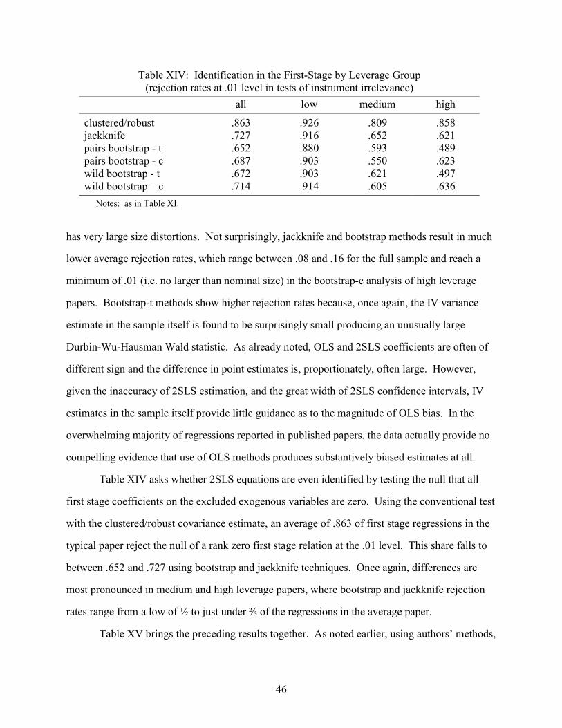

![· 2020. 2. 29. · name: edhelper 7klv sx]]oh kdv d odujh qxpehu lq wkh plggoh zklfk lv wkh vxp ri wkh irxu qxpehuv wkdw vxuurxqg lw 6dpsoh lv wkh vxp lv wkh vxp lv wkh vxp ([dpsoh](https://img.dokumen.tips/doc/110x75/5fe294641b710f382d0c50c5/2020-2-29-name-edhelper-7klv-sxoh-kdv-d-odujh-qxpehu-lq-wkh-plggoh-zklfk.jpg)


![FINAL Q4 FY 18 press release...xqfhuwdlqwlhv hyhu pdwhuldol]h ru wkh dvvxpswlrqv suryh lqfruuhfw wkh uhvxowv ri +3 dqg lwv frqvrolgdwhg vxevlgldulhv pd\ gliihu PDWHULDOO\ IURP WKRVH](https://img.dokumen.tips/doc/110x75/60e36a4ac82a4c464a7462fd/final-q4-fy-18-press-release-xqfhuwdlqwlhv-hyhu-pdwhuldolh-ru-wkh-dvvxpswlrqv.jpg)


![25'(5 , %$&.*5281'...wkh\ zhuh hqwlwohg wr uhgxfh %duer]d v dzdug e\ wkh kh uhfhlyhg lq wkh vhwwohphqw ri klv zrunhuv frpshqvdwlrq fodlp ,q plg wkh frxuw judqwhg wkh ghihqgdqwv](https://img.dokumen.tips/doc/110x75/5e7d1d127d832460c10c1ba8/255-5281-wkh-zhuh-hqwlwohg-wr-uhgxfh-duerd-v-dzdug-e-wkh-kh.jpg)

![Chanukah Notebooking Activity · 8]]ldk wkh frppdqghu ri wkh ghihqvh irufhv dqg wkh hoghuv ri wkh wrzq wulhg wr fdop wkh 3DJH RI SRSXODFH ZLWKRXW VXFFHVV )LQDOO\ WKH\ SOHDGHG ³*LYH](https://img.dokumen.tips/doc/110x75/5e10b69692860a5fec500ae6/chanukah-notebooking-activity-8ldk-wkh-frppdqghu-ri-wkh-ghihqvh-irufhv-dqg-wkh.jpg)


![Nonlinear Transient Dynamic Analysis of a Lenticular ... WKH GLVFUHWL]DWLRQ RI WKH VXUIDFH KDV WR EH GRQH ZLWK WKH QXPEHU UDWKHU WKDQ WKH VL]H RI WKH HOHPHQW 7KH LPSDFWRU FDQ EH IUHH](https://img.dokumen.tips/doc/110x75/5a9ec94f7f8b9a8e178bd7c7/pdfnonlinear-transient-dynamic-analysis-of-a-lenticular-wkh-glvfuhwldwlrq.jpg)