July 2001

NASA/CR-2001-211032

Young-Person’s Guide to Detached-Eddy Simulation Grids Philippe R. Spalart Boeing Commercial Airplanes, Seattle, Washington

The NASA STI Program Office ... in Profile

Since its founding, NASA has been dedicated to the advancement of aeronautics and space science. The NASA Scientific and Technical Information (STI) Program Office plays a key part in helping NASA maintain this important role.

The NASA STI Program Office is operated by Langley Research Center, the lead center for NASA’s scientific and technical information. The NASA STI Program Office provides access to the NASA STI Database, the largest collection of aeronautical and space science STI in the world. The Program Office is also NASA’s institutional mechanism for disseminating the results of its research and development activities. These results are published by NASA in the NASA STI Report Series, which includes the following report types:

• TECHNICAL PUBLICATION. Reports

of completed research or a major significant phase of research that present the results of NASA programs and include extensive data or theoretical analysis. Includes compilations of significant scientific and technical data and information deemed to be of continuing reference value. NASA counterpart of peer-reviewed formal professional papers, but having less stringent limitations on manuscript length and extent of graphic presentations.

• TECHNICAL MEMORANDUM.

Scientific and technical findings that are preliminary or of specialized interest, e.g., quick release reports, working papers, and bibliographies that contain minimal annotation. Does not contain extensive analysis.

• CONTRACTOR REPORT. Scientific and

technical findings by NASA-sponsored contractors and grantees.

• CONFERENCE PUBLICATION. Collected papers from scientific and technical conferences, symposia, seminars, or other meetings sponsored or co-sponsored by NASA.

• SPECIAL PUBLICATION. Scientific,

technical, or historical information from NASA programs, projects, and missions, often concerned with subjects having substantial public interest.

• TECHNICAL TRANSLATION. English-

language translations of foreign scientific and technical material pertinent to NASA’s mission.

Specialized services that complement the STI Program Office’s diverse offerings include creating custom thesauri, building customized databases, organizing and publishing research results ... even providing videos. For more information about the NASA STI Program Office, see the following: • Access the NASA STI Program Home

Page at http://www.sti.nasa.gov • E-mail your question via the Internet to

help@sti.nasa.gov • Fax your question to the NASA STI

Help Desk at (301) 621-0134 • Phone the NASA STI Help Desk at (301)

621-0390 • Write to:

NASA STI Help Desk NASA Center for AeroSpace Information 7121 Standard Drive Hanover, MD 21076-1320

National Aeronautics and Space Administration Langley Research Center Prepared for Langley Research Center Hampton, Virginia 23681-2199 under Contract NAS1-97040

July 2001

NASA/CR-2001-211032

Young-Person’s Guide to Detached-Eddy Simulation Grids Philippe R. Spalart Boeing Commercial Airplanes, Seattle, Washington

Available from: NASA Center for AeroSpace Information (CASI) National Technical Information Service (NTIS) 7121 Standard Drive 5285 Port Royal Road Hanover, MD 21076-1320 Springfield, VA 22161-2171 (301) 621-0390 (703) 605-6000

Young-Person's Guide to

Detached-Eddy Simulation Grids

Philippe R. Spalart

Boeing Commercial Airplanes

Abstract

We give the \philosophy", fairly complete instructions, a sketchand examples of creating Detached-Eddy Simulation (DES) grids fromsimple to elaborate, with a priority on external ows. Although DESis not a zonal method, ow regions with widely di�erent griddingrequirements emerge, and should be accommodated as far as possibleif a good use of grid points is to be made. This is not unique to DES.We brush on the time-step choice, on simple pitfalls, and on tools toestimate whether a simulation is well resolved.

1 Background

DES is a recent approach, which claims wide application, either in its initialform [1] or in \cousins" which we de�ne as: hybrids of Reynolds-AveragedNavier-Stokes (RANS) and Large-Eddy Simulation (LES), aimed at high-Reynolds-number separated ows [2, 3]. The DES user and experience baseare narrow as of 2001. The team in Renton and St Petersburg has beenexercising DES for about three years [1, 4, 5]; several groups have joined andprovided independent coding and validation [6, 7, 8]. The best reason forcon�dence in DES on a quantitative basis is the cylinder paper of Travin etal. [4], which also gives the more thoughtful de�nition of DES, as well as thegridding policy which was applied. The earlier NACA 0012 paper of Shur etal. [5] was also very encouraging, but it lacked grid re�nement or even muchgrid design, and tended to test the RANS and LES modes of DES separately.

Gridding is already not easy, in RANS or in LES. DES compounds thedi�culty by, �rst, incorporating both types of turbulence treatment in the

1

same �eld and, second, being directed at complex geometries. In fact a pure-LES grid for these ows with turbulent boundary layers would be at leastas challenging; fortunately, there is no use for such a grid in the near future,as the simulation would exceed the current computing power by orders ofmagnitude [1].

The target ows are much too complex, no matter how simple the ge-ometry, to provide exact solutions with which to calibrate, or even to allowexperiments so good that approaching their results is an unquestionable mea-sure of success. The inertial range and the log layer provided valid tests, butonly of the LES mode. Besides, many sources of error are present in the sim-ulations and may compensate each other, so that reducing one error sourcecan worsen the �nal answer. Here we are thinking of disagreements in the5 to 10% range. Of course, reducing the discrepancy from say 40% to 10%is meaningful; it is the step from 4% to 1% which is di�cult to establishbeyond doubt.

For these reasons, gridding guidelines will be based on physical and nu-merical arguments, rather than on demonstrations of convergence to a \right"answer. Grid convergence in LES is more subtle, or confusing, than grid con-vergence in DNS or RANS because in LES the variables are �ltered quanti-ties, and therefore the Partial Di�erential Equation itself depends on the gridspacing. The order of accuracy depends on the quantity (order of derivative,inclusion of sub-grid-scale contribution), even without walls, and the situa-tion with walls is murky except of course in the DNS limit. We do aim atgrid convergence for Reynolds-averaged quantities and spectra, but the sen-sitivity to initial conditions is much too strong to expect grid convergence ofinstantaneous �elds (except for short times with closely de�ned initial con-ditions). In DES, we are not in a position to predict an order of accuracywhen walls are involved; we cannot even produce the �ltered equation thatis being approximated. We can only o�er the obvious statement that \thefull ow �eld is �ltered, with a length scale proportional to �, which is theDES measure of grid spacing". This probably applies to any LES with wallmodeling. Nevertheless, grid re�nement is an essential tool to explore thesoundness of this or any numerical approach.

The guidelines below will appear daunting, with many regions that aredi�cult to conceptualize at �rst. The most-desirable features of these gridsappear incompatible with a single structured block, and are di�cult to ac-comodate especially in 3D. This can make DES appear too heavy. We mustkeep in mind that the approach shown here and fully implemented on the

2

tilt-rotor airfoil below is the most elaborate, and has evolved over years. Fineresults have been obtained with simpler grids, however the accuracy was notquite as good as the number of points should have allowed.

Another limitation of this write-up is that automatic grid adaptation isnot discussed. While adaptation holds the future, combining it with LES orDES is a new �eld of study. On the other hand, the discussion is not limitedto DES based on the Spalart-Allmaras (S-A) model [9]; the only impact ofusing another model could be in the viscous spacing �y+ at the wall (x2.3.1)and possibly issues at the boundary-layer edge (x2.3.2).

We note in passing that the \o�cial" value for the CDES constant (forthe S-A base model), namely 0.65, is open to revisions. DES is not verysensitive to it, which is favorable. Several partners have had better resultswith values as low as 0.25, or even 0.1. Here, \better" is largely a visual im-pression: smaller eddies, without blow-up. In some cases, the improvementcould be that the simulation now sustains unsteadiness instead of damp-ing it out. Using this kind of qualitative criterion is the state of the art,in DES and generally in LES. Spectra do illustrate the improved accuracyfrom lowered dissipation in a more quantitative manner [9]. We attributethe variations in the preferred value of CDES to di�erences in numericaldissipation. The simulation that led to 0.65 [5] used high-order centereddi�erences, whereas the ones that �t well with lower values use upwind dif-ferences, some of them as low as second-order upwind. They may well remainstable (meaning: suppress singular vortex stretching, which is physical, aswell as numerical instabilities) without any molecular or eddy viscosity inthe LES regions, making them essentially MILES (Monotonically IntegratedLES) there. However, MILES as it stands is ine�ective in the boundary layer(BL), and the simulations discussed here are not MILES overall.

Section 2 follows with guidelines, terminology, and comments, while x3 isabout pitfalls and x4 gives examples.

2 Guidelines

2.1 Terminology

The terms Euler Region, RANS Region, and LES Region will be introducedone by one, along with Viscous Region, Outer Region, Focus Region andDeparture Region. The �rst three can be seen as parent- or \super-regions",

3

ER ER

ER ER

ER ER

ER ERDR DRDR

RR

RRRR

FR

FR

FR FRFR

FRFR FR

Figure 1: Sketch of ow regions around tilt-rotor airfoil in rotor downwashduring hover.

as shown in the Table, but the pre�x \super" will be dropped. Figure 1illustrates four of these regions; the other ones (viscous regions) are too thinto sketch. A fully e�cient grid for an external ow will be designed withthese concepts in mind, but not all are strict requirements. Regions are notdistinguished by di�erent equations being applied, but by di�erent prioritiesin the grid spacing.

Super-Region Region

Euler (ER)RANS (RR) Viscous (VR)

Outer (OR)Viscous (VR)

LES (LR) Focus (FR)Departure (DR)

4

2.2 Euler Region (ER)

This region upstream and to the sides is never entered by turbulence, or byvorticity except if it is generated by shocks. It extends to in�nity and coversmost of the volume, but contains a small share of the grid points. The ERconcept also applies to a RANS calculation. Euler gridding practices prevail,with fairly isotropic spacing in the three directions, and that spacing dictatedby geometry and shocks. In an ideal adapted grid, the spacing normal to theshock would be re�ned, but we assume shock capturing. With structuredand especially C grids, there is a tendency for needlessly �ne grid spacingsto propagate from the viscous regions into the ER, which is ine�cient. Thisis mitigated by taking advantage of unstructured or multiblock capabilities.

2.3 RANS Region (RR)

This is primarily the boundary layer, including the initial separation andalso any shallow separation bubbles such as at the foot of a shock. We areassuming gridding practices typical of pure-RANS calculations. Re�nementto much �ner grids would activate LES in these regions, but here we areconsidering \natural" DES applications. The VR and OR overlap in the loglayer.

2.3.1 Viscous Region (VR)

This region is within the RANS region of a DES, and the requirements arethe same as for a full-domain RANS. In the wall-normal direction, DESwill create the standard viscous sublayer, bu�er layer, and log layer. Allare \modeled" in the sense that the time-dependence is weak (the resolvedfrequencies are much smaller than the shear rate), and does not supply anysigni�cant Reynolds stress. The �rst spacing is as dictated by the RANSmodel, about �y+ = 2 or less for S-A. The stretching ratio �yj+1=�yj shouldbe in the neighborhood of 1.25 or less for the log layer to be accurate [3].Because of this, increasing the Reynolds number by a factor of 10 requiresadding about 11 to 13 grid layers [7]. For a �rst attempt at a problem,y+ � 5 and ratio � 1:3 should be good enough. Re�nement can be doneby the usual reduction of the �rst step and of the stretching ratio. Howeververy little is typically gained by going below �y+ = 1 and �yj+1=�yj = 1:2,and in most of our studies the wall-normal spacing has been left unchanged,

5

and re�nement has taken place primarily in the LES region.In the directions parallel to the wall, RANS practices are also appropriate.

The spacing scales with the steepness of variations of the geometry and of thecompressible ow outside, as under shocks. There is little reason why it woulddi�er from the Euler spacing discussed above, except at surface singularitiessuch as steps, or the trailing edge. The spacing is not constrained in wallunits: �x+ is unlimited. Re�nement will be manual and follow a scrutiny ofthe solution, or be adaptive and follow standard detectors.

2.3.2 RANS outer region (OR)

The whole BL is treated with modeled turbulence, with no \LES content"(unsteady 3D eddies). In attached BL's, a structured grid is e�cient, andthe wall-parallel spacing makes the same requirements across the BL (unlessthere are singular wall features such as steps, slots, or breaks in slope orcurvature).

The grid normal to the wall again follows RANS practices with the spac-ing, ideally, nowhere exceeding about �=10 where � is the BL thickness. Sincesustained stretching at the 1.25 ratio gives �yj=yj � log(1:25), this impliesthat the stretching stops around y = �=2. The velocity pro�le tolerates con-tinued stretching to �y = � log(1:25) at the BL edge quite well, but the eddyviscosity has much steeper variations in the outer layer of the BL. These vari-ations are just as steep as near the wall, which is not needed from a physicalpoint of view but is a side-e�ect of the only practical way we have to deal withthe turbulence-freestream interface (the eddy viscosity needs to fall back tonear 0, and its behavior with k-� is very similar to that with S-A). Sharplyresolving the slope break of the S-A eddy viscosity at the BL edge has nophysical merit [10]; the concern is more over numerical robustness and mak-ing sure that the solution inside the BL does not \feel" the edge grid spacing.In practice, it is safer to over-estimate � than to under-estimate it, so thatthe OR often extends into the Euler Region some, and the �=10 bound isroutinely exceeded. The solver needs to tolerate the slope discontinuity andnot generate negative values.

2.4 LES regions (LR)

These regions will contain vorticity and turbulence at some point in thesimulation but are neither BL's, nor thin shear layers along which the grid

6

can be aligned (such as the slat wake over a high-lift airfoil).

2.4.1 Viscous region (VR)

The requirements are the same as in the viscous region of the RANS region,x2.3.1. Again, even though this layer is within the LES region, the wallspacing parallel to the wall is unlimited in wall units. We used values as highas �x+ = �z+ = 8; 000 in a channel, whereas typical limits when they existare of the order of 20 [7].

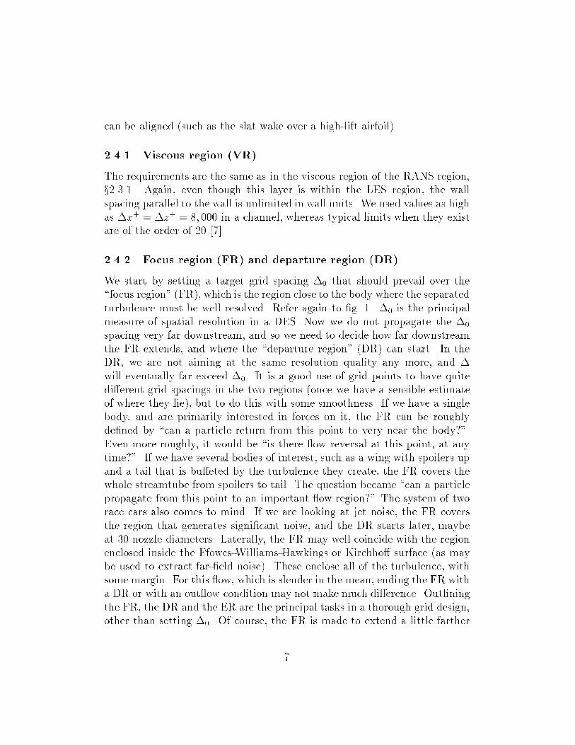
2.4.2 Focus region (FR) and departure region (DR)

We start by setting a target grid spacing �0 that should prevail over the\focus region" (FR), which is the region close to the body where the separatedturbulence must be well resolved. Refer again to �g. 1. �0 is the principalmeasure of spatial resolution in a DES. Now we do not propagate the �0

spacing very far downstream, and so we need to decide how far downstreamthe FR extends, and where the \departure region" (DR) can start. In theDR, we are not aiming at the same resolution quality any more, and �will eventually far exceed �0. It is a good use of grid points to have quitedi�erent grid spacings in the two regions (once we have a sensible estimateof where they lie), but to do this with some smoothness. If we have a singlebody, and are primarily interested in forces on it, the FR can be roughlyde�ned by \can a particle return from this point to very near the body?".Even more roughly, it would be \is there ow reversal at this point, at anytime?". If we have several bodies of interest, such as a wing with spoilers upand a tail that is bu�eted by the turbulence they create, the FR covers thewhole streamtube from spoilers to tail. The question became \can a particlepropagate from this point to an important ow region?" The system of tworace cars also comes to mind. If we are looking at jet noise, the FR coversthe region that generates signi�cant noise, and the DR starts later, maybeat 30 nozzle diameters. Laterally, the FR may well coincide with the regionenclosed inside the Ffowcs-Williams-Hawkings or Kirchho� surface (as maybe used to extract far-�eld noise). These enclose all of the turbulence, withsome margin. For this ow, which is slender in the mean, ending the FR witha DR or with an out ow condition may not make much di�erence. Outliningthe FR, the DR and the ER are the principal tasks in a thorough grid design,other than setting �0. Of course, the FR is made to extend a little farther

7

than strictly necessary for safety.The DR may smoothly evolve to spacings similar to those of the ER. It is

a beauty and a danger of DES that it is robust to grid spacings that are toocoarse for accuracy. As the grid coarsens, the DES length scale ed grows, thedestruction terms subsides, and the eddy viscosity grows [1]. The medium-and far-�eld DR may well turn into a quasi-steady RANS (the grid spacingcan rise faster than the mixing length naturally does, and the destructionterm becomes negligible). Essentially, results in the DR will not be used; itsfunction is to provide the FR with a decent \neighbor" in terms of large-scaleinviscid dynamics, better than an out ow condition could and at a modestcost.

We return to the FR, to advocate very similar grid spacings in the threedirections. Since in DES we have � = max(�x;�y;�z), the least expensiveway to obtain the desired �0 is to have cubic grid cells. This is the formulaicargument. The numerical argument is that the eddy viscosity will tend toallow steepening to about the same minimum length scale in all directions,statistically (this is away from walls, of course). As a result, �ner spacingin one or even two directions direction is wasted. The physical argument forcubic cells is that the premise of LES is to �lter out only eddies that are smallenough to be products of the energy cascade, and therefore to be statisticallyisotropic. Then, equal resolution capability in all directions is logical.

There is no unique way to choose �0. The ideal DES study containsresults with a �0, and with �0=2 (at times Rule Number 1 of DES appearsto be: \Any unsatisfactory result reported to the author is due to the user'sfailure to run on a �ne enough grid"). The cost ratio between the two runs isan order of magnitude. Still, we can provide gross �gures. LES is supposedto resolve a wide range of scales, and so a minimum of 323 would appear tobe required to cover the FR in any plausible DES, in the easiest case whenthe FR is roughly spherical. If it is elongated or if the geometry has fea-tures tangibly smaller than the diameter of the FR, even the bare minimumincreases considerably. Once we add the ER, RR and DR, it is clear thatthe minimumDES worth running includes well over 100,000 grid points (thisis over a geometry, as opposed to homogeneous or channel turbulence). Wehave run from 200,000 to 2,500,000 [4, 5, 11] and expect simulations wellbeyond 107 points in the near future.

8

2.5 Grey regions

There are intermediate zones between all regions. Most often, the boundariesare not sharp, but some are, when they correspond to block boundaries. Forinstance, over an airfoil we have started using a larger spanwise grid spacing�z in the ER and DR blocks than in the RR and FR blocks, thus savingpoints.

The boundary between the ER and any other region is placed within areasthat will never see vorticity, turbulence, or �ne scales of motion. The gridspacing may change quite a bit across that boundary, especially between FRand ER or if the RR is tight around the BL. This is also typical of RANSgrids today: even within a block, the BL and ER spacings are often designedby di�erent algorithms. Already, these calculations have an RR and an ER.

The \hand-over" from FR to DR (recall that uid normally does not owfrom the DR to the FR) can involve a sizeable coarsening in all directions.We are much less invested in the DR ow physics, and the eddy viscositywill keep the simulation stable in the DR. The same goes for any RR-to-DRboundary. This one is present in simple RANS solutions. Often, the wakeregion of a wing could fairly be described as \DR" in the sense that the gridis unable to support the wake with its accurate thickness (even a grid cutwith �ne spacing normal to the ow has no reason to be on the �nal positionof the wake). The viscous physics are neglected. None of these zones poseserious physical issues.

The RR-to-FR zone or \grey area" has always been more of a concern, inphysical terms. The grid design is not troublesome. The wall-parallel spacinghas no reason to vary wildly from RR to FR (recall that the typical owbecomes LES after separation, so that uid goes from RR to FR). If anything,a well-resolved FR may be �ner than the RR. Normally, the separation pointis not accurately known in advance. As a result, the grid design does notmark the RR-to-FR change much, if at all. It means the RR has more pointsthan needed outside the BL (as is patent in the examples below, and duepartly to structured grids), and the FR a few too many very near the wall.

The concern for this RR-to-FR zone is physical. We are expecting aswitch from 100% modeled stresses (those given by the turbulence model)to a strong dominance of the resolved stresses (those which arise from av-eraging an unsteady �eld). In other words, the RANS BL lacks any \LESContent", and we expect a new instability, freed from the wall proximity, totake over rapidly as the uid pours o� the surface. This possibility is more

9

convincing when separation is from a sharp corner or trailing edge than froma smooth surface. However, circular-cylinder results do not suggest a majorproblem [4]. The ultimate in di�culty may be reattachment after a largebubble. This all depends on: the thickness and laminar/turbulent state ofthe BL; the grid spacing, which controls which wavelengths can be resolvedand the eddy-viscosity level; the time step, which controls which frequenciescan be resolved; and �nally (physical) global instabilities which respond tocon�nement and receptivity at the separation site. Physics and numerics areintertwined, unfortunately.

We can only point out that no numerical treatment of separation andturbulence short of DNS will avoid these complexities; that user scrutiny iskey; and that grid variation is the only coherent tool to test the sensitivityof the solutions and estimate the remaining error. Once a true DES hasbeen obtained, grid re�nement has given sensible results. The present guideshould prevent the cost of grid experimentations from going out of control,as it would if all four directions were varied independently and blindly (as itis, the grid size and time step are not tied by a very rigid rule).

Note that at separation in DES we are relying on a disparity of lengthscales or \spectral gap" between the BL turbulence and the subsequent free-shear-layer turbulence. This is not the same as relying on a spectral gapover the whole separated region, which is the argument needed to advocateunsteady RANS (URANS) for massive separation. Some groups considerURANS as the answer for massively-separated ows; we consider it as am-biguous and awed and have consistent evidence that its quantitative per-formance can be quite poor [2, 5, 4].

2.6 Time step

Here we assume that the time step is chosen for accuracy, not stability. Weprimarily look at the FR, on the premise that the other regions are unlikelyto excite phenomena with higher frequency than the FR does. All the regions(and grid blocks) run with the same time step.

We consider that a sub-grid-scale model is best adjusted to allow the en-ergy cascade to the smallest eddies that can be safely tracked on the grid.Therefore, eddies with wavelengths of maybe � = 5� will be active, eventhough they cannot be highly accurate because they lack the energy cascadeto smaller eddies, and are under the in uence of the eddy viscosity instead.As a result, their transport by a reasonable di�erencing scheme (at least

10

Figure 2: DES grid over NACA 0012 airfoil.

second-order) with � = �=5 is acceptable, although not highly accurate. Allof this depends on the di�erencing scheme's performance for short waves.To best spend the computing e�ort, we wish for time-integration errors thatare of the same magnitude. Again assuming a reasonable time-integrationscheme, at least second-order, we need maybe �ve time steps per period.That leads to a local CFL number of 1. Again, it is based on rough accuracyestimates, not stability. Steps a factor of 3/2 or even 2 away in either direc-tion from this estimate cannot be described as \incorrect". Unfortunately,tests with di�erent time steps rarely give any strong indications towards anoptimal value.

We then estimate the likely highest velocity encountered in the FR, Umax,which is typically between 1.5 and several times the freestream velocity, andarrive at the time step �t = �0=Umax. It has been di�cult to con�rm orchallenge this guideline, which of course depends on the relative performanceof the spatial and temporal schemes. Orders of accuracy vary, and are of-ten higher in the spatial directions, which would push the \error-balanced"�t down somewhat. All schemes of the same order are not even createdequal. Space/time error balancing is the area that leaves the most room forexperimentation.

11

3 Pitfalls

DES produces inaccurate results if the grid is too coarse or the time step toolong, just like any other numerical strategy, but rarely \blows up". The self-adapting behavior of the eddy viscosity to the grid of course suppresses the3D Euler singularity formation (thus removing a warning of poor resolution,compared with DNS), but this feature is present in any LES and in manyRANS solvers so that there is no danger speci�c to DES. Upwind schemes,which are common, also suppress numerical divergence. If the simulation isgrossly under-resolved, a serious step of grid re�nement will trigger a largedi�erence, and thus alert the user (recall that a \serious step" implies a factorof at least

p2 and therefore nearly quadruples the cost).

An issue that is speci�c to DES is that of \ambiguous grids". It is normalDES practice for the user to signal the model whether RANS or Sub-Grid-Scale (SGS) behavior is expected in a region, and DES will respond well ifthe intermediate zones (in which the two branches of ed are close [1]) are smalland crossed rapidly by particles. This is usually the case but in our channelstudy [7], we created cases in which almost the whole domain was ambiguous.These grids were too coarse (roughly, 5 points per channel half-height h in thewall-parallel directions) for resolved turbulence to be sustained, so that thesolution was steady and there was no \resolved Reynolds stress". Howeverthe turbulence model was still limited by the grid spacing in the core region;it was on the LES branch of ed. The result was too little modeled stresscompared with the normal RANS level, and therefore skin friction. Themodel was confused. This was a contrived failure in the sense that thesegrids were visibly too coarse, the solution obviously had none of the expectedLES content, and grid re�nement would alter the results strongly enough toprompt an investigation.

We re-iterate that strongly anisotropic grids are ine�cient in the LESregion. A much �ner spacing in one direction is of no value, and may fur-thermore harm the stability of the time integration. Similarly, we need abalance between spatial and temporal steps, a balance which is more di�-cult to judge than that between spatial directions. Often, two time stepsthat are in a ratio of 2 appear equally sensible for the same ow on the samegrid.

A more subtle possibility is that DES would \fake" some e�ects thatshould be properly obtained from RANS. For instance, the e�ects of com-pressibility in a mixing layer and of rotation in a vortex are to weaken the

12

-15 -10 -5 0 5 10 15-15

-10

-5

0

5

10

15

x/D

y/D

0.0 0.5 1.0 1.5 2.0

0.0

0.5

1.0

1.5

2.0

x/D

y/D

Figure 3: DES grid over circular cylinder.

turbulence. RANS models calibrated in incompressible thin shear layers oftenmiss these e�ects, so that any reduction of the eddy viscosity steers results inthe desired direction. Reducing the eddy viscosity is precisely what DES doesrelative to RANS, so that even a DES that lacks quality resolved turbulentactivity (for instance due to inadequate spanwise domain size or resolution)could fortuitously improve results over RANS. Since demonstrating superi-ority over RANS is a recurrent theme in DES papers, there is a danger ofreporting improvements, but for a wrong reason. Note that in some RANSstudies, an eddy-viscosity reduction could also compensate for numerical dis-sipation, so that a weakened model could improve results, but then only oncoarse grids!

4 Examples

4.1 Clean airfoil over wide range of angle of attack

The grid design in our NACA 0012 study was simple, with a single block, seeFig. 2 [5]. Compared with a RANS grid adequate for an attached case, the

13

primary di�erences were the O instead of C structure and that more pointswere placed in the FR over the upper surface. However: the ER regionunder the airfoil also had a �ner grid, which was not needed; the FR cellswere not all close to cubic; no clear DR region was designed in; in particular,�z was uniform. The grid did not change with angle of attack. This wasa 141 � 61 � 25 grid with 1 chord for the spanwise period; �0 was 0:04c,dictated by �z, and the time step �t = 0:025c=U1.

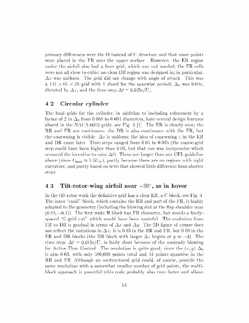
4.2 Circular cylinder

The �nal grids for the cylinder, in addition to including re�nement by afactor of 2 in �0 from 0.068 to 0.034 diameters, have several design featuresabsent in the NACA-0012 grids, see Fig. 3 [4]. The ER is clearly seen; theRR and FR are continuous; the DR is also continuous with the FR, butthe coarsening is visible. �z is uniform; the idea of coarsening z in the ERand DR came later. Time steps ranged from 0.05 to 0.035 (the coarse-gridstep could have been higher than 0.05, but that run was inexpensive whichremoved the incentive to raise �t). These are longer than our CFL guidelineabove (since Umax � 1:5U1), partly because there are no regions with tightcurvature, and partly based on tests that showed little di�erence from shortersteps.

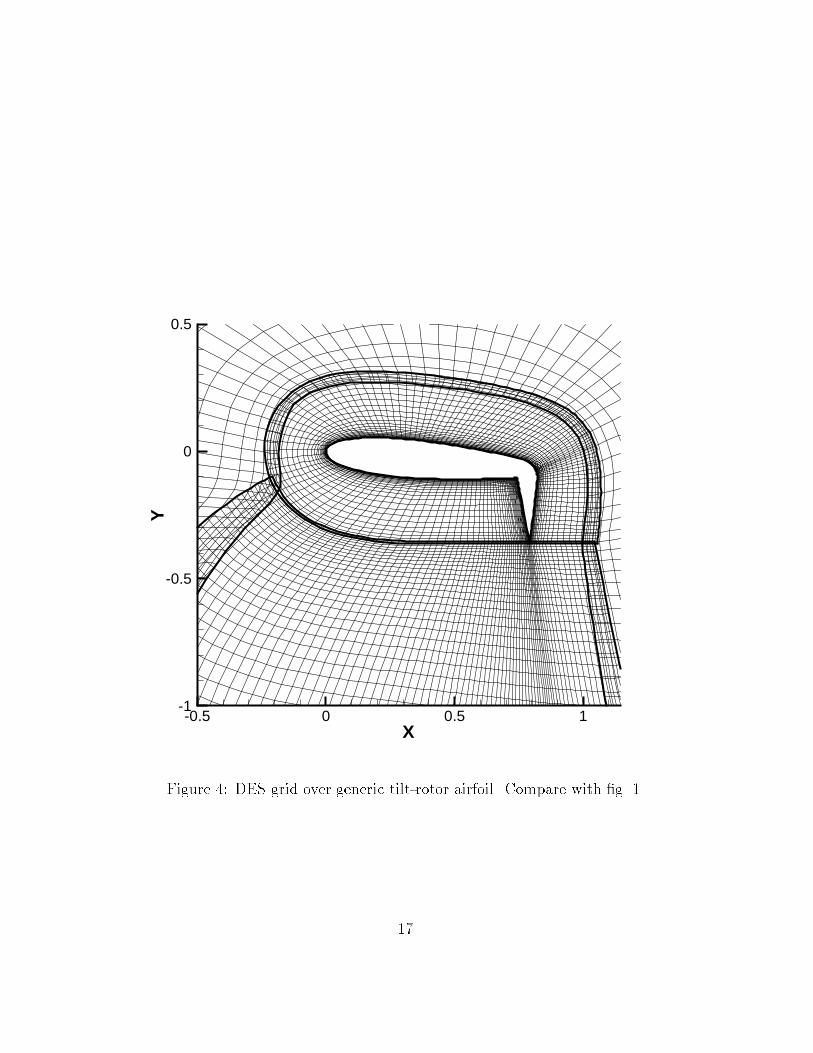
4.3 Tilt-rotor-wing airfoil near �90�, as in hover

In the tilt-rotor work the de�nitive grid has a clear ER, a C block, see Fig. 4.The inner \snail" block, which contains the RR and part of the FR, is highlyadapted to the geometry (including the blowing slot at the ap shoulder near(0:85;�0:1)). The �rst wake H block has FR character, but avoids a �nely-spaced \C-grid cut" which would have been wasteful. The evolution fromFR to DR is gradual in terms of �x and �y. The 2D �gure of course doesnot re ect the variations in �z: it is 0.03 in the RR and FR, but 0.09 in theER and DR blocks (the DR block with larger �z begins at y � �2). Thetime step, �t = 0:015c=U , is fairly short because of the unsteady blowingfor Active Flow Control. The resolution is quite good, since the (x; y) �0

is also 0.03, with only 580,000 points total and 54 points spanwise in theRR and FR. Although an unstructured grid could, of course, provide thesame resolution with a somewhat smaller number of grid points, the multi-block approach is powerful (this code probably also runs faster and allows

14

higher orders of accuracy than unstructured codes). In addition, while suchextensive multi-block grid generation is tedious, reaching the same level ofcontrol in an unstructured grid would also require very numerous steps todrive the resolution where it is desired.

4.4 Simpli�ed landing-gear truck

The landing-gear truck of Lazos, although simpli�ed, is the most completegeometry treated so far [11] (although full jet-�ghter con�gurations have beensimulated with somewhat preliminary grids but good experimental agreementby Dr. J. Forsythe at the US Air Force Academy). The grid has thirteenblocks with an RR-FR-DR-ER structure that is not as distinct as for thetilt-rotor, and about 2.5 million points. The compromises on structure wereforced by the complexity of the geometry, which made grid generation verytime-consuming.

5 Acknowledgements

All the present grids were generated and many ideas shaped by Drs. Hedges,Shur, Strelets, and Travin. Drs. Squires and Forsythe took part in manyfruitful discussions. Dr. Singer reviewed the manuscript.

References

[1] P. R. Spalart, W.-H. Jou, M. Strelets and S. R. Allmaras, \Commentson the feasibility of LES for wings, and on a hybrid RANS/LES ap-proach". 1st AFOSR Int. Conf. on DNS/LES, Aug. 4-8, 1997, Ruston,LA. In \Advances in DNS/LES", C. Liu and Z. Liu Eds., Greyden Press,Columbus, OH.

[2] P. R. Spalart, \Strategies for turbulence modelling and simulations".Int. J. Heat Fluid Flow 21, 2000, 252-263.

[3] P. R. Spalart, \Trends in turbulence treatments". AIAA-2000-2306.

[4] Travin, A., Shur, M., Strelets, M., & Spalart, P. R. 2000. \Detached-Eddy Simulations past a Circular Cylinder". Flow, Turb. Comb. 63,293-313.

15

[5] M. Shur, P. R. Spalart, M. Strelets and A. Travin, \Detached-eddysimulation of an airfoil at high angle of attack." 4th Int. Symposium onEng. Turb. Modelling and Experiments, May 24-26 1999, Corsica. W.Rodi and D. Laurence Eds., Elsevier.

[6] Constantinescu, G., and Squires, K. D., \LES and DES investigationsof turbulent ow over a sphere." AIAA-2000-0540.

[7] Nikitin, N. V., Nicoud, F., Wasistho, B., Squires, K. D., & Spalart, P.R. 2000. \An Approach to Wall Modeling in Large-Eddy Simulations".Phys Fluids 12, 7.

[8] Forsythe, J., Ho�mann, K., and Dieteker, J.-F., \Detached-eddy simu-lation of a supersonic axisymmetric base ow with an unstructured owsolver", AIAA-2000-2410.

[9] M. Strelets, \Detached eddy simulation of massively separated ows",AIAA 2001-0879.

[10] P. R. Spalart and S. R. Allmaras, \A one-equation turbulence model foraerodynamic ows," La Recherche A�erospatiale, 1, 5 (1994). Note errorin appendix for cw1.

[11] L. S. Hedges, A. Travin & P. R. Spalart 2001. \Detached-Eddy Simula-tions over a simpli�ed landing gear". To be submitted, J. Fluids Eng.

16

X

Y

-0.5 0 0.5 1-1

-0.5

0

0.5

Figure 4: DES grid over generic tilt-rotor airfoil. Compare with �g. 1.

17

X

Y

Z

Figure 5: DES grid over landing-gear truck.

18

REPORT DOCUMENTATION PAGE Form ApprovedOMB No. 0704-0188

Public reporting burden for this collection of information is estimated to average 1 hour per response, including the time for reviewing instructions, searching existing datasources, gathering and maintaining the data needed, and completing and reviewing the collection of information. Send comments regarding this burden estimate or any otheraspect of this collection of information, including suggestions for reducing this burden, to Washington Headquarters Services, Directorate for Information Operations andReports, 1215 Jefferson Davis Highway, Suite 1204, Arlington, VA 22202-4302, and to the Office of Management and Budget, Paperwork Reduction Project (0704-0188),Washington, DC 20503.

1. AGENCY USE ONLY (Leave blank) 2. REPORT DATE

July 20013. REPORT TYPE AND DATES COVERED

Contractor Report4. TITLE AND SUBTITLE

Young-Person's Guide to Detached-Eddy Simulation Grids5. FUNDING NUMBERS

RTR 706-81-13-02NAS1-97040

6. AUTHOR(S)

Philippe R. Spalart

7. PERFORMING ORGANIZATION NAME(S) AND ADDRESS(ES)

Boeing Commercial AirplanesP.O. Box 3707Seattle, WA98124

8. PERFORMING ORGANIZATIONREPORT NUMBER

9. SPONSORING/MONITORING AGENCY NAME(S) AND ADDRESS(ES)

National Aeronautics and Space AdministrationLangley Research CenterHampton, VA 23681-2199

10. SPONSORING/MONITORINGAGENCY REPORT NUMBER

NASA/CR-2001-211032

11. SUPPLEMENTARY NOTES

Prepared for Langley Research Center under Contract NAS1-97040Langley Technical Monitor: Craig Streett

12a. DISTRIBUTION/AVAILABILITY STATEMENT

Unclassified-UnlimitedSubject Category 64 Distribution: StandardAvailability: NASA CASI (301) 621-0390

12b. DISTRIBUTION CODE

13. ABSTRACT (Maximum 200 words)

We give the ``philosophy'', fairly complete instructions, a sketch and examples of creating Detached-EddySimulation (DES) grids from simple to elaborate, with a priority on external flows. Although DES is not a zonalmethod, flow regions with widely different gridding requirements emerge, and should be accommodated as faras possible if a good use of grid points is to be made. This is not unique to DES. We brush on the time-stepchoice, on simple pitfalls, and on tools to estimate whether a simulation is well resolved.

14. SUBJECT TERMS

detached-eddy simulation, DES, large-eddy simulation, LES,15. NUMBER OF PAGES

23unsteady Reynolds-averaged Navier Stokes, URANS 16. PRICE CODE

17. SECURITY CLASSIFICATIONOF REPORT

Unclassified

18. SECURITY CLASSIFICATIONOF THIS PAGE

Unclassified

19. SECURITY CLASSIFICATIONOF ABSTRACT

Unclassified

20. LIMITATIONOF ABSTRACT

UL

NSN 7540-01-280-5500 Standard Form 298 (Rev. 2-89)Prescribed by ANSI Std. Z-39-18298-102