Embed Size (px)
Citation preview

Year 8 - Openeering Special Issue

Welcome
With this special edition of the Newsletter,EnginSoft welcomes Openeering, a newbusiness unit dedicated to open sourcesoftware for engineering and appliedmathematics.
The original idea of Openeering routes backto 2008, when it became clear that, atleast in some application areas, opensource software had reached a good qualitylevel and that it was worth our time andresources to investigate it further. Sincethen, many things have happened: aninternal project was started, a dedicatedteam was selected and trained, significantbenchmarking has took place, a brand newmarketing approach has been imagined, planned andpursued.
The Openeering name comes from the words Open Sourceand Engineering, much like EnginSoft comes from thewords Engineering and Software.“Open source” and”business” look, at a first glance, an impossible pair.Software vendors may associate “open source” with “norevenues”. Software customers may associate it with “nosupport”.
Not only we believe this is not necessarily true, but, onthe contrary, we think that Open Source and commercialsource software will both play a role in the future CAE andPIDO market. For EnginSoft this vision of the future is ofcourse challenging, and we believe that competencies arethe most important weapon we and our customercompanies need to win this challenge. The business modelwe pursue is well described by Giovanni Borzi in adedicated article of this newsletter.
Scilab is the open source software with which Openeeringis starting its activity. In the last years, EnginSoft hasbecome member of the Scilab Consortium and, morerecently, started a collaboration with Scilab Enterprises asScilab Professional Partner. This new partnership certifiesthat EnginSoft has a team dedicated in providing Scilabeducation and consultancy services to industries.
“We think that the existence of Free andOpen Source software for numericalcomputation is essential. Scilab is suchsoftware.” This is what Dr. Claude Gomez,CEO of Scilab Enterprises, claims. In hisarticle, Dr. Gomez gives an insight into Scilabsoftware, its future and the developmentmodel. Gomez explains that even if Scilab isfree and open source, it is developed in aprofessional way with a Consortium of morethan twenty organizations that aresupporting and guiding Scilab’s future andpromotion.
In the last months, various real worldengineering applications have come to life
using Scilab. In the following pages, the reader can findsome of them. For example, the reader can see how Scilabcan be used for developing a finite element solver forstationary and incompressible Navier-Stokes equations orfor thermo-mechanical problems.
But Scilab is not only for finite elements solvers. In thisNewsletter, Scilab demonstrates to be extremely versatilebeing able to manage multiobjective optimizationproblems, text classification with self organizing maps(SOMs) and even being able to contribute to the weatherforecast.
To support the initiative of Openeering, a new website hasbeen created. www.openeering.com contains usefultutorials and real-case applications examples, togetherwith the Openeering SCILAB education and trainingcalendar. We take the opportunity to invite you followingour new publications on the website.
We welcome feedback, ideas and hints to improve thequality of this brand new website with the idea that itshould be, first and foremost, a website to support ourcustomers.
Together with the Openeering team, I hope you will enjoyreading this first dedicated Newsletter.
Stefano OdorizziEditor in chief
Ing. Stefano OdorizziEnginSoft CEO and President
Newsletter EnginSoft Year 8 - Openeering Special Issue - 3

6 Scilab: The Professional Free Software for Numerical Computation
9 Why Openeering
11 Scilab Finite Element Solver for stationary and incompressible Navier-Stokes equations
16 A simple Finite Element Solver for thermo-mechanical problems
21 A Simple Parallel Implementation of a FEM Solver in Scilab
26 The solution of exterior acoustic problems with Scilab
31 An unsupervised text classification method implemented in Scilab
37 Weather Forecasting with Scilab
41 Optimization? Do It with Scilab!
46 A Multi-Objective Optimization with Open Source Software
51 Scilab training courses by Openeering
Contents
SCILAB ENTERPRISES NEWS
EDUCATION AND TRAINING
SCILAB CASE STUDIES
OPENEERING
4 - Newsletter EnginSoft Year 8 - Openeering Special Issue
FEM APPLICATIONS
DATA MINING
OPTIMIZATION
PAGE 31 - AN UNSUPERVISED TEXT
CLASSIFICATION METHOD
IMPLEMENTED IN SCILAB
PAGE 21 - SCILAB FINITE ELEMENT
SOLVER FOR STATIONARY AND
INCOMPRESSIBLE NAVIER-STOKER
EQUATIONS

Newsletter EnginSoftOpeneering Special IssueTo receive a free copy of the next EnginSoft
Newsletters, please contact our Marketing office at:
All pictures are protected by copyright. Any reproduction
of these pictures in any media and by any means is
forbidden unless written authorization by EnginSoft has
been obtained beforehand.
©Copyright EnginSoft Newsletter.
AdvertisementFor advertising opportunities, please contact our
Marketing office at: [email protected]
EnginSoft S.p.A.24126 BERGAMO c/o Parco Scientifico Tecnologico
Kilometro Rosso - Edificio A1, Via Stezzano 87
Tel. +39 035 368711 • Fax +39 0461 979215
50127 FIRENZE Via Panciatichi, 40
Tel. +39 055 4376113 • Fax +39 0461 979216
35129 PADOVA Via Giambellino, 7
Tel. +39 49 7705311 • Fax 39 0461 979217
72023 MESAGNE (BRINDISI) Via A. Murri, 2 - Z.I.
Tel. +39 0831 730194 • Fax +39 0461 979224
38123 TRENTO fraz. Mattarello - Via della Stazione, 27
Tel. +39 0461 915391 • Fax +39 0461 979201
www.enginsoft.it - www.enginsoft.com
e-mail: [email protected]
COMPANY INTERESTSESTECO srl
34016 TRIESTE Area Science Park • Padriciano 99
Tel. +39 040 3755548 • Fax +39 040 3755549
www.esteco.com
CONSORZIO TCN
38123 TRENTO Via della Stazione, 27 - fraz. Mattarello
Tel. +39 0461 915391 • Fax +39 0461 979201
www.consorziotcn.it - www.improve.it
EnginSoft GmbH - Germany
EnginSoft UK - United Kingdom
EnginSoft France - France
EnginSoft Nordic - Sweden
Aperio Tecnologia en Ingenieria - Spain
www.enginsoft.com
ASSOCIATION INTERESTSNAFEMS International
www.nafems.it
www.nafems.org
TechNet Alliance
www.technet-alliance.com
RESPONSIBLE DIRECTOR
Stefano Odorizzi - [email protected]
PRINTING
Grafiche Dal Piaz - Trento
The EnginSoft NEWSLETTER is a quarterly magazine published by EnginSoft SpA Au
tori
zzaz
ione
del
Tri
buna
le d
i Tr
ento
n°
1353
RS
di d
ata
2/4/
2008
Newsletter EnginSoft Year 8 - Openeering Special Issue - 5
Via della Stazione, 27 - 38123 Mattarello di Trento
www.openeering.com
A SCILAB PROFESSIONAL PARTNER
O P E N S O U R C E E N G I N E E R I N G
Massimiliano MargonariBusiness [email protected]
Silvia PolesProduct [email protected]
Giovanni BorziProject Manager, PMP®
powered by
6 - Newsletter EnginSoft Year 8 - Openeering Special Issue
Numerical Computation: a Strategic DomainWhen engineers need to make modeling, simulation anddesign of complex systems, they usually use numericalcomputation software: this kind of tool is needed withregard to the complexity of the computation they have tomake and it can also be used for plotting andvisualization. From the software it is also possible togenerate code for embedding in real system.
With the increasing of the capabilities of computers, usingparallelism, multicore and GPU, simulating very complexsystems is now possible and numerical computations havebeen applied to a lot of domains where it was not possiblebefore to use it efficiently. So, today major scientificchallenges can be tackled in Biology, Medicine,Environment, Natural Resources and Risks, and Materials.And numerical Computation is much more efficient inindustry and service sectors such as Energy, Defense,Automotive, Aerospace, Telecommunications, Finance,Transportation and Multimedia.So, numerical computation software is strategic softwarein strategic sectors and domains. It is also used inEducation and Research. For all these reasons, we thinkthat the existence of Free and Open Source software fornumerical computation is essential. Scilab is suchsoftware.
What is Scilab?Scilab is software for numerical computation which can befreely downloaded from www.scilab.org. Binary versionsare available for Windows (XP, Vista and 7), GNU/Linuxand Mac OS X.Scilab has about 1,700 functions in many scientificdomains such as:• Mathematics.• Matrix computation, sparse matrices.• Polynomials and rational functions.• Simulation: ODE and DAE.• Classic and robust control, LMI optimization.• Differentiable and non-differentiable optimization.• Interpolation, approximation.• Signal processing.• Statistics.
It has also 2-D and 3-D graphics, with animationcapabilities.For problems where symbolic computation is needed, suchas mechanical problems, a link with Computer AlgebraSystem Maple is available.
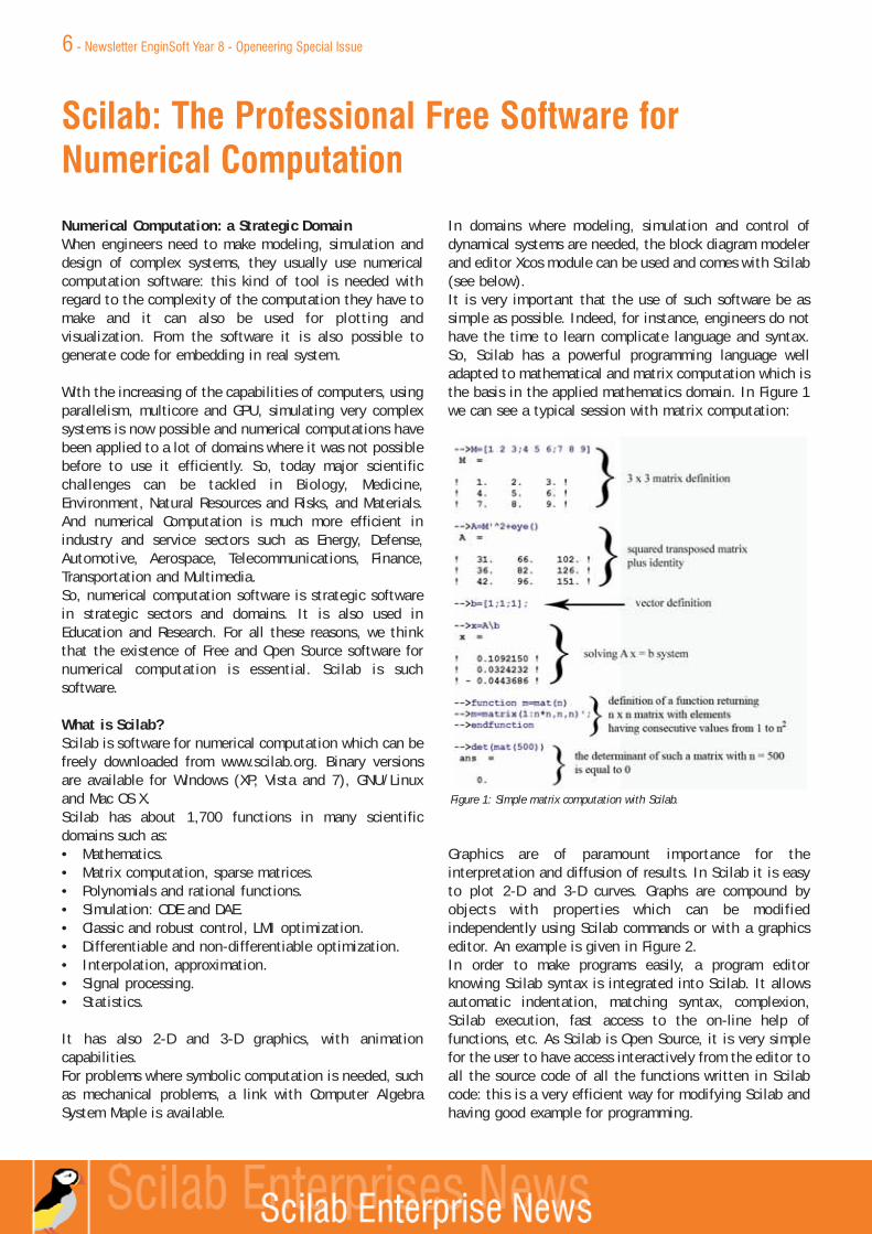
In domains where modeling, simulation and control ofdynamical systems are needed, the block diagram modelerand editor Xcos module can be used and comes with Scilab(see below).It is very important that the use of such software be assimple as possible. Indeed, for instance, engineers do nothave the time to learn complicate language and syntax.So, Scilab has a powerful programming language welladapted to mathematical and matrix computation which isthe basis in the applied mathematics domain. In Figure 1we can see a typical session with matrix computation:
Graphics are of paramount importance for theinterpretation and diffusion of results. In Scilab it is easyto plot 2-D and 3-D curves. Graphs are compound byobjects with properties which can be modifiedindependently using Scilab commands or with a graphicseditor. An example is given in Figure 2.In order to make programs easily, a program editorknowing Scilab syntax is integrated into Scilab. It allowsautomatic indentation, matching syntax, complexion,Scilab execution, fast access to the on-line help offunctions, etc. As Scilab is Open Source, it is very simplefor the user to have access interactively from the editor toall the source code of all the functions written in Scilabcode: this is a very efficient way for modifying Scilab andhaving good example for programming.
Scilab: The Professional Free Software forNumerical Computation
Figure 1: Simple matrix computation with Scilab.

Newsletter EnginSoft Year 8 - Openeering Special Issue - 7At the console level, a variable browser and an editor ofprevious commands is also available.On-line help is available for each Scilab function withexamples which can be executed directly in Scilab console.After using Scilab for a moment, the user has a lot ofwindows he has to manage. For that Scilab has a dockingsystem which allows having all the windows in a sameframe. This can be seen in Figure 2 below where theconsole is on the left, and on the right the correspondingprogram and graphics window.
In fact, Scilab is made of libraries of computationprograms in C and FORTRAN, which are linked to aninterpreter which is an interface between the programsand the user by the means of Scilab functions. Above allthe system a light and powerful Graphics User Interfaceallows the user to use Scilab easily. A large number ofScilab functions are also written in Scilab. All this Scilabinternal is summarized in the following figure. We can see on the preceding figure that it is possible for
a user to extend Scilab by adding what we call “ExternalModules”. The user has only to add FORTRAN, C, C++and/or Scilab code together with the corresponding on-line help, and to link interactively with Scilab. So, Scilab
is really an open system. Conversely, Scilab can be usedby other programs as a calculation engine.Tools for making external modules are available fromScilab Web site. For that a forge can be used. A majorimprovement of the latest releases of Scilab is theexistence of the ATOMS system which allows downloadingand installing directly from Scilab external modulesavailable in Scilab Web site: a lot of external modules arealready available. Users can create their own ATOMSmodule easily. Everything about ATOMS can be found here:
atoms.scilab.org.
What is Xcos?Scilab has powerful solvers for explicit(ODE) and implicit (DAE) differentialequation systems. So, it is possible tosimulate dynamical systems and the Xcosmodule, which is integrated into Scilab, isa block diagram graphical editor whichallows representing most of hybrid (withcontinuous and discrete time componentsand conditioning events) dynamicalsystems. It is possible to build the model ofa dynamical system by gathering blockscopied from various palettes and by linkingthem.
The connections between the input/output ports modelthe communication of data from a block to another block.The connections between the activation ports model thecommunication of information for controlling the block.Many different clocks can be used in the system.Like in Scilab, Xcos is an open system and the user canbuild blocks and gather them into new palettes.
An example of a system that we want to control by usinga hybrid observer is given in the following figure. We cansee two asynchronous clocks and two super blockscontaining other blocks representing the system and theestimator.
Scilab FutureScilab has to evolve in order to stick to the fast evolutionof the world of computers and to the everyday growingneeds of the users of numerical computation, mainlyengineers in strategic domains. For that, the strategic
Figure 2: Docking of console, editor and graphics windows.
Figure 3: Scilab internal components.
Figure 4: System to be controlled with an observer.

roadmap of Scilab can be summarized in 4 importantpoints:1. High Performance Computing: using multicore, GPU
and clusters for making parallel computations. For thatnew parallel algorithms have to be made and Scilablanguage and interpreter have to be adapted.
2. Embedded systems: generating code from Xcos andfrom Scilab code to embed into devices, cars, planes…Today this point joins the preceding because of thenew multiprocessor embedded chips.
3. Links with other scientific software, free or not. This isan important point to have Scilab be a numericalplatform that can be used in coordination with otherspecialized software. Scilab has already such links withExcel, LabVIEW and ModeFRONTIER.
4. Dedicated professional external modules.
For points 1 and 2, a brand new Scilab kernel has beenmade which will combine improved performance andmemory management together to an adaptation toparallelization and code generation. This is Scilab 6 whichwill be released at the beginning of 2012 and which willbe a major evolution of Scilab.
Scilab Development ModelScilab is software coming from research. It was conceivedat INRIA (the French Research Institute for ComputerScience and Control www.inria.fr) and a consortium hasbeen created to take in charge the development and thepromotion of Scilab. 24 organizations are members ofScilab Consortium:
Scilab Consortium is hosted by the DIGITEO Foundationuntil mid-2012 (www.digiteo.fr).The development of Scilab in the Consortium was made bya dedicated team working full time for Scilab. So, even ifScilab is Free and Open Source, and uses the help of thecommunity of users for its development, it was developedin a professional way in order to become The ProfessionalFree Software for Numerical Computation.Now that Scilab can be used in a professional way both byIndustry and Academics, delivering support, services and
making dedicated professional versions and externalmodules for Scilab are a necessary requirement for the useof Scilab. It is the reason why the Scilab EnterprisesCompany has been created to take in charge all the Scilaboperation: development of free Scilab and delivering ofservices. The corresponding development model can besummarized in figure 6.
Dr. Claude GomezCEO Scilab Enterprises
Figure 5: Members of Scilab Consortium.
Figure 6: Scilab Enterprises operation.
8 - Newsletter EnginSoft Year 8 - Openeering Special Issue
Dr. Claude Gomez was graduatedin 1977 from the École Centralede Paris. He received a Ph. D.degree in numerical analysis in1980 at the Orsay University(Paris XI).
He was a senior scientistresearcher at INRIA (The FrenchNational Institute for Research
in Computer Science and Control). He began to work innumerical analysis of partial differential equations. Thenhis main topics of interest are the links betweenComputer Algebra and Numerical Computations and hemade the Macrofort Maple package for generatingcomplete FORTRAN programs from Maple. He is involvedin the development of the Scientific Software PackageScilab since 1990. He is co-author of the Metanet toolboxfor graphs and networks optimization and he made aMaple package for generating Scilab code from Maple.
He is co-author of a book in French about ComputerAlgebra (Masson, 1995), editor and co-author of a bookin English about Scilab (Birkhäuser, 1999), and co-authorof a book in French about Scilab (Springer, 2002).
He was the leader of the Scilab Research andDevelopment team since it was created in 2003 at INRIAand he was the Director of Scilab Consortium since itsintegration in the DIGITEO foundation in 2008. Now he isthe CEO of Scilab Enterprises company and so he is incharge of all Scilab operations.
Newsletter EnginSoft Year 8 - Openeering Special Issue - 9
Why Openeering
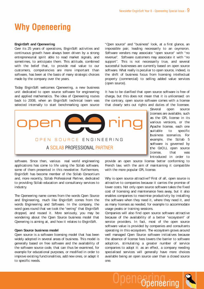
EnginSoft and OpeneeringOver its 25 years of operations, EnginSoft activities andcontinuous growth have always been driven by a strongentrepreneurial spirit able to read market signals, andsometimes, to anticipate them. This attitude, combinedwith the belief that, to provide real value to ourcustomers, competencies are more important thansoftware, has been at the basis of many strategic choicesmade by the company over the years.
Today EnginSoft welcomes Openeering, a new businessunit dedicated to open source software for engineeringand applied mathematics. The idea of Openeering routesback to 2008, when an EnginSoft technical team wasselected internally to start benchmarking open source
software. Since then, various real world engineeringapplications has come to life using the Scilab software,some of them presented in this newsletter. Furthermore,EnginSoft has become member of the Scilab Consortiumand, more recently, Scilab Professional Partner, dedicatedto providing Scilab education and consultancy services toindustry.
The Openeering name comes from the words Open Sourceand Engineering, much like EnginSoft comes from thewords Engineering and Software. In the company, theword goes round that we took the “eering” that EnginSoftdropped, and reused it. More seriously, you may bewondering about the Open Source business model thatOpenering is aiming at, and how it relates to EnginSoft.
Open Source business modelOpen source is a software licensing model that has beenwidely adopted in several areas of business. This model isgenerally based on free software and the availability ofthe software source code, that can thus be examined, forexample for educational purposes, or modified in order toimprove existing functionalities, add new ones, or adapt itto specific needs.
“Open source” and ”business” look, at a first glance, animpossible pair, leading necessarily to an oxymoron.Software vendors may associate “open source” with “norevenue”. Software customers may associate it with “nosupport”. This is not necessarily true, and severalsuccessful businesses are currently based on open sourcesoftware. What really is peculiar to open source, indeed, isthe shift of business focus from licensing intellectualproperty (commercial) to selling added value services(open source).
It has to be clarified that open source software is free ofcharge, but this does not mean that it is unlicensed: onthe contrary, open source software comes with a licensethat clearly sets out rights and duties of the licensee.
Several open sourcelicenses are available, suchas the GPL license in itsvarious versions, or theApache license, each onesuitable to specificbusiness scenarios. Forexample, the Scilab 5software is governed bythe CeCILL open sourcelicense, that wasintroduced in order to
provide an open source license better conforming toFrench law, with the aim of maintaining it compatiblewith the more popular GPL license.
Why is open source attractive? First of all, open source isattractive to companies because it carries the promise oflower costs. Not only open source software takes the fixedcost of licensing and maintenance fees away, but it alsoenables companies to maximise productivity by installingthe software when they need it, where they need it, andas many licenses as needed, for example to accommodateusage peaks or training sessions. Companies will also find open source software attractivebecause of the availability of a better “ecosystem” ofservice providers. In fact, most of the open sourcesoftware value is provided by companies and consultantsoperating in this ecosystem. The ecosystem grows aroundwell managed Open Source software initiatives becausethe absence of license fees lowers the barrier to softwareadoption, stimulating a greater number of servicecompanies to adopt it: as an effect, a company needingspecialised services will generally have more choicesavailable being an open source user than a closed sourceone.
A SCILAB PROFESSIONAL PARTNER
O P E N S O U R C E E N G I N E E R I N G

10 - Newsletter EnginSoft Year 8 - Openeering Special Issue
Furthermore, open source service providers not only canprovide education, training and support, but also morespecialised services such as customisation, that areseldom available with commercial, closed source software.
Quality and open source softwareQuality is probably the greatest challenge that opensource software have to win. Fortunately, the times ofsloppy software quality and poor developmentmanagement are behind us. Today, successful open sourcesoftware is associated with a company or consortium thattakes care of quality, non only during softwaredevelopment and integration of third partiescontributions, but also defining clear and effective market
strategy, development roadmap (including releasescheduling) and technical objectives.An example of successful quality management in the opensource software business is the Linux Ubuntu distribution,that is characterised by a clearly defined roadmap for thereleases (one every six months), the availability of longterm support releases, an extremely active community andthe possibility of purchasing commercial support from themother company, Canonical ltd. With a similarapproach, the Scilab Consortium was founded in2003 by INRIA (the French national institute forresearch in computer science and control), andhas joined the Digiteo Foundation in 2008. TheScilab Consortium plays a fundamental role inthe Scilab development, monitoring the qualityand organizing contributions to the code,keeping Scilab aligned with industry, researchand education requirements, organizing thecommunity of users, maintaining the necessaryresources and facilities, and associatingindustrial and academic partners in a powerfulinternational ecosystem. As a result, the latestScilab release was developed by a dedicatedteam working full time.
Return on investment in Open SourcesoftwareThe economical advantage of Open Source is selfevident when we try to compare the annual
cumulated costs of Scilab software with that of a closedsource competitor, in the case of an industry that isalready customer of the competitor, closed sourcesoftware. Using simple, realistic assumptions, such as that OpenSource software needs an in-depth initial training andadditional initial costs for the migration from the closedsource competitor, and not taking into account any OpenSource advantage that can’t be immediately estimated,such as a productivity increase, our conclusion is thatunder almost any condition the investment into OpenSource software will repay itself in less than two years.
The calculation details are available on thewww.openeering.com website.
The role of EnginSoft - OpeneeringPartner companies have an important role in the opensource business model. As it was previously mentioned,most of the value for the open source software users,especially for industry users, is created by partnercompanies. We believe that EnginSoft, as a leadingEuropean engineering software and services providerfocusing on technical competencies and building longterm, excellent relationships with customers, is perfectlyplaced to partner with Scilab Enterprises to bring relatededucation and services to the market.
To support the initiative a new website has been created,www.openeering.com, where useful resources arepublished, together with the Openeering SCILABeducation and training calendar.
Giovanni BorziProject manager, PMP®[email protected]

Newsletter EnginSoft Year 8 - Openeering Special Issue - 11
Scilab Finite Element Solver for stationary andincompressible Navier-Stokes equations
Scilab is an open source softwarepackage for scientific and numericalcomputing developed and freelydistributed by the Scilab Consortium.Scilab offers a high level programminglanguage which allows the user to quicklyimplement his/her own applications in asmart way, without strong programmingskills. Many toolboxes, developed by
users all over the world and made available through theinternet, represent real opportunities to create complex,efficient and multiplatform applications.Scilab is regarded almost as a clone of the well-knownMATLAB®, actually, the two technologies have many pointsin common: the programming languages are very similar(despite some differences), they both use a compiledversion of numerical libraries to make basic computationsefficient, they offer nice graphical tools and more. In brief,they adopt the same philosophy, but Scilab is completelyfree.
Unfortunately, Scilab is not yet widely used in industrialareas where, on the contrary, MATLAB® and MATLABSIMULINK® are the most known and frequently used. This isprobably due to the historical advantage that MATLAB® hasover all the competitors. Launched to the markets in the late70’s, it was the first software of its kind. However, we haveto recall that MATLAB® has many built-in functions thatScilab does not yet provide. In some cases, this could bedeterminant. While the number of Scilab users, theirexperiences and investments have grown steadily, the authorof this article thinks that the need to satisfy a larger andmore diverse market, also led to faster software
developments in recent years. As in many other cases, alsothe marketing played a fundamental role in the diffusion ofthe product.Scilab is mainly used for teaching purposes and, probably forthis reason, it is often considered inadequate for thesolution of real engineering problems. This is absolutelyfalse, and in this article, we will demonstrate that it ispossible to develop efficient and reliable solvers usingScilab, also for non trivial problems.
To this aim, we choose the Navier-Stokes equations to modela planar stationary and incompressible fluid motion. Thenumerical solution of such equations is actually considered adifficult and challenging task, as it can be seen reading [3]and [4], just to provide two references. If the user has astrong background in fluid dynamics, he/she can obviouslyimplement more complex models than the one proposed inthis document using the same Scilab platform.Anyway, there are some industrial problems that can beadequately modeled using these equations: heat exchangers,boilers and more, just to name a few possible applications.
The Navier-Stokes equations for the incompressible fluidNavier-Stokes equations can be derived applying the basiclaws of mechanics, such as the conservation and thecontinuity principles, to a reference volume of fluid (see [2]for more details). After some mathematical manipulation,the user usually reaches the following system of equations:
(1)
Fig. 2 - The benchmark problem of a laminar flow around a cylinder used to test our solver; the boundary conditions are drawn in blue. The same problem hasbeen solved using different computational strategies in [6]; the interested reader is addressed to this reference for more details.

which are known as the continuity, the momentum and theenergy equation respectively. They have to be solved in thedomain Ω, taking into account appropriate boundaryconditions. The symbols “ ·” and “ ” are used to indicatethe divergence and the gradient operator respectively, whileU, P and T are the unknown velocity vectors, the pressureand the temperature fields. The fluid properties are thedensity ρ, the viscosity µ, the thermal conductivity k andthe specific heat c which could depend generally speakingon temperature.We have to remember that in the most general caseequations, such as explained in (1), other terms such as heatsources or body forces could be involved, which we haveneglected in the present case.
For sake of simplicity we imagine all the fluid properties asconstant and we will consider, as mentioned before, only twodimensional domains. The former hypothesis represents avery important simplification because the energy equationscompletely decouple and therefore, it can be solvedseparately once the velocity field has been computed usingthe first two equations. The latter one can be easilyremoved, with some additional effort in programming.A source of difficulty is given by the first equation in (1),which represents the incompressibility constraint. In orderto satisfy the inf-sup condition (also known as Babuska-Brezzi condition) we decide to use the six-noded triangularelements; the velocity field is modeled using quadraticshape functions and two unknowns at each node areconsidered, while the pressure is modeled using linear shapefunctions and only three unknowns are used at the cornernodes. For the solution of the equations reported in (1) we decideto use a traditional Galerkin weighted residual approach,which is not ideally suitable for convection dominatedproblems: it is actually known that when the so-called Pecletnumber (which expresses the ratio between convective anddiffusion contributions) grows, the computed solution
suffers from a non-physical oscillatory behavior (see [2] fordetails). The same problem appears when dealing with theenergy equation (the third one in (1)), whenever theconvective contribution is sufficiently high.This phenomenon can uniquely be ascribed to somedeficiency of the numerical technique. For this reason, manyworkarounds have been proposed to correctly deal withconvection dominated problems. The most known are surelythe streamline upwinding schemes, the Petrov-Galerkin,least square Galerkin approaches and other stabilizationtechniques.In this work, we do not adopt any of these techniques,knowing that the computed solution with a pure Galerkin
ΔΔ
Fig. 3 - The two meshes used for the benchmark. On the top the coarse one (3486 unknowns) and on the bottom the finer one (11478 unknowns).
Fig. 4 - The sparsity pattern of the system of linear equations that have tobe solved each iteration for the solution of the first model of the channelbenchmark (3486 unknowns) is drawn. It has to be noted that the patternis symmetric with respect to the diagonal, but unfortunately the matrix isnot. The non-zero terms amount to 60294, leading to a storage requirementof 60294x(8+2*4) = 965 Kbytes, if a double precision arithmetic is used. Ifa full square matrix were used, 3486*3486*8 = 97217568 Kbytes would benecessary!
12 - Newsletter EnginSoft Year 8 - Openeering Special Issue

approach will be reliable only in the case of diffusiondominated problems. As already mentioned, it could be inprinciple possible to implement whatever technique toimprove the code and to make the solution process lesssensitive to the flow nature, but this is not the objective ofthis work.It is fundamental to note thatthe momentum equation is non-linear due to the presence ofthe advection term ρUU. Thesolution strategy adopted todeal with this nonlinearity isprobably the simplest one andit is usually known as therecursive approach (or Picardapproach).An initial guess for the velocityfield has to be provided and afirst system of linear equationscan be assembled and solved.Once the linear system has been solved the new computedvelocity field can be compared with the guess field: if nosignificant differences are found, the solution process can bestopped. Otherwise a new iteration has to be performedusing the new velocity field just computed as the guessfield.This process usually leads to the solution within areasonable amount of iterations, and it has the advantagethat it can be very easily implemented. For sure, there aremore effective techniques, such as, for example the Newton-Raphson scheme, but they usually require to compute the
Jacobian of the system hence more time for theirimplementation will be needed.
Laminar flow around a cylinderIn order to test the solver just written with Scilab, we
decided to solve a simple problem which hasbeen used by different authors (see [3], [6] forexample) as a benchmark problem to testdifferent numerical approaches for the solutionof incompressible, steady and unsteady, Navier-Stokes equations. In Figure 2 the problem isdrawn, where the geometry and the boundaryconditions can be found. The fluid density isset to 1 and the viscosity to 10-3. A parabolic (Poiseulle) velocity field in xdirection is imposed on the inlet, as shown inequation (2),
with Um=0.3, a zero pressure condition is imposed on theoutlet. The velocity in both directions is imposed to be zeroon the other boundaries. The Reynolds number is computedas Re=(¯U D)⁄ν, where the mean velocity at the inlet(¯U=(2Um)⁄3), the circle diameter D and the kinematicviscosity ν=µ⁄ρ have been used.In Figure 3 the adopted meshes have been drawn. The firsthas 809 elements, 1729 nodes, totally 3486 unknowns whilethe second has 2609 elements, 5409 nodes, totally 11478unknowns.
(2)
Fig. 5 - Starting from top, the x and y components of velocity, the velocitymagnitude and the pressure for Reynolds number equal to 20, computedwith the finer mesh.
Fig. 6 - Starting from top, the x and y components of velocity, the velocitymagnitude and the pressure for Reynolds number equal to 20, computedwith the ANSYS-Flotran solver (2375 elements, 2523 nodes).
Fig. 7 - The geometry and the boundary conditions ofthe second benchmark used to test the solver.
Newsletter EnginSoft Year 8 - Openeering Special Issue - 13

The computations can be performed on a common laptop pc.In our case, the user has to wait around 43 [sec] to solvethe first mesh, while the total solution time is around 310[sec] for the second model; in both cases 17 iterations arenecessary to reach convergence. The larger part of thesolution time is spent to compute the element contributionsand fill the matrix: this is mainly due to the fact that thesystem solution invokes the taucs, a compiled library, whilethe matrix fill-in is done directly in Scilab which isinterpreted, and not compiled, leading to a less performingrun time.The whole solution time is however always acceptable, evenfor the finest mesh.The same problem has been solved with ANSYS-Flotran (2375elements, 2523 nodes) and results can be compared with theones provided by our solver. The comparison is encouragingbecause the global behavior is well captured also with thecoarser mesh. Moreover, the numerical differences registeredbetween the maximum and minimum values are alwaysacceptable, considering thatdifferent grids are used by thesolvers.Other two quantities have beencomputed and compared with theanalogous quantities proposed in[6]. The first one is therecirculation length which is theregion behind the circle wherethe velocity along x is notpositive, whose expected value isbetween 0.0842 and 0.0852; thecoarser mesh provides a value of0.0836 and the finer one a valueof 0.0846. The second quantitywhich can be compared is thepressure drop across the circle,computed as the differencebetween the pressures in (0.15;0.20) and (0.25; 0.20); theexpected value should fallbetween 0.1172 and 0.1176. In
our case, the coarser mesh gives 0.1191 while the finer gives0.1177.
The cavity flow problemA second standard benchmark for incompressible flow isconsidered in this section. It is the flow of an isothermalfluid in a square cavity with unit sides, as schematicallyrepresented in Figure 7; the velocity field has been set tozero along all the boundaries, except for the upper one,where a uniform unitary horizontal velocity has beenimposed. In order to make the problem solvable a zeropressure has been imposed to the lower left corner of thecavity.We would like to guide the interested reader to [3], wherethe same benchmark problem has been solved. Somecomparisons between the position of the main vortexobtained with our solver and the analogous quantitycomputed by different authors and collected in [3] havebeen done and summarized in Table 1. In Figure 8 thevelocity vector (top) and magnitude (bottom) are plotted forthree different cases; the Reynolds number is computed asthe inverse of the kinematic viscosity, being the referencelength, the fluid density and the velocity all set to one. Asthe Reynolds number grows, the center of the main vortextends to move through the center of cavity.
Thermo-fluid simulation of a heat exchangerThe solver has been tested and it has been verified that itprovides accurate results for low Reynolds numbers. A newproblem, may be more interesting from an engineering pointof view, has been considered: let us imagine that a warmwater flow (density of 1000 [Kg/m3], viscosity of 5·10-4 [Pas], thermal conductivity 0.6 [W/m°C] and specific heat 4186[J/Kg°C]) with a given velocity enters into a sort of heatexchanger where some hot circles are present. We would like
Table 1 - The results collected in [3] have been reported here and comparedwith the analogous quantities computed with our solver (Scilab solver). Asatisfactory agreement is observed.
Fig. 8 - The velocity vector (top) and the velocity magnitude (bottom) plotted superimposed to the mesh forRe=100 (left), for Re=400 (center) and for Re=1000 (right). The main vortex tends to the center of the cavity asthe Reynolds numbers grows and secondary vortexes appear.
14 - Newsletter EnginSoft Year 8 - Openeering Special Issue
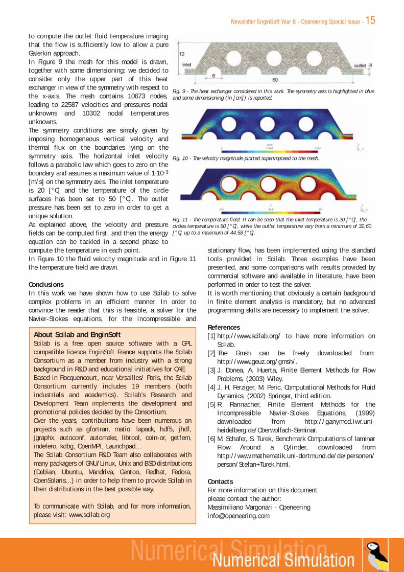
to compute the outlet fluid temperature imagingthat the flow is sufficiently low to allow a pureGalerkin approach.In Figure 9 the mesh for this model is drawn,together with some dimensioning: we decided toconsider only the upper part of this heatexchanger in view of the symmetry with respect tothe x-axis. The mesh contains 10673 nodes,leading to 22587 velocities and pressures nodalunknowns and 10302 nodal temperaturesunknowns.The symmetry conditions are simply given byimposing homogeneous vertical velocity andthermal flux on the boundaries lying on thesymmetry axis. The horizontal inlet velocityfollows a parabolic law which goes to zero on theboundary and assumes a maximum value of 1·10-3
[m/s] on the symmetry axis. The inlet temperatureis 20 [°C] and the temperature of the circlesurfaces has been set to 50 [°C]. The outletpressure has been set to zero in order to get aunique solution.As explained above, the velocity and pressurefields can be computed first, and then the energyequation can be tackled in a second phase tocompute the temperature in each point.In Figure 10 the fluid velocity magnitude and in Figure 11the temperature field are drawn.
ConclusionsIn this work we have shown how to use Scilab to solvecomplex problems in an efficient manner. In order toconvince the reader that this is feasible, a solver for theNavier-Stokes equations, for the incompressible and
stationary flow, has been implemented using the standardtools provided in Scilab. Three examples have beenpresented, and some comparisons with results provided bycommercial software and available in literature, have beenperformed in order to test the solver.It is worth mentioning that obviously a certain backgroundin finite element analysis is mandatory, but no advancedprogramming skills are necessary to implement the solver.
References[1] http://www.scilab.org/ to have more information on
Scilab.[2] The Gmsh can be freely downloaded from:
http://www.geuz.org/gmsh/.[3] J. Donea, A. Huerta, Finite Element Methods for Flow
Problems, (2003) Wiley.[4] J. H. Ferziger, M. Peric, Computational Methods for Fluid
Dynamics, (2002) Springer, third edition.[5] R. Rannacher, Finite Element Methods for the
Incompressible Navier-Stokes Equations, (1999)downloaded from http://ganymed.iwr.uni-heidelberg.de/Oberwolfach-Seminar.
[6] M. Schafer, S. Turek, Benchmark Computations of laminarFlow Around a Cylinder, downloaded fromhttp://www.mathematik.uni-dortmund.de/de/personen/person/Stefan+Turek.html.
ContactsFor more information on this document please contact the author:Massimiliano Margonari - [email protected]
Fig. 9 - The heat exchanger considered in this work. The symmetry axis is highlighted in blueand some dimensioning (in [cm]) is reported.
Fig. 10 - The velocity magnitude plotted superimposed to the mesh.
Fig. 11 - The temperature field. It can be seen that the inlet temperature is 20 [°C], thecircles temperature is 50 [°C], while the outlet temperature vary from a minimum of 32.60[°C] up to a maximum of 44.58 [°C].
About Scilab and EnginSoftScilab is a free open source software with a GPLcompatible licence EnginSoft France supports the ScilabConsortium as a member from industry with a strongbackground in R&D and educational initiatives for CAE.Based in Rocquencourt, near Versailles/ Paris, the ScilabConsortium currently includes 19 members (bothindustrials and academics). Scilab’s Research andDevelopment Team implements the development andpromotional policies decided by the Consortium. Over the years, contributions have been numerous onprojects such as gfortran, matio, lapack, hdf5, jhdf,jgraphx, autoconf, automake, libtool, coin-or, getfem,indefero, kdbg, OpenMPI, Launchpad...The Scilab Consortium R&D Team also collaborates withmany packagers of GNU/Linux, Unix and BSD distributions(Debian, Ubuntu, Mandriva, Gentoo, Redhat, Fedora,OpenSolaris...) in order to help them to provide Scilab intheir distributions in the best possible way.
To communicate with Scilab, and for more information,please visit: www.scilab.org
Newsletter EnginSoft Year 8 - Openeering Special Issue - 15
A simple Finite Element Solver for thermo-mechanical problemsIn this paper we would like to show how it is possible todevelop a simple but effective finite element solver to dealwith thermo-mechanical problems. In many engineeringsituations it is necessary to solve heat conductionproblems, both steady and unsteady state, to estimate thetemperature field inside a medium and, at the same time,compute the induced strain and stress states.To solve such problems many commercial software tools areavailable. They provide user-friendly interfaces and flexiblesolvers, which can also take into account very complicatedboundary conditions, such as radiation, and nonlinearitiesof any kind, to allow the user to model the reality in a veryaccurate and reliable way.
However, there are some situations in which the problemto be solved requires a simple and standard modeling: inthese cases it could be sufficient to have a light anddedicated software able to give reliable solutions.Moreover, other two desirable features of such a softwarecould be the possibility to access the source to easily
program new tools and, last but not least, to have a cost-and-license free product. This turns out to be very usefulwhen dealing with the solution of optimization problems.
Keeping in mind these considerations, we used the Scilabplatform and the gmsh (which are both open source codes:see [1] and [2]) to show that it is possible to buildtailored software tools, able to solve standard but complexproblems quite efficiently.
Of course, to do this it is necessary to have a goodknowledge basis in finite element formulations but nospecial skills in programming, thanks to the ease indeveloping code which characterizes Scilab.
In this paper we firstly discuss about the numericalsolution of the parabolic partial differential equationwhich governs the unsteady state heat transfer problemand then a similar strategy for the solution of elastostaticproblems will be presented. These descriptions are
absolutely general and they represent thestarting point for more complex and richermodels. The main objective of this work iscertainly not to present revolutionary results ornew super codes, but just and simply to showthat in some cases it could be feasible, usefuland profitable to develop home-madeapplications.
The thermal solverThe first step to deal with is to implement anumerical technique to solve the unsteady stateheat transfer problem described by the followingpartial differential equation:
which has to be solved in the domain Ω, takinginto account the boundary conditions, whichapply on different portions of the boundary (Γ =
ΓT U ΓQ U ΓC). They could be of Dirichlet,Neumann or Robin kind, expressing a giventemperature , a given flux or a convectioncondition with the environment:
being the unit normal vector to the boundaryand the upper-lined quantities known values at
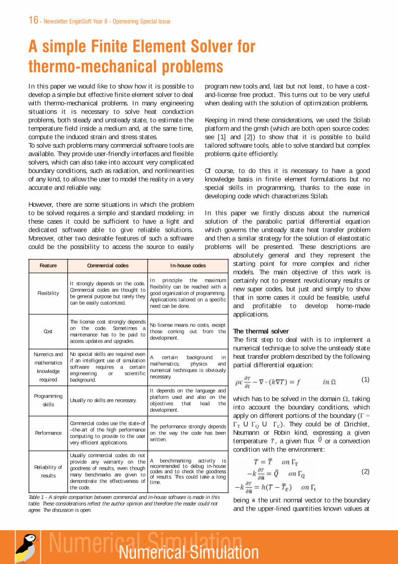
Feature Commercial codes In-house codes
Flexibility
It strongly depends on the code.Commercial codes are thought tobe general purpose but rarely theycan be easily customized.
In principle the maximumflexibility can be reached with agood organization of programming.Applications tailored on a specificneed can be done.
Cost
The license cost strongly dependson the code. Sometimes amaintenance has to be paid toaccess updates and upgrades.
No license means no costs, exceptthose coming out from thedevelopment.
Numerics and
mathematics
knowledge
required
No special skills are required evenif an intelligent use of simulationsoftware requires a certainengineering or scientificbackground.
A certain background inmathematics, physics andnumerical techniques is obviouslynecessary.
Programming
skillsUsually no skills are necessary.
It depends on the language andplatform used and also on theobjectives that lead thedevelopment.
Performance
Commercial codes use the state-of–the-art of the high performancecomputing to provide to the uservery efficient applications.
The performance strongly dependson the way the code has beenwritten.
Reliability of
results
Usually commercial codes do notprovide any warranty on thegoodness of results, even thoughmany benchmarks are given todemonstrate the effectiveness ofthe code.
A benchmarking activity isrecommended to debug in-housecodes and to check the goodnessof results. This could take a longtime.
Table 1 - A simple comparison between commercial and in-house software is made in thistable. These considerations reflect the author opinion and therefore the reader could notagree. The discussion is open.
(1)
(2)
16 - Newsletter EnginSoft Year 8 - Openeering Special Issue

each time. The symbols “ ” and “ ” are used to indicatethe divergence and the gradient operator respectively,while T is the unknown temperature field. The mediumproperties are the density ρ, the specific heat c and thethermal conductivity k which could depend, in a generalcase, on temperature. The term f on the right hand siderepresents all the body sources of heat and it could dependon both the space and time.For sake of simplicity we imagine that all the mediumproperties are constant; in this way the problem comes outto be linear, dramatically simplifying the solution.For the solution of the equations reported in (1) we decideto use a traditional Galerkin residual approach. Once adiscretization has been introduced, we obtain thefollowing expression, in matrix form:
where the symbols [.] and {.} are used to indicate matricesand vectors.A classical Euler scheme can be implemented. If we assumethe following approximation for the first time derivative ofthe temperature field:
being =[0,1] and ΔT the time step, we can rewrite, aftersome manipulation, equation (3) as:
It is well known (see [4]) that the value of the parameterplays a fundamental role. If we choose =0 an explicit
time integration scheme is obtained, actually the unknowntemperature at step n+1 can be explicitly computed
starting from already computed or known quantities.Moreover, the use of a lumped finite element approachleads to a diagonal matrix [C]; this is a desirable feature,because the solution of equation (5), which passesthrough the inversion of [C], reduces to simple and fastcomputations. The gain is much more evident if a non-linear problem has to be solved, when the inversion of [C]has to be performed at each integration step.Unfortunately, this scheme is not unconditionally stable;the time integration step Δt has actually to be less than athreshold which depend on the nature of the problem andon the mesh. In some cases this restriction could requirevery small time steps, giving high solution time.On the contrary, if =1, an implicit scheme comes out from(5), which can be specialized as:
In this case the matrix on the left involves also theconductivity contribution, which cannot be diagonalized
Figure 1 - In view of the symmetry of the pipe problem we can consider just one half of the structure during the computations. A null normal flux on the sym-metry boundary has been applied to model symmetry as on the base line (green boundaries), while a convection condition has been imposed on the externalboundaries (blue boundaries). Inside the hole a temperature is given according to the law described on the right.
Figure 2 - Temperature field at time 30 The ANSYS Workbench (left) and oursolver (right) results. A good agreement can be seen comparing these twoimages.
(3)
(4)
(5)
(6)
Newsletter EnginSoft Year 8 - Openeering Special Issue - 17

trough a lumped approach and therefore the solution of asystem of linear equations has to be computed at eachstep. The system matrix is however symmetric and positivedefinite, so a Choleski decomposition can be computedonce for all and at each integration step the backwardprocess, which is the less expensive from a computationalpoint of view, can be performed.This scheme has the great advantage to be unconditionallystable: this means that there are no restriction on the timestep to adopt. Obviously, the larger the step, the larger theerrors due to the time discretization introduced in themodel, according to (4).In principle all the intermediate values for are possible,considering that the stability of the Euler scheme isguaranteed for > 1⁄2,but usually the mostused version are the fullexplicit or implicit one.
In order to test thegoodness of ourapplication we haveperformed many testsand comparisons. Herewe present the simpleexample shown in Figure1. Let us imagine that ina long circular pipe afluid flows with atemperature whichchanges with timeaccording to the lawdrawn in Figure 1, on theright. We want to estimate the temperature distribution atdifferent time steps inside the medium and compute thetemperature of the point P.It is interesting to note that for this simple problem all theboundary conditions described in (2) have to be used. Aunit density and specific heat for the medium has beentaken, while a thermal conductivity of 5 has been chosenfor this benchmark. The environmental temperature hasbeen set to 0 and the convection coefficient to 5.
As shown in the following pictures there is a goodagreement between the results obtained with ANSYSWorkbench and our solver.
The structural solverIf we want to solve a thermo-structural problem (see [3]and references reported therein) we obviously need asolver able to deal with the elasticity equations. We focuson the simplest case, that is two dimensional problems(plane strain, plane stress and axi-symmetric problems)with a completely linear, elastic and isotropic response. Wehave to take into account that a temperature field inducesthermal deformations inside a solid medium. Actually:
where the double index i indicates that no sheardeformation can appear. The TREF represents the referencetemperature at which no deformation is produced insidethe medium.Once the temperature field is known at each time step, itis possible to compute the induced deformations and thenthe stress state.For sake of simplicity we imagine that the loads acting onthe structure are not able to produce dynamic effects andtherefore, if we neglect the body forces contributions, theequilibrium equations reduce to:
or, with the indicial notation
The elastic deformation ε can be computed as thedifference between the total and the thermal contributionsas:
which can be expressed in terms of the displacementvector field u as:
or, with the indicial notation
A linear constitutive law for the medium can be adoptedand written as:
where the matrix D will be expressed in terms of μ and λwhich describe the elastic response of the medium. Finally,after some manipulation involving equations (9), (10) and(11), one can obtain the following governing equation,which is expressed in terms of the displacements field uonly:
As usual, the above equation has to be solved togetherwith the boundary conditions, which typically are ofDirichlet (imposed displacements on Γu) or Neumannkind (imposed tractions on Γp):
Figure 3 - Temperature field in the point P plotted versus time. The ANSYSWorkbench (red) and our solver (blue) results. Also in this case a goodagreement between results is achieved.
Figure 4 - The holed plate under tensionconsidered in this work. We have takenadvantage from the symmetry withrespect to x and y axes to model only aquarter of the whole plate. Appropriateboundary conditions have been adopted,as highlighted in blue.
(7)
(8)
(9)
(10)
(11)
(12)
(13)
18 - Newsletter EnginSoft Year 8 - Openeering Special Issue

The same approachdescribed above for theheat transfer equation,the Galerkin weightedresiduals, can be usedwith equation (12) anda discretization of thedomain can beintroduced to numerically solve theproblem.Obviously, we do not need a timeintegration technique anymore,being the problem a static one. Wewill obtain a system of linearequations characterized by asymmetric and positive definitematrix: special techniques can beexploited to take advantage of theseproperties in order to reduce thestorage requirements (e.g. a sparsesymmetric storage scheme) and toimprove the efficiency (e.g. aCholeski decomposition, if a directsolver is adopted). As for the case ofthe thermal solver, many tests havebeen performed to check theaccuracy of the results. Here wepropose a classical benchmark
involving a plate of unit thickness undertension with a hole, as shown in Figure 4. Aunit Young modulus and a Poisson coefficient of0.3 have been adopted to model the materialbehavior. The vertical displacements computedwith ANSYS and our solver are compared inFigure 5: it can be seen that the two coloredpatterns are very similar and that the maximumvalues are very closed one another (ANSYS gives551.016 and we obtain 551.014). In Figure 6the tensile stress in y-direction along thesymmetry line AB is reported. It can be seenthat there is a good agreement between the
results provided by the two solvers.
Thermo-elastic analysis of a pressure vesselIn the oil-and-gas industrial sector it happens very oftento investigate the structural behavior of pressure vessels.These structures are used to contain gasses or fluids;sometimes also chemical reactions can take place insidethese devices, with a consequent growth in temperatureand pressure.
For this reason the thin shell of the vessel has to bechecked taking into account both the temperaturedistribution, which inevitably appears within the structure,and the mechanical loads. If we neglect the holes and thenozzles which could be present, the geometry of thesestructures can be viewed, very often, as a solid of
Figure 5 - The displacement in y direction computed with ANSYS (left) and our solver (right).The maximum computed values for this component are 551.016 and 551.014 respectively.
Figure 6 - The y-component of stress along the vertical symmetry line AB(see Figure 4). The red line reports the values computed with ANSYS whilethe blue one shows the results obtained with our solver. No appreciable dif-ference is present.
Figure 7 - A simple sketch illustrates the vessel considered in this work. The revolution axis is drawn withthe red dashed line and some dimensioning (in [m]) is reported. The nozzle on top is closed thanks to acap which is considered completely bonded to the structure. The nozzle neck is not covered by the insulatingmaterial. On the right the fluid temperature versus time is plotted. A pressure of 1 [MPa] acts inside thevessel.
MaterialDensity
[kg/m3]
Specific heat
[J/kg°C]
Thermal
conductivity
[W/m°C]
Young
modulus
[N/m2]
Poisson ratio
[---]
Thermalexpansion coeff.
[1/°C]
Steel 7850 434 60.5 2.0.1011 0.30 1.2.10-5
Insulation 937 303 0.5 1.1.109 0.45 2.0.10-4
Table 2 - The thermal and the mechanical properties of the materials involved in the analysis.
Newsletter EnginSoft Year 8 - Openeering Special Issue - 19
revolution. Moreover, the applied loads and the boundaryconditions reflect this symmetry and therefore it is verycommon, when applicable, to calculate a vessel using anaxi-symmetric approach.In the followings we propose a thermo-mechanical analysisof the vessel shown in Figure 7. The fluid inside the vesselhas a temperature which follows a two steps law (seeFigure 7, on the right) and a constant pressure of 1 [MPa].We would like to know which is the temperature reachedon the external surface and which is the maximum stressinside the shell, with particular attention to the upperneck.
We imagine that the vessel is made of a common steel andthat it has an external thermal insulating cover: therelevant material properties are listed in Table 2.When dealing with a thermo-mechanical problem it couldbe reasonable to use two different meshes to model andsolve the heat transfer and the elasticity equations.Actually, if in the first case we usually are interested inaccurate modeling the temperature gradients, in thesecond case we would like to have a reliable estimation ofstress peaks, which in principle could appear in differentzones of the domain. For this reason we decided to havethe possibility to use different computational grids: oncethe temperature field is known, it will be mapped on to thestructural mesh allowing in this way a better flexibility ofour solver. In the case of the pressure vessel we decided to
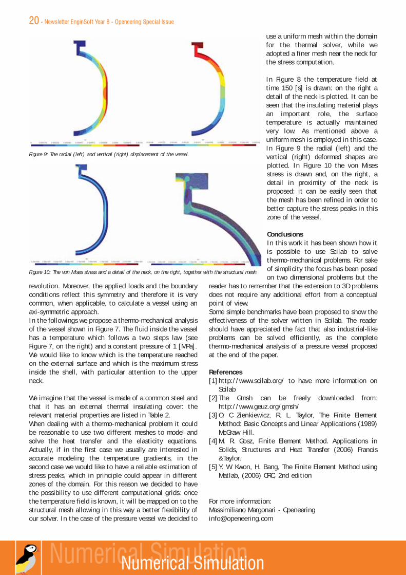
use a uniform mesh within the domainfor the thermal solver, while weadopted a finer mesh near the neck forthe stress computation.
In Figure 8 the temperature field attime 150 [s] is drawn: on the right adetail of the neck is plotted. It can beseen that the insulating material playsan important role, the surfacetemperature is actually maintainedvery low. As mentioned above auniform mesh is employed in this case.In Figure 9 the radial (left) and thevertical (right) deformed shapes areplotted. In Figure 10 the von Misesstress is drawn and, on the right, adetail in proximity of the neck isproposed: it can be easily seen thatthe mesh has been refined in order tobetter capture the stress peaks in thiszone of the vessel.
ConclusionsIn this work it has been shown how itis possible to use Scilab to solvethermo-mechanical problems. For sakeof simplicity the focus has been posedon two dimensional problems but the
reader has to remember that the extension to 3D problemsdoes not require any additional effort from a conceptualpoint of view.Some simple benchmarks have been proposed to show theeffectiveness of the solver written in Scilab. The readershould have appreciated the fact that also industrial-likeproblems can be solved efficiently, as the completethermo-mechanical analysis of a pressure vessel proposedat the end of the paper.
References[1]http://www.scilab.org/ to have more information on
Scilab[2]The Gmsh can be freely downloaded from:
http://www.geuz.org/gmsh/[3]O. C Zienkiewicz, R. L. Taylor, The Finite Element
Method: Basic Concepts and Linear Applications (1989)McGraw Hill.
[4]M. R. Gosz, Finite Element Method. Applications inSolids, Structures and Heat Transfer (2006) Francis&Taylor.
[5]Y. W. Kwon, H. Bang, The Finite Element Method usingMatlab, (2006) CRC, 2nd edition
For more information:Massimiliano Margonari - [email protected]
Figure 9: The radial (left) and vertical (right) displacement of the vessel.
Figure 10: The von Mises stress and a detail of the neck, on the right, together with the structural mesh.
20 - Newsletter EnginSoft Year 8 - Openeering Special Issue
A Simple Parallel Implementation of a FEM Solverin Scilab Nowadays many simulation software have the possibility totake advantage of multi-processors/cores computers in orderto reduce the solution time of a given task. This not onlyreduces the annoying delays typical in the past, but allows theuser to evaluate larger problems and to do more detailedanalyses and to analyze a greater number of scenarios.Engineers and scientists who are involved in simulationactivities are generally familiar with the terms “HighPerformance Computing” (HPC). These terms have been coinedto indicate the ability to use a powerful machine to efficientlysolve hard computational problems.One of the most important keywords related to the HPC iscertainly parallelism. Total execution time will be reduced ifthe original problem can be divided in a given number ofsubtasks which are then tackled concurrently, that is inparallel, by a number of cores.To completely take advantage of this strategy three conditionshave to be satisfied: the first one is that the problem we wantto solve has to exhibit a parallel nature or, in other words, itshould be possible to reformulate it in smaller problems, whichcan be solved simultaneously, whose solutions, opportunelycombined, give the solution of the original large problem.Secondly, the software has to be organized and written toexploit this parallel nature. So typically, the serial version ofthe code has to be modified where necessary to this aim.Finally, we need the right hardware to support this strategy.Of course, if one of these three conditions is not fulfilled, thebenefits could be poor or even non-existent in the worst case.It is worth to mention that not all the problems arising fromengineering can be solved effectively with a parallel approach,if their associated numerical solution procedure is intrinsicallyserial.One parameter which is usually reported in the technicalliterature to judge the goodness of a parallel implementationof an algorithm or a procedure is the so-called speedup, whichis simply defined as the ratio between the execution time ona single core machine and the same quantity on a multicoremachine (S = T1/Tp), being p the number of cores used in thecomputation. Ideally, we would like to have a speedup notlower than the number of cores: unfortunately this does nothappen mainly, but not only, because some serial operationshave to be performed during the solution. In this context it isinteresting to mention the Amdahl’s law which bounds thetheoretical speedup that can be obtained, given thepercentage of serial operations (f [0,1]) that has to beglobally performed during the run. It can be written as:
It can be easily understood that the speedup S is strongly(and badly) influenced by f rather than by p. If we imagine to
have an ideal computer with infinite number of cores (p=∞)and implement an algorithm whit just 5% of operations thathave to be performed serially (f=0.05), we get a speedup of20 as a maximum. This clearly means that it is worth to investin algorithms rather than simply increasing the number ofcores…Someone in the past has moved criticism to this law, sayingthat it is too pessimistic and unable to correctly estimate thereal theoretical speedup: in any case, we think that the mostimportant lesson to learn is that a good algorithm is muchmore important that a good machine.As said before, many commercial software propose since manyyears the possibility to run parallel solutions. With a simpleinternet search it is quite easy to find some benchmarks whichadvertize the high performances and high speedup obtainedusing various architectures and solving different problems. Allthese noticeable results are usually the result of a very hardwork of code implementation.Probably the most used communication protocols toimplement parallel programs, through opportunely providedlibraries, are the MPI (Message Passing Interface), the PVM(Parallel Virtual Machine) and the openMP (open MessagePassing): there certainly are other protocols and also variantsof the aforementioned ones, such an the MPICH2 or HPMPI,which gained the attention of the programmers for some oftheir features.As the reader has probably seen, in all the acronyms listedabove there is a letter “P”. With a bit of irony we could saythat it always stands for “problems”, in view of the difficultiesthat a programmer has to tackle when trying to implement aparallel program using such libraries. Actually, the use of theselibraries is often and only a matter for expert programmers andthey cannot be easily accessed by engineers or scientists whowant to easily cut the solution time of their applications.In this paper we would like to show that a naïve but effectiveparallel application can be implemented without a greatprogramming effort and without using any of the abovementioned protocols. We used the Scilab platform (see [1])because it is free and it provides a very easy and fast way toimplement applications: on the other hand, the fact thatScilab scripts are substantially interpreted and not compiled ispaid with a not performing code in absolute sense. It ishowever possible to rewrite all the scripts using a compiledlanguage, such as C, to get a faster run-time code. The mainobjective of this work is actually to show that it is possible toimplement a parallel application and solve large problemsefficiently (e.g.: with a good speedup) in a simple way ratherthan to propose a super-fast application.To this aim, we choose the stationary heat transfer equationwritten for a three dimensional domain together with
Newsletter EnginSoft Year 8 - Openeering Special Issue - 21

appropriate boundary conditions. A standard Galerkin finiteelement (see [4]) procedure is then adopted and implementedin Scilab in such a way as to allow a parallel execution.This represents a sort of elementary “brick” for us: morecomplex problems involving partial differential equations canbe solved starting from here, adding new features whenevernecessary.
The stationary heat transfer equationAs mentioned above, we decided to consider the stationaryand linear heat transfer problem for a three-dimensionaldomain Ω. Usually it is written as:
together with Dirichlet, Neumann and Robin boundaryconditions, which can be expressed as:
The conductivity k is considered as constant, while frepresents an internal heat source. On some portions of thedomain boundary we can have imposed temperatures , givenfluxes and also convections with an environment
characterized by a temperature and a convectioncoefficient h.The discretized version of the Galerkinformulation for the above reported equationsleads to a system of linear equations which canbe shortly written as
The matrix of coefficients [K] is symmetric,positive definite and sparse. This means that agreat amount of its terms are identically zero.The vector {T} and {F} collect the unknownnodal temperatures and nodal equivalent loads.If large problems have to be solved, itimmediately appears that an effective strategyto store the matrix terms is needed. In our casewe decided to store in memory the non-zeroterms row-by-row in a unique vector opportunelyallocated, together with their column positions:in this way we also access terms efficiently. Wedecided to not take advantage of the symmetryof the matrix (actually, only the upper or lowerpart could be stored, requiring only half as muchstorage) to simplify a little the implementation.Moreover, this allows us to potentially use thesame pieces of code without any change, for thesolution of problems which lead to a not-symmetric coefficient matrix.The matrix coefficients, as well as the knownvector, can be computed in a standard way,performing the integration of known quantitiesover the finite elements in the mesh. Without
any loss of generality, we decided to only use ten-nodedtetrahedral elements with quadratic shape functions (see [4]for more details on finite elements).The solution of the resulting system is performed through thepreconditioned conjugate gradient (PCG) (see [5] for details).In Figure 1 a pseudo-code of a classical PCG scheme isreported: the reader should observe that the solution processfirstly requires to compute the product between thepreconditioner and a given vector (*) and secondly theproduct between the system matrix and another known vector(**). This means that the coefficient matrix (and also thepreconditioner) is not explicitly required, as it is when usingdirect solvers, but it could be not directly computed andstored.This is a key feature of all the iterative solvers and wecertainly can take advantage of it, when developing a parallelcode.The basic idea is to partition the mesh in such a way that,more or less, the same number of elements are assigned toeach core (process) involved in the solution, to have a wellbalanced job and therefore to fully exploit the potentiality ofthe machine. In this way each core fills a portion of the matrixand it will be able to compute some terms resulting from thematrix-vector product, when required. It is quite clear thatsome coefficient matrix rows will be split on two or moreprocesses, since some nodes are shared by elements on
different cores.The number of overlapping rowsresulting from this stronglydepends on the way we partition(* and **) the mesh. The idealpartition produces the minimumoverlap, leading to the lessernumber of non-zero terms thateach process has to compute andstore.In other words, the efficiency ofthe solution process can dependson how we partition the mesh. Tosolve this problem, which reallyis a hard problem to solve, wedecided to use the partitionfunctionality of gmsh (see [2])which allows the user to partitiona mesh using a well knownlibrary, the METIS (see [3]),which has been explicitly writtento solve this kind of problem. Theresulting mesh partition iscertainly close to the best oneand our solver will use it whenspreading the elements to theparallel processes.An example of mesh partitionperformed with METIS is plot inFigure 3, where a car model meshis considered: the elements have
Fig. 1 - The pseudo-code for a classicalpreconditioned conjugate gradient solver. It can benoted that during the iterative solution it is requiredto compute two matrix-vector products involving thepreconditioner M (*) and the coefficient matrix K(**).
[1]
[2]
[3]
22 - Newsletter EnginSoft Year 8 - Openeering Special Issue

been drawn with different colors according to their partition.This kind of partition is obviously suitable when the problemis run on a four cores machine.As a result, we can imagine that the coefficient matrix is splitrow-wise and each portion filled by a different process runningconcurrently with the others: then, the matrix-vector productsrequired by the PCG can be again computed in parallel bydifferent processes. The same approach can be obviouslyextended to the preconditioner and to the postprocessing ofelement results.For sake of simplicity we decided to use a Jacobipreconditioner: this means that the matrix [M] in Figure 1 isjust the main diagonal of the coefficient matrix. This choiceallows us to trivially implement a parallel version of thepreconditioner but it certainly produces poor results in termsof convergence rate. The number of iterations required toconverge is usually quite high and it could be reducedadopting a more effective strategy. For this reason the solverwill be hereafter addressed to as JCG and no more as PCG.
A brief description of the solver structureIn this section we would like to briefly describe the structureof our software and highlight some key points. The Scilab5.2.2 platform has been used to develop our FEM solver: weonly used the tools available in the standard distribution (i.e.:avoiding external libraries) to facilitate the portability of theresulting application and eventually to allow a fast translationto a compiled language.A master process governs the run. It firstly reads the meshpartition, organizes data and then starts a certain number ofslave parallel processes according to the user request. At thispoint, the parallel processes read the mesh file and load theinformation needed to fill their own portion of the coefficientmatrix and known vector.Once the slave processes have finished their work the masterstarts the JCG solver: when a matrix-vector product has to becomputed, the master process asks to the slave processes tocompute their contributions which will be appropriatelysummed together by the master.When the JCG reaches the required tolerance the post-processing phase (e.g.: the computation of fluxes) isperformed in parallel by the slave processes. Thesolution ends with the writing of results in a text file.A communication protocol is mandatory to manage therun. We decided to use binary files to broadcast andreceive information from the master to the slaveprocesses and conversely.The slave processes are able to wait for the binary filesand consequently read them: once the task (e.g.: thematrix-vector product) has been performed, they writethe result in another binary file which will be read bythe master process.This way of managing communication is very simplebut certainly not the best from an efficiency point ofview: writing and reading files, even if binary ones,could take a not-negligible time. Moreover, thespeedup is certainly badly influenced by this
approach. All the models proposed in the following have beensolved on a Linux 64 bit machine equipped with 8 cores and16 Gb of shared memory. It has to be said that our solver doesnot necessarily require so powerful machines to run: the codehas been actually written and run on a common Windows 32bit dualcore notepad.
A first benchmark: the Mach 4 modelA first benchmark is proposed to test our solver: wedownloaded from the internet a funny CAD model of the Mach4 car (see the Japanese anime Mach Go Go Go), produced amesh of it and defined a heat transfer problem including allkinds of boundary conditions.
The problem has no physical nor engineering meaning: theobjective is here to have a sufficiently large and non trivial
n° of nodesn° of
tetrahedral ele-ments
n° ofunknowns
n° of nodalimposed
temperatures
511758 317767 509381 2377
n° ofcores
Analysistime[s]
Systemfill-intime[s]
JCGtime [s]
Analysisspeedup
Systemfill-in
speedup
JCG speedup
1 6960 478 5959 1.00 1.00 1.00
2 4063 230 3526 1.71 2.08 1.69
3 2921 153 2523 2.38 3.12 2.36
4 2411 153 2079 2.89 3.91 2.87
5 2120 91 1833 3.28 5.23 3.25
6 1961 79 1699 3.55 6.08 3.51
7 1922 68 1677 3.62 7.03 3.55
8 2093 59 1852 3.33 8.17 3.22
Fig. 2 - The speedup values collected in Table 2 have been plotted here against thenumber of cores.
Table 1: Some data pertaining to the Mach 4 model are proposed in thistable.
Table 2: Mach 4 benchmark. The table collects the times needed to solve themodel, to perform the system fill-in and to solve the system through theJCG. The speedup are also reported in the right part of the table.
Newsletter EnginSoft Year 8 - Openeering Special Issue - 23
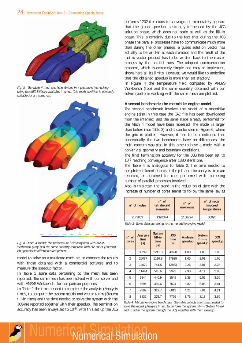
model to solve on a multicore machine, to compare the resultswith those obtained with a commercial software and tomeasure the speedup factor.In Table 1 some data pertaining to the mesh has beenreported. The same mesh has been solved with our solver andwith ANSYS Workbench, for comparison purposes.In Table 2 the time needed to complete the analysis (Analysistime), to compute the system matrix and vector terms (Systemfill-in time) and the time needed to solve the system with theJCG are reported together with their speedup. The terminationaccuracy has been always set to 10-6: with this set up the JCG
performs 1202 iterations to converge. It immediately appearsthat the global speedup is strongly influenced by the JCGsolution phase, which does not scale as well as the fill-inphase. This is certainly due to the fact that during the JCGphase the parallel processes have to communicate much morethan during the other phases: a guess solution vector hasactually to be written at each iteration and the result of thematrix vector product has to be written back to the masterprocess by the parallel runs. The adopted communicationprotocol, which is extremely simple and easy to implement,shows here all its limits. However, we would like to underlinethat the obtained speedup is more than satisfactory.In Figure 4 the temperature field computed by ANSYSWorkbench (top) and the same quantity obtained with oursolver (bottom) working with the same mesh are plotted.
A second benchmark: the motorbike engine modelThe second benchmark involves the model of a motorbikeengine (also in this case the CAD file has been downloadedfrom the internet) and the same steps already performed forthe Mach 4 model have been repeated. The model is largerthan before (see Table 3) and it can be seen in Figure 6, wherethe grid is plotted. However, it has to be mentioned thatconceptually the two benchmarks have no differences; themain concern was also in this case to have a model with anon-trivial geometry and boundary conditions.The final termination accuracy for the JCG has been set to 10-6 reaching convergence after 1380 iterations.The Table 4 is analogous to Table 2: the time needed tocomplete different phases of the job and the analysis time arereported, as obtained for runs performed with increasingnumber of parallel processes involved.Also in this case, the trend in the reduction of time with theincrease of number of cores seems to follow the same law as
Fig. 3 - The Mach 4 mesh has been divided in 4 partitions (see colors)using the METIS library available in gmsh. This mesh partition is obviouslysuitable for a 4 cores run.
Fig. 4 - Mach 4 model: the temperature field computed with ANSYSWorkbench (top) and the same quantity computed with our solver (bottom).No appreciable differences are present.
n° of nodesn° of
tetrahedral elements
n° ofunknowns
n° of nodalimposed
temperatures
2172889 1320374 2136794 36095
Table 3: Some data pertaining to the motorbike engine model.
n° ofcores
Analysistime[s]
Systemfill-intime[s]
JCGtime[s]
Analysisspeedup
Systemfill-in
speedup
JCG speedup
1 33242 2241.0 28698 1.00 1.00 1.00
2 20087 1116.8 17928 1.65 2.01 1.60
3 14679 744.5 12863 2.26 3.01 2.23
4 11444 545.6 9973 2.90 4.11 2.88
5 9844 440.9 8549 3.38 5.08 3.36
6 8694 369.6 7524 3.82 6.06 3.81
7 7889 319.7 6813 4.21 7.01 4.21
8 8832 275.7 7769 3.76 8.13 3.69
Table 4: Motorbike engine benchmark. The table collects the times needed tosolve the model (Analysis time), to perform the system fill-in (System fill-in)and to solve the system through the JCG, together with their speedup.
24 - Newsletter EnginSoft Year 8 - Openeering Special Issue

before (see Figure 5). The run with 8 parallel processes doesnot perform well because the machine has only 8 cores and westart up 9 processes (1 master and 8 slaves): this certainlywastes the performance.In Figure 7 a comparison between the temperature fieldcomputed with ANSYS Workbench (top) and our solver(bottom) is proposed. Also in this occasion no differences arepresents.
ConclusionsIn this work it has been shown how it is possible to use Scilabto write a parallel and portable application with a reasonableprogramming effort, without involving hard-to-use messagepassing protocols. The three dimensional heat transferequation has been solved through a finite element code whichtakes advantage of the parallel nature of the adoptedalgorithm: this can be seen as a sort of “elementary brick” todevelop more complicated problems. The code could berewritten with a compiled language to improve the run-timeperformance: also the message passing technique could bereorganized to allow a faster communication between the
concurrent processes, also involving different machinesconnected through a net.Stefano Bridi is gratefully acknowledged for his precious help.
References[1] http://www.scilab.org/ to have more information on
Scilab.[2] The Gmsh can be freely downloaded from:
http://www.geuz.org/gmsh/[3] http://glaros.dtc.umn.edu/gkhome/views/metis to have
more details on the METIS library.[4] O. C. Zienkiewicz, R. L. Taylor, (2000), The Finite Element
Method, volume 1: the basis. Butterworth Heimemann.[5] Y. Saad, (2003), Iterative Methods for Sparse Linear
Systems, 2nd ed., SIAM.
For more information on this document please contact theauthor: Massimiliano Margonari - [email protected]
Fig. 5 - A comparison between the speedup obtained with the twobenchmarks. The ideal speedup (the main diagonal) has been highlightedwith a black dashed line. In both cases it can be see that the speedup followthe same roughly linear trend, reaching a value between 3.5 and 4 whenusing 6 cores. The performance drastically deteriorates when involving morethan 6 cores probably because the machine where runs were performed hasonly 8 cores.
Fig. 6 - The motorbike engine mesh used for this second benchmark.
Fig. 7 - The temperature field computed by ANSYS Workbench (top) and byour solver (bottom). Also in this case the two solvers lead to the sameresults, as it can be seen looking the plots.
Newsletter EnginSoft Year 8 - Openeering Special Issue - 25

The boundary element method (shortly BEM) is a wellestablished numerical method which is known within theAcademia since the Seventies for the solution of boundaryintegral equations. It has been proposed to solve a widerange of engineering problems, ranging from structuralmechanics up to fluid mechanics, with alternating success(see [1], [2] and the reported bibliography to have moredetails on BEM).This method has been often compared to the finiteelement method (FEM) underlying, time to time, the“pros” or the “cons”. To the finite element method isrecognized a relatively “simple and scalable”mathematical approach which practically means thecapability to model a wide range of problems, includingmultiphysics and nonlinearities of any kind. On thecontrary, the BEM is generally considered to be based ona much more difficult mathematical frame, which yields toa non trivial implementation. Moreover, the range ofapplications which can be efficiently tackled with theBEM, and where the benefits are evident, is definitelysmaller with respect to the FEM.
These are probably some of the reasons why the BEM hasnot gained the attention of the software houses whichdevelop commercial simulation software for engineers.Some notable exceptions are however present in thescenario; one example is given by software dedicated tothe solution of acoustic and vibro-acoustic problems. Thereason is quite simple: it has been shown in a clearfashion that the BEM gives thepossibility to solve acousticproblems, above all those involvingunbounded domains, in a smarterand, probably, much efficient waythan the FEM.
One of the most limiting aspect of theBEM is that, being N the number ofunknowns in the model, thecomputational cost and the datastorage grow quadratic with N(shortly O(N2)) in the best case. Thisobviously represents a tremendouslimit when one tries to use thistechnique to solve industrial-likemodels, which usually arecharacterized by “large” Ns. In thelast decade a new approach, the fastmultipole method (FMM), has been
applied to the traditional BEM to mitigate this limit: theresulting approach yields to a computational cost andstorage which grow as O(N log(N)), which obviously makethe BEM much more appealing than in the past.Implementations of such approach into commercialsoftware are very recent. It is interesting to visit thewebsites of LMS international [5], FFT [6] and CYBERNETSYSTEMS [7] to just have an idea on what the marketoffers today.In this paper we present an implementation of thetraditional collocation approach for the solution ofexterior acoustic problems in Scilab. The idea is here toshow that it is possible to solve non-trivial problems in areasonable time or, better, in a time compatible with anindustrial context: to improve the global performance of
the first version of theapplication, which has beenfully written in Scilablanguage, two steps have beenperformed. Firstly, the mosttime consuming pieces of code
have been rewritten in C, compiled and linked directly inScilab; the solution time, which was really high, has beensensibly reduced thanks to this change.
Another step has been finally performed: some openMPdirectives (see [8]) have been introduced in the C routinesin order to parallelize the execution and allow to run thesimulation on a multicore shared memory machine. With
this improvement we finally get aconsistent reduction of the solutiontime.
It is important to remember that,theoretically, there is no limit in thenumber of threads that can beactivated during a run by the openMPdirectives: the real limit is due to thehardware facility used to run thesimulation.
A brief summary of the boundaryelement method (BEM) in acousticsThe Helmoltz equation is the basis oflinear acoustics. It can be used tomodel the propagation of harmonicpressure waves and it can be writtenas:
The solution of exterior acoustic problems with Scilab
Figure 1: The OpenMP logo. TheOpenMP® API specification forparallel programming.
Figure 2: The picture schematically shows a typicalexterior acoustic problem. A closed and vibratingbody, bounded by a surface Γ, is embedded in anunbounded domain Ω where the pressure wave canpropagate. The aim is to predict the pressure andthe velocity field on Γ and, potentially, in any pointof Ω.
26 - Newsletter EnginSoft Year 8 - Openeering Special Issue

in Ω (1)
where p is the complex pressure amplitude, q representsthe volume sources and k is the wave number. In this workwe imagine that the domain Ω is unbounded and thatappropriate boundary conditions (Dirichlet, Neuman andRobin) are set to the boundary Γ (see Figure 2). Equation(1) can be numerically solved by means of the FEM, whichinevitably requires to introduce a non-physical cut in theunbounded domain Ω, with a consequent violation of theSommerfeld’s radiation condition at infinity (see [2]).This means that the numerical model could suffer fromundesired spurious wave scattering, therefore producingwrong results.In literature (see [1] and [2]) we can also find an integralversion of the Helmoltz equation, which is the startingpoint for the BEM. Specifically, for exterior problems it is:
(2)
The boundary points x and y are called collocation andfield point respectively. The kernel function G is known asfundamental solution and it gives the pressure fieldinduced by a point load in an infinite space. The pressureand the velocity field are p and v; c(x) is a term whichdepends on the solid angle in x of the boundary, but italways assumes the value of 0.5 if the boundary is smooth.One interesting feature of equation (2), which isabsolutely equivalent to equation (1), is that it onlyinvolves integrals over the boundary Γ: this implies a sortof “reduction of dimensionality”, being the problemshifted from the domain Ω to the boundary Γ. Moreover,the Sommerfeld’s radiation condition is naturally satisfiedby (2) (see [2]) leading to a correct modeling of theinfinity condition.
Once the boundary has been discretized (we always adopttriangular six-noded elements), equation (2) can be“collocated” in each node (x) in the grid: it comes out asystem of linear equations which involves a fullypopulated non symmetric coefficient complex matrix, aswell as a known vector. Usually, equation (2) has to besolved as many times as the number of frequencies wewant to analyze.Very often the boundary conditions applied to Γ are all ofNeumann kind, that is the normal velocity to the boundaryis imposed, usually coming out from a previouslyperformed structural analysis. Unfortunately, the exteriorNeumann problem and the interior Dirichlet problem areself-adjoint: this means that, if equation (2) is used as itis, some non-realistic singularities in the response couldappear in proximity of the natural frequencies of thevibrating body. In the literature many numerical treatmenthave been proposed to overcome this physical non-sense.We decided to adopt the CHIEF technique (see [2]), whichsimply consists to opportunely collocate the integralequation in a certain number of fictitious points randomlypositioned inside the body.
The number of the resulting equations becomes largerthan the number of unknowns and therefore a least squaresolver is used. If the CHIEF technique is not adopted aclassical direct or iterative solver can be used.Once the pressure and the velocity fields are known on theboundary Γ it is possible to compute the same quantitiesin all the desired points x in the domain Ω, justcollocating the equation (2) and taking c(x) equal to one.Hereafter, this last phase of the analysis will be addressedto as postprocessing.
The implementation in ScilabOne of the most computationally expensive parts of a BEMcode is usually the one where the boundary integrals (see
equation (2)) are computed. Unfortunately, suchintegrals can exhibit a singular behavior, withdifferent degrees of singularity, when y approachesx. The effective numerical evaluation of theseintegrals has been the argument of discussion formany years; we are able today to estimate weaklysingular, strongly singular and hypersingularintegrals with sufficient accuracy (see [3] and thereferences) but the computations required are reallytime consuming even if an optimized coding of suchalgorithms is done.The first version of the acoustic solver has beencompletely written in Scilab scripting language andsome profiling has been done, using simplebenchmarks, to find out the most expensive parts ofthe code. One valuable feature of Scilab is thatsome integrated tools for easily profiling the scriptsare available; these tools can be used iteratively inorder to get a final optimized code in a short time.In Figure 3 the results obtained for a given
Figure 3: An example of the profiling results obtained running a simple benchmark.Thanks to the Scilab profiling tools, the most important bottlenecks in a function canbe easily found out and fixed.
Newsletter EnginSoft Year 8 - Openeering Special Issue - 27

monitored function are plotted in terms of number ofcalls, complexity and CPU time. This activity has beenfundamental to find out the most important bottlenecksin the application and remove them.As imagined, we discovered that the fill-in phase, that isthe portion of the code where the coefficient matrix isfulfilled, is characterized by a very high computationaltime. As mentioned above, the first step done to improvethe performance has been to rewrite in C the functionswhich computes the integrals, compile and link theminside Scilab. This operation which does not have requireda long time (it just consists in translating a function froma language to another) has allowed to seriously decreasethe run time.
We finally have an optimized serial version of the acousticsolver. In order to further improve the performance of ourcode we decided to use the openMP API, which allows todevelop parallel applications for multicore shared-memoryplatforms (see [8]). The fill-in phase in a boundaryelement code exhibits a parallel nature; it actuallyconsists of two nested cycles, usually the inner oneover the elements, the outer one over the boundarynodes. We decided to parallelize the inner loop, forsake of simplicity, inserting some openMP directivesinside the C routines written for the serial version.The same has been done also for the postprocessingphase, dedicated to the computation of the pressurelevel in some points located in the unboundeddomain. Also in this case we managed to reduce thesolution time, running our benchmarks on amulticore Linux machine.For the solution of the linear system of equationswe both ran a least square solver and an iterative(GMRES) solver, depending on the CHIEF techniqueis in use or not. We decided to adopt the Jacobipreconditioner for the iterative solver being thecoefficient matrix diagonal dominant, obtaining inthis way satisfactory convergence rates (see [4]).
The pulsating sphere: a first benchmarkOne of the most used benchmarks in acoustics is thepulsating sphere in the unbounded domain. For thisproblem also a closed solution is available (seeequation (3)) and therefore it is often used to provethe goodness of a specific solver or technique.The pressure level at a distance r from the spherecenter of radius R can be computed as:
(3)
being V the uniform radial velocity of the sphere, kthe wave number, ρ and c the fluid density and thespeed of sound in the fluid respectively.
We decided to firstly test the goodness of ourresults: in Figure 4 we compare the exact solution
Figure 4: The pressure level on the sphere surface obtained at different frequencies. Theexact solution (red) is compared with the numerical solution obtained with (green) andwithout (blue) the CHIEF technique.
Table 1: The table summarizes the number of boundary unknowns and thefield points used in the postprocessing in the three meshes chosen to testthe acoustic solver and its scalability.
Table 2: The table summarizes the results obtained for the three meshes (A,B and C) of different sizes used to test the performances of our acousticsolver. The fill-in, the postprocessing and the global solution time arereported, together with their speedup. The computation for a singlefrequency is considered here.
Figure 5: The solution time speedup obtained with the three models considered in thebenchmark.
28 - Newsletter EnginSoft Year 8 - Openeering Special Issue

(see equation (3)) with the numerical solution obtainedwith our solver, with and without adopting the CHIEFtechnique.
It can be seen that in both cases the exact solution is wellcaptured, except that, as expected, in proximity of theresonance frequencies of the sphere inside the consideredfrequency range. A step of 5 [Hz] has been adopted to
span the frequency range and 16 randomly generatedpoints inside the sphere volume have been used whenadopting the CHIEF approach.Secondly, we generated three different models and ranthem on a Linux machine to check the speedupperformances of our application. In Table 2 the results interms of time and speedup for different phases of the run
are collected. The Fill-in column reports the time neededto fill the linear system (matrix and known vector), thePostprocessing column reports the time required for theestimation of the pressure level in the points in thedomain while the Solution column reports the run time.Looking at results contained in Table 2 and Figure 5 itimmediately appears that the speedup deteriorates veryquickly increasing the number of threads, does not matterthe model size. This can be probably ascribed to the factthat, increasing the model size, the influence of serialportions of the code becomes not negligible with respectto the parallel ones. The speedup obtained for thepostprocessing phase is definitely better that the oneobtained for the fill-in phase; this is probably is due toour naïve openMP implementation but also to the muchmore complex task do be done.
Even though the solver does not scale extremely well ithas however to be noted that the run time is alwaysacceptable and compliant with an industrial context.
The radiated noise from an intake manifoldWe present here the results of an acoustic analysis of anintake manifold with a non trivial geometry to show thatour solver is able to also tackle industrial like problems.In Figure 7 the surface mesh adopted in the analysis isplotted. The mesh is made of 12116 surface collocationnodes, 8196 triangular quadratic elements and 9905points have been positioned to estimate the pressure levelall around the collector.
Usually, a structural analysis is firstly performed toestimate the dynamic response of the structure underexam and, in a second step, the velocity vectors, normalto the boundary of the structure, are applied as boundaryconditions to an acoustic mesh previously prepared. This“acoustic” mesh should have an adequate number ofelements / nodes to capture the desired frequenciesaccurately but without compromising too much thecomputational cost. Some commercial software haveutilities that help the user in generating such mesh and inapplying automatically the boundary conditions comingfrom the structural mesh.
This is a key feature which obviously makes the simulationprocess much easier and faster. In our case we simplydecided to modify the original CAD geometry removingsharp corners and edges knowing that this is probably notthe best way to deal with. With the modified geometry wecan produce a sufficiently smooth mesh but at a cost of alarger number of elements with respect to a moresophisticated technique. The size of the final acousticmodel is however affordable.We decided to apply different values of normal velocitiesto some patches of the boundary as Neumann boundaryconditions, keeping in mind that the obtained resultshave not any engineering meaning.
Figure 6: The pressure level computed with the model C.
Figure 7: The surface mesh of the manifold. All the corners and sharp edgesin the original CAD model have been filled in order to have a smoothsurface: in this case the c(x) term in equation (2) can be always set to 0.5.
Newsletter EnginSoft Year 8 - Openeering Special Issue - 29

We spanned the frequency range from 50 [Hz] up to 500[Hz] with a step of 5 [Hz]. In Figure 8 the computedpressure expressed in [dB] is reported for frequency 100[Hz], while in Figure 9 the acoustic pressure [Pa] is shownon a vertical plane when the manifold vibrating frequencyis 500 [Hz]. Similar outputs are obviously available for allthe computed frequencies. In Figure 10 we report thepressure versus the frequency range registered in three
different points located in the space (A, B and C) asreported in Figure 9.The analysis ran on a Linux 8 cores machine and it roughlytook 8 hours and 50 minutes.
ConclusionsIn this document we showed that it is possible to build anefficient solver for exterior acoustic problems in Scilab.Taking advantage of the possibility to add interfaces toexternal compiled libraries we decided to improve thecomputational performance of our application justrewriting in C the most expensive portions of it. Moreover,the openMP API has been used to parallelize these piecesof code and allow in this way to run the simulation onmulticore shared memory platforms, reducing, once again,the solution time.
References[1] M. Bonnet, Boundary Integral Equation Method for
Solids and Fluids, Wiley (1999).[2] S. Kirkup, The boundary element method in acoustics:
a development in Fortran, Integrated Sound Software(1998).
[3] M. Guiggiani, A. Gigante, A general algorithm formultidimensional Cauchy principal value integrals inthe boundary element method Journal of AppliedMechanics, vol 112, 906-915 (1990).
[4] Y. Saad, M.H Schultz, GMRES: a generalized minimalresidual algorithm for solving nonsymmetric linearsystems, SIAM J. Sci. Statist. Comput., 7, pp 856-869(1986).
[5] http://www.lmsintl.com/[6] http://www.fft.be/[7] http://www.cybernet.co.jp/waon/english/[8] http://openmp.org/wp/
ContactsFor more information on this document please contact theauthor:Massimiliano Margonari - [email protected]
Figure 8: The acoustic pressure expressed in [dB] estimated around themanifold when the vibrating frequency of the manifold is 100 [Hz].
Figure 9: The acoustic pressure expressed in [Pa] estimated around themanifold when the vibrating frequency of the manifold is 500 [Hz]. PointsA, B and C, are located along an horizontal radial axis (see Figure 10).
Figure 10: The acoustic pressure in [dB] versus the frequency registered inthe points A (red), B (green) and C (blue) (see Figure 9).
30 - Newsletter EnginSoft Year 8 - Openeering Special Issue

Text mining is a relatively new research field whose mainconcern is to develop effective procedures able to extractmeaningful information - with respect to a given purpose -from a collection of text documents. There are many contextswhere large amounts of documents have to be managed,browsed, explored, categorized and organized in such a waythat the information we are looking for can be accessed in afast and reliable way. Let us simply consider the internet,which is probably the largest and the most used library weknow today, to immediately understand why the interestaround text mining has increased so much during the lasttwo decades.A reliable document classification strategy can help ininformation retrieval, to improve the effectiveness of asearch engine for example, but it can be also used toautomatically understand whether an e-mail message is spamor not.The scientific literature proposes many different approachesto classify texts: it is sufficient to perform a web search tofind a large variety of papers, forums and sites discussingthis topic.The subject is undoubtedly challenging for researchers whohave to consider different and problematic aspects emergingwhen working with text documents and natural language.Usually texts are unstructured, they have different lengthsand they are written in different languages. Different authorsmeans different topics, styles, lexicons, vocabularies andjargons, just to highlight some issues. One concept can be
expressed in many different ways and, as an extreme case,also the same sentence can be graphically rendered indifferent ways:
You are welcome!U @r3 w31c0m3!
This strategy can be used to cheat the less sophisticated e-mail spam filters, which probably are not able to correctlycategorize the received message and remove it; some of themare based on simple algorithms which do not consider thereal meaning of the message but just look the words inside,one at a time.The search for an exhaustive and exact solution to the textmining problem is extremely difficult, or practicallyimpossible.Many mathematical frameworks have been developed for textclassification: naïve Bayes classifiers, supervised andunsupervised neural networks, learning vector machines andclustering techniques are just a short - and certainly notcomplete - list of possible approaches which are commonlyused in this field. They have both advantages anddisadvantages. For example, some of them usually ensure agood performance but they have to be robustly trained inadvance using predefined categories: other ones do notrequire a predefined list of categories, but they are lesseffective. For this reason the choice of the strategy is oftentailored to the specific categorization problem that has to besolved.
In spite of their differences, all of the textcategorization approaches have however afirst common problem to solve: the texthas to first processed in order to extractthe main features contained inside. Thisoperation erases the “superfluous” fromthe document, retrieving only the mostrelevant information: the categorizationalgorithm will therefore work only with aseries of features characterizing thedocument. This operation has afundamental role and it can lead tounsatisfactory results if it has not beenconducted in an appropriate way.Another crucial aspect of data miningtechniques is the postprocessing and thesummarization of results, which have tobe read and interpreted by a user.This means that the faster and the moreeffective data mining algorithm is useless
An unsupervised text classification method implemented in Scilab
Fig. 1 - This image has been generated starting from the text of the EnginSoft Flash of the Year 7 n°1issue and the tool available in [4].
Newsletter EnginSoft Year 8 - Openeering Special Issue - 31

if improperly fed or if results cannot be represented andinterpreted easily.Our personal interest for these techniques was born someweeks ago when reading the last issue of the EnginSoftnewsletter. In a typical newsletter issue there usually aremany contributions of different kinds: you probably noticedthat there are papers presenting case studies coming fromseveral industrial sectors, there are interviews, corporate andsoftware news and much more. Sometimes there are alsopapers discussing topics “strange”, for the CAE community,as probably this one may seem to be.A series of questions came out. Does the categorization usedin the newsletter respect a real structure of the documents,or is it simply due to an editorial need? Can we imagine anew categorization based on other criteria? Can we discovercategories without knowing them a-priori? Can we finallyhave a representation of this categorization? And finally, canwe have a deeper insight into our community?We decided to use the EnginSoft newsletters (see [3]) andextract from them all the articles written in English, startingfrom the first issue up to the last one. In this way we builtthe “corpus”, as it is usually called, by the text minerscommunity, the set of text documents that have to beconsidered. The first issues of the newsletter were almostcompletely written in Italian, but English contributionsoccupy the most of pages in the later years. This certainlyreflects the international growth of EnginSoft. The corpuswas finally composed of 248 plain text documents of variablelengths. The second step we performed was to set up a simpletext mining procedure to find out possible categorizations ofthe corpus, taking into account two fundamental aspects:first the fact that we do not have any a-priori categorization,and secondly the fact that the corpus cannot be consideredas “large” but, on the contrary, probably too poor to haveclear and robust results.We finally decided to use an unsupervised self organizingmap (SOM) as a tool to discover possible clusters ofdocuments. This technique has the valuable advantage of notrequiring any predefined classification and certainly ofallowing a useful and easily readable representation of acomplex dataset, through some two-dimensional plots.
The preprocessing of the corpusIt easy to understand that one of the difficulties that canarise when managing text, looking one word at a time anddisregarding for simplicity all the aspects concerning lexicon,is that we could consider as “different” words whichconceptually can have the same meaning. As an example, letus consider the following words which can appear in a text;they can be all summarized in a single word, such as“optimization”:
optimization, optimizing, optimized, optimizes, optimization, optimality.
It is clear that a good preprocessing of a text documentshould recognize that different words can be grouped under
a common root (also known as stem). This capability isusually obtained through a process referred to as stemmingand it is considered fundamental to make the text miningmore robust. Let us imagine to launch a web search enginewith the keyword “optimizing”: we probably would like thatalso documents containing the words “optimization” or“optimized” are considered when filling the results list. Thisprobably because the true objective of the search is to findout all the documents where optimization issues arediscussed.The ability of associating a word to a root is certainlydifficult to codify in a general manner. Also in this case thereare many strategies available: we decided to use the Porterstemming approach (it is one of the most used stemmingtechnique for processing English words: see the paper in [5])and apply it to all words composed by more than threeletters.If we preprocess the words listed above with the Porterstemming algorithm the result will be always the stem“optim”. It clearly does not have any meaning (we cannotfind “optim” in an English dictionary) but this does notrepresent an issue for us: we actually need “to name” in aunique way the groups of words that have the same meaning.Another ability that a good preprocessing procedure shouldhave is to remove the so-called stop words, that is, all thewords which are used to build a sentence in a correct way,according to the language rules, but that usually do notsignificantly contribute to determine the meaning of thesentence. Lists of English stop words are available on theweb and they can be easily downloaded (see [2]): theycontains words such as “and”, “or”, “for”, “a”, “an”, “the”,etc…In our text preprocessor we decided to also insert aprocedure that cuts out all the numbers, the dates and all thewords made of two letters or less; this means that words suchas “2010” or “21th” and “mm”, “f”, etc… are not considered.Also mathematical formulas and symbols are not taken intoconsideration.
Collect and manage informationThe corpus has to be preprocessed to produce a sortdictionary, which collects all the stems used by thecommunity; then, we should be able to find out all the mostinteresting information describing a document underexamation in order to characterize it.It’s worth mentioning that the dictionary resulting from theprocedure described above using the EnginSoft newsletters iscomposed of around 7000 stems. Some of them are names,surnames and acronyms such as “CAE”.
It immediately appears necessary to have a criterion to judgethe importance of a stem in a document within a corpus. Tothis purpose, we decided to adopt the so–called tf-idfcoefficient, term frequency – inverse document frequency,which takes into account both the relative frequency of astem in a document and the frequency of the stem within thecorpus. It is defined as:
32 - Newsletter EnginSoft Year 8 - Openeering Special Issue

being
where the subscripts w and d stand for a given word and agiven document respectively in the corpus C - done by Ndocuments - while ni,j represents the number of times that theword i appears in the j-th document. This coefficient allowsus to translate words into numbers.In Figure 2, the corpus has been graphically represented,plotting the matrix containing the non-zero tf-idf
coefficients computed for each stem, listedin columns, as they appear while processingthe documents, listed in rows. The strangeprofile of the non-zero coefficients in thematrix is obviously due to this fact: it isinteresting to see that the most used stemsappear early on while processing documents,and that the rate of dictionary growth - thatis the number of new stems that are addedto the dictionary by new documents - tendsto gradually decrease. This trend does notdepend, on average, on the order used indocument processing: the resulting matrix isalways denser in the left part and sparser on
the lower-right part.Obviously, the top-rightcorner is always void.The matrix in Figure 2represents a sort ofdatabase which can beused to accomplish adocument search,according to a givencriterion; for example, if
we wanted to find out the most relevant documents withrespect to the “optimization” topic, we should simply lookfor the documents corresponding to the highest tf-idf of thestem optim. The results of this search are collected in Table1, where the first 5 documents are listed.In Table 2 we list the stems which register the highest andthe lowest (non zero) tf-idf in the dictionary, together withthe documents where they appear. More generally, it isinteresting to see that high values of tf-idf are obtained bywords that appear frequently in a short document, but thatglobally are not used at all (see the acronym “VPS”). On thecontrary, low values of this coefficient are obtained bycommon words in the corpus (see “design”) that areinfrequently used in long documents.In Figure 3 the histogram of the tf-idf coefficient and theempirical cumulate density function are plotted. It can beseen that the distribution is strongly left-skewed: this meansthat there are many stems that are largely used in the corpus,therefore having very low values of tf-idf. For this reason thelogarithmic scale is preferred in order to have a betterrepresentation of the data.
A text classification using Self Organizing MapsSelf Organizing Maps (SOMs) are neural networks which havebeen introduced by Teuvo Kohonen (we address theinterested reader to [6] to have a complete review of SOMs).One of the most valuable characteristics of such maps iscertainly the fact that they allow a two-dimensionalrepresentation of multivariate datasets, preserving theoriginal topology; this means that the map does not alter thedistances between records in the original space whenprojecting them in the two-dimensional domain. For thisreason they can be used to navigate multidimensional
Document title Published inthe Newsletter
tf-idf of stem“optim”
The current status of research and applications inMultiobjective Optimization.
Year 6, issue 2 0.0082307
Multi-objective optimization for antenna design. Year 5, issue 2 0.0052656
Third International Conference on MultidisciplinaryDesign Optimization and Applications.
Year 6, issue 3 0.0050507
modeFRONTIER at TUBITAK-SAGE in Turkey. Year 5, issue 3 0.0044701
Optimal Solutions and EnginSoft announce DistributionRelationship for Sculptor Software in Europe.
Year 6, issue 3 0.0036246
Document title Published inthe Newsletter Stem tf-idf
VirtualPaintShop.Simulation of paint processes of car bodies.
Year 2, issue 4 VPSMax
0.0671475
Combustion Noise Prediction in a Small Diesel EngineFinalized to the Optimization of the Fuel Injection Strategy
Year 7, issue 3 designMin (non-zero)
0.0000261
Table 1 - The results of the search for “optimization” in the corpus using the tf-idf coefficient.
Table 2 - The stem with the maximum and the minimum (non zero) tf-idf respectively found in the corpus are reported inthe table together with the document title where they appear.
Fig. 2 - A matrix representation of the non-zeros tf-idf coefficients withinthe corpus. The matrix rows collect the text files sorted in the same order asthey are processed, while the columns collect the stems added to the dictio-nary in the same order as they appear while processing the files.
Newsletter EnginSoft Year 8 - Openeering Special Issue - 33

datasets and to detect groups of records, if present. A secondinteresting characteristic of these maps is that they arebased on an unsupervised learning: this is the reason why,sometimes, such maps are said to learn from theenvironment. They do not need any imposed categorizationnor classification of data to run, but they simply project thedataset “as it is”. The mathematical algorithm behind thesemaps is not really difficult to understand and therefore is notdifficult to implement; however, the results have to begraphically represented in such a way that they can be easilyaccessed by the user. This is probably the most difficult taskwhen developing as SOM: fortunately Scilab has a large set ofgraphical functions which can be called upon to buildcomplex outputs, such the one in Figure 6.A common practice is to use a sort of honey-combrepresentation of the map, where each hexagon stands for aneuron: colors and symbols are used to draw a result (e.g. adataset component or the number of records in a neuron).The user has to set the dimensions of the map, choosing thenumber of neurons along the horizontal and the verticaldirections (see Table 3, where the set up of our SOM is brieflyreported) and the number of training cycles that have to beperformed. Each neuron has a prototype vector (that is avector with the same dimension of the designs in thedataset) which should be representative, once the net hasbeen trained, of all the designs pertaining to that neuron.Certainly the easiest way to initialize the prototypes is tochoose random values for all their components, as we did inour case.The training consists of two phases: the first one is called“rough phase”, the second one “fine tuning” and they usuallyhave to be done with slightly different set-ups to obtain thebest training, but operationally, they do not present anydifference.During the training a design is submitted to the net andassigned to the neuron whose prototype vector is closest tothe design itself; then, the prototypes of the neurons in theneighborhood are updated trough an equation which rulesthe strength of the changes according, for example, to thetraining iteration number and to the neuron distances.During a training cycle all the designs have to be passed to
the net, always following for example a different order ofsubmission, to ensure a more robust training. There is a largevariety of rules for updating available in the literature whichcan be adopted according to the specific problem. Wedecided to use a Gaussian training function with a constantlearning factor which is progressively damped with theiteration number. This leads to a net which progressively“freezes” to a stable configuration, which should be seen asthe solution of a nonlinear projection problem of amultivariate dataset on a two dimensional space.At the end of the training phase, each design in the datasethas a reference neuron and each prototype vector shouldsummarize at best the designs in their neuron. For thisreason the prototype vectors can be thought as a “summary”of the original dataset and used to graphically renderinformation through colored pictures.One of the most frequent criticism to SOMs that we hearwithin the engineering community is that these maps do notprovide, as a result, any number but rather colored picturesthat only “gurus” can interpret. All this, and the fact thatresults often depend on the guru who reads the map,confuses engineers. We are pretty convinced that this is awrong feeling; these maps, and consequently the coloredpictures used to present results, are obtained with a precisealgorithm such those used in other fields. As an example, letus remember that even results coming from a finite elementsimulation of a physical phenomenon are usually presentedthrough a plot (e.g.: stress, velocity or pressure fields in adomain) and that they can change as the model set upchanges (e.g.: mesh, time integration step…) and thattherefore they have to be always interpreted by a skilledengineer.We submitted the dataset with the tf-idf coefficients and ranan SOM training with the setup summarized in Table 3. Toprevent stems with too high or too low values playing a rolein the SOM training, we decided to keep only those belongingto the interval [0.0261 - 2.6484]·10-3. This interval has beenchosen starting from the empirical cumulative distributionreported in Figure 3 and looking for the tf-idf correspondingto the 0.1 and the 0.8 probability respectively. In this way,the extremes, which could be due, for example, to spelling
Fig. 3 - The histogram (left) and the empirical cumulative distribution (right) of the tf-idf. The distribution has clearly a high skewness: the large majority ofstems has a low tf-idf. For this reason the logarithmic scale has been used in the graphs.
34 - Newsletter EnginSoft Year 8 - Openeering Special Issue

mistakes, are cancelled out from the dataset, ensuring a morerobust training. The dictionary decreases from 7000 toaround 5000 stems, which are considered to be enough todescribe exhaustively the corpus, keeping very commonwords and preserving the peculiarities of documents.Once the SOM has been trained (in Figure 4 the quantizationerror versus the training iteration is drawn), we decided touse the “distance matrix” as the best tool to “browse” theresults. The so-called D-matrix is a plot of the net where thecolor scale is used to represent the mean distance betweenthe neurons’ prototype vector and their neighbors (red means“far”, blue means “close”). In this way, with just a glance,one can understand how the dataset is distributed on thenet, and also detect clusters of data, if any. This graphicaltool can be also enriched with other additional information,plotted together with thecolor scale, making itpossible to represent thedataset in a more usefulway. An example of theseenriched versions is givenin Figures 5 and 6.Looking at the plot of theD-matrix reported inFigure 5, one canconclude that there aremainly two large groupsof papers (the two bluezones), which are nothowever sharplyseparated, and there aremany outliers. It is noteasy to identify in aunique way other clustersof papers, since thedistance is too high
between neurons’ prototypes outside theblue zones.The dimension of the white diamondssuperimposed on the neurons isproportional to the number of documentswhich pertains to the neuron. It is clearthat there are many files that fall intoone of these two groups.
Looking to the map drawn in Figure 6, we can try tounderstand what is the main subject discussed by papers inthese groups. We decided to report the stems which gain thehighest tf-idf in the prototype vectors, providing in this waytwo “keywords” that identify papers falling in the neurons. Inthe first group, positioned on the left-upper part of the map,certainly there are documents discussing EnginSoft and theinternational conference. Documents discussing optimizationand computational fluid dynamics belong to the secondgroup, positioned on the central-lower part of the net;actually, stems such as “optim” and “cfd” often gain thehighest tf-idf.
Grid Rough Phase Fine Phase
Number of horizontal neurons = 15 Training = sequential nCycles = 50 nCycles = 10
Number of vertical neurons = 15 Sample order = random iRadius = 4 iRadius = 1
Grid initialization = random Learning factor = 0.5 fRadius = 1 fRadius = 1
Scaling of data = no Training function = gaussian
Table 3 - The setup used for the SOM training phase. See [6] to have an exhaustive description of them.
Fig. 4 - The quantization error plotted versus the number of the training ite-rations. This gives us a measure of the goodness of the map training.
Fig. 5 - The D-matrix. The white diamonds give evidence of the number offiles pertaining to the neuron. The colormap represents the mean distancebetween a neuron’s prototype and the prototypes of the neighbor neurons.Two groups of documents (blue portions) can be detected.
Fig. 6 - The D-matrix. For each neuron the first two stems with highest tf-idf as given by the prototype vectors are reported,in the attempt to highlight the main subject discussed by articles falling in the neurons.
Newsletter EnginSoft Year 8 - Openeering Special Issue - 35

It is interesting to see some of the relations and links thatappear in the net. For example, the lower-right corner isoccupied by documents mainly discussing laminates andcomposite materials; going up in the net, following the rightborder, we meet papers on casting and alloys and the Turkishcorner at top, where contributions by Figes have found aplace. Moving to the left we meet stems such as “technet”,“allianc” and “ozen”, that remind us of the great importancethat EnginSoft gives to international relationships and to the“net”. We also find several times “tcn”, “cours” and “train”,which is certainly due to the training activities held andsponsored by EnginSoft in the newsletter. In the upper leftcorner the “race” stem can be found: the competition corner- we could say - because contributions coming from the worldof racing (by Aprilia, Volvo and others) fall here.Figure 6 certainly gives us a funny but valuable view on ourcommunity.Another interesting output which can be plotted is theposition that documents written by an author assume in thenet. This could be useful to detect common interestsbetween people in a large community. This kind of output issummarized in Figure 7, where, starting from left to right,the position of documents by Stefano Odorizzi, by AkikoKondoh and by Silvia Poles are reported. It can be seen thatour CEO contributions, the “EnginSoft Flash” at thebeginning of all the issues, fall in the first group ofdocuments, where EnginSoft and its activities are the focus.Akiko’s contributions are much morespread on the net: some of them fallin the left-lower portion, that couldbe viewed as the Japanese corner,some other between the two maingroups. Finally, we could concludethat Silvia’s contributions mainlyfocus on PIDO and multi-objectiveoptimization topics.In Figure 8 the prototype vector of aneuron in the first group ofdocuments is drawn. On the right sideof the picture the first 10 stemswhich register the highest values oftf-idf are reported. These stems couldbe read as keywords that conciselydefine documents falling in theneuron.
ConclusionsWe have considered the English articles published in the oldissues of the EnginSoft newsletter and preprocessed themadopting some well-known methodologies in the field of textmining. The resulting dataset has been used to train a selforganizing map; the results have been graphically presentedand some considerations on the documents set have beenproposed.All the work has been performed using Scilab scripts,expressly written to this aim.
References[1] http://www.scilab.org/ to have more information on
Scilab.[2] http://www.ranks.nl/resources/stopwords.html to have
an exhaustive list of the English stop words.[3] http://newsletter.enginsoft.it/ to download the pdf
version of the EnginSoft newsletters.[4] http://www.wordle.net/ to generate funny images
starting from text.[5] http://tartarus.org/~martin/PorterStemmer/def.txt[6] http://www.cis.hut.fi/teuvo/
ContactsFor more information on this document please contact theauthor:
Massimiliano [email protected]
Fig. 7 - The contributions by Stefano Odorizzi (left), by Akiko Kondoh (middle) and by Silvia Poles (right) as they fall in the SOM (see white diamonds).
Fig. 8 - The prototype vector of the pointed neuron in the net: the tf-idf is plotted versus the stems in thedictionary. On the right the first 10 highest tf-idf stems are displayed. The horizontal red line gives thelowest tf-idf registered by the 10th stem.
36 - Newsletter EnginSoft Year 8 - Openeering Special Issue

The weather is probably one of the most discussed topicsall around the world. People are always interested inweather forecasts, and our life is strongly influenced bythe weather conditions. Let us just think of the farmer andhis harvest or of the happy family who wants to spend aweekend on the beach, and we understand that therecould be thousands of good reasons to be interested inknowing the weather conditions in advance.This probably explains why, normally, the weather forecastis the most awaited moment by the public in a televisionnewscast.Sun, wind, rain, temperature… the weather seems to beunpredictable, especially when we consider extremeevents. Man has always tried to develop techniques tomaster this topic, but practically only after the SecondWorld War the scientific approach together with theadvent of the media have allowed a large diffusion ofreliable weather forecasts.
To succeed in forecasting, it is mandatory to have acollection of measurements of the most importantphysical indicators which can be used to define theweather in some relevant points of a region at differenttimes. Then, we certainly need a reliable mathematicalmodel which is able to predict the values of the weatherindicators at points and times where no directmeasurements are available.Nowadays, very sophisticated models are used to forecastthe weather conditions, based on registeredmeasurements such as the temperature, the atmosphericpressure, the air humidity as so forth.It is quite obvious that the larger the dataset ofmeasurements the better the prediction: this is the reasonwhy the institutions involved in monitoringand forecasting the weather usually have alarge number of stations spread on theterrain, opportunely positioned to capturerelevant information.
This is the case of Meteo Trentino (see [3]),which manages a network of measurementstations in Trentino region and providesdaily weather forecasts.Among the large amount of interestinginformation we can find in their website,there are the temperature maps, where thepredicted temperature at the terrain level forthe Trentino province is reported for achosen instant. These maps are based on aset of measurements available from the
stations: an algorithm is able to predict the temperaturefield in all the points within the region and, therefore, toplot a temperature map.We do not know the algorithm that Meteo Trentino uses tobuild these maps, but we would like to set up our ownprocedure able to obtain similar results. To this aim, wedecided to use Scilab (see [1]) as a platform to developsuch a predictive model and gmsh (see [2]) as a tool todisplay the results.Probably one of the most popular algorithms in the geo-sciences domain used to interpolate data is Kriging (see[5]). This algorithm has the notable advantage of exactlyinterpolating known data; it is also able to potentiallycapture non-linear responses and, finally, to provide anestimation of the prediction error. This valuable lastfeature could be used, for example, to choose in anoptimal way the position of new measurement stations onthe terrain.Scilab has an external toolbox available through ATOMS,named DACE (which stands for Design and Analysis ofComputer Experiments), which implements the Krigingalgorithm. This obviously allows us to implement morerapidly our procedure because we can use the toolbox asa sort of black-box, avoiding in this way spending timeimplementing a non-trivial algorithm.
The weather dataWe decided to download from [3] all the availabletemperatures reported by the measurement stations. As aresult we have 102 formatted text files (an example isgiven in Figure 1) containing the maximum, the minimumand the mean temperature with a timestep of one hour.In our work we only consider the “good” values of the
Weather Forecasting with Scilab
Fig. 1 - The hourly temperature measures for the Moena station: the mean, the minimum and themaximum values are reported together with the quality of the measure.
Newsletter EnginSoft Year 8 - Openeering Special Issue - 37

mean temperature: there is actually an additional columnwhich contains the quality of the reported measure whichcould be “good”, “uncertain”, “not validated” and“missing”.
The terrain dataAnother important piece of information we need is the“orography” of the region under exam. In other words weneed to have a set of triplets giving the latitude, thelongitude and the elevation of the terrain. This lastinformation is mandatory to build a temperature map at
the terrain level.To this aim we downloaded the DTM (Digital Terrain Model)files available in [4] which, summed all together, containa very fine grid of points (with a 40 meters step both inlatitude and longitude) of the Trentino province. Thesefiles are formatted according to the ESRI standard andthey refer to the Gauss Boaga Roma 40 system.
Set up the procedure and the DACE toolboxWe decided to translate all the terrain information to theUTM WGS84 system in order to have a unique reference forour data. This operation can be done just once and theresults stored in a new dataset to speed up the followingcomputations.Then we have to extract from the temperature files theavailable data for a given instant, chosen by the user, and
store them. With these data we areable to build a Kriging model, thanksto the DACE toolbox. Once the modelis available, we can ask for thetemperature at all the pointsbelonging to the terrain grid definedin the DTM files and plot the obtainedresults.One interesting feature of the Krigingalgorithm is that it is able to providean expected deviation from theprediction. This means that we canhave an idea of the degree to whichour prediction is reliable andeventually estimate a possible range
Fig. 2 - An example of the DTM file formatted to the ESRI standard. Thematrix contains the elevation of a grid of points whose position is givenwith reference to the Gauss Boaga Roma 40 system.
Fig. 3 - The information contained into one DTM file is graphically rendered. As a results we obtain a plotof the terrain.
Fig. 4 - 6th May 2010 at 17:00. Top: the predicted temperature at theterrain level using Kriging is plotted. The temperature follows very closely theheight on the sea level. Bottom: the temperature map predicted using alinear model relating the temperature to the height. At a first glance theseplots could appear exactly equal: this is not exact, actually slight differencesare present especially in the valleys.
38 - Newsletter EnginSoft Year 8 - Openeering Special Issue

of variation: this is quite interesting when forecasting anenvironmental temperature.
Some resultsWe chose two different days of 2010 (the 6th of May,17:00 and the 20th of January, 08:00) and ran ourprocedure to build the temperature maps.
In Figure 5 the measured temperatures at the 6th of Mayare plotted versus the height on the sea level of thestations. It can be seen that a linear model can beconsidered as a good model to fit the data. We canconclude that the temperature decreases linearly with theheight of around 0.756 [°C] every 100 [m]. For this reasonone could be tempted to use such model to predict thetemperature at the terrain level: the result of thisprediction, which is reported in Figure 4, is as accurate as
the linear model is appropriate tocapture the relation between thetemperature and the height. If wecompare the results obtained withKriging and this last approach somedifferences appear, especially down inthe valleys: the Kriging model seems togive more detailed results.If we consider January 20th, thetemperature can no longer be computedas a function of only the terrain height.It immediately appears, looking atFigure 8, that there are large deviationsfrom a pure linear correlation betweenthe temperature and the height. TheKriging model, whose result is drawn inFigure 7, is able to capture also local
Fig. 5 - 6th May 2010 at 17:00. The measured temperatures are plotted versus the height on the sealevel. The linear regression line, plotted in red, seems to be a good approximation: the temperaturedecreases 0.756 [°C] every 100 [m] of height.
Fig. 6 - 6th May 2010 at 17:00. The estimated error in predicting thetemperature field with Kriging is plotted. The measurement stations arereported on the map with a code number: it can be seen that the smallesterrors are registered close to the 39 stations while, as expected, the highestestimated errors are typical of zones where no measure is available.
Fig. 7 - 20th January 2010 at 08:00. Top: the predicted temperature withthe Kriging model at the terrain level is plotted. Globally, the temperaturestill follows the height on the sea level but locally this trend is notrespected. Bottom: the temperature map predicted using a linear modelrelating the temperature to the height.
Newsletter EnginSoft Year 8 - Openeering Special Issue - 39

40 - Newsletter EnginSoft Year 8 - Openeering Special Issue
positive or negative peaks in thetemperature field, which cannot bepredicted otherwise.
In this case, however, it can beseen that the estimated error(Figure 9) is larger than the oneobtained for 17th of May (Figure6): this lets us imagine that thetemperature is in this case muchmore difficult to capture correctly.
ConclusionsIn this work it has been shown howto use Scilab and its DACE toolboxto forecast the temperature field
starting from a set of measurementsand from information regarding theterrain of the region.
We have shown that the Krigingalgorithm can be used to get anestimated value and an expectedvariation around it: this is a veryinteresting feature which can be usedto give a reliability indication of theprevision.
This approach could be used also withother atmospheric indicators, such asthe air pressure, the humidity and soforth.
References[1]http://www.scilab.org/ to have more information on
Scilab.[2]The Gmsh can be freely downloaded from:
http://www.geuz.org/gmsh/[3]The official website of Meteo Trentino is
http://www.meteotrentino.it from where thetemperature data used in this work has beendownloaded.
[4]The DTM files have been downloaded from the officialwebsite of Servizio Urbanistica e Tutela del Paesaggiohttp://www.urbanistica.provincia.tn.it/sez_siat/siat_urbanistica/pagina83.html.
[5]Søren N. Lophaven, Hans Bruun Nielsen, JacobSøndergaard, DACE A Matlab Kriging Toolbox, downloadfrom http://www2.imm.dtu.dk/~hbn/dace/dace.pdf.
ContactsFor more information on this document please contact theauthor:Massimiliano Margonari - [email protected]
Fig. 8 - 20th January 2010 at 08:00. The measured temperatures are plotted versus the height on thesea level. The linear regression line, plotted in red, says that the temperature decreases 0.309 [°C]every 100 [m] of height but it seems not to be a good approximation in this case; there are actuallyvery large deviations from the linear trend.
Fig. 9 - 20th January 2010 at 08:00. The estimated error in predicting thetemperature field with the Kriging technique is plotted. The measurementstations are reported on the map with a code number: it can be seen thatthe smallest errors are registered close to the 38 stations.
Fig. 10 - 20th January 2010 at 08:00. The estimated temperature using Kriging: a detail of the GruppoBrenta. The black vertical bars reports the positions of the meteorological stations.
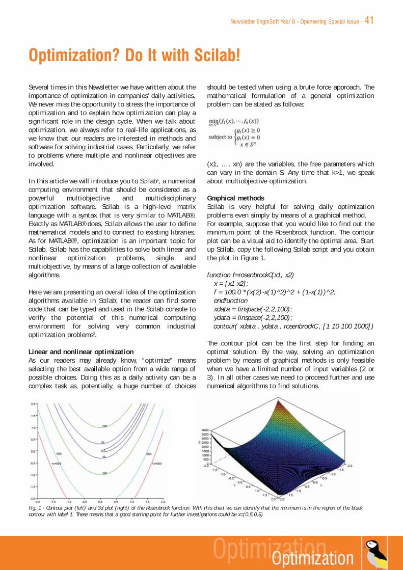
Newsletter EnginSoft Year 8 - Openeering Special Issue - 41
Several times in this Newsletter we have written about theimportance of optimization in companies’ daily activities.We never miss the opportunity to stress the importance ofoptimization and to explain how optimization can play asignificant role in the design cycle. When we talk aboutoptimization, we always refer to real-life applications, aswe know that our readers are interested in methods andsoftware for solving industrial cases. Particularly, we referto problems where multiple and nonlinear objectives areinvolved.
In this article we will introduce you to Scilab1, a numericalcomputing environment that should be considered as apowerful multiobjective and multidisciplinaryoptimization software. Scilab is a high-level matrixlanguage with a syntax that is very similar to MATLAB®.Exactly as MATLAB® does, Scilab allows the user to definemathematical models and to connect to existing libraries.As for MATLAB®2, optimization is an important topic forScilab. Scilab has the capabilities to solve both linear andnonlinear optimization problems, single andmultiobjective, by means of a large collection of availablealgorithms.
Here we are presenting an overall idea of the optimizationalgorithms available in Scilab; the reader can find somecode that can be typed and used in the Scilab console toverify the potential of this numerical computingenvironment for solving very common industrialoptimization problems3.
Linear and nonlinear optimizationAs our readers may already know, “optimize” meansselecting the best available option from a wide range ofpossible choices. Doing this as a daily activity can be acomplex task as, potentially, a huge number of choices
should be tested when using a brute force approach. Themathematical formulation of a general optimizationproblem can be stated as follows:
(x1, …, xn) are the variables, the free parameters whichcan vary in the domain S. Any time that k>1, we speakabout multiobjective optimization.
Graphical methodsScilab is very helpful for solving daily optimizationproblems even simply by means of a graphical method.For example, suppose that you would like to find out theminimum point of the Rosenbrock function. The contourplot can be a visual aid to identify the optimal area. Startup Scilab, copy the following Scilab script and you obtainthe plot in Figure 1.
function f=rosenbrockC(x1, x2)x = [x1 x2];f = 100.0 *(x(2)-x(1)^2)^2 + (1-x(1))^2;endfunctionxdata = linspace(-2,2,100); ydata = linspace(-2,2,100);contour( xdata , ydata , rosenbrockC , [1 10 100 1000])
The contour plot can be the first step for finding anoptimal solution. By the way, solving an optimizationproblem by means of graphical methods is only feasiblewhen we have a limited number of input variables (2 or3). In all other cases we need to proceed further and usenumerical algorithms to find solutions.
Fig. 1 - Contour plot (left) and 3d plot (right) of the Rosenbrock function. With this chart we can identify that the minimum is in the region of the blackcontour with label 1. These means that a good starting point for further investigations could be x=(0.5,0.5)
Optimization? Do It with Scilab!

Optimization algorithmsA large collection of different numerical methods isavailable for further investigations. There are tens ofoptimization algorithms in Scilab, and each method canbe used to solve a specific problem according to thenumber and smoothness of functions f, the number andtype of variables x, the number and type of constraints g.Some methods can be more suitable for constrainedoptimization, others may be better for convex problems,others can be tailored for solving discrete problems.Specific methods can be useful for solving quadraticprogramming, nonlinear problems, nonlinear least squares,nonlinear equations, multiobjective optimization, andbinary integer programming. Table 1 gives an overview ofthe optimization algorithms available in Scilab. Manyother optimization methods are made available from thecommunity every day as external modules using the ATOMSPortal, http://atoms.scilab.org/.
For showing the potentiality of Scilab as an optimizationtool, we can start from the most used optimization
function: optim. This command provides a set ofalgorithms for nonlinear unconstrained and bound-constrained optimization problems.Let’s see what happens if we use the optim function forthe previous problem:
function [ f , g, ind ] = rosenbrock ( x , ind )f = 100*(x(2)-x(1)^2)^2+(1-x(1))^2;g(1) = - 400. * ( x(2) - x(1)^2 ) * x(1) -2. * ( 1. - x(1) )g(2) = 200. * ( x(2) - x(1)^2 )
endfunctionx0 = [-1.2 1];[f, x] = optim(rosenbrock, x0);// Display results4
mprintf("x = %s\n", strcat(string(x)," "));mprintf("f = %e\n", f);
If we use x0=[-1.2 1] as initial point, the functionconverges easily to the optimal point x*=[1,1] with f=0.0.The previous example calculates both the value of theRosenbrock function and its gradient, as the gradient isrequired by the optimization method. In many real caseapplications, the gradient can be too complicated to becomputed or simply not available since the function is notknown and available only as a black-box from an externalfunction calculation. For this reason, Scilab has the abilityto compute the gradient using finite differences by meansof the function derivative or the function numdiff.
For example the following code define a function f andcompute the gradient on a specific point x.
function f=myfun(x)f=x(1)*x(1)+x(1)*x(2)
endfunctionx=[5 8]g=numdiff(myfun,x)
These two functions (derivative and numdiff) can be usedtogether with optim to minimize problem where gradient
is too complicated to be programmed. The optim function uses a quasi-Newtonmethod based on BFGS formula that is anaccurate algorithm for local optimization.On the same example, we can even applya different optimization approach such asthe derivative-free Nelder-Mead Simplex[1] that is implemented in the functionfminsearch. To do that we just have tosubstitute the line:
[f, x] = optim(rosenbrock, x0);With[x,f] = fminsearch(rosenbrock, x0);
This Nelder-Mead Simplex algorithm,starting from the same initial point,
Fig. 2 - Convergence of the Nelder-Mead Simplex algorithms (fminsearchfunction) on the Rosenbrock example.
Table 1 - This table gives an overview of the optimization algorithms available in Scilab and the typeof optimization problems which can be solved. For the constraints columns, the letter “l” means“linear”. For the problem size s,m,l indicate small, medium and large respectively that means lessthan ten, tens or hundreds of variables
42 - Newsletter EnginSoft Year 8 - Openeering Special Issue

converges very closely to the optimal point and preciselyto x*=[1.000022 1.0000422] with f=8.177661e-010. Thisshows that the second approach is less accurate than theprevious one: this is the price to pay in order to have amore robust approach that is less influenced by noisyfunctions and local optima.Figure 2 shows the convergence of the Nelder-MeadSimplex method on the Rosenbrock function.
It is important to say that, in the previous example, thefunction is given by means of a Scilab script but this wasonly done for simplicity. It is always possible to evaluatethe function f as an external function such as a C, Fortranor Java program or external commercial solver.
Parameter identification using measured data In this short paragraph we show a specific optimizationproblem that is very common in engineering. Wedemonstrate how fast and easy it can be to make aparametric identification for nonlinear systems, based oninput/output data.
Suppose for example that we have a certain number ofmeasurements in the matrix X and the value of the outputin the vector Y. Suppose that we know the functiondescribing the model (FF) apart from a set of parametersp and we would like to find out the value of thoseparameters. It is sufficient to write few lines of Scilabcode to solve the problem:
//model with parameters pfunction y=FF(x, p)
y=p(1)*(x-p(2))+p(3)*x.*x;endfunction
Z=[Y;X];//The criterion for evaluating the errorfunction e=G(p, z)
y=z(1),x=z(2);e=y-FF(x,p),
endfunction
//Solve the problem giving an initial guess for pp0=[1;2;3] [p,err]=datafit(G,Z,p0);
This method is very fast and efficient, it can findparameters for a high number of input/output data.Moreover it can take into consideration parameters’bounds and weights for points.
Evolutionary Algorithms: Genetic and MultiobjectiveGenetic algorithms [2] are search methods based on themechanics of natural evolution and selection. Thesemethods are widely used for solving highly non-linearreal-life problems because of their ability to remain robusteven against noisy functions and local optima. Genetic
algorithms are largely used in real-world problems as wellas in a number of engineering applications that are hardto solve with “classical” methods.
Using the genetic algorithms in Scilab is very simple: in afew lines it is possible to set the required parameters suchas the number of generations, the population size, theprobability of cross-over and mutation. Fig. 3 shows asingle objective genetic algorithm optim_ga on theRosenbrock function. Twenty initial random points (inyellow) evolve through 50 generations towards theoptimal point. The final generation is plotted in red.
MultiobjectiveScilab is not only for single objective problems. It caneasily deal with multiobjective optimization problems.Just to list one of the available methods, Scilab users cantake advantage of the NSGA-II. NSGA-II is the secondversion of the famous “Non-dominated Sorting GeneticAlgorithm” based on the work of Prof. Kalyanmoy Deb [3].
Fig. 3 - Optimization of the Rosenbrock function by means of a GeneticAlgorithm. Initial random population is in yellow, final population is in redand converges to the real optimal solution.
Fig. 4 - ZDT1 problem solved with the Scilab’s NSGA-II optimizationalgorithm. Red points on the top represents the initial populations, blackpoints on the bottom the final Pareto population. The solid line representsthe Pareto frontier that, in this specific example, is a continuous convexsolution.
Newsletter EnginSoft Year 8 - Openeering Special Issue - 43
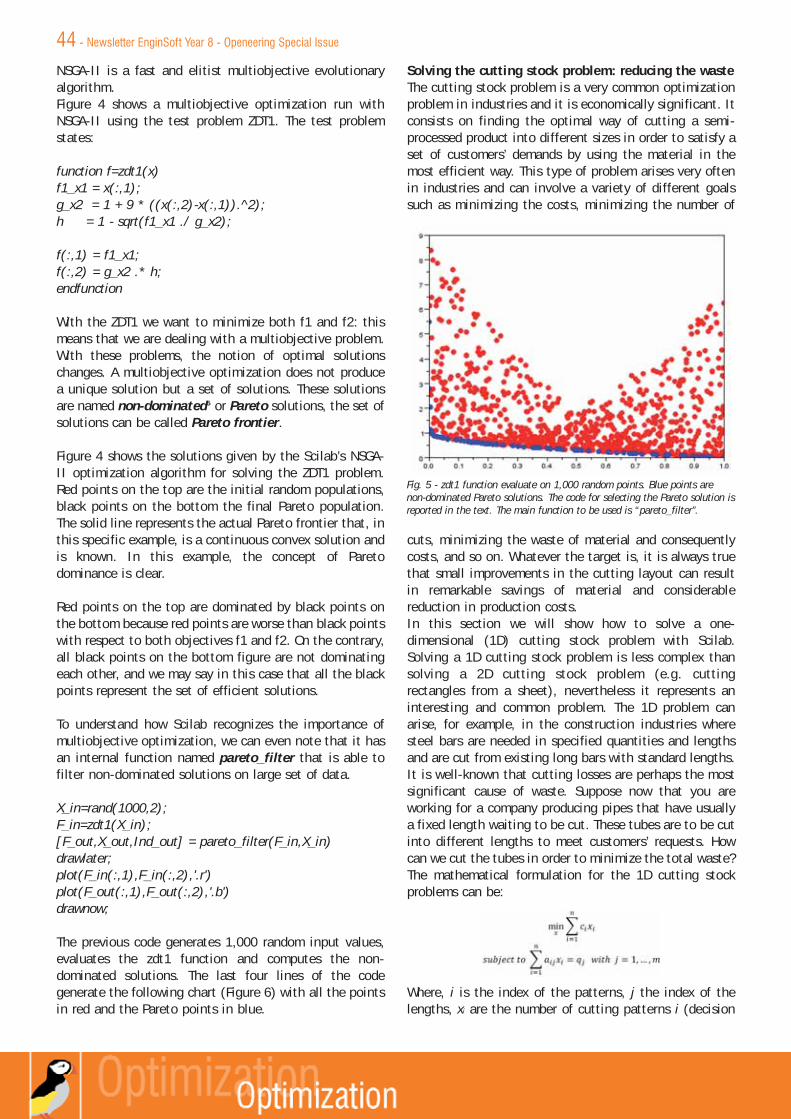
NSGA-II is a fast and elitist multiobjective evolutionaryalgorithm.Figure 4 shows a multiobjective optimization run withNSGA-II using the test problem ZDT1. The test problemstates:
function f=zdt1(x)f1_x1 = x(:,1);g_x2 = 1 + 9 * ((x(:,2)-x(:,1)).^2);h = 1 - sqrt(f1_x1 ./ g_x2);
f(:,1) = f1_x1;f(:,2) = g_x2 .* h;endfunction
With the ZDT1 we want to minimize both f1 and f2: thismeans that we are dealing with a multiobjective problem.With these problems, the notion of optimal solutionschanges. A multiobjective optimization does not producea unique solution but a set of solutions. These solutionsare named non-dominated5 or Pareto solutions, the set ofsolutions can be called Pareto frontier.
Figure 4 shows the solutions given by the Scilab’s NSGA-II optimization algorithm for solving the ZDT1 problem.Red points on the top are the initial random populations,black points on the bottom the final Pareto population.The solid line represents the actual Pareto frontier that, inthis specific example, is a continuous convex solution andis known. In this example, the concept of Paretodominance is clear.
Red points on the top are dominated by black points onthe bottom because red points are worse than black pointswith respect to both objectives f1 and f2. On the contrary,all black points on the bottom figure are not dominatingeach other, and we may say in this case that all the blackpoints represent the set of efficient solutions.
To understand how Scilab recognizes the importance ofmultiobjective optimization, we can even note that it hasan internal function named pareto_filter that is able tofilter non-dominated solutions on large set of data.
X_in=rand(1000,2);F_in=zdt1(X_in);[F_out,X_out,Ind_out] = pareto_filter(F_in,X_in)drawlater;plot(F_in(:,1),F_in(:,2),'.r')plot(F_out(:,1),F_out(:,2),'.b')drawnow;
The previous code generates 1,000 random input values,evaluates the zdt1 function and computes the non-dominated solutions. The last four lines of the codegenerate the following chart (Figure 6) with all the pointsin red and the Pareto points in blue.
Solving the cutting stock problem: reducing the wasteThe cutting stock problem is a very common optimizationproblem in industries and it is economically significant. Itconsists on finding the optimal way of cutting a semi-processed product into different sizes in order to satisfy aset of customers’ demands by using the material in themost efficient way. This type of problem arises very oftenin industries and can involve a variety of different goalssuch as minimizing the costs, minimizing the number of
cuts, minimizing the waste of material and consequentlycosts, and so on. Whatever the target is, it is always truethat small improvements in the cutting layout can resultin remarkable savings of material and considerablereduction in production costs.In this section we will show how to solve a one-dimensional (1D) cutting stock problem with Scilab.Solving a 1D cutting stock problem is less complex thansolving a 2D cutting stock problem (e.g. cuttingrectangles from a sheet), nevertheless it represents aninteresting and common problem. The 1D problem canarise, for example, in the construction industries wheresteel bars are needed in specified quantities and lengthsand are cut from existing long bars with standard lengths.It is well-known that cutting losses are perhaps the mostsignificant cause of waste. Suppose now that you areworking for a company producing pipes that have usuallya fixed length waiting to be cut. These tubes are to be cutinto different lengths to meet customers’ requests. Howcan we cut the tubes in order to minimize the total waste?The mathematical formulation for the 1D cutting stockproblems can be:
Where, i is the index of the patterns, j the index of thelengths, xi are the number of cutting patterns i (decision
Fig. 5 - zdt1 function evaluate on 1,000 random points. Blue points arenon-dominated Pareto solutions. The code for selecting the Pareto solution isreported in the text. The main function to be used is “pareto_filter”.
44 - Newsletter EnginSoft Year 8 - Openeering Special Issue

variables) and ci are the costs of the pattern i. A=(aij) thematrix of all possible patterns and qj the customers’requests. We may say that the value aij indicates thenumber of pieces of length j within one pipe cut in thepattern i. The goal of this model is to minimize theobjective function which consists of the total costs of thecutting phase. If ci is equal to 1 for all the patterns, thegoal corresponds to the total number of pipes required toaccomplish the requirements.
Let’s make a practical example and solve it with Scilab.Suppose that we have 3 possible sizes, 55mm, 26mm, and24mm in which we can cut the original pipe of 100 mm.The possible patterns are:1. One cut of type one and one of type two and zero of
type three [1 1 0]2. One cut of type one and one of type three [1 0 1]3. Two cut of type two and two of type three [0 2 2]
These patterns define the matrix A. Then we have thecosts that are 4, 3 and 1 for the pattern 1, 2 and 3respectively. The total request from the customers are:150 pieces of length 55mm, 200 with length equal to26mm and 300 pieces with length 24mm.For solving this problem in Scilab we can use this script.
//patternaij=[ 1 1 0;
1 0 1;0 2 2];
//costs ci=[4; 3; 1];//requestqj=[150; 200; 300];
xopt = karmarkar(aij',qj,ci)
Running this script with Scilab you obtain xopt=[25, 125,87.5], this means that to satisfy the requests reducing thetotal number of pipes we have to cut 25 times the pattern(1), 125 times with pattern (2) and 87.5 times the pattern(3).We show here a simple case with only three differentrequests and three different patterns. The problem can bemuch more complicated, with many more options, manydifferent dimensions, costs and requests. It may includethe maximum number of cuts on a single piece, it mayrequire a bit of effort in generating the list of feasiblepatterns (i.e. the matrix A). All these difficulties can becoded with Scilab and the logic behind the approachremains the same.The previous script uses the Karmarkar’s algorithm [4] tosolve this linear problem. The result gives an output thatis not an integer solution, hence we need to approximatebecause we cannot cut 87.5 pipes with the third pattern.This approximated solution can be improved with anotherdifferent optimization algorithm, for example evaluating
the nearest integer solutions or using a more robustgenetic algorithm. But even if we stop with the first stepand we round off the solution, we have a good reductionof waste.
ConclusionsAs the solution of the cutting stock problemdemonstrates, Scilab is not just an educational tool but aproduct for solving real industrial problems. The cuttingstock problem is a common issue in industries, and a goodsolution can result in remarkable savings. By the way, inthis article we presented only a small subset of thepossibilities that a Scilab user can have for solving real-world problems. For the sake of simplicity, this paper shows only verytrivial functions that have been used for the purpose ofmaking a short and general tutorial. Obviously thesesimple functions can be substituted by more complex andtime consuming ones such as FEM solvers or other externalsimulation codes.MATLAB® users have probably recognized the similaritiesbetween the commercial software and Scilab. We hope allother readers have not been scared by the fact thatproblems and methods should be written down as scripts.Once the logic is clear, writing down scripts can result inan agile and exciting activity.
For more information and for the original version of Scilabscripts:Silvia Poles – [email protected]
References[1]Nelder, John A.; R. Mead (1965). "A simplex method
for function minimization". Computer Journal 7:308–313
[2]David E. Goldberg. Genetic Algorithms in Search,Optimization & Machine Learning. Addison-Wesley,1989.
[3]N. Srinivas and Kalyanmoy Deb. Multiobjectiveoptimization using nondominated sorting in geneticalgorithms. Evolutionary Computation, 2:221{248,1994
[4]Narendra Karmarkar (1984). "A New Polynomial TimeAlgorithm for Linear Programming", Combinatorica, Vol4, nr. 4, p. 373–395.
1 Download Scilab for free at http://www.scilab.org/2 MATLAB is a registered trademark of The MathWorks, Inc3 Contact the author for the original version of the Scilab
scripts4 The symbol “//” indicates a comment5 By definition we say that the design a dominates b if [f1(a)
<= f1(b) and f2(a) <= f2(b)...and fk(a) <= fk(b)], for all thef and [f1(a) < f1(b) or f2(a) < f2(b)...or fk(a) < fk(b)] for atleast one f
Newsletter EnginSoft Year 8 - Openeering Special Issue - 45
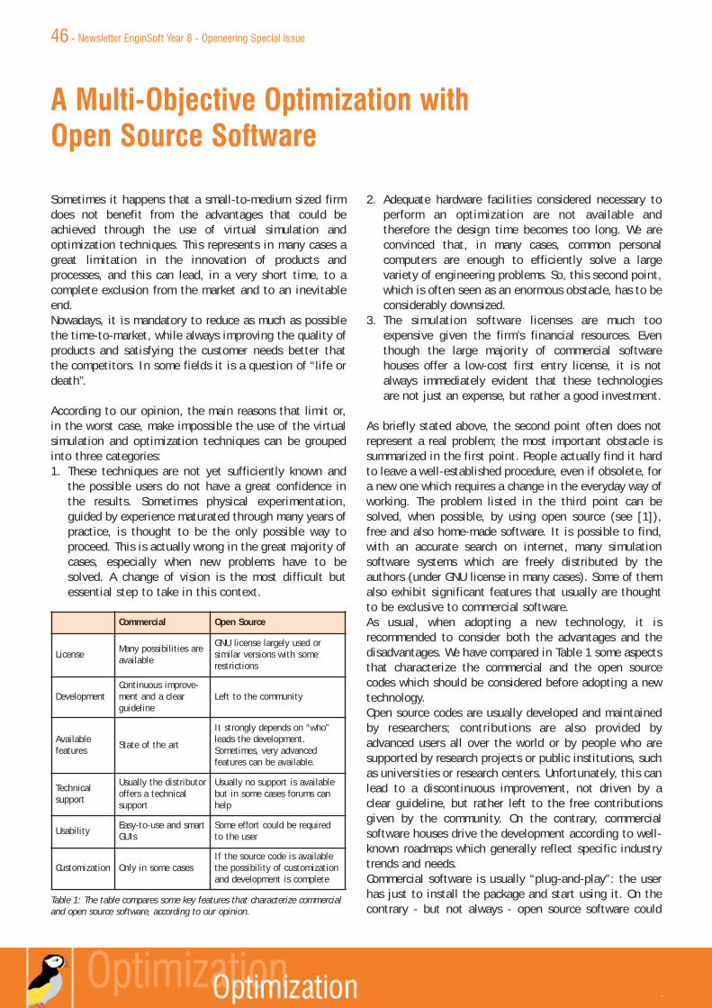
Sometimes it happens that a small-to-medium sized firmdoes not benefit from the advantages that could beachieved through the use of virtual simulation andoptimization techniques. This represents in many cases agreat limitation in the innovation of products andprocesses, and this can lead, in a very short time, to acomplete exclusion from the market and to an inevitableend.Nowadays, it is mandatory to reduce as much as possiblethe time-to-market, while always improving the quality ofproducts and satisfying the customer needs better thatthe competitors. In some fields it is a question of “life ordeath”.
According to our opinion, the main reasons that limit or,in the worst case, make impossible the use of the virtualsimulation and optimization techniques can be groupedinto three categories:1. These techniques are not yet sufficiently known and
the possible users do not have a great confidence inthe results. Sometimes physical experimentation,guided by experience maturated through many years ofpractice, is thought to be the only possible way toproceed. This is actually wrong in the great majority ofcases, especially when new problems have to besolved. A change of vision is the most difficult butessential step to take in this context.
2. Adequate hardware facilities considered necessary toperform an optimization are not available andtherefore the design time becomes too long. We areconvinced that, in many cases, common personalcomputers are enough to efficiently solve a largevariety of engineering problems. So, this second point,which is often seen as an enormous obstacle, has to beconsiderably downsized.
3. The simulation software licenses are much tooexpensive given the firm’s financial resources. Eventhough the large majority of commercial softwarehouses offer a low-cost first entry license, it is notalways immediately evident that these technologiesare not just an expense, but rather a good investment.
As briefly stated above, the second point often does notrepresent a real problem; the most important obstacle issummarized in the first point. People actually find it hardto leave a well-established procedure, even if obsolete, fora new one which requires a change in the everyday way ofworking. The problem listed in the third point can besolved, when possible, by using open source (see [1]),free and also home-made software. It is possible to find,with an accurate search on internet, many simulationsoftware systems which are freely distributed by theauthors (under GNU license in many cases). Some of themalso exhibit significant features that usually are thoughtto be exclusive to commercial software.As usual, when adopting a new technology, it isrecommended to consider both the advantages and thedisadvantages. We have compared in Table 1 some aspectsthat characterize the commercial and the open sourcecodes which should be considered before adopting a newtechnology.Open source codes are usually developed and maintainedby researchers; contributions are also provided byadvanced users all over the world or by people who aresupported by research projects or public institutions, suchas universities or research centers. Unfortunately, this canlead to a discontinuous improvement, not driven by aclear guideline, but rather left to the free contributionsgiven by the community. On the contrary, commercialsoftware houses drive the development according to well-known roadmaps which generally reflect specific industrytrends and needs.Commercial software is usually “plug-and-play”: the userhas just to install the package and start using it. On thecontrary - but not always - open source software could
A Multi-Objective Optimization with Open Source Software
Commercial Open Source
LicenseMany possibilities are available
GNU license largely used orsimilar versions with somerestrictions
DevelopmentContinuous improve-ment and a clear guideline
Left to the community
Available features
State of the art
It strongly depends on “who”leads the development.Sometimes, very advanced features can be available.
Technicalsupport
Usually the distributoroffers a technicalsupport
Usually no support is availablebut in some cases forums canhelp
UsabilityEasy-to-use and smartGUIs
Some effort could be requiredto the user
Customization Only in some casesIf the source code is availablethe possibility of customizationand development is complete
Table 1: The table compares some key features that characterize commercialand open source software, according to our opinion.
46 - Newsletter EnginSoft Year 8 - Openeering Special Issue
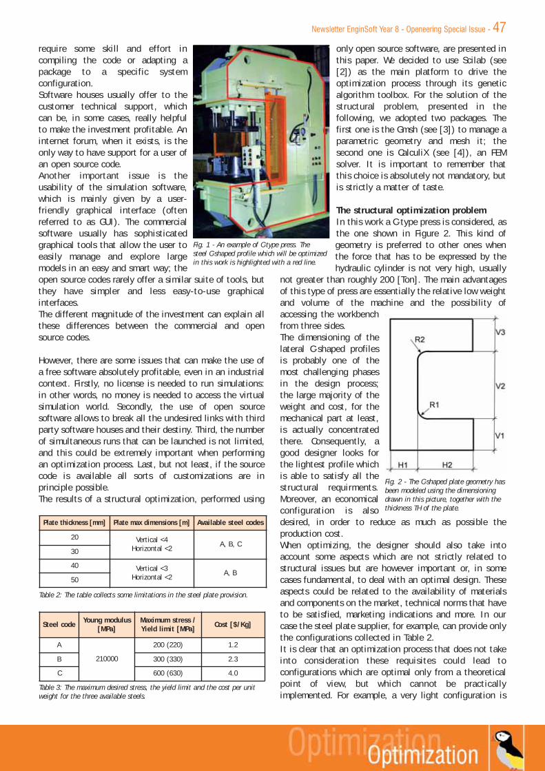
require some skill and effort incompiling the code or adapting apackage to a specific systemconfiguration.Software houses usually offer to thecustomer technical support, whichcan be, in some cases, really helpfulto make the investment profitable. Aninternet forum, when it exists, is theonly way to have support for a user ofan open source code.Another important issue is theusability of the simulation software,which is mainly given by a user-friendly graphical interface (oftenreferred to as GUI). The commercialsoftware usually has sophisticatedgraphical tools that allow the user toeasily manage and explore largemodels in an easy and smart way; theopen source codes rarely offer a similar suite of tools, butthey have simpler and less easy-to-use graphicalinterfaces.The different magnitude of the investment can explain allthese differences between the commercial and opensource codes.
However, there are some issues that can make the use ofa free software absolutely profitable, even in an industrialcontext. Firstly, no license is needed to run simulations:in other words, no money is needed to access the virtualsimulation world. Secondly, the use of open sourcesoftware allows to break all the undesired links with thirdparty software houses and their destiny. Third, the numberof simultaneous runs that can be launched is not limited,and this could be extremely important when performingan optimization process. Last, but not least, if the sourcecode is available all sorts of customizations are inprinciple possible.The results of a structural optimization, performed using
only open source software, are presented inthis paper. We decided to use Scilab (see[2]) as the main platform to drive theoptimization process through its geneticalgorithm toolbox. For the solution of thestructural problem, presented in thefollowing, we adopted two packages. Thefirst one is the Gmsh (see [3]) to manage aparametric geometry and mesh it; thesecond one is CalculiX (see [4]), an FEMsolver. It is important to remember thatthis choice is absolutely not mandatory, butis strictly a matter of taste.
The structural optimization problemIn this work a C-type press is considered, asthe one shown in Figure 2. This kind ofgeometry is preferred to other ones whenthe force that has to be expressed by thehydraulic cylinder is not very high, usually
not greater than roughly 200 [Ton]. The main advantagesof this type of press are essentially the relative low weightand volume of the machine and the possibility ofaccessing the workbenchfrom three sides.The dimensioning of thelateral C-shaped profilesis probably one of themost challenging phasesin the design process;the large majority of theweight and cost, for themechanical part at least,is actually concentratedthere. Consequently, agood designer looks forthe lightest profile whichis able to satisfy all thestructural requirments.Moreover, an economicalconfiguration is alsodesired, in order to reduce as much as possible theproduction cost.When optimizing, the designer should also take intoaccount some aspects which are not strictly related tostructural issues but are however important or, in somecases fundamental, to deal with an optimal design. Theseaspects could be related to the availability of materialsand components on the market, technical norms that haveto be satisfied, marketing indications and more. In ourcase the steel plate supplier, for example, can provide onlythe configurations collected in Table 2.It is clear that an optimization process that does not takeinto consideration these requisites could lead toconfigurations which are optimal only from a theoreticalpoint of view, but which cannot be practicallyimplemented. For example, a very light configuration is
Fig. 1 - An example of C-type press. The steel C-shaped profile which will be optimizedin this work is highlighted with a red line.
Plate thickness [mm] Plate max dimensions [m] Available steel codes
20 Vertical <4Horizontal <2
A, B, C30
40 Vertical <3Horizontal <2
A, B50
Table 2: The table collects some limitations in the steel plate provision.
Steel code Young modulus[MPa]
Maximum stress / Yield limit [MPa] Cost [$/Kg]
A
210000
200 (220) 1.2
B 300 (330) 2.3
C 600 (630) 4.0
Table 3: The maximum desired stress, the yield limit and the cost per unitweight for the three available steels.
Fig. 2 - The C-shaped plate geometry hasbeen modeled using the dimensioningdrawn in this picture, together with thethickness TH of the plate.
Newsletter EnginSoft Year 8 - Openeering Special Issue - 47

not of practical interest, if it requires a steel characterizedby a yield limit greater that 600 [MPa].For this reason all the requirements collected in Tables 2and 3 have been included in order to drive theoptimization algorithm to feasible and interestingsolutions.
Moreover, it is required that the hollow in the plate (H2-max(R1,R2) x V2, see Figure 2) is at least 500 x 500 [mm]to allow the positioning of the transversal plates and thehydraulic cylinder.
Another technical requisite is that the maximum verticaldisplacement is less than 5 [mm] to avoid excessivemisalignments between the cylinder axis and the structureunder the usual operating conditions. This limit has beenchosen arbitrarily, in the attempt to exclude the designsthat are not sufficiently stiff, taking into account,however, that the C-plate is a part of a more complex realstructure which will be much more stiff than what iscalculated with this simple model.A designer should recognize that the solution of such aproblem is not exactly trivial. Firstly, it is not easy to finda configuration which is able to satisfy all the requisiteslisted above; secondly, it is rather challenging to obtain adesign that minimizes both the volume of the plate (theweight) and the production cost.
The open source software for the structural analysisGmsh has been used as a preprocessor to managethe parametric geometry of the C-shaped plate andmesh it in batch mode. Gmsh has the ability to mesha non-regular geometry using triangular elements;many controls are available to efficiently define thetypical element dimension, the refinement depthand more. It is a very powerful software tool whichis also able to manage complicated three-dimensional geometries and efficiently mesh themusing a rich element library.The mesh can be exported in a formatted text filewhere the nodes and the element connectivities arelisted together with some useful information relatedto the so-called physical entities, previously defined
by the user; this information can be used to correctlyapply, for example, boundary conditions, domainproperties and loads to a future finite element model.The CalculiX finite element software has been used tosolve the linear elastic problem. Also in this case a batchrun is available; among the many interesting features thatthis software offers are the easy input text format, and theability to perform both linear and non-linear static anddynamic analyses.CalculiX also offers a pre and post processingenvironment, called CalculiX GraphiX, which can be usedto prepare quite complicated models and, above all,display results.These two software tools are both well documented andalso some useful examples are provided for new users. Theinput and output formats are, in both cases, easy tounderstand and manage.In order to make the use of these tools completelyautomatic, it is necessary to write a procedure thattranslates the mesh output file produced by Gmsh into aninput file readable by CalculiX. This translation is arelatively simple operation and it can be performedwithout a great effort using a variety of programminglanguages; a text file has to be read, some informationhas to be captured and then rewritten into a text fileusing some simple rules. For this, a simple executable file(named translate.exe) has been compiled and it will belaunched whenever necessary.A similar operation has also to be performed in anoptimization context to extract the interesting quantitiesfrom the CalculiX result file and rewrite them into acompact and accessible text file.As before, an executable file (named read.exe) has beenproduced to read the .dat results file and write thevolume, the maximum vertical displacement and the nodalvon Mises stress corresponding to a given design into afile named results.out.Many other open source software codes are available, bothfor the model setup and for its solution. Also for theresults visualization, there are many free tools withpowerful features. For this reason the interested reader
Fig. 3 - A possible version of the C-shaped plate meshed in Gmsh.
Fig. 4 - The CalculiX GraphiX window, where the von Mises stress for the C-shaped plate is plotted.
48 - Newsletter EnginSoft Year 8 - Openeering Special Issue

can imagine the use of other toolsto solve this problem in anefficient way.
The optimization process drivenby Scilab The genetic algorithm toolbox, byYan Collette, is available in thestandard installation of Scilab andit can be used to solve the multi-objective optimization problemdescribed above. This toolbox iscomposed of some routines whichimplement both a MOGA and a
NSGA2 algorithm and also a version for the operationsthat have been performed when running a geneticalgorithm, that is the encoding, the crossover, the
mutation and the selection.These routines are extremely flexibleand they can be modified by the useraccording to his or her own needs,since the source code is available. Thisis exactly what we have done,modifying the optim_moga.sci script tohandle the constraints (with a penaltyapproach) and manage the infeasibledesigns efficiently (i.e.: all theconfigurations which cannot becomputed); we have then redefined thecoding_ga_binary.sci to allow thediscretization of the input variables as
listed in Table 4. Othersmall changes have beenmade to the routines toperform some marginaloperations, such aswriting partial results to afile.When the geneticalgorithm requires the
evaluation of a given configuration, we run a Scilab scriptwhich is charged to prepare all the text files needed toperform the run and then launch the software (Gmsh,
CalculiX and the otherexecutables) through a call tothe system in the right order.The script finally loads theresults needed by theoptimization.It is important to highlightthat this script can be easilychanged to launch othersoftware tools or perform otheroperations whenever necessary.In our case, eight inputvariables are sufficient tocompletely parameterize thegeometry of the plate (seeFigure 2): the lower and upperbounds together with the stepsare collected in Table 4. Notethat the lower bound ofvariable V2 has been set to 500[mm], in order to satisfy theconstraint on the minimalvertical dimension required forthe hollow.We can use a rich initialpopulation, (200 designsrandomly generated),considering the fact that a highnumber of them will violate theimposed constraints, or worse,be unfeasible. The following
VariableLowerbound[mm]
Upperbound[mm]
Step[mm]
H1 250 150. 5
H2 500 1500 5
V1 250 1500 5
V2 500 1500 5
V3 250 1500 5
R1 50 225 5
R2 50 225 5
TH 20 50 10
Table 4: The lower and upper bounds together with thestep for the input variables.
Designname
H1[mm]
H2[mm]
V1[mm]
V2[mm]
V3[mm]
R1[mm]
R2[mm]
TH[mm]
Cost[$]
maxvM
stress [MPa]
max vertical displ.[mm]
Volume[mm3]
A 670 665 575 500 490 165 110 20 1304 577.7 4.93 3.53.107
B 1155 695 725 545 840 185 165 30 1097 199.8 1.73 1.06.108
Table 5: The optimal solutions.
Fig. 5 - The Cost of the computed configurations can be plotted versus the Volume. Red points stand for the feasi-ble configurations while the blue plus indicates the configurations that do not respect one constraint at least. The two green squares are the Pareto (optimal) solutions (A and B in Table 5).
Fig. 6 - The vertical displacement for the design A. Fig.7 - The von Mises stress for the design A.
Newsletter EnginSoft Year 8 - Openeering Special Issue - 49

50 - Newsletter EnginSoft Year 8 - Openeering Special Issue
generations will howeverconsist of only 50 designs, tolimit the optimization time.After 50 generations we obtainthe results plotted in Figure 5and Table 5, where the twoPareto (optimal) solutions arecollected. We finally decided tochoose, between the twooptimal ones, the configurationwith the lowest volume (namedas “A” in Table 5).
In Figures 6 and 7 the verticaldisplacement and the von Misesstress are plotted for the optimal configuration named “A”(see Table 5). Note that during the optimization, themaximum value of the von Mises stress computed in thefinite element Gauss points has been used, while in Figure7 the von Mises stress extrapolated by CalculiX to themesh nodes is plotted; this is the reason why the
maximum values are different. However, they are both lessthan the yield limit corresponding to the steel type C, asreported in Table 3.Another interesting consideration is that the Pareto frontin our case consists of just two designs: this shows thatthe solution of this optimization problem is far fromtrivial.The design of the C-shaped plate can be further improved.If we run other generations with the optimizationalgorithm better solutions could probably be found, butwe feel that the improvements that might be obtained inthis way do not justify additional computations.Substantial improvements can be achieved in another way.Actually, if we look at the von Mises stress distributiondrawn in Figure 7 we note that the corners of the plate donot have a very high stress level and that they should notinfluence the structural behavior very much.A new design can be tested, cutting the corners of theplate; for the sake of simplicity we decided to use fourequal cuts of horizontal and vertical dimensions equal toH1/3, starting from the corners. The results are drawn inFigures 8 and 9, which can be compared with Figures 6and 7.As expected, there is a reduction in volume with respectto the original design, but no significant variations areregistered in the other outputs. This corroborates the idea
that the cut dimensions can be excluded from the set ofinput variables, since the output does not stronglydependent on them, and this leads to a simpleroptimization problem.The cost does not change; actually it represents the costof the rectangular plate needed to produce the C-shapedprofile.Other configurations with a lower volume can be probablyfound with some other runs; however, the reader has toconsider that these improvements are not reallysignificant in an industrial context, where, probably, it ismuch more important to find optimal solutions in a veryshort time.
ConclusionsIn this work it has been shown how it is possible to useopen source software to solve a non-trivial structuraloptimization problem.Some aspects which characterize the commercial and theopen source software have been stressed in order to helpthe reader to make his or her own best choice. We areconvinced that there is not a single right solution butrather that the best solution has to be found for eachsituation.Whichever the choice, the hope is that virtual simulationand optimization techniques are used to innovate.
References[1]Visit http://www.opensource.org/ to have more
information on open source software[2]Scilab can be freely downloaded from:
http://www.scilab.org/[3]Gmsh can be freely downloaded from:
http://www.geuz.org/gmsh/[4]Calculix can be freely downloaded from:
http://www.calculix.de/
ContactsFor more information on this document please contact theauthor:Massimiliano Margonari - [email protected]
Horizontal and verticallength of cuts starting
from corners [mm]
Cost[$]
max vMstress [MPa]
maxVerticaldispl.[mm]
Volume[mm3]
H1/3 1304 581.3 4.80 3.33.107
Table 6: The modified design. It can be seen that there is an interestingreduction in the volume with respect to the original design, the “A” configu-ration in Table 5. Other output quantities do not present significant varia-tions.
Fig. 8 - The vertical displacement for the modifieddesign.
Fig. 9 - The von Mises stress for the modified design.

Newsletter EnginSoft Year 8 - Openeering Special Issue - 51
Scilab training courses by Openeering
Openeering offers Scilab training courses designed withindustry in mind. Openeering trainers have the highestlevel of competence: not only they are skilled Scilabsoftware trainers, but, most importantly, they are seniorengineers and mathematicians with a deep knowledge inthe use of engineering and scientific software, knowinghow to apply Scilab to industry level case studies.
Openeering offers two sets of Scilab courses: scheduledstandard courses and tailored, custom courses. Standardcourses are provided on a regular basis, at differentlocations over Europe, aiming to provide a standardeducation trail, at introductory and specialized levels.Great care have been put in designing course syllabus andtraining materials. The Openeering training coursescalendar is continuously updated and is available on theopeneering.com website.
Openeering custom courses are tailored taking intoaccount the initial competencies of the trainees and thespecific customer needs. Custom courses can be providedat EnginSoft or at customer’s premises.
Country Location Date Date
Italy
TrentoMarch 20 and 21, 2012 SCILAB-01-IT - Introduzione a Scilab
March 22, 2012 SCILAB-02-IT - Ottimizzare con Scilab
BergamoJune 12 and 13, 2012 SCILAB-01-IT - Introduzione a Scilab
June 14, 2012 SCILAB-02-IT - Ottimizzare con Scilab
PadovaSeptember 11 and 12, 2012 SCILAB-01-IT - Introduzione a Scilab
September 13, 2012 SCILAB-02-IT - Ottimizzare con Scilab
GermanyFrankfurt amMain
October 3 and 4, 2012 SCILAB-01-EN – Introduction to Scilab
October 5, 2012 SCILAB-02-EN - Optimizing with Scilab
SCILAB-01: Introduction to ScilabThe course has two main objectives. At the end of thecourse, the trainee will be able to effectively useScilab. The trainee will also be aware of potentialScilab application and strategies to solve variouscommon industry problems, such as the cutting stockproblem, data fitting, Monte Carlo analysis, Six Sigma.
SCILAB-02: Optimizing with ScilabAt the end of the course the trainee will be able toapply Scilab to common optimization problems. Thecourse will provide the theoretical basis, such as howto correctly analyze and model single- and multi-objective optimization problems, and strategies tobuild real world optimization applications with Scilab.Participation to SCILAB-01 is strongly suggested.


![Newsletter - EnginSoft · shape with optimization ... Design exploration and optimization ... [ICEM CFD is a trademark used by ANSYS, Inc. under license]](https://img.dokumen.tips/doc/110x75/5b0785b97f8b9abf568e9cdd/newsletter-with-optimization-design-exploration-and-optimization-icem.jpg)