Embed Size (px)
Citation preview
3
Basic Tutorial
Overview of the Basic Tutorial . . . . . . . . . . . 3-2
Running a Simulation on the Host PC . . . . . . . . 3-3Running a Simulation of Your Model . . . . . . . . . . 3-4
Creating a Target Application . . . . . . . . . . . . 3-6Booting the Target PC . . . . . . . . . . . . . . . . 3-6Entering the Simulation Parameters . . . . . . . . . . 3-7Building and Downloading the Target Application . . . . . 3-11Troubleshooting the Build Process . . . . . . . . . . . 3-12
Running the Target Application on the Target PC . . . 3-12Starting and Stopping the Target Application . . . . . . . 3-13
Signal Logging . . . . . . . . . . . . . . . . . . . 3-15Plotting Outputs and States . . . . . . . . . . . . . . 3-15Plotting Task Execution Time . . . . . . . . . . . . . 3-16
Signal Tracing with the Host Scope . . . . . . . . . 3-18Creating a Scope Object and Selecting Signals . . . . . . . 3-19Closing All Scope Windows . . . . . . . . . . . . . . . 3-25
Signal Tracing with the Target Scope . . . . . . . . 3-26Creating a Target Scope Object and Selecting Signals . . . . 3-26
Signal Tracing with xPC Target Functions . . . . . . 3-31Creating a Target Scope Object and Selecting Signals . . . . 3-31
Parameter Tuning Using Simulink External Mode . . . 3-34Setting Up Simulink in External Mode . . . . . . . . . . 3-35Changing Simulink Block Parameters . . . . . . . . . . 3-36
Parameter Tuning with xPC Target Commands . . . . 3-38Changing the Target Object Properties . . . . . . . . . . 3-38
3 Basic Tutorial
3-2
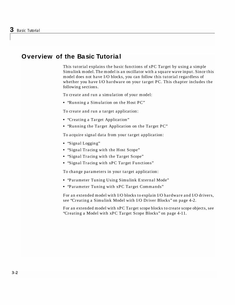
Overview of the Basic TutorialThis tutorial explains the basic functions of xPC Target by using a simpleSimulink model. The model is an oscillator with a square wave input. Since thismodel does not have I/O blocks, you can follow this tutorial regardless ofwhether you have I/O hardware on your target PC. This chapter includes thefollowing sections.
To create and run a simulation of your model:
• “Running a Simulation on the Host PC”
To create and run a target application:
• “Creating a Target Application”
• “Running the Target Application on the Target PC”
To acquire signal data from your target application:
• “Signal Logging”
• “Signal Tracing with the Host Scope”
• “Signal Tracing with the Target Scope”
• “Signal Tracing with xPC Target Functions”
To change parameters in your target application:
• “Parameter Tuning Using Simulink External Mode”
• “Parameter Tuning with xPC Target Commands”
For an extended model with I/O blocks to explain I/O hardware and I/O drivers,see “Creating a Simulink Model with I/O Driver Blocks” on page 4-2.
For an extended model with xPC Target scope blocks to create scope objects, see“Creating a Model with xPC Target Scope Blocks” on page 4-11.
Running a Simulation on the Host PC
3-3
Running a Simulation on the Host PCYou use Simulink in normal mode to observe the behavior of your model innonreal-time. This section includes the following topics:
• “Loading a Simulink Model”
• “Running a Simulation of Your Model”
For procedures to run your target application in real-time, see “Creating aTarget Application” on page 3-6.
Loading a Simulink ModelLoading a Simulink model moves information about your model, including theblock parameters, into the MATLAB workspace.
After you create and save a Simulink model, you can load it back into theMATLAB workspace. This procedure uses the Simulink model xpcosc.mdl asan example.
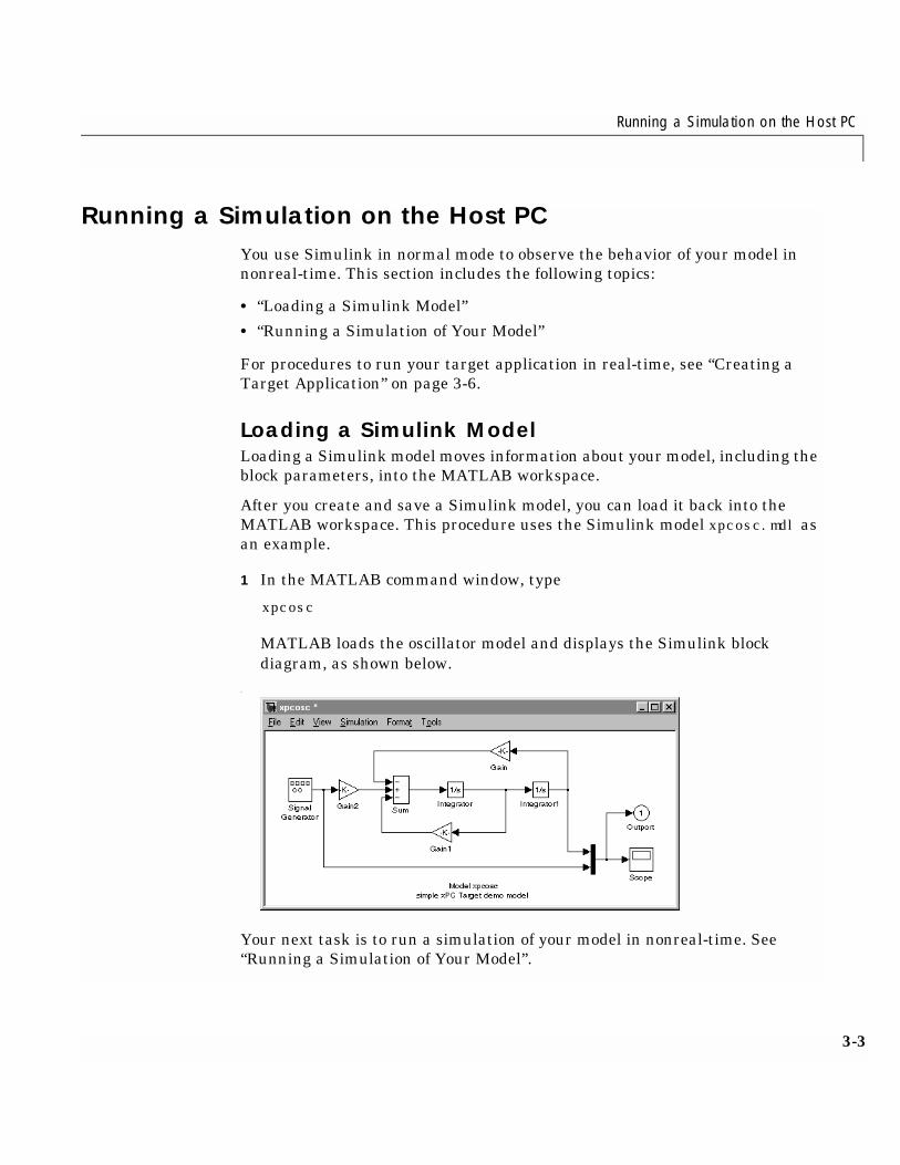
1 In the MATLAB command window, type
xpcosc
MATLAB loads the oscillator model and displays the Simulink blockdiagram, as shown below.
.
Your next task is to run a simulation of your model in nonreal-time. See“Running a Simulation of Your Model”.
3 Basic Tutorial
3-4
Running a Simulation of Your ModelYou run a simulation of your model in nonreal-time to observe the behavior ofyour model.
After you load your Simulink model into the MATLAB workspace, you can runa simulation. This procedure uses the Simulink model xpcosc.mdl as anexample and assumes you have already loaded that model.
Simulating the Model Using the Simulink Graphical User InterfaceTo simulate the oscillator model, use the following procedure.
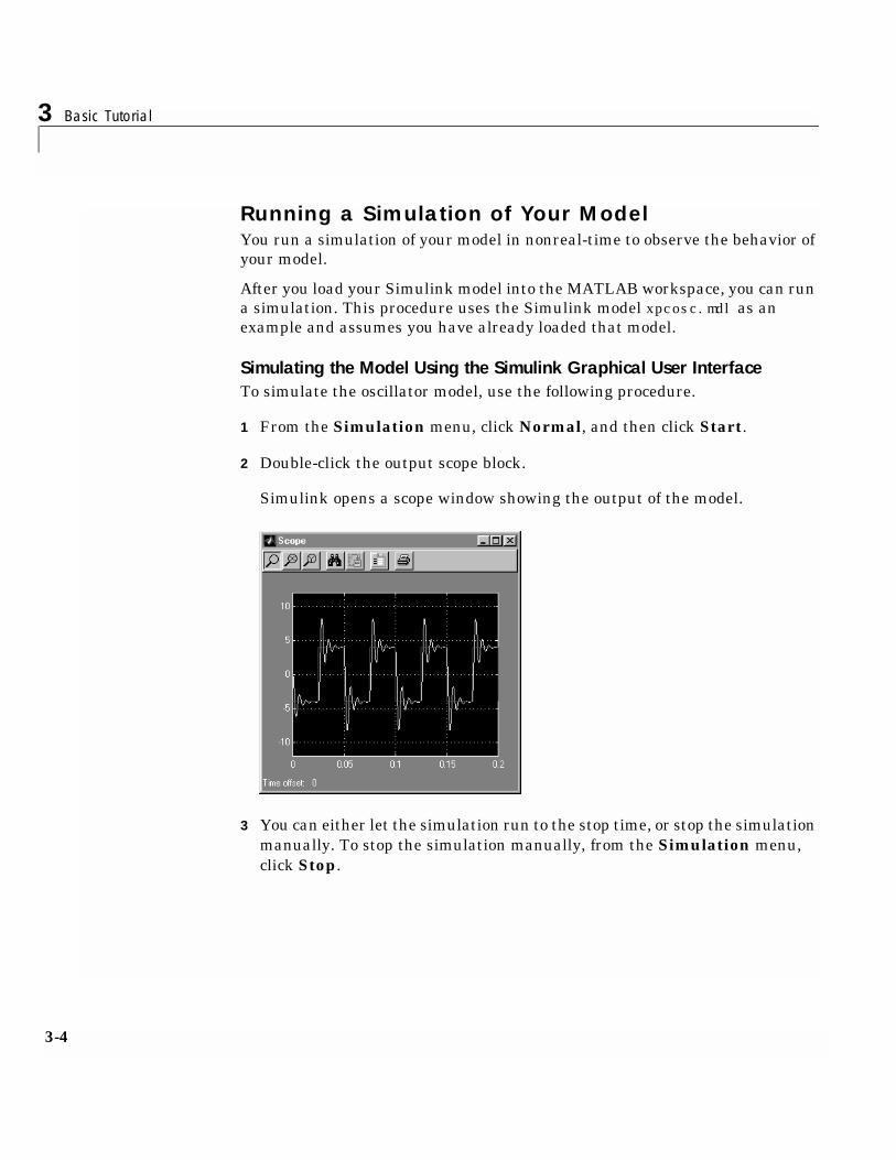
1 From the Simulation menu, click Normal, and then click Start.
2 Double-click the output scope block.
Simulink opens a scope window showing the output of the model.
3 You can either let the simulation run to the stop time, or stop the simulationmanually. To stop the simulation manually, from the Simulation menu,click Stop.
Running a Simulation on the Host PC
3-5
Simulating the model using the MATLAB command line interfaceTo simulate the oscillator model, use the following procedure.
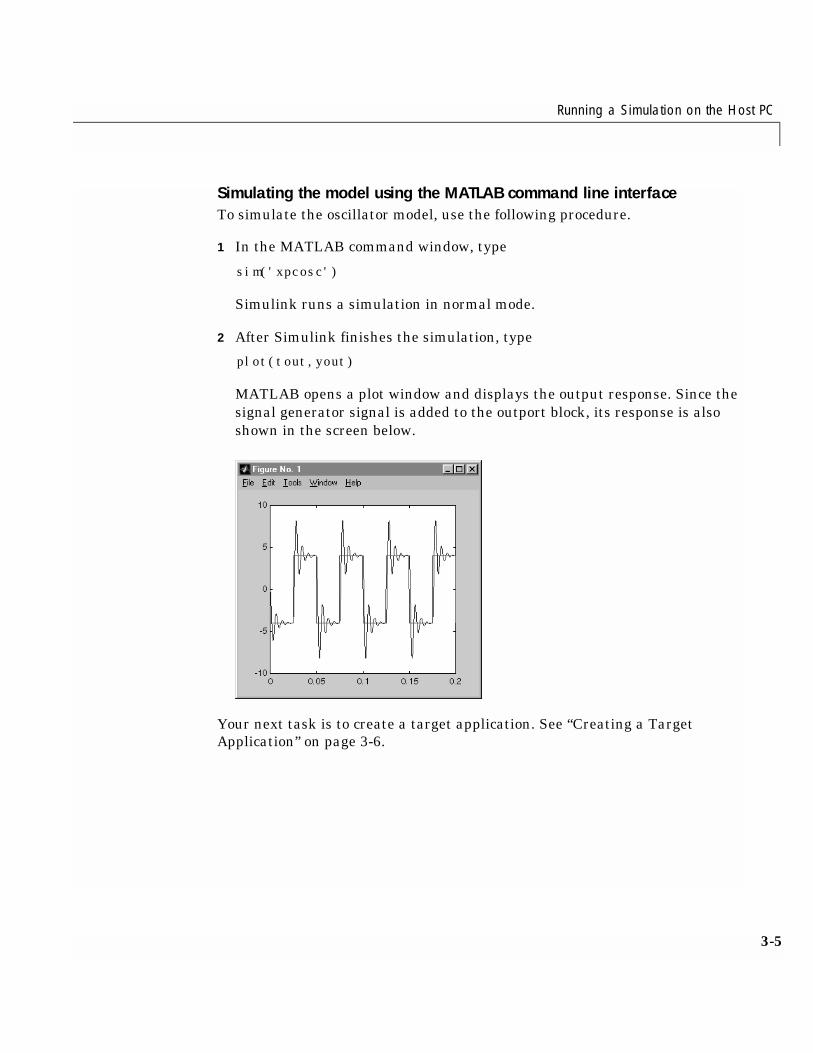
1 In the MATLAB command window, type
sim('xpcosc')
Simulink runs a simulation in normal mode.
2 After Simulink finishes the simulation, type
plot(tout,yout)
MATLAB opens a plot window and displays the output response. Since thesignal generator signal is added to the outport block, its response is alsoshown in the screen below.
Your next task is to create a target application. See “Creating a TargetApplication” on page 3-6.
3 Basic Tutorial
3-6
Creating a Target ApplicationYou use the target application to observe the behavior of your model inreal-time.
This section includes the following topics:
• “Booting the Target PC”
• “Entering the Simulation Parameters”
• “Building and Downloading the Target Application”
• “Troubleshooting the Build Process”
For procedures to simulate your model in nonreal-time, see “Running aSimulation on the Host PC” on page 3-3.
Booting the Target PCBooting your target computer loads and starts the xPC Target kernel. Theloader then waits for xPC Target to download your target application from yourhost PC to your target PC.
After you have configured xPC Target using the Setup window, and created atarget boot disk for that setup, you can boot your target PC. You need to bootthe target computer before building the target application because the buildprocess automatically downloads the target application to your target PC.
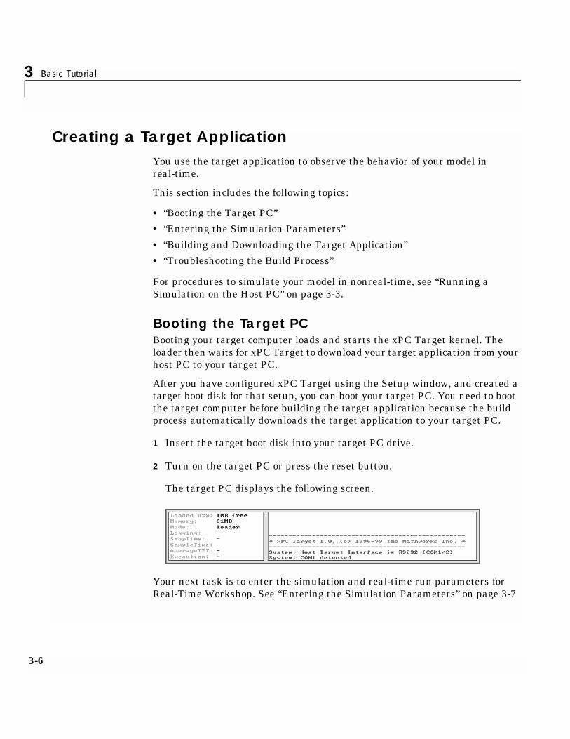
1 Insert the target boot disk into your target PC drive.
2 Turn on the target PC or press the reset button.
The target PC displays the following screen.
Your next task is to enter the simulation and real-time run parameters forReal-Time Workshop. See “Entering the Simulation Parameters” on page 3-7
Creating a Target Application
3-7
Possible Problem. When booting the target PC, it might display the message:
xPC Target 1.0 loading kernel..@@@@@@@@@@@@@@@@@@@@@@
The target PC displays this message when it cannot read and load the kernelfrom the target boot disk. The probable cause is a bad disk.
Solution. The solution is to reformat the disk or use a new preformatted floppydisk and create a new target boot disk.
Entering the Simulation ParametersThe simulation or real-time run parameters are part of Simulink andReal-Time Workshop. They give information to Real-Time Workshop for how itbuilds the target application from your Simulink model.
After you load a Simulink model and boot your target PC, you can enter thesimulation parameters for Real-Time Workshop. This procedure uses theSimulink model xpcosc.mdl as an example and assumes you have alreadyloaded that model.
1 In the Simulink block window, and from the Simulation menu, clickParameters. In the Simulation Parameters dialog box, click the Solvertab.
The Solver property sheet opens.
2 In the Start time box, enter 0 seconds. In the Stop time box, enter 0.2second.
3 From the Type list, choose Fixed-step. From the integration algorithm listchoose ode4 (Runge-Kutta). In the Fixed step size box, enter 0.00025second (250 microseconds).
If you find that 0.000250 second results in overloading the CPU on yourtarget PC, try a slower Fixed step size such as 0.002 second.
3 Basic Tutorial
3-8
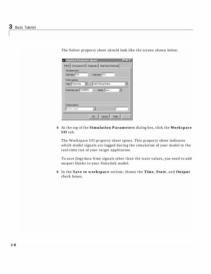
The Solver property sheet should look like the screen shown below.
4 At the top of the Simulation Parameters dialog box, click the WorkspaceI/O tab.
The Workspace I/O property sheet opens. This property sheet indicateswhich model signals are logged during the simulation of your model or thereal-time run of your target application.
To save (log) data from signals other than the state values, you need to addoutport blocks to your Simulink model.
5 In the Save to workspace section, choose the Time, State, and Outputcheck boxes.
Creating a Target Application
3-9
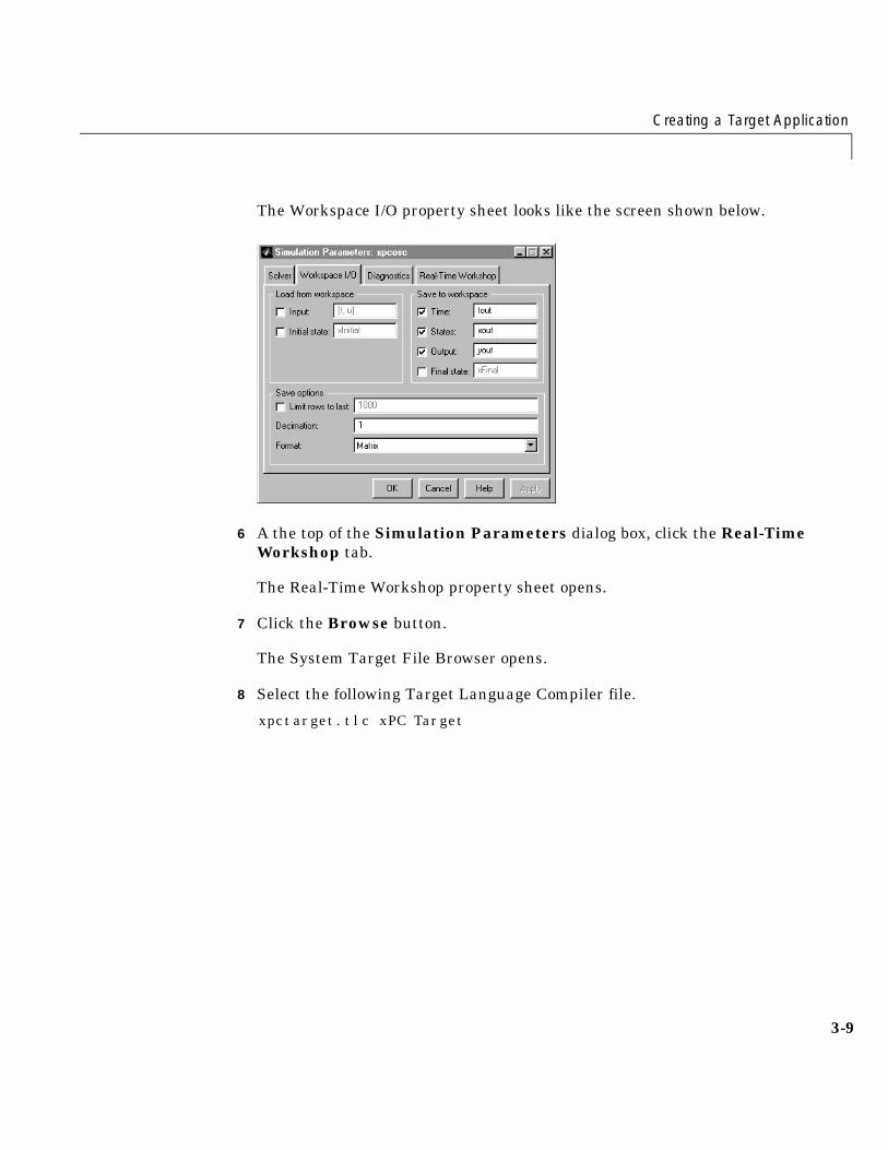
The Workspace I/O property sheet looks like the screen shown below.
6 A the top of the Simulation Parameters dialog box, click the Real-TimeWorkshop tab.
The Real-Time Workshop property sheet opens.
7 Click the Browse button.
The System Target File Browser opens.
8 Select the following Target Language Compiler file.
xpctarget.tlc xPC Target
3 Basic Tutorial
3-10
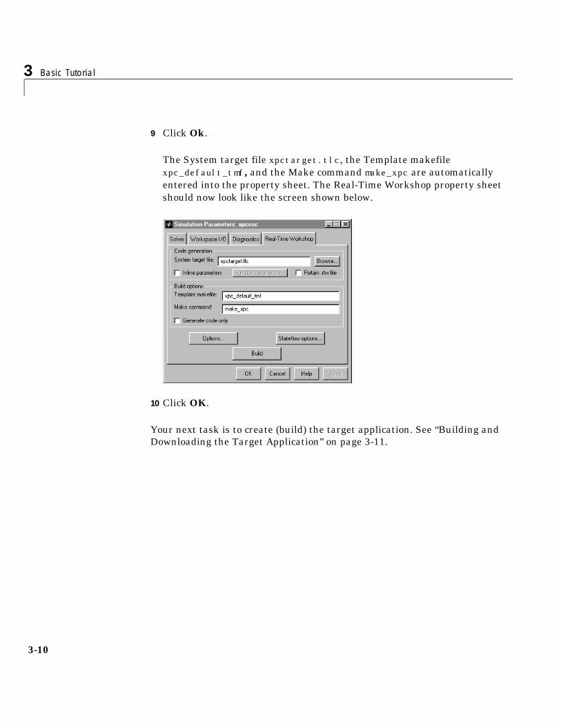
9 Click Ok.
The System target file xpctarget.tlc, the Template makefilexpc_default_tmf, and the Make command make_xpc are automaticallyentered into the property sheet. The Real-Time Workshop property sheetshould now look like the screen shown below.
10 Click OK.
Your next task is to create (build) the target application. See “Building andDownloading the Target Application” on page 3-11.
Creating a Target Application
3-11
Building and Downloading the Target ApplicationYou use the xPC Target build process to generate C code, compile, link, anddownload the target application to your target PC.
After you enter your changes in the Simulation Parameters dialog box, youcan build the target application. This procedure uses the Simulink modelxpcosc.mdl as an example, and assumes you have loaded that model.
1 In the Simulink block window, and from the Tools menu, click RTW Build.
After the compiling, linking, and downloading process, a target object iscreated with properties and associated methods (functions). The defaultname of the target object is tg. For more information about the target object,see “Target Object Properties and Commands” on page 7-4.
On the host computer, the following lines are displayed after a successfulbuild process.
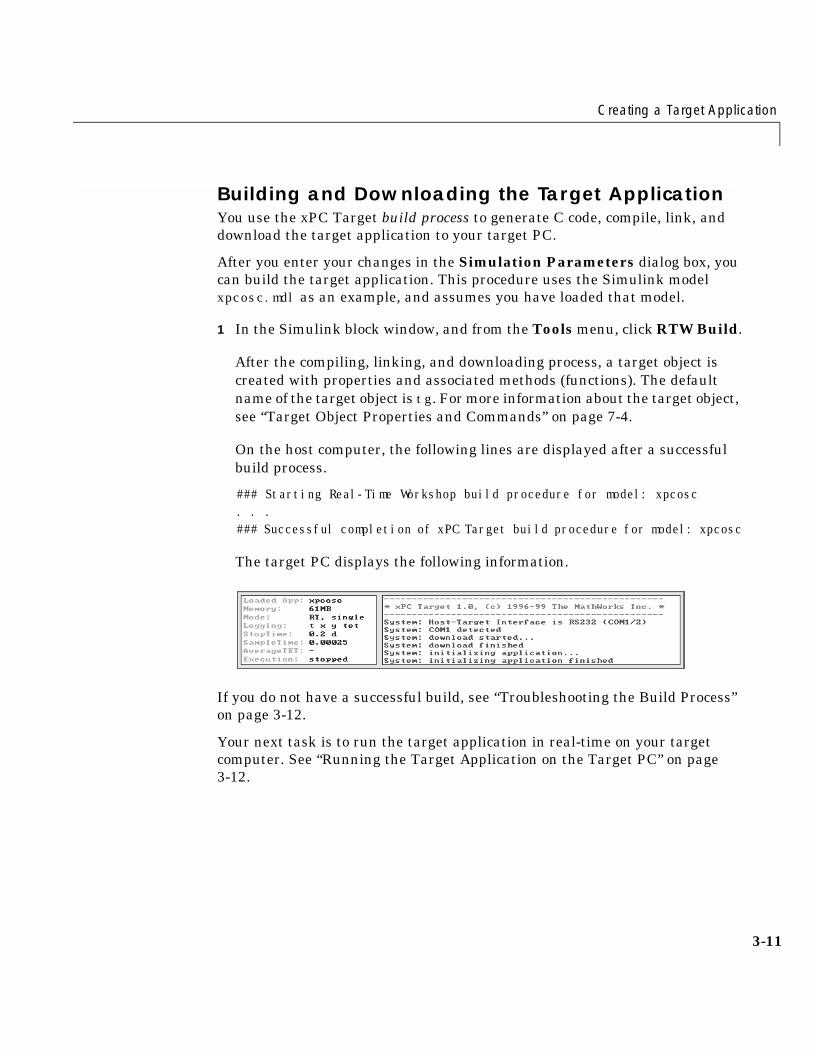
### Starting Real-Time Workshop build procedure for model: xpcosc. . .### Successful completion of xPC Target build procedure for model: xpcosc
The target PC displays the following information.
If you do not have a successful build, see “Troubleshooting the Build Process”on page 3-12.
Your next task is to run the target application in real-time on your targetcomputer. See “Running the Target Application on the Target PC” on page3-12.
3 Basic Tutorial
3-12
Troubleshooting the Build ProcessIf the host PC and target PC are not properly connected or you have notcorrectly entered the properties, the download process is terminated afterabout 5 seconds with a time-out error.
To correct the problem, open the Setup window. In the MATLAB commandwindow, type
xpcsetup
Check and, if necessary, make changes to the communication properties,update the properties, and recreate the target boot disk. For information on theprocedures, see ether “Setting the Environment for Serial Communication” onpage 2-12 or “Setting the Environment for Network Communication” on page2-19, and then see “Creating a Target Boot Disk for the Target PC” on page2-22.
Running the Target Application on the Target PCDuring the build process, a target object was created with properties andassociated commands (methods). You control the target application bychanging the target object properties with the target object commands.
For more detailed information about the target object properties andcommands (methods), see “Target Object Properties and Commands” on page7-4.
This section includes the following topic:
• “Starting and Stopping the Target Application”
Running the Target Application on the Target PC
3-13
Starting and Stopping the Target ApplicationYou run your target application in real time to observe the behavior of yourmodel with generated code.
After xPC Target downloads your target application to your target PC, you canrun the target application. This procedure uses the Simulink modelxpcosc.mdl as an example, and assumes you have created and downloaded thetarget application for that model. The default name of the target object is tg.
1 Start the target application. In the MATLAB command window, type either
start(tg) or +tg
On the host screen, and in the MATLAB command window, the status of thetarget object changes from stopped to running.
xPC ObjectConnected = Yes
Application = xpcosc Mode = Real-Time Single-Tasking Status = running
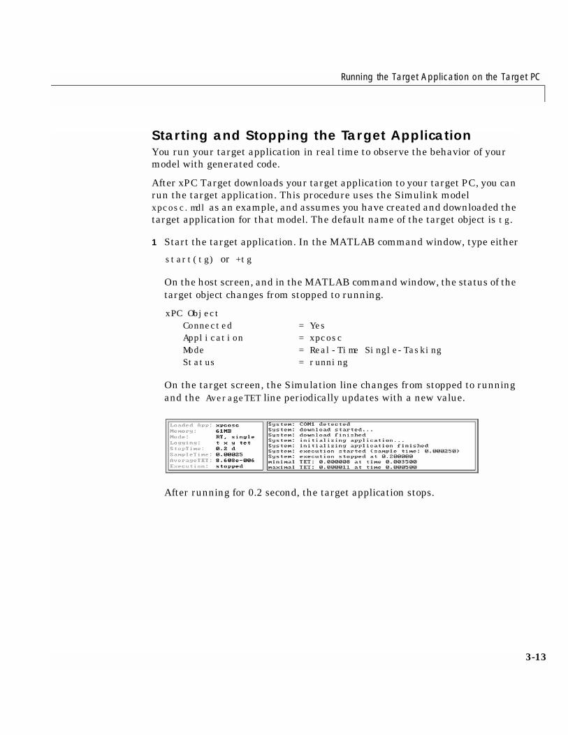
On the target screen, the Simulation line changes from stopped to runningand the AverageTET line periodically updates with a new value.
After running for 0.2 second, the target application stops.
3 Basic Tutorial
3-14
2 Change the final time between runs. For example, to change the stop timeto 1000 seconds, type either
set(tg,'StopTime',1000) or tg.StopTime = 1000
3 Change the sample time between runs. For example, to change the sampletime to 0.01 second, type either
set(tg, 'SampleTime', 0.01) or tg.SampleTime = 0.01
Although you can change the sample time in between different runs, you canonly change the sample time without rebuilding the target application undercertain circumstances.
If you choose a sample time that is too small, a CPU overload can occur. If aCPU overload occurs, the target object property CPU Overload changes todetected. In that case, change the Fixed step size in the Solver propertysheet to a larger value.
4 Restart the simulation. Type either
start(tg) or +tg
5 Stop running the target application. Type either
stop(tg) or -tg
Your next task is to log and observe the signals from your target application inreal-time. See one of the following topics:
• “Signal Logging” on page 3-15
• “Signal Tracing with the Host Scope” on page 3-18
• “Signal Tracing with the Target Scope” on page 3-26
• “Signal Tracing with xPC Target Functions” on page 3-31
Signal Logging
3-15
Signal LoggingSignal logging is the process for acquiring signal data during a real-time run,and after the run reaches its final time or you manually stop the run,transferring the data to the host PC and plotting the data.
Plotting the time, state, and output signals is possible only if you added outportblocks to your Simulink model before the build process, and in the SimulationParameters dialog box, checked the output boxes on theI/O-Workspace property sheet.
Plotting the task execution time is possible only if you checked the LogTETcheck box in the Code Generation Options dialog box. For more information,see “Workspace I/O Properties” on page 6-4 and “Code Generation Dialog Box”on page 6-8.
This section includes the following topics:
• “Plotting Outputs and States”
• “Plotting Task Execution Time”
Plotting Outputs and StatesYou plot the outputs and states of your target application to observe thebehavior of your model, or to determine the behavior when you vary the inputsignal.
After you run a target application, you can plot the state and output signals.This procedure uses the Simulink model xpcosc.mdl as an example, andassumes you have created and downloaded the target application for thatmodel.
1 In the MATLAB command window, type either
start(tg) or +tg
The target application starts and runs until it reaches the Final Time.
The outputs are those signals connected to Simulink outport blocks. Themodel xpcosc.mdl has just one outport block labeled 1 and there are twostates. This outport block shows the signal leaving the block labeledIntegrator1 and Signal Generator.
3 Basic Tutorial
3-16
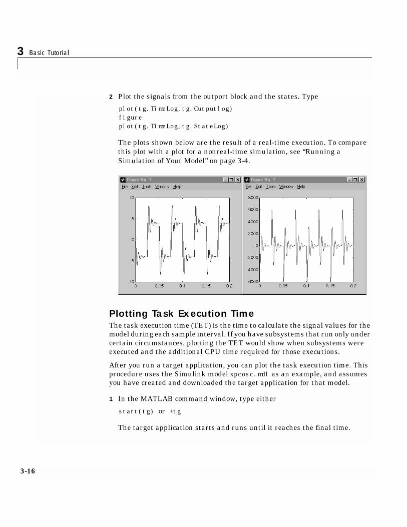
2 Plot the signals from the outport block and the states. Type
plot(tg.TimeLog,tg.Outputlog)figureplot(tg.TimeLog,tg.StateLog)
The plots shown below are the result of a real-time execution. To comparethis plot with a plot for a nonreal-time simulation, see “Running aSimulation of Your Model” on page 3-4.
Plotting Task Execution TimeThe task execution time (TET) is the time to calculate the signal values for themodel during each sample interval. If you have subsystems that run only undercertain circumstances, plotting the TET would show when subsystems wereexecuted and the additional CPU time required for those executions.
After you run a target application, you can plot the task execution time. Thisprocedure uses the Simulink model xpcosc.mdl as an example, and assumesyou have created and downloaded the target application for that model.
1 In the MATLAB command window, type either
start(tg) or +tg
The target application starts and runs until it reaches the final time.
Signal Logging
3-17
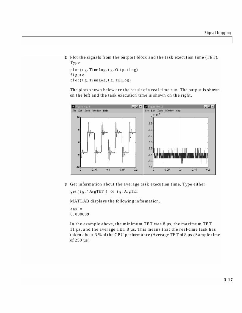
2 Plot the signals from the outport block and the task execution time (TET).Type
plot(tg.TimeLog,tg.Outputlog)figureplot(tg.TimeLog,tg.TETLog)
The plots shown below are the result of a real-time run. The output is shownon the left and the task execution time is shown on the right.
3 Get information about the average task execution time. Type either
get(tg,'AvgTET') or tg.AvgTET
MATLAB displays the following information.
ans =0.000009
In the example above, the minimum TET was 8 µs, the maximum TET11 µs, and the average TET 8 µs. This means that the real-time task hastaken about 3 % of the CPU performance (Average TET of 8 µs / Sample timeof 250 µs).
3 Basic Tutorial
3-18
Signal Tracing with the Host ScopeSignal tracing is the process of acquiring and visualizing signals during areal-time run. It allows you to acquire signal data and visualize it on yourtarget PC or upload the signal data and visualize it on your host PC while thetarget application is running.
Signal logging differs from signal tracing. With signal logging you can only lookat a signal after a run is finished, and the entire log of the run is available. Forinformation on signal logging, see “Signal Logging” on page 3-15.
With xPC Target, signal tracing is called Scope because this function is similarto using a digital oscilloscope. You can access the Scope functions indirectlythrough a Scope window, or directly by using xPC Target commands.
This section includes the following topics:
• “Creating a Scope Object and Selecting Signals”
• “Exporting Data from the Host Scope Window”
• “Closing All Scope Windows”
For procedures on using xPC Target commands for scopes, see “Signal Tracingwith xPC Target Functions” on page 3-31.
Signal Tracing with the Host Scope
3-19
Creating a Scope Object and Selecting SignalsOpening a Scope window allows you to view signals with a graphical userinterface (GUI).
After you create, download, and start running a target application, you canview signals. This procedure uses the Simulink model xpcosc.mdl as anexample, and assumes you are running the target application for that model.
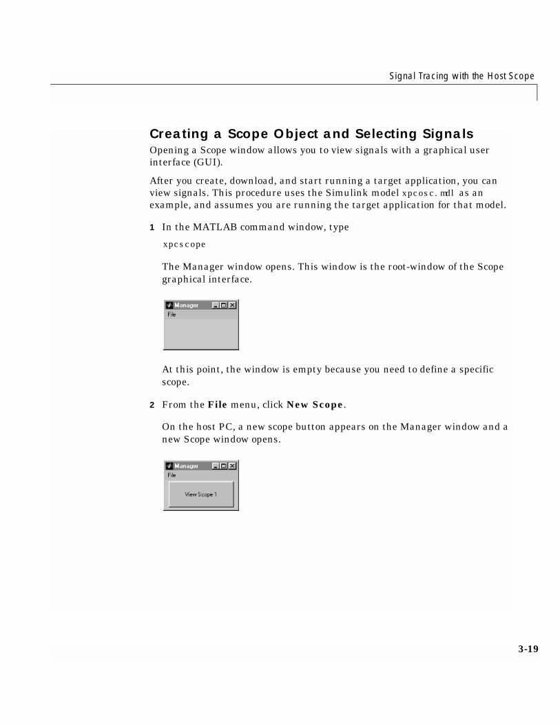
1 In the MATLAB command window, type
xpcscope
The Manager window opens. This window is the root-window of the Scopegraphical interface.
At this point, the window is empty because you need to define a specificscope.
2 From the File menu, click New Scope.
On the host PC, a new scope button appears on the Manager window and anew Scope window opens.
3 Basic Tutorial
3-20
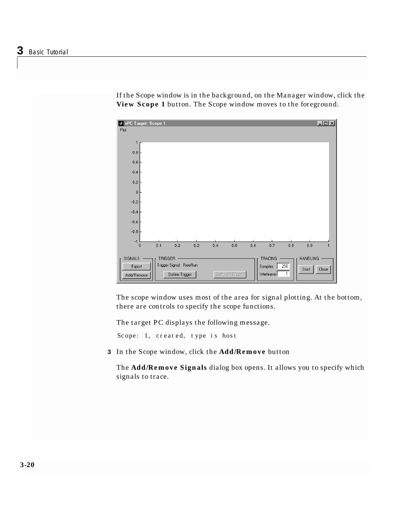
If the Scope window is in the background, on the Manager window, click theView Scope 1 button. The Scope window moves to the foreground.
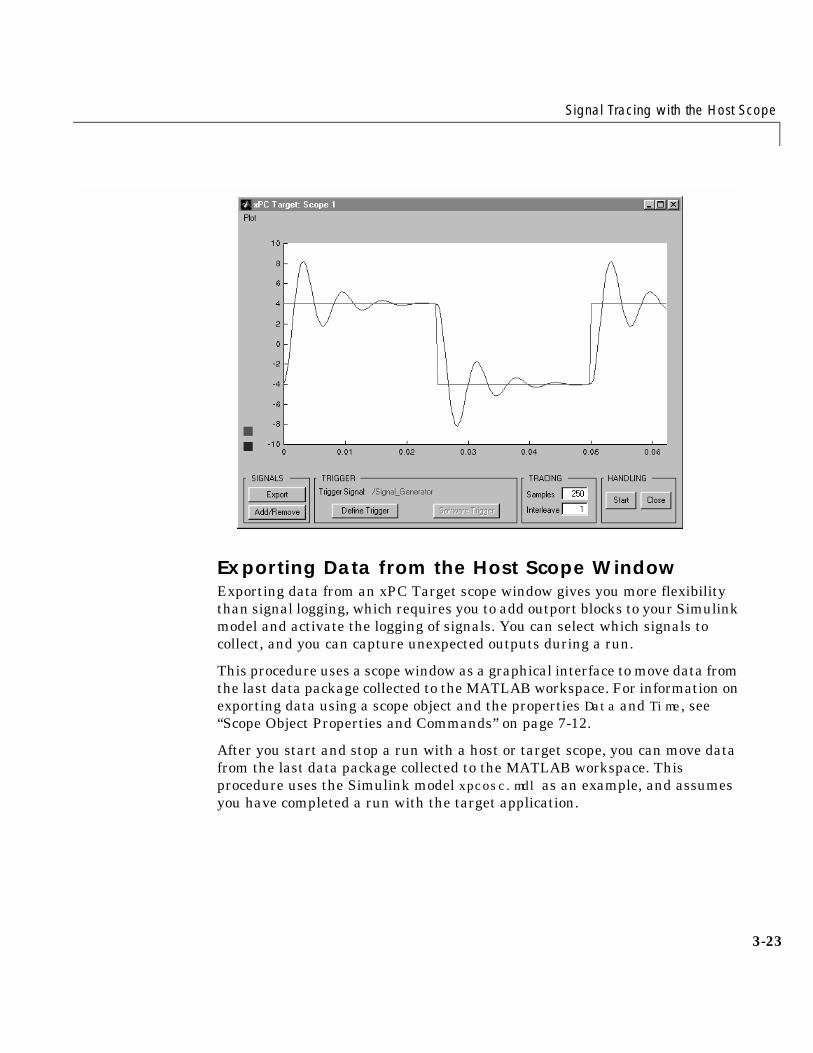
The scope window uses most of the area for signal plotting. At the bottom,there are controls to specify the scope functions.
The target PC displays the following message.
Scope: 1, created, type is host
3 In the Scope window, click the Add/Remove button
The Add/Remove Signals dialog box opens. It allows you to specify whichsignals to trace.
Signal Tracing with the Host Scope
3-21
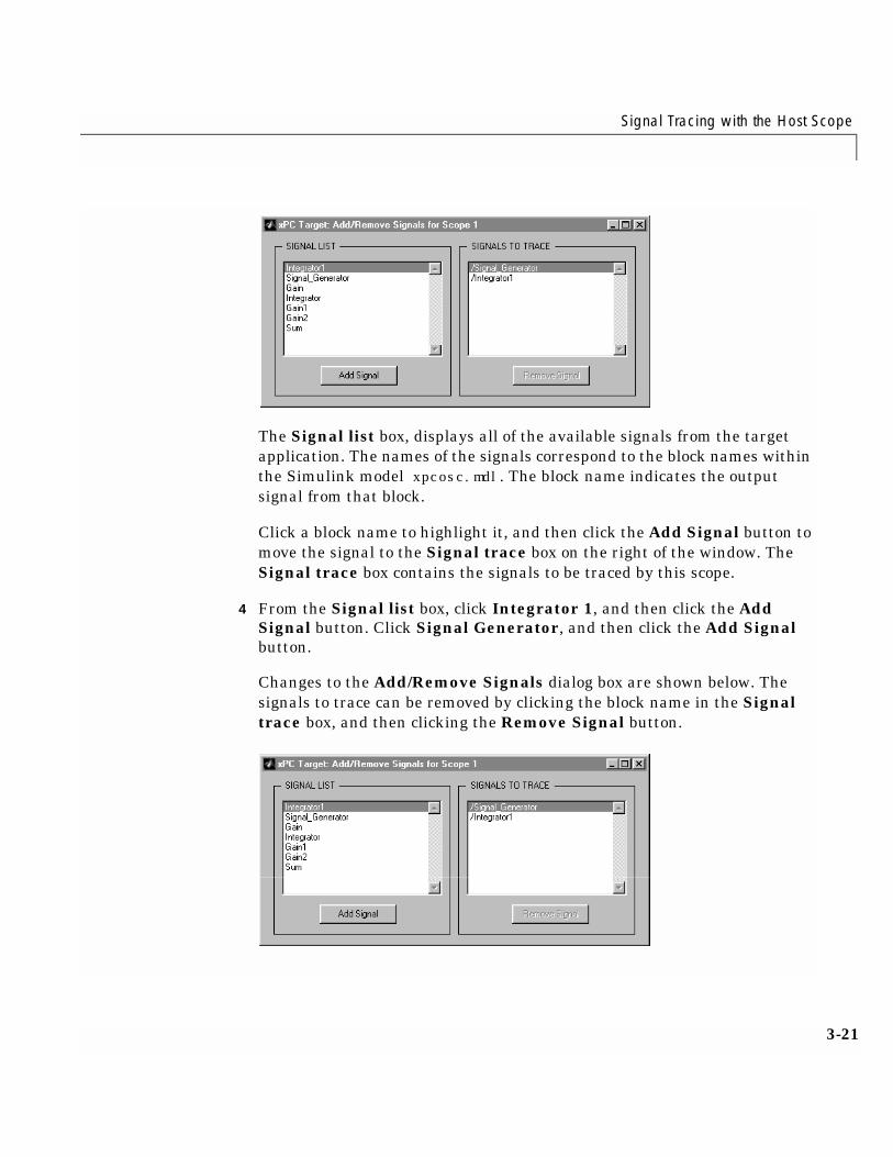
The Signal list box, displays all of the available signals from the targetapplication. The names of the signals correspond to the block names withinthe Simulink model xpcosc.mdl. The block name indicates the outputsignal from that block.
Click a block name to highlight it, and then click the Add Signal button tomove the signal to the Signal trace box on the right of the window. TheSignal trace box contains the signals to be traced by this scope.
4 From the Signal list box, click Integrator 1, and then click the AddSignal button. Click Signal Generator, and then click the Add Signalbutton.
Changes to the Add/Remove Signals dialog box are shown below. Thesignals to trace can be removed by clicking the block name in the Signaltrace box, and then clicking the Remove Signal button.
3 Basic Tutorial
3-22
During the next steps, you can leave the Add/Remove Signals dialog boxopen, or close and reopen it without restrictions.
You can now start the scope. You also need to start a run before the signalsare visible in the scope window. If you use a scope, set the final time to avalue high enough to ensure the target application is running during theentire signal tracing session. The final time is set by changing the targetobject property StopTime.
5 In the Scope window, click the Start button. In the MATLAB commandwindow, type either
start(tg) or +tg
The target application starts running.
You can start the scope and the target application in any order. The targetapplication does not have to be running to start the scope or make changesto the scope properties. While the scope is running, the Start button on theScope window changes to a Stop button.
If a target application is running and you start a scope, the host scopewindow acquires one data package, and then updates the signal graph. Thetime to collect one data package is equal to the number of samples multipliedby the sample time.
If you are using a host scope, there is a delay between collecting datapackages because of the communication overhead from your target to hostcomputers. If you are using a target scope, the target scope window isupdated faster than when using a host scope.
Signal Tracing with the Host Scope
3-23
Exporting Data from the Host Scope WindowExporting data from an xPC Target scope window gives you more flexibilitythan signal logging, which requires you to add outport blocks to your Simulinkmodel and activate the logging of signals. You can select which signals tocollect, and you can capture unexpected outputs during a run.
This procedure uses a scope window as a graphical interface to move data fromthe last data package collected to the MATLAB workspace. For information onexporting data using a scope object and the properties Data and Time, see“Scope Object Properties and Commands” on page 7-12.
After you start and stop a run with a host or target scope, you can move datafrom the last data package collected to the MATLAB workspace. Thisprocedure uses the Simulink model xpcosc.mdl as an example, and assumesyou have completed a run with the target application.
3 Basic Tutorial
3-24
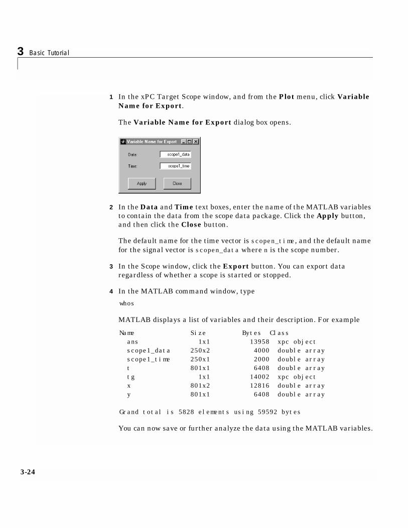
1 In the xPC Target Scope window, and from the Plot menu, click VariableName for Export.
The Variable Name for Export dialog box opens.
2 In the Data and Time text boxes, enter the name of the MATLAB variablesto contain the data from the scope data package. Click the Apply button,and then click the Close button.
The default name for the time vector is scopen_time, and the default namefor the signal vector is scopen_data where n is the scope number.
3 In the Scope window, click the Export button. You can export dataregardless of whether a scope is started or stopped.
4 In the MATLAB command window, type
whos
MATLAB displays a list of variables and their description. For example
Name Size Bytes Class ans 1x1 13958 xpc object scope1_data 250x2 4000 double array scope1_time 250x1 2000 double array t 801x1 6408 double array tg 1x1 14002 xpc object x 801x2 12816 double array y 801x1 6408 double array
Grand total is 5828 elements using 59592 bytes
You can now save or further analyze the data using the MATLAB variables.
Signal Tracing with the Host Scope
3-25
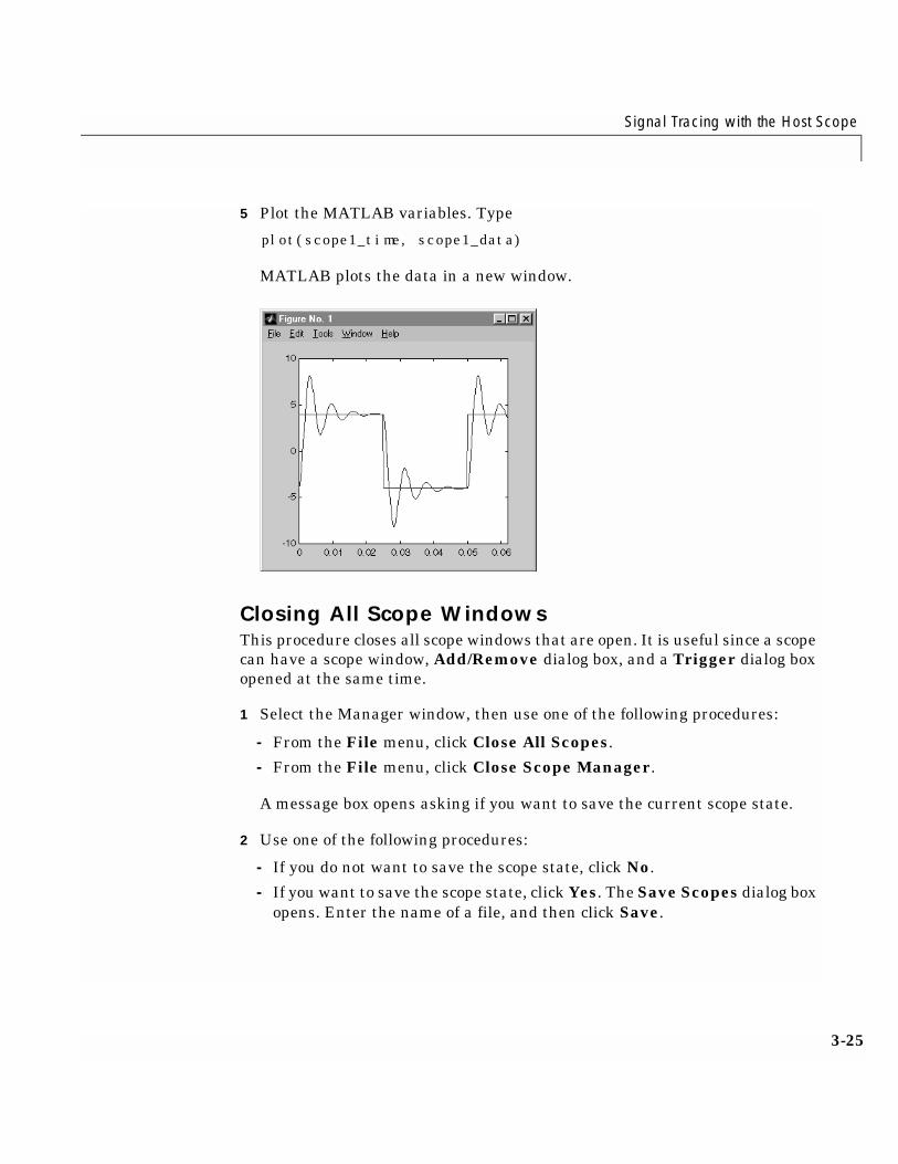
5 Plot the MATLAB variables. Type
plot(scope1_time, scope1_data)
MATLAB plots the data in a new window.
Closing All Scope WindowsThis procedure closes all scope windows that are open. It is useful since a scopecan have a scope window, Add/Remove dialog box, and a Trigger dialog boxopened at the same time.
1 Select the Manager window, then use one of the following procedures:
- From the File menu, click Close All Scopes.
- From the File menu, click Close Scope Manager.
A message box opens asking if you want to save the current scope state.
2 Use one of the following procedures:
- If you do not want to save the scope state, click No.
- If you want to save the scope state, click Yes. The Save Scopes dialog boxopens. Enter the name of a file, and then click Save.
3 Basic Tutorial
3-26
Signal Tracing with the Target ScopeSignal tracing is acquiring signals while a real-time execution is running. Itallows you to acquire signals and visualize them on the target PC.
This section includes the following topic:
• “Creating a Target Scope Object and Selecting Signals”
For a discussion of signal tracing and a brief description of a scope object, see“Signal Tracing with the Host Scope” on page 3-18.
Creating a Target Scope Object and Selecting SignalsOpening a target scope window allows you to select and view signals using agraphical user interface.
After you create, download, and start running a target application, you canview signals. This procedure uses the Simulink model xpcosc.mdl as anexample, and assumes you are running the target application for that model.
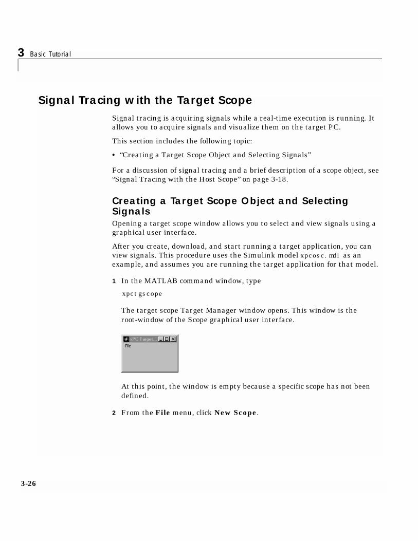
1 In the MATLAB command window, type
xpctgscope
The target scope Target Manager window opens. This window is theroot-window of the Scope graphical user interface.
At this point, the window is empty because a specific scope has not beendefined.
2 From the File menu, click New Scope.
Signal Tracing with the Target Scope
3-27
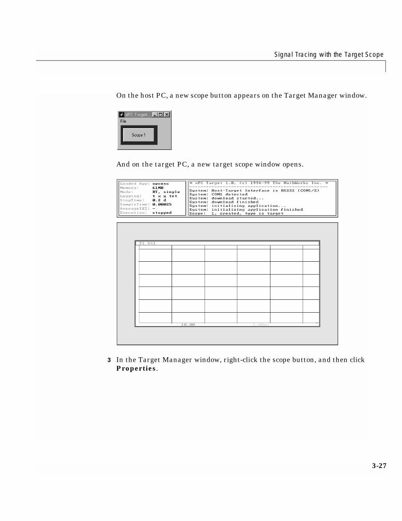
On the host PC, a new scope button appears on the Target Manager window.
And on the target PC, a new target scope window opens.
3 In the Target Manager window, right-click the scope button, and then clickProperties.
3 Basic Tutorial
3-28
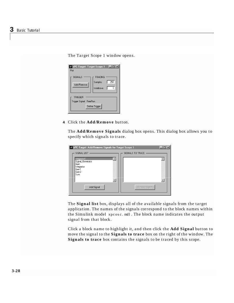
The Target Scope 1 window opens.
4 Click the Add/Remove button.
The Add/Remove Signals dialog box opens. This dialog box allows you tospecify which signals to trace.
The Signal list box, displays all of the available signals from the targetapplication. The names of the signals correspond to the block names withinthe Simulink model xpcosc.mdl. The block name indicates the outputsignal from that block.
Click a block name to highlight it, and then click the Add Signal button tomove the signal to the Signals to trace box on the right of the window. TheSignals to trace box contains the signals to be traced by this scope.
Signal Tracing with the Target Scope
3-29
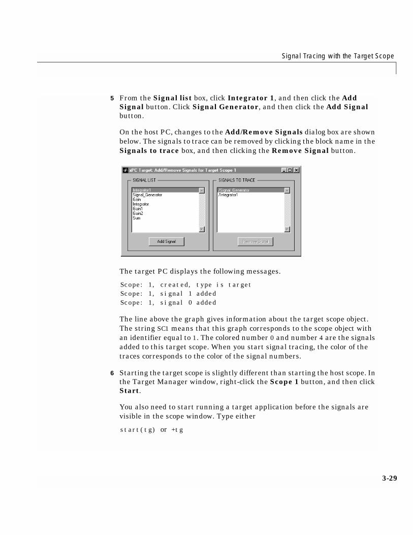
5 From the Signal list box, click Integrator 1, and then click the AddSignal button. Click Signal Generator, and then click the Add Signalbutton.
On the host PC, changes to the Add/Remove Signals dialog box are shownbelow. The signals to trace can be removed by clicking the block name in theSignals to trace box, and then clicking the Remove Signal button.
The target PC displays the following messages.
Scope: 1, created, type is targetScope: 1, signal 1 addedScope: 1, signal 0 added
The line above the graph gives information about the target scope object.The string SC1 means that this graph corresponds to the scope object withan identifier equal to 1. The colored number 0 and number 4 are the signalsadded to this target scope. When you start signal tracing, the color of thetraces corresponds to the color of the signal numbers.
6 Starting the target scope is slightly different than starting the host scope. Inthe Target Manager window, right-click the Scope 1 button, and then clickStart.
You also need to start running a target application before the signals arevisible in the scope window. Type either
start(tg) or +tg
3 Basic Tutorial
3-30
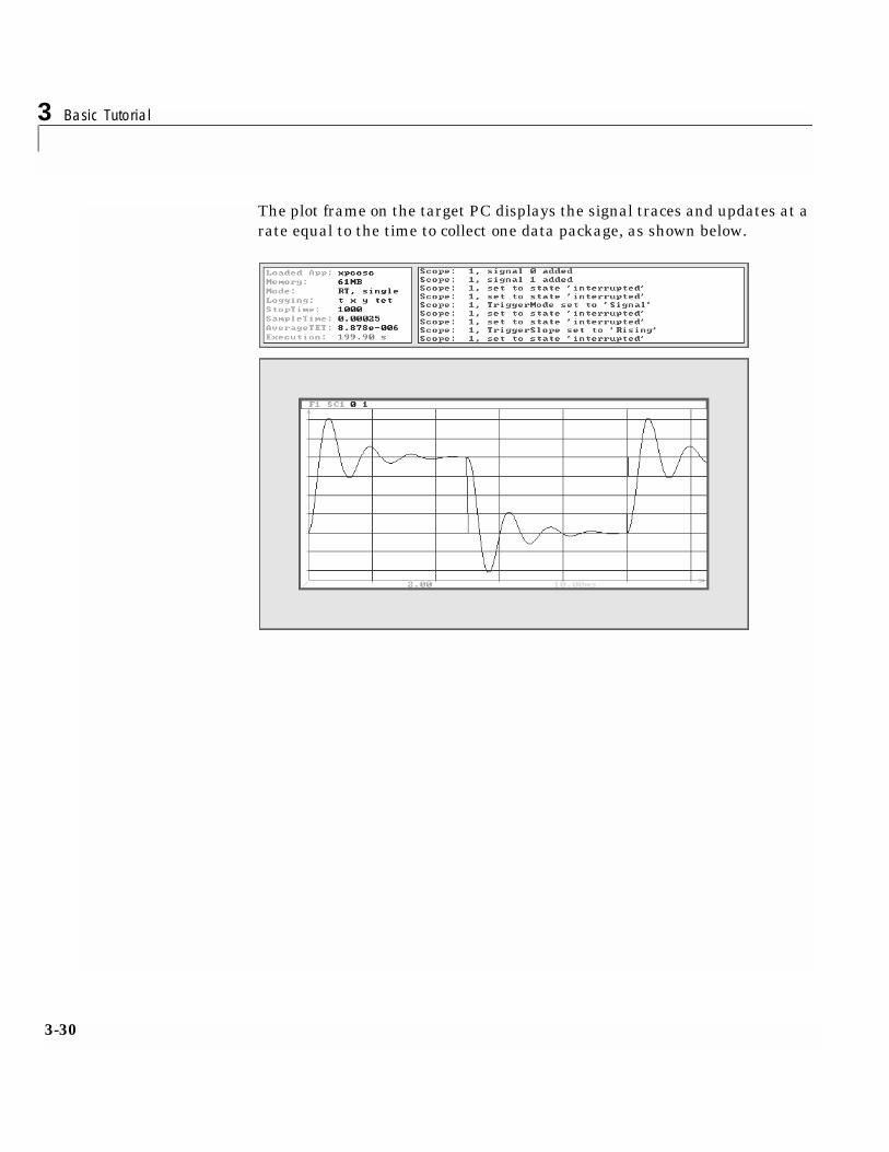
The plot frame on the target PC displays the signal traces and updates at arate equal to the time to collect one data package, as shown below.

Signal Tracing with xPC Target Functions
3-31
Signal Tracing with xPC Target FunctionsSignal tracing is acquiring signals while a real-time execution is running. Itallows you to acquire signals and visualize them on the target PC.
This section describes how to signal trace using xPC Target functions insteadof using the xPC Target graphical interface.
This section includes the following topic:
• “Creating a Target Scope Object and Selecting Signals”
For a discussion of signal tracing with a graphical user interface and a briefdescription of a scope object, see “Signal Tracing with the Host Scope” on page3-18.
Creating a Target Scope Object and Selecting SignalsCreating a target scope object allows you to select and view signals using thexPC Target functions.
After you create and download, the target application, you can view outputsignals. This procedure uses the Simulink model xpcosc.mdl as an example,and assumes you have build the target application for that model.
1 Increase the stop time. For example, to increase the stop time to 1000seconds, in the MATLAB command window, type
tg.stoptime=1000
1 Start running your target application. Type either
start(tg) or +tg
The target PC displays the following message.
System: simulation started (sample time: 0.0000250)
2 To get a list of parameters, type either
set(tg, 'ShowSignals', 'on') or tg.ShowSignals='on'
3 Basic Tutorial
3-32
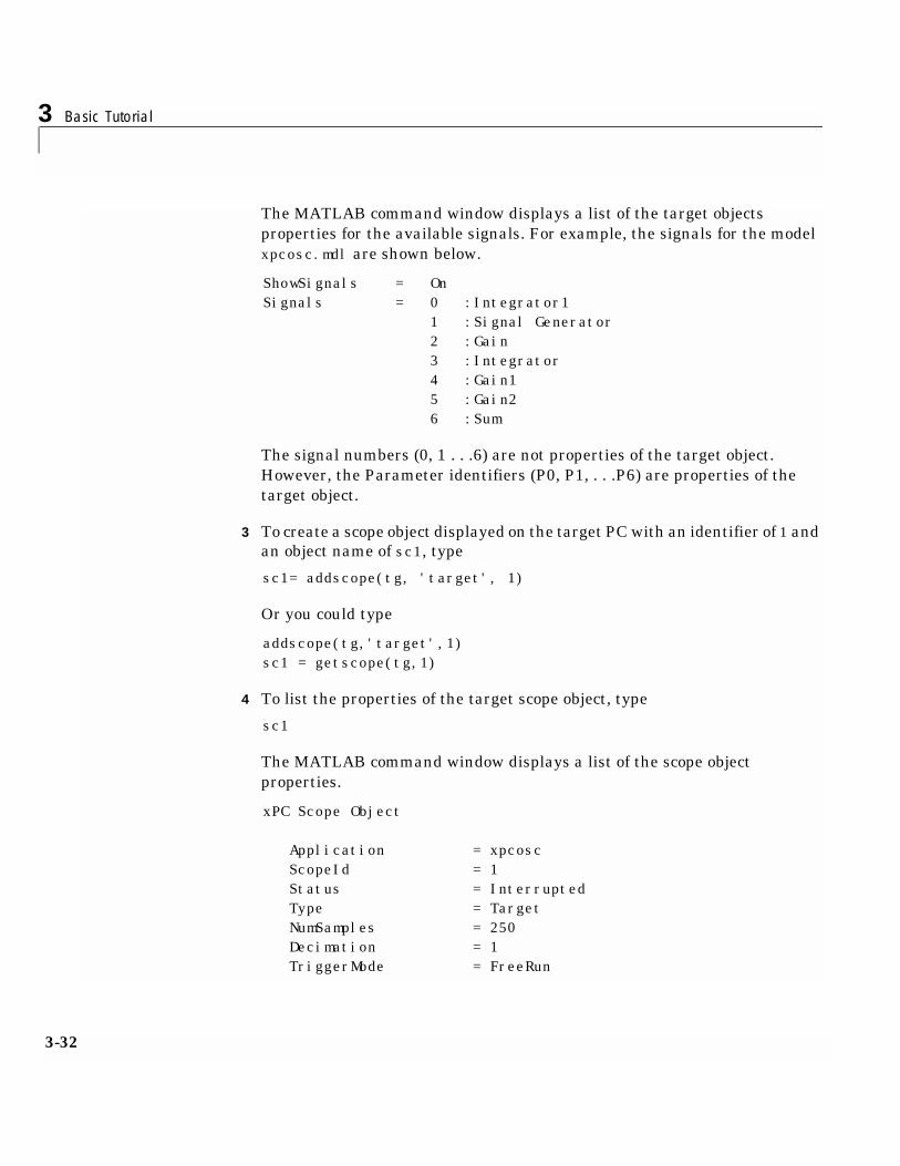
The MATLAB command window displays a list of the target objectsproperties for the available signals. For example, the signals for the modelxpcosc.mdl are shown below.
ShowSignals = OnSignals = 0 :Integrator1
1 :Signal Generator2 :Gain3 :Integrator4 :Gain15 :Gain26 :Sum
The signal numbers (0, 1 . . .6) are not properties of the target object.However, the Parameter identifiers (P0, P1, . . .P6) are properties of thetarget object.
3 To create a scope object displayed on the target PC with an identifier of 1 andan object name of sc1, type
sc1= addscope(tg, 'target', 1)
Or you could type
addscope(tg,'target',1)sc1 = getscope(tg,1)
4 To list the properties of the target scope object, type
sc1
The MATLAB command window displays a list of the scope objectproperties.
xPC Scope Object
Application = xpcosc ScopeId = 1 Status = Interrupted Type = Target NumSamples = 250 Decimation = 1 TriggerMode = FreeRun
Signal Tracing with xPC Target Functions
3-33
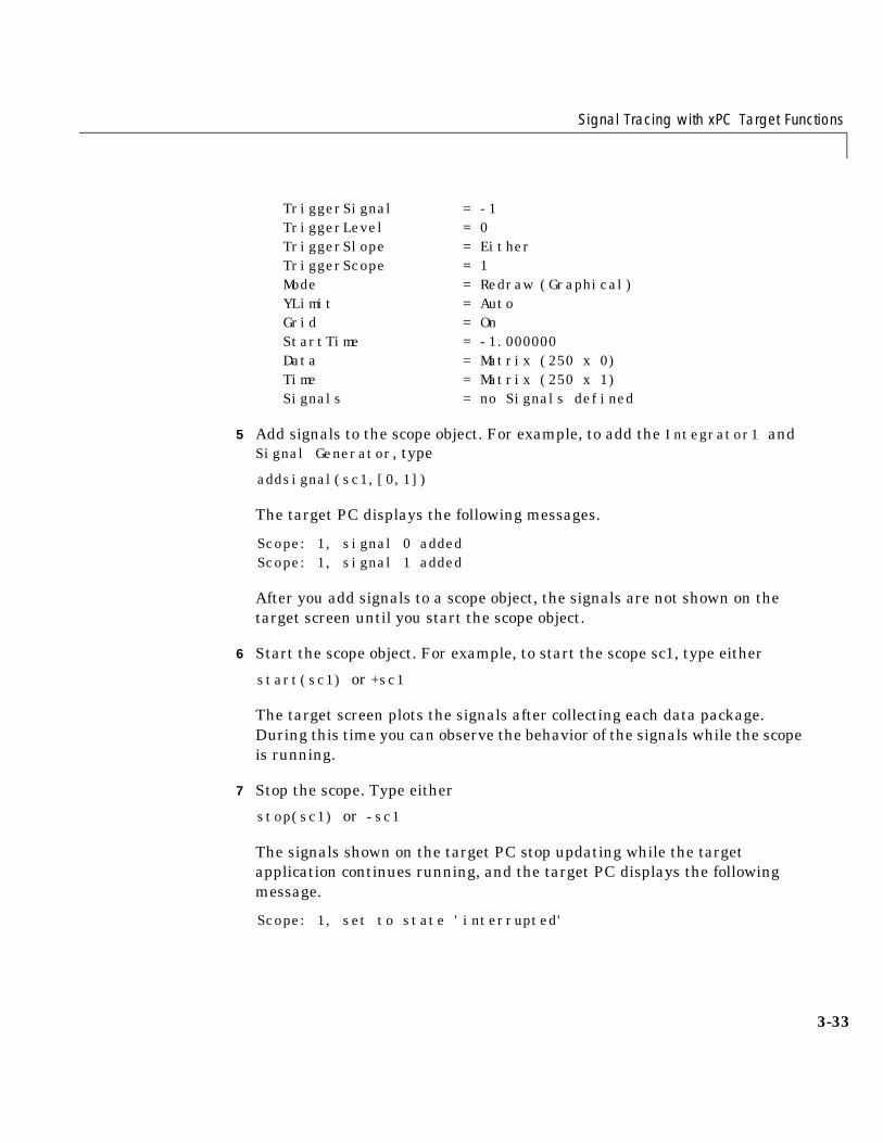
TriggerSignal = -1 TriggerLevel = 0 TriggerSlope = Either TriggerScope = 1 Mode = Redraw (Graphical) YLimit = Auto Grid = On StartTime = -1.000000 Data = Matrix (250 x 0) Time = Matrix (250 x 1) Signals = no Signals defined
5 Add signals to the scope object. For example, to add the Integrator1 andSignal Generator, type
addsignal(sc1,[0,1])
The target PC displays the following messages.
Scope: 1, signal 0 addedScope: 1, signal 1 added
After you add signals to a scope object, the signals are not shown on thetarget screen until you start the scope object.
6 Start the scope object. For example, to start the scope sc1, type either
start(sc1) or +sc1
The target screen plots the signals after collecting each data package.During this time you can observe the behavior of the signals while the scopeis running.
7 Stop the scope. Type either
stop(sc1) or -sc1
The signals shown on the target PC stop updating while the targetapplication continues running, and the target PC displays the followingmessage.
Scope: 1, set to state 'interrupted'
3 Basic Tutorial
3-34
Parameter Tuning Using Simulink External ModeYou use Simulink external mode to connect your Simulink block diagram toyour target application. The block diagram becomes a graphical user interfaceto your target application where you can change block parameter values andhave those changes also made in your running target application.
This section includes the following topics:
• “What Is External Simulation Mode?”
• “Setting Up Simulink in External Mode”
Alternately, you can use xPC Target commands instead of using the Simulinkwindow to change model parameters. You usually use these functions toprogram and batch process a series of runs. For an introduction to thesecommands, see “Parameter Tuning with xPC Target Commands” on page 3-38
What Is External Simulation Mode?External simulation mode is a feature of the Real-Time Workshop (RTW). Itoffers an easy way to change parameters in a target application regardlesswhether a target application is running or not:
• If a target application is not running, it allows you to prepare a model witha new set of parameters before the next run.
• If a target application is running, it allows you to change parameters andimmediately see what effect changing parameters has on the behavior ofyour generated code.
After installing the Real-Time Workshop, the Simulink window has new menucommands and dialog boxes that relate to the external simulation mode:
• On the Simulation menu there are two new commands: Normal andExternal.
By selecting normal mode, Simulink is able to run a nonreal-time simulationof your model on your host PC. See “Running a Simulation on the Host PC”on page 3-3. You start and stop the nonreal-time simulation by using theStart and Stop commands from the Simulation menu.
Parameter Tuning Using Simulink External Mode
3-35
By selecting external mode, Simulink is able to make a connection to yourtarget application running on the target PC. This communication channelallows you to use a Simulink block diagram as a graphical user interface tothe target application.
The menu item Parameters opens the Simulations Parameters dialogbox and selects the RTW Workshop tab.
• On the Tools menu there are three new commands: RTW Build, RTWOptions, and External Mode Control Panel.
Setting Up Simulink in External ModeYou set up Simulink in external mode to establish a communication channelbetween your Simulink block window and your target application.
After you download your target application to your target PC, you can connectyour Simulink model to the target application.
1 In the Simulink block window, and from the Simulation menu, clickExternal.
A check mark appears next to the menu item External, and Simulinkexternal mode is activated.
2 In the Simulink block window, and from the Simulation menu, clickConnect to Target.
All of the current Simulink model parameters are downloaded to your targetapplication. This downloading guarantees the consistency of the parametersbetween the host model and the target application.
The target PC displays the following message.
ExtM: Updating # parameters
Your next task is to change parameters using Simulink external mode, see“Changing the Target Object Properties” on page 3-38.
3 Basic Tutorial
3-36
Changing Simulink Block ParametersIn Simulink external mode, wherever you change parameters in the Simulinkblock diagram, Simulink downloads those parameters to the target applicationwhile it is running. This feature lets you change parameters in your programwithout rebuilding the Simulink model to create a new target application.
After you have downloaded a target application to your target PC, and set upSimulink in external mode, you can change parameters in your targetapplication by changing parameters in your Simulink model. This procedureuses the Simulink model xpcosc.mdl as an example, and assumes you havecreated and downloaded the target application for that model.
3 From the Simulation menu, click Start Real-Time Code or in theMATLAB command window, type either
start(tg) or +tg
The target application begins running on the target PC, and the target PCdisplays the following message.
System: execution started (sample time: 0.000250)
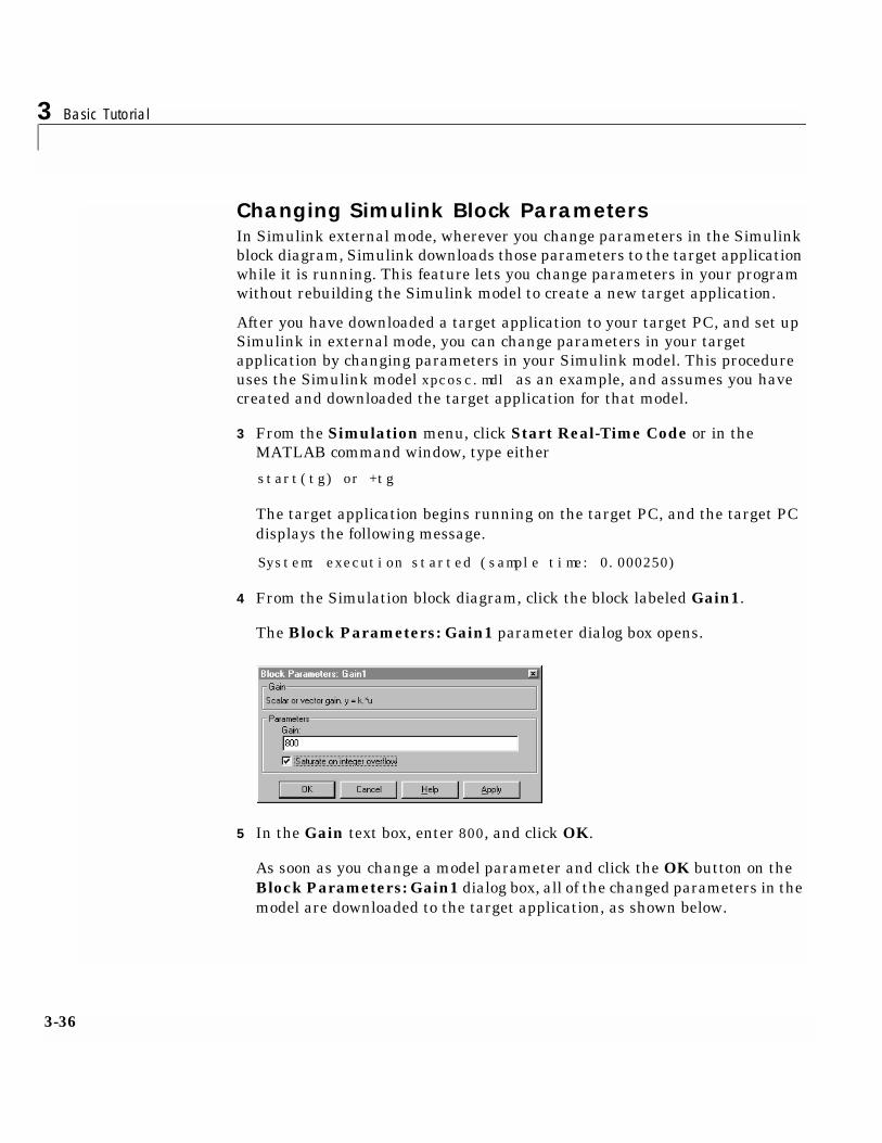
4 From the Simulation block diagram, click the block labeled Gain1.
The Block Parameters: Gain1 parameter dialog box opens.
5 In the Gain text box, enter 800, and click OK.
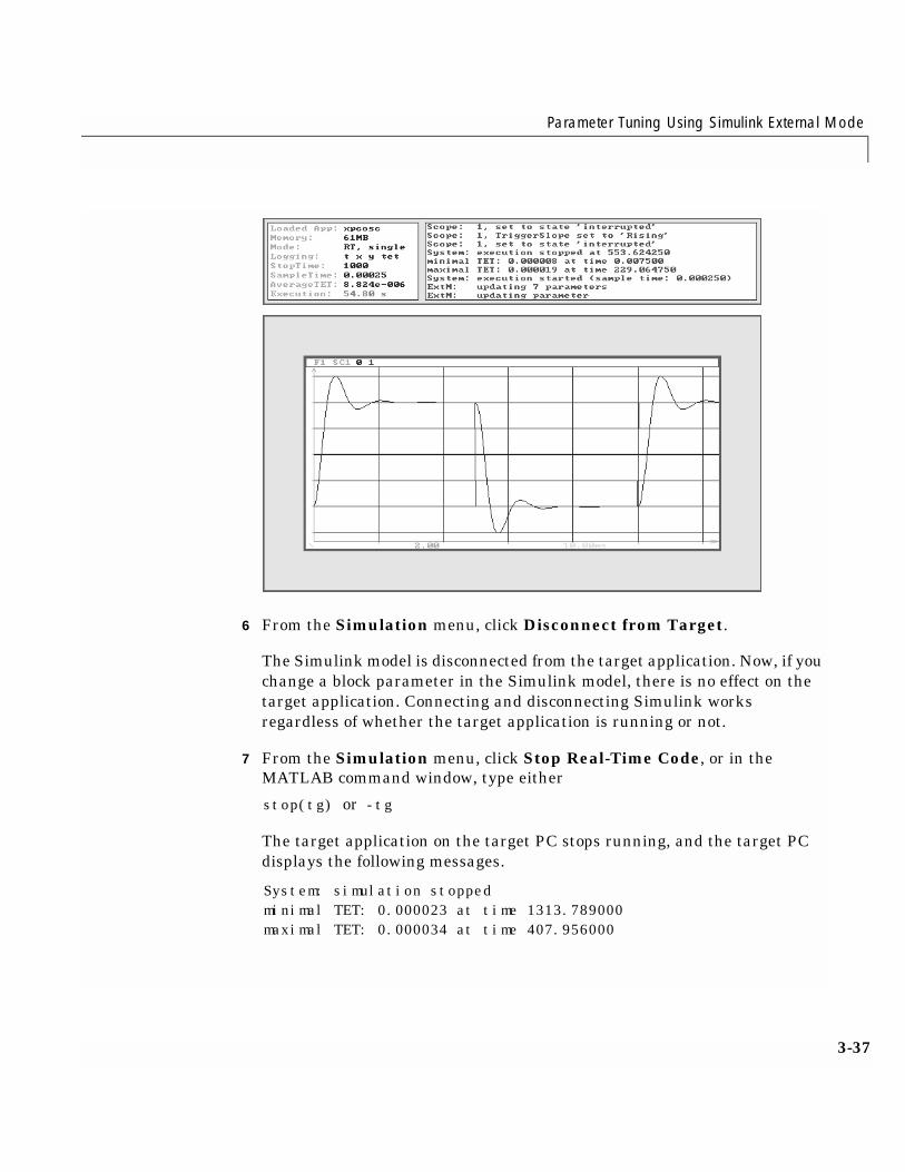
As soon as you change a model parameter and click the OK button on theBlock Parameters: Gain1 dialog box, all of the changed parameters in themodel are downloaded to the target application, as shown below.
Parameter Tuning Using Simulink External Mode
3-37
6 From the Simulation menu, click Disconnect from Target.
The Simulink model is disconnected from the target application. Now, if youchange a block parameter in the Simulink model, there is no effect on thetarget application. Connecting and disconnecting Simulink worksregardless of whether the target application is running or not.
7 From the Simulation menu, click Stop Real-Time Code, or in theMATLAB command window, type either
stop(tg) or -tg
The target application on the target PC stops running, and the target PCdisplays the following messages.
System: simulation stoppedminimal TET: 0.000023 at time 1313.789000maximal TET: 0.000034 at time 407.956000
3 Basic Tutorial
3-38
Parameter Tuning with xPC Target CommandsYou use the xPC Target functions to change block parameters. You do not needto set Simulink in external mode, and you do not need to connect Simulink withthe target application. You enter the xPC Target functions in the MATLABcommand window, and they work whether the target application is running, orit is stopped.
This section includes the following topic:
• “Changing the Target Object Properties” on page 3-38
Alternately, you can also use the Simulink window as a graphical interface tothe target application instead of using xPC Target commands. You use thisgraphical interface to interactively change parameters during a run. For anintroduction to Simulink external mode, see “Parameter Tuning UsingSimulink External Mode” on page 3-34.
Changing the Target Object PropertiesYou can download parameters to the target application while it is running orbetween runs. This feature lets you change parameters in your programwithout rebuilding the Simulink model.
After you download a target application to the target PC, you can change blockparameters using xPC Target functions. This procedure uses the Simulinkmodel xpcosc.mdl as an example, and assumes you have created anddownloaded the target application for that model.
1 In the MATLAB command window, type either
start(tg) or +tg
The target PC displays the following message.
System: execution started (sample time: 0.001000)
2 Display a list of parameters. Type either
set(tg, 'ShowParameters', 'on') or tg.ShowParameters='on'tg
Parameter Tuning with xPC Target Commands
3-39
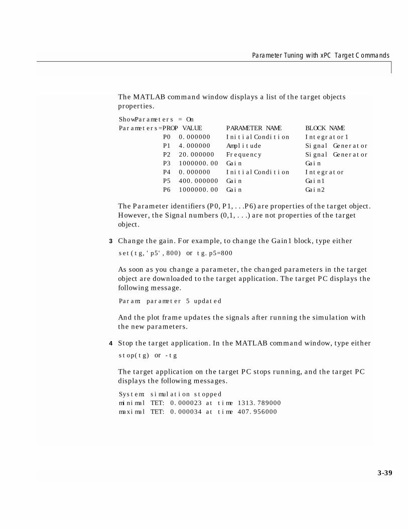
The MATLAB command window displays a list of the target objectsproperties.
ShowParameters = OnParameters=PROP VALUE PARAMETER NAME BLOCK NAME
P0 0.000000 InitialCondition Integrator1P1 4.000000 Amplitude Signal GeneratorP2 20.000000 Frequency Signal GeneratorP3 1000000.00 Gain GainP4 0.000000 InitialCondition IntegratorP5 400.000000 Gain Gain1P6 1000000.00 Gain Gain2
The Parameter identifiers (P0, P1, . . .P6) are properties of the target object.However, the Signal numbers (0,1, . . .) are not properties of the targetobject.
3 Change the gain. For example, to change the Gain1 block, type either
set(tg,'p5',800) or tg.p5=800
As soon as you change a parameter, the changed parameters in the targetobject are downloaded to the target application. The target PC displays thefollowing message.
Param: parameter 5 updated
And the plot frame updates the signals after running the simulation withthe new parameters.
4 Stop the target application. In the MATLAB command window, type either
stop(tg) or -tg
The target application on the target PC stops running, and the target PCdisplays the following messages.
System: simulation stoppedminimal TET: 0.000023 at time 1313.789000maximal TET: 0.000034 at time 407.956000

3 Basic Tutorial
3-40