Preferences and Utility.

X : set of alternatives (choice set or domain).

A preference relation % is a binary relation on X thatallows comparison of pairs of alternatives x, y ∈ X.

x % y : alternative x is at least as good as alternative y.

From %, we can derive two other binary preference rela-tions on X:

(i) Strict preference relation � defined by

x � y ⇔ x % y but not y % x

(ii) Indifference relation ∼ defined by

x ∼ y ⇔ x % y and y % x

A basic assumption on % that underlies much of eco-nomics is that it is rational.

Definition: The preference relation % on X is rational ifit satisfies the following properties:

(1) Completeness: for all x, y ∈ X, either x % y ory % x or both.

(2) Transitivity:for all x, y, z ∈ X, if x % y and y % z,then x % z.

Sometimes a rational preference relation is also called an"ordering".

Question:

If the weak preference relation % on X is complete, doesit imply that the strict preference relation � and the in-difference relation ∼ are complete?

If the weak preference relation % on X is transitive, doesit imply that the strict preference relation � and the in-difference relation ∼ are transitive?

Utility Function.

A utility function assigns a numerical value to each ele-ment in X in accordance with the preference.

More formally:

Definition: A function u : X → R is a utility functionrepresenting preference relation % if, for all x, y ∈ X,

x % y ⇔ u(x) ≥ u(y).

A utility function representing a preference relation % isnot unique.

Exercise: If u represents % on X, then for any strictlyincreasing function f : R → R, v(x) = f(u(x)) is alsoa utility function that represents % .

Note: v is then said to be a strictly increasing transfor-mation of u.

Properties of utility function that are invariant for allstrictly increasing transformations are known as ordinalproperties.

Otherwise, they are cardinal properties.

Exercise: If u represents %, then for all x, y ∈ X,

x � y ⇔ u(x) > u(y)

and

x ∼ y ⇔ u(x) = u(y).

Proposition (1.B.2): A preference relation % can berepresented by a utility function only if it is rational.

Proof: Suppose there exists a utility function u thatrepresents % on X.

For any pair x, y ∈ X, either

u(x) ≥ u(y) or u(y) ≥ u(x) (or both)

and since u that represents %, this must imply:

x % y or y % x (or both)which shows that % is complete.

Next, we show% is transitive. Suppose x % y and y % z.We need to show that x % z.

As u that represents %, this must imply:

u(x) ≥ u(y) and u(y) ≥ u(z)

so that

u(x) ≥ u(z)

which implies (again because u that represents %)

x % z.Thus, % is transitive. The proof is complete.

Not every rational preference relation can be representedby a utility function.

Example: Lexicographic preferences (Example 3.C.1in textbook)

X = R2+. For any pair of alternatives x, y ∈ X, where

x = (x1, x2), y = (y1, y2),

x % y if either x1 > y1, or x1 = y1 and x2 ≥ y2.

Verify that this particular preference is rational.

Suppose that there is a utility function u that representsthis preference.

For every non-negative real number z we can look at thereal numbers u(z, 1) and u(z, 2).

Now, from the definition of lexicographic preferences, ob-serve that (z, 2) % (z, 1) but not (z, 1) % (z, 2) whichimplies (z, 2) � (z, 1).

Hence (see exercise above):

u(z, 2) > u(z, 1).

Between any distinct real numbers there is a rationalnumber. So, for every non-negative real number z thereexists a rational number r(z) such that

u(z, 2) > r(z) > u(z, 1).

Further, from the definition of lexicographic ordering ifz > z′, then

(z, 2) � (z, 1) � (z′, 2) � (z′, 1)

which implies

u(z, 2) > r(z) > u(z, 1) > u(z′, 2) > r(z′) > u(z′, 1).

Thus, for every non-negative real number z there existsa distinct rational number r(z).

But there are uncountable positive real numbers but onlycountably many rational numbers. A contradiction.

Exercise: If X is finite, then every rational preference re-lation can be represented by a utility function.

Consumer Behavior and Walrasian Demand.

L commodities, l = 1, 2, ...L.

L finite.

A commodity vector (bundle) lists amounts of the differ-

ent commodities : x =

x1x2..xL

xl : consumption level of good l

Consumption Set X ⊂ RL: Set of all consumption bun-dles that the consumer can conceivably consume giventhe physical constraints.

Assume: X = RL+

(Any non-negative bundle may be consumed)

Consumer’s preference relation % defined on X = RL+.

Notation:

For vectors x =

x1x2..xL

,y =

y1y2..yL

,

y � x⇐⇒ yl > xl, for all l = 1, ...L,

y ≥ x⇐⇒ yl ≥ xl, for all l = 1, ...L,

Note,

y ≥ x, y 6= x⇐⇒ yl ≥ xl, for all l and yl > xl, for some l.

Euclidean norm: For x ∈ RL, ‖x‖ =

√√√√ L∑l=1

(xl)2

Euclidean distance: For x, y ∈ RL, the (Euclidean) dis-tance between vectors x and y is given by ‖x− y‖ =√√√√ L∑l=1

(xl − yl)2

Some common assumptions on % used in classical de-mand theory:

Desirability assumptions:

Definition: The preference relation % is monotone ifx ∈ X and y � x implies y � x.

Definition: The preference relation% is strongly monotoneif x ∈ X and y ≥ x, y 6= x implies y � x.

(These imply goods are "good"; no "bads").

Definition: The preference relation % satisfies local non-satiation if for every x ∈ X and every ε > 0, there isy ∈ X such that ‖ y − x ‖< ε and y � x.

(Implies that arbitrarily close to any consumption bundle,there is a better bundle).

Exercise (Exercise 3.B.1) : Strong monotone⇒Monotone⇒ Local Non-satiation

A digression:

For any x ∈ X,the set {y ∈ x : y % x} is called theupper contour set of x; it is the set of all bundles thatare at least as good as x.

For any x ∈ X,the set {y ∈ x : x % y} is called thelower contour set of x.

For any x ∈ X,the set {y ∈ x : x ∼ y} is called theindifference set x.

Local non-satiation rules out "thick" indifference sets.

Convexity:

A set S ⊂ RL is convex if for all x, y ∈ S and α ∈ [0, 1],

αx+ (1− α)y ∈ S.

(the entire line segment connecting x and y is containedin the set S).

Beware: Convexity of a set is a very different conceptfrom convexity of a function.

Note: X = RL+ is a convex set.

Convexity assumptions:

Definition: The preference relation % is convex if forevery x ∈ X, the upper contour set of x is convex i.e.,for all y, z ∈ X such that y % x and z % x, and for allα ∈ [0, 1],

αy + (1− α)z % x.

Definition: The preference relation % is strictly convexif for every x ∈ X, and for all y, z ∈ X such that y % x,z % x, y 6= z, and for all α ∈ (0, 1),

αy + (1− α)z � x.

Convexity captures a taste for diversification. Implies di-minishing marginal rates of substitution between any pairof goods.

For L = 2, implies that indifference curves are convex tothe origin.

Continuity assumption:

Definition: The preference relation % is continuous if forany sequence of pairs of commodity bundles {(xn, yn)}∞n=1,xn ∈ X, yn ∈ X for all n,with xn % yn for all n,x = limn→∞ xn, y = limn→∞ yn, we have x % y.

(No reversal of preferences in the limit).

Digression: A set S ⊂ RL is said to be closed if the limitof every sequence of vectors in S is contained in S.

Equivalent definition of continuity: For all x ∈ X, theupper and lower contour sets are closed.

Example (Example 3.C.1): Lexicographic preferences arenot continuous.

xn = (1n, 0) � yn = (0, 1) for all n ≥ 1, xn →

(0, 0), yn → (0, 1) but (0, 1) � (0, 0).

Proposition 3.C.1: Suppose that the rational preferencerelation is % on X is continuous. Then there is a con-tinuous utility function that represents % .

(Does not mean that all utility functions representing thepreference relation are continuous)

"Proof": Assume in addition that % is monotone.

Let e ∈ RL+ be the vector (1, 1, 1, ...1).

For every x ∈ RL+, monotone property implies

x % 0

and for any positive number α such that αe� x,

αe % x.

The sets A+ = {α ∈ R+ : αe % x} and A− = {α ∈R+ : x % αe} are nonempty and closed (why?).

Further, as % is complete, for every α ∈ R+, eitherαe % x or x % αe so that α ∈ A+ ∪A−.

Thus, A+ ∪A− = R+.

One mathematical property of R+ is that it is a connectedset which means it cannot be the union of two disjoint,nonempty, closed sets.

So, A+ ∩A− 6= φ.

So there exists α ≥ 0 such that αe % x and x % αe

i.e., αe ∼ x.

By monotonicity, α1e � α2e if α1 > α2.

Therefore, there can be only one real number α(x) suchthat α(x)e ∼ x.

Set u(x) = α(x) for every x ∈ X.

Suppose u(x) ≥ u(y).Then, α(x) ≥ α(y) so that usingmonotonicity of preferences α(x)e % α(y)e. By con-struction, α(x)e ∼ x, α(y)e ∼ y so that using transitiv-ity, x % y.

Conversely, suppose x % y. Then, by construction, α(x)e ∼x, α(y)e ∼ y and so using transitivity α(x)e % α(y)e.

Using monotonicity of preferences, α(x) ≥ α(y) i.e.,u(x) ≥ u(y).

Thus, u(x) ≥ u(y) ⇐⇒ x % y.

So, u represents % .

Continuity of u requires a bit more involved argument.

Assumptions on preferences imply certain properties ofALL utility functions that represent them (they are ordinalproperties).

Monotone % ⇒ u is increasing i.e., u(x) > u(y) ifx� y.

Exercise: Strong monotone % ⇒ ?

Let S ⊂ RL be a convex set.

A function f : S → R is said to be quasiconcave if forall x ∈ S,the set {y ∈ S : f(y) ≥ f(x)} is a convexset; or alternatively, for all x, y ∈ S, α ∈ [0, 1],

f(αx+ (1− α)y) ≥ min{f(x), f(y)}.

A function f : S → R is said to be strictly quasiconcaveif for all x, y ∈ S, x 6= y, α ∈ (0, 1),

f(αx+ (1− α)y) > min{f(x), f(y)}.

% convex ⇒ u is quasi-concave.

% strictly convex ⇒ u is strictly quasi-concave.

Exercise: quasi-concavity is an ordinal property (invariantto any strictly increasing transformation of u).

Let S ⊂ RL be a convex set.

A function f : S → R is said to be concave if for allx, y ∈ S, α ∈ [0, 1],

f(αx+ (1− α)y) ≥ αf(x) + (1− α)f(y).

Concavity ⇒ Quasi-concavity

A function f : S → R is said to be strictly concave if forall x, y ∈ S, x 6= y, α ∈ (0, 1),

f(αx+ (1− α)y) > αf(x) + (1− α)f(y).

Strict concavity ⇒ Strict Quasi-concavity

Concavity of the utility function is not an ordinal property.Not invariant to strictly increasing transformations.

It is not based on any property of the underlying prefer-ence structure.

Law of diminishing marginal utility (implied by concavity,but not necessarily by quasi-concavity) is not an ordinalproperty.

The Utility Maximization Problem

Assume: % is a rational, continuous and locally non-satiated preference relation represented by a continuousutility function u(x) on X = RL+.

We also assume:

(i) the L commodities are all traded in the market atdollar prices that are publicly quoted (complete marketsassumption). In particular, price vector

p =

p1p2..pL

� 0

(ii) consumers are price taking.

Affordability of a commodity bundle depends on pricevector p ∈ RL++ and wealth w ∈ R++.

Definition: The Walrasian, or competitive budget setBp,w = {x ∈ X : p • x ≤ w} is the set of all fea-sible consumption bundles for the consumer who facesmarket prices p and has wealth w.

The upper boundary of the budget set {x ∈ X : p •x =

w} is called the budget hyperplane (or budget line for thecase L = 2).

Digression:

A set S ⊂ RL is said to be bounded if there existsN > 0

such ‖x‖ < N for all x ∈ S.

A set S ⊂ RL is compact if it is both closed and bounded.

Exercise: Bp,w is a compact and convex set.

Utility Maximization Problem (UMP):

Given p� 0 and w > 0,

maxx∈X

u(x)

subject to p • x ≤ w.

or equivalently,

maxx∈Bp,w

u(x).

Weirstrass’ Theorem: Let f : K → R be a continu-ous function and K is a compact set. Then, there existsx′, x′′ ∈ K such that

f(x′) ≤ f(x) ≤ f(x′′) for all x ∈ K.

In other words, f attains a maximum and a minimum inthe set K.

Proposition 3.D.1: If p � 0 and w > 0, then UMPhas a solution.

The proof follows from continuity of u and compactnessof Bp,w.

Note: Solution need not be unique.

Let x(p, w) = {x′ ∈ Bp,w : u(x′) ≥ u(x) for all x ∈Bp,w}

In other words, x(p, w) is the set of all solutions to theUMP.

We can view x(p, w) a set valued mapping or a corre-spondence that associates a set of optimal consumptionbundles with each (p, w). We call this the Walrasian de-mand correspondence.

If x(p, w) is single valued for each (p, w) i.e., there is aunique solution to UMP for every (p, w), then x(p, w) isa function often called the Walrasian demand function.

Proposition 3.D.2: Suppose that u(.) is a continuousutility function representing a locally non-satiated prefer-ence relation% defined on the consumption setX = RL+.Then the Walrasian demand correspondence x(p, w) hasthe following properties:

(i) Homogeneity of degree zero in (p, w) : x(αp, αw) =

x(p, w) for any p� 0, w > 0 and scalar α > 0.

(ii) Walras’law: p • x = w for all x ∈ x(p, w).

(iii) Convexity/uniqueness: If % is convex so that u isquasiconcave, then x(p, w) is a convex set for every (p, w)�0. If % is strictly convex so that u is strictly quasiconcave,then x(p, w) consists of single point.

Proof.

(i) Homogeneity of degree zero in (p, w) : x(αp, αw) =

x(p, w) for any p� 0, w > 0 and scalar α > 0.

This follows from

{x ∈ X : p • x ≤ w} = {x ∈ X : αp • x ≤ αw}

and therefore, the UMP

maxx∈X

u(x)

subject to p • x ≤ w.

is equivalent to

maxx∈X

u(x)

subject to αp • x ≤ αw.

so that the set of solutions to the two max problems areidentical.

(ii) Walras’law: p • x = w for all x ∈ x(p, w)

For any bundle x such that p•x < w, there exists ε > 0

small enough such that p • x′ < w for all x′ ∈ X suchthat

∥∥x′ − x∥∥ < ε.

Using local non-satiation, there exists x′ such that∥∥x′ − x∥∥ <

ε and x′ � x and as that x′ is in the budget set, it con-tradicts the optimality of x.

(iii)i) Convexity/uniqueness: If % is convex so that uis quasiconcave, then x(p, w) is a convex set for every(p, w)� 0.

If x(p, w) has only one element, then it is trivially a con-vex set. So suppose that there are at least two distinctelements x 6= x′ in x(p, w) i.e., both x, x′ solve UMP.

Let

u(x) = u(x′) = u∗.

For any α ∈ [0, 1],consider the bundle x′′ = αx + (1−α)x′.

As Bp,w is a convex set, x′′ ∈ Bp,w.

As u is quasiconcave,

u(x′′) = u(αx+ (1− α)x′) ≥ min{u(x), u(x′)} = u∗

so that x′′ must also be optimal i.e., x′′ ∈ x(p, w). Thus,x(p, w) is a convex set.

Next we show that if % is strictly convex so that uis strictly quasiconcave, then x(p, w) consists of singlepoint.

Suppose to the contrary that there are at least two dis-tinct solutions to UMP x, x′ ∈ x(p, w), x 6= x′.

Let

u(x) = u(x′) = u∗.

Consider the bundle x′′ = 12x+ 1

2x′.

As Bp,w is a convex set, x′′ ∈ Bp,w.

As u is strictly quasiconcave,

u(x′′) = u(1

2x+

1

2x′) > min{u(x), u(x′)} = u∗

which contradicts the fact that x solves UMP and u∗ isthe maximum utility attainable on Bp,w.

Applications:

Suppose x(p, w) is a differentiable function.

Homogeneity of degree zero of the function xl(p, w) im-plies:

L∑k=1

∂xl∂pk

pk +∂xl∂w

w = 0 for all l = 1, ...L.

If xl(p, w) > 0,dividing through by xl :

L∑k=1

∂xl∂pk

pkxl

+∂xl∂w

w

xl= 0

so that:L∑k=1

εlk(p, w) + εlw(p, w) = 0

where εlk(p, w) is the (cross) price elasticity of demandfor good l with respect to price of good k, εlw(p, w) isthe wealth (or income) elasticity of demand for good l.An equi-proportionate change in all prices and wealth hasno net effect on demand.

Walras Law:

p � x(p, w) = w for all p� 0, w > 0

gives us an identity in p, w.Differentiating through withrespect to pk we have

L∑l=1

∂xl(p, w)

∂pkpl + xk(p, w) = 0 for all k = 1, ...L.

If x(p, w) � 0, multiplying through by pk and dividing

through by w

L∑l=1

∂xl∂pk

pkxl

plxlw

+pkxkw

= 0 for all k = 1, ...L.

so that

L∑l=1

εlk(p, w)bl(p, w) + bk(p, w) = 0 for all k = 1, ...L.

where bl(p, w) = plxlw is the share of expenditure (or

budget share) on good l.

p � x(p, w) = w for all p� 0, w > 0

Differentiating through with respect to w we have

L∑l=1

∂xl(p, w)

∂wpl = 1.

If x(p, w)� 0,

L∑l=1

∂xl∂w

w

xl

plxlw

= 1

so that

L∑l=1

εlw(p, w)bl(p, w) = 1.

Continuity of Demand:

In general, there may not be any continuous demandfunction that one can select from the correspondencex(p, w). Even though utility is continuous.

Example:L = 2.

u(x1, x2) = x1 + x2

x(p, w) = (w

p1, 0), if p1 < p2

= {x : px = w} if p1 = p2

= (0,w

p2), if p1 > p2.

Maximum Theorem ⇒ If there is a unique solution toUMP for every (p, w), then x(p, w) is continuous atevery (p, w)� 0.

Thus, strict quasi-concavity of u ensures continuity ofdemand function.

Assume: u is continuously differentiable on X

Kuhn-Tucker necessary condition: If x∗ ∈ x(p, w), thenthere exists a (scalar) multiplier λ ≥ 0 such that for alll = 1, ...L,

∂u(x∗)∂xl

≤ λpl

and∂u(x∗)∂xl

= λpl if x∗l > 0.

These are the first order conditions.

If

∇u(x) = [∂u(x)

∂x1, ....,

∂u(x)

∂xL]

then the above conditions can be written as

∇u(x∗) ≤ λpand

x∗ · [∇u(x∗)− λp] = 0.

If ∇u(x∗) ≥ 0, ∇u(x∗) 6= 0 and x∗ � 0, then λ > 0

(why?) and for any two goods l, k

∂u(x∗)∂xl

∂u(x∗)∂xk

=plpk.

The left hand side the marginal rate of substitution (MRS)between goods l and k.

Note MRS need not equal price ratio if we have cornersolution.

Interpretation of multiplier λ :

Suppose x(p, w) is a differentiable function and x(p, w)�0.

Then, the maximum utility is u(x(p, w)).

∂u(x(p, w))

∂w=

L∑l=1

∂u(x(p, w))

∂xl

∂xl∂w

= λL∑l=1

pl∂xl∂w

= λ,

using an implication of Walras’Law. Thus, λ is the mar-ginal value of wealth. This result holds much more gen-erally (do not need x(p, w) to be a differentiable or evencontinuous function); all one needs is that the maximumutility u(x(p, w)) should be differentiable in wealth.

Suffi ciency of first order conditions.

Suppose x∗ ≥ 0 satisfies the first order conditions

∂u(x∗)∂xl

≤ λpl

and∂u(x∗)∂xl

= λpl if x∗l > 0.

for some λ ≥ 0. Further,

px∗ = w.

Under what conditions is x∗ optimal (i.e., x∗ ∈ x(p, w))?

Answer: if u is quasi-concave, monotone and∇u(x) 6= 0

for all x ∈ RL+.

Concept of Open Set

A set S ⊂ RL is open if its complement is closed.

A set S ⊂ RL is open if for every x ∈ S there existsε > 0 such that {y : ‖x− y‖ < ε} ⊂ S.

RL and RL++ are open sets (in RL).

A set may be neither open nor closed.

A set may be both open and closed - for instance, φ andRL.

Verifying quasi-concavity: a useful result.

An interesting characterization of twice continuously dif-ferentiable quasi-concave functions can be given in termsof the “bordered” Hessian matrix associated with thefunctions.

Let A be an open subset of Rn, and f : A → R be atwice continuously differentiable function on A.

The bordered Hessian matrix of f at x ∈ A is denotedby Gf(x) and is defined as the following (n+1)×(n+1)

matrix

Gf(x) =

[0 ∇f(x)

∇f(x) Hf(x)

]whereHf(x) is the Hessian matrix of second order partial

derivatives whose (i, j)-th element is ∂2f∂xi∂xj

·

We denote the (k+1)th leading principal minor ofGf(x)

by∣∣∣Gf(x; k)

∣∣∣, where k = 1, ..., n. The (k+1)th leading

principal minor is the determinant of the matrix obtainedafter deleting all but the first k+1 rows and k+1 columnsof the matrix.

Result: Let A be an open convex set in Rn, and f : A→R be a twice continuously differentiable function on A.If

(−1)k∣∣∣Gf(x; k)

∣∣∣ > 0

for x ∈ A, and k = 1, ..., n, then f is strictly quasi-concave on A

Result: If h : Rn+ → R is continuous on Rn+ and quasi-concave on Rn++, then it is quasi-concave on Rn+.

Indirect Utility Function: value of the utility maximizationproblem i.e., the maximum utility as a function of pricesand wealth.

v(p, w) = maxx∈Bp,w

u(x)

= u(x∗) where x∗ ∈ x(p, w).

Proposition 3.D.3: Suppose that u(.) is a continuousutility function representing a locally non-satiated prefer-ence relation% defined on the consumption setX = RL+.Then the indirect utility function v(p, w) has the follow-ing properties:

(i) Homogeneity of degree zero in (p, w).

(ii) Strictly increasing in w and nonincreasing in pl forany l.

(iii) Quasiconvex: the set {(p, w) : v(p, w) ≤ v} isconvex for any v.

(iv) Continuous in p, w.

Note: indirect utility function depends on the specificutility function chosen to represent the preferences.

The Expenditure Minimization Problem (EMP)

For p� 0 and u > u(0),

minx∈RL+

p · x

s.t. u(x) ≥ u.

Here we continue to assume u(.) is a continuous util-ity function representing a locally nonsatiated preferencerelation on RL+.

Proposition 3.E.1: Suppose that u(.) is a continuous util-ity function representing a locally nonsatiated preferencerelation on X = RL+ and that the price vector p � 0.

Then

(i) If x∗ solves UMP when wealth isw > 0, then x∗ solvesEMP when the required utility level is u(x∗). Moreover,the minimum expenditure in the latter EMP is exactly w.

(ii) If x∗ solves EMP when the required utility level isu > u(0), then x∗ solves UMP when wealth is p · x∗.Moreover, the maximum utility in the latter UMP is ex-actly u.

Proof. (i) To show: If x∗ solves UMP when wealth isw > 0, then x∗ solves EMP when the required utilitylevel is u(x∗).

Suppose to the contrary that x∗ does not solve EMPwhen the required utility level is u(x∗).

Then there exists x′ such that p ·x′ < p ·x∗ and u(x′) ≥u(x∗).

As x∗ solves UMP, p · x∗ = w.

Thus, p · x′ < w.

By local nonsatiation, there exists x′′ ∈ Bp,w such thatu(x′′) > u(x∗) which contradicts the optimality of x∗ inthe UMP.

Thus, x∗ solves EMP when the required utility level isu(x∗) and the minimum expenditure is p · x∗ = w.

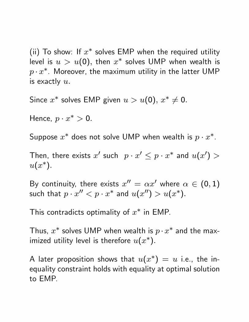
(ii) To show: If x∗ solves EMP when the required utilitylevel is u > u(0), then x∗ solves UMP when wealth isp ·x∗. Moreover, the maximum utility in the latter UMPis exactly u.

Since x∗ solves EMP given u > u(0), x∗ 6= 0.

Hence, p · x∗ > 0.

Suppose x∗ does not solve UMP when wealth is p · x∗.

Then, there exists x′ such p · x′ ≤ p · x∗ and u(x′) >u(x∗).

By continuity, there exists x′′ = αx′ where α ∈ (0, 1)such that p · x′′ < p · x∗ and u(x′′) > u(x∗).

This contradicts optimality of x∗ in EMP.

Thus, x∗ solves UMP when wealth is p ·x∗ and the max-imized utility level is therefore u(x∗).

A later proposition shows that u(x∗) = u i.e., the in-equality constraint holds with equality at optimal solutionto EMP.

Existence of solution to EMP: all we need is to ensurethat there exists x such that u(x) ≥ u.

Why?

The Expenditure Function: Given prices p � 0 and re-quired utility level u > u(0), the expenditure function isgiven by

e(p, u) = minx∈RL+

p · x

s.t. u(x) ≥ u.

Proposition 3.E.2: Suppose that u(.) is a continuous util-ity function representing a locally nonsatiated preferencerelation on X = RL+. The expenditure function e(p, u)

is:

(i) Homogenous of degree one in p.

(ii) Strictly increasing in u and nondecreasing in pl forany l

(iii) Concave in p

(iv) Continuos in p and u.

Implication of Proposition 3.E.1: Two identities: for anyp > 0, w > 0, u > u(0)

e(p, v(p, w)) = w

v(p, e(p, u)) = u

For a fixed price vector p = p,

e(p, u) = v−1(p, u)

v(p, w) = e−1(p, w)

Set of optimal solutions to EMP: h(p, u)

Called the Hicksian or compensated demand correspon-dence (or function if h(p, u) is single valued).

Proposition 3.E.3: Suppose that u(.) is a continuous util-ity function representing a locally nonsatiated preferencerelation on X = RL+. Then for any p � 0, u > u(0),

the Hicksian demand correspondence h(p, u) satisfies:

(i) Homogenous of degree zero in p : h(αp, u) = h(p, u)

for any α > 0

(ii) For any x ∈ h(p, u), u(x) = u.

(iii) Convexity/uniqueness: If % is convex so that u isquasiconcave, then h(p, u) is a convex set. If % is strictlyconvex so that u is strictly quasiconcave, then h(p, u)

consists of single point.

Suppose that u(.) is continuously differentiable.

Kuhn-Tucker first order necessary conditions: : If x∗ ∈h(p, u), then there exists a (scalar) multiplier λ ≥ 0 suchthat for all l = 1, ...L,

pl ≥ λ∂u(x∗)∂xl

and

pl = λ∂u(x∗)∂xl

if x∗l > 0.

Also,

u(x∗) = u.

The first set of conditions can be written as

p ≥ λ∇u(x∗)

and

x∗ · [p− λ∇u(x∗)] = 0.

If h(p, u) is single valued everywhere, then it is a contin-uous function.

First order conditions are suffi cient for optimality in theEMP if u is quasi-concave.

Implication of Proposition 3.E.1: Two more identities:for any p > 0, w > 0, u > u(0)

h(p, u) = x(p, e(p, u))

x(p, w) = h(p, v(p, w))

Note x(p, e(p, u)) is the Walrasian demand if for everyprice vector, wealth is adjusted to a level that allows theagent to just attain utility u.

This is the Hicksian compensation use to decompose ef-fect of price change into substitution and income effect.

The first identity therefore explains why h(p, u) is calledthe compensated demand.

Compensated Law of Demand

Modified Proposition 3.E.4: Suppose that u(.) is a con-tinuous utility function representing a locally nonsatiatedpreference relation on X = RL+. Then, for all p′, p′′ �0, u > u(0), x′ ∈ h(p′, u), x′′ ∈ h(p′′, u), the followingholds

(p′ − p′′)(x′ − x′′) ≤ 0.

Proof: As x′ ∈ h(p′, u), x′′ ∈ h(p′′, u)

p′x′ ≤ p′x′′

p′′x′′ ≤ p′′x′

and subtracting the second from the first inequality yieldsthe result.

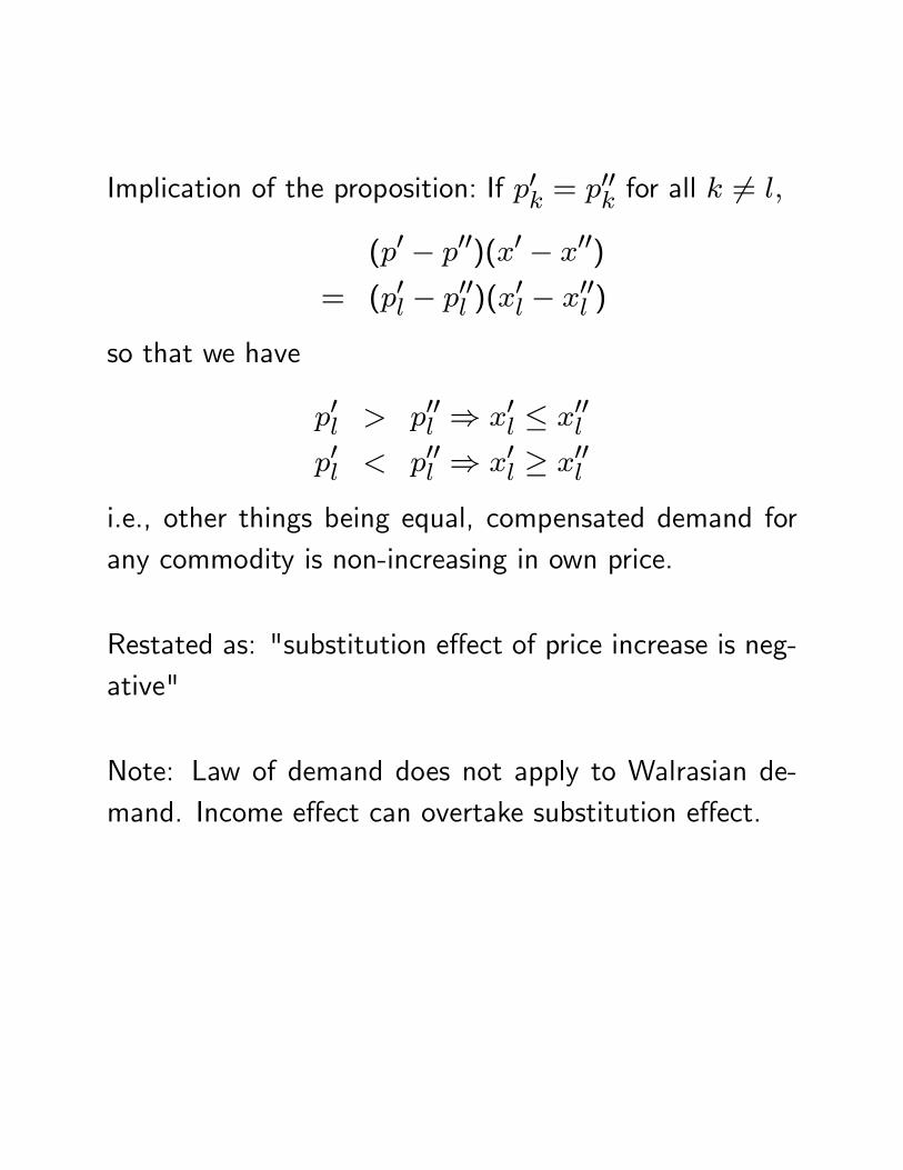
Implication of the proposition: If p′k = p′′k for all k 6= l,

(p′ − p′′)(x′ − x′′)= (p′l − p

′′l )(x′l − x

′′l )

so that we have

p′l > p′′l ⇒ x′l ≤ x′′l

p′l < p′′l ⇒ x′l ≥ x′′l

i.e., other things being equal, compensated demand forany commodity is non-increasing in own price.

Restated as: "substitution effect of price increase is neg-ative"

Note: Law of demand does not apply to Walrasian de-mand. Income effect can overtake substitution effect.

Some Useful Relationships between Demand, Indirect Util-ity and Expenditure Functions

Continue to assume: u(.) is a continuous utility functionrepresenting a locally nonsatiated preference relation onX = RL+.

Also, assume u is strictly quasi-concave.

Thus, x(p, w) and h(p, u) are single valued at each p�0, w > 0, u > u(0).

x(p, w) and h(p, u) are functions.

The maximum theorem can be used to show that thefunctions v(p, w), x(p, w), e(p, u) and h(p, u) are con-tinuos at every p� 0, w > 0, u > u(0).

Further, it can be shown that e(p, u) is differentiable atevery p� 0, u > u(0).

Proposition 3.G.1: At every p� 0, u > u(0),

hl(p, u) =∂e(p, u)

∂pl, l = 1, .., L.

"Proof": Easy to show under additional restriction thatthe utility function u is differentiable, h(p, u) is differen-tiable in p and h(p, u)� 0.

First order necessary condition for EMP: for some λ ≥ 0

(check λ is in fact > 0)

pk = λ∂u(h(p, u))

∂xk, k = 1, ...L.

Now,

u(h(p, u)) = u

As the latter is identity that holds for all p � 0, u >

u(0), we have by differentiating with respect to pl :

L∑k=1

∂u(h(p, u))

∂xk

∂hk(p, u)

∂pl= 0

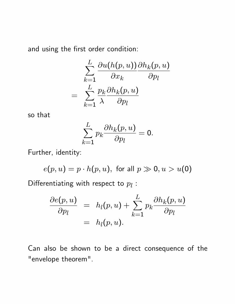
and using the first order condition:

L∑k=1

∂u(h(p, u))

∂xk

∂hk(p, u)

∂pl

=L∑k=1

pkλ

∂hk(p, u)

∂pl

so thatL∑k=1

pk∂hk(p, u)

∂pl= 0.

Further, identity:

e(p, u) = p · h(p, u), for all p� 0, u > u(0)

Differentiating with respect to pl :

∂e(p, u)

∂pl= hl(p, u) +

L∑k=1

pk∂hk(p, u)

∂pl

= hl(p, u).

Can also be shown to be a direct consequence of the"envelope theorem".

Implication.

Suppose that h(p, u) is continuously differentiable at (p, u).

Then, e(p, u) is twice continuously differentiable in p and

∂2e(p, u)

∂pk∂pl=∂hl(p, u)

∂pk.

Young’s theorem:

∂2e(p, u)

∂pk∂pl=∂2e(p, u)

∂pl∂pk

(for a twice continuously differentiable function, the sec-ond order partial derivatives are independent of the orderof differentiation).

For a twice differentiable concave function, the matrixof second order cross-partial derivatives (i.e., the Hessian

matrix) is negative semi-definite matrix.Thus,

∂2e∂p2

1

∂2e∂p1∂p2

∂2e∂p1∂pL

∂2e∂p2∂p1

∂2e∂p2

2

∂2e∂p2∂pL

∂2e∂pL∂p1

∂2e∂p2L

is a symmetric negative semi-definite matrix. This im-plies, the (Jacobian) matrix of first order derivatives ofh with respect to prices (i.e., the matrix of substitutioneffects)

∂h1∂p1

∂h2∂p1

∂hL∂p1

∂h1∂p2

∂h2∂p2

∂hL∂p2

∂h1∂pL

∂hL∂pL

is a symmetric negative semi-definite matrix. This matrixis sometimes called the substitution matrix.

As the diagonal terms of any negative semi-definite ma-trix is non-positive,

∂hl∂pl≤ 0, l = 1, ...L.

which the own price effect in the law of compensateddemand.

∂hl∂pk≥ 0 : goods l, k are substitutes

∂hl∂pk≤ 0 :goods l, k are complements

As h(p, u) is homogenous of degree zero in p, Euler’stheorem:

L∑k=1

∂hl∂pk

pk = 0, l = 1, ..., L.

As ∂hl∂pl≤ 0, ∂hl∂pk

≥ 0 for some k (every good has at leastone substitute).

Proposition 3.G.3: (Slutsky equation) For all p, w � 0

and u = v(p, w)

∂hl(p, u)

∂pk=∂xl(p, w)

∂pk+∂xl(p, w)

∂wxk(p, w) for all l, k

Proof. Choose any p, w � 0.Fix Let u = v(p, w). Then,e(p, u) = w. Identity in p:

hl(p, u) = xl(p, e(p, u))

Differentiating through with respect to pk and evaluatingat p, u :

∂hl(p, u)

∂pk=

∂xl(p, e(p, u))

∂pk+∂xl(p, e(p, u))

∂w

∂e(p, u)

∂pk

=∂xl(p, w)

∂pk+∂xl(p, w)

∂whk(p, u)

=∂xl(p, w)

∂pk+∂xl(p, w)

∂wxk(p, e(p, u))

=∂xl(p, w)

∂pk+∂xl(p, w)

∂wxk(p, w).

Implication: Effect of change of own price on Walrasiandemand

∂xl(p, w)

∂pl

=∂hl(p, u)

∂pl− ∂xl(p, w)

∂wxl(p, w)

= substitution effect + income effect

For a normal good, ∂xl(p,w)∂w ≥ 0, so that income and

substitution effects work in same direction (negative).

You can recover Walrasian demand function from the in-direct utility function.

Proposition 3.G.4. Suppose that the indirect utility func-tion v(p, w) is differentiable at p, w � 0.

xl(p, w) = −∂v(p, w)/∂pl∂v(p, w)/∂w

.

Proof. Choose any p, w � 0.Fix Let u = v(p, w). Then,e(p, u) = w.Identity in p:

v(p, e(p, u)) = u

Differentiating through with respect to pl and evaluatingat p = p :

∂v(p, e(p, u))

∂pl+∂v(p, e(p, u))

∂w

∂e(p, u)

∂pl= 0

so that

∂v(p, w)

∂pl+∂v(p, w)

∂whl(p, u) = 0

and as hl(p, u) = hl(p, v(p, w)) = xl(p, w), we have

∂v(p, w)

∂pl+∂v(p, w)

∂wxl(p, w) = 0

and this yields the result.

Welfare Evaluation of Economic Changes

Fix wealth w > 0.

Suppose that price vector changes from p0 to p1.

Consumer is better off as a result of this change if

∆v = v(p1, w)− v(p0, w) > 0

and worse off if the opposite is true. The specific amountof this change in welfare depends on the choice of utilityfunction (indirect utility function depends on u).

How then do we measure this welfare change?

Use money metric (indirect) utility.

Choose any utility function u, derive the indirect utilityfunction v. Now, choose any arbitrary price vector p� 0.

Consider the function

e(p, v(p, w)).

It is the (minimum) amount of money you need to spendat price vector p to attain same utility level as the max-imum utility you can attain where price vector is p andwealth is w. As e(p, v(p, w)) is strictly increasing in thesecond argument, it is nothing but a strictly increasingtransformation of the indirect utility function. So, thereis a utility function representing the same preference or-dering for which e(p, v(p, w)) is in fact the indirect utility(why?).

Also note that e(p, v(p, w)) does not depend on whichindirect utility v is chosen.

A dollar measure of the welfare change:

e(p, v(p1, w))− e(p, v(p0, w))

This measure is independent of which indirect utility v ischosen.

If we choose p = p0, we obtain a measure of welfarechange called Equivalent Variation (EV):

EV (p0, p1, w) = e(p0, v(p1, w))− e(p0, v(p0, w))

= e(p0, v(p1, w))− w

It is the dollar amount that the consume would be indif-ferent about accepting in lieu of the price change. Let

u0 = v(p0, w), u0 = v(p1, w),

Then,

EV (p0, p1, w) = e(p0, u1)− w

If we choose p = p1, we obtain a measure of welfarechange called Compensating Variation (CV):

CV (p0, p1, w) = e(p1, v(p1, w))− e(p1, v(p0, w))

= w − e(p1, u0)

It is the amount by which the agent must be compensatedafter a price change to make him as well off as before theprice change.

Both CV and EV can be interpreted as area to the left ofthe Hicksian demand curves.

Suppose p01 6= p1

1 and p0l = p1

l = pl for all l 6= 1.Letp−1 = (p2, ...pL).Then (assuming appropriate differen-tiability), as

h1(p, u) =∂e

∂p1,

EV (p0, p1, w) = e(p0, u1)− w= e(p0, u1)− e(p1, u1)

=∫ p0

1

p11

∂e(p1, p−1, u1)

∂p1dp1

=∫ p0

1

p11

h1(p1, p−1, u1)dp1.

Similarly,

CV (p0, p1, w) =∫ p0

1

p11

h1(p1, p−1, u0)dp1

Suppose good 1 is a normal good (income effect is strictlypositive). If p1

1 < p01 . In that case, for all p1 ∈ (p1

1, p01 ),

h1(p1, p−1, u1) > x1(p1, p−1, w) > h1(p1, p−1, u

0)

and

h1(p11, p−1, u

1) = x1(p11, p−1, w) > h1(p1

1, p−1, u0)

h1(p01, p−1, u

1) > x1(p01, p−1, w) = h1(p0

1, p−1, u0).

To see these inequalities, suppose that the agent is ini-tially facing prices vector p1 and enjoying utility u1.

If price of good 1 now increases to p1 > p11, then the

quantity bought will decline to h1(p1, p−1, u1) due to

substitution effect and then decline further to x1(p1, p−1, w)

due to income effect (as the good is a normal good) sothat h1(p1, p−1, u

1) > x1(p1, p−1, w) .

Next, suppose that the agent is initially facing prices vec-tor p0 and enjoying utility u0.

If price of good 1 now decreases to p1 < p01, then the

quantity bought will increase to h1(p1, p−1, u0) due to

substitution effect, and then increase further to x1(p1, p−1, w)

due to income effect (as the good is a normal good), sothat h1(p1, p−1, u

0) < x1(p1, p−1, w).

It follows therefore, that

EV (p0, p1, w)

=∫ p0

1

p11

h1(p1, p−1, u1)dp1

> CV (p0, p1, w)

=∫ p0

1

p11

h1(p1, p−1, u0)dp1.

It is easy to check that the same inequality holds if p11 >

p01 (keep in mind that the integrals equal to EV and CVare now negative numbers).

If good 1 is an inferior good, EV < CV.

If there is no income effect, EV = CV ; in particular, theHicksian and Walrasian demands coincide (as a functionof prices) and

EV (p0, p1, w) =∫ p0

1

p11

x1(p1, p−1, w)dp1 = CV (p0, p1, w)

i.e., as area to the left of the Walrasian demand curve forgood 1 (Marshallian consumer surplus).

This is what happens when the utility function is quasi-linear.

If the utility function is one where income effect is notzero then using the area to the left of the Walrasian de-mand curve can still be an approximation of CV or EVprovided price changes are very small.

Revealed Preference Approach to Law of Demand

(Samuelson)

Preferences are not observable, only choices are.

If choices made by individuals always satisfy some basicconsistency axioms, then we can obtain certain patternsof economic behavior including the law of demand.

Instead of imposing structures on unobservable prefer-ences, we need to think about what consistency require-ments on choices can generate.

Assume that for each (p, w), the consumer chooses aunique bundle x(p, w).[We say nothing about why theconsumer makes that choice.]

We call x(p, w) a demand function.

Further, assume x(p, w) is homogenous of degree zeroand satisfies Walras’law.

Weak Axiom of Revealed Preference (WARP): For anytwo price-wealth situations (p, w) and (p′, w′), the fol-lowing holds: if p · x(p′, w′) ≤ w and x(p′, w′) 6=x(p, w), then p′ · x(p, w) > w′.

Reasoning behind the axiom:

p · x(p′, w′) ≤ w and x(p′, w′) 6= x(p, w)

⇒ the bundle x(p′, w′) was affordable in the situationwhere consumer chose a different bundle x(p, w)

⇒ consumer revealed a preference for x(p, w) over x(p′, w′)

⇒ consumer should choose x(p, w) over x(p′, w′) when-ever both are affordable

⇒ since consumer chooses x(p′, w′) in situation (p′, w′),the bundle x(p, w) must not be affordable in this situa-tion

⇒ p′ · x(p, w) > w′.

Now, fix w and consider a price change from p to p′.

To remove income effect, adjust wealth to w′ so that atprice p′, the consumer can just afford the bundle x(p, w)

chosen prior to price change..

(Slutsky compensation criterion)

w′ = p′ · x(p, w)

Then, x(p′, w′) is the (Slutsky) compensated demand atprice p′.

(Proposition 2.F.1) Compensated Law of Demand.

If x(., .) satisfies homogeneity of degree zero, Walras’Law and WARP, then the following property holds:

for any compensated price change from a initial price-wealth situation (p, w) to a new situation (p′, w′) =

(p′, p′ · x(p, w)), we have

(p′ − p)[x(p′, w′)− x(p, w)] ≤ 0

with strict inequality whenever x(p, w) 6= x(p′, w′) i.e.,

Proof: The inequality is immediate if x(p, w) = x(p′, w′).So, suppose x(p, w) 6= x(p′, w′).

Then,

(p′ − p)[x(p′, w′)− x(p, w)]

= p′ · x(p′, w′)− p · x(p′, w′)− p′ · x(p, w) + p · x(p, w)

= w′ − p · x(p′, w′)− w′ + w,

using Walras Law and Slutsky compensation criterion,and the latter expression is

= w − p · x(p′, w′).

If w−p·x(p′, w′) ≥ 0, then WARP implies p′·x(p, w) >

w′ which violates the fact that w′ = p′ · x(p, w). Thus,

(p′ − p)[x(p′, w′)− x(p, w)]

= w − p · x(p′, w′) < 0.

This concludes the proof.