WWoorrkksshhoopp CCoouurrssee MMaatteerriiaall

1

Computer Aided Drug Design

Study Material

2

Contents:

S.No Topic: Page No:

1 Introduction to Computer Aided Drug

Design (CADD)

3

2 Importance of protein preparation 11

3 Define receptor region 13

4 Ligand Preparation 14

5 Molecular Docking 15

6 Binding Site Analysis 19

7 ADMET (Druggability Check) 20

8 Ligand Based Drug Design & QSAR 26

9 Homology Modelling 28

10 Cheminformatics Analysis 31

11 Biologics 39

12 Glossary 43

3

Introduction to Computer Aided Drug Design (CADD)

Discovery of new therapeutic solutions is an expensive and time-consuming process. It

is estimated that a typical drug discovery cycle, from lead identification through to

clinical trials can take more than 14 years (1). An emerging technology, Computer Aided

Drug Design (CADD) accelerates the drug development by making use of the

accumulated information of existing drugs and diseases, combined with inter-

disciplinary inputs from other fields. This technology extensively uses mathematical

models and simulation tools based on the evaluation of potential risks from drug safety

and the experimental design of new trials. The drug is most commonly an organic small

molecule which activates or inhibits the function of a biomolecule such as a protein

which in turn results in a therapeutic benefit to the patient. In the most basic sense,

drug design involves design of small molecules that are complementary in shape and

charge to the bimolecular target to which they interact and therefore will bind to it.

During the early 1980s, structural biologists began to design rational drugs based on

protein structures. The first projects were underway in the mid-1980s, and the first

successful stories, computer-aided rational design of peptide-based HIV-protease

inhibitors, were published by the early 1990s (2). Since then computational drug design

and discovery methods have traditionally put much importance on the identification of

novel active compounds and the optimization of their potency.

In CADD, computational tools and softwares are used to simulate drug receptor

interactions. Fast expansion in this area has been made possible by advances in

software and hardware computational power and sophistication, identification of

molecular targets, and an increasing database of publicly available target protein

structures. CADD is being utilized to identify hits (active drug candidates), select leads

(most likely candidates for further evaluation), and optimize leads i.e. transform

biologically active compounds into suitable drugs by improving their physicochemical,

pharmaceutical, ADMET/PK (pharmacokinetic) properties.

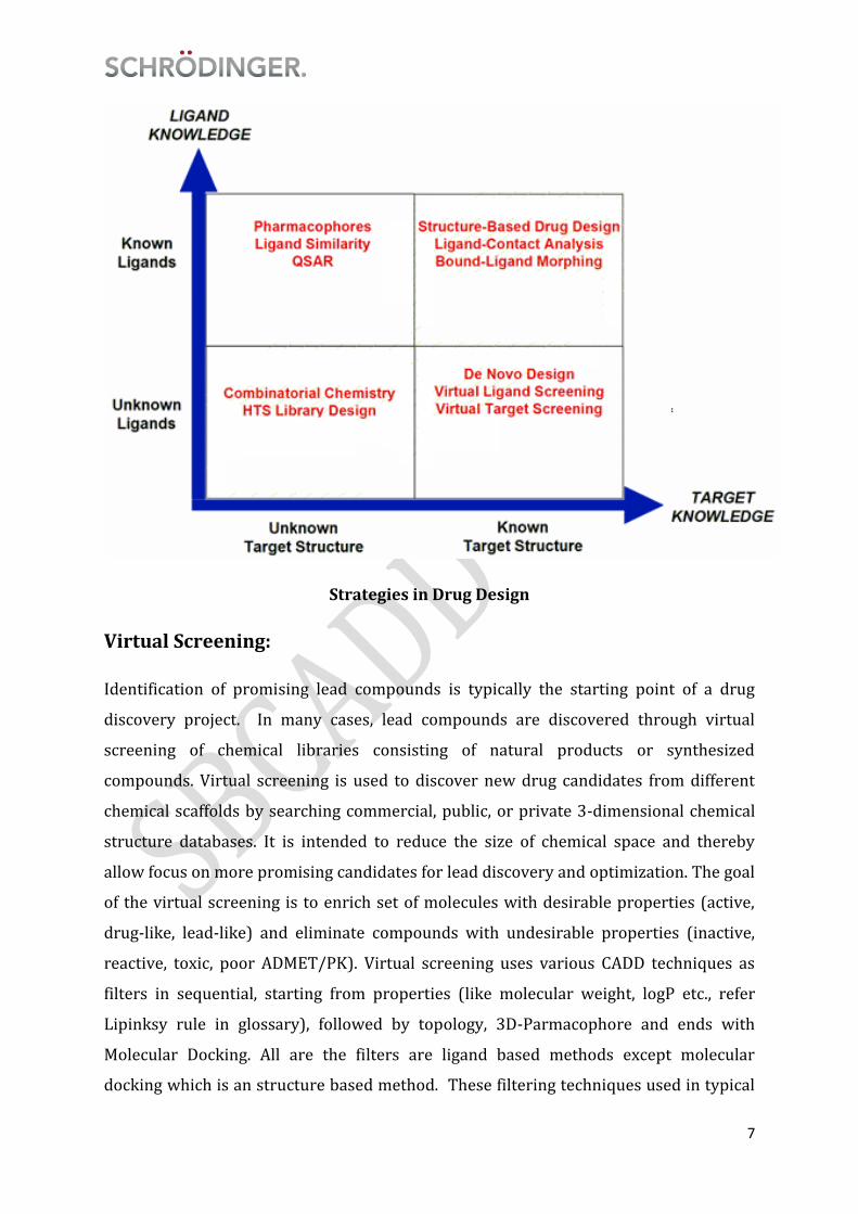
There are two major approaches in CADD:1) Structure based drug design and screening

2) Ligand based drug design and screening

4

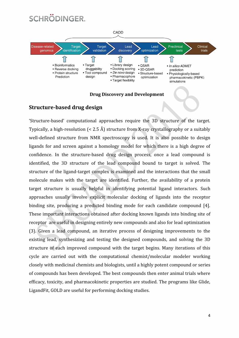
Drug Discovery and Development

Structure-based drug design

‘Structure-based’ computational approaches require the 3D structure of the target.

Typically, a high-resolution (< 2.5 Å) structure from X-ray crystallography or a suitably

well-defined structure from NMR spectroscopy is used. It is also possible to design

ligands for and screen against a homology model for which there is a high degree of

confidence. In the structure-based drug design process, once a lead compound is

identified, the 3D structure of the lead compound bound to target is solved. The

structure of the ligand-target complex is examined and the interactions that the small

molecule makes with the target are identified. Further, the availability of a protein

target structure is usually helpful in identifying potential ligand interactors. Such

approaches usually involve explicit molecular docking of ligands into the receptor

binding site, producing a predicted binding mode for each candidate compound [4].

These important interactions obtained after docking known ligands into binding site of

receptor are useful in designing entirely new compounds and also for lead optimization

(3). Given a lead compound, an iterative process of designing improvements to the

existing lead, synthesizing and testing the designed compounds, and solving the 3D

structure of each improved compound with the target begins. Many iterations of this

cycle are carried out with the computational chemist/molecular modeler working

closely with medicinal chemists and biologists, until a highly potent compound or series

of compounds has been developed. The best compounds then enter animal trials where

efficacy, toxicity, and pharmacokinetic properties are studied. The programs like Glide,

LigandFit, GOLD are useful for performing docking studies.

5

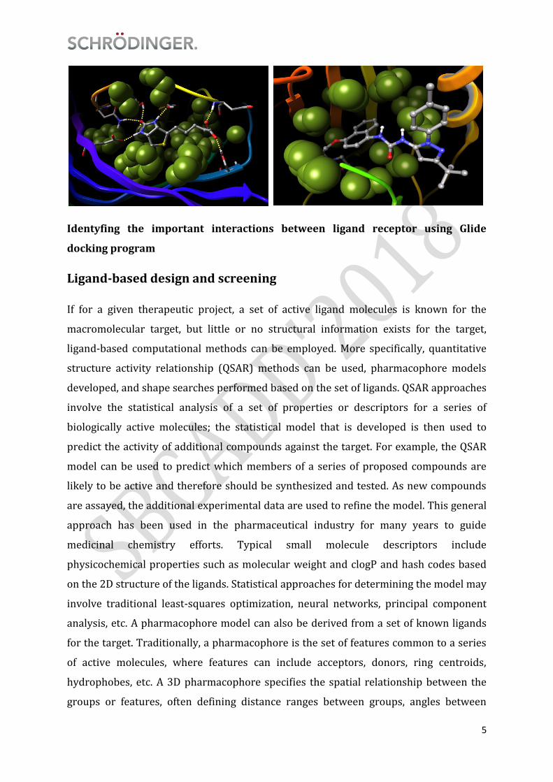
Identyfing the important interactions between ligand receptor using Glide

docking program

Ligand-based design and screening

If for a given therapeutic project, a set of active ligand molecules is known for the

macromolecular target, but little or no structural information exists for the target,

ligand-based computational methods can be employed. More specifically, quantitative

structure activity relationship (QSAR) methods can be used, pharmacophore models

developed, and shape searches performed based on the set of ligands. QSAR approaches

involve the statistical analysis of a set of properties or descriptors for a series of

biologically active molecules; the statistical model that is developed is then used to

predict the activity of additional compounds against the target. For example, the QSAR

model can be used to predict which members of a series of proposed compounds are

likely to be active and therefore should be synthesized and tested. As new compounds

are assayed, the additional experimental data are used to refine the model. This general

approach has been used in the pharmaceutical industry for many years to guide

medicinal chemistry efforts. Typical small molecule descriptors include

physicochemical properties such as molecular weight and clogP and hash codes based

on the 2D structure of the ligands. Statistical approaches for determining the model may

involve traditional least-squares optimization, neural networks, principal component

analysis, etc. A pharmacophore model can also be derived from a set of known ligands

for the target. Traditionally, a pharmacophore is the set of features common to a series

of active molecules, where features can include acceptors, donors, ring centroids,

hydrophobes, etc. A 3D pharmacophore specifies the spatial relationship between the

groups or features, often defining distance ranges between groups, angles between

6

groups or planes, and exclusion spheres. The programs like Phase, Catalyst and UNITY

can search large 2D or 3D molecular databases for additional molecules that possess the

pharmacophore (5). Given just one active ligand known to bind to the target, a shape

search can be performed, whereby 3D molecular databases are searched for other

compounds that have the same shape. Knowledge of the bound conformation of the

ligand is highly desirable and again can be obtained via NMR. If the bound ligand

structure is not known experimentally, the lowest energy conformation of the small

molecule in solution can be calculated and used for the shape search. With certain shape

search methods some chemical matching can also be specified in addition to shape fit.

3D molecular databases can then be searched for other compounds that fit into that

shape.

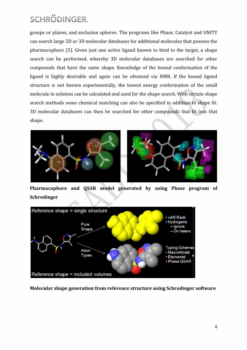
Pharmacophore and QSAR model generated by using Phase program of

Schrodinger

Molecular shape generation from reference structure using Schrodinger software

7

Strategies in Drug Design

Virtual Screening:

Identification of promising lead compounds is typically the starting point of a drug

discovery project. In many cases, lead compounds are discovered through virtual

screening of chemical libraries consisting of natural products or synthesized

compounds. Virtual screening is used to discover new drug candidates from different

chemical scaffolds by searching commercial, public, or private 3-dimensional chemical

structure databases. It is intended to reduce the size of chemical space and thereby

allow focus on more promising candidates for lead discovery and optimization. The goal

of the virtual screening is to enrich set of molecules with desirable properties (active,

drug-like, lead-like) and eliminate compounds with undesirable properties (inactive,

reactive, toxic, poor ADMET/PK). Virtual screening uses various CADD techniques as

filters in sequential, starting from properties (like molecular weight, logP etc., refer

Lipinksy rule in glossary), followed by topology, 3D-Parmacophore and ends with

Molecular Docking. All are the filters are ligand based methods except molecular

docking which is an structure based method. These filtering techniques used in typical

8

virtual screening protocol are illustrated. Thus virtual screening narrows down the

candidate compounds to be experimentally screened from millions to hundreds, leading

to an improved success rate of finding active compounds at a much lower cost. There

are several softwares available for performing ligand based virtual screening like Hip

Hop, Hypogen, Disco, Gaps, flo, APEX, and ROCS. For the structure based virtual

screening, Autodock, GOLD, FlexX, ICM, FRED and LigandFit etc are available. In

Schrodinger Software for performing structure based virtual screening, ‘Virtual

Screening Workflow’ is used and for ligand based studies, ‘Phase’and ‘Canvas’ are

used.

Virtual Screening Protocol

3D Filtering

o 3-point pharmacophores

o Distance

hashing

3D Fitting

o Flexible Docking

o From pre-computed

conformers

1D Filtering

o Property

Ranges

o Fingerprints

2D Filtering

o Topology, Molecular Graph

o (Red. Graphs, FTrees, …)

e.g. MW 200-500

Lipinsky

9

Chemical Libraries for virtual screening:

The National Cancer Institute (NCI) provides calculated structures for about 540,000 of

its compounds, and will provide at least some of these for experimental testing

(http://cactus.nci.nih.gov/). MDL Inc. sells the Available Chemicals Directory (ACD;

http://www.mdl.com/products/experiment/available_chem_dir/index.jsp) of

commercially available compounds and the ACD-SC for screening collections. To use

these libraries in docking screens, molecular properties such as protonation, charge,

stereochemistry, accessible conformations and solvation must be calculated. Recently,

about one million commercially accessible molecules have become available through

the ZINC database (http://blaster.docking.org/zinc/). ZINC is a free. CSD is another

database which contains crystal structures of small molecules. Other databases like

Asinex, May-Bridge and world drug index (WDI) contains millions of compounds

available for virtual screening.

Success Stories of CADD:

Numerous successes of designed drugs were reported, including Dorzolamide for the

treatment of cystoid macular edema [6], Zanamivir for therapeutic or prophylactic

treatment of influenza infection [7], Sildenafil for the treatment of male erectile

dysfunction [8], and Amprenavir for the treatment of HIV infection [9]

Present and future

Today, computer-aided drug design and screening methods impact the efforts of all

pharmaceutical companies. As the computational technologies advance, the role they

play in improving the efficiency of the drug discovery process will become increasingly

important. In addition, as the body of structural information on potential therapeutic

targets dramatically expands, which is expected to happen in the next few years, it will

drive the development of the computational methodology. Greater automation, faster

algorithms, and improved information management techniques will be required to

handle the sheer volume of target-related information that will need to be processed.

On a genomic scale, instead of looking at individual targets, families of related targets

will be studied. The information available on ligand binding to these families will be

10

vastly expanded. The job of the molecular modeler will be to effectively mine this data

as well as translate the available structural information into a form directly usable by

the bench chemist. This mission will ultimately cause a greater interface of bio- and

chemoinformatics, leading to improved structural and functional genomics knowledge.

References:

1. Myers S, Baker A. Drug discovery—an operating model for a new era. Nat Biotechnol

2001;19:727–30

2. Erickson, J.; Neidhart, D.J.; VanDrie, J.; Kempf, D.J.; Wang, X.C.; Norbeck, D.W.; Plattner,

J.J.; Rittenhouse, J.W.; Turon, M.;Wideburg, N. Science, 1990, 249, 527-533

3. Kuntz, I.D. Science, 1992, 257, 1078-1082

4. Lyne PD. Structure-based virtual screening: an overview. DrugDiscovToday

2002;7:1047–55

5. J Med Chem 2005;48(20):6250–6260. [PubMed:16190752]

6. Grover S, Apushkin MA, Fishman GA. Am JOphthalmol 2006;141:850–8

7 . Von Itzstein M, Wu WY, Kok GB, et al Nature 1993;363:418–23

8 .Terrett NK, Bell AS, Brown D, et al BioorgMed Chem Lett 1996;6:1819–24

9. Goodgame JC, Pottage JC Jr, Jablonowski H, et al, Antivir Ther 2000;5:215–25.

11

Importance of protein preparation

The quality of any docking results depends on reasonable starting structures for both

the protein and the ligand. It is strongly recommended that you process protein and

ligand structures with these facilities in order to achieve the best results.

Protein and preparation:

A typical PDB structure file consists only of heavy atoms, can contain waters,

cofactors, and metal ions, and can be multimeric. The structure generally has no

information on bond orders, topologies, or formal atomic charges. Terminal amide

groups can also be misaligned, because the X-ray structure analysis cannot usually

distinguish between O and NH2. Ionization and tautomeric states are also generally

unassigned. Most of the docking programs requires bond orders and ionization states to

be properly assigned and performs better when side chains are reoriented when

necessary and steric clashes are relieved.

The water molecules present in the PDB structure are identified by the oxygen

atom, and usually do not have hydrogens attached. Generally, all waters (except those

coordinated to metals) are deleted, but waters that bridge between the ligand and the

protein are sometimes retained. If waters are kept, hydrogens will be added to them.

The atom types for metal ions are sometimes incorrectly translated into dummy atom

types when metal-protein bonds are specified in the input structure. It may be

necessary to adjust the protonation of the protein, which is crucial when the receptor

site is a metalloprotein such as thermolysin or an MMP. Finally the protein should be

minimized to reorient side-chain hydroxyl groups and alleviate potential steric clashes

present in the PDB structure

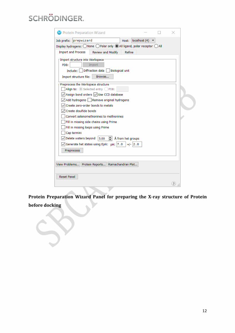
Schrödinger offers a comprehensive protein preparation facility in the Protein

Preparation Wizard, which is designed to ensure chemical correctness and to optimize

protein, the layout of the panel is shown in the figure below:

12

Protein Preparation Wizard Panel for preparing the X-ray structure of Protein

before docking

13

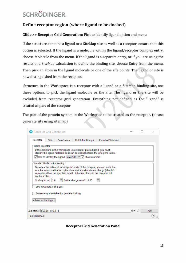
Define receptor region (where ligand to be docked)

Glide >> Receptor Grid Generation: Pick to identify ligand option and menu

If the structure contains a ligand or a SiteMap site as well as a receptor, ensure that this

option is selected. If the ligand is a molecule within the ligand/receptor complex entry,

choose Molecule from the menu. If the ligand is a separate entry, or if you are using the

results of a SiteMap calculation to define the binding site, choose Entry from the menu.

Then pick an atom in the ligand molecule or one of the site points. The ligand or site is

now distinguished from the receptor.

Structure in the Workspace is a receptor with a ligand or a SiteMap binding site, use

these options to pick the ligand molecule or the site. The ligand or the site will be

excluded from receptor grid generation. Everything not defined as the "ligand" is

treated as part of the receptor.

The part of the protein system in the Workspace to be treated as the receptor. (please

generate site using sitemap)

Receptor Grid Generation Panel

14

Ligand Preparation:

To give the best results, the structures that are docked must be good representations of

the actual ligand structures as they would appear in a protein-ligand complex. Most of

the docking tools only modify the torsional internal coordinates of the ligand during

docking, so the rest of the geometric parameters must be optimized beforehand. This

means that the structures supplied to docking tool must meet the following conditions:

1. They must be three-dimensional (3D)

2. They must have realistic bond lengths and bond angles.

3. They must each consist of a single molecule that has no covalent bonds to the

receptor, with no accompanying fragments, such as counter ions and solvent molecules.

4. They must have all their hydrogens (filled valences).

5. They must have an appropriate protonation state for physiological pH values

Schrödinger offers the ligand preparation facility in LigPrep. All of the above conditions

can be met by using LigPrep to prepare the structures. The LigPrep process consists of a

series of steps that perform conversions, apply corrections to the structures, generate

variations on the structures, eliminate unwanted structures, and optimize the

structures. The layout of ligand preparation panel (ligprep) is shown in the figure

below.

Ligprep panel for ligand preparation

15

Molecular Docking

Docking procedures aim to identify correct poses of ligands in the binding pocket of a

protein and to predict the affinity between the ligand and the protein. In other words,

docking describes a process by which two molecules fit together in three-dimensional

space.

Basic Requirements for Molecular Docking

The setup for a ligand docking approach requires the following components: A target

protein structure with or without a bound ligand, the molecules of interest or a

database containing existing or virtual compounds for the docking process, and a

computational framework that allows the implementation of the desired docking and

scoring procedures. The three-dimensional structure of the protein ligand complex has

to be detailed at atomic resolution. In many cases only the unbound (ligand-free, apo)

form of the protein is determined, without the bioactive conformation of the ligand.

Most docking algorithms assume the protein to be rigid, according to the high

computational cost that the demand of flexibility implicates. The ligand is mostly

regarded as flexible. Beside the conformational degrees of freedom the binding pose in

the protein's binding pocket must be taken into consideration. Docking can be

performed by placing rigid molecules or fragments into the protein's active site using

different approaches like the clique-search, geometric hashing, or pose clustering. The

flexibility of the ligand can be represented by a set of conformers covering the

conformational space in an exhaustive way.

SCORING METHODS

Scoring of docked poses is still regarded as one of the major challenges in the field of

molecular docking. The purpose of the scoring procedure is the identification of the

correct binding pose by its lowest energy value, and the ranking of protein-ligand

complexes according to their binding affinities. Scoring functions can be divided in

empirical scoring functions, scoring functions derived from force fields, and knowledge-

based scoring functions. Scoring functions derived from force fields handle the ligand

binding prediction with the use of potential energies (non-bonded interaction terms)

and sometimes in combination with solvations and entropy contributions. Knowledge-

based scoring functions are based on atom pair potentials derived from structural

16

databases. Forces and potentials are collected from known protein-ligand complexes to

get a score for their binding affinities (e.g. PMF). Empirical scoring functions derive

from training sets of protein-ligand complexes with determined affinity data. One

general aspect in the finding of an accurate empirical scoring function is the assumption

that each occurrence of an individual interaction is considered as equivalent.

Schrödinger implements docking using Glide (Grid-based Ligand Docking with

Energetics). Glide searches for favorable interactions between one or more ligand

molecules and a receptor molecule, usually a protein. Each ligand must be a single

molecule, while the receptor may include more than one molecule, e.g., a protein and a

cofactor. Glide can be run in rigid or flexible docking modes; the latter automatically

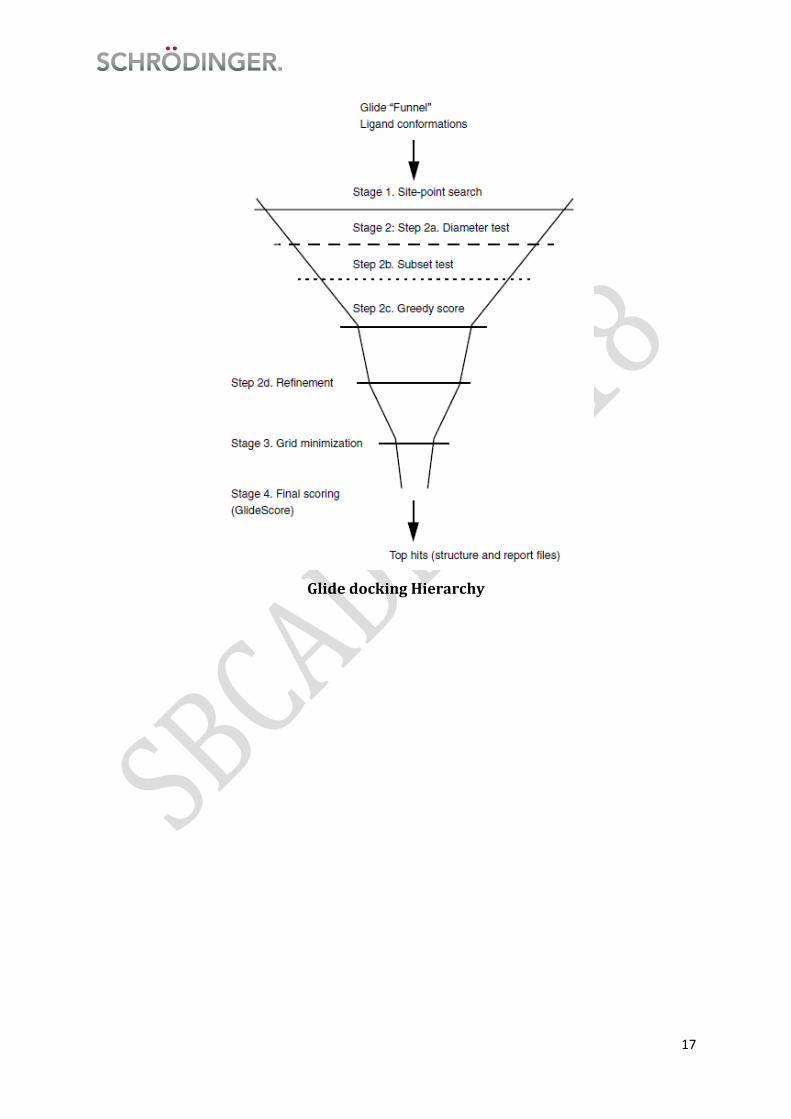
generates conformations for each input ligand. The ligand poses that Glide generates

pass through a series of hierarchical filters that evaluate the ligand’s interaction with

the receptor. The initial filters test the spatial fit of the ligand to the defined active site,

and examine the complementarity of ligand-receptor interactions using a grid-based

method patterned after the empirical ChemScore function. Poses that pass these initial

screens enter the final stage of the algorithm, which involves evaluation and

minimization of a grid approximation to the OPLS-AA nonbonded ligand-receptor

interaction energy. Final scoring is then carried out on the energy-minimized poses. By

default, Schrödinger’s proprietary GlideScore multi-ligand scoring function is used to

score the poses. If GlideScore was selected as the scoring function, a composite Emodel

score is then used to rank the poses of each ligand and to select the poses to be reported

to the user. Emodel combines GlideScore, the nonbonded interaction energy, and, for

flexible docking, the excess internal energy of the generated ligand conformation.

17

Glide docking Hierarchy

18

Glide Docking panel

19

Binding Site Analysis

Understanding the structure and function of protein binding sites is a cornerstone of

structure-based drug design. Developing this understanding requires knowledge of both

the location and physical properties of the binding site. In addition, the identification of

small-molecule binding sites as modulators of protein-protein interactions is of

increasing interest. Furthermore, even when a validated binding site has been

identified, it is often important to find additional potential binding sites where

appropriate targeting could result in different biological effects or new classes of

compounds. When the binding site is not known from a 3-D structure or from other

experimental data, computational methods can be employed to suggest likely locations.

When the location of the primary binding site is known, medicinal chemistry efforts to

design better ligands can profit from a better understanding of the degree to which

known ligands are, or fail to be, complementary to the receptor as well as from a critical

assessment of the degree to which the occupancy of accessible but unexplored regions

by appropriate ligand functionality can be expected to promote binding or could be

used to improve the physical properties of the ligand without lessening its binding

affinity. Such assessments can assist in the evaluation and optimization both of known

binding molecules and of virtual screening hits. It is also important to understand the

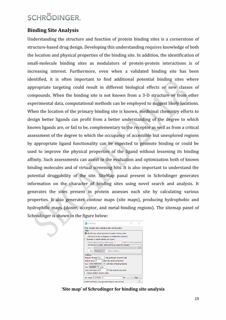
potential druggability of the site. SiteMap panal present in Schrödinger generates

information on the character of binding sites using novel search and analysis. It

generates the sites present in protein assesses each site by calculating various

properties. It also generates contour maps (site maps), producing hydrophobic and

hydrophilic maps (donor, acceptor, and metal-binding regions). The sitemap panel of

Schrodinger is shown in the figure below:

‘Site map’ of Schrodinger for binding site analysis

20

ADMET (Druggability Check)

Drug discovery and development are expensive and time-consuming processes.

Recognition by the pharmaceutical industry that undesirable absorption, distribution,

metabolism and excretion (ADME) properties of new drug candidates are the cause of

many clinical phase drug development failures has resulted in a paradigm shift to

identify such problems early in the drug discovery process Thus, in vitro approaches are

now widely used to investigate the ADME properties of new chemical entities and, more

recently, computational (in silico) modelling has been investigated as a tool to optimise

selection of the most suitable drug candidates for development. The objectives of in

silico modeling tools for predicting these properties to serve two key aims — first, at

the design stage of new compounds and compound libraries so as to reduce the risk of

late-stage attrition; and second, to optimize the screening and testing bylooking at only

the most promising compounds.

Drug-like properties. The properties which can differentiate drugs from other chemicals

can be considered as drug like properties. The crucial properties that should be

considered for compounds with oral delivery (Lipinski’s ‘rule-of-five’) includes

molecular mass <500 Daltons (Da), calculated octanol/water partition coefficient

(CLOGP) <5, number of hydrogen-bond donors <5 and number of hydrogen-bond

acceptors <10. These properties are then typically used to construct predictive ADME

models and form the basis for what has been called property-based design.

What ADME properties do we want to predict?

A deeper understanding of the relationships between important ADME parameters and

molecular structure and properties has been used to develop in silico models that allow

the early estimation of several ADME properties. Among other important issues, we

want to predict properties that provide information about dose size and dose frequency

such as oral absorption, bioavailability, brain penetration, clearance (for exposure) and

volume of distribution (for frequency). As a result of the availability of experimental

data in the literature, considerable effort has gone into the development of models to

predict physicochemical properties relevant to ADME, such as lipophilicity. However,

despite its importance, the prediction of pharmacokinetic properties such as clearance,

volume of distribution and half-life directly from molecular structure is making slower

21

progress owing to a lack of published data. Similarly, the prediction of various aspects of

metabolism and toxicity is also underdeveloped.

Prediction of ADME and related properties

Absorption. For a compound crossing a membrane by purely passive diffusion, a

reasonable permeability estimate can be made using single molecular properties, such

as log D or hydrogen-bonding capacity. The simplest insilico models for estimating

absorption are based on a single descriptor, such as log P or log D, or polar surface area,

which is a descriptor of hydrogen-bonding potential. Different multivariate approaches,

such as multiple linear regressions, partial least squares and artificial neural networks,

have been used to develop quantitative structure–human-intestinal-absorption

relationships.

Bioavailability. Important properties for determining permeability seem to be the size

of the molecule, as well as its capacity to make hydrogen bonds, its overall lipophilicity

and possibly its shape and flexibility.

Blood–brain barrier penetration. Drugs that act in the CNS need to cross the blood–

brain barrier (BBB) to reach their molecular target. By contrast, for drugs with a

peripheral target, little or no BBB penetration might be required in order to avoid CNS

side effects. ‘Rule-of-five’-like recommendations regarding the molecular parameters

that contribute to the ability of molecules to cross the BBB have been made to aid BBB-

penetration predictions; for example, molecules with a molecular mass of <450 Da or

with PSA <100 Å2 are more likely to penetrate the BBB.

Dermal and ocular penetration. The existing transdermal models are typically a function

of the octanol/water partition coefficient and terms that have been associated with

aqueous solubility, including hydrogen-bonding parameters,molecular weight and

molecular flexibility. Commercial models for the prediction of solute-permeation rates

through the skin are available, for example, the QikProp and DermWin programs.

Metabolism. In silico approaches to predicting metabolism can be divided into QSAR

and three-dimensional- QSAR studies, protein and pharmacophore models and

predictive databases. Some of the first-generation predictive-metabolism tools

currently require considerable input from a computational chemist, whereas others can

22

be used as rapid filters for the screening of virtual libraries, for example, to test for

CYP3A4 liability. Perhaps the most intellectually satisfying molecular modeling studies

are those based on the crystal structure of the metabolizing enzymes several

approaches that use databases to predict metabolism are available. Ultimately, such

programs might be linked to computer-aided toxicity prediction on the basis of

quantitative structure–toxicity relationships and expert systems for toxicity evaluation

In silico prediction of toxicity issues

Toxicity is responsible for many compounds failing to reach the market and for the

withdrawal of a significant number of compounds from the market once they have been

approved. It has been estimated that ~20–40% of drug failures in investigational drug

development can be attributed to toxicity concerns. The existing commercially available

in silico tools for forecasting potential toxicity issues can be roughly classified into two

groups. The first approach uses expert systems that derive models on the basis of

abstracting and codifying knowledge from human experts and the scientific literature.

The second approach relies primarily on the generation of descriptors of chemical

structure and statistical analysis of the relationships between these descriptors and the

toxicological end-point.

QikProp is a quick, accurate, easy-to-use absorption, distribution, metabolism, and

excretion (ADME) prediction program present in the Schrödinger suite. QikProp

predicts physically significant descriptors and pharmaceutically relevant properties of

organic molecules, either individually or in batches. In addition to predicting molecular

properties, QikProp provides ranges for comparing a particular molecule’s properties

with those of 95% of known drugs. QikProp also flags 30 types of reactive functional

groups that may cause false positives in high-throughput screening (HTS) assays.

Outlay of Qikprop panel for ADME prediction

23

Ligand Based Drug Design (Phase & QSAR)

Pharmacophore Modeling

The official 1998 IUPAC definition 1 is as follows: “A pharmacophore is the ensemble of

steric and electronic features that is necessary to ensure the optimal supramolecular

interactions with a specific biological target structure and to trigger (or to block) its

biological response.”

A pharmacophore does not represent a real molecule or a real association of

functional groups, but a purely abstract concept that accounts for the common

molecular interaction capacities of a group of compounds towards their target

structure. The pharmacophore can be considered as the largest common denominator

shared by a set of active molecules.

Central to the pharmacophore concept is the notion that the molecular

recognition of a biological target shared by a group of compounds can be ascribed to a

(small) set of common features that interact with a set of complementary sites on the

biological target. In pharmacophore research quite general features such as hydrogen-

bond donors, hydrogen-bond acceptors, positively and negatively charged groups, and

hydrophobic regions are typically used. The other key component of contemporary

pharmacophore research is the incorporation of information about the three-

dimensional nature of molecular interactions. The focus of this perspective is on

3Dpharmacophore methods in which the spatial relationship between the

pharmacophore features is also specified

Pharmacophore Elucidation:

Pharmacophore elucidation is a molecular alignment problem, the aim being to

superimpose a set of active ligands, all of which bind to the same protein of unknown

3D structure, so that the features they have in common become evident. A number of

programs for pharmacophore elucidation are widely used largely because of their

availability in commercial software packages. These include CATALYST,16 GALAHAD,

17 GASP,18 the pharmacophore module of MOE,19 and PHASE.20 All pharmacophore

elucidation algorithms must include methods for (a) representing the ligands (i.e.,

placing points on or around the molecules to represent the various pharmacophoric

features they contain), (b) searching for candidate alignments, (c) scoring those

alignments. These aspects are considered separately. Three main stages can be

24

identified in the elucidation of a pharmacophore. First, prepare the data set. Second,

generate possible pharmacophores. Third, validate the pharmacophore(s).

3D Database Searching

One of the common purposes of making pharmacophore models is to search for novel

chemical matter. The pharmacophore represents an abstraction that can be used to find

alternative chemotypes (i.e., chemical series with a different underlying framework,

scaffold, or common moiety). Depending on the precision of the query, one can find

numbers of hits from 10s to 1000s, which was in line with the screening capacities

available at the time. Many will be false positives and show no activity in the screen, but

generally, the hit rates from pharmacophore searches are much higher than from

random screening. The hits can also sample very novel and diverse chemotypes,

allowing the medicinal chemist the luxury of pursuing the series with the best overall

profile.

In Schrödinger, pharmacophore studies are implemented in Phase. Phase is a versatile

product for pharmacophore perception, structure alignment, activity prediction, and 3D

database searching. Given a set of molecules with high affinity for a particular protein

target, Phase uses fine-grained conformational sampling and a range of scoring

techniques to identify common pharmacophore hypotheses, which convey

characteristics of 3D chemical structures that are purported to be critical for binding.

Each hypothesis is accompanied by a set of aligned conformations that suggest the

relative manner in which the molecules are likely to bind.

Phase consists of the following four workflows:

Building a pharmacophore model (and an optional QSAR models) from a set of

ligands

Pharmacophore feature generation from single molecule

Optimal Pharmacophore features from receptor ligand complex

Pharmacophore features from receptor binding cavity or from protein residues

Building a pharmacophore hypothesis from a single ligand (and editing it)

Preparing a 3D database that includes pharmacophore information

Searching the database for matches to a pharmacophore hypothesis

25

Phase-Develop pharmacophore panel for pharmacophore and QSAR studies

QSAR (Quantitative Structural Activity Relationship)

26

QSAR is a method used to find relationship between physicochemical properties of

chemical substances and their biological activities.

Find a mathematical formula (using regression techniques) which relates the biological

property/activity of a series of compounds to their physicochemical/structural

parameters. Starting with a set of compounds with known biological property, the set is

divided into train and test subsets. The mathematical formula is derived from the train

set using the known biological activity and physicochemical properties. The formula (or

model) is validated by applying it on the test set compounds. This formula or model,

provided it shows good performance during validation, is then used to predict the

biological property of new/novel compounds.

Fundamental principle: difference in structural properties is responsible for the

variations in biological activities of the compounds

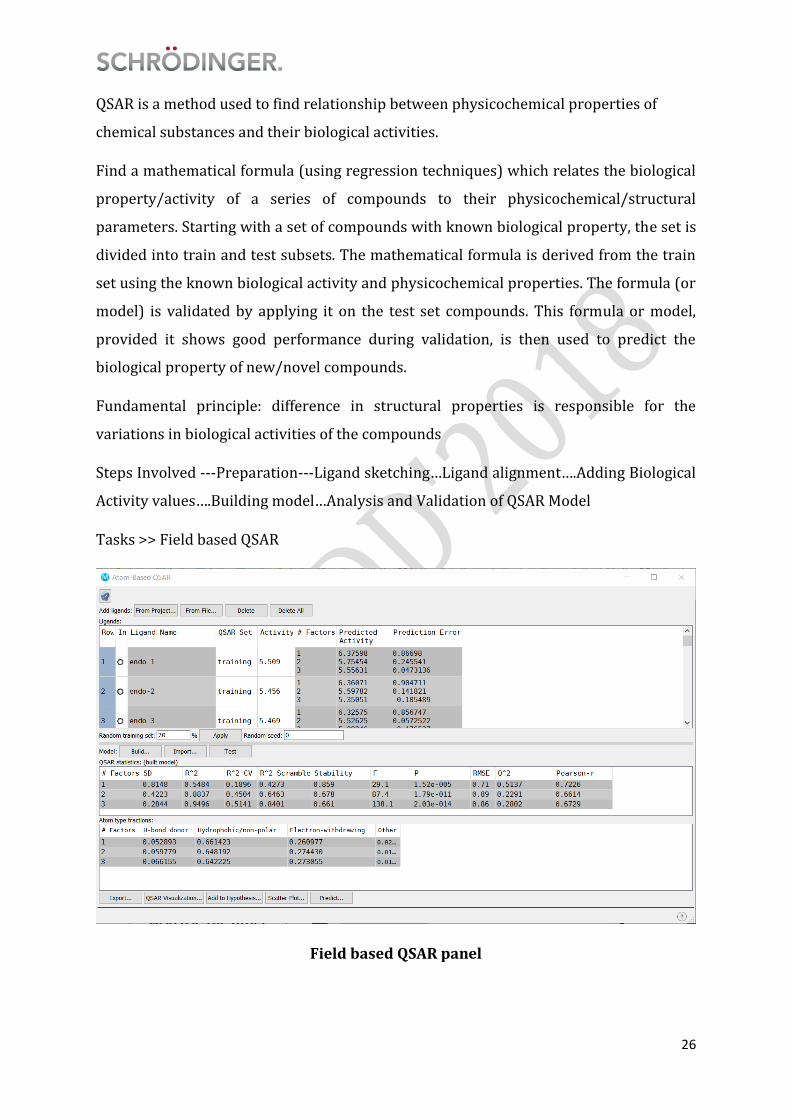
Steps Involved ---Preparation---Ligand sketching…Ligand alignment….Adding Biological

Activity values….Building model…Analysis and Validation of QSAR Model

Tasks >> Field based QSAR

Field based QSAR panel

27

QSAR contour maps

28

Homology Modeling:

With the development of techniques in molecular biology that allow rapid identification,

isolation, and sequencing of genes, we are now able to infer the sequences of many

proteins. However, it is still a time-consuming task to obtain the three-dimensional

structures of these proteins. A major goal of structural biology is to predict the three-

dimensional structure from the sequence, a pursuit that has not yet been realized. Thus,

alternative strategies are being applied to develop models of protein structure when the

constraints from X-ray diffraction or NMR are not yet available.

One method that can be applied to generate reasonable models of protein structures is

homology modeling. This procedure, also termed comparative modeling or knowledge-

based modeling, develops a three-dimensional model from a protein sequence based on

the structures of homologous proteins. In the description that follows, some aspects of

homology modeling that you may find useful in this course and in your research are

discussed.

What is Homology?

Care must be used in applying the term, "homology modeling." In fact, as noted above

some authors prefer alternative names for the procedure. One must recognize that

homology does not necessarily imply similarity. Homology has a precise definition:

having a common evolutionary origin. Thus, homology is a qualitative description of the

nature of the relationship between two or more things, and it cannot be partial. Either

there is an evolutionary relationship or there is not. An assertion of homology usually

must remain an hypothesis. Supporting data for a homologous relationship may include

sequence or three-dimensional similarities, the relationships between which can be

described in quantitative terms.

An observation of importance in homology modeling is that for a set of proteins that are

hypothesized to be homologous, their three-dimensional structures are conserved to a

greater extent than are their primary structures. This observation has been used to

generate models of proteins from homologues with very low sequence similarities.

Thus, in homology modeling, we are attempting to develop models of an unknown from

29

homologous proteins. These proteins will have some measure of sequence similarity but

we are relying on the conservation of folds among homologues to guide us as well.

The steps to creating a homology model are as follows:

1. identify homologous proteins and determine the extent of their sequence

similarity with one another and the unknown

2. align the sequences

3. identify structurally conserved and structurally variable regions

4. generate coordinates for core (structurally conserved) residues of the unknown

structure from those of the known structure(s)

5. generate conformations for the loops (structurally variable) in the unknown

structure

6. build the side-chain conformations

7. refine and evaluate the unknown structure.

Prime 3.0 is a highly accurate protein structure prediction suite of programs that

integrates Comparative Modeling and Fold Recognition into a single user-friendly,

wizard-like interface. The Comparative Modeling path incorporates the complete

protein structure prediction process from template identification, to alignment, to

model building. Refinement can then be done from a separate panel, and involves side-

chain prediction, loop prediction, and minimization. The Prime interface was designed

to accommodate both novice and expert users, while the underlying programs were

designed to produce superior results in a variety of applications, including:

• High-resolution homology modeling

• Refinement of active sites

• Induced-fit optimization

• Fold Recognition

• Structure-based functional annotation

• Generation of alternate loop conformations

30

Prime and homology modeling panel of Schrödinger

31

Cheminformatics Analysis

Projects in Canvas

We will use Canvas to open a pre-generated project, and save it as a new project.

1. Double-click the Canvas icon

○ (No icon? See Starting

Canvas)

2. In the Canvas toolbar, click

Open Project

3. Navigate to CDK_dataset.cnvzip

4. Select the file and click Open

Project

○ The viewer contains a

dataset of CDK

inhibitors with Structure

and Affinity value fields

The Canvas User Interface with the

CDK dataset loaded

5. This project is in the form of a

Scratch Project which can be

saved under a new name and

re-saved

6. File > Save Project as

7. In File Name, type

CDK_dataset.cnv and click Save

○ The project is saved as

CDK_dataset.cnv

Note: Canvas projects are laid out by:

- Rows and Columns of data form

the majority of the Project View

- All Applications and their job

32

status in a list on the right hand

side of this GUI

- The lower part of the window

houses the log file of the

running job

- Useful icons are located along

the top of the Panel

33

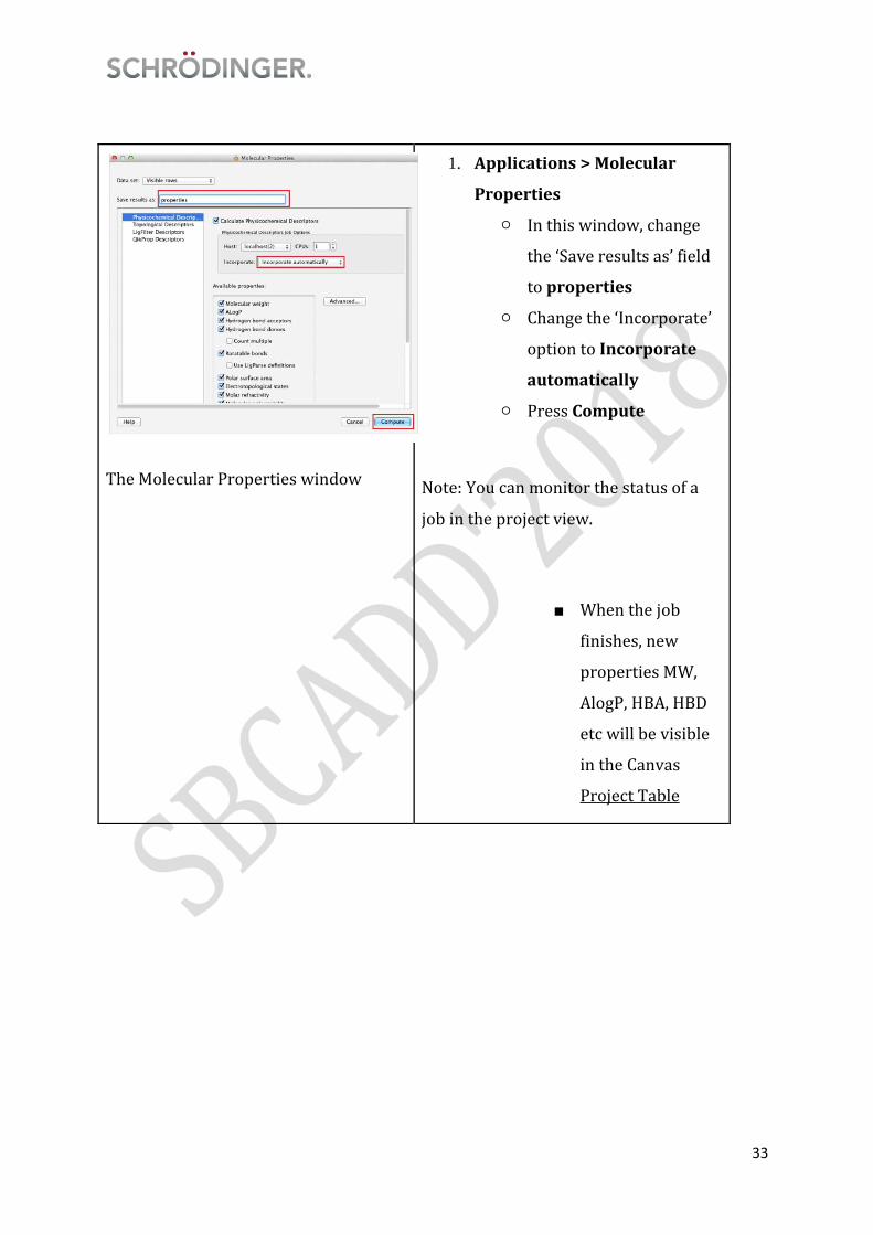
The Molecular Properties window

1. Applications > Molecular

Properties

○ In this window, change

the ‘Save results as’ field

to properties

○ Change the ‘Incorporate’

option to Incorporate

automatically

○ Press Compute

Note: You can monitor the status of a

job in the project view.

■ When the job

finishes, new

properties MW,

AlogP, HBA, HBD

etc will be visible

in the Canvas

Project Table

34

Here, we generate the Linear and Radial fingerprints for the entire dataset in the Binary

Fingerprint panel.

Open the Binary Fingerprint panel and in the first instance, keep all the default settings

for generating Linear Fingerprints

The binary fingerprint panel.

1. On the left, navigate to

Applications > Binary

Fingerprints

2. Press Create to generate linear

fingerprints

3. Choose incorporate

automatically

4. Click OK

5. When the job finishes, navigate

to Applications > Radial (ECFP)

○ Two fingerprint fields

titled fp_linear_1 and

fp_radial_2 are in in the

Project Table

The CDK dataset with calculated

properties

Note: Changes in the right hand side

panel – Under the Descriptors heading,

a sub field showing the job is now

visible as ‘properties’ and along with

its job status as ‘Incorporated’ ; you can

right-click on this to see other options

but do not select them

35

Note: The Advanced options below the

Fingerprints list, houses the atom-

typing information. This is automatically

set to the ideal atom-typing for the

fingerprint chosen in the main panel. If

click through different options of

Fingerprints, the atom-typing changes

as a result.

The Heatmap panel

1. Data > Heat Map

2. In the Properties group, ctrl-

click (cmd-click) AlogP,

HBA, HBD, and Affinity

cdk2 (uM)

3. Click Add

Note: Adjust the colors representing

Minimum and Maximum values by

right-clicking the colored boxes for

more choice.

36

Visualizing Data

Canvas offers effective ways to visualise data and in this section we will explore some of

these tools.

Generate Property-based Heat Maps

Here, we open the Heat map panel and generate a heatmap for certain selected

properties. Heat maps are useful ways to quickly see trends in the data using color.

Plot the Data

The plot facility in Canvas offers 4 dimensional plotting.

1. Press the Scatter Plot

toolbar icon

The resulting coloring of the CDK

project table after the heatmap is

applied.

4. Click OK

○ The fields are colored

according to their

values.

37

Scatter plot of AlogP vs. delta G assoc for the CDK

dataset, colored by HBA and sized by HBD

○ From the panel,

choose AlogP for the

‘X-axis’ values and

delta G assoc

(297kcal/mol) for

the ‘Y-axis’ values

○ Additionally, check the

boxes Color by and

Size by and choose

HBA and HBD

respectively. This

allows addition of 2

further plotting

dimensions

■ The points are

now colored

based on their

HBA value (red

= maximum,

blue =

minimum) and

sized by their

HBD value

(larger = higher

HBD)

Generate a Pie Chart

All charting facilities in Canvas are interactable with the main Canvas project. Clicking in

the generated plots will highlight corresponding data in the project – we will explore

this in sections 3.3 and 3.4.

38

1. Press the Pie Chart toolbar icon

Pie chart of molecular weight distribution

for the CDK dataset

2. The ‘Frequency Pie Chart’ panel

appears with a pie chart created from

the default selected property

3. Choose MW from the ‘Property’ pull

down menu to generate its

corresponding pie chart

4. Click on a “slice” of the pie chart

○ This will automatically select

corresponding entries in the

Project Table and, similarly,

clicking on an entry in the

Project Table will

automatically highlight the

region of the pie chart to

which it belongs.

39

BioLuminate: A biologics design toolkit

BioLuminate is a brand-new, intuitive user interface that is specifically designed for

examining biologics and protein systems with seamless access to superior scientific

modeling algorithms.

While there have previously been some tools to model a few facets of biological

systems, Schrödinger’s BioLuminate is the first comprehensive user interface and

the lynchpin product of the Biologics Suite that is designed from the ground up,

with significant user input, to specifically address the key questions associated with

the molecular design of biologics. BioLuminate leverages industry-leading

simulations while logically organizes tasks and workflows.

Building on a solid foundation of comprehensive protein modeling tools,

BioLuminate provides access to additional advanced tools for protein engineering,

analysis of protein-protein interfaces, and antibody modeling.

BioLuminate Panel

40

41

42

Glossary

Quantum Mechanics:

Ab Initio calculations: Ab Initio (from the beginning) calculations are the computations

which are directly derived from theoretical principles (such as the Schrödinger

equation), with no inclusion of experimental data.

Semi empirical Method: Uses simplifications of the Schrödinger equation H Y = E Y to

estimate the energy of a system (molecule) as a function of the geometry and electron

distribution.The simplifications require empirically derived (not theoretical)

parameters (or fudge factors) to allow calculated values to agree with observed values.

Molecular Mechanics: Applicable only to parameterized systems.Molecule is described

as a series of charged points (atoms) linked by springs (bonds).Connectivity of atoms

cannot change during the simulation (no chemical reactions).Can simulate behavior of

systems with 1000’s of unique atoms

Force Fields: A force field (also called a forcefield) refers to the functional form and

parameter sets used to describe the potential energy of a system of particles (typically

but not necessarily atoms). Force field functions and parameter sets are derived from

both experimental work and high-level quantum mechanical calculations. "All-atom"

force fields provide parameters for every atom in a system, including hydrogen, while

"united-atom" force fields treat the hydrogen and carbon atoms in methyl and

methylene groups as a single interaction center. "Coarse-grained" force fields, which are

frequently used in long-time simulations of proteins, provide even more abstracted

representations for increased computational efficiency.

Energy Minimization: The process by which the potential energy of a molecule is

brought to its closest local minimum is known as minimization.

Global Minima: The minimum point on the Potential energy surface (P.E.S) with very

lowest energy is known as the Global Energy minimum. To find lowest P.E. the

molecular structure (defined in terms of atom positions) is varied hereby producing a

change in bond lengths, angles etc. as well as in the conformation.

43

Local Minima: Minimum energy points which correspond to stable structures on

Potential Energy Surface are referred to as Local minima

Saddle Point: The highest point on the pathway between 2 minima is known as the

saddle point with the arrangement of the atoms being the transition structure

Conformational Search: Exploring the conformations of a molecule by rotating single

bonds. The conformational search identifies the “preferred” (low energy) conformations

of a molecule

Molecular Dynamics: Molecular Dynamics is a deterministic process based on the

simulation of molecular motion by solving Newton’s equations of motion for each atom

and incrementing the position and velocity of each atom by use of small time increment.

Ensemble: An ensemble is a collection of all possible systems which have different

microscopic states but have an identical macroscopic or thermodynamic state.

Statistical Mechanics: Statistical Mechanics is the mathematical means to extrapolate

the thermodynamic properties of bulk materials from a molecular description of the

material

Homology Modeling: Homology modeling, also known as comparative modeling of

protein refers to constructing an atomic-resolution model of the "target" protein from

its amino acid sequence and an experimental three-dimensional structure of a related

homologous protein (the "template").

Ligand Pose: The combination of position and orientation of a ligand relative to the

receptor, along with its conformation in flexible docking, is referred to as a ligand pose

Lipinsky Rule of Five:

Lipinski's rule for orally active drug has no more than one violation of the following

criteria:

1. Not more than 5 hydrogen bond donors (nitrogen or oxygen atoms with one or

more hydrogen atoms)

2. Not more than 10 hydrogen bond acceptors (nitrogen or oxygen atoms)

3. A molecular mass not greater than 500 daltons

4. An octanol-water partition coefficient-log P not greater than 5

44

Scratch Project - a temporary project in which work is not saved, closing a scratch

project removes all current work and begins a new scratch project

Project Table - displays the contents of a project and is also an interface for performing

operations on selected entries, viewing properties, and organizing structures/data

Incorporated - once a job is finished, output files are then copied back to the working

directory

selected - the entry is chosen in the Entry List, the row is blue, operations will be

performed on all selected entries