World War II and the Industrialization of the American Southsites.middlebury.edu/ehrgc/files/2015/04/Jaworski.pdf · World War II and the Industrialization of the American South

World War II and the Industrialization of the American South∗

Taylor Jaworski†

April 6, 2015

Abstract

Until the middle of the twentieth century, regional development in the United Stateswas uneven, with the South lagging behind the rest of the country in terms of incomeper capita. Substantial investment in the southern economy during mobilization forWorld War II has led many scholars to conclude that the wars role in postwar indus-trialization was decisive. This paper reexamines the contribution of World War II-erainvestment to industrialization in the American South and finds that mobilization wasless important than previously thought.

∗I thank Briggs Depew, Price Fishback, Dan Fetter, Gautam Gowrisankaran, Theresa Gutberlet, LilaJaworski, Carl Kitchens, Ashley Langer, Paul Rhode, Jason Taylor, Mo Xiao and seminar participantsat Arizona, Michigan, Queen’s, Simon Fraser, and Warwick for helpful comments. David Rose providedvaluable research assistance. Support for this project was provided by Queen’s University, National ScienceFoundation Grant #1155957, the John E. Rovensky Fellowship, and a Humane Studies Fellowship. Allremaining errors are my own.†Queen’s University, Department of Economics (email: [email protected]).

1 Introduction

What is the role of the state in industrialization and regional development? For coun-

tries at or near the technological frontier, one view of the state’s role is to provide national

defense, secure property rights, and facilitate contracting. However, a large theoretical liter-

ature studies how in the absence of institutions to coordinate investment or in the presence of

barriers to technology adoption, private incentives may not maximize social welfare (North,

1981; Murphy, Shleifer, and Vishny, 1989; Olson, 2000; Acemoglu and Johnson, 2005). As a

result, some industries or regions may lag behind and national governments may intervene

to promote national growth, for example, through industrial policy, special economic zones,

or infrastructure improvements.

Throughout the first half of the twentieth century, regional development in the United

States was uneven. Until 1940, the South lagged behind the rest of the country in terms

of industrialization (Figure 1A) and income per capita (Figure 1B).1 Starting in the 1930s,

the federal government intervened in part to alleviate these regional disparities. During

mobilization for World War II, the government made substantial investment in manufac-

turing, which resulted in a doubling of the South’s capital stock (Deming and Stein, 1949).

This paper examines the contribution of this investment to changes in the region’s industrial

structure after 1945.

Specifically, this paper quantifies the spillovers from new industrial facilities con-

structed during World War II to postwar growth of manufacturing and the reallocation

of activity across sectors within the American South. In this period, over 1500 projects were

completed with investment totaling nearly $1.6 billion. These facilities were often more cap-

ital intensive, attracted skilled labor, and embodied new technology relative to the typical

southern manufacturing establishment prior to 1940.2 In the postwar period, the South did

converge with the rest of the country in terms of industrial structure and income per worker

(Barro and Sala-i-Martin, 1991, 1992; Kim, 1995, 1998; Mitchener and McLean, 1999, 2003).

However, the specific contribution of World War II is not well understood.

1The southern states are Alabama, Arkansas, Delaware, Florida, Georgia, Kentucky, and Louisiana,Maryland, Mississippi, North Carolina, Oklahoma, South Carolina, Tennessee, Texas, Virginia, and WestVirginia. Alaska and Hawaii are excluded from the “rest of the country.”

2For example, in shipbuilding, aircraft, and aluminum.

1

Figure 1: Manufacturing and Income Per Capita by Region

0.0

4.0

8.1

2Sh

are

Empl

oyed

in M

anuf

actu

ring

1880 1900 1920 1940 1960 1980Year

South Non-South

A. Manufacturing Share

010

2030

4050

inco

me

per c

apita

(000

s)

1880 1900 1920 1940 1960 1980Year

South Non-South

B. Income Per Capita

Notes: In Panel A, share employed in manufacturing is calculated by taking the number of wageearners in manufacturing divided by the closest previous decennial census year. See footnote 1 forthe states included in the “South” and “Non-South.”Source: Data for the manufacturing share in Panel A are from Haines (2010) and for income percapita in Panel B are from Turner, Tamura, Mulholland, and Baier (2007).

The construction of new facilities during World War II may have created agglomeration

economies that subsequently attracted manufacturing activity in the postwar period. This

would have occurred if these facilities embodied new technology and forms of industrial

organization or if war production helped develop thicker markets for intermediate inputs.

Empirically, the key question is whether these benefits were outweighed by the costs of

increased local input prices or if there were disamenities associated with war production.3

The empirical analysis in this paper compares manufacturing outcomes in southern

counties that were more (or less) exposed to the construction of new manufacturing facili-

ties as a result of mobilization for World War II. The specifications control for a county’s

prewar suitability for war production by including variables for the Industrial Mobilization

Plan4 as well as latitude and longitude to capture changes in southern agriculture that may

have influenced industrial development. After conditioning on these variables, counties with

different exposure to new facility construction exhibit similar prewar trends. The empirical

analysis then quantifies the size of spillovers due to World War II.

3In some instances, migration to places experiencing the wartime boom strained access to housing, childcare, schools, and hospitals.

4This was a plan that was devised throughout the late 1920s and 1930s, but never executed. In particularthe plan surveyed the manufacturing capacity available for war production in the event of an emergency.Since this reflects manufacturing capacity already in place prior to the war, I use it as a control variable sothat my estimates capture the effect new facilities construction due to actual mobilization.

2

The data for this paper draw on newly digitized information on the location of man-

ufacturing facilities constructed in the South between 1940 and 1945. I merge these data

with aggregate information on manufacturing as well as detailed establishment data by sec-

tor at the county level. These data have two advantages. First, investment in structures

is identified separately from investment in equipment. This ensures that variation in the

“proximity” to the war economy is due to facilities that potentially embodied new technol-

ogy, and not equipment that could be redeployed elsewhere at the end of the war.5 Second,

sector-level data on establishments links variation in the size of the war economy locally

not only to changes in aggregate manufacturing, but also the reallocation of activity across

sectors. This is useful in the context of southern manufacturing, which before World War II

tended to have lower wages and value-added per worker due to its sectoral composition.6

Mobilization for World War II generated substantial economic activity in the southern

economy between 1940 and 1945. The South accounted for 32.6 of total investment, despite

receiving only 13.3 percent of spending on prime contracts and up only 14.0 percent of the

nation’s manufacturing value-added in 1940. However, from the war’s end until 1960, the

empirical results indicate no differential growth in aggregate manufacturing activity or in the

wholesale sector due to World War II. In the postwar period, the retail sector (i.e., number of

establishments, employment, and sales) expanded and total population increased in counties

more exposed to mobilization for war.

Within manufacturing, I find some evidence for reallocation of activity across sectors.

Immediately following the war the number of establishments in rubber goods, metals, ma-

chine tools, and transportation equipment was higher. However, these effects were short

lived, which suggests that new facilities constructed during World War II played only a

small role in changing the composition of industrialization in the postwar American South.

The small magnitude is consistent with evidence that capital redeployed after World War II

(White, 1980) and at the end of the Cold War (Ramey and Shapiro, 2001) sold at large dis-

counts. Together, these results suggest that any positive spillovers generated by mobilization

5There is a literature that documents a positive relationship between equipment investment and growthacross countries (e.g., De Long and Summers, 1991). Within the United States (across counties), equipmentwas potentially more footloose, which motivates my focus on investment in structures.

6In 1940, annual compensation for wage earners in the southern states was $844 versus $1,232 in the restof country and value-added per worker was, respectively, $2,238 versus $2,946.

3

were temporary, small, and outweighed by disamenities.

This paper contributes to the literature on the economic impact of World War II

(Higgs, 1989; Field, 2011; Rockoff, 2012). The focus of this literature has typically been

on the implications of war spending for the size of the fiscal multiplier (e.g., Barro, 1981;

Fishback and Cullen, 2013) or capital accumulation (e.g., Gordon, 1969). My contribution

is to link spending on new facilities specifically to changes in local economic activity both

within and across sectors. Also, my focus on a particular region (i.e., the South) and one

type of capital (i.e., construction of new facilities) helps to ameliorate the problems that

arise when treating war-related spending as homogenous. Later in the paper, informed by

additional information on individual investment projects, I discuss how these issues impact

the interpretation of the results.

In addition, another part of this literature focuses on the relationship between mobi-

lization for war and regional development within the South.7 For example, Bateman, Ros,

and Taylor (2009) use variation in spending on infrastructure (e.g., roads, schools, water-

works, power plants, dams, airfields, and hospitals) during World War II across states. In my

empirical analysis, I exploit cross-county variation to investigate the impact of investment

in new facilities. In this way, my work is related to recent papers that examine the effect of

industrial-type policies on southern industrialization (Holmes, 1998; Kitchens, 2014; Kline

and Moretti, 2014a).

2 Historical Background

2.1 Southern Industrialization

In the antebellum period, rapid economic growth in the South was not accompanied

by large-scale industrialization. Manufacturing capital and output was less than one-fifth

the value in the North by 1860 (Wright, 1978, p. 110), but southern per capita incomes grew

faster than the national rate between 1840 and 1860 (Fogel and Engerman, 1974, p. 248).

Many historians have proposed explanations for the South’s failure to industrialize, e.g., the

region’s comparative advantage in export agriculture (e.g., cotton as well as sugar, rice and

tobacco).

7There is also a literature on regional development in the West, particularly along the Pacific Coast(Nash, 1985, 1990; Rhode, 2000, 2003).

4

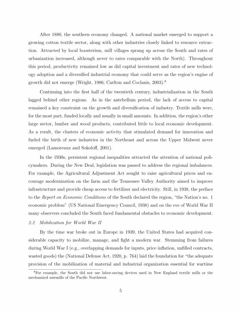
After 1880, the southern economy changed. A national market emerged to support a

growing cotton textile sector, along with other industries closely linked to resource extrac-

tion. Attracted by local boosterism, mill villages sprang up across the South and rates of

urbanization increased, although never to rates comparable with the North). Throughout

this period, productivity remained low as did capital investment and rates of new technol-

ogy adoption and a diversified industrial economy that could serve as the region’s engine of

growth did not emerge (Wright, 1986; Carlton and Coclanis, 2003).8

Continuing into the first half of the twentieth century, industrialization in the South

lagged behind other regions. As in the antebellum period, the lack of access to capital

remained a key constraint on the growth and diversification of industry. Textile mills were,

for the most part, funded locally and usually in small amounts. In addition, the region’s other

large sector, lumber and wood products, contributed little to local economic development.

As a result, the clusters of economic activity that stimulated demand for innovation and

fueled the birth of new industries in the Northeast and across the Upper Midwest never

emerged (Lamoreaux and Sokoloff, 2001).

In the 1930s, persistent regional inequalities attracted the attention of national poli-

cymakers. During the New Deal, legislation was passed to address the regional imbalances.

For example, the Agricultural Adjustment Act sought to raise agricultural prices and en-

courage modernization on the farm and the Tennessee Valley Authority aimed to improve

infrastructure and provide cheap access to fertilizer and electricity. Still, in 1938, the preface

to the Report on Economic Conditions of the South declared the region, “the Nation’s no. 1

economic problem” (US National Emergency Council, 1938) and on the eve of World War II

many observers concluded the South faced fundamental obstacles to economic development.

2.2 Mobilization for World War II

By the time war broke out in Europe in 1939, the United States had acquired con-

siderable capacity to mobilize, manage, and fight a modern war. Stemming from failures

during World War I (e.g., overlapping demands for inputs, price inflation, unfilled contracts,

wasted goods) the (National Defense Act, 1920, p. 764) laid the foundation for “the adequate

provision of the mobilization of material and industrial organization essential for wartime

8For example, the South did not use labor-saving devices used in New England textile mills or themechanized sawmills of the Pacific Northwest.

5

need”. The results were impressive. Between 1939 and 1945, American manufacturers pro-

duced over 300,000 aircraft, 6,000 military ships and merchant vessels, nearly 90,000 tanks

and 350,000 trucks, as well as 6.5 million rifles and 40 billion bullets, to equip 16 million

servicemen (Klein, 2013, pp. 515-516).

At first, mobilization proceeded slowly. For example, in 1939 and 1940, toolmakers were

putting out fewer than 25,000 pieces of equipment per year and the rate of production actually

decreased near the end of 1941 (Klein, 2013, pp. 65-66, 265).9 With the attack on Pearl

Harbor the pace of mobilization accelerated and by the end of 1942 the majority of new war

plants were built or construction was underway. Roughly half of the facilities producing war-

related goods were located in the industrialized Northeast and Upper Midwest. However, for

a variety of reasons, including patronage, security, congestion, weather, and the availability

of labor, raw materials and land, other regions (e.g., the South and West) also received a

substantial portion of spending on contracts and capital (Koistinen, 2004, p. 298).

By the end of the war spending on supply contracts and investment in new facilities

and equipment in the South was more than $20 billion. Although the South as a whole

received less than other regions and southern cities received a smaller share than Detroit,

Buffalo, Chicago, and Los Angeles, the relative gains were substantial.10 The southern trade

magazine, Manufactures’ Record, routinely boasted, “South’s expansion breaks all records”

(quoted in Schulman, 1991, p. 95). Capital expenditures in the South, which made up

roughly one-tenth of the national total in the prewar period, nearly doubled during the war.

In total, the South accounted for 23.1 percent of wartime plant construction and 17.6 of

expansions (US War Production Board, 1945; Deming and Stein, 1949).

In some industries the South enjoyed a particular boom. The region dominated syn-

thetic rubber and developed new competencies in steel and non-ferrous metals. Combat in

the Pacific had cut off most supplies of natural rubber; alcohol and petroleum were neces-

sary inputs into synthetic rubber and both were available in the South. And although the

9To put the extent of the war-created demand in context, “two of three war factories built by thegovernment and operated by Studebaker, for example, each required 3,488 pieces of equipment; the thirdneeded 13,000 machines”.

10Figure A1 plots the share of value-added by manufacturing in 1940 against the share of wartime capitalexpenditures for counties in the South and elsewhere. On average, the figure shows that the South receiveda share of investment spending greater than what would be predicted by its prewar share of manufacturingactivity.

6

Figure 2: Trends in Aggregate Manufacturing in the US South

010

020

030

040

0Es

tabl

ishm

ents

(191

9=10

0)

1920 1930 1940 1950 1960Year

A. Establishments

010

020

030

040

0Em

ploy

men

t (19

19=1

00)

1920 1930 1940 1950 1960Year

B. Employment

010

020

030

040

0W

age

Bill

(191

9=10

0)

1920 1930 1940 1950 1960Year

C. Wage Bill

010

020

030

040

0Va

lue-

Add

ed (1

919=

100)

1920 1930 1940 1950 1960Year

D. Value-Added

Notes: Each panel shows the given variable relative to its value in 1919. The values in Panel Cand Panel D are in 2014 dollars.Source: Data are from Haines (2010).

iron and steel industry continued to concentrate in the cities of the Upper Midwest, new

centers were established along the Gulf Coast. The war created at least temporary clus-

ters in other industries as well (e.g., aircraft in Marietta, Georgia, shipbuilding in Panama

City, Florida). In general, the wartime expansion accounted for a large portion of the newly

available manufacturing capacity (Schulman, 1991; Combes, 2001; Colten, 2001).

The pace of industrial expansion during wartime led one observer to declare that by

the end of the war, “The South, therefore, in January 1945 was no longer the nation’s No.

1 economic problem” (Rauber, 1946, p. 1). Indeed, the changes in southern manufacturing

shown in Figure 2 indicate clear differences in terms of manufacturing establishments, em-

ployment, wage bill, and value-added. Still, the specific link between mobilization for World

War II, increased economic activity during the war, and the growth of manufacturing in the

South in the postwar period is an open question.

7

3 Theoretical Model

This section uses a simple theoretical model to illustrate the relationship between mo-

bilization for World War II and postwar manufacturing.11 The model has one manufacturing

sector and firms in county c choose labor Nc, capital Kc, and land Xc, to solve the following

problem:

maxNc,Kc,Xc

f(ωc, Nc, Kc, Xc)− pNc Nc − pKc Kc − pXc Xc

where pNc , pKc , and pXc denote the price of labor, capital, and land, respectively. The ωc term

is a productivity shifter that is county-specific and, in part, depends on the number of new

facilities constructed during mobilization for World War II. Manufacturing firms sell their

output in international markets, which is normalized to one, and purchase capital services

in international markets so pKc is exogenous to local demand. The supply of land is fixed in

each county c.12 The supply of labor to firms in c is determined by the number of workers

residing in the county and the workers’ indirect utility is a function of wages, the cost of

housing, and the value of local amenities. Workers are freely mobile across counties.

During World War II, manufacturing productivity increased due to wartime investment

embodying new technology and forms of industrial organization. After the war, capital-

owned by the government was sold off to private firms, usually at a discount, and firms

that received capital subsidies as a result of production for government contracts redirected

inputs toward output for consumer markets. In the absence of consumption disamenities

or agglomeration spillovers, the increase in productivity due to mobilization for World War

II increases [CHECK tense] labor demand and, correspondingly, wages and housing costs.

However, the war may have led to a deterioration in the quality of housing, hospitals, schools,

etc., and therefore offset the gains in productivity. Alternatively, the war may have generated

economies of agglomeration through improvements in worker training, intermediate input

markets, transportation, and technology, that continued to benefit manufacturers in the

postwar period. As a result, wages may increase further (i) to compensate for a decline in

the value of consumption amenities or (ii) despite rising local input prices in response to the

11The model here follows the exposition in Hornbeck and Keskin (forthcoming).12This assumption is not too restrictive if access to capital markets is similar across all counties or if

differences are constant within a county over time.

8

lasting benefits from the war economy.

To summarize the impact of mobilization for World War II, consider the change in

manufacturing profits in the short run by taking the total derivative of profits with respect

to war-related facilities construction assuming that firms are price taker and pay all inputs

according to their marginal product:

dΠc

dWc

=

(∂f

∂ωc

× ∂ωc

∂Wc

)− ∂pNc∂Wc

N∗ − ∂pXc∂Wc

X∗ (1)

The first term on the right-hand side of equation (1) captures the net of the positive effects

that work through improvements in worker training, intermediate input markets, transporta-

tion, and technology, and the negative effects that result from the deterioration of the quality

of housing, hospitals, schools, etc. The last two terms capture the effect of changes in local

input prices. The empirical analysis tests the predictions implied by equation (1) using data

on aggregate manufacturing, the number of establishments and employment by sector, and

the cost of housing.

4 Data

The data for the empirical analysis are drawn from several sources. First, county-

level information on aggregate manufacturing, wholesale and retail trade, and the housing

sector is taken from (Haines, 2010). In particular, I make use of information on value-added,

employment, and the number of establishments for manufacturing in 1919, 1929, 1939, 1947,

1954, and 1958. Similarly, for the wholesale and retail sectors I use information on total

sales, employment, and establishment over the same period. Second, I digitized county-level

information on the number of establishments by manufacturing sector from various years of

the Census of Manufactures as well as the Industrial Market Data Handbook of the United

States.

Third, data on the construction and location of investment in structures were collected

from War Manufacturing Facilities Authorized through December 1944 by State and County

published by the War Production Board.13 These data provide the most comprehensive view

of individual investment projects during mobilization for World War II. In particular, the

13I identify investment in structures by summing the number projects listed in War Manufacturing Facil-ities, which excludes projects valued at less than $25,000.

9

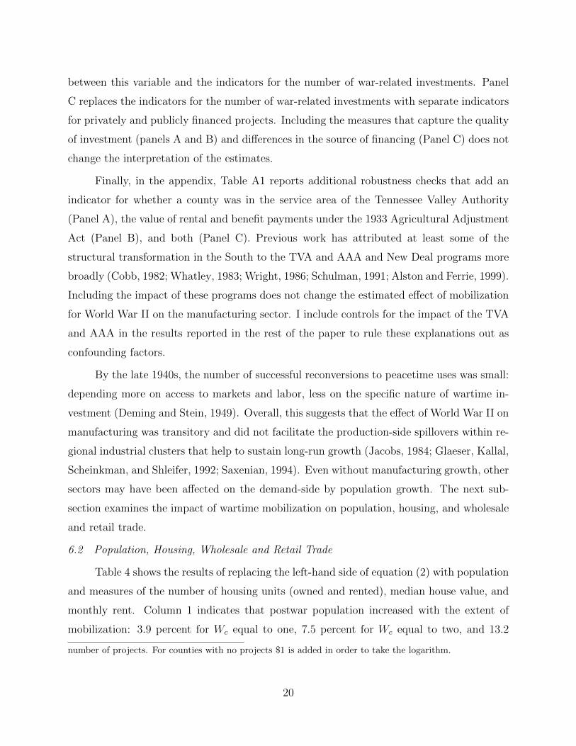
Figure 3: Location of WWII Facilities in the US South

Notes: The dots (in blue) show the location of investment in structures during World War II.Source: See text of Section 4.

fact that the data end in December 1944 is not too concerning since most new construction

was already planned or underway by this time and these are included in War Manufacturing

Facilities. These data also indicate whether the source of financing was directly public or

private and give the month and year the new capital investment became available. Although

some new establishments were financed directly by the private sector, the owner still benefited

from indirect subsidies due to, for example, accelerated depreciation. For this reason, in the

main results I use both types of investment and later in the paper as robustness show the

results for public and private separately. I also show results by the average cost per project

to give a sense of how heterogeneity in the quality or size of investment during wartime may

have affected the value of investment in the postwar period.

Finally, to construct a measure of prewar manufacturing capacity related to military

production I use the Industrial Mobilization Plan collected by Fishback and Cullen (2013).

These data give the number of establishment assigned to each branch of the military in

the event of war mobilization plans set up in the 1930s from the US Joint Army and Navy

Munitions Board (1938). As additional county-level controls, I include information from

10

1940 on population density, the share of population living urban area as well as the foreign

and African-American population shares from Haines (2010).

The empirical analysis uses all counties in the southern states, which include Alabama,

Arkansas, Delaware, Florida, Georgia, Kentucky, and Louisiana, Maryland, Mississippi,

North Carolina, Oklahoma, South Carolina, Tennessee, Texas, Virginia, and West Virginia.

The result is a balanced panel of 1,272 counties. Figure 3 shows the city of each establish-

ment constructed as part of mobilization for World War II overlayed on the 1920 county

boundaries. The total number investment projects in the South during World War II was

1,658. The map in Figure 3 indicates at least one facility was located in each southern state:

Texas had the most at 437 and Delaware had the fewest at 35. For the empirical analysis I

construct a county-level variable, Wc, by aggregating these city-level observations.

5 Empirical Framework and Prewar Trends

The empirical analysis quantifies the relative magnitude of spillovers from investment

in structures due to mobilization for World War II. Specifically, I regress a manufacturing

outcome, Yct, for county c and year t on the indicators for the number of newly constructed

manufacturing facilities during World War II:

Yc,t = αc + αst + β1t1{Wc = 1}+ β2t1{Wc = 2}+ β3t1{Wc ≥ 3}+ ΓtXc + εc,t (2)

The excluded variable is an indicator for Wc equal to zero, so that the estimated βs capture

the difference relative to counties that had no war-related construction. In addition, these

indicators are interacted with year effects for each postwar year in the sample (i.e., 1947,

1954, and 1958) to trace out changes over time in the impact of mobilization for World War

II.

Equation (2) includes additional controls for prewar differences in county character-

istics that may predict differential growth in the postwar period. The vector Xc includes

indicators for the number of facilities allocated under the Industrial Mobilization Plan as well

as the population density and the African-American, foreign, and urban shares of the county

population in 1940. These characteristics are interacted with year fixed effects to allow for

differences in the rate of conditional convergence. Differencing equation (2) controls time-

invariant differences in county characteristics. State-year fixed effects control unobserved

11

differences at the state level that impact regional industrialization. For the postwar period,

changes in state policy following the passage for Taft-Hartley in 1947 played a substantial

role in the growth of manufacturing shown in Figure 2 (see Cobb, 1982; Holmes, 1998).

Table 1 presents summary statistics for the aggregate manufacturing outcomes used in

this study. Each column of Panel A shows the results from regressing the given manufacturing

outcome (in log) measured in 1939 on indicator for the number of World War II investments,

Wc ∈ (1, 2, 3+). The results reveal substantial differences between counties in terms of

prewar manufacturing and the extent of mobilization for World War II. County fixed effects,

state-year fixed effects, and controls for 1940 county characteristics included in equation

(2) adjust for these differences. Importantly, in Panel B of Table 1, comparing the prewar

trends across counties with Wc ∈ (1, 2, 3+) relative to Wc equal to zero reveal no statistically

significant differences for any outcome or level of mobilization. These results support the

validity of the postwar comparisons that are the focus of this paper.

To be clear, the identifying assumption for the βs in equation (2) is that in the absence

of new facility construction during World War II, relative changes in the southern economy

would have followed their prewar trajectory. In practice, this assumption is violated if war

planners decided the placement of new facilities with domestic goals in mind. The discussion

of the mobilization program by Koistinen (2004), in particular, the centralized control in the

military rather than the civilian bureaucracy, suggests the location of new facilities was not

motivated by economic development objectives. Instead, planners aimed to maximize the

production of standardized and relatively high quality products. In this case, the key con-

cern is that characteristics correlated with planners’ ability to achieve these objectives were

also correlated with growth potential. Controls for the Industrial Mobilization Plan ensure

that my estimates capture the effect new facilities construction due to actual mobilization,

not industrial potential based on prewar capacity; controls for latitude, longitude, and soil

quality capture changes in southern agriculture that may have influenced industrial develop-

ment. Finally, as robustness, I also discuss separate estimates that control for aspects of the

New Deal that may have influenced the growth of manufacturing either directly through new

infrastructure (e.g., the Tennessee Valley Authority) or policies intended to modernize agri-

culture (e.g., the Agricultural Adjustment Act). Structural transformation in the 1930s and

the contribution of the New Deal have been studied extensively (e.g., Whatley, 1983; Caselli

12

Table 1: Prewar Differences by Number of World War II Facilities

Emp. Wage Bill Value-Added

(1) (2) (3)

Panel A: Diff.

Relative to Wc = 0

1{Wc = 1} 0.443 0.464 0.473

(0.187) (0.253) (0.252)

1{Wc = 2} 0.687 0.735 0.711

(0.176) (0.288) (0.281)

1{Wc ≥ 3} 0.989 1.217 1.204

(0.204) (0.182) (0.161)

Panel B: Trend

Relative to Wc = 0

1{Wc = 1} × t 0.002 -0.007 -0.007

(0.008) (0.015) (0.016)

1{Wc = 2} × t -0.001 -0.009 -0.009

(0.011) (0.022) (0.021)

1{Wc ≥ 3} × t 0.002 -0.007 -0.008

(0.010) (0.025) (0.029)

Notes: The table presents differences across counties in terms of prewar aggregate manufacturing charac-teristics. Panel A shows the difference in 1939 between counties with one, two, or more than three WorldWar II investment projects, i.e., Wc ∈ (1, 2, 3+) relative to counties with zero, i.e., Wc = 0. The estimatesin each column come from the same regression, which includes state fixed effects and county characteristics.Panel B shows the difference in prewar trend between counties with Wc ∈ (1, 2, 3+) relative to counties withWc = 0. The years included are 1919, 1929, and 1939. The estimates in each column come from the sameregression, which includes state-year and county fixed effects as well as county characteristics. Standarderrors (in parentheses) are clustered at the state level and regressions are weighted by county population ineach year. The number of sample counties is 1,272.Source: For a description of the data and variables included as county characteristics see text of Section 4.

and Coleman, 2001; Fishback, Horrace, and Kantor, 2005; Hornbeck and Naidu, 2014). For

the purposes of this study, it is important not to attribute the effects of changes underway

by the early 1940s to the effect of World War II.14

6 Results

6.1 Manufacturing

The panels of Table 2 show the results of estimating different versions of equation

(2) for several aggregate manufacturing outcomes. The estimates reported are relative to

14Indeed, in revising the early literature for the impact of World War II on industrial development instates along the Pacific Coast, Rhode (2000, 2003) emphasizes the small role of the war compared to forcesalready at work in the 1920s.

13

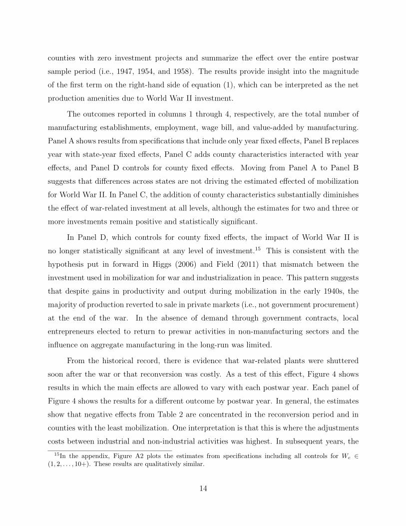
counties with zero investment projects and summarize the effect over the entire postwar

sample period (i.e., 1947, 1954, and 1958). The results provide insight into the magnitude

of the first term on the right-hand side of equation (1), which can be interpreted as the net

production amenities due to World War II investment.

The outcomes reported in columns 1 through 4, respectively, are the total number of

manufacturing establishments, employment, wage bill, and value-added by manufacturing.

Panel A shows results from specifications that include only year fixed effects, Panel B replaces

year with state-year fixed effects, Panel C adds county characteristics interacted with year

effects, and Panel D controls for county fixed effects. Moving from Panel A to Panel B

suggests that differences across states are not driving the estimated effected of mobilization

for World War II. In Panel C, the addition of county characteristics substantially diminishes

the effect of war-related investment at all levels, although the estimates for two and three or

more investments remain positive and statistically significant.

In Panel D, which controls for county fixed effects, the impact of World War II is

no longer statistically significant at any level of investment.15 This is consistent with the

hypothesis put in forward in Higgs (2006) and Field (2011) that mismatch between the

investment used in mobilization for war and industrialization in peace. This pattern suggests

that despite gains in productivity and output during mobilization in the early 1940s, the

majority of production reverted to sale in private markets (i.e., not government procurement)

at the end of the war. In the absence of demand through government contracts, local

entrepreneurs elected to return to prewar activities in non-manufacturing sectors and the

influence on aggregate manufacturing in the long-run was limited.

From the historical record, there is evidence that war-related plants were shuttered

soon after the war or that reconversion was costly. As a test of this effect, Figure 4 shows

results in which the main effects are allowed to vary with each postwar year. Each panel of

Figure 4 shows the results for a different outcome by postwar year. In general, the estimates

show that negative effects from Table 2 are concentrated in the reconversion period and in

counties with the least mobilization. One interpretation is that this is where the adjustments

costs between industrial and non-industrial activities was highest. In subsequent years, the

15In the appendix, Figure A2 plots the estimates from specifications including all controls for Wc ∈(1, 2, . . . , 10+). These results are qualitatively similar.

14

Table 2: Impact of World War II on Manufacturing


(1) (2) (3)

Panel A:

Controls: αt

1{Wc = 1} × postt 0.300 0.195 0.232

(0.293) (0.306) (0.314)

1{Wc = 2} × postt 1.022 1.117 1.176

(0.326) (0.368) (0.374)

1{Wc ≥ 3} × postt 2.874 3.283 3.460

(0.357) (0.401) (0.411)

Panel B:

Controls: αst

1{Wc = 1} × postt 0.417 0.308 0.358

(0.257) (0.285) (0.288)

1{Wc = 2} × postt 1.107 1.218 1.314

(0.301) (0.339) (0.335)

1{Wc ≥ 3} × postt 3.002 3.378 3.545

(0.412) (0.441) (0.434)

Panel C:

Controls: αst, Xc

1{Wc = 1} × postt 0.112 -0.038 0.003

(0.147) (0.180) (0.180)

1{Wc = 2} × postt 0.574 0.615 0.677

(0.101) (0.134) (0.140)

1{Wc ≥ 3} × postt 0.821 0.909 0.974

(0.200) (0.165) (0.162)

Panel D:

Controls: αc, αst, Xc

1{Wc = 1} × postt -0.048 -0.084 -0.077

(0.038) (0.070) (0.068)

1{Wc = 2} × postt 0.004 -0.017 0.028

(0.049) (0.091) (0.088)

1{Wc ≥ 3} × postt -0.024 -0.120 -0.089

(0.033) (0.085) (0.082)

Notes: Each panel gives the results of estimating a version equation (2). The columns contain the resultsfor different manufacturing outcomes: employment (column 1), wage bill (column 2), and value-added bymanufacturing (column 3). Panel A includes only year fixed effects, Panel B includes state-year fixed effects,Panel C adds county characteristics interacted with year fixed effects, and Panel D is the first differenceof equation (2) to control for time-invariant county characteristics. Standard errors (in parentheses) areclustered at the state level and regressions are weighted by county population in each year. The yearsincluded are 1919, 1929, 1939, 1947, 1954, and 1958. The number of sample counties is 1,272.Source: For a description of the data and variables included as county characteristics see text of Section 4.

15

Figure 4: Impact of World War II on Manufacturing by Year-.8

-.40

.4

1 2 3number of war plants

1947

-.8-.4

0.4


1954

-.8-.4

0.4


1958

A. Employment

-.8-.4

0.4


1947

-.8-.4

0.4


1954

-.8-.4

0.4


1958

B. Wage Bill

-.8-.4

0.4


1947

-.8-.4

0.4


1954

-.8-.4

0.4


1958

C. Value-Added

Notes: Each panel shows the estimated coefficient for each variable along the 90 percent confidence intervalbased on standard errors clustered at the state level. All regressions are weighted by county population ineach year. The years included are 1919, 1929, 1939, 1947, 1954, and 1958. The number of sample countiesis 1,272.Source: For a description of the data and variables included as county characteristics see text of Section 4.

effect tends to be close to zero and statistically insignificant. The limited effect of war-

related investment suggest that it was too specific to military production needs or utilized

to the point of near complete depreciation as a result of two- or three-shift runs during the

mobilization period (Higgs, 2006; Field, 2011; Rockoff, 2012). This is consistent with the

substantial discounts tabulated by White (1980) that were applied to the sale of surplus

property in the postwar period.16

In Figure 5, Panel A presents the results for each postwar year for the number of man-

ufacturing establishments. The number of establishments was more in 1958 relative to the

prewar period. To assess the impact of wartime investment across different manufacturing

sectors, the remaining panels of Figure 5 disaggregates the results for the number of establish-

ments by fourteen sectors. This is useful because even in the absence of substantial changes

in the aggregate number of establishments, the war may have facilitated the reallocation of

activity across sectors. In the context of the mid-twentieth century South, this effect may

be particularly important since a key focus of contemporary policy makers and scholars was

the concentration of the region’s industrial activity in low wage, low value-added sectors.

Overall, there is little evidence that reallocation is underlying the changes in southern man-

ufacturing in the postwar period. Following the end of the war the number of establishments

in rubber goods, metals, machine tools, and transportation equipment was higher. However,

16This is line with evidence presented by Kline and Moretti (2014b) for the Tennessee Valley Authority,which suggests that the program’s benefits were due to the direct investment in infrastructure and notthrough the accumulation of agglomeration economies.

16

Figure 5: Impact of World War II on Manufacturing Establishments by Sector and Year

-.8-.4

0.4


1947

-.8-.4

0.4


1954

-.8-.4

0.4


1958

A. Total Establishments

-2-1

.6-1

.2-.8

-.40

.4.8

1.2

1.6

2


1947

-2-1

.6-1

.2-.8

-.40

.4.8

1.2

1.6

2


1954

-2-1

.6-1

.2-.8

-.40

.4.8

1.2

1.6

2


1958

B. Food

-2-1

.6-1

.2-.8

-.40

.4.8

1.2

1.6

2


1947

-2-1

.6-1

.2-.8

-.40

.4.8

1.2

1.6

2


1954

-2-1

.6-1

.2-.8

-.40

.4.8

1.2

1.6

2


1958

C. Textiles

-2-1

.6-1

.2-.8

-.40

.4.8

1.2

1.6

2


1947

-2-1

.6-1

.2-.8

-.40

.4.8

1.2

1.6

2


1954

-2-1

.6-1

.2-.8

-.40

.4.8

1.2

1.6

2


1958

D. Lumber

-2-1

.6-1

.2-.8

-.40

.4.8

1.2

1.6

2


1947

-2-1

.6-1

.2-.8

-.40

.4.8

1.2

1.6

21 2 3

number of war plants

1954

-2-1

.6-1

.2-.8

-.40

.4.8

1.2

1.6

2


1958

E. Paper

-2-1

.6-1

.2-.8

-.40

.4.8

1.2

1.6

2


1947

-2-1

.6-1

.2-.8

-.40

.4.8

1.2

1.6

2


1954

-2-1

.6-1

.2-.8

-.40

.4.8

1.2

1.6

2


1958

F. Printing

-2-1

.6-1

.2-.8

-.40

.4.8

1.2

1.6

2


1947

-2-1

.6-1

.2-.8

-.40

.4.8

1.2

1.6

2


1954

-2-1

.6-1

.2-.8

-.40

.4.8

1.2

1.6

2


1958

G. Chemicals

-2-1

.6-1

.2-.8

-.40

.4.8

1.2

1.6

2


1947

-2-1

.6-1

.2-.8

-.40

.4.8

1.2

1.6

2


1954-2

-1.6

-1.2

-.8-.4

0.4

.81.

21.

62


1958

H. Petroleum

-2-1

.6-1

.2-.8

-.40

.4.8

1.2

1.6

2


1947

-2-1

.6-1

.2-.8

-.40

.4.8

1.2

1.6

2


1954

-2-1

.6-1

.2-.8

-.40

.4.8

1.2

1.6

2


1958

I. Rubber

-2-1

.6-1

.2-.8

-.40

.4.8

1.2

1.6

2


1947

-2-1

.6-1

.2-.8

-.40

.4.8

1.2

1.6

2


1954

-2-1

.6-1

.2-.8

-.40

.4.8

1.2

1.6

2


1958

J. Leather

-2-1

.6-1

.2-.8

-.40

.4.8

1.2

1.6

2


1947

-2-1

.6-1

.2-.8

-.40

.4.8

1.2

1.6

2


1954

-2-1

.6-1

.2-.8

-.40

.4.8

1.2

1.6

2


1958

K. Stone

-2-1

.6-1

.2-.8

-.40

.4.8

1.2

1.6

2


1947

-2-1

.6-1

.2-.8

-.40

.4.8

1.2

1.6

2


1954

-2-1

.6-1

.2-.8

-.40

.4.8

1.2

1.6

2


1958

L. Metals

-2-1

.6-1

.2-.8

-.40

.4.8

1.2

1.6

2


1947

-2-1

.6-1

.2-.8

-.40

.4.8

1.2

1.6

2


1954

-2-1

.6-1

.2-.8

-.40

.4.8

1.2

1.6

2


1958

M. Machinery

-2-1

.6-1

.2-.8

-.40

.4.8

1.2

1.6

2


1947

-2-1

.6-1

.2-.8

-.40

.4.8

1.2

1.6

2


1954

-2-1

.6-1

.2-.8

-.40

.4.8

1.2

1.6

2


1958

N. Trans. Eq.

-2-1

.6-1

.2-.8

-.40

.4.8

1.2

1.6

2


1947

-2-1

.6-1

.2-.8

-.40

.4.8

1.2

1.6

2


1954

-2-1

.6-1

.2-.8

-.40

.4.8

1.2

1.6

2


1958

O. Misc.

Notes: Each panel shows the estimated coefficient for each variable along the 90 percent confidence intervalbased on standard errors clustered at the state level. All regressions are weighted by county population ineach year. The years included in Panel A are 1919, 1929, 1939, 1947, 1954, and 1958; for the remainingpanels (by sector) the years are 1935, 1939, 1947, 1954, and 1958. The number of sample counties is 1,272.Source: For a description of the data and variables included as county characteristics see text of Section 4.

17

ultimately, the results in Figure 5 suggest that reallocation of manufacturing activity across

sectors due to World War II was short-lived and, in any case, not widespread.

Focusing on a particular example, Combes (2001, pp. 28-33) describes the efforts on

the part of local politicians that led to the opening of a Bell Aircraft in Marietta, Georgia, in

early 1942. The plant, which manufactured B-29s during the war, grew from 1,179 employees

in the beginning to 17,094 by the end of 1943 and eventually reached an employment peak

above 20,000. In part, the tremendous growth of manufacturing reflected in this and other

accounts of the wartime South (see Schulman, 1991) helped reinforce the view of structural

transformation fueled by World War II investment. In the case of Bell Aircraft in Georgia

and other newcomers to advanced manufacturing across the South, the war appeared to

bring demand and training for new skills. Nevertheless, despite attempts to find a postwar

use for the plant, $60 million in payroll disappeared and the $47 million investment was

converted for storage for military surplus in the immediate aftermath of the war.

The plant in Marietta eventually housed operations for the production of the Lockheed

C-130, C-141, and C-5, although “in contrast to a successful private sector manufacturer,

the Marietta plant looks more like a mission-oriented federal laboratory. . . ” (Combes, 2001,

p. 39). More generally, the lesson that the potential uses for Marietta plant were limited

seemed to also apply to other wartime investment across the South.

So far, the results treat investment projects as homogeneous. However, there may

have been substantial differences in the quality and type of investment across countries. In

particular, my data include information on (i) the cost of projects and (ii) whether the direct

course of financing was private or public. Differences in (i) are informative about utilization

and quality, while differences in (ii) indicate the ability of firms to make investments that

were more (private) or less (public) likely to be compatible with peacetime production.17

To examine the impact of investment type and quality, I estimate specifications similar

to equation (2) and report the results in Table 3. Panel A includes a control variable for

the average cost per investment project in a given county.18 Panel B includes interactions

17Deming and Stein (1949, p. 3, 12) describe how both privately and publicly financed project ultimatelyreceived some form of government subsidy indirectly through the accelerated depreciation provisions of the1940 Second Revenue Act or directly. In addition, privately financed projects were subject to less oversightand more likely to be built with dual purposes to meet wartime demand and be useful in peacetime.

18This variable was constructed by summing the total cost of all projects in county c and dividing by the

18

Table 3: Impact of World War II on Manufacturing by Quality and Type


(1) (2) (3)

Panel A:

1{Wc = 1} × postt -0.027 -0.057 -0.064

(0.137) (0.160) (0.172)

1{Wc = 2} × postt 0.026 0.013 0.042

(0.152) (0.170) (0.181)

1{Wc ≥ 3} × postt -0.001 -0.089 -0.075

(0.151) (0.150) (0.165)

ln(average cost)c × postt -0.002 -0.003 -0.001

(0.012) (0.013) (0.014)

Panel B:

1{Wc = 1} × postt 0.067 -0.281 -0.374

(0.210) (0.438) (0.452)

1{Wc = 2} × postt 0.230 0.276 0.285

(0.185) (0.260) (0.272)

1{Wc ≥ 3} × postt -0.216 -0.128 -0.040

(0.157) (0.251) (0.297)

ln(average cost)c × 1{Wc = 1} × postt -0.011 0.019 0.028

(0.018) (0.040) (0.042)

ln(average cost)c × 1{Wc = 2} × postt -0.019 -0.025 -0.022

(0.014) (0.019) (0.020)

ln(average cost)c × 1{Wc ≥ 3} × postt 0.016 0.001 -0.004

(0.012) (0.023) (0.027)

Panel C:

1{Publicc = 1} × postt 0.005 0.007 0.000

(0.029) (0.122) (0.119)

1{Publicc = 2} × postt -0.045 -0.075 -0.014

(0.050) (0.066) (0.059)

1{Publicc ≥ 3} × postt 0.106 0.152 0.122

(0.080) (0.063) (0.066)

1{Privatec = 1} × postt -0.049 -0.098 -0.090

(0.039) (0.078) (0.076)

1{Privatec = 2} × postt -0.002 -0.024 0.004

(0.051) (0.100) (0.104)

1{Privatec ≥ 3} × postt -0.018 -0.115 -0.090

(0.032) (0.088) (0.085)

Notes: Each panel adds variables to the specification reported in Panel D of Table 2. Panel A adds the (log)average cost per project in county c, Panel B adds an interaction between (log) average cost per project incounty c and the indicators for the levels of Wc, and Panel C replaces the indicators for Wc with separateindicators for the number of publicly- and privately-financed projects. Standard errors (in parentheses)are clustered at the state level and regressions are weighted by county population in each year. The yearsincluded are 1919, 1929, 1939, 1947, 1954, and 1958 The number of sample counties is 1,272.Source: For a description of the data and variables included as county characteristics see text of Section 4.

19

between this variable and the indicators for the number of war-related investments. Panel

C replaces the indicators for the number of war-related investments with separate indicators

for privately and publicly financed projects. Including the measures that capture the quality

of investment (panels A and B) and differences in the source of financing (Panel C) does not

change the interpretation of the estimates.

Finally, in the appendix, Table A1 reports additional robustness checks that add an

indicator for whether a county was in the service area of the Tennessee Valley Authority

(Panel A), the value of rental and benefit payments under the 1933 Agricultural Adjustment

Act (Panel B), and both (Panel C). Previous work has attributed at least some of the

structural transformation in the South to the TVA and AAA and New Deal programs more

broadly (Cobb, 1982; Whatley, 1983; Wright, 1986; Schulman, 1991; Alston and Ferrie, 1999).

Including the impact of these programs does not change the estimated effect of mobilization

for World War II on the manufacturing sector. I include controls for the impact of the TVA

and AAA in the results reported in the rest of the paper to rule these explanations out as

confounding factors.

By the late 1940s, the number of successful reconversions to peacetime uses was small:

depending more on access to markets and labor, less on the specific nature of wartime in-

vestment (Deming and Stein, 1949). Overall, this suggests that the effect of World War II on

manufacturing was transitory and did not facilitate the production-side spillovers within re-

gional industrial clusters that help to sustain long-run growth (Jacobs, 1984; Glaeser, Kallal,

Scheinkman, and Shleifer, 1992; Saxenian, 1994). Even without manufacturing growth, other

sectors may have been affected on the demand-side by population growth. The next sub-

section examines the impact of wartime mobilization on population, housing, and wholesale

and retail trade.

6.2 Population, Housing, Wholesale and Retail Trade

Table 4 shows the results of replacing the left-hand side of equation (2) with population

and measures of the number of housing units (owned and rented), median house value, and

monthly rent. Column 1 indicates that postwar population increased with the extent of

mobilization: 3.9 percent for Wc equal to one, 7.5 percent for Wc equal to two, and 13.2

number of projects. For counties with no projects $1 is added in order to take the logarithm.

20

Table 4: Impact of World War II on Population and Housing

Owned: Rented:

# Median # Monthly

Population units Value units Rent

(1) (2) (3) (4) (5)

1{Wc = 1} × postt 0.039 -0.005 -0.075 0.001 0.064

(0.028) (0.036) (0.024) (0.029) (0.021)

1{Wc = 2} × postt 0.078 -0.044 -0.075 -0.005 0.025

(0.024) (0.024) (0.025) (0.025) (0.022)

1{Wc ≥ 3} × postt 0.131 -0.015 -0.050 -0.001 0.001

(0.020) (0.030) (0.042) (0.024) (0.024)

Notes: Standard errors (in parentheses) are clustered at the state level and regressions in columns 2 through5 are weighted by county population in each year. The years included are 1929, 1939, 1949, and 1959. Thenumber of sample counties is 1,272.Source: For a description of the data and variables included as county characteristics see text of Section 4.

percent for three or more new facilities. The results in columns 2 through 4 indicate little

change in the number of available non-farm units. Columns 3 and 5 point toward a decrease

in the value of owner-occupied units–consistent with crowding into these areas during the

war accelerating depreciation of the value of the housing stock–and an increase in monthly

rent.

Table 5 shows the results for wholesale and retail trade. From columns 1 through 3,

the war’s effect on wholesale is limited and, in any case, imprecisely estimated. The effect on

the retail sector is consistently positive and, for employment and sales, statistically signifi-

cant for counties with two or more facilities. Together with the increase in population the

results for the retail sector suggest that wartime investment did stimulate growth in local

economies. This is supported by the example from Combes (2001) for Marietta, Georgia.

One interpretation is that investment may have helped to coordinate the placement of gov-

ernment contracts and investment in the postwar period. For example, the research facility

in Marietta, and other installations related to the military, US Atomic Energy Commission,

National Aeronautics and Space Administration, and the Center for Disease Control (US

Public Health Service, various years; Schulman, 1991; Klein, 2013; Downs, 2014). This, in

turn, stimulated local demand.

Note that this mechanism for the impact of World War II is different from the standard

story of southern structural transformation fueled by mobilization. Parts of the mobilization

21

Table 5: Impact of World War II on Wholesale and Retail Trade

Wholesale: Retail:

Estab. Emp. Sales Estab. Emp. Sales

(1) (2) (3) (4) (5) (6)

1{Wc = 1} × postt 0.009 -0.015 -0.146 0.018 0.038 0.048

(0.050) (0.187) (0.139) (0.023) (0.045) (0.039)

1{Wc = 2} × postt 0.052 -0.026 -0.027 0.023 0.049 0.051

(0.047) (0.110) (0.123) (0.018) (0.017) (0.019)

1{Wc ≥ 3} × postt 0.073 -0.136 -0.026 0.050 0.060 0.061

(0.050) (0.179) (0.111) (0.025) (0.021) (0.020)

Notes: Standard errors (in parentheses) are clustered at the state level and regressions are weighted bycounty population in each year. The years included are 1929, 1939, 1948, and 1958 The number of samplecounties is 1,272.Source: See text of Section 4.

program may have facilitated growth in some industries and counties, but this effect was not

consistently positive or statistically significant.

7 Conclusion

Prior to 1940 the development of the American South lagged behind the rest of the

country. Mobilization for World War II stimulated demand for industrial goods and infused

the region with substantial investment in new manufacturing capital. A long-standing ques-

tion in the economic history of the United States is whether war-related investment created

agglomeration economies that stimulated the region’s postwar growth. More generally, the

answer to this question contributes to a large literature on the role of specific government

policies in regional development and economic growth.

In this paper, I combine information on the location of manufacturing facilities con-

structed in the South between 1940 and 1945 with information on aggregate manufacturing

and the number of establishments by sector to examine the impact of the war on southern

industrialization. The results suggest no differential growth in aggregate manufacturing and

limited permanent reallocation of manufacturing activity toward higher value-added sectors

within manufacturing; in rubber goods, metals, machine tools, and transportation equip-

ment there were more establishments immediately following the war, but these effects were

short-lived. This suggests that structural transformation and the growth of manufacturing

in the American South were not the result of mobilization for World War II.

22

The only lasting impact of the war was concentrated in the retail sector and county-

level population, which were up to 6.1 and 13.1 percent larger, respectively. I interpret this

finding as evidence that investment during World War II helped coordinate the placement

of government contracts and investment in the South in the postwar period. The finding

that war-related investment had no effect on the average southern county does not preclude

success stories in more narrowly defined industries or in certain places. Indeed, the histori-

cal record contains evidence for aircraft, aluminum, and synthetic rubber where the role of

the South during and after the war was important; the confidence intervals for the effect

on aggregate manufacturing and by sector suggest substantial variation. I leave these case

studies for future research, and conclude that the evidence does not support a region trans-

formed by mobilization for war. Rather, as on the Pacific Coast, industrialization already

underway continued during the war and the war itself did not lay the foundation for growth

of manufacturing in the American South.

23

References

Daron Acemoglu and Simon Johnson. Unbundling Institutions. Journal of Political Economy,113(5):949–995, 2005.

Lee J. Alston and Joseph P. Ferrie. Southern Paternalism and the American Welfare State:Economics, Politics, and Institutions in the South, 1865-1965. Cambridge UniversityPress, Cambridge, UK, 1999.

Robert J. Barro. Output Effects of Government Purchases. Journal of Political Economy,89(6):1086–1121, 1981.

Robert J. Barro and Xavier Sala-i-Martin. Convergence Across States and Regions. BrookingsPapers on Economic Activity, pages 107–182, 1991.

Robert J. Barro and Xavier Sala-i-Martin. Convergence. Journal of Political Economy, 100(2):223–251, 1992.

Fred Bateman, Jamie Ros, and Jason E. Taylor. Did New Deal and World War II Public Cap-ital Investments Facilitate a ‘Big Push’ in the American South? Journal of Institutionaland Theoretical Economics, 165(2):307–341, 2009.

David L. Carlton and Peter A. Coclanis. The South, The Nation, and The World: Perspec-tives on Southern Economic Development. University of Virginia Press, Charlottesville,VA, 2003.

Francesco Caselli and Wilbur John Coleman. The U.S. Structural Transformation and Re-gional Convergence: A Reinterpretation. Journal of Political Economy, 109(3):584–616,2001.

James C. Cobb. The Selling of the South: The Southern Crusade for Industrial Development,1936-90. Louisiana State University Press, Baton Rouge, LA, 1982.

Craig E. Colten. Texas v. the Petrochemical Industry: Contesting Pollution in an Era of In-dustrial Growth. In Philip Scranton, editor, The Second Wave: Southern Industrializationfrom the 1940s to the 1970s. University of Georgia Press, New York, GA, 2001.

Richard S. Combes. Aircraft Manufacturing in Georgia: A Case Study of Federal IndustrialInvestment. In Philip Scranton, editor, The Second Wave: Southern Industrialization fromthe 1940s to the 1970s. University of Georgia Press, Athens, GA, 2001.

J. Bradford De Long and Lawrence H. Summers. Equipment Investment and EconomicGrowth. Quartlery Journal of Economics, 106(2):445–502, 1991.

Frederick L. Deming and Weldon A. Stein. Disposal Of Southern War Plants. NationalPlanning Association, Washington, DC, 1949.

Matthew L. Downs. Transforming the South: Federal Development in the Tennessee Valley,1915-1960. Louisiana State University Press, Baton Rouge, LA, 2014.

Alexander J. Field. A Great Leap Forward: 1930s Depression and U.S. Economic Growth.Yale University Press, New Haven, CT, 2011.

Price V. Fishback and Joseph A. Cullen. Second World War Spending and Local EconomicActivity in US Counties, 1939-58. Economic History Review, 66(4):975–992, 2013.

Price V. Fishback, William C. Horrace, and Shawn Kantor. Did New Deal Grant ProgramsStimulate Local Economies? A Study of Federal Grants and Retail Sales during the GreatDepression. Journal of Economic History, 65(1):36–71, 2005.

24

Robert W. Fogel and Stanley L. Engerman. Time on the Cross: The Economics of AmericanNegro Slavery. Little, Brown, Boston, MA, 1974.

Andrew D. Foster and Mark R. Rosenzweig. Learning by Doing and Learning from Others:Human Capital and Technical Change in Agriculture. Journal of Political Economy, 103(6):1176–1208, 1995.

Edward L. Glaeser, Hedi D. Kallal, Jose A. Scheinkman, and Andrei Shleifer. Growth inCities. Journal of Political Economy, 100(6):1126–1152, 1992.

Robert J. Gordon. $45 Billion of U.S. Private Investment Has Been Mislaid. AmericanEconomic Review, 59(3):221–238, 1969.

Michael R. Haines. Historical, Demographic, Economic, and Social Data: The united States,1790-2000, volume ICPSR02896-v3. Inter-university Consortium for Political and SocialResearch [distributor], Ann Arbor, MI, 2010.

Robert Higgs. Crisis and Leviathan: Critical Episodes in the Growth of American Govern-ment. Oxford University Press, Oxford, UK, 1989.

Robert Higgs. Private Profit, Public Risk: Institutional Antecedents of the Modern MilitaryProcurement System in the Rearmament Program of 1940-41. In Robert Higgs, editor,Depression, War, and Cold War: Studies in Political Economy. Oxford University Press,Oxford, 2006.

Thomas J. Holmes. The Effect of State Policies on the Location of Manufacturing: Evidencefrom State Borders. Journal of Political Economy, 106(4):667–705, 1998.

Richard Hornbeck and Pinar Keskin. Does Agriculture Generate Local Economic Spillovers?Short-run and Long-run Evidence from Ogallala Aquifer. American Economic Journal:Economic Policy, forthcoming.

Richard Hornbeck and Suresh Naidu. When the Levee Breaks: Black Migration and Eco-nomic Devleopment in the American South. American Economic Review, 104(3):963–990,2014.

Jane Jacobs. Cities and the Wealth of Nations: Principles of Economic Life. Random House,New York, NY, 1984.

Charles I. Jones. Intermediate Goods and Weak Links in the Theory of Economic Develop-ment. American Economic Journal: Macroeconomics, 3(2):1–28, 2011.

Sukkoo Kim. Expansion of Markets and the Geographic Distribution of Economic Activities:The Trends in U.S. Regional Manufacturing Structure, 1860-1987. Quarterly Journal ofEconomics, 110(4):881–908, 1995.

Sukkoo Kim. Economic Integration and Convergence: U.S. Regions, 1840-1987. Journal ofEconomic History, 58(3):659–683, 1998.

Carl Kitchens. The Role of Publicly Provided Electricity in Economic Development: TheExperience of the Tennessee Valley Authority, 19291955. Journal of Economic History, 74(2):389–419, 2014.

Maury Klein. A Call to Arms: Mobilizing America for World War II. Bloomsbury Press,New York, NY, 2013.

Patrick Kline and Enrico Moretti. Local Economic Development, Agglomeration Economiesand the Big Push: 100 Years of Evidence from the Tennessee Valley Authority. Quarterly

25

Journal of Economics, 129(1):275–331, 2014a.

Patrick Kline and Enrico Moretti. Local Economic Development, Agglomeration Economiesand the Big Push: 100 Years of Evidence from the Tennessee Valley Authority. QuarterlyJournal of Economics, 129(1):275–331, 2014b.

Paul A.C. Koistinen. Arsenal of World War II: The Political Economy of American Warfare,1940-1945. University Kansas Press, Lawrence, KS, 2004.

Naomi R. Lamoreaux and Kenneth L. Sokoloff. Market Trade in Patens and the Rise of aClass of Specialized Inventors in the Nineteenth-Century United States. American Eco-nomic Review, 91(3):39–44, 2001.

Ann Markusen, Peter Hall, Scott Campbell, and Sabina Deitrick. The Rise of the Gunbelt:The Military Remapping of Industrial America. Oxford University Press, Oxford, UK,1991.

Kris Mitchener and Ian W. McLean. U.S. Regional Growth and Convergence, 1880-1980.Journal of Economic History, 59(4):1016–1042, 1999.

Kris Mitchener and Ian W. McLean. The Productivity of U.S. States since 1880. Journal ofEconomic Growth, 8(1):73–114, 2003.

Kevin M. Murphy, Andrei Shleifer, and Robert W. Vishny. Industrialization and the BigPush. Journal of Political Economy, 97(5):1003–1026, 1989.

Gerald D. Nash. The American West Transformed: The Impact of the Second World War.Indiana University Press, Bloomington, 1985.

Gerald D. Nash. World War II and the West: Reshaping the Economy. University ofNebraska Press, Lincoln, 1990.

National Defense Act. U. S. Statutes at Large, 41:759–811, 1920.

Douglass C. North. Structure and Change in Economic History. WW Norton, New York,NY, 1981.

Mancur Olson. Power And Prosperity: Outgrowing Communist And Capitalist Dictatorships.Basic Books, New York, NY, 2000.

Valerie A. Ramey and Matthew D. Shapiro. Displaced Capital: A Study of Aerospace PlantClosings. Journal of Political Economy, 109(5):958–992, 2001.

Earle L. Rauber. Economic Appraisal of the Postwar South. Monthly Review of the FederalReserve Bank of Atlanta, 31(1):1–2, 1946.

Paul W. Rhode. California in the Second World War. In Roger Lotchin, editor, The WayWe Really Were: The Golden State in the Second Great War. University of Illinois Press,Urbana, 2000.

Paul W. Rhode. After the War Boom: Reconversion on the Pacific Coast, 1943-1949. InTimothy Guinnane William Sundstrom and Warren Whatley, editors, History Matters:Essays on Economic Growth, Technology, and Demographic Change. Stanford UniversityPress, Stanford, 2003.

Hugh Rockoff. America’s Economic Way of War: War and the US Economy from theSpanish-American War to the Persian Gulf War. Cambridge University Press, Cambridge,UK, 2012.

Paul M. Romer. Increasing Returns and Long-Run Growth. Journal of Political Economy,

26

94(5):1002–1037, 1986.

AnnaLee Saxenian. Regional Advantage: Culture and Competition in Silicon Valley andRoute 128. Harvard University Press, Cambridge, MA, 1994.

Bruce J. Schulman. From Cotton Belt to Sunbelt: Federal Policy, Economic Development,and the Transformation of the South, 1938-1980. Oxford University Press, Oxford, UK,1991.

Chad Turner, Robert Tamura, Sean E. Mulholland, and Scott Baier. Education and Incomeof the States of the United States: 1840-2000. Journal of Economic Growth, 12(2):101–158,2007.

US Joint Army and Navy Munitions Board. Industrial Mobilization Plan: Revision of 1938.Government Printing Office, Washington, DC, 1938.

US National Emergency Council. Report on Economic Conditions of the South. GovernmentPrinting Office, Washington, DC, 1938.

US Public Health Service. Malaria Control in War Areas Report. Office of GovernmentPrinting, Washington DC, various years.

US War Production Board. War Manufacturing Facilities Authorized through December1944, by State and County. Government Printing Office, Washington, DC, 1945.

Warren C. Whatley. Labor for the Picking: The New Deal in the South. Journal of EconomicHistory, 43(4):905–929, 1983.

Gerarld T. White. Billions for Defense: Government Finance by the Defense Plant Corpo-ration During World War II. University Alabama Press, University, AL, 1980.

Gavin Wright. The Political Economy of the Cotton South: Households, Markets, and Wealthin the Nineteenth Century. W.W. Norton, New York, NY, 1978.

Gavin Wright. Old South, New South: Revolutions in the Southern Economy Since the CivilWar. Basic Books, New York, NY, 1986.

27

A Additional Figures & Tables

Figure A1: Prewar Manufacturing Activity Relative Wartime Investment0

36

perc

ent o

f war

inve

stm

ent

0 3 6

01

2

0 1 2

0.5

1

0 .5 1

0.2

5.5

perc

ent o

f war

inve

stm

ent

0 .25 .5percent of value-added

0.0

5.1


0.0

25.0

5


South Non-South

Notes: Each point indicates a county with given share of value-added by manufacturing in 1939 andgiven share of total wartime investment. The solid (empty) dots indicate counties from southern(non-southern) states; solid (dashed) lines indicate the best linear fit through the southern (non-southern) dots. The different panels are restricted to successively smaller samples to show that theconclusions does not depend on a few outliers. See footnote 1 for the states included in the “South”and “Non-South.”Source: Data on the value-added by manufacturing in 1939 and wartime investment are drawnfrom Haines (2010).

28

Figure A2: Impact of World War II on Manufacturing by Year

-1-.5

0.5

1

1 3 5 7 9number of war plants

A. Employment

-1-.5

0.5

1


B. Wage Bill

-1-.5

0.5

1


C. Value-Added

Notes: Each panel shows the results of estimating equation (2) for different manufacturing outcomes:employment (Panel A), wage bill (Panel B), and value-added by manufacturing (Panel C). Standard errors(in parentheses) are clustered at the state level and regressions are weighted by county population in eachyear. The number of sample counties is 1,272.Source: For a description of the data and variables included as county characteristics see text of Section 4.

29

Table A1: Impact of World War II on Manufacturing including TVA and AAA


(1) (2) (3)

Panel A:

Including indicator for TVA area

1{Wc = 1} × postt -0.046 -0.085 -0.078

(0.038) (0.070) (0.069)

1{Wc = 2} × postt -0.001 -0.016 0.029

(0.048) (0.091) (0.088)

1{Wc ≥ 3} × postt -0.021 -0.119 -0.089

(0.032) (0.085) (0.082)

Panel B:

Including AAA payments

1{Wc = 1} × postt -0.058 -0.092 -0.084

(0.038) (0.067) (0.066)

1{Wc = 2} × postt -0.010 -0.029 0.017

(0.048) (0.091) (0.088)

1{Wc ≥ 3} × postt -0.034 -0.129 -0.098

(0.029) (0.083) (0.081)

Panel C:

Including TVA, AAA

1{Wc = 1} × postt -0.057 -0.093 -0.086

(0.038) (0.068) (0.067)

1{Wc = 2} × postt -0.014 -0.028 0.018

(0.047) (0.091) (0.088)

1{Wc ≥ 3} × postt -0.030 -0.129 -0.098

(0.028) (0.083) (0.081)

Notes: Standard errors (in parentheses) are clustered at the state level and regressions are weighted bycounty population in each year. The number of sample counties is 1,272.Source: For a description of the data and variables included as county characteristics see text of Section 4.

30

Documents

World War II and the Industrialization of the American Southsites.middlebury.edu/ehrgc/files/2015/04/Jaworski.pdf · World War II and the Industrialization of the American South