The World Economic Forecasting

Model at the United Nations

Clive Altshuler

Dawn Holland

Pingfan Hong

Hung-Yi Li

Abstract:

The World Economic Forecasting Model (WEFM) was developed to allow the UN Development

Policy Analysis Division to produce consistent forecasts for the global economy for use in its

flagship publication, World Economic Situation and Prospects (WESP) and the WESP Update,

and for the forecasts presented at annual meetings of Project LINK. The WEFM evolved from

the original Project LINK programme, which started in the 1960s, and linked together individual

country macro-models from up to 80 different countries in order to compute a joint global

forecast. The WEFM is also used to produce alternative scenarios around the central forecast.

Examples include the impact of a resurgence in the euro area debt crisis; a sharp adjustment in

global energy prices; a fiscal stimulus coordinated among the largest economies; migration flows

in Europe; conventional and unconventional monetary policy shocks; and a slowdown in trend

productivity growth. The flexible model platform can be adapted to address a wide range of

policy questions.

August 2016

Development Policy and Analysis Division

Department of Economic and Social Affairs

United Nations

1

1. Introduction ................................................................................................................................. 2

2. Model structure ........................................................................................................................... 3

2.1 Specification and estimation of the country models in the WEFM .......................................... 4

2.1.1 The Supply Side ..................................................................................................................... 5

2.1.1 Aggregate demand ................................................................................................................. 7

2.1.3 Labour market and prices..................................................................................................... 10

2.1.4 Trade prices and the current account ................................................................................... 10

2.1.5 Government policy instruments ........................................................................................... 11

2.2 International trade linkages in the WEFM .............................................................................. 13

3. Model properties ....................................................................................................................... 15

3.1 Oil price scenario .................................................................................................................... 15

3.2 Migration in Europe ................................................................................................................ 16

3.3 Fiscal expansion ...................................................................................................................... 18

4. Assessing model accuracy ........................................................................................................ 19

5. Further research ........................................................................................................................ 20

References ..................................................................................................................................... 21

Annex: Model codes and variable list ........................................................................................... 23

A.1 Example set of forecasting model equations .......................................................................... 23

A.2 Variable list ............................................................................................................................ 24

A.3 Country list ............................................................................................................................. 25

2

1. Introduction

Under the mandate of the General Assembly, the UN Secretariat has been publishing annual

assessments of macroeconomic trends in the world economy since the 1940s.1 From the early

1970’s on, the UN Secretariat has also been publishing short-term forecasts for the world

economy, through cooperation with Project LINK.2

The LINK forecasting exercise was originally based on two major components: the expertise of

some 100 economists from about 60 individual countries and several international organizations;

and the LINK global modelling system consisting of some 80 individual country models, linked

together through trade and other international linkages. A recent evaluation of the forecasting

performance of the Project LINK exercise over the past three decades can be found in United

Nations (2008).

In 2005, work on a new World Economic Forecasting Modelling (WEFM) was initiated to

replace the old, mainframe-computer-based LINK model. The WEFM maintains the bottom-up

modelling approach and a version of the international linkage mechanism of the original LINK

system. The world economy is modelled as a collection of individual country models linked

together through international trade and other international economic relations. However, the

WEFM strives to make significant improvements over the previous LINK system in several

respects.

In the old LINK system, individual country models differed considerably across countries in

terms of model structure, size, and specification, as many of those models were built and

maintained by the LINK national centres. The merit of these country specific features, however,

also came with increasingly heavy burdens on the UN Secretariat to operate and maintain these

models, as well as difficulties in the interpretation of different behavioural responses across

countries. To reduce these burdens, the WEFM introduces a theoretical harmonization of the

individual country models. While differences across model structures are allowed to capture, for

example, distinct behavioural differences between developing economies, developed economies

and major commodity exporters, there is a common core theoretical underpinning to each

country model.

The WEFM comprises 176 individual country models linked together via a trade matrix that

reconciles global export and import volumes and export and import prices (see Appendix A.3 for

the full list of countries). The country models are characterized by a long run neo-classical

1 The first publication of the World Economic Report was released in 1947. Over time, the Report was renamed the World Economic and Social Survey (WESS), which included a review of both macroeconomic trends and selected development issues. In 2000, the publication of World Economic Situation and Prospects (WESP) was separated from the WESS, to focus exclusively on short-term macroeconomic trends and emerging policy issues. All these of publications can be found at http://www.un.org/en/development/desa/policy/publications/index.shtml

2 More information about Project LINK can be found at http://www.un.org/en/development/desa/policy/proj_link/index.shtml and at http://www.rotman.utoronto.ca/FacultyAndResearch/ResearchCentres/ProjectLINK

3

supply side and a short run Keynesian demand side. Households consume, save and supply

labour; firms produce output, hire labour and invest; governments pursue fiscal policy by

spending and taxing and monetary policy by setting the short term interest rate and exchange rate

policy. Policy variables are modelled to follow rules according to country-specific situations,

with flexible options for discretionary policy actions whenever necessary. The balance of

demand and supply, together with global commodity and other imported prices, determine

inflation. The 2016 vintage of the WEFM comprises a scaled-down model framework of

approximately 60 variables per country.

Key behavioural equations are specified in a co-integration/error-correction framework. This has

the advantage that the long run, as embodied in the co-integrating relations, can be modelled in a

theoretically consistent manner while the short run can be modelled so as to best fit the data, with

the error correction mechanism ensuring that the system moves towards the long run in the

absence of shocks. As such, both policy analysis and forecasting can be encompassed in the

same framework.

Section 2 of this document discusses the theoretical background underpinning the model

equations in the WEFM, including the specification and estimation of key equations and

specification of international linkages. Section 3 illustrates examples of how the WEFM is used

for the simulation of scenarios. Section 4 discusses how the accuracy of the model can be

assessed, while section 5 concludes with remarks on plans for further development of the WEFM.

The Annex includes a full list of variables, country codes, and equations in a standard country

model.

2. Model structure

The specification of the individual country models contained in the WEFM is founded on work

originating in the United Kingdom at HM Treasury in the early 1980’s, which was further

refined and extended at the London Business School (LBS) and the National Institute of

Economic and Social Research (NIESR)3. This style of prototype model is also utilized in the

Oxford Economic Forecasting (OEF) model, while a simplified version was developed for use in

the ESCB Multi-Country Model.4

The origins of this macromodelling framework were prompted by criticisms against large-scale

macro models that had been levelled, first by Lucas (1976) and later by Sims (1982) that had

effectively turned the economics profession against large-scale models (see Hall and Allen (1997)

3 The LBS (later replaced by OEF), and the NIESR have been involved either as national modeling centers or experts in Project LINK for many years.

4 The European System of Central Banks (ESCB) Multi-Country Model is described in: for Spain: (Willman & Estrada, 2002), France: (Boissay & Villetell, 2005), Netherlands: (Angelini, Boissay, & Ciccarelli, 2006), Germany: (Vetlov & Warmedinger, 2006), Italy: (Angelini, D’Agostino, & McAdam, 2006), Lithuania: (Vetlov, 2004), Greece: (Sideris & Zonzilos, 2005).

4

for discussion). The models that evolved from the work originating at HM Treasury attempted to

address these concerns by making more use of economic theory and econometric techniques in

the specification of the model: creating subsystems within the model with cross-equation

restrictions that could then be embedded in a cointegration/error correction framework and

estimated using system estimation to identify and test (see e.g. Johansen, 1988); introducing

expectations, both rational5 and adaptive; and introducing government policy rules. In addition,

the emphasis in this approach was on attaining acceptable model properties, which in some cases

led to the imposition of sensible restrictions and/or coefficient values, rather than relying

exclusively on data-based estimates.

In the successive vintages of the WEFM, the flavour of this philosophy has been retained within

a simplified context:

1. Long-run relationships are specified in line with standard macroeconomic theory, imposing

cross equation restrictions where required.

2. Core behavioural relationships are specified as error-correction processes, and equations are

estimated individually within a restricted environment.

3. Cointegrating relationships are estimated either as part of a 2-step process, applying dynamic

OLS procedures to first identify the long-run equations and then fitting the dynamics around

the cointegrating relationships, or by applying instrumental variable techniques in a single

equation framework that jointly estimates the cointegrating relationships and the dynamics.6

4. Dynamic and static homogeneity properties are imposed in the price system where

appropriate.

5. Expectations are modelled as an adaptive process.

6. Policy variables can be endogenized via rule-based processes.

The 2016 vintage of the WEFM retains many model features from the specification utilized for

the ESCB multi-country prototype model, retaining the same mnemonics, but making some

simplifications as well as introducing new developments.

2.1 Specification and estimation of the country models in the WEFM

The individual country models in the WEFM contain four sectors: households, firms,

government and a foreign sector, which generate aggregate demand and supply for the economy.

The sectors are linked together through behavioural relationships and accounting identities to

ensure overall consistency of the system. This section presents the key features of some

important equations in each block, while a complete set of all equations, including both

behavioural equations and accounting identities, can be found in the Annex.

5 Of the modelling approaches listed above, only the National Institute of Economic and Social Research models introduce rational expectations. See e.g. (Barrell, Sefton, & in't Veld, 1993) .

6 Both of these techniques avoid the bias of the two-step procedure suggested by (Engle & Granger, 1987) arising in

finite samples, as shown by (Stock & Watson, 1993).

5

The core behavioural equations are implemented in a cointegration/error correction framework.

Long run equilibrium relationships between a series y* and a vector of series xi are theoretically

grounded, and expressed as a cointegrating relationship (equation (1)). This is embedded in an

error correction framework, which explains short-run dynamics, and may include additional

stationary variables, zi, (equation (2)).

log(yt*) = α0 + ∑ αi log(xit) (1)

∆log(yt) = φ0 – β(yt-1-y*t-1) + ∑φi(L)∆log(xit) + ∑δi(L)zit + ut (2)

Where φi(L) is the usual lag operator. 7 In practise lags are never more than 2 periods, as the

WEFM is an annual model.

The error correction framework allows the model to adjust towards a stable dynamic equilibrium.

As the speed of adjustment may be slow in some countries and some markets, additional

adjustment mechanisms are incorporated as necessary to ensure that a stable dynamic

equilibrium can be achieved.

Cointegrating relationships are estimated either as part of a 2-step process, applying dynamic

OLS procedures to first identify the long-run equations and then fitting the dynamics around the

cointegrating relationships, or by applying instrumental variable techniques in a single equation

framework that jointly estimates the cointegrating relationships and the dynamics. Constrained

estimation techniques are employed, to ensure that all estimated parameters lie within

theoretically plausible boundaries and that the model produces a coherent outlook for the future,

which takes precedence over explaining the past. This allows us to estimate equations for each

country individually, to capture as many idiosyncratic behaviours as possible. In some cases

panel estimation methods are adopted, where common elasticities across countries are imposed

for global consistency (e.g. in the trade system).

2.1.1 The Supply Side

A properly specified supply side of the economy is crucial to the overall properties of the model.

From an economic point of view, the supply side determines the long run growth path of the

economy including the evolution of potential output. The relationship between aggregate demand

and potential output determines the state of the cycle, while turning points are identified as

changes in direction of the gap between the two. Information on the state and direction of the

economy provide crucial reference points for policymakers to determine the direction and stance

of macroeconomic policies.

The supply side is underpinned by a general underlying production function that maps the factor

inputs to final output, thereby representing the productive capacity of an economy. Starting with

a general underlying production function allows us to avoid imposing a common production

7 Throughout this paper, log refers to the natural logarithm.

6

technology, such as the Cobb-Douglas or Constant Elasticity of Substitution production

functions, across all countries. With two factors of production the generalised form can be

expressed as:

( )ttt TLKfYFT ,,= (3)

where YFT is potential output, K is the desired capital stock, L is potential labour input and T

indicates the state of technology, or total factor productivity (TFP). Totally differentiating this

equation with respect to time, and assuming perfect competition in factor markets and a

homothetic production function, the growth rate of potential output can be expressed as the sum

of the growth rates of each input, weighted by their relative factor share, plus the growth in TFP:

ttLtKt ALKYFTtt

∆+∆+∆=∆ )log()log()log( θθ (4)

Where θKt is the share of output accruing to capital, θLt is the labour share and ∆At is the growth

rate of TFP.8 Under the assumption of constant returns to scale, θLt = (1- θKt), from which we can

derive the well-known growth accounting decomposition:

ttKt

ttt

AkL

TRENDYFITLYFT

t∆+∆+∆=

∆+∆=∆

)log()log(

)_log()log()log(

θ (5)

where YFIT_TREND is trend labour productivity and k is capital per unit of labour input (K/L).

Equation (5) decomposes potential output growth into the contribution from potential labour

input and trend labour productivity, which can in turn be decomposed into TFP growth and the

rate of capital deepening.

Equation (5) forms the basis of the supply-side trajectory for each country within the WEFM.

For the purpose of constructing a forecast baseline, potential labour input (L) evolves with labour

force projections (LFN), while trend labour productivity growth is modelled as a simple error

correction from recent productivity trends towards an exogenous trend rate of growth. In

scenario studies the trend rate of labour productivity can be endogenized, and linked to factors

that determine capital deepening (e.g. investment propensity) and/or TFP growth (e.g.

infrastructure or rate of innovation). The simplified structure of this approach allows us to avoid

the need for an explicit capital stock, for which there is very limited data for most developing

countries.

In order to allow for the potential for market imperfections that may impede the feedbacks

between external demand and domestic supply, especially in developing countries and those with

fixed exchange rate regimes, an explicit link between export growth and potential output is

incorporated into the model equation for potential output:

8 The growth rate of TFP is defined as:

)log( t

t

tT

t TY

TfA t ∆=∆

7

[ ] ( ) )log(1)_log()log()log( ttt XTRTRENDYFITLFNYFT ∆−+∆+∆=∆ αα (6)

where XTR is the volume of exports of goods and services. The weight, α, is estimated for each

country, and tends to be 0.9 or higher.

Labour force projections are modelled as a function of projections for the population aged 15+

from the United Nations Population Division and labour force participation. The model equation

for labour force participation projections incorporates an automatic stabilising relationship, to

ensure that trend labour productivity growth does not drift too far from actual average labour

productivity growth:

( )( )

100*_log

log*2.0

1

1,_3

1

∆−

∆+=

−

−−

t

taveyr

ttTRENDYFIT

uctivityLabourprodLRXLRX (7)

A similar adjustment mechanism is incorporated into the trend labour productivity equation:

( ) ( )( ) ( )[ ]

11,_3

1

_loglog*2.0

*2.0_log*8.0_log

−−

−

∆−∆+

+∆=∆

ttaveyr

tt

TRENDYFITuctivityLabourprod

PRODTRENDYFITTRENDYFIT (8)

where PROD is an exogenous setting for the long-run trend rate of productivity growth. As a

starting assumption, this is set to 4% per annum for least developed economies, 2% per annum

for high-income countries and 3% per annum for all others. This initial setting is adjusted by

country experts as part of the process of constructing a forecast baseline. In scenario studies this

exogenous setting can be endogenised as described above.

2.1.1 Aggregate demand

In the short run, output is determined by demand, which can deviate from the potential level of

supply. The deviations are measured by the output gap (YGA), which is defined as the ratio of

actual to potential output. GDP (YER) is modelled as an identity relationship, summing the

components of expenditure (private consumption (PCR), investment (ITR), government

consumption (GCR), stockbuilding (SCR), exports (XTR) less imports (MTR)). The derivation of

exports is computed as part of the global linkage system of the WEFM, and is discussed in

section 2.2.

Household optimization and private consumption

The dynamic specification of private consumption follows the assumption that at least a fraction

of households in any economy are credit constrained, and thus their consumption will mainly

depend on their disposable income in the current period. This weight is estimated for each

country, and in scenario studies can be endogenized to experiment with shocks to borrowing

constraints or shifts in inequality. The remaining households are assumed to have access to credit,

and can partially smooth their consumption over their life cycle. For this share of households,

current consumption expenditure in driven by population growth, maintaining a constant rate of

8

consumption per capita for households with access to borrowing. In the short-term, households

are also allowed to respond to an inflation ‘surprise’, whereby if inflation turns out lower than

expected, a fraction of these windfall gains will be spent on current consumption, while

unexpectedly high inflation will lead to spending cutbacks. This stabilising mechanism ensures

that inflation and inflation expectations have a tendency to converge.

If a change in disposable income is sustained, this will eventually feed into the permanent

income assessments of households, and in the long-run a simple Keynesian relationship between

disposable income and consumption is modelled.

[ ]( ) [ ]1111

110

)log(1)log(

)log()log()log(

−

−−

−+∆−+∆+

−−=∆

te

ttt

ttt

INFLINFLPOPRPDI

RPDIPCRPCR

δϕϕ

βϕ (9)

where PCR is the volume of private consumption, RPDI is real personal disposable income, POP

is population, INFL is inflation and the superscript e designates expectations one period ahead.

Real personal disposable income is adjusted to capture tax rates and terms-of-trade impacts on

income.

Firm behaviour and investment

Investment in WEFM is modelled via a simple accelerator model, that links investment to terms-

of-trade adjusted GDP. The terms-of-trade adjustment allows the model to capture the impact,

for example, of a drop in commodity prices on investment in the commodity sector where

appropriate. The lagged dependent variable allows for persistence, to capture the highly cyclical

nature of investment.

[ ]

)log(

)log()log()log()log(

12

1110

−

−−

∆+

∆+−−=∆

t

tttt

ITR

GDIGDIITRITR

ϕ

ϕβϕ (10)

where ITR is the volume of gross fixed capital formation and GDI is gross domestic income or

terms of trade adjusted GDP. In scenario studies, this equation can be expanded to include

additional measures that affect investment and the user cost of capital, such as uncertainty,

borrowing costs, corporate tax rates, depreciation and credit constraints.

Government consumption

Government consumption is a policy variable, and would generally be set exogenously as part of

the process of constructing a forecast baseline, in line with current government spending plans.

Where no spending plans are available, and in scenario studies, a simple model equation is

applied, which broadly maintains the share of government spending in aggregate demand. For

this purpose, the growth rate of government consumption spending is modelled as a weighted

average of potential output growth and terms-of-trade adjusted GDP growth. The weights are

estimated for each country:

( ) )log(1)log()log( 11 ttt GDIYFTGCR ∆−+∆=∆ ϕϕ (11)

9

where GCR is the volume of government consumption expenditure, which feed directly into both

the GDP identity and the government budget balance.

Inventories

The data for the variable denoted as inventory accumulation or stockbuilding in WEFM is

calculated as the residual on the national accounting identity. This means that it also captures any

discrepancies between the income, product and expenditure sides of the national accounts, chain-

basing residuals and other exceptional factors not explicitly included in the main expenditure

components. As such, it should not be strictly interpreted as the net contribution to the inventory

stock. WEFM adopts a very simple model, that has stockbuilding error correct towards a

constant share of GDP. That share depends on demographic developments, as strong population

growth requires extra inventories to cope with the expected rise in demand.

( )[ ]111 024.0)log( −−− +∆−−= ttttt YERPOPSCRSCRSCR β (12)

where SCR is the volume of inventory accumulation and YER is real GDP.

Imports

The import demand function is specified by following the traditional “imperfect substitute”

framework. Under the assumption that imports are not perfect substitutes for domestic goods

(Goldstein and Khan, 1985), real import demand is determined by expenditure by households,

firms, the government sector and external sector, and by the price of imports relative to

domestically produced goods and services. The oil price is excluded from the price of imports, as

it tends to be highly volatile, while the price elasticity of oil demand is usually very low.

Filtering out noise caused by the volatility of oil prices allows for more reliable estimates of the

price effects on real import demand.

The import demand function is defined as:

)log()log()log(

)log(*log

)log()log(

)log(

432

1

1

112

111

0

ttt

t

t

tt

tt

t

GCRITRPCR

XTR

YED

EXRMTDNO

WERMTR

MTR

∆++∆+∆+

∆+

−

−

−=∆

−

−−

−−

ϕϕϕ

ϕα

α

βϕ (13)

where MTR is the volume of imports of goods and services, WER is total final expenditure,

defined as GDP plus imports, MTDNO is the non-oil import price deflator in US$, EXR is the

exchange rate, and YED is the GDP deflator. The speed of pass-through of the components of

total final expenditure is allowed to differ across expenditure components. The long-run income

elasticity is restricted to fall between 1 and 1.2, to allow for further globalisation while ensuring

long-run stability of the model (Hong, 1999).

10

2.1.3 Labour market and prices

Unemployment rate

Labour markets in the current vintage of the WEFM are modelled as a simple Okun-style

relationship that links the unemployment rate to GDP growth.

( ) ( ) 023211 loglog αααα +∆+∆+∆=∆ −− tttt YERYERURXURX (14)

where URX is the unemployment rate.

Ongoing research will develop a full labour market model for employment and wages that is

consistent with the underlying production function of the economy, allowing the wage to be

determined as a bargaining process between employees and employers.

GDP deflator and consumer prices

The GDP deflator (YED) is the driving price variable of the WEFM model. Dynamics are driven

by lagged consumer prices, import prices and inflation expectations, while the mark-up of price

over costs is modelled as a function of the output gap.

( ) ( ) ( ) ( )( ))1100/log

1logloglog

3

121211

++

−−+∆+∆=∆ −−

YGA

INFLMTDHICYED te

ttt

α

αααα (15)

where HIC is the headline consumer price index (harmonized where available), MTD is the

import price deflator and YGA is the output gap.

Consumer prices then error correct towards inflation in the GDP deflator. The lagged dependent

variable allows for some persistence in the deviation between the price indices.

( ) ( ) ( )[ ]( ) ( ) ( ) 111

110

log1log

logloglog

−

−−

∆−+∆+

−+=∆

tt

ttt

HICYED

YEDHICHIC

φφ

βφ (16)

Dynamic homogeneity is imposed on the price system to ensure long-run consistency of the

model.

2.1.4 Trade prices and the current account

Trade prices are decomposed into the global price of oil and the price of all other traded goods

and services. The global price of oil is set exogenously as an input into the baseline forecasting

procedure. The deflators for total exports of goods and services (XTD) and imports of goods and

services (MTD) are modelled as a simple weighted average of the global oil price (POILU) and a

non-oil deflator (XTDNO$ or MTDNO$), which captures the price of all non-oil exports/imports

in US$.

( ) EXRPOILUXTDNOXTDt *)1($ 11 αα −+= (17)

11

( ) EXRPOILUMTDNOMTDt *)1($ 11 ββ −+= (18)

where EXR is the exchange rate. The weights (α1 and β1) are calibrated for each country from

historical trade patterns. They are generally fixed at a constant level for the forecast baseline, but

can also have a time-varying setting, allowing the model to capture a decreasing or increasing

weight of oil in a country’s trade composition.

Non-oil export prices error correct on a weighted average of domestic prices and global prices

(CXUD). Short-term and long-term weights are estimated for each country, which allows the

model to capture the pricing power of each economy. The impact on the current account balance

from various shocks is sensitive to these elasticities.

( )( )

( ) ( )

( ) ( )tt

CXUDEXR

YED

CXUD

EXR

YEDXTDNO

XTDNO

log1log

log1

logloglog

11

11

1

11

0

∆−+

∆+

−−

−−=∆

−

−−

φφ

α

αβφ

(19)

Global prices and non-oil import prices are determined as part of the international linkages

system, as described in section 2.2.

The current account balance is modelled as an identity relationship that sums net trade in US

dollars with a residual category that captures primary and secondary income flows. Ongoing

research will split remittance flows and official development assistance flows out of this residual

category, so that they can be analysed independently.

2.1.5 Government policy instruments

The WEFM includes a simple set of government policy instruments, which allows the model to

be used to address a range of policy questions.

Fiscal policy instruments

The government budget balance (GLN) is defined as an identity relationship that sums total

government revenue (GGR), government consumption spending and a residual category that

captures all other spending (GOTH). Ongoing research will split government interest payments

from this residual category to ensure the appropriate feedbacks are in place between the

government deficit, government debt stock and interest rates to undertake sustainability analysis.

In scenario studies, additional fiscal instruments can be introduced as needed.

ttttt GOTHYEDGCRGGRGLN −−= * (20)

The growth rate of total government revenue is modeled as a weighted average between GDP

growth and export growth (in nominal prices). These weights are estimated for each country, to

capture the export sensitivity of government revenue in each country.

12

( ) ( ) ( ) ( )ttt XTNYENGGR log1loglog ∆−+∆=∆ αα (21)

The residual category of other government expenditure is modelled in line with GDP growth.

( ) ( )tt YENGOTH loglog ∆=∆ (22)

The government deficit flows onto the government debt stock. This equation can be elaborated to

include a money stock, in order to capture the role of money issuance in financing the deficit

(demand debt). Future work will distinguish between debt denominated in domestic and foreign

currency, to assess the sensitivity of the fiscal position to an exchange rate shock.

ttt GLNGDNGDN −= −1 (23)

A fiscal policy rule can be introduced to ensure that the deficit and debt stock return to

sustainable levels after any shock. This generally takes the form of a feedback loop between the

deficit or debt stock on the tax rate, so that a deviation from the targeted level of the debt or

deficit initiates an automatic adjustment in the tax rate. The feedback can also take the form of a

risk premium that widens with the size of the government debt to GDP ratio.

Monetary policy instruments

In the absence of capital controls, uncovered interest parity means that monetary authorities can

control either an interest rate or an exchange rate, but not both. Bilateral exchange rates against

the US$ are modeled for all countries within WEFM. Country models distinguish between:

• countries that use the US$ as legal tender (ECU, SLV, PAN, TLS, USA, ZWE) or where

the national accounts in UNSD are denominated in US$ (LBR)

• countries that use the euro as legal tender (MNE, euro area)

• countries with fixed or heavily stabilised exchange rate regimes

• countries with a fairly stable rate of crawl against another currency

• countries with floating exchange rate regimes

Countries with floating exchange rate regimes are modelled via the policy interest rate

differential relative to the United States and, where appropriate, movement in the oil price. The

WEFM adopts a rule-of-thumb relationship that associates a 1 percentage point rise in interest

rates relative to the United States with a 5 per cent appreciation against the US$. Where interest

rate data is not available, this relationship is proxied via the differentials in expected inflation or

an explicit inflation rate target where appropriate.

Oil exporting countries with floating exchange rate regimes also include an estimated

relationship between the exchange rate and the oil price. When the oil price rises, the currency of

oil exporters can be expected to appreciate.

In scenario studies, an explicit exchange rate risk premium can be introduced, which can be

endogenously related to the current account balance or other measures.

13

A short-term policy interest rate is included in the WEFM where the data is available. When

producing the forecast baseline, this is treated as an exogenous policy instrument. In scenario

studies, the interest rate can be endogenized to follow a monetary policy rule, such as a simple

Taylor specification (McCallum, 1999). The short-term interest rate is determined by two “gaps”,

namely, the inflation gap and the output gap. The inflation gap measures the distance between

the actual inflation rate and its target level. The output gap gauges the deviation of output from

its potential level. The standard equation applied is of the form:

( ) aYGAINFTINFLSTISTI ttttt ++−+= − log*100*2.0)(*1*7.0 1 (24)

where STI is the policy interest rate, INFL is actual inflation INFT is targeted inflation, and

YGA is the output gap. The lagged dependent variable allows for persistence in the level of the

interest rate, which will converge on the country-specific steady state rate of a over time. All

parameters can be modified for the purpose of simulation studies in order to test sensitivity of the

model to these assumptions.

Ongoing research will introduce a long-term interest rate into the model, to allow for the

appropriate modelling of government interest payments and links to longer-term borrowing costs.

2.2 International trade linkages in the WEFM

Individual models in the WEFM are linked together by bilateral trade sensitivities. In the history

of Project LINK, a number of approaches have been experimented to modelling bilateral trade,

based on the following principles: (1) the exports of a country should be equal to the sum of the

bilateral imports of its trade partners, (2) world total exports should be equal to world total

imports at the global level (allowing for the historical statistical discrepancy), and (3) the import

deflator of a country should be linked to the export prices of its trade partners.

The WEFM model for world trade volumes and prices is founded on an underlying bilateral

trade matrix that captures bilateral trade flows between all countries modelled within the WEFM

system at a point in time. The trade flows cover exchanges in both goods and services, and where

necessary separate adjustments are made for trade in petroleum and petroleum products.

Export volumes

The volumes of exports and imports of goods and services are determined by foreign and

domestic demand, respectively, and by competitiveness as measured by relative prices or relative

costs. Import demand is the driving force of world trade within the WEFM. Exports from each

country depend on a weighted average of import demand in its trading partners, and also on any

shift in competitiveness which may affect the country’s export market share. If demand for

imports in country J rises, and relative export prices in all countries remain unchanged, we would

expect exports from all countries to rise proportionally to their historical share of country J’s

exports. In this very simple scenario, export shares would remain constant in both value and

volume terms. However, as soon as export prices are allowed to diverge across countries, an

14

explicit assumption must be made on the sensitivity of trade volumes and values to relative

prices. The basic model for exports within the WEFM is based on the following relationship:

����,� =���,�� ������,������,� ���

(25)

Where XTR is the volume of exports of goods and services, WDR is a country-specific global

import demand variable, XTDNO is non-oil export prices, and CXUD is non-oil global trade

prices. Oil prices are excluded from the relative export price measure, as they tend to be volatile,

while the elasticity of demand for oil tends to be very low. The relative price elasticity, d1, must

fall between the boundaries of -1, which is equivalent to imposing constant value shares on trade

for all countries, and 0, which is equivalent to imposing constant volume shares on trade for all

countries. While both of these assumptions are convenient for ensuring that world export and

import volumes balance, neither is necessarily a very good description of reality, as shifts in

global competitiveness do generally lead to a partial – but not full – substitution away from

countries where trade prices are higher. Global panel estimates of the price elasticity of exports

point to an average long-run global price elasticity of about -0.4, with an elasticity of about -0.3

in the short-run.

One of the difficulties of adopting a global trade model based on equation (24) is that the global

balance of exports and imports is approximately maintained, but not strictly maintained if global

prices diverge across countries. In order to correct for this, an additional adjustment system is

introduced and any discrepancy is allocated to exports in proportion to the country’s share of

world trade:

����,� = ����,�� ������,������,� ������_���� �� (26)

where

��_����� =∑ ��"�,�#$� �∑ %�"�,�#$� � ∑ ��"�,�#&� �

∑ %�"�,�#&� �' (27)

and e1 is a speed of adjustment (<0,>-1).

The global import demand variable (WDR) is constructed as a weighted sum of other countries’

imports, which ensures approximate balance in global trade:

���,� =∑ %��(�%��() *��),� (28)

While the non-oil global trade price is defined as:

+�,�) =∑ ������∑ �����--.(�/) ���01� (29)

15

And non-oil import prices are defined as a weighted average of export prices from the rest of the

world:

*��01� =∑ %�����(∑ %�����--) ���01) (30)

Deriving import prices directly from the export prices in the rest of the world ensure consistency

in world trade prices. This in turn ensures that so long as export and imports are balanced in

volume terms, the ratio of the value of exports to the value of imports will also remain close to

its historical level.

A nominal effective exchange rate equation is also derived from the bilateral trade matrix, and

can be applied on a daily, monthly or annual basis. The derivation is described in a separate note.

3. Model properties

Below we indicate some of the WEFM model properties through a small selection of simulations

studies that illustrate the sensitivities of forecasts for the major global regions to some of the key

underlying assumptions of the forecast.

3.1 Oil price scenario

The dramatic decline in the price of oil from October 2015 to early 2016 had a significant impact

on regional economic prospects. The impact on individual economies depends on a wide range

of factors, such as the share of national income derived from oil production; the oil intensity of

production and consumption; the share of government revenue derived from fuel taxes and the

oil sector; the share of government expenditure on energy subsidies; the pass-through of the

international oil price to the domestic price level; as well as the cyclical position of the economy

before the shock. Regional sensitivities reported in the WESP 20169 suggest that if the oil price

remains at an average of $35 pb throughout 2016, the Commonwealth of Independent States

(CIS) economies would remain in recession in 2016, while GDP growth in Africa could slow

compared to the modest growth of 3.7 per cent achieved in 2015 (figure 1). GDP growth in

Western Asia would also slow by at least 0.5 percentage points relative to a scenario with an

average oil price of $51 pb. The impacts could be even larger if the loss of oil revenue prompts

significant cuts in government spending, as explored in World Employment and Social Outlook:

Trends 2016.10 The impact on fuel-importing economies would be more modest, as the positive

effects of low oil prices on real income would at least partially offset lost exports to the fuel-

exporting economies.

9 See Appendix to Chapter 1.

10 See World Employment and Social Outlook: Trends 2016, Appendix D, International Labour Office, Geneva,

2016.

16

The sharp drop in oil prices also increases the likelihood of deflation in many countries. In

general, prices in developed economies tend to be less sensitive to the oil price than in

developing economies, largely reflecting the level and structure of taxation on energy usage.

Nonetheless, given the low inflation environment already prevailing, average inflation in the

developed economies would be expected to fall to close to zero in 2016 if the oil price hovers at

about $35 pb throughout the year, exacerbating deflationary expectation. In several East Asian

countries, including China, Philippines, Indonesia and Thailand, consumer price sensitivity to the

oil price has historically been relatively strong,11 suggesting that inflation is likely to remain at

low levels in the region this year.

Figure 1. Regional outlooks under different oil-price scenarios

Source: World Economic Situation and Prospects Monthly Briefing No. 87.

3.2 Migration in Europe12

During the first 10 months of 2015, more than 800,000 refugees and migrants arrived in the

European Union (EU), nearly 82 per cent via Greece and nearly 18 per cent via Italy, with the

remaining 0.8 per cent via Spain and Malta. At least 3,455 refugees and migrants lost their lives

in tragic circumstances in the Mediterranean Sea during their journeys. The main country of

11 See WESP Monthly Briefing No. 77, April 2015

12 The authors would like to acknowledge the contribution of Willem Van Der Geest to this section.

-2

0

2

4

6

8

10

12

Oil price

$51

Oil price

$35

Oil price

$51

Oil price

$35

GDP growth scenarios

for 2016

- Inflation scenarios for

2016

pe

r ce

nt

Developed economies Economies in transitionAfrica East and South AsiaWestern Asia Latin America and Caribbean

17

origin is the Syrian Arab Republic (35 per cent), with Afghanistan, Eritrea and Iraq accounting

for at least another 17 per cent.

During the last quarter of 2015, arrivals accelerated sharply, with the total number of refugees

and migrants entering the EU in 2015 estimated to exceed 1 million persons—a dramatic

increase over the 5 preceding years, during which the EU-28 countries received a total of 1.8

million asylum applications. Between 2010 and 2014, Germany received nearly a quarter of all

asylum applications in the EU-28, with France and Italy together receiving another quarter of

these applications. However, in response to decisions taken by the German Government on

humanitarian grounds, it is estimated that the number of persons seeking asylum in Germany by

the end of 2015 rose to approximately one million.

In 2014, some 362,850 persons received asylum in Germany with a total public expenditure

outlay of €2.4 billion. The increased asylum support will lead to additional public expenditure in

Germany to the tune of €20 billion during 2015-17, and possibly even more, taking into account

indirect expenditures on education, security and accommodation.

Using the United Nations World Economic Forecasting Model, preliminary simulations indicate

that the macroeconomic impact of this sizable additional outlay of €20 billion is relatively

modest. The additional public expenditure is likely to reduce the budget surplus by 0.1 to 0.2 per

cent of GDP, while the current-account surplus would decline by 0.2 per cent of GDP. The

projected impact on the GDP growth of Germany would be small but positive at close to 0.1

percentage points during 2016 and 2017, reflecting that the increased expenditure primarily

stimulates aggregate domestic demand.

The simulations also indicate that real wage growth would slow down in response to the

increased labour supply, assuming that about half of the asylum applications will be granted and

that a sizeable share of these will meet the challenges of social integration and entering the

labour market. These results are similar to those published by the European Commission (2015,

box I.1).

According to the baseline forecast, government debt in Germany was due to fall by 8.4 per cent

of GDP between 2014 and 2017. But because of the influx of refugees and migrants, it is more

likely to fall by 8.0 per cent, as Germany may pay off a smaller share of its debt than it might

have done without the influx.

Table 1. Estimated impact of the influx of refugees and migrants in Germany*

2015 2016 2017

Extra-government spending (billions of euros) 7.6 7.8 4.6

GDP growth (percentage point) 0.07 0.08 0.1

Government budget balance (percentage of GDP) -0.12 -0.23 -0.11

Current account (percentage of GDP) -0.1 -0.22 -0.24

*Changes relative to the WESP 2016 Baseline scenario

Source: World Economic Situation and Prospects 2016

18

3.3 Fiscal expansion

A more robust fiscal stance, especially if coordinated among the largest economies, could

provide a much needed impetus to the global economy. Countries that have sufficient fiscal

space and face low borrowing costs should raise fiscal expenditures, in particular by expanding

public investment in infrastructure, research and development and other areas that can lift

potential growth. From a global perspective, the most effective strategy would be a coordinated

fiscal stimulus by a group of large developed and emerging economies, similar to the G20

agreement on coordinated stimulus measures in 2009. This would ensure that a maximum

number of countries in all regions benefit from the positive spillover effects, thus helping to raise

the global multiplier. In a simulation exercise, an increase in fiscal expenditures of 1 per cent of

GDP in the G7 countries and China could raise world gross product growth from 2.4 to 3.8 per

cent this year. The spillovers to developing countries would be significant, allowing growth in

the LDCs to reach 5.7 per cent, compared to a baseline projection of 4.8 per cent. Compared to a

stimulus that is introduced unilaterally in a single country, a coordinated stimulus would, for the

most part, offset the costs of the expansion, as a result of the global spillovers of growth between

countries (figure 2). If the fiscal spending were directed towards capacity-raising investment, the

net impact on government debt would be even smaller.

Figure 2. Rise in government debt under unilateral and coordinated fiscal expansions

Source: World Economic Situation and Prospects update as of mid-2016

Note: An expansion of government spending by 1 per cent of GDP in year one is gradually withdrawn over the next

10 years. The unilateral scenarios are conducted in one country at a time, while the coordinated scenario is

conducted for all eight countries simultaneously.

-1.5

-1

-0.5

0

0.5

1

1.5

2

2.5

USA Japan Germany France Italy Canada UK China

pe

r ce

nt

of

GD

P

Unilateral

Coordinated

19

4. Assessing model accuracy

Any macroeconomic model is subject to a considerable margin of error. In order to qualify the

point estimates of the forecasts produced by the model, it is important to have an understanding

of the magnitude of this error. The methodology that is adopted to assess the accuracy of the

WEFM forecasts is through stochastic forecasting. Stochastic forecasts allow the modeller to

move way from forecasting a single point for each endogenous variable in the model at each

point in time, towards projecting a distribution of outcomes for each observation. A standard, or

deterministic, forecast works under the assumption that stochastic equations (all equations that

are not identity relationships) hold exactly over the forecast period. Stochastic forecasts, by

contrast, allow for unexpected shocks in the future, based on the assumption that the size of these

shocks will be of a similar magnitude to those observed in the past.

In order to estimate a complete distribution of outcomes for each variable, a Monte Carlo

approach is applied, where the model is solved multiple times, applying a randomly selected

shock to each stochastic model equation in each time period. While this method provides only

approximate results, as the number of repetitions is increased, the results should approach their

true values. Generally one thousand repeated scenarios is adequate to derive a close

approximation of the actual distribution.

There are two main approaches for generating the pool of shocks from which the random

selection is drawn for each equation. Both relate to the historical errors on the model equations.

The first approach is based on an assumption that future shocks will be normally distributed, and

are drawn from a standard normal distribution, adjusted for the variance of historical shocks on

the model equation over a defined sample period. Cross-equation covariance in errors are

preserved, based on a covariance matrix estimated from the historical equation errors. This

means that if there is a consistent relationship between, for example, the error on household

consumption and on employment, this relationship will be maintained in the stochastic forecasts.

The second approach applies a ‘bootstrapping’ method, where the shocks are drawn from the

actual sample of historical errors on each model equation. Cross-equation covariance in errors

are preserved by applying a ‘time-slice’ from the pool of historical shocks to the model – for

example if 2001 is selected, the historical shock from 2001 on all model equations will be

applied. The bootstrapping approach may be more appropriate in cases where the historical

equation errors do not seem to follow a normal distribution, for example if the shocks appear

asymmetric or appear to contain more outlying values than a normal distribution would suggest.

However, if the historical sample is small, this approach may provide only a rough

approximation to the true underlying distribution of potential shocks.

In practice the bootstrapping method is generally applied in the assessment of the WEFM model

forecasts. However, a thorough analysis would compare the outcome from both methodologies.

Figure 3 illustrates an example forecast for GDP growth, including the confidence intervals

derived from stochastic forecasts.

20

Figure 3. GDP growth forecast with forecast confidence intervals

Source: WEFM model stochastic forecast

5. Further research

Several of the areas of ongoing research have been highlighted throughout the discussion of the

model structure above. These model enhancements will improve the capacity of the WEFM to

produce forecasts and analyse a wider range of alternative scenarios. In addition to this ongoing

programme of work, the model can be readily extended for the purpose of specific studies in

order to address a range of question.

The current programme of work is centred on:

• developing a set of satellite models that link the macro projections to simple models of

poverty and emissions

• ensuring that the commodity price channels are fully integrated into the models

• developing high-frequency forecasting models for countries that have quarterly national

accounts (about 80 out of 177 countries), which will be linked via bridging equations to the

main WEFM model

• developing a full labour market model for employment and wages that is consistent with the

underlying production function of the economy, allowing the wage to be determined as a

bargaining process between employees and employers

• developing a model of government interest payments to allow debt sustainability analysis and

to assess the sensitivity of the fiscal position to an exchange rate shock

• elaborating the international linkages in the model, through models of remittance flows,

official development assistance and capital flows.

0

1

2

3

4

5

62010

2011

2012

2013

2014

2015

2016

2017

2018

2019

GDP growth forecast

95% confidence 80% confidence

50% confidence Central forcast

21

References

Angelini, E., Boissay, F., & Ciccarelli, M. (2006). The Dutch block of the ESCB multi-country

model. ECB Working Paper Series, 646/June.

Angelini, E., D'Agostino, A., & McAdam, P. (2006). The Italian Block of the ESCB Multi-

Country Model. ECB Working Paper No. 660, July 2006.

Attanasio, O. (1999). Consumption. In J. B. Taylor, & M. Woodford (eds.), Handbook of

Macroeconomics, Volume 1. Amsterdam: Elsevier Science.

Barrell, R. J., Sefton, J., & in't Veld, J. W. (1993). Interest Rates, Exchange Rates and Fiscal

Policy in Europe: The implications of Maastricht. Discussion Paper no. 44: National

Institute of Economic and Social Research.

Boissay, F., & Villetell, J. (2005). The French Block of the ESCB Multi-Country Model. ECB

Working Paper no. 456, March 2005.

Engle, R., & Granger, C. (1987). Co-integration and error correction: representation, estimation

and testing. Econometrica, 55(2), 251-276.

Goldstein, M., & Khan, M. (1985). Income and Price Effects in Foreign Trade. In R. Jones, & P.

Kenen (Eds.), Handbook of International Economics, Vol. 2 (pp. 1041-1105). Amsterdam

and New York: North-Holland, Elsevier.

Hall, S. G., & Allen, C. (1997). Macroeconomic modelling in a changing world: towards a

common approach. Chichester: John Wiley & Sons.

Hong, P. (1999). Import Elasticities Revisited. DESA Discussion Paper no. 10:

http://papers.ssrn.com/sol3/papers.cfm?abstract_id=288599.

Johansen, S. (1988). Statistical analysis of cointegration vectors. Journal of Economic Dynamics

and Control, Vol. 12(2-3), 231-254.

Lucas, R. (1976). Econometric Policy Evlauation: A Critique. In K. a. Brunner, The Phillips

Curve and Labor markets.

McCallum, B. (1999). Issues in the Design of Monetary Policy Rules. In J. Taylor, & M.

Woodford (eds.), Handbook of Macroeconomics (pp. 1483-1530).

Sideris, D., & Zonzilos, N. (2005). The Greek Model of the European System of Central Banks

Multi-Country Model. Bank of Greece, Working Paper no. 20.

Sims, C. A. (1982). Policy Analysis with Econometric Models. Brookings Papers on Economic

Activity, 1982(1), 107-152.

Stock, J., & Watson, M. (1993). A simple estimator of cointegrating vectors in higher order

integrated systems. Econometrica, 81, 783-820.

22

United Nations. (2008). World Economic Situation and Prospects 2008. Sales No. E.08.II.C.2:

United Nations publication.

Vetlov, I. (2004). The Lithuanian block of the ESCB multi-country model. BOFIT Discussion

Papers, No. 13.

Vetlov, I., & Warmedinger, T. (2006). The German Block of the ESCB Multi-Country model.

ECB Working Papers Series, 654/July 2006.

Willman, A., & Estrada, A. (2002). The Spanish Block of the ESCB-Multi-Country Model. ECB

Working Paper No. 149, May 2002.

23

Annex: Model codes and variable list

A.1 Example set of forecasting model equations

Note that some equation structures differ across countries, to reflect, for example, different

exchange rate regimes. See A.2 below for variable definitions. The following notation is used:

log: natural logarithm dlog: change in natural logarithm (-1): indicates variable is lagged 1 period @elem(X , 2012) : indicates the average value of variable X in the year 2012 parameters a-z indicate country-specific values, whereas common values applied to all countries are explicitly indicated YER = PCR + GCR + ITR + SCR + XTR - MTR dlog(PCR) = a1 + a2 * (log(PCR(-1)) - log(RPDI(-1)) ) + a3 * dlog(RPDI) + (1 - a3) * dlog(POP) + a4 * (dlog(HIC) - log(INFT / 100 + 1) ) dlog(GCR) = b1 * dlog(YFT) + (1 - b1) * dlog(GDI) dlog(ITR) = c1 + c2 * (log(ITR(-1) / GDI(-1)) ) + c3 * dlog(GDI) + c4 * dlog(ITR(-1)) SCR = SCR(-1) - 0.05 * ( SCR(-1) - ( log(POP / POP(-1)) + 0.024 ) * YER(-1) ) dlog(XTR) = dlog(WDR) + (1 - OXS) * (-0.28 * dlog(XTDNO$ / CXUD) + - 0.06 * dlog(XTDNO$(-1) / CXUD(-1)) + - 0.06* dlog(XTDNO$(-2) / CXUD(-2)) ) + log(XTR_ADJ) dlog(MTR) = d1 + d2 * ( log(MTR(-1)) - ( d3 * log(WER(-1)) + d4 * ( log(MTDNO(-1) / YED(-1)) ) ) ) + d5 * dlog(XTR) + d6 * dlog(PCR) + d7 * dlog(ITR) + d8 * dlog(GCR) MTR$ = MTR$(-1) * MTR / MTR(-1) WER = YER + MTR GDI = YER - XTR + MTR + XTN / ((YEN - XTN + MTN) / (YER - XTR + MTR)) - MTN / ((YEN - XTN + MTN) / (YER - XTR + MTR)) RPDI = GDI*(1-TAXR) WDRi = Σj [eij * MTR$j ] YEN = YER * YED XTN = XTD * XTR MTN = MTD * MTR XTD = EXR / @elem(EXR , 2012) * ( (1 - OXS) * XTDNO$ + OXS * WLD_POILU / @elem(WLD_POILU , 2012) ) * @elem(Xtd , 2012) MTD = EXR / @elem(EXR , 2012) * ( (1 - OMS) * CMUD + OMS * WLD_POILU / @elem(WLD_POILU , 2012) ) * @elem(MTD , 2012) dlog(XTDNO$) = - dlog(EXR) + f1 + f2 * ( log(XTDNO$(-1) * EXR(-1) ) - ( f3 * log(YED(-1)) + (1. – f3 ) * log(CXUD(-1) * EXR(-1)) ) ) + f4 * dlog(YED) + (1.0 - f4 ) * dlog(CXUD * EXR) dlog(MTDNO) = dlog(CMUD) + dlog(EXR) CXUDi,t = CXUDi,t-1 *{ Σj [gij * (XTDNO$j,t / XTDNO$j,t-1 ] } CMUDi,t = CMUDi,t-1 *{ Σj [hij * (XTDNO$j,t / XTDNO$j,t-1 ] } EXR = EXR(-1) * ( (INFT - USA_INFT) / 100 + 1) log(EFEXi ) = - log(EXRi / @elem(EXRi , "2012")) + Σj [kij * log(EXRj / @elem(EXRj , "2012")) ]

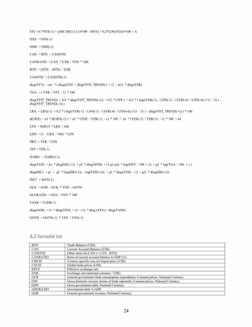
24

STI = 0.7*STI(-1) + ((HIC/HIC(-1)-1)*100 – INFT) + 0.2*LOG(YGA)*100 + A OXS = OXS(-1) OMS = OMS(-1) CAN = BTN + CANOTH CANRATIO = CAN * EXR / YEN * 100. BTN = (XTN - MTN) / EXR CANOTH = CANOTH(-1) dlog(YFT) = m1 * ( dlog(LFN) + dlog(YFIT_TREND) ) + (1 - m1) * dlog(XTR) YGA = ( YER / YFT - 1) * 100 dlog(YFIT_TREND) = 0.8 * dlog(YFIT_TREND(-1)) + 0.2 * (TFP ) + 0.2 * ( log((YER(-1) / LNN(-1) / (YER(-4) / LNN(-4)) )^(1 / 3) ) - dlog(YFIT_TREND(-1)) ) LRX = LRX(-1) + 0.2 * ( log((YER(-1) / LNN(-1) / (YER(-4) / LNN(-4)) )^(1 / 3) ) - dlog(YFIT_TREND(-1)) ) * 100 d(URX) = n1 * d(URX(-1) ) + n2 * (YER / YER(-1) - 1) * 100 + n3 * (YER(-2) / YER(-3) - 1) * 100 + n4 LFN = POP15 * LRX / 100 LNN = (1 - URX / 100) * LFN PRO = YER / LNN TFP = TFP(-1) NAIRU = NAIRU(-1) dlog(YED) = p1 * dlog(HIC(-1)) + p2 * dlog(MTD) + (1-p1-p2) * log(INFT / 100 + 1) + p3 * log(YGA / 100 + 1 ) dlog(HIC) = q1 + q2 * (log(HIC(-1)) - log(YED(-1))) + q3 * dlog(YED) + (1 - q3) * dlog(HIC(-1)) INFT = INFT(-1) GLN = GGR - GCR * YED - GOTH GLNRATIO = GLN / YEN * 100. TAXR = TAXR(-1) dlog(GGR) = r1 * dlog(YEN) + (1 - r1) * dlog (XTN) + dlog(TAXR) GOTH = GOTH(-1) * YEN / YEN(-1)

A.2 Variable list

BTN Trade Balance (US$)

CAN Current Account Balance (US$)

CANOTH Other items for CAN (= CAN - BTN)

CANRATIO Ratio of current account balance to GDP (%)

CMUD Country-specific non-oil import price (US$)

CXUD Global trade prices (US$)

EFEX Effective exchange rate

EXR Exchange rate (national currency / US$)

GCR General government final consumption expenditure, Constant prices, National Currency

GDI Gross domestic income (terms of trade adjusted), Constant prices, National Currency

GDN Gross government debt, National Currency

GDNRATIO Government debt % GDP

GGR General government revenue, National Currency

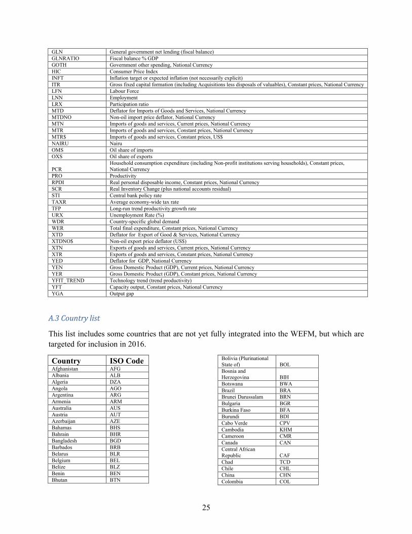
25

GLN General government net lending (fiscal balance)

GLNRATIO Fiscal balance % GDP

GOTH Government other spending, National Currency

HIC Consumer Price Index

INFT Inflation target or expected inflation (not necessarily explicit)

ITR Gross fixed capital formation (including Acquisitions less disposals of valuables), Constant prices, National Currency

LFN Labour Force

LNN Employment

LRX Participation ratio

MTD Deflator for Imports of Goods and Services, National Currency

MTDNO Non-oil import price deflator, National Currency

MTN Imports of goods and services, Current prices, National Currency

MTR Imports of goods and services, Constant prices, National Currency

MTR$ Imports of goods and services, Constant prices, US$

NAIRU Nairu

OMS Oil share of imports

OXS Oil share of exports

PCR Household consumption expenditure (including Non-profit institutions serving households), Constant prices, National Currency

PRO Productivity

RPDI Real personal disposable income, Constant prices, National Currency

SCR Real Inventory Change (plus national accounts residual)

STI Central bank policy rate

TAXR Average economy-wide tax rate

TFP Long-run trend productivity growth rate

URX Unemployment Rate (%)

WDR Country-specific global demand

WER Total final expenditure, Constant prices, National Currency

XTD Deflator for Export of Good & Services, National Currency

XTDNO$ Non-oil export price deflator (US$)

XTN Exports of goods and services, Current prices, National Currency

XTR Exports of goods and services, Constant prices, National Currency

YED Deflator for GDP, National Currency

YEN Gross Domestic Product (GDP), Current prices, National Currency

YER Gross Domestic Product (GDP), Constant prices, National Currency

YFIT_TREND Technology trend (trend productivity)

YFT Capacity output, Constant prices, National Currency

YGA Output gap

A.3 Country list

This list includes some countries that are not yet fully integrated into the WEFM, but which are

targeted for inclusion in 2016.

Country ISO Code Afghanistan AFG

Albania ALB

Algeria DZA

Angola AGO

Argentina ARG

Armenia ARM

Australia AUS

Austria AUT

Azerbaijan AZE

Bahamas BHS

Bahrain BHR

Bangladesh BGD

Barbados BRB

Belarus BLR

Belgium BEL

Belize BLZ

Benin BEN

Bhutan BTN

Bolivia (Plurinational State of) BOL

Bosnia and Herzegovina BIH

Botswana BWA

Brazil BRA

Brunei Darussalam BRN

Bulgaria BGR

Burkina Faso BFA

Burundi BDI

Cabo Verde CPV

Cambodia KHM

Cameroon CMR

Canada CAN

Central African Republic CAF

Chad TCD

Chile CHL

China CHN

Colombia COL

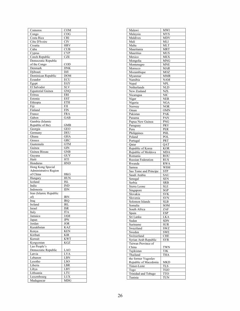
26

Comoros COM

Congo COG

Costa Rica CRI

Côte D'Ivoire CIV

Croatia HRV

Cuba CUB

Cyprus CYP

Czech Republic CZE

Democratic Republic of the Congo COD

Denmark DNK

Djibouti DJI

Dominican Republic DOM

Ecuador ECU

Egypt EGY

El Salvador SLV

Equatorial Guinea GNQ

Eritrea ERI

Estonia EST

Ethiopia ETH

Fiji FJI

Finland FIN

France FRA

Gabon GAB

Gambia (Islamic Republic of the) GMB

Georgia GEO

Germany DEU

Ghana GHA

Greece GRC

Guatemala GTM

Guinea GIN

Guinea Bissau GNB

Guyana GUY

Haiti HTI

Honduras HND

Hong Kong Special Administrative Region of China HKG

Hungary HUN

Iceland ISL

India IND

Indonesia IDN

Iran (Islamic Republic of) IRN

Iraq IRQ

Ireland IRL

Israel ISR

Italy ITA

Jamaica JAM

Japan JPN

Jordan JOR

Kazakhstan KAZ

Kenya KEN

Kiribati KIR

Kuwait KWT

Kyrgyzstan KGZ

Lao People’s Democratic Republic LAO

Latvia LVA

Lebanon LBN

Lesotho LSO

Liberia LBR

Libya LBY

Lithuania LTU

Luxembourg LUX

Madagascar MDG

Malawi MWI

Malaysia MYS

Maldives MDV

Mali MLI

Malta MLT

Mauritania MRT

Mauritius MUS

Mexico MEX

Mongolia MNG

Montenegro MNE

Morocco MAR

Mozambique MOZ

Myanmar MMR

Namibia NAM

Nepal NPL

Netherlands NLD

New Zealand NZL

Nicaragua NIC

Niger NER

Nigeria NGA

Norway NOR

Oman OMN

Pakistan PAK

Panama PAN

Papua New Guinea PNG

Paraguay PRY

Peru PER

Philippines PHL

Poland POL

Portugal PRT

Qatar QAT

Republic of Korea KOR

Republic of Moldova MDA

Romania ROU

Russian Federation RUS

Rwanda RWA

Samoa WSM

Sao Tome and Principe STP

Saudi Arabia SAU

Senegal SEN

Serbia SRB

Sierra Leone SLE

Singapore SGP

Slovakia SVK

Slovenia SVN

Solomon Islands SLB

Somalia SOM

South Africa ZAF

Spain ESP

Sri Lanka LKA

Sudan SDN

Suriname SUR

Swaziland SWZ

Sweden SWE

Switzerland CHE

Syrian Arab Republic SYR

Taiwan Province of China TWN

Tajikistan TJK

Thailand THA

the former Yugoslav Republic of Macedonia MKD

Timor-Leste TLS

Togo TGO

Trinidad and Tobago TTO

Tunisia TUN

27

Turkey TUR

Turkmenistan TKM

Uganda UGA

Ukraine UKR

United Arab Emirates ARE

United Kingdom of Great Britain and Northern Ireland GBR

United Republic of TZA

Tanzania

United States of America USA

Uruguay URY

Uzbekistan UZB

Vanuatu VUT

Venezuela, Bolivarian Republic of VEN

Viet Nam VNM