World Development abstract - 千葉大学園芸学部 · Gonzalez, all of the Ministry of Planning and Economic Policy (MIPPE) of Panama, and two anonymous referees as well as the

FHPANA14.DOC

The Poverty and Heterogeneity among Female Headed Households Revisited:

The Case of Panama∗∗∗∗

by

Nobuhiko Fuwa,

Chiba University, 648 Matsudo,

Matsudo-City, Chiba, 271-8510 Japan

[email protected]

Fax: 81-47-308-8932

October, 1999

(forthcoming in World Development)

abstract

Investigating whether female headed households (FHHs) are particularly disadvantaged

requires more systematic ways of poverty comparisons than typically found in the past. In

Panama, while FHHs as a whole appear to be better-off on average, such results are

somewhat sensitive to assumptions about economies of scale in household consumption,

and more disaggregated analysis reveals that particular segments of FHHs, particularly self-

reported FHHs with common-law partners living in urban areas, are disadvantaged in both

consumption and some non-consumption dimensions. Thus less systematic analysis could

fail to identify such ‘pockets of poverty’ that might deserve special policy attention.

JEL Classification: J12, J16, O18, O54

Key words: female-headed households, poverty, gender, Latin America, Panama.

∗ This paper was initially written while the author was on the staff of the World Bank. He would like to thank especially Kathy Lindert and Carlos Sobrado for valuable assistance and very useful discussions.

He would also like to thank Rosa Elena de De la Cruz, Edith Kowalzyk, Eudemia Perez, and Roberto

Gonzalez, all of the Ministry of Planning and Economic Policy (MIPPE) of Panama, and two

anonymous referees as well as the editor for very useful comments. The views expressed in this paper

do not represent those of the World Bank.

1

The Poverty and Heterogeneity among Female Headed Households Revisited:

The Case of Panama

1. INTRODUCTION

While policy discussion regarding female headed households (FHHs) is not new, it is

still a controversial issue. As household-level data sets became increasingly available in many

developing countries validity of some of the empirical regularities earlier claimed, such as the

higher poverty among FHHs, have been somewhat questionedi, conventional definitions of

‘household headship’ have been criticizedii and policy implications have been debatediii. In this

paper, we conduct an analysis of FHHs based on the 1997 Panama Living Standard Measurement

Study data focusing on one of the central questions of the female headship analysis: Are female

headed households proportionately over-represented among the poor, and can female headship be

an appropriate targeting criterion for poverty focused policy interventions?

We will argue that in addressing this question we need more systematic ways of poverty

comparisons between FHHs and non-FHHs than typically conducted in the past. Such analysis

should include sensitivity analyses incorporating some methodological aspects of comparisons in

consumption poverty and alternative headship definitions. It should also include non-

consumption dimensions of poverty. Our findings from Panama show that the answer to the

above question depends on the further disaggregation of various sub-types of FHHs, adjustments

of per-capita household expenditure measures in terms of demographic composition of the

household, and geographical disaggregation within Panama. We find, in particular, that while the

(self-reported) FHHs as a whole appear to be better-off than their male headed counterparts on

2

average, such results are somewhat sensitive to the incorporation of economies of scale in

household consumption, and, furthermore, more disaggregated analysis reveals that a particular

segment of FHHs, the self-reported FHHs who have common-law partners living in urban areas,

are at a great disadvantage in both consumption and some non-consumption dimensions of

poverty. The use of less systematic analysis could fail to identify such vulnerable groups who

might potentially deserve special policy attention.

2. THE POVERTY OF FHHS REVISITED: A REVIEW OF RECENT LITERATURE

A large number of empirical studies have been conducted on the relationship between

female headship and poverty, measured by household consumption or income, in developing

countries. In general, as a few recent reviews have concluded,iv female headship is often found

to be associated with higher incidence of poverty. For example, Buvinic and Gupta (1997)

reviewed 61 studies examining the relationship between female headship and poverty; 38 studies

found that FHHs were over-represented among the poor, additional 15 studies found associations

between poverty and some types of female headship, and only eight studies found no evidence of

greater poverty among FHHs. Most of the studies are based on the “self-reported” headship

definitions although a few had further disaggregation such as de facto or de jure FHHsv. Based

on these findings, they argue that “headship should seriously be considered as a potentially useful

criterion for targeting antipoverty interventions, especially in developing countries where means

testing is not feasible.” On the other hand, however, a recently conducted analysis by

Quisumbing, et al. (1995), using household survey data sets from 10 developing countries, find

that while poverty measures among FHHsvi tend to be higher in the majority of their sample

3

countries (7 out of 10), in a third to a half of them statistically significant, such evidence may not

be necessarily robust; in particular, their analysis using stochastic dominance tests reveals that it

is only in two countries (rural Ghana and Bangladesh) out of the ten where FHHs have

consistently higher poverty among the bottom third of population. Their general conclusion thus

is that “differences between male- and female-headed households among the very poor are not

sufficiently large that one can conclude that one is unambiguously worse- or better-off.”vii

While it is difficult to draw any systematic conclusions from these studies with rather different

findings,viii at least the latter study casts some doubts about the robustness of the often claimed

association between the general female headship and higher poverty.

One of the main reasons behind such seemingly contradicting conclusions appears to be

the fact that FHHs constitute a heterogeneous group of households with different types of FHHs

with different reasons for becoming female headed. Thus the compositions of different types of

FHHs are likely to be different across countries and across different areas within countries.

Generally, detailed country studies tend to suggest that the relationships between female headship

and poverty could differ significantly depending on the further disaggregation of reported

headship by marital status and other demographic characteristics, or on alternative headship

definitions.ix Dréze and Srinivasan (1998), for example, focus on the poverty of widow-headed

households, who are found to be more disadvantaged than the more general categories of FHHs.

A few studies employed alternative ‘economic’ definitions of female headship; while

Rosenhouse (1989) finds that use of her ‘working head’ definition identifies stronger positive

relation between female headship and greater poverty compared to the self-reported headship in

4

Peru, Rogers (1995), with an ‘economic definition’ of headship in terms of earned income, as

well as Handa (1994) with the ‘working headship’ definition, arrives at an opposite conclusion in

Dominican Republic and in Jamaica, respectively. Furthermore, as Buvinic and Gupta’s review

also points out, even within the same subtype of FHHs the likelihood of such households being

poor differs depending on specific country situations.

In addition to the large heterogeneity among FHHs, there are also methodological issues

involved in the analysis of household expenditure data that could affect the conclusions drawn

regarding the association between female headship and poverty. One of such issues is the

adjustment of per-capita consumption expenditure measures with adult-equivalence scales and

economies of scale. Such adjustments could potentially lead to significantly different policy

implications when, as is often the case, there are systematic correlations between female

headship, on the one hand, and household composition and household size, on the other. Also of

potential importance is the sensitivity of the female headship-poverty relationship with respect to

alternative poverty measures and poverty lines. For example, both Dréze and Srinivasan (1998)

in India and Bhushan and Chao (n.d.) in Ghana find that ignoring economies of scale would

underestimate the poverty of FHHs enough to lead to ‘rank reversals’ while ignoring adult

equivalent scales has relatively small quantitative effects. Louat et al.(1992), on the other hand,

find relatively large effects of adult equivalence adjustments as well as of using alternative

poverty measures. Quisumbing et al.(1995) find that whether or not FHHs are over-represented

among the poor somewhat depends on the level of the poverty line, while Dréze and Srinivasan

(1998)’s results were found to be robust across a wide range of poverty lines.

5

Therefore, despite the conclusions drawn by some observers, many (though with some

exceptions, as noted above) past studies on the relationships between female headship and

poverty were likely to be clouded by many factors, including the ambiguity in the definition of

the headship concept in data, lack of distinction among very different types of female headship

situations and among potentially different regional contexts within countries, and possible

sensitivity of findings to alternative adjustment methods in incorporating household

demographics into household expenditure (or income) measures. In order to obtain policy

implications, such as the relevance of the female headship as a criterion for targeted anti-poverty

interventions, we need to understand systematic relationships between different types of female

headed households and poverty under different circumstances, which in turn will require more

systematic analyses than generally conducted in the past, incorporating all of these factors

mentioned above for each country. None of these past studies appears to have incorporated the

combination of all of these possible dimensions of sensitivity analyses simultaneously. Our

analysis of the Panamanian case is intended as an attempt in such a direction.

In addition, there are many non-income dimensions of poverty that need to be examined

in order to obtain a fuller picture of the poverty of FHHs. Above all, the issues that have drawn

particularly high attention are the ‘time poverty’ aspects of FHHs and intergenerational

transmission of disadvantages of FHHs, mainly through the nutritional status and education of

children. Because of the ‘double day burden’ on the female heads of economic support and

household chores, it is often argued, female heads are more likely to be ‘time poor’ (that is,

consume smaller amount of leisure time), than female or male heads of jointly-headed

6

households. Studies based on a few (though often incomplete) data sets do seem to suggest that

female heads of households tend to consume smaller amount of leisure.x

Furthermore, such “substitution of work for leisure to achieve a certain level of

consumption in female-headed households may signify the perpetuation of poverty into the next

generation,” (Buvinic and Gupta 1997). The issue of the possibility of intergenerational

transmission of disadvantages in FHHs is rather complicated, since there are at least two

counteracting forces in operation here. On one hand, if FHHs indeed tend to be poorer than non-

FHHs in terms of income, then it implies that children’s welfare may be lower in FHHs, through

lower consumption (including food consumption), lower education expenditures, and so on.

Furthermore, the ‘double day’ burden on the female heads could potentially place burden on

children’s time by forcing them to supplement or substitute their mothers’ work, thereby leading

to possibly less time for own education. On the other hand, however, there has been some

evidence that women tend to allocate greater shares of household resources toward their children

than men do, cetris paribus.xi If so, children within FHHs, presumably benefiting from such

stronger preferences of the female head toward children, might be better-off than their

counterpart in non-FHHs with same levels of income, because of the systematic differences in

the patterns of household resource allocation as a result of differential preferences between

women and men. Which of these counteracting forces tends to dominate is an empirical

question. It is thus not surprising that we find mixed results from empirical studies regarding the

positive or negative association between female headship and the welfare of children. For

example, Buvinic and Gupta (1997)’s review finds that among the 29 studies they covered there

7

was “a slight bias toward finding more protective effects in Africa, but recent studies report this

phenomenon also in Latin America and the Caribbean” (italic added) when the poverty outcomes

are measured by nutritional status and educational outcomes of children.

3. PANAMANIAN CONTEXTS AND THE DATA

As of 1997, Panama had a per capita GDP of US$3,080 with over two million people.

The 1997 Living Standard Measurement Study (LSMS) survey, conducted by the Ministry of

Planning and Economic Policy (MIPPE), indicates that the nationwide headcount poverty ratio in

1997 was 0.37, that its income inequality was among world’s highest with Gini coefficient of

0.6xii, and that the headcount poverty ratio had fallen between 1983 and 1997. (World Bank

1999) In analyzing the poverty of FHHs measured by consumption expenditures, we will use the

poverty line calculated by the World Bank; it is based on the minimum per-capita average daily

caloric requirement of 2,280 plus a specific level of allowance for non-food items (33%) which

is based on the actual expenditures by the households whose consumption expenditures are

around the level of the minimum caloric requirement. The annual per capita expenditure at the

poverty line thus derived is B$905.xiii

In Panama, gender disparity does not appear to be as pressing an issue as in some other

parts of the world, such as in South Asia. For example, on average years of schooling is higher

among girls than among boys (the reverse is true in indigenous areas, however). There is no

evidence of gender bias against girls in child nutrition, nor is there evidence of gender

discrimination in earnings after controlling for education and other observed characteristics. At

the same time, however, there is some evidence that unemployment rate is higher among women,

8

that gender barriers exist in terms of sector of employment and of promotion within firms, that

rural women are more constrained than men in access to credit and extension services, and that

domestic violence could be a serious problem.xiv

There appears to be an increasing trend in the proportion of FHHs in many countries

including Panama. (Buvunic and Gupta 1997) Regarding the poverty of FHHs in Panama, the

only previous study known to the present author is the one by Sahota (1990) based on the

National Socioeconomic Survey in 1983; it found that the general female headship was

associated with lower consumption expenditure and higher poverty in the context of multiple

regression analysis. On the other hand, more recent set of studies in Latin America (not

including Panama), all based on data in the mid 1990s, indicates that FHHs are not necessarily

overrepresented among the poor; among the 14 Latin American counries under study only in six

of them were FHHs overrepresented among the poor.xv

In the rest of the paper, we will examine the poverty of FHHs in Panama using the 1997

LSMS. The interviews were conducted during the period between July and September of 1997.

The total sample of households with completed questionnaires was 4,938 (representing 650,726

population households nationwide) containing 21,410 individuals (representing the population of

2,732,316 individuals nation wide), and is nationally representative for four geographic areas:

urban, rural indigenous, rural remote access and rural non-indigenous.xvi Here an ‘urban’ area is

defined as any area with more than 1,500 persons per kilometer.xvii

In our analysis of FHHs we will follow the geographical disaggregation among urban

(representing 56% of total population), rural (35%) and indigenous areas (9%), as adopted by the

9

LSMS sampling, since dynamics of becoming FHHs and possible disadvantages among FHHs

could potentially be different among these groups. In general, there may be relatively more

economic opportunities and less social constraints on women in urban than in rural areas. Such

factors in urban areas, in turn, may affect (weaken) the stability of marriage and may also affect

(increase) the prevalence of un-married relationships, thereby affecting the prevalence of female

headship in general. (e. g., Chant 1997: 93) Furthermore, Panama is often characterized by its

highly dualistic development pattern with its major cities (such as Panama City and Colon)

hosting the “internationally-oriented, modern, dynamic service ‘enclaves,’” suggesting

potentially very sharp urban-rural differences.xviii We can observe that both female labor force

participation and the share of FHHs are higher in urban than in rural areas. In addition, the rural-

urban disaggregation could be also appropriate given the way some sub-categories of FHHs may

arise in each area; for example, rural-urban migration of male household heads creates de facto

FHHs (to be defined below) in rural areas which may be economically supported by the

remittances from their husbands working in urban areas while such migration could potentially

induce de jure FHHs in urban areas if such migrants engage in extra-marital relationships in their

destinations. Furthermore, while there might be more economic opportunities for women in

urban areas, the level of social capital, arguably a major asset among the poor, appears to be

much lower in urban areas than in rural areas. (Pena and Lindo-Fuentes 1998)

In Panama, its major indigenous population has historically been concentrated in certain

geographical regions although smaller number of them live in all of Panama’s provinces. These

indigenous people live in rural settings, mainly engaged in agriculture, and their labor is

10

organized by sex and age.xix Although such characteristics may be similar to other (non-

indigenous) rural areas, indigenous areas are characterized by very low productivity and

extremely high (i. e., much higher than the other rural areas, as we will see later) incidence of

poverty. In addition, in contrast with non-indigenous areas, there is a gender gap in education

among children in indigenous areas. Also indigenous people appear to face discrimination in

labor market, such as lower earnings after controlling for education and other worker

characteristics. (World Bank 1999) At the same time, however, measures of ‘social capital’ in

indigenous areas tend to be higher than urban or non-indigenous rural areas, and there is some

indication that higher social capital may provide more possibilities for women to ‘realize their

potential.’ (Pena and Lindo-Fuentes 1998) It appears that these various differences among urban,

rural and indigenous areas could potentially affect the poverty outcomes among FHHs in

different ways.

4. SHARES OF FHHS WITH ALTERNATIVE HEADSHIP DEFINITIONS

Before looking into the poverty of FHHs in Panama using alternative headship

definitions, we will briefly examine the question: to what extent do different definitions of FHHs

identify different sets of households as female headed? As we can see from Table 1, at the

national aggregate level, self-reported female headed households represent a little less than one

quarter (22%) of the total households. FHHs tend to have a higher share in urban area (28%) and

lower shares in rural and indigenous areas (17% and 15%, respectively). Table 2 shows the

degree to which alternative definitions of FHHs identify different sets of households as female

headed. If the households identified as FHHs by alternative definitions do not vary much then

11

applying alternative definitions in analyzing the poverty of FHHs would be of little value. In our

analysis, we will differentiate seven sub-categories of self-reported FHHs: 1. de jure FHHs (i. e.,

those self-reported FHHs where the reported head is either unmarried/single, divorced/separated,

or widowed), further disaggregation of de jure FHHs according to the head’s marrital status (i. e.,

2. unmarried, 3. divorced or separated, and 4. widowed), 5. self-reported FHHs who have

spouses (‘casada’), 6. self-reported FHHs who have unmarried/common-law male partners

(‘unida’), and 7. de facto FHHs (i. e., those self-reported FHHs where the reported head has her

spouse or common-law male partner but they are not physically presentxx). In addition, we will

also use three alternative (non-self reported) definitions of FHHs. Such alternative definitions of

FHHs include what can be called a purely demographic definition and economic definitions. For

the former, we will use ‘Potential FHHs’ (i. e., those households where there is no working age

male –defined as between age 15 and 60– is present). The ‘potential FHH’ definition of FHHs

has been used when analyzing a data set containing demographic compositions but not economic

activities, such as in censuses.xxi For the ‘economic definition’ of FHHs, which signifies the

aspect that the main economic supporter of the household is female rather than male, we follow

Rosenhouse (1989)’s definition of the ‘working head’; we identify the household member who

contributed more than 50% of the total hours of work (including paid labor market hours, unpaid

hours on farm and on family enterprises, but excluding household chores or child care) by all the

household members combined during the week preceding the survey interview and ‘working’

FHHs are identified as those households where such main labor-hour contributor is a woman.

Finally, we take a look at the intersection of both economic and demographic definitions of

12

household headship. For that purpose, we identify those FHHs, what we might call ‘Core

FHHs,’ which qualify as female headed by both the ‘working head’ definition and the ‘potential

FHH’ definition of female headship –this should identify the households that conceptually fit the

prototypical notion of FHHs: i. e., the absence of any steady male partner and the female being

the primary economic supporter of the household.

As we can see in Table 2, the households identified as FHHs do differ significantly

depending on which definition of household headship is adopted. In most of the cases the

overlap appears typically around 40 to 60%. For example, among the self-reported FHHs, only

about 40% of them are also classified as female headed with the ‘working head’ definition while

50% of them also qualify as ‘potential FHHs’ (see the first column of Table 2). This seems to

indicate that the degree of economic support is not as strong a factor as demographic composition

in self-reported headship in Panama; this appears consistent with the view that women’s

economic contribution is often under-recognized in the self-definition of the headship, compared

to other factors such as age, asset ownership and the conventionally assumed role (or norm) of

male authority. Conversely, among the FHHs defined by the ‘working head’ definition, only

57% are also self-reported as FHHs and 48% are also classified as ‘potential FHHs.’ (last column

of Table 2).

(TABLE 1 AND 2 AROUND HERE)

5. CONSUMPTION POVERTY OF FHHS IN PANAMA

(a) Headcount poverty ratios by alternative female headship definitions

Table 3 reports the headcount poverty ratios, applied to per capita household

13

expenditures, of FHHs versus the rest of the households. At the national aggregate level, there is

no evidence that FHHs, whether self-reported (without any further breakdown), or by purely

demographic or economic (‘working head’) definition, are more likely to be poor than non-

FHHs. It appears that the opposite is true; the headcount poverty ratio among self-reported FHHs

is 29% while that of self-reported ‘male headed’ households is 40% and the difference is

statistically significant.

(TABLE 3 AROUND HERE)

Given the large heterogeneity among FHHs, however, more appropriate question would

be: what type of FHHs, if any, are over-represented among the poor and thus worthy of special

policy attention? Once we start disaggregating self-reported FHHs by marital status, we find

slightly more subtle patterns. For example, among some sub-groups of the self-reported FHHs,

while those with legally married spouses (casada) do not have higher headcount poverty ratios in

any of the area, the self-reported FHHs with common-law partners (‘unida’ category) have

significantly higher headcount poverty ratios nation-wide, in urban and in indigenous areas.

Such households are, however, a very small minority. We can also further disaggregate de jure

FHHs among those headed by widows, by separated or divorced, and by single women. De jure

FHHs headed by widows and by divorced or separated women have significantly higher

headcount poverty ratios in indigenous areas but not in any other area. What really stands out in

indigenous areas, however, is the overwhelmingly high incidence of poverty in indigenous areas,

with mostly over 90% poor. In such a situation, gender of headship is not quite an issue since

virtually every one is poor in most cases.xxii In fact, disaggregated analysis of the male-headed

14

households (not reported) reveals that there is no significant difference in the headcount poverty

ratios between FHHs and male headed households in any of the disaggregated categories of

headship in indigenous areas.

Now departing from the self-reported female headship definition, we turn to the

headship analysis using the purely demographic and ‘economic’ definitions. We find again that

these FHHs are significantly less likely to be in poverty than are the rest of the households. Our

results present a sharp contrast with Rosenhouse (1989)’s findings from Peru where FHHs

defined in terms of ‘working head’ tended to have higher headcount poverty ratios than self-

reported FHHs, and are more in line with Rogers (1995)’ findings from Dominican Republic and

Handa (1995)’s from Jamaica that the use of ‘economic’ headship definitions, rather than that of

self-reported headship, tends to make FHHs appear economically better off. Finally, the ‘core’

FHH categories also turn out to be less likely to be poor than non-FHH.xxiii

Such somewhat mixed patterns seem to suggest that the dynamics of becoming female

heads of households and the reasons why particular sub-categories of FHHs may be poorer differ

among urban, rural and indigenous areas. The higher poverty among FHHs with unmarried

partners (unida) in urban areas, for example, might be due to the much greater economic

opportunities for women which enable them to sustain FHHs and, in addition, to the existence of

multiple female partners of some Panamanian men that is much more prevalent in urban than in

other areas.xxiv In some parts of the world, such as in South Asia, widows have long been

recognized as being particularly disadvantaged and poor;xxv in Panama, however, there is not an

indication that widows are disadvantaged, in terms of consumption poverty, in non-indigenous

15

rural areas.

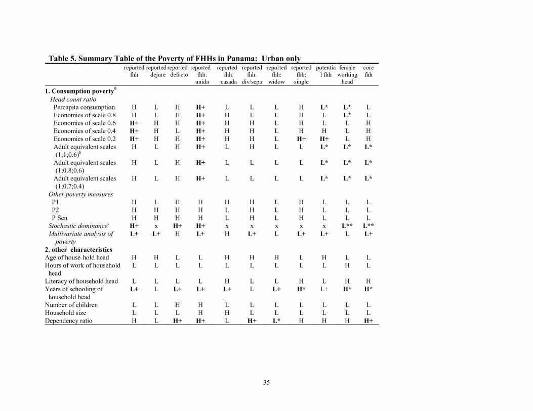
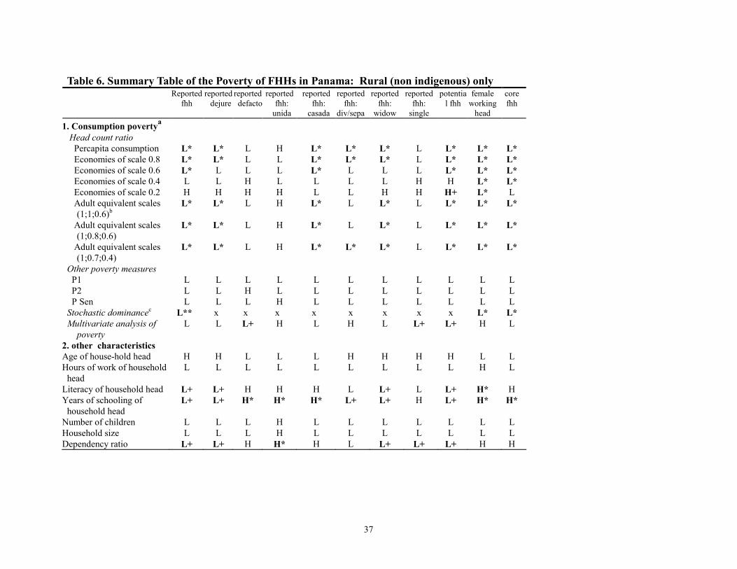
(TABLE 4, 5, 6 AND 7 AROUND HERE)

(b) Headcount poverty ratios with adult equivalence and economies of scale taken into account

In our analysis above, we have used per capita consumption expenditures as the

indicator of the welfare level of the household. There are at least two additional considerations

as to how, in theory, a consumption measure of household welfare could better incorporate

differences in demographic composition of the households than the simple per capita measure:

adult equivalence scales and economies of scale. Since the consumption needs of children may

be met at lower cost than those of adults, the per capita consumption measure could understate

(overstate) the welfare level of the households with larger (smaller) proportion of children, given

the same total number of household members. Furthermore, if economies of scale exist in

household consumption, then the per capita consumption measure could understate (overstate)

the welfare level of larger (smaller) households given the same level of per capita consumption

level. We conduct sensitivity analyses using a range of alternative parameter values that appear

plausible for both adult equivalence scales and the economies of scale in household consumption.

In general, if there are systematic differences in the household size and household composition

(especially in terms of the proportion of children among the household members) between female

headed and non-female headed households, then the welfare level would be systematically under-

or over-stated between these two categories.

Our data from Panama show that the proportion of children among household members

16

tends to be smaller in self-reported FHHs than in non-FHHs. The average number of children

(age 15 or below) among self-reported FHHs, for example, is 1.19 while that among non-FHH is

1.69, and average shares of children of age 15 or below in the total number of household

members are 24% among self-reported FHHs and 29% among non-FHHs. Thus incorporating

adult equivalence scales could potentially increase the estimated headcount poverty ratios among

FHHs. Tables 4 through 7 summarize qualitative results of various sensitivity and other analyses

of poverty of FHHs to be discussed in the rest of the paper. xxvi It turns out that incorporating

adult equivalent scales has very small quantitative effects on estimates of headcount poverty

ratios and thus has virtually no effect on qualitative conclusions obtained from the estimates

using simple per capita measuresxxvii.

Since female headed households often tend to be of smaller size than non-female headed

households, some recent studies have found that the difference in headcount poverty ratios

between female headed and male headed households is sensitive to the assumption about the

degree of economies of scale in household consumption,xxviii and that incorporating the

economies of scale assumption tends to increase the headcount poverty ratios among FHHs. In

our Panamanian data, the average household size among self-reported FHHs is 3.7, while that

among self-reported male headed households is 4.5. Following Lanjouw and Ravallion (1995),

we use the economies-of-scale-adjusted per-capita consumption expenditures (xi) defined as:

xX

ni

i

i

≡ θ ,

where Xi is the total household consumption expenditure for household i, ni is the household size

and O is the ‘size elasticity’ measuring the degree of economies of scale in household

17

consumption, varying between 0 and 1 (where the smaller the O becomes within the range the

higher is the degree of economies of scale, with the O value of 1 representing no economies of

scale –thus xi reduces to per capita expenditure – and value 0 representing a situation where all

household consumption has public good property –xi equals total household expenditure – xxix; in

our analysis we used values between 1.0 and 0.2).xxx We find that the point estimates of

headcount poverty ratios are somewhat sensitive to the economies of scale assumptions.

Generally as the value of O decreases we tend to observe an increasing number of ‘rank reversal’

where the headcount poverty ratios of FHHs become higher than those of non-FHHs. However,

many of such changes tend not to be statistically significant. This makes it difficult to draw

unambiguous conclusions about poverty comparisons in many instances.

(c) Sensitivity to alternative poverty measures and alternative poverty lines

So far we have focused on the headcount poverty ratios, and thus have not taken into

account the degree or depth of poverty. In order to examine the sensitivity of above findings

when distribution among the poor is taken into account, we apply a few alternative poverty

measures to poverty comparisons between FHHs and the rest of the households; alternative

measures used here are the poverty gap (P1), Foster-Greer-Thorbecke measure (FGT) with its ‘O’

parameter equal to two (P2), and Amartya Sen’s measure (PSen).xxxi Our results show, as

summarized in the 9th to 11th rows in Tables 4 through 7, that the patterns of poverty comparisons

between female headed versus non-female headed households do not change except for a

relatively small number of cases. In none of such cases is the initial difference in the headcount

poverty measures statistically significant and thus our overall observations from headcount

18

measures do not seem to be affected significantly by the use of alternative poverty measures that

take into account distribution among the poor.

Another aspect of sensitivity analysis in poverty comparisons concerns the level of the

poverty line. In order to examine the sensitivity of our findings above, we conducted first order

stochastic dominance test with B$2,000, which is roughly twice the poverty line used above, as

the upper bound. Using this analysis, if the poverty incidence curve of non-FHHs (FHHs) is

found to be first order stochastic dominant over that of FHHs (non-FHHs) within the range, then

the headcount poverty ratio of FHHs (non-FHHs) is always higher no matter what the level of the

poverty line is as far as it is below the upper bound. Our analysis shows (see the 12th rows in

Tables 4 through 7) that many of the poverty comparison results emerged in the previous sections

are somewhat sensitive to the specific level of the poverty line used, which is in line with

Quisumbing et al (1996)’s findings; in a majority of the cases the poverty incidence curve of

neither FHHs nor non-FHHs dominates that of the other. Nevertheless, at the national aggregate

level, roughly half of the cases where FHHs are found to be better-off earlier turn out to be robust

regardless of the poverty line while in urban areas a few cases (including that of unida-FHHs)

with higher poverty among FHHs are also found to be robust.

(d) Multivariate analysis of the consumption poverty of FHHs

There appears to be some systematic correlation between female headship and some

dimensions of household characteristics. Thus, the bivariate poverty comparisons we have

conducted so far may potentially reflect the results of not so much the poverty (or non-poverty)

of FHHs per se as that of the households with particular household characteristics such as small

19

household size. In order to examine whether female headship is associated with higher or lower

poverty after controlling for other household characteristics, we regressed per-capita household

expenditures on a set of household characteristics, including a dummy variable for female headed

householdsxxxii. The estimated coefficients on the female headship dummies, using alternative

definitions of female headship, are summarized in Table 8, and coefficient estimates of the other

control variables are presented in Appendix Table 1.xxxiii As we saw earlier, one key variable that

appears strongly associated with both female headship and poverty is the household size. So we

compared the association between female headship and household expenditure with and without

the household size variable included. We can see from Table 8 that results are affected by

whether or not the household size is controlled. When household size is not controlled for,

except in urban areas, female headship has either no statistical association or positive association

with per capita household expenditures, especially using purely demographic and ‘working-head’

definitions. However, once household size is controlled, such positive association completely

disappears. Instead, we can find a strong negative association between female headship and

household expenditures especially in urban areas, and, to some extent, in rural areas as well as at

the national aggregate. That female headship is negatively correlated with household

consumption expenditures after controlling for household characteristics is generally in line with

an earlier study by Sahota (1990) based on the 1983 data. We can conclude that the greater

economic disadvantages of FHHs, to the extent they exist, is mainly an urban phenomenon,

where, among many categories of FHHs, female headship is associated with possibility of higher

likelihood of poverty, after controlling for the household size, household composition and age

20

and education of the household head.

(TABLE 8 AROUND HERE)

6. INTERGENERATOINAL TRANSMISSION OF DISADVANTAGES?: SCHOOL

ENROLLMENT RATES OF CHILDREN

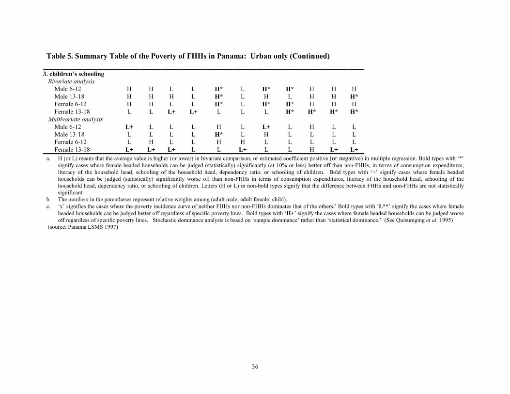
(a) Bivariate analysis

Welfare indicators of children could be particularly important information that is

complimentary to current household consumption level, because they suggest the possibility of

intergenerational transmission of poverty. When we examine the average proportion of

children enrolled in school within the household at the time of the survey with two separate age

groups (age 6 to 12 and age 13 to 18) of children by gender, the correlation between the gender of

household head and school enrollment of children is not overwhelming as a whole. To the extent

there is such correlation, however, at the primary schooling level (age 6 to 12) female headship is

generally correlated with higher rather than lower school enrollment of children. Thus

indications for the possibility of intergenerational transmission of poverty in FHHs, measured by

school enrollment of children at least, appear to be weak.

At the secondary schooling level (age 13 and 18), bivariate correlation between female

headship and school enrollment is even less clear than at the elementary level. At this level,

higher school enrollment of children, to the extent there is significant correlation, is mainly

correlated with ‘working head’ definitions of FHHs and purely demographic definitions of

FHHs, but not so much with the self-reported headship categories (with a few exceptions where

there are very small number of observations). In addition, unlike in the case of primary

21

schooling level, there are a few cases where school enrollment ratios are lower in FHH than in

non-FHHs. Thus, at the level of secondary schooling when children can be counted as labor

force, it appears that in some subcategories of self-reported FHHs, the time burden upon

children’s labor time is possibly so large as to reduce their school enrollment.

(b) Multivariate analysis

Like the case of consumption expenditure, we also conducted regression analysis in an

attempt to assess correlation between children’s schooling and female headship after controlling

for other household characteristics, such as age and education of the head, per capita household

expenditure, household size, household composition and regional dummies. Estimated

coefficients on alternative female headship dummiesxxxiv are summarized in Tables 9 and 10, and

more detailed regression results are reproduced in Appendix Tables 2 and 3.xxxv Among the

children of age 6 to 12, except in urban areas, there tends to be positive association between

female headship and higher primary school enrollment, especially in rural areas, after controlling

for other household characteristics. An exception to this tendency, however, appears to be the

case of urban boys where there is some negative association. Furthermore, as we saw in the

bivariate analysis above, the positive impact of the female headship on children’s school

enrollment, to the extent it exists, becomes much weaker at the secondary school level. Not only

are there fewer cases of positive association, but in the case of teenage girls in urban areas the

correlation between female headship and school enrollment is mostly negative with about half of

the female headship categories having statistically significant effects. Again, to the extent there

is substitution between mothers’ and children’s labor within FHHs, it occurs mostly at teenage

22

level, and, furthermore, female heads’ time use appears more highly substitutable with their

teenage girls’ time than with boys’ within the household resource allocation.

(TABLE 9 AND 10 AROUND HERE)

7. TRIPLE BURDEN?

There is a view that FHHs are at a greater economic disadvantage due to the “triple

burden;”xxxvi (1) the main income earner being female with various disadvantages in the labor

market and in other productive activities, (2) the ‘head’ being both the main earner and

responsible for maintaining the household, including household chores and child care, and thus

being ‘time poor,’ and (3) the ‘head’ often being the single earner (rather than joint) thus facing

higher dependency burden. Regarding the first aspect of such ‘triple burden,’ the earning

capacity of a household head partially depends on her or his human capital endowment. We can

see in Tables 4 through 7, that when headship is defined in terms of ‘working head,’ female

heads tend to have higher rather than lower education endowment, except in indigenous areas.

Among self-reported female heads, however, female heads do seem to have lower level of

education in indigenous areas in terms of literacy, and in mainly urban areas in terms of years of

schooling. In rural areas, it appears that it is only the female heads without any male partners

that have lower education.

Regarding the time burden on the female head of both economic support and household

maintenance activities, the second aspect of the ‘triple burden,’ except for the ‘working head’

FHHs and FHHs with male partners (with spouse or with common-law partner), female heads

indeed tend to work fewer hours than their male counterparts in urban and rural areas.xxxvii This

23

indicates the possibility that the household maintenance activities are the binding constraint on

their labor supply. In addition, from school enrollment of children we did not find much strong

evidence that children are mainly performing the household maintenance activities in place of

their mothers (at least to the extent that such activities become binding constraint on school

enrollment) with a possible exception of teenage girls in urban areas; sometimes female headship

appears correlated with higher school enrollment, particularly at the primary school level. This

again appears to suggest that female household heads are often bearing the ‘double day’ time

burden themselves.

Among the ‘triple burden’ as described above, the third aspect (i. e., the possibly higher

dependency burden) appears least compelling among FHHs in Panama. As summarized in

Tables 4 through 7, FHHs (with most of their alternative definitions) have both fewer children

and smaller total household size, and it is only a minority of cases where dependency ratios of

FHHs are significantly higher than those of non-FHHs. In a number of cases, dependency ratios

of FHHs are lower than those of non-FHHs. Furthermore, we find that all the cases of positive

bivariate correlation observed between female headship and lower poverty disappear once

household size is controlled for in the context of multiple regression. This suggests that many

subcategories of self-reported FHHs are indeed better off than non-FHHs despite the female

heads’ possibly lower earning capacities and the ‘double day’ time burden on female heads,

because, in contrast with the common assertion of the ‘triple burden,’ their dependency burden is

often lower than that of non-FHHs.

24

8. CONCLUSIONS

We find that self-reported FHHs as a whole are not over-represented among the poor in

Panama, but that FHHs are rather better-off on average than self-reported male headed

households. Therefore the broad category of ‘female headship’ is not a useful tool for targeting

interventions toward the poor. Furthermore, the familiar assertion of the “triple burden” of FHHs

is only partially true, at best, depending on the definitional and geographical disaggregation of

household headship.

Nevertheless, our study also indicates that detailed female headship analysis of

consumption and non-consumption dimensions of poverty, as well as of other household

characteristics, could still be used as a potentially useful starting point for identifying some

specific segments of disadvantaged or vulnerable population within the heterogeneous group of

FHHs. Our multivariate analysis shows that FHHs often tend to be poorer once household size

and other characteristics are controlled for. Furthermore, even within the context of bivariate

analyses, we find that some segments of FHHs are indeed disadvantaged, and that such

disadvantages of FHHs, to the extent they exist, appear to be largely (though not exclusively)

urban phenomena. In particular, urban FHHs with unmarried partners, unlike many other sub-

categories of FHHs, are particularly disadvantaged, although the number of such households is

quite small. In our analysis these households are found to be disadvantaged on both income and

non-income dimensions such as higher consumption poverty, household heads being relatively

less educated, and higher dependency burden with many children. Beyond that, however, our

analysis reveals relatively little about how they come to fall into this type of household headship

25

in the first place and why they tend to be poor. The main value of the kind of disaggregated

analysis as conducted in this paper would be not so much a tool for targeted interventions as a

starting point for a focused in-depth study, perhaps of a qualitative approach, which in turn could

inform policy makers in terms of policy measures for addressing the poverty of such groups.

Also potentially disadvantaged are FHHs headed by widows in indigenous areas.

However, as far as indigenous areas are concerned, more important is the overwhelming

prevalence of poverty in the area as a whole, so much so that gender of headship is not an issue –

almost everyone is poor. Our study reveals that disaggregated FHH analysis could be a

potentially useful first cut at the effort of identifying the poor in some circumstances, but that it is

also only one of many possible ‘cuts,’ some of which can be more important than the gender of

headship, in other circumstances.

NOTES

i For example, see Quisumbing, et al. (1995) and Louat, et al, (1992).

ii See Rosenhouse (1989). iii See, for example, Buvinic and Gupta (1997) and Bruce and Lloyd (1997). iv Buvinic and Gupta (1997) and Haddad, et al. (1996). v As has been frequently pointed out, in a great majority of studies, the “female household heads” are self-

identified by survey respondents without clear a priori definition of household headship given in the survey.

This ambiguity in the meaning of FHHs found in surveys has been one of the major difficulties for the analysis

of FHHs. One approach to address this ambiguity has been to disaggregate self-reported household headship

into subsets, such as de facto and de jure FHHs. An alternative approach has been to completely depart from

the self-reported headship and use alternative definitions such as the ‘economic definition’ of headship. These

alternative definitions of headship will be given in the empirical section of the paper later. vi They used self-reported headship definition. vii Quisumbing, et al. (1995: 24).

26

viii For example, while the number of countries (rather than the number of studies) covered in Buvinic and

Gupta (1997)’s review is not clear, among the 12 countries specifically mentioned in their main texts of the

paper, only two were included in Quisumbing, et al. (1995)’s analysis. So one possible source of differing

conclusions might be the difference in the country coverage. ix See, Dréze and Srinivasan (1997) on Kenya, DeGraff and Bilsborrow (1992) on Ecuador, Barros, et al.

(1994). on Brazil, Appleton (1996) on Uganda, and Bruce and Lloyd (1997) for a review. x For example, Bhushan and Chao (n.d.), Louat, et. al (1992), and Rosenhouse (1989). But also see, for a

counter-example, Handa (1997). xi For example, see Thomas (1990) and Lundberg, Polak and Wales (1997).

xii The Gini coefficient based on consumption expenditures was 0.45.

xiii See the World Bank (1999) for more details of the calculation of the poverty line.

xiv This paragraph draws upon The World Bank (1999).

xv Gammage (1998). The six countries are Brazil, Costa Rica, Ecuador, El Salvador and Paraguay, while the

rest of countries are Argentina, Bolivia, Chile, Colombia, Dominican Republic, Mexico, Nicaragua and Peru. xvi Because of the very small population share (1.5% of total population), however, in the following analysis

the category of “rural remote access” was merged with the “rural non-indigenous” category. xvii This description of the survey design is based on The World Bank (1999).

xviii World Bank (1999).

xix This paragraph draws heavily on Pena and Lindo-Fuentes (1998).

xx De facto FHHs are typically defined as those households where self-declared male heads are absent for a

large proportion of the time while their spouses are present (e.g., Quisumbing, et al. 1995). The departure of

our de facto FHH definition from the more conventional one has to do with the way the LSMS survey asked

the respondent to identify the ‘household head;’ when someone who could have been designated as the ‘head’

(even though LSMS does not specify who should be named as the ‘head’) was absent for more than 9 months,

then it asked the respondent to designate someone else (not necessarily his/her spouse, however) as the

household head. On the other hand, if any of the household members included in the survey was away from

home for less than 9 months, we cannot identify her/him. Thus, in our case, the only identifiable de facto

FHHs (any households where ‘a male (head) is absent for a particular time period and an adult female is

present for a specific period’) are those self-reported FHHs where male spouses/partners are recorded as

absent. xxi See, for example, Rosenhouse (1989: 9) and Rogers (1995: 2034).

27

xxii I would like to thank two anonymous referees for prompting me to emphasize this point.

xxiii One general difficulty that emerges in this type of analysis in further disaggregating FHH categories by

area is the diminishing sample size. By further disaggregating FHHs in the data, in some cases the sample size

in each cell becomes extremely small; for example, de facto FHHs represent less than 2 % of total households

except in indigenous areas (where its share is 4%) and observations in indigenous areas become extremely

small. In such comparisons, it could be argued that finding statistically significant differences in a few cases

may well be random. xxiv This interpretation was suggested by the members of the Ministry of Planning and Economic Policy

(MIPPE) of Panama. xxv For example, Dréze and Srinivasan (1997).

xxvi Detailed results are not reproduced here, but are available from the author upon request.

xxvii That incorporation of adult equivalent scales has small quantitative effects on the poverty estimates of

FHHs is in line with the findings by both Bhushan and Chao (n.d.) from Ghana and Dréze and Srinivasan

(1997) from India. xxviii Bhushan and Chao (n.d.) and Dréze and Srinivasan (1997).

xxix While empirically estimating the value of θ is quite difficult for various reasons, Lanjouw and Ravallion

(1995) obtained an empirical θ value of 0.6 based on data from Pakistan. Thus, while the θ value of between

0.5 to 0.6 might be considered a plausible range, the lower bound θ value of 0.2 in our sensitivity analysis

perhaps represents an extremely high, if not totally implausible, degree of economies of scale. See Lanjouw

and Ravallion (1995) for a discussion of various issues involved in such estimation.

xxx In defining the threshold poverty line (z(θ)), the following normalization was adopted:

z z m( ) ( )θ θ≡ −1 1 ,

where z(1) is the par capita poverty line used in the analysis without economies scale and m is the average

household size. See for example, Dréze and Srinivasan (1997), Deaton (1997) and Lanjouw and Ravallion

(1995).

xxxi Poverty gap (P1), P2, and PSen are defined, respectively, as: ( )∑

=≤

−=

N

ii

i zxz

x

NP

1

111

1 ,

( )∑=

≤

−=

N

ii

i zxz

x

NP

1

2

111

2 , and ( )PP PPPsen γγ −+= 110 , where xi is the per capita household expenditures

for household i, z is the amount of per capita household expenditure at the poverty line, ‘1(xI<z)’ takes the

value 1 if xI<z holds and 0 otherwise, P0 is the headcount poverty ratio, and γP is the Gini coefficient of

28

inequality among the poor. The poverty gap measure (P1) places a weight on each poor according to the gap

between her/his consumption level and the poverty line; while, unlike the headcount ratio, it is sensitive to

income transfers from poor to nonpoor, or form poor to less poor who thereby become nonpoor, it is

insensitive to transfers among the poor. Sen’s poverty measure (PSen), on the other hand, incorporates

inequality among the poor as well as the poverty gap and can be interpreted as an weighted average between

the headcount and poverty gap measures with Gini coefficient of inequality among the poor as weights. FGT

poverty measures (P(α)) are generalization of the headcount ratio and the poverty gap, and a greater value of α

in its definition indicates higher sensitivity to inequality among the poor. In particular, the FGT measure with

an α value equal 2 (P2) is commonly used because of its sensitivity to distribution among the poor (like PSen)

and of its decomposability among subgroups, such as urban versus rural, or FHHs versus non-FHHs (unlike

PSen). See, for example, Deaton (1997) and Ravallion (1993) for more details. xxxii As is often pointed out, the use of simple FHH dummy could lead to biased estimates of headship effects if

the female headship is endogenous with respect to household total consumption (e.g., if some unobserved

factors cause both female headship and higher or lower consumption). Thus our results need to be interpreted

with caution with this caveat in mind. In analyzing cross-section data, finding valid instruments for controlling

for such potential endogeneity is difficult. Although some crude attempts have been made to instrument the

headship variable, following Handa (1996)’ s approach, by using combinations of the amount of transfer

income, a dummy indicating the household member with highest education attainment being male, and a

dummy indicating the oldest household member being male, as potential identifying instruments, tests of over-

identification strongly rejects any combination of such variables, indicating that these are not valid

instruments. Apart from such statistical testing, as Appleton (1996) found in Uganda, it may be difficult to

argue that transfer income is exogenous with respect to household consumption or income, and some might

argue that household composition in general, including the sex of oldest member or the member with highest

education, is no more exogenous than the female headship itself. A potentially promising approach for

avoiding the endogeneity issue could be a use of panel data. xxxiii The control variables other than the female headship dummy are: age of the household head (and its

square), years of the schooling of the household head, owned agricultural land, household size (logarithm),

household composition (measured by shares of male and female members of five age groups), and regional

dummies. xxxiv As was discussed in footnote 32 above, the potential endogeneity of female headship variables is an issue

here. Attempts have been made to use, as identifying instruments for the female headship dummy, the amount

29

of transfer income, a dummy indicating the oldest household member being male, and a dummy indicating the

household member with highest education being male; while the tests of over-identification were not rejected

at least for subsets of the instruments, in most cases Hausman-Wu tests indicated that the exogeneity of FHH

dummies were not rejected. In a few cases where such exogeneity was rejected 2SLS estimates are reported,

and OLS estimates are reported in all the other cases in the table. xxxv We have to point out here, however, that school enrollment ratios are mostly quite high, above 90%, with

relatively little variation at the primary schooling level; perhaps for this reason, our regressors explain

extremely little variation in school enrollment ratios (i. e., extremely low adjusted R squares of well below

0.1). xxxvi See, for example, Rosenhouse (1989).

xxxvii See ‘hours of work of household head’ rows in Tables 4 through 7.

REFERENCES

Appleton, S. (1996) Women-Headed Households and Household Welfare: An Empirical

Deconstruction for Uganda. World Development, 24 (12), 1811-1827.

Barros, R., L. M. Fox and R. Mendonca. (1994) Female-headed Households, Poverty and the

Welfare of Children in urban Brazil. Policy Research Working Paper No. 1275, The

World Bank, Washington, DC.

Bruce, J. and C. Lloyd. (1997) Finding the Ties That Bind: Beyond Headship and Household. In

Intrahousehold Resource Allocation in Developing Countries: Methods, Models, and

Policy, ed. L. Haddad, J. Hoddinott and H. Alderman, Johns Hopkins University Press,

Baltimore.

Bhushan, I. and S. Chao. (n.d.) Measurement Issues in Gender-Based Poverty Comparisons:

Lessons from Ghana. The World Bank, Washington, DC.

Buvinic, M. and G. Rao Gupta. (1997) Female-Headed Households and Female-Maintained

Families: Are They Worth Targeting to Reduce Poverty in Developing Countries?

Economic Development and Cultural Change, 45, 259-280.

Deaton, A. (1997) The Analysis of Household Surveys: A Microeconometric Approach to

Development Policy, Johns Hopkins University, Baltimore.

DeGraff, D. S. and R. E. Bilsborrow. (1992) Female-headed Households and Family Welfare in

Rural Ecuador. Paper prepared for the 1992 meetings of the Population Association of

30

America, Denver, Colo.

Dréze, J. and P. V. Srinivasan. (1997) “Widowhood and Poverty in Rural India: Some inferences

from household survey data.” Journal of Development Economics, 54, 217-234.

Gammage. (1998) The Gender Dimension of Poverty, Inequality and Macroeconomic Reform in

Latin America. International Center for Research on Women, Washington, DC.

Haddad, L., C. Pena, C. Nishida, A. Quisumbing, and A. Slack. (1996) Food Security and

Nutrition Implications of Intrahousehold Bias: A Review of Literature. Food

Consumption and Nutrition Division Discussion Paper No. 19, International Food Policy

Research Institute, Washington, DC.

Handa, S. (1994) Gender, Headship and Intrahousehold Resource Allocation. World

Development, 22 (10), 1535-1547.

Handa, S. (1996) Expenditure Behavior and Children’s Welfare: An Analysis of Female Headed

Households in Jamaica. Journal of Development Economics, 50, 165-187.

Handa, S. (1997) Are Female-Headed Households Time Poor? University of West Indies,

Kingston.

Kennedy, E. and L. Haddad. (1994) Are Preschoolers from Female-headed Households Less

Malnourished? Journal of Development Studies, 30 (3), 680-695.

Lanjouw, P. and M. Ravallion. (1995) Poverty and Household Size. Economic Journal, 105,

1415-1434.

Louat, F., M. E. Grosh and J. van der Gaag. (1992) Welfare Implications of Female-headship in

Jamaican Households. Paper presented at the International Food Policy Research

Institute-World Bank Conference on Intra-household Resource Allocation: Policy Issues

and Research Methods, Washington, DC.

Lundberg, S., R. A. Pollack and T. J. Wales. (1997) Do Husbands and Wives Pool Their

Resources? Journal of Human Resources, 32 (3),. 463-480.

Pena, M J. and H. Lindo-Fuentes. (1998) Community Organization, Values and Social Capital in

Panama. The World Bank, Washington, DC.

Quisumbing, A., et al. (1995) Gender and Poverty: New Evidence from 10 Developing

Countries. Food Consumption and Nutrition Division Discussion Paper No. 9,

International Food Policy Research Institute, Washington, DC.

31

Ravallion, M. (1993) Poverty Comparisons: A Guide to Concepts and Methods. World Bank

Living Standard Measurement Study Working Paper No. 88, Washington, DC.

Rogers, B. L. (1995) Alternative Definitions of Female Headship in the Dominican Republic.

World Development, 23 (12), 2033-2039.

Rosenhouse, S. (1989) Identifying the Poor: Is ‘Headship’ a Useful Concept? World Bank

Living Standard Measurement Study Working Paper No. 58, Washington, DC.

Sahota, G. S. (1990) Poverty Theory and Policy: A Study of Panama. Johns Hopkins University

Press, Baltimore.

Thomas, D. (1990) Intra-household Resource Allocation: An Inferential Approach. Journal of

Human Resources, 25, 635-664.

The World Bank. (1999) Panama Poverty Assessment, The World Bank, Washington, DC.

32

Table 1. Number and Share of Female Headed Households in the LSMS Sample Nationwide urban rural indigenous

Total household 4938 (100.00%) 2442 (100.00%) 2094 (100.00%) 402 (100.00%)

A) Self-Reported Female Headed 1097 (22.22%) 686 (28.09%) 351 (16.76%) 60 (14.93%)

A)-1. Reported de jure FHH 910 (18.43%) 578 (23.67%) 298 (14.23%) 34 (8.46%)

A)-1.a. Reported de jure FHH: divorce/sepa 333 (6.74%) 220 (9.01%) 96 (4.58%) 17 (4.23%)

A)-1.b. Reported de jure FHH: widow only 284 (5.75%) 150 (6.14%) 125 (5.97%) 9 (2.24%)

A)-1.c. Reported de jure FHH: single only 293 (5.93%) 208 (8.52%) 77 (3.68%) 8 (1.99%)

A)-2. Reported de facto FHH 89 (1.80%) 48 (1.97%) 26 (1.24%) 15 (3.73%)

A)-3. Reported FHH: unida only 119 (2.41%) 69 (2.83%) 32 (1.53%) 18 (4.48%)

A)-4. Reported FHH: casada only 68 (1.38%) 39 (1.60%) 21 (1.00%) 8 (1.99%)

B) Potential FHH 954 (19.32%) 520 (21.29%) 401 (19.15%) 33 (8.21%)

C) Female working head 758 (15.35%) 508 (20.80%) 215 (10.27%) 35 (8.71%)

D) Core FHH [B&C] 354 (7.17%) 246 (10.07%) 96 (4.58%) 12 (2.99%)

(source: Panama LSMS 1997)

Table 2: Percentage of households defined as female-headed by the definition at the top

which are also female-headed by the definitions at left Reported female head Potential

FHH

Working

femaleb

all de facto only de jure only head

Reported female head: all 100% NA(100%) a NA(100%) 57.57% 57.17%

Reported: de facto only (8.1%) 100% NA(0%) 5.07% 4.28%

Reported: de jure only (83.0%) NA(0%) 100% 51.24% 50.70%

Potential FHH 49.42% 57.88% 52.37% 100% 48.44%

Working female head 39.68% 39.49% 41.90% 39.17% 100% a. Figures in parentheses indicate percentage shares as the subsets of self-reported female heads.

b “working” female headed’ households are defined as those where more than 50% of total household labor hours worked (during the past week)

was contributed by a single female member


Table 3. Head-count Poverty Ratios of Female Headed Households by Alternative

Headship Definitions a Nation wide Urban Rural Indigenous

FHH Non-

FHH

t stat. FHH Non-

FHH

t stat. FHH Non-

FHH

t stat. FHH Non-

FHH

t stat.

1 Reported female headed 0.290 0.395b -4.532 0.169 0.147 0.947 0.491 0.603 -3.003 0.951 0.976 -1.305

2 Reported dejure 0.254 0.396 -6.498 0.142 0.156 -0.615 0.467 0.602 -3.648 0.988* 0.952 2.546

3 Reported defacto 0.396 0.373 0.343 0.244 0.151 1.127 0.524 0.588 -0.661 0.920 0.955 -0.589

4 Reported fhh: unida 0.535*c 0.369 2.781 0.382* 0.146 3.137 0.684 0.585 1.021 0.992* 0.952 2.774

5 Reported fhh: casada 0.232 0.375 -2.427 0.127 0.153 -0.442 0.341 0.589 -2.090 0.875 0.955 -0.915

6 Reported fhh: div/sepa 0.261 0.381 -3.853 0.146 0.153 -0.261 0.476 0.592 -1.745 1.000* 0.952 3.575

7 Reported fhh: widow 0.380 0.243 -3.873 0.113 0.155 -1.054 0.401 0.595 -3.517 1.000* 0.953 3.574

8 Reported fhh: single 0.253 0.380 -3.363 0.158 0.152 0.136 0.547 0.588 -0.631 0.909 0.954 -0.609

9 Potential fhh 0.225 0.394 -7.119 0.103 0.161 -2.098 0.412 0.608 -5.359 0.922 0.956 -0.881

10 Female working head 0.207 0.401 -8.491 0.100 0.165 -2.657 0.405 0.606 -5.252 0.901 0.958 -1.070

11 Core fhh 0.171 0.386 -6.608 0.101 0.157 -1.602 0.345 0.596 -3.957 0.888 0.955 -1.241 a. Head-count poverty ratios are calculated on the basis of estimated number of individuals. b. Figues in bold type indicate the higher headcount poverty ratio between FHHs and non-FHHs in each category. c Asterisks signify the cases where FHHs are significantly poorer than non-FHHs at 5% level or lower.


33

Table 4. Summary Table of the Poverty of FHHs in Panama: Nationwide

reported

fhh

reported

dejure

reported

defacto

reported

fhh:

unida

reported

fhh:

casada

reported

fhh:

div/sepa

reported

fhh:

widow

reported

fhh:

single

potentia

l fhh

female

working

head

core

fhh

1. Consumption poverty a

Head count ratio

Percapita consumption L* L* H H+ L* L* L* L* L* L* L*

Economies of scale 0.8 L* L* H H L* L* L* L* L* L* L*

Economies of scale 0.6 L* L* H H+ L L* L* L* L* L* L*

Economies of scale 0.4 L* L L H L* L* L* L* L* L* L*

Economies of scale 0.2 L* L* H H L L* L L* L L* L*

Adult equivalent scales

(1;1;0.6)b

L* L* H H+ L* L* L* L* L* L* L*


(1;0.8;0.6)

L* L* H H+ L* L* L* L* L* L* L*


(1;0.7;0.4)

L* L* H H+ L* L* L* L* L* L* L*

Other poverty measures

P1 L L H H L L L L L L L

P2 L L H H L L L L L L L

P Sen L L H H L L L L L L L

Stochastic dominancec L** x x H+ L** x x L** L** L** x

Multivariate analysis of

poverty

L+

L+

L

L

H

L+

L

L+

L+

H

L+

2. other characteristics

Age of house-hold head H H L L H H H L H L L

Hours of work of household

head

L

L

L

L

L

L

L

L

L

H

L

Literacy of household head L L L L H L L+ H* L+ H* H*

Years of schooling of

household head

H H* L L+ H H L+ H* L+ H* H*

Number of children L L H H L L L L L L L

Household size L L L H H L L L L L L

Dependency ratio L* L* H H+ L H L* L* L* H H+

34

Table 4. Summary Table of the Poverty of FHHs in Panama: Nationwide (Continued)

3. children’s schooling

Bivariate analysis

Male 6-12 H* H* H H H* H H* H* H* H* H*

Male 13-18 H H H L H* H H H H* H* H*

Female 6-12 H H L L H* H* L H* H H* H

Female 13-18 H H L+ L L L L H* H* H* H*

Multivariate analysis

Male 6-12 H* H* H H* H* H H H* H* H H

Male 13-18 H L H H H* L H L L H L

Female 6-12 H H L L H* H* L H H H H

Female 13-18 L L L L L L L L H L L

a. H (or L) means that the average value is higher (or lower) in bivariate comparison, or estimated coefficient positive (or negative) in multiple regression. Bold

types with ‘*’ signify cases where female headed households can be judged (statistically) significantly (at 10% or less) better off than non-FHHs, in terms of

consumption expenditures, literacy of the household head, schooling of the household head, dependency ratio, or schooling of children. Bold types with ‘+’

signify cases where female headed households can be judged (statistically) significantly worse off than non-FHHs in terms of consumption expenditures,

literacy of the household head, schooling of the household head, dependency ratio, or schooling of children. Letters (H or L) in non-bold types signify that

the difference between FHHs and non-FHHs are not statistically significant.

b. The numbers in the parentheses represent relative weights among (adult male; adult female; child).

c. ‘x’ signifies the cases where the poverty incidence curve of neither FHHs nor non-FHHs dominates that of the others.’ Bold types with ‘L**’ signify the

cases where female headed households can be judged better off regardless of specific poverty lines. Bold types with ‘H+’ signify the cases where female

headed households can be judged worse off regardless of specific poverty lines. Stochastic dominance analysis is based on ‘sample dominance’ rather than

‘statistical dominance.’ (See Quisumging et al. 1995)


35

Table 5. Summary Table of the Poverty of FHHs in Panama: Urban only

reported

fhh

reported

dejure

reported

defacto

reported

fhh:

unida

reported

fhh:

casada

reported

fhh:

div/sepa

reported

fhh:

widow

reported

fhh:

single

potentia

l fhh

female

working

head

core

fhh

1. Consumption povertya

Head count ratio

Percapita consumption H L H H+ L L L H L* L* L

Economies of scale 0.8 H L H H+ H L L H L L* L

Economies of scale 0.6 H+ H H H+ H H L H L L H

Economies of scale 0.4 H+ H L H+ H H L H H L H

Economies of scale 0.2 H+ H H H+ H H L H+ H+ L H


(1;1;0.6)b

H L H H+ L H L L L* L* L*


(1;0.8;0.6)

H L H H+ L L L L L* L* L*


(1;0.7;0.4)

H L H H+ L L L L L* L* L*


P1 H L H H H H L H L L L

P2 H H H H L H L H L L L

P Sen H H H H L H L H L L L

Stochastic dominancec H+ x H+ H+ x x x x x L** L**


poverty

L+ L+ H L+ H L+ L L+ L+ L L+


Age of house-hold head H H L L H H H L H L L


head

L L L L L L L L L H L

Literacy of household head L L L L H L L H L H H


household head

L+ L L+ L+ L+ L L+ H* L+ H* H*

Number of children L L H H L L L L L L L

Household size L L L H H L L L L L L

Dependency ratio H L H+ H+ L H+ L* H H H H+

36

Table 5. Summary Table of the Poverty of FHHs in Panama: Urban only (Continued)


Bivariate analysis

Male 6-12 H H L L H* L H* H* H H H

Male 13-18 H H H L H* L H L H H H*

Female 6-12 H H L L H* L H* H* H H H

Female 13-18 L L L+ L+ L L L H* H* H* H*


Male 6-12 L+ L L L H L L+ L H L L

Male 13-18 L L L L H* L H L L L L

Female 6-12 L H L L H H L L L L L

Female 13-18 L+ L+ L+ L L L+ L L H L+ L+

a. H (or L) means that the average value is higher (or lower) in bivariate comparison, or estimated coefficient positive (or negative) in multiple regression. Bold types with ‘*’ signify cases where female headed households can be judged (statistically) significantly (at 10% or less) better off than non-FHHs, in terms of consumption expenditures,

literacy of the household head, schooling of the household head, dependency ratio, or schooling of children. Bold types with ‘+’ signify cases where female headed

households can be judged (statistically) significantly worse off than non-FHHs in terms of consumption expenditures, literacy of the household head, schooling of the

household head, dependency ratio, or schooling of children. Letters (H or L) in non-bold types signify that the difference between FHHs and non-FHHs are not statistically

significant.


c. ‘x’ signifies the cases where the poverty incidence curve of neither FHHs nor non-FHHs dominates that of the others.’ Bold types with ‘L**’ signify the cases where female

headed households can be judged better off regardless of specific poverty lines. Bold types with ‘H+’ signify the cases where female headed households can be judged worse

off regardless of specific poverty lines. Stochastic dominance analysis is based on ‘sample dominance’ rather than ‘statistical dominance.’ (See Quisumging et al. 1995)


37

Table 6. Summary Table of the Poverty of FHHs in Panama: Rural (non indigenous) only

Reported

fhh

reported

dejure

reported

defacto

reported

fhh:

unida

reported

fhh:

casada

reported

fhh:

div/sepa

reported

fhh:

widow

reported

fhh:

single

potentia

l fhh

female

working

head

core

fhh


Head count ratio

Percapita consumption L* L* L H L* L* L* L L* L* L*

Economies of scale 0.8 L* L* L L L* L* L* L L* L* L*

Economies of scale 0.6 L* L L L L* L L L L* L* L*

Economies of scale 0.4 L L H L L L L H H L* L*

Economies of scale 0.2 H H H H L L H H H+ L* L


(1;1;0.6)b

L* L* L H L* L L* L L* L* L*


(1;0.8;0.6)

L* L* L H L* L L* L L* L* L*


(1;0.7;0.4)

L* L* L H L* L* L* L L* L* L*


P1 L L L L L L L L L L L

P2 L L H L L L L L L L L

P Sen L L L H L L L L L L L

Stochastic dominancec L** x x x x x x x x L* L*


poverty

L L L+ H L H L L+ L+ H L


Age of house-hold head H H L L L H H H H L L


head

L L L L L L L L L H L

Literacy of household head L+ L+ H H H L L+ L L+ H* H


household head

L+ L+ H* H* H* L+ L+ H L+ H* H*

Number of children L L L H L L L L L L L

Household size L L L H L L L L L L L

Dependency ratio L+ L+ H H* H L L+ L+ L+ H H

38

Table 6. Summary Table of the Poverty of FHHs in Panama: Rural (non indigenous) only (Continued)


Bivariate analysis

Male 6-12 H* H* H* H* H* H* H* H* H* H* H*

Male 13-18 L L H H H L L+ L H H* H

Female 6-12 H H L H H* H* L H* H H* H*

Female 13-18 H L L H L H H L H L H


Male 6-12 H* H* H* H* H* H H* H* H H H

Male 13-18 L L+ L H L H L+ L L H H

Female 6-12 H H L L H* H* L H* H* H* H*

Female 13-18 L+ L L L L L L L L L L





significant.






39

Table 7. Summary Table of the Poverty of FHHs in Panama: Indigenous only

reported

fhh

reported

dejure

reported

defacto

reported

fhh:

unida

reported

fhh:

casada

reported

fhh:

div/sepa

reported

fhh:

widow

reported

fhh:

single

potentia

l fhh

female

working

head

core

fhh


Head count ratio

Percapita consumption H H+ L H+ L H+ H+ L L L L

Economies of scale 0.8 H+ H+ L H+ L H+ H+ L L L L

Economies of scale 0.6 H+ H+ L H+ L H+ H+ H+ L L H

Economies of scale 0.4 H+ H+ H H+ L H+ H+ H+ L L H

Economies of scale 0.2 H+ H+ H H+ H H+ H+ H+ H L H


(1;1;0.6)b

H+ H+ L H+ L H+ H+ L L L L


(1;0.8;0.6)

H+ H+ L H+ L H+ H+ L L L L


(1;0.7;0.4)

H H L H+ L H H+ L L L L


P1 H H L H L H H L L L L

P2 H H L H L H H L L L L

P Sen L H L H L H H L L L L

Stochastic dominancec H+ x x x x H+ H+ x x x x


poverty

L L L L L L L H H H L


Age of house-hold head H H L L L H H L H H H


head

L L L L H L L L L H L

Literacy of household head L+ L+ L+ L+ L L+ L+ L+ L+ L L


household head

L L+ H L H L+ L+ L H H H

Number of children L L L L L L H L L L L

Household size L L L L L L H L L L L

Dependency ratio L* L L* L L* L L L L* L* L

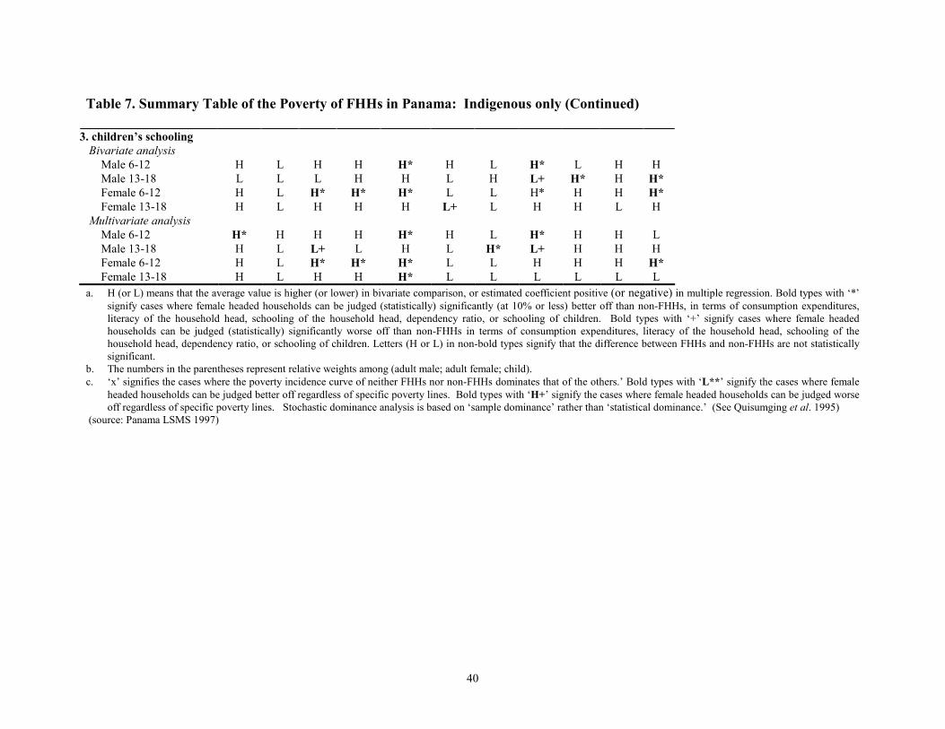
40

Table 7. Summary Table of the Poverty of FHHs in Panama: Indigenous only (Continued)


Bivariate analysis

Male 6-12 H L H H H* H L H* L H H

Male 13-18 L L L H H L H L+ H* H H*

Female 6-12 H L H* H* H* L L H* H H H*

Female 13-18 H L H H H L+ L H H L H


Male 6-12 H* H H H H* H L H* H H L

Male 13-18 H L L+ L H L H* L+ H H H

Female 6-12 H L H* H* H* L L H H H H*

Female 13-18 H L H H H* L L L L L L





significant.






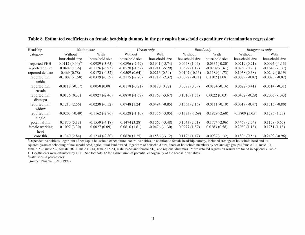
41

Table 8. Estimated coefficients on female headship dummy in the per capita household expenditure determination regressiona.

Headship Nationwide Urban only Rural only Indigenous only

category Without

household size

With

household size

Without

household size

With

household size

Without

household size

With

household size

Without

household size

With

household size

reported FHH 0.0112 (0.40) b. -0.0989 (-3.65) -0.0896 (-2.49) -0.1941 (-5.74) 0.0448 (1.04) -0.0335(-0.80) 0.0219 (0.21) -0.0095 (-1.13)

reported dejure 0.0407 (1.36) -0.1126 (-3.93) -0.0520 (-1.37) -0.1911 (-5.29) 0.0579 (1.17) -0.0709(-1.61) 0.0260 (0.20) -0.1648 (-1.37)

reported defacto 0.469 (0.78) -0.0172 (-0.32) 0.0509 (0.64) 0.0216 (0.34) -0.0107 (-0.13) -0.1189(-1.73) 0.1038 (0.68) -0.0249 (-0.19)

reported fhh:

unida

-0.1007 (-1.58) -0.0379 (-0.59) -0.2175 (-2.70) -0.1719 (-2.32) -0.0097 (-0.11) 0.1102 (1.08) -0.0089 (-0.07) -0.0023 (-0.02)

reported fhh:

casada

-0.0118 (-0.17) 0.0050 (0.08) -0.0178 (-0.21) 0.0170 (0.22) 0.0078 (0.09) -0.0134(-0.16) 0.0622 (0.41) -0.0514 (-0.31)

reported fhh:

div/sepa

0.0136 (0.33) -0.0927 (-2.46) -0.0870 (-1.68) -0.1767 (-3.67) 0.1010 (1.33) 0.0022 (0.03) -0.0432 (-0.29) -0.2005 (-1.43)

reported fhh:

widow

0.1213 (2.56) -0.0238 (-0.52) 0.0748 (1.24) -0.0494 (-0.85) 0.1363 (2.16) -0.0111(-0.19) -0.0017 (-0.47) -0.1715 (-0.80)

reported fhh:

single

-0.0203 (-0.49) -0.1162 (-2.96) -0.0528 (-1.10) -0.1356 (-3.05) -0.1373 (-1.69) -0.1829(-2.60) -0.5809 (5.05) 0.1795 (1.23)

potential fhh 0.1870 (5.13) -0.1559 (-4.18) 0.1474 (3.28) -0.1565 (-3.48) 0.1543 (2.51) -0.1774(-2.96) 0.4469 (2.74) 0.1158 (0.65)

female working

head

0.1097 (3.30) 0.0027 (0.09) 0.0616 (1.61) -0.0476 (-1.30) 0.0977 (1.89) 0.0283 (0.58) 0.2080 (1.18) 0.1751 (1.18)

core fhh 0.1340 (2.84) -0.1234 (-2.80) 0.0670 (1.25) -0.1586 (-3.12) 0.1196 (1.47) -0.0937(-1.32) 0.1806 (0.56) -0.2499 (-0.96) a.Dependent variable is: logarithm of per capita household expenditure; control variables, in addition to female headship dummy, included are: age of household head and its

squared, years of schooling of household head, agricultural land owned, logarithm of household size, share of household members by sex and age groups (female 0-4, male 0-4,

female 5-9, male 5-9, female 10-14, male 10-14, female 15-54, male 15-54 and female 54-), and regional dummies. More detailed regression results are found in Appendix Table

1. Coefficients were estimated by OLS. See footnote 32 for a discussion of potential endogeneity of the headship variables. b.t-statistics in parentheses.


42

Table 9. Estimated coefficients on female headship dummy in the school enrollment ratio regression (Female Children) a.


category Age 6-12 Age 13-18 Age 6-12 Age 13-18 Age 6-12 Age 13-18 Age 6-12 Age 13-18

reported FHH -0.0035(-0.60)

b.

-0.0461 (-1.57) -0.0163 (–1.49) -0.2261 (-2.76) c 0.0219 (0.96) -0.1120(-1.78) 0.0236 (0.33) 0.0058 (0.05)

reported dejure 0.0098 (0.85) -0.0460 (-1.23) 0.0002 (0.02) -0.2483 (-2.80) c 0.0274 (1.01) -0.1167(-1.63) -0.0973 (–0.88) -0.1802 (-1.42)

reported defacto -0.0216 (-0.47) -0.1315 (-1.41) -0.0627 (–0.99) -0.3094 (-2.66) -0.0226 (-0.28) -0.1177(-0.63) 0.2038 (2.94) 0.1866 (0.95)

reported fhh:

unida

-0.0144 (-0.44) -0.0062 (-0.11) -0.0691 (–1.36) -0.0599 (-0.70) -0.0134 (-0.33) -0.0092(-0.10) 0.1281 (2.36) 0.0056 (0.04)

reported fhh:

casada

0.0231 (1.93) d -0.0622 (-0.46) 0.0043 (0.57) -0.2331 (-1.03) 0.0552 (1.80) -0.1456(-0.60) 0.1971 (2.00) 0.4629 (1.99)

reported fhh:

div/sepa

0.0215 (1.90) -0.0375 (-0.78) 0.0131 (1.47) -0.4679 (-2.78) c 0.0474 (3.13) -0.0840(-0.85) -0.1525 (–1.09) -0.1207 (-0.72)

reported fhh:

widow

-0.0268 (-0.83) -0.0613 (-0.91) -0.0006 (–0.09) -0.0543 (-0.56) -0.0405 (-0.58) -0.0904(-0.83) -0.0382 (–0.19) -0.1653 (-1.17)

reported fhh:

single

0.0087 (0.44) -0.0018 (-0.04) -0.0143 (–0.95) -0.0073 (-0.15) 0.0524 (2.00) -0.0702(-0.60) 0.0560 (0.77) -0.2276 (-0.77)

potential fhh 0.0075 (0.40) 0.0365 (0.80) -0.0344 (–1.42) 0.0518 (0.99) 0.0505 (1.66) -0.0722(-0.80) 0.1102 (1.49) -0.0358 (-0.20)

female working

head

0.0102 (1.01) -0.0277 (-0.87) -0.0108 (–0.96) -0.2731 (-1.77) c 0.0373 (1.82) -0.1035(-1.56) 0.0631 (0.94) -0.1496 (-1.10)

core fhh 0.0063 (0.30) -0.0286 (-0.61) -0.0290 (–1.11) -0.5897 (-1.86) c 0.0598 (1.97) -0.1345(-1.32) 0.3631 (3.61) -0.2215 (-0.90)

a.Dependent variable is: the proportion of female children of age 6-12 or 13-18 who are enrolled in school to the total number of female children of the given age range; control

variables, in addition to female headship dummy, included are: age of household head and its squared, years of schooling of household head, logarithm of per capita household

expenditure agricultural land owned, logarithm of household size, share of household members by sex and age groups (female 0-4, male 0-4, female 5-9, male 5-9, female 10-14,

male 10-14, female 15-54, male 15-54 and female 54-), and regional dummies. More detailed regression results are found in Appendix Table 2. b.t-statistics in parentheses. c Coefficient was estimated by 2SLS when Hausman-Wu test rejects exogeneity of the headship variables. Identifying instruments for headship dummies were chosen among: a

dummy indicating the household member with highest education being male, a dummy indicating oldest household member being male and the amount of transfer income. All the

other coefficients were estimated by OLS. See footnote 34 for a discussion of potential endogeneity of the headship variables. d Bold letters signify that coefficient estimates are statistically significant at 10% level.


43

Table 10. Estimated coefficients on female headship dummy in the school enrollment ratio regression (Male Children)a.


category Age 6-12 Age 13-18 Age 6-12 Age 13-18 Age 6-12 Age 13-18 Age 6-12 Age 13-18

reported FHH 0.0361 (2.98) bd 0.1118 (0.38) -0.0596 (-1.80)

c -0.0032 (-0.10) 0.0577 (3.85) -0.0795(-1.34) 0.1536 (2.13) 0.0299 (0.26)

reported dejure 0.0287 (2.14) -0.0133 (-0.41) -0.0573 (-1.62) c -0.0137 (-0.38) 0.0516 (2.95) -0.1230(-1.83) 0.0911 (0.89) -0.0202 (-0.16)

reported defacto 0.0124 (0.42) 0.0278 (0.35) -0.0271 (–0.59) -0.0034 (-0.04) 0.0413 (2.28) -0.0039(-0.01) 0.1443 (1.27) -0.2396 (-2.22)

reported fhh:

unida

0.0393 (1.74) 0.0254 (0.40) -0.0060 (–0.18) -0.0636 (-0.82) 0.0599 (3.86) 0.0907 (0.67) 0.1081 (1.37) -0.0266 (-0.13)

reported fhh:

casada

0.0349 (3.07) 0.1272 (1.75) 0.0004 (0.02) 0.1473 (3.83) 0.0368 (1.94) -0.0648(-0.29) 0.2485 (2.64) 0.3741 (0.82)

reported fhh:

div/sepa

0.0081 (0.40) -0.0095 (-0.22) -0.0264 (–0.99) -0.0396 (-0.84) 0.0356 (1.62) 0.0009(0.01) 0.1484 (1.34) -0.0609 (-0.43)

reported fhh:

widow

0.1988 (1.03) 0.0177 (0.29) -0.6336 (-2.34) c 0.0457 (0.84) 0.0545 (2.24) -0.2878(-2.84) -0.2042(-0.72) 0.3157 (2.24)

reported fhh:

single

0.0352 (4.02) -0.0328 (-0.62) -0.0955 (-1.14) c -0.0106 (-0.18) 0.0306 (1.71) -0.1267(-1.33) 0.1665 (2.34) -0.3826 (-2.14)

potential fhh 0.0314 (1.66) -0.0358 (-0.61) 0.0039 (0.18) -0.0513 (-0.81) 0.0486 (1.50) -0.0599(-0.46) 0.0545 (0.45) 0.0870 (0.50)

female working

head

0.0115 (0.88) 0.0312 (0.97) -0.0048 (–0.33) -0.0199 (-0.55) 0.0192 (0.85) 0.1016 (1.37) 0.0487 (0.76) 0.0702 (0.43)

core fhh 0.0161 (0.83) -0.0220 (-0.38) -0.0115 (-0.45) -0.0028 (-0.05) 0.0557 (2.52) 0.0383 (0.26) -0.1500(-0.89) 0.0502 (0.29) a.Dependent variable is: the proportion of male children of age 6-12 or 13-18 who are enrolled in school to the total number of male children of the given age range; control

variables, in addition to female headship dummy, included are: age of household head and its squared, years of schooling of household head, logarithm of per capita household

expenditure agricultural land owned, logarithm of household size, share of household members by sex and age groups (female 0-4, male 0-4, female 5-9, male 5-9, female 10-14,

male 10-14, female 15-54, male 15-54 and female 54-), and regional dummies. More detailed regression results are found in Appendix Table 3. b. t-statistics in parentheses. c Coefficient was estimated by 2SLS when Hausman-Wu test rejects exogeneity of the headship variables. Identifying instruments for headship dummies were chosen among: a

dummy indicating the household member with highest education being male, a dummy indicating oldest household member being male and the amount of transfer income. All the

other coefficients were estimated by OLS. See footnote 34 for a discussion of potential endogeneity of the headship variables. d Bold letters signify that coefficient estimates are statistically significant at 10% level.


44

Appendix Table 1. Per-capita household expenditure determination regression (dep. var.: log of per capita household

expenditure) a.

Independent Nationwide Urban only Rural only Indigenous only

variables Without

household size

With

household size

Without

household size

With

household size

Without

household size

With

household size

Without

household size

With

household size

age -0.0071(-1.61) b 0.0216 (5.19) 0.0105 (1.95) 0.03826 (7.64) -0.0150 (-2.25) 0.0103 (1.63) -0.0322 (-1.43) -0.0075 (-0.39)

age squared 0.0079 (1.84) -0.0099 (-2.43) -0.0095 (-1.75) -0.0270 (-5.38) 0.0136 (2.17) -0.0014 (-0.23) 0.0291 (1.28) 0.0129 (0.66)

female headed 0.0112 (0.40) -0.0989 (-3.65) -0.0896 (-2.49) -0.1941 (-5.74) 0.0448 (1.04) -0.0335 (-0.80) 0.0219 (0.21) -0.1095 (-1.13)

household head

years of schooling

0.0988 (36.13)

0.0922 (36.75)

0.0753 (20.78)

0.0693 (20.26)

0.0934 (21.17)

0.0887 (21.64)

0.0508 (4.41)

0.0417 (3.84)

owned land 0.0001 (4.50) 0.0001 (5.87) 0.0009 (3.12) 0.0007 (2.07) 0.0017 (1.14) 0.0019 (1.36) 0.0001 (8.92) 0.0001 (10.27)

household size --- -0.6047(-22.10) --- -0.5778 (-16.46) --- -0.5703(-15.56) --- -0.5592 (-6.42)

share female 0-4 -1.8921(-14.37) -0.3840 (-2.80) -1.5272 (-8.69) -0.2207 (-1.20) -1.8470(-9.59) -0.3824 (-1.98) -1.8612( -3.08) -0.1759 (-0.29)

share female5-9 -1.5071(-12.68) -0.1680 (-1.37) -1.2691 (-7.57) -0.1205 (-0.72) -1.4274 (-8.55) -0.1137 (-0.65) -0.6703 (-1.06) 0.7918 (1.30)

share female 10-14 -1.2615(-10.91) -0.0127 (-0.10) -1.2059 (-7.50) -0.1822 (-1.10) -0.9726 (-5.87) 0.3222 (1.85) -0.4662 (-0.79) 0.8988 (1.48)

share female 15-54 -0.0366 (-.040) 0.7537 (8.04) -0.0837 (-0.64) 0.5528 (4.31) 0.2241 (1.83) 1.0136 (7.98) -0.6816 (-0.94) 0.4119 (0.64)

share female 55- 0.0903 (0.91) 0.3889 (4.10) 0.3071 (2.16) 0.5054 (3.74) 0.1355 (1.04) 0.3822 (3.07) -0.8610 (-1.09) -0.1038 (-0.15)

share male 0-4 -2.0893(-15.76) -0.5081 (-3.59) -1.4741 (-8.19) -0.1392 (-0.72) -2.1613(-12.11) -0.5801 (-3.08) -1.8860 (-2.93) -0.1064 (-0.17)

share male 5-9 -1.4990(-12.85) -0.1547 (-1.21) -1.2444 (-7.85) -0.0608 (-0.36) -1.4867 (-9.23) -0.2083 (-1.22) -1.0308 (-1.68) 0.4004 (0.66)

share male 10-14 -1.2566(-11.02) -0.0151 (-0.12) -0.9567 (-6.14) 0.0697 (0.45) -1.2591 (-8.19) 0.0219 (0.13) -0.5251 (-0.80) 0.8809 (1.32)

share male 15-54 -0.4302 (-5.49) 0.2923 (3.53) -0.4337 (-3.81) 0.1681 (1.43) -0.3213 (-3.10) 0.4006 (3.80) -0.2280 (-0.43) 0.6496 (1.31)

region 1 -0.5041(-16.56) -0.5086(-18.03) -0.3133 (-7.75) -0.3047 (-8.64) -0.0669 (-0.86) -0.0874 (-1.29) -0.1189 (-1.48) -0.1763 (-2.41)

region 2 -0.3330(-11.97) -0.3671(-14.15) -0.2076 (-6.39) -0.2160 (-7.46) -0.0621 (-0.80) -0.0917 (-1.35) ---c ---

c

region 3 -0.4177(-11.60) -0.4190(-12.74) -0.2046 (-4.58) -0.2244 (-5.51) -0.0153 (-0.19) -0.0282 (-0.40) ---c ---

c

Constant 7.3727 (52.20) 6.6075 (51.72) 7.1552 (40.69) 6.5254 (40.63) 7.1413 (33.10) 6.3809 (32.60) 5.0590 (9.00) 6.3074 (9.24)

adjust.R-squared 0.5833 0.6422 0.4450 0.5352 0.3955 0.4738 0.1581 0.2500

Sample size 4910 4910 2423 2423 2089 2089 398 398 a. Coefficient estimates on other control variables when female headship dummies with alternative definitions are used are very similar so are not displayed here but available upon

request. Coefficients were estimated by OLS. See footnote 32 for a discussion of potential endogeneity of the headship variables. b. t-statistics in parentheses. c. “indigenous areas,” as defined in the survey, do not exist in these areas.


45

Appendix Table 2. Determinants of school enrollment ratio of children (Female Children)

dependent variable: school enrollment ratio of girls age 6-12 or 13-18 a

Independent Nationwide Urban only Rural only Indigenous only

variables Age 6-12 Age 13-18 Age 6-12 Age 13-18 Age 6-12 Age 13-18 Age 6-12 Age 13-18

age 0.0039 (1.51)b 0.0096 (1.45) 0.0019 (0.87) 0.0086 (0.95) 0.0055 (1.51) 0.0187 (1.78) 0.0252 (1.39) 0.0204 (1.18)

age squared -0.0035(-1.42) -0.0106 (-1.57) -0.0018 (-0.99) -0.0071 (-0.82) -0.0047 (-1.31) -0.0211 (-2.01) -0.0243(-1.35) -0.0184 (-1.02)

female headed 0.0070 (0.60) -0.0461 (-1.39) -0.0163 (-1.48) -0.0631 (-1.39) 0.0219 (0.96) -0.1120 (-1.78) 0.0236 (0.33) 0.0058 (0.05)

household head

years of schooling

0.0013 (0.95)

0.0069 (6.41)

-0.0009(-0.78)

0.0060 (1.48)

0.0050 (1.57)

0.0058 (0.81)

0.0100 (1.43)

0.0244 (1.90)

owned land -0.0001(-43.5) -0.0001 (-7.76) ---c 0.0092 (2.57) 0.0004 (0.80) 0.0006 (2.46) -0.0001(-9.15) -0.0001 (-3.89)

Log per-capita

household

expenditure

0.0407 (4.01)

0.1558 (6.41)

0.0103 (1.24)

0.0512 (1.25)

0.0353 (2.36)

0.2252 (6.11)

0.0824 (1.86)

0.1309 (2.47)

log(household size) -0.0060(-0.37) 0.0780 (1.56) -0.0325(-1.74) 0.0076 (0.10) 0.0325 (1.39) 0.1145 (2.09) -0.0360(-0.51) 0.0654 (0.60)

share female 0-4 0.0133 (0.13) -0.5642 (-1.68) 0.1133 (1.34) -0.4649 (-0.93) -0.0454(-0.26) -0.4286 (-0.90) -0.5354 (-0.85) 0.6159 (0.52)

share female5-9 -0.0389(-0.44) -0.1016 (-0.36) -.0432(-1.00) 0.1777 (0.50) 0.0768(0.47) -0.3347 (-0.77) -0.7548 (-1.35) 1.1764 (1.00)

share female 10-14 -0.0318(-0.37) 0.7418 (2.75) -0.0549(-1.05) 0.7747 (2.33) 0.0831 (0.51) 0.6437 (1.51) -.04846(-0.87) 2.1464 (1.76)

share female 15-54 -0.0297(-0.32) 0.1366 (0.53) 0.0729 (1.00) 0.2946 (0.92) -0.0992(-0.60) -0.0693 (-0.17) -0.5546(-0.90) 1.7468 (1.42)

share female 55- -0.0856(-0.75) 0.3307 (1.13) 0.1208 (1.47) 0.3731 (1.06) -0.2344(-1.00) 0.3931 (0.78) -0.9158(-1.11) 1.7707 (1.70)

share male 0-4 -0.0967(-0.92) -0.4941 (-1.55) 0.0080 (0.10) -0.5736 (-1.25) -0.1602(-1.02) -0.4815(-1.07) -0.7095(-1.10) 1.6056 (1.41)

share male 5-9 0.0305 (0.29) 0.2941 (1.01) 0.0316 (0.31) 0.5167 (1.36) 0.0296 (0.17) 0.0848 (0.20) -0.3730(-0.67) 1.4133 (1.22)

share male 10-14 -0.0258(-0.24) 0.0079 (0.03) 0.0265 (0.27) 0.1986 (0.58) -0.0597(-0.34) -0.2025(-0.48) -0.7430(-1.18) 0.9591 (0.84)

share male 15-54 -0.0238(-0.32) -0.1604 (-0.65) 0.0353 (0.73) 0.0772 (0.24) -0.0378(-0.30) -0.5154 (-1.43) -0.7209(-1.31) 0.6461 (0.57)

region 1 0.0029 (0.24) 0.0612 (1.90) 0.0056 (0.44) 0.1365 (3.82) 0.0272 (0.52) -0.1943 (-2.33) -0.0496 (-1.19) -0.0152 (-0.19)

region 2 0.0002 (0.02) 0.0816 (2.58) 0.0040 (0.30) 0.0636 (1.72) -0.0041 (-0.08) -0.1534 (-1.98) ---d ---

d

region 3 0.0204 (1.96) 0.0449 (1.17) 0.01787 (2.45) 0.0960 (1.71) 0.0257 (0.49) -0.1802 (-2.07) ---d ---

d

constant 0.6047 (4.61) -0.8701 (-3.00) 0.9049 (8.59) -0.1305 (-0.32) 0.5038 (2.26) -1.1854 (-2.39) 0.4314 (0.66) -2.3972 (-2.01)

adjust.R-squared 0.078 0.2562 0.0492 0.1893 0.0517 0.2321 0.1574 0.2274

Sample size 1285 1082 543 510 538 423 204 149 a Coefficient estimates on other control variables when female headship dummies with alternative definitions are used are very similar so are not displayed here but available upon

request. Coefficients were estimated by OLS. See footnote 34 for a discussion of potential endogeneity of the headship variables. b t-statistics in parentheses. c Land variable dropped due to the small variation in the sample. d “indigenous areas,” as defined in the survey, do not exist in these areas.


46

Appendix Table 3. Determinants of school enrollment ratio of children (Male children)

dependent variable: school enrollment ratio of boys age 6-12 or 13-18a Independent Nationwide Urban only Rural only Indigenous only

variables Age 6-12 Age 13-18 Age 6-12 Age 13-18 Age 6-12 Age 13-18 Age 6-12 Age 13-18

Age 0.0005 (0.16) b 0.0115 (1.82) 0.0020 (0.62) 0.0277 (2.91) 0.0013 (0.27) 0.0072 (0.71) 0.0077 (0.51) -0.0018 (-0.10)

age squared -0.00004(-0.02) -0.0073 (-1.17) 0.0001(0.15) -0.0215(-2.17) -0.0006 (-0.14) -0.0038 (-0.41) -0.0145 (-0.91) 0.0015 (0.08)

female headed 0.0361 (2.98) 0.0112 (0.38) -0.0097(-0.49) -0.0033(-0.10) 0.0577 (3.85) 0.2395 (1.34) 0.1536 (2.13) 0.0299 (0.26)

Household head

years of schooling

0.0029 (2.09)

0.0175 (5.95)

0.0027 (1.72)

0.0072 (2.09)

0.0021 (0.68)

0.0277 (4.49)

0.0117 (1.90)

0.0307 (2.57)

owned land 0.00001 (3.53) -0.0001 (-11.07) 0.00003(0.20) -0.0032 (-0.43) 0.00004 (0.07) -0.0030 (-2.26) 0.00001 (1.14) -0.0001 (-4.01)

Log per-capita

household

expenditure

0.0355 (2.38)

0.2082 (10.68)

-0.0221(-0.68)

0.1333 (4.65)

0.0321 (1.95)

0.2395 (6.92)

0.1178 (3.08)

0.1480 (2.52)

log(household size) -0.0330 (-0.97) 0.0643 (1.69) -0.0957(-1.61) 0.0139 (0.30) -0.0229 (-0.67) -0.0551(0.77) 0.0870 (1.13) 0.0902 (0.79)

share female 0-4 0.0659 (0.31) -0.1329 (-0.49) 0.3254 (0.89) 0.0529 (0.14) 0.0894 (0.53) -0.2152 (-0.48) -1.3179 (-1.78) -0.9883 (-1.02)

share female5-9 0.0870 (0.52) 0.2696 (1.20) 0.3102 (1.15) 0.4352 (1.51) 0.0696 (0.42) 0.3283 (0.90) -1.3577 (-1.88) -0.7031 (-0.74)

share female 10-14 0.0700 (0.35) 0.2943 (1.41) 0.2794 (0.84) 0.5902 (2.29) 0.0247 (0.14) 0.2182 (0.64) -1.0996 (-1.88) -1.3088 (-1.43)

share female 15-54 -0.0240 (-0.14) 0.2338 (1.22) 0.1870(0.64) 0.3857 (1.61) 0.0997 (0.63) 0.0759 (0.23) -1.4118 (-2.08) -0.9210 (-1.06)

share female 55- -0.0324 (-0.23) 0.0959 (0.41) 0.1726 (0.80) 0.3427 (1.27) -0.0708 (-0.44) -0.0069 (-0.02) -1.5004 (-1.46) -0.6317 (-0.61)

share male 0-4 0.1520 (0.75) 0.6022 (2.51) 0.3215 (0.89) 0.6228 (1.97) 0.1774 (1.08) 0.7548 (1.85) -1.0015 (-1.52) -0.6143(-0.70)

share male 5-9 -0.0161 (-0.08) 0.2928 (1.25) 0.2360(0.69) 0.4205 (1.32) -0.0415 (-0.27) 0.2098 (0.56) -1.4175 (-2.16) -1.1348 (-1.22)

share male 10-14 0.0184 (0.10) 0.6401 (3.46) 0.2245(0.71) 0.8079 (3.44) 0.0312 (0.17) 0.5723 (1.94) -1.2236 (-1.71) -0.4830 (-0.50)

share male 15-54 0.0737 (0.40) 0.0181 (0.10) 0.2687 (0.85) 0.2639 (1.14) 0.0661 (0.54) -0.1612 (-0.58) -1.2172 (-1.85) -1.5003 (-1.84)

region 1 0.0158 (1.23) 0.0889 (2.78) 0.0295 (2.12) 0.1276 (3.45) -0.0365 (-2.40) 0.1967 (1.68) -0.0449 (1.01) 0.1431 (1.63)

region 2 0.0214 (1.54) 0.0299 (0.93) 0.0166 (1.00) 0.1087 (2.85) -0.0529 (-3.09) 0.1390 (119) ---c ---c

region 3 0.0215 (1.41) 0.0198 (0.53) 0.0376 (2.80) 0.1320 (3.40) -0.0558 (-2.67) 0.0975 (0.80) ---c ---c

constant 0.6764 (4.73) -1.6049 (-6.20) 0.9309 (6.10) -1.4659 (-4.12) 0.7114 (2.84) -1.7672 (-3.90) 1.2180 (1.52) 0.4498 (0.48)

adjust.R-squared 0.0511 0.2895 0.0519 0.2182 0.0038 0.2331 0.1388 0.2312

Sample size 1351 1168 559 510 572 492 220 166 aCoefficient estimates on other control variables when female headship dummies with alternative definitions are used are very similar so are not displayed here but available upon

request. Coefficients were estimated by OLS. See footnote 34 for a discussion of potential endogeneity of the headship variables. b t-statistics in parentheses. c “indigenous areas,” as defined in the survey, do not exist in these areas.


Documents

World Development abstract - 千葉大学園芸学部 · Gonzalez, all of the Ministry of Planning and Economic Policy (MIPPE) of Panama, and two anonymous referees as well as the