Working paper nr

SVERIGES RIKSBANK WORKING PAPER SERIES 347

On the effectiveness of loan-to-value regulation in a multiconstraint framework

Anna Grodecka

November 2017

WORKING PAPERS ARE OBTAINABLE FROM

www.riksbank.se/en/research Sveriges Riksbank • SE-103 37 Stockholm

Fax international: +46 8 21 05 31 Telephone international: +46 8 787 00 00

The Working Paper series presents reports on matters in the sphere of activities of the Riksbank that are considered

to be of interest to a wider public. The papers are to be regarded as reports on ongoing studies

and the authors will be pleased to receive comments.

The opinions expressed in this article are the sole responsibility of the author(s) and should not be interpreted as reflecting the views of Sveriges Riksbank.

http://www.riksbank.se/en/research

On the effectiveness of loan-to-valueregulation in a multiconstraint framework

Anna Grodecka∗

Sveriges Riksbank Working Paper Series

No. 347

November 2017

Abstract

Models in the infinite horizon macro-housing literature often assume that borrowers are con-strained exclusively by the loan-to-value (LTV) ratio. Motivated by the Swedish micro-data,I explore an alternative arrangement where borrowers are constrained by the feasibility of re-payment, but choose a house of maximum permissible size conditional on the LTV restriction.While stricter LTV limits are often considered as a measure to tackle the rise in householdindebtedness, I find that policy designed to lower the maximum permissible LTV ratio mayactually leave the debt-to-GDP ratio unchanged and increase housing prices in equilibrium ifborrowers are bound by two constraints at the same time. In a model with occasionally bind-ing constraints, I show that also for the analysis of the short-run effects of different policies,the consideration of multiple constraints, possibly binding at the same time, is important. Theeffectiveness of LTV as a measure to tackle the rise in indebtedness has to be reassessed and islikely lower than previously shown.

Keywords: borrowing constraints, household indebtedness, macroprudential policy, housingprices, loan-to-value ratio, debt-service-to-income ratioJEL-Classification: E32, E44, E58, R21

∗ Sveriges Riksbank, e-mail: [email protected]. I would like to thank Daria Finocchiaro, Paolo Gior-dani, Isaiah Hull, Peter van Santen and Karl Walentin for comments, as well as the participants in the Riks-bank Research Seminar, Finansinspektionen, Verein fuer Sozialpolitik 2017 conference, the EcoMod 2017 andGreater Stockholm Macro Group meeting. The views expressed in this paper are solely the responsibility of theauthor and should not be interpreted as reflecting the views of Sveriges Riksbank.

1

Anna Grodecka: On the effectiveness of loan-to-value regulation in a multiconstraint framework

1. Introduction

Which macroprudential measures are most effective in addressing household indebtedness?Empirical studies studying this question face the challenge of the coexistence and comovementof multiple measures in the same country at the same time, which makes measuring the effectof one single policy difficult. This identification difficulty makes a strong case for studyingthe impact of these measures in a structural model in which different channels can be shutdown, and thus, separated. Among popular macroprudential tools, many theoretical papersadvocate the use of stricter loan-to-value (LTV) policy as a very effective measure reducinghousehold indebtedness, which lowers house prices as well (see Chen and Columba, 2016 andFinocchiaro, Jonsson, Nilsson, and Strid, 2016 for Sweden, Alpanda, Cateau, and Meh, 2014for Canada), but they do mostly so in the models where the LTV constraint is the only constraintimposed on borrowers, following Iacoviello (2005). This may overstate the effectiveness ofLTV limits in affecting the debt in real economies, where multiple constraints are applied toborrowers and may interact.

In this paper, using a simple real business cycle model with short-term debt, and its New-Keynesian extension with long-term debt, I argue that in a framework where both LTV limitsand debt repayment limits (debt service to income ratio - DSTI) are imposed on borrowers,tighter LTV regulation may have no effect on household indebtedness ratios (defined as debt toGDP or debt to income) and may actually lead to an increase in housing prices in equilibrium.This happens if borrowers are both at their LTV limit and at the DSTI limit at the same time.Bindingness of two borrowing constraints imposes a direct relation between borrowers’ laborincome and the value of their housing stock implying a constant debt to GDP ratio for differentLTV ratios, equal to the DSTI limit. Thus, changing LTV will not affect debt to GDP ratios,while changing DSTI will. Under a realistic distribution of borrowers across different con-straints, in equilibrium, the effectiveness of LTV in influencing debt-to-GDP ratios is greatlyreduced. Apart from analyzing long-run implications of different macroprudential policies,in order to study business cycle implications of two possibly binding constraints, I considera model with occasionally binding constraints with four regimes allowing for different com-binations of slack and binding constraints. Even if one of the constraints is slack in a givenperiod, its presence and potential future bindingness affects the behaviour of indebted house-holds. Hence, the interaction of the LTV and DSTI constraints is important for the dynamicsof indebtedness ratio and housing prices in the economy.

While the effect of LTV regulation has been extensively studied in the literature, the interac-tion between the LTV constraint and the DSTI constraint has not gained much attention so far,apart from a recent study of Greenwald (2016).1 However, their coexistence is fairly common

1 Admittedly, the heterogeneous agents literature studying household borrowing in an overlapping generations

2


both in advanced and emerging economies and increasingly many countries are consideringimplementing DSTI measures along with existing LTV measures, given that it has been foundthat sound debt repayment ratios contribute to financial stability and reduce banks’ portfoliorisk (see Dietsch and Welter-Nicol, 2014). In some countries, like Canada or Estonia, regula-tion explicitly sets the upper limit on the LTV and DSTI ratios, in other, like Sweden or France,it is the banking practice to look at both components while deciding on the loan application.

If many borrowers in a given economy in addition to the LTV constraint are bound also bythe DSTI constraint, lowering LTV is a very ineffective policy, if the aim is to reduce debt toincome or debt to GDP. In the extreme scenario in which all borrowers are both at their LTVand at their DSTI limits, stricter LTV policy not only does not influence debt ratios at all, butit also drives house prices up in the equilibrium. Ceteris paribus, if the debt level is determinedby a DSTI limit and one unit of housing can pledge less collateral, its value has to increaseif it has to collateralize the same amount of debt. A similar mechanism is described in anexample in a recent paper by Greenwald (2016). It presents a model for the U.S. in whichnew borrowing is determined by an LTV and a payment to income constraint. Borrowersswitch between being bound by each of constraints and in equilibrium, only one constraint isbinding for a given type of borrower. This is different from the setup presented in this paper.First, I consider a model with DSTI and LTV constraints and show that in equilibrium bothof them can bind at the same time. Second, I simulate an economy with occasionally bindingconstraints. As a result of shocks hitting the economy, either one or both considered constraintsmay become slack and the dynamic model simulations take into account the existence of fourpossible regimes in which: both constraints bind, only the DSTI constraint binds, only theLTV constraint binds, or neither the DSTI, nor the LTV constraint bind. As Guerrieri andIacoviello (2017) show, taking into account the occasionally binding constraints has crucialimplications for considering possible asymmetries arising during the business cycles. However,while Guerrieri and Iacoviello (2017) show it for an LTV-only model in the presence of verylarge housing preference shocks, I demonstrate that in the model with multiple occasionallybinding constraints, sizable asymmetries arise even in the presence of relatively small shocks.

The mechanism described in this paper is crucial for the analysis of macroprudential policiesin countries with multiple constraints. It may be relevant even for countries without an estab-lished DSTI limit, if borrowers, aside of the banks, impose such a limit on themselves. Thereis evidence for the euro area and U.S. that the debt service to income ratios are approximatelystable in the long run (see European Central Bank, 2005; BIS, 2017; Federal Reserve Board,2017). Obviously, the extent to which the mechanism presented in this paper will be relevant

setup (see e.g. Iacoviello and Pavan, 2013 and Hull, 2015) takes into account the coexistence of two constraints.However, the interaction of constraints is not explicitly studied in these papers. In the infinite horizon setup,Gelain, Lansing, and Mendicino (2013) consider an example with a combined borrowing constraint, wheredifferent weights are attached to the LTV and to the loan-to-income assessment.

3


for a given country can be only assessed using the micro-data with detailed information onthe constraints faced by individuals. Having access to the Swedish data, I am able to makesuch an assessment for Sweden, showing that the share of constrained borrowers that are con-strained both by LTV and DSTI constraint is non-negligible. These are predominantly younghouseholds, most likely to be relatively more constrained than an average borrower due to ashort saving history and hence, potentially low downpayment, and a relatively lower wage in-come. First-time borrowers often maximize their loan amount as given by the DSTI limit, andscrounge money from parents and relatives for the minimum downpayment. Moreover, in thebroader perspective, the dynamic implications of multiple possibly binding constraints becomeimportant in events of severe crises, when both house prices go down and the income of thehouseholds suffers due to an increased unemployment rate. The Swedish 1990s banking crisisis an example of such an environment, as is the recent Great Recession in the U.S.

While my paper mostly refers to the theoretical macroeconomic literature in the infinitehorizon setup that has predominantly neglected the existence of DSTI constraint so far, it isimportant to note the existence of empirical studies that focus on establishing links betweendifferent macroprudential measures and changes in them and credit. Some of them focus onDTI and LTV limits (see Cerutti, Claessens, and Laeven, 2017 and Crowe, Dell’Ariccia, Igan,and Rabanal, 2013) and show that there is a mixed empirical evidence of longer run effec-tiveness of macroprudential measures, less than the one suggested by theoretical contributions,which may be due to interaction between particular constraints that was mostly absent in thetheoretical frameworks so far. DSTI limits seem to be more prevalent than DTI ratios. Akinciand Olmstead-Rumsey (2017) perform panel regressions for 57 countries in years 2000-2013to assess the effectiveness of different measures (including DSTI) in affecting credit growthand house price appreciation. They note that the LTV and DSTI caps are often used simultane-ously, which may be a problem for identification of their separate effects in empirical work andmakes a strong case for studying the impact of these measures in a structural model in whichdifferent channels can be shut down, and thus, separated. Akinci and Olmstead-Rumsey (2017)conclude that DSTI caps have a stronger effect on housing credit than the LTV caps, whichsupports my theoretical results.

In the following, in section 2, I present some empirical evidence with emphasis on Sweden,followed by the exposition of the basic idea of the paper in a simple real business cycle modelwith one-period debt in section 3. I compare the long-run and short-run implications of themodel with two constraints to a model with LTV and DSTI constraint only. In order to be ableto compare a broader range of macroprudential instruments in a realistic setup, in section 4, Iextend the simple model with one-period debt to a New-Keynesian setup with long-term debt,where I show the equilibrium effects of changes in the LTV ratio, amortization rate, and DSTIratio, as well as dynamic responses of economies to different shocks, comparing the multiple

4


Country LTV-limit DSTI-limitCanada 95% 39-44%a

China 70% 50%Cyprus 80% 35%Estonia 85% 50%

Hong Kong 70% 50%Hungary 80%b 10-60%

Israel 75% 50%Korea 50-70% 50-60%

Lithuania 85% 40%Netherlands 100% 10-38%c

Singapore 80% 60%Slovenia 80% 50%

Notes: The table has been created using the information from Eesti Pank (2014), European Systemic RiskBoard (2015), Bank of Slovenia (2016), European Systemic Risk Board (2017), International MonetaryFund, 2017.

a The limit for the gross and total debt service respectively.b This is the limit for loans in HUF, for other currencies it is lower.c The DSTI limit depends on the income.

Table 1: The contemporaneous usage of explixit LTV and DSTI limits in different countries

constraint model with a DSTI-only and LTV-only model.

2. Empirical evidence

The mechanism presented in this paper may be observed in countries, in which multiplesimultaneously binding constraints are applied to loan applicants. In this paper, I focus onLTV and DSTI measures whose usage is highly correlated both in advanced and in emergingeconomies (Akinci and Olmstead-Rumsey, 2017).2 Table 1 presents the regulatory limits set inadvanced and emerging economies that implement both of these constraints at the same time.

Countries presented in Table 1 set explicit limits on the discussed ratios. In other countries,it is the banking practice to look at both components while deciding on the loan application:in Brasil, Colombia, Malaysia and Thailand banks tend to put more weight on the assessmentof borrowers’ financial capacity to settle loan installments rather than their LTV (de Carvalho,Castro, and Costa, 2014 and He, Nier, and Kang, 2016), in France, along with a downpaymentrequirement, banks use a so-called 33% rule under which the debt burden should not exceed

2 Note that the DTI limit, present in some countries along with a LTV regulation, is very similar in spirit to aDSTI limit. However, the DSTI limit changes with changes in interest rates, while DTI not. In this paper, Ifocus on the DSTI limit.

5


one third of households’ income (Dietsch and Welter-Nicol, 2014). Greenwald (2016) reportsregulatory payment to income and LTV limits for the U.S. In some countries, banks lendingpractices follow the regulatory guidelines, that are, however, not formal requirements. Thisis the case of Sweden, where banks perform a discretionary income calculation along withthe assessment of the downpayment. Such an assessment is also performed in Latvia, Poland,Romania, Slovakia and in the Czech Republic (see Fell, 2015, European Systemic Risk Board,2016, European Systemic Risk Board, 2017).

2.1. The mortgage process in Sweden

In Sweden, the Swedish Financial Supervisory Authority (Finansinspektionen) issues gen-eral guidelines to banks regarding the mortgage lending. Since 1st October 2010, a guidelineregarding the maximum LTV applies: “When a firm grants a loan collateralised by a home

the loan should be limited such that the loan-to-value ratio for the home does not exceed 85

per cent of the home’s market value at the time the loan is granted. This limitation to the

loan-to-value ratio should be established in the firm’s credit instructions, where applicable.”

(Finansinspektionen, 2010b). In 2004, a guideline about a DSTI-type of assessment for creditinstitutions and investment firms has been issued: “The credit assessment should be based on

information that provides an accurate picture of the credit applicant’s financial status. It should

include a sensitivity analysis of the credit applicant’s repayment capacity and an assessment of

the risk for a deterioration in the value of collateral.” (Finansinspektionen, 2004). Followingthis guidline, in the banking practice, the Swedish DSTI constraint takes the form of a ’discre-tionary income’ limit (see Finansinspektionen, 2010a, Sveriges Riksbank, 2014 and Li and vanSanten, 2017). Banks use the so-called KALP ("kvar att leva på" - the amount left to live on,also called discretionary income) calculation to establish the borrowing limit of a household.This calculation takes into account borrowers after-tax income, transfers, minimum consump-tion, housing expenses (including amortization and loan payments) and a stressed-interest rateto ensure that the borrower can cope with the loan installments even in an event of an interestrate hike. Despite being slightly different, in modeling terms, it has similar implications forhouseholds’ borrowing limit as the DSTI constraint (see Appendix A) and thus, in the modelpart I choose to work with the DSTI constraint for the sake of model universality.

In the Swedish housing market, housing transactions are a result of a bidding process, inwhich the highest bidder usually acquires the apartment. Before participating in the biddingprocess, future borrowers obtain from a bank a promise of loan (so-called lånelöfte) statingtheir borrowing limit. Given household’s income, house prices and a minimum downpayment,the KALP constraint determines the borrowing amount and the LTV constraint the value of thehouse that can be purchased by the borrower (in reality, more choices regarding housing can

6


be made that in the model: size, location, new- vs old-construction etc.). If the discretionaryincome calculation sets a limit of the loan to B and the LTV requirement is 85%, the maximumvalue of the house that that customer can acquire (without taking unsecured debt) isB/LTV =

1.18B. Given that information and prevailing house prices in different areas, the agent makesthe housing decision.3

Naturally, the guidelines help the banks in establishing the upper loan limit and if the loanapplicant decides to borrow less than the limit, it is possible that neither of the constraints binds.The extent of bindingness of constraints is an empirical question and I address it by looking atthe micro-evidence for Sweden.

2.2. Descriptive evidence from the Swedish micro-data

To establish the economic importance of the mechanism described above, I refer to themicro-data from the Swedish mortgage survey conducted every year by Finansinspektionen,the Swedish Financial Supervisory Authority. The data used covers all new mortgage loansgiven out by 8 largest banks in Sweden in years 2011-2015 in a few weeks between Augustand October.4 The delivered data contains detailed borrowers and loan characteristics.5 The

3 In a static setup with fixed income, the LTV limit determines the housing choice and not the borrowing amountas in a traditional Iacoviello (2005) setup. In the dynamic setup, both housing and labor decisions will beadjusted contemporaneously to account for the existence of both constraints. In this situation, tighter LTVregulation leads to an absolute decrease in household borrowing. However, the debt to GDP ratio does not godown, as wage income, debt and output comove.

4 Note that the 2016 data is also available, but following Finansinspektionen’s request, banks changed in this yeartheir definition of the discretionary income, so that the actual discretionary income used by the banks whilegranting the loan is not available for 2016. Under certain assumptions, a proxy of banks’ discretionary incomecalculation can be computed and the distribution of borrowers is very similar to years 2011-2015, not changingthe fractions used for the calibration of the theoretical model. However, given the coherent variable definitionsin years 2011-2015, I choose to restrict my analysis in this paper to these years. Note that before June 2016, noamortization requirement was formally present in Sweden. Since June 2016, a minimum amortization require-ment is applied to new mortgages with an LTV above 50%: 1 percent annually for mortgages with LTV between50 and 70%, and 2 percent annually for mortgages with an LTV above 70% (see Finansinspektionen, 2016).This directly affects the KALP calculations of the banks and could change the distribution of new borrowersacross constraints considerably. However, since after the introduction of the amortization requirement, bankslowered other costs included in their discretionary income calculation to offset the strenghtened amortizationrules (which can be thought of as a simultaneous reduction in the DSTI limit), in practice, the distributions ofborrowers across the constraints did not change much.

5 Given the survey nature of the dataset, it covers only a subset of new mortgage loans in Sweden every year.However, I compare the aggregate statistics in the survey with the implied characteristics from the UC creditdataset covering all borrowers in Sweden on a monthly basis from 2011 to 2016. Despite the larger size, theUC credit dataset is not suitable for the analysis presented in this paper, as it does not contain house valuesfor borrowers living in apartments (thus, only house owners can be taken into account when considering theLTV ratio and even then, the housing values in the dataset are not corresponding to market values), neitherdoes it contain detailed information on the loan characteristics, such as the type and level of the interest rate,monthly amortization etc. Thus, after making sure that the mortgage survey statistics is representative for thepopulation of new borrowers in Sweden by comparison of borrowers’ characteristics in both datasets, I continuethe analysis with the mortgage survey data.

7


010

2030

40P

erce

nt

0 .2 .4 .6 .8 1.85LTV

All borrowers Borrowers under 35 years old

(a) The distribution of LTV 2011-2015

05

1015

20P

erce

nt

-50000 0 50000

3000

Monthly Surplus Amt

All borrowers Borrowers under 35 years old

(b) The distribution of KALP 2011-2015

Figure 1: Distributions of constraints for new borrowers in Sweden, 2011-2015

mortgage survey data, apart from detailed mortgage characteristics, contains bank’s evaluationof the bindingness of the borrower’s KALP constraint. If the KALP value in the dataset is 0 (orin exceptional cases, below 0), it indicates that the household maximized its borrowing limit.

Figure 1 presents the distribution of values for LTV and KALP among the borrowers for years2011-2015, with the whole population indicated with blue bars, and the young population, de-fined as under 35 years, indicated by transparent bars with black borderline. The bunching ofborrowers around the limits suggested by regulatory guidelines indicates that banks follow theguidelines even though they are not established as strict regulation. The left panel presentsthe histogram for LTV ratios (both collateralized debt and uncollateralized debt to finance themortgage is taken into account in the LTV calculation, hence values of over 85% are possible),with a visible spike around 85%, the regulatory guideline for new mortgages in Sweden. Thespike is more accentuated for borrowers under 35 years old who are more likely to be trulyfirst borrowers (unfortunately, the dataset may contain people who switch banks but are notfirst-time mortgage borrowers). They can be more affected by constraints due to a shorter workand thus, savings, history. The right panel of Figure 1 presents the distribution of KALP valuesamong the surveyed population of borrowers. Some first time mortgage borrowers have theKALP below 0, which indicates that they borrowed up to the maximum amount and beyond.Moreover, we see that the distribution of KALP values is skewed towards zero, with a spikeclose to 0, indicating that many more borrowers are approximately constrained by the discre-tionary income calculation of the bank. Similarly to the LTV distribution, we note that for theborrowers under 35 years old the distribution is skewed towards the maximum specified in Fi-nansinspektionen’s guidelines. The shape of the histograms and their spikes around regulatorylimits indicate that both constraints are important for the borrowers (and banks).

Figure 1 shows the whole distribution of new borrowers in Sweden across different con-

8


straints, which does not mean that they are all actually credit constrained. Given the regulatoryguidelines, only borrowers that are reasonably close to the suggested thresholds should be con-sidered credit constrained. For the purpose of this paper, I define a KALP-constrained agentas an individual whose KALP-value in the database is below 3000 SEK (around 300 EUR, itmeans that a given person has 300 EUR monthly left after the repayment of all debt obligations,housing expenses and minimum consumption expenses in the stressed interest rate scenario).Similarly, given a regulatory LTV limit of 85%, I define as LTV-constrained agents individualswith an LTV larger than 80%. To test for the importance of a (non-existing) debt to income(DTI) constraint, I define DTI-constrained agents as individuals with a DTI larger than 6. Theresults of this exercise are presented in Figure 2. On average, in years 2011-2015, 33 percent

0,00

0,10

0,20

0,30

0,40

2011 2012 2013 2014 2015Percen

tage of all bo

rrow

ers

Fraction of borrowers constrained by different constraints

DTI above 6 LTV above 0.8 KALP below 3000 SEK

Figure 2: Fraction of borrowers constrained by different constraints in the Swedish mortgagesurvey data, 2011-2015

of new borrowers were constrained by the LTV constraint, 19 percent of new borrowers wereKALP-constrained, and only 2 percent of new borrowers can be defined as DTI-constrained. Iconsider the remaining borrowers as non-constrained. Given the nonexistence of a DTI con-straint in Sweden and a small number of new borrowers that could be potentially constrained bysuch a regulation, in the following, I focus on the LTV- and KALP-constrained borrowers and Idefine a subset of new borrowers consisting of people having an LTV higher than 80% and theKALP value below 3000 SEK. Figure 3 presents the distribution of these constrained borrow-ers among the main types of constraints (aggregate for years 2011-2015). We can see that theshare of borrowers constrained by both the LTV- and the KALP-constraint is non-negligible,

9


as it accounts for 14%. Moreover, in the subset of constrained borrowers, ”merely” 60% ofhouseholds are constrained only by the LTV-constraint - ”merely” with respect to the modelsused for analysis of the effectiveness of LTV regulation for Sweden, which assume that thisshare is 100% (see Chen and Columba, 2016 and Finocchiaro et al., 2016). It might seem thatthe occurrence of agents constrained by both constraints is a relatively unlikely phenomenon,but if we think of a young borrower with little savings and low income, the 14% figure is notsurprising. First-time borrowers often maximize their loan amount as given by the DSTI limit,and scrounge money from parents and relatives for the minimum downpayment. In the follow-ing, in Section 3, I formulate a simple model with one-period debt to illustrate the idea behindthe two borrowing constraints binding at the same time and explain the intuition looking at thelong-run and short-run implications of LTV regulation is such a setup, compared to a modelwith LTV constraint only or DSTI constraint only. In section 4, I extend this setup to considerlong-term debt and in a model matching the Swedish data, I study the equilibrium effects ofchanges in macroprudential policies given the distribution of borrowers across constraints aspresented in Figure 3.

OnlyLTV‐constrained

60%

OnlyKALP‐constrained

26%

LTV‐ and KALP‐constrained

14%

Figure 3: The distribution of constrained borrowers in Sweden among the LTV and the KALP-constraint

3. Simple Model with One-Period Debt

I start the exposition of the main idea from a real business cycle economy, where all debtcontracts take the form of one-period debt. Consider an economy populated by firms andhouseholds that differ in their degree of impatience. Firms operate in a competitive marketand are profit maximizers. They use labor to produce the final good. Households derive utilityfrom leisure, consumption and housing. Patient households (’savers’) provide one-period loansto impatient households (’borrowers’). Only borrowers are subject to credit constraints. They

10


are subject to LTV and DSTI constraints. In the following, I present the borrower’s problem(savers’ and firms’ first-order-conditions (FOCs) are standard and presented in Appendix B).

3.1. Impatient households

Impatient households get utility from goods and housing consumption, as well as leisure.They provide labor to firms and borrow from savers subject to two borrowing constraints.

Impatient households have the following utility function:

maxbBt ,h

Bt ,L

Bt

E0

∞∑t=0

βB,t

(log cBt + jt log hBt −

lBtηB

ηB

), (1)

where cBt denotes the borrowers’ consumption of the final good, jt is the marginal utility ofhousing subject to random disturbances (following Iacoviello, 2005, the disturbance is com-mon to patient and impatient households, and is a proxy for a housing demand or housingpreference shock), hBt is the housing stock held by impatient households, lBt denotes laborsupply of impatient households. The budget constraint of the impatient household is:

cBt + qt(hBt − hBt−1) +Rt−1bt−1 = bt + wBt l

Bt , (2)

where qt denotes the housing price, Rt = 1 + it is the interest rate on mortgage loans, bBt is theborrowing, wBt l

Bt is labor income .

Households’ borrowing is subject to a typical LTV constraint (as in Iacoviello, 2005):

Rtbt ≤ mBqt+1hBt , (3)

where mB determines the LTV ratio for borrowers.In addition, the borrowing is limited by a DSTI constraint:

Rtbt ≤ DSTIwBt lBt . (4)

With λt being the Lagrangian multiplier on the budget constraint, λLTVt being the Lagrangianmultiplier on the LTV constraint and λDSTIt being the Lagrangian multiplier on the DSTI con-straint, the Lagrangian for the described problem is the following:

11


L =∞∑t=0

βB,t

[logcBt + jt log hBt −

lBtηB

ηB+ λt(c

Bt + qt(h

Bt − hBt−1) +Rt−1bt−1 − bt − wBt lBt )

+ λLTVt (mBqt+1hBt −Rtbt) + λDSTIt (DSTIwtlt − btRt)

](5)

The Kuhn-Tucker conditions, necessary for an optimum in a model with inequality con-straints, specify, that

λLTVt (mBqt+1hBt −Rtbt) = 0 (6)

andλDSTIt (DSTIwBt l

Bt − btRt) = 0. (7)

In order for these conditions to hold, either λLTVt = 0 or (mBqt+1hBt −Rtbt) = 0 and either

λDSTIt = 0 or (DSTIwBt lBt − btRt) = 0, which leaves us with four possible regimes. If both

Lagrangian multipliers are 0, neither of the two borrowing constraints is binding. If only one ofthe Lagrangian multipliers is 0 and the other is nonnegative, only one constraint will be bindingand if both of Lagrangian constraints are nonnegative, both constraints bind at the same time.The first order conditions of this problem are:

w.r.t. bt

1

cBt= βBEt

(Rt

cBt+1

)+Rtλ

LTVt + λDSTIRt (8)

w.r.t. hBtqtcBt

= βBEt

(qt+1

cBt+1

)+

jthBt

+ λLTVt mBqt+1, (9)

w.r.t. lBtwBt = lBt

ηB−1cBt − λDSTIt DSTIwBt c

Bt , (10)

If one of the Lagrangian constraints is 0, the terms linked to this constraint will drop outfrom the stated FOC and we will end up either in a model with the LTV-constraint only, whichis a standard case considered in the literature, or in a model with DSTI-constraint only, whichis slightly less common. The interesting question is whether both constraints can be bindingat the same time, and we can answer this question by looking at the steady state values ofthe respective Lagrangian multipliers. In order for both constraints to bind, the Lagrangianmultipliers have to be nonnegative.

The steady state expression for λLTV , denoted by the barred variable, can be found fromequation 9:

12


λLTV =qhB − βB qhB − jcB

mB qhB cB. (11)

The steady state expression for λLTV , denoted by the barred variable, can be found from equa-tion 8:

¯λDSTI =1− βBR− RλLTV cB

RcB. (12)

The nonnegativity of the two Lagrangian constraints hinges to a large extent on the levelof impatience of borrowers - as in Iacoviello (2005), borrowers have to be more impatientthan savers and if they are sufficiently impatient, both constraints will bind in equilibriumand close to the steady state. Also, in the model with one-period debt only, the steady statevalue of housing preference parameter for borrowers, j, determines the bindingness of the LTVconstraint. For standard assumptions about parameter values, in this one-period debt setup, theDSTI constraint is always binding, i.e. λDSTI is positive. Let us consider fairly standard valuesfor model parameters to examine the sensitivity of λLTV to the choice of parameter values. Thebenchmark calibration of the one-period model is presented in Table 2.6 Two of the consideredparameters mostly determine whether λLTV is nonnegative. Figure 4 presents the range ofvalues for the impatience of borrowers, governed by βB and the preference of households toholding the housing stock, governed by j = JB, for which the Lagrangian multiplier (seethe color scale) on the LTV constraint is positive, and thus binding (for βB, a range 0.8-0.99was considered, for j = JB, 0.01-0.1). It is clear from the Figure 4 that, ceteris paribus, forlow values of housing preference and high levels of impatience of borrowers, the Lagrangianmultiplier on the LTV constraint is binding (and so is the Lagrangian multiplier on the DSTIconstraint). Values in Table 2 are chosen such that two constraints can bind at the same time.This is needed for steady state comparisons that take into account the existence of possibilitythat both constraints bind at the same time. For the two other models used for comparison, thecalibration is left unchanged and implies a binding respective constraint.

3.2. Long-run and short-run implications of multiple borrowingconstraints in the model with one-period debt

Theoretically, the bindingness of both constraints cannot be excluded, and given that the dataprovides support for considering that case, we can try to understand the consequences for the

6 It is important to note that the one-period debt model with multiple binding constraints predicts a fairly lowindebtedness level in relation to GDP, given that with the DSTI constraint and only one-period constraintspresent, loans taken out are a fraction DSTI ∗ (1 − α) of output, which can be a low value compared to theobserved in the data, like in Sweden (64% debt to GDP). In order to match this data feature better, I later extendthe model with one period debt to a model with long-term debt and calibrate it to the Swedish economy.

13


Parameter ValueβS savers’ discount factor 0.99βB borrowers’ discount factor 0.93mB LTV ratio for new loans 0.85DSTI DSTI ratio for households 0.25α savers’ wage share 0.8ηS savers’ labor supply aversion 2ηB borrowers’ labor supply aversion 2JS savers’ weight on housing 0.02JB borrowers’ weight on housing 0.02

Table 2: Benchmark calibration of the model with one-period debt

long-run equilibrium implied by the two constraints starting from the one-period debt case.I show that if both constraints bind at the same time, the LTV is not effective as a measureaffecting the debt ratios in the economy. However, it is often considered as a macroprudentialmeasure, aimed at lowering aggregate indebtedness, commonly expressed as a ratio in relationto their income or to GDP (Finocchiaro et al., 2016 and Chen and Columba, 2016 use thedebt to income ratio for Sweden, while Alpanda and Zubairy, 2017 use the debt to GDP ratiofor the U.S). In the present model, the changes in debt to income and debt to GDP ratio aresynonymous, given the simple formulation of the production technology.

In order to understand the result of ineffectiveness of the LTV constraint for determining thedebt ratios in the one-period debt economy, it is useful to think of what two binding constraintsimply in equilibrium. If both DSTI and LTV are binding, we have from equations 3 and 4:

DSTIwB lB = mB qhB, (13)

and so

DSTI =mB qhB

wB lB. (14)

The numerator of the right hand side of equation 14 is the debt and the denominator, impatienthouseholds’ income wB lB = (1 − α)y, which is a linear function of output. As such, theright hand side of equation 14 is representing the economy’s debt to income or debt to GDPratio and it equals the DSTI limit, which is a constant. Hence, changing the LTV limit in thiseconomy, mB, despite its effect on house prices, housing stock and labor income of borrowinghouseholds, will not move debt ratios at all! It might, however, lower the absolute debt lev-els. Following the same logic, since DSTI represents the debt to GDP ratio in this economy,changing this limit will lower the debt to GDP or debt to income ratio by the same percentage.

Interestingly, in such a setup, lowering LTV, all else equal, will raise the level of equilibrium

14


0.8 0.85 0.9 0.95

-B

0.02

0.04

0.06

0.08

0.1

j

The sensitivity of the bindingness of the LTV constraint to -B and j

0

0.1

0.2

0.3

0.4

0.5

0.6

0.7

0.8

0.9

Figure 4: λLTV as a function of βB and JB

house prices. Ceteris paribus, if one unit of housing can pledge less collateral, its value hasto increase if it has to collateralize the same amount of debt, as described in an example inGreenwald (2016). This is exactly the mechanism that occurs in this model, as shown in Table3. The Table presents long-run effects of changes in the LTV ratio, DSTI ratio and the interestrate by 5% in the benchmark model (with multiple constraints), DSTI-only model and LTV-only model. Across the considered experiments, the bindingness of the constraints does notchange, i.e. none of the constraints becomes slack. The DSTI-only model is a version of thebenchmark model in which the LTV constraint is ignored and the LTV-only model is a modelin which the existence of the DSTI constraint is not considered.7 A decrease in the admissibleLTV ratio has a big effect on the debt to GDP/income ratio in a model in which only LTVconstraint is considered, but no effect on this ratio in the model with multiple constraints orwith a DSTI constraint only. Analogously, in the models with a DSTI constraint present, DSTIlimit changes have an effect on the indebtedness ratio. When it comes to changes in the interestrate, a 5 percent increase in the equilibrium mortgage rate leads to a decrease in the debt toGDP/income ratio in all the models, but in the LTV-only model this decline is much morepronounced. The house price decline after an increase in the equilibrium interest rate is verysimilar across different model specifications. Analyzing the results presented in this table andconsidering the composition of borrowers observed in the Swedish data, it is clear that modelswith an LTV constraint only will overstate the effectiveness of the LTV regulation as a measureaffecting household indebtedness.

7 The calibrated parameters are kept fixed across different specifications.

15


Variable/Model Benchmark model DSTI-only model LTV-only modelLTV ↓ 5%

Debt to GDP/income 0% 0% -16.12%House prices +0.18% 0% -1.38%

Borrowers’ housing stock +5.07% 0% -10.47%Output -0.01% 0% 0%

DSTI ↓ 5%Debt to GDP/income -5% -5% 0%

House prices -0.18% -0.01% 0%Borrowers’ housing stock -4.83% +0.02% 0%

Output 0%- 0.01% 0%(R-1) ↑ 5%

Debt to GDP/income -0.05% -0.05% -2.24%House prices -4.55% -4.55% -4.42%

Borrowers’ housing stock +4.76% +4.76% +2.33%Output 0% 0% 0%

Table 3: Long-term effects of lower LTV, DSTI and higher interest rates in the models withone-period debt

Apart from long-run effects, we can also consider short-run implications of multiple con-straints. Using the non-linear solution method presented in Guerrieri and Iacoviello (2015), Iconsider three models with occasionally binding constraints. Specifically, for the benchmarkmodel with multiple constraints, I consider four possible regimes: in the first regime, both con-straints are binding, in the second and third, only one of them is binding, and in the fourth,both constraints are slack. In the DSTI-only and LTV-only model simulations I consider tworegimes: either the respective constraint is binding or not.

Figure 5 presents impulse responses to a persistent (ρ = 0.9999) 1% decline in the LTV andDSTI ratio in the three considered models. The green dashed line presents impulse responsesof the model with both constraints, the red dotted line corresponds to the model with only LTVconstraints, and the solid blue line presents impulse responses of the model with only DSTIconstraint. We can note that the dynamic simulations of the effects of changes in LTV andDSTI ratios confirm the results presented in Table 3: changing the LTV has only a minor effecton the debt to GDP level in the model with both constraints, while the LTV-only model wouldsuggest a big decline in this ratio for a given change of LTV limit.

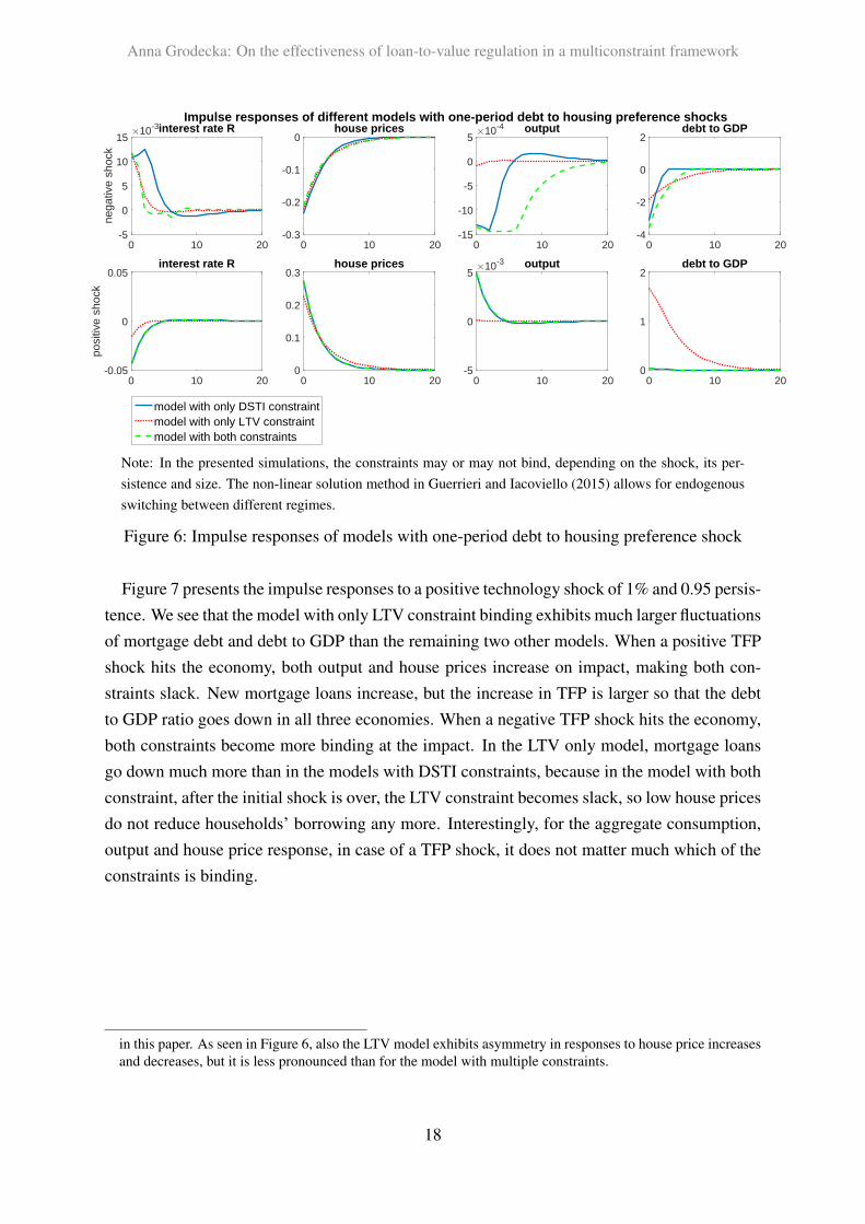
Figure 6 presents impulse responses of the three models to a persistent (ρ = 0.95) housingpreference shock of 5%: a negative shock (upper panel) and a positive shock (lower panel).8

Given the non-linear solution method, the responses to positive and negative shocks are asym-metric. A negative housing preference shock drives house prices and output down. Debt to

8 An extended version of this graph including Lagrangian multipliers is presented in Figure 13 in Appendix C.

16


Impulse responses of different models with one-period debt to exogenous shocks

0 10 20-1

-0.5

0debt to GDP

0 10 20-1.5

-1

-0.5

0×10-3 output

0 10 20-0.01

0

0.01

0.02house prices

0 10 20-0.01

-0.005

0

DS

TI s

hock

interest rate R

0 10 20-6

-4

-2

0debt to GDP

0 10 20-2

-1

0

1×10-3 output

0 10 20-0.4

-0.2

0

0.2house prices

0 10 20-0.1

-0.05

0

0.05

LTV

sho

ck

interest rate R

model with only DSTI constraintmodel with only LTV constraintmodel with both constraints

Note: In the presented simulations, the constraints may or may not bind, depending on the shock, its per-sistence and size. The non-linear solution method in Guerrieri and Iacoviello (2015) allows for endogenousswitching between different regimes.

Figure 5: Impulse responses of models with one-period debt to LTV and DSTI shocks

GDP goes down in all of the considered models, but mostly so in the model with both the DSTIand LTV constraint. In the multiconstraint model, after the shock, the LTV constraint becomesmore binding and the DSTI constraint slack at the impact. However, as house prices slowlygo back to the equilibrium level, the DSTI constraint becomes binding again (along with thebinding LTV constraint), driving down households’ borrowing and consumption and prolong-ing the downturn in the economy. When house prices increase, the LTV-only model suggest abig increase in the debt to GDP ratio, a multiple of the increase in house prices, which is in-consistent with the Swedish data. House prices and debt to income or GDP are increasing, butthe change in the indebtedness level does not exceed the pace of the house price increases. Themodel with both constraints and only DSTI constraint suggest a more sluggish increase in theindebtedness ratio as a response to the positive housing preference shock, given that in thesemodels, households’ borrowing cannot increase irrespectively of their income. The asymmetryin the responses to the housing preference shock is largest for the model with both constraints,suggesting a limited role of the constraints in the upturn, but amplifying role in the downturn.To obtain this result, I did not have to consider an extremely large shock, which suggests thatthe existence of multiple occasionally binding constraints amplifies the asymmetry in responsesto different shocks compared to models with one constraint only.9

9 A similar analysis is presented in Guerrieri and Iacoviello (2017) for the model with LTV constraint only, but fora shock that drives prices up and down by 20 percent, thus, a very large shock compared to the one considered

17


Impulse responses of different models with one-period debt to housing preference shocks

0 10 200

1

2debt to GDP

0 10 20-5

0

5×10-3 output

0 10 200

0.1

0.2

0.3house prices

0 10 20-0.05

0

0.05

posi

tive

shoc

k

interest rate R

0 10 20-4

-2

0

2debt to GDP

0 10 20-15

-10

-5

0

5×10-4 output

0 10 20-0.3

-0.2

-0.1

0house prices

0 10 20-5

0

5

10

15

nega

tive

shoc

k

×10-3interest rate R



Figure 6: Impulse responses of models with one-period debt to housing preference shock

Figure 7 presents the impulse responses to a positive technology shock of 1% and 0.95 persis-tence. We see that the model with only LTV constraint binding exhibits much larger fluctuationsof mortgage debt and debt to GDP than the remaining two other models. When a positive TFPshock hits the economy, both output and house prices increase on impact, making both con-straints slack. New mortgage loans increase, but the increase in TFP is larger so that the debtto GDP ratio goes down in all three economies. When a negative TFP shock hits the economy,both constraints become more binding at the impact. In the LTV only model, mortgage loansgo down much more than in the models with DSTI constraints, because in the model with bothconstraint, after the initial shock is over, the LTV constraint becomes slack, so low house pricesdo not reduce households’ borrowing any more. Interestingly, for the aggregate consumption,output and house price response, in case of a TFP shock, it does not matter much which of theconstraints is binding.

in this paper. As seen in Figure 6, also the LTV model exhibits asymmetry in responses to house price increasesand decreases, but it is less pronounced than for the model with multiple constraints.

18


Impulse responses of different models with one-period debt to TFP shocks

0 10 20-3

-2

-1

0debt to GDP

0 10 20-1

-0.5

0output

0 10 20-1

-0.5

0house prices

0 10 200

0.1

0.2

0.3

nega

tive

TF

P s

hock

interest rate R

0 10 20-1

-0.5

0

0.5debt to GDP

0 10 200

0.5

1

1.5output

0 10 200

0.5

1house prices

0 10 20-0.3

-0.2

-0.1

0

posi

tve

TF

P s

hock

interest rate R



Figure 7: Impulse responses to TFP shock

4. Model with Long-Term Debt

The model with long-term debt is a simple extension of the real business cycle model withshort-term debt presented in section 3. It differs from the one-period debt by the inclusion oflong-term debt contracts, the introduction of price rigidity due to the presence of retailers, andthe consideration of a central bank that sets the interest rates according to the Taylor rule. Debtcontracts in this economy are nominal.

4.1. Impatient households

Borrowers get utility from goods (cB) and housing (hB) consumption, as well as leisure.They provide labor (lB) to firms and borrow from savers subject to two constraints.

maxcBt ,h

Bt ,l

Bt ,sbt

E0

∞∑t=0

βB,t

(log cBt + jt log hBt −

lBtηB

ηB

). (15)

The budget constraint of borrowers is:

cBt + qt(hBt − (1− δh)hBt−1) +

(Rt−1 − 1 + κ)sbt−1πt

= bt + wBt lBt , (16)

19


where δh is the depreciation of the housing stock, qt denotes the housing price, Rt = 1 + it isthe interest rate, κ is the amortization rate, sbt is the stock of debt, πt is the inflation rate, bt isnew borrowing, and wBt l

Bt is labor income.

Debt evolves according to:

sbt =(1− κ)sbt−1

πt+ bt. (17)

Substituting for the evolution of the stock of debt, we get

cBt + qt(hBt − (1− δh)hBt−1) +

Rt−1sbt−1πt

= sbt + wBt lBt . (18)

As in the one-period version of the model, borrowing households face an LTV constraint,restricting their borrowing to a fraction of their collateral:

sbt ≤(1− κ)sbt−1

πt+mBqt(h

Bt − (1− δh)hBt−1) (19)

This formulation follows Finocchiaro et al. (2016) and Chen and Columba (2016) for Swedenand is similar to one of the formulations in Justiniano, Primiceri, and Tambalotti (2015), imply-ing that not all borrowers refinance their loans every period. The constraint emphasizes that theLTV regulation is applied to the flow of mortgages as defined in 17, which is consistent withthe lending practice in Sweden. The right hand side of equation 19 emphasizes that the collat-eral constraint only applies to adjustments in the housing stock of borrowers (new investmentin housing by borrowers), and not their total housing stock. Thus, in the disaggregated setup,we can interpret the constraint as applying only to a fraction of borrowers that actually readjusttheir mortgages in a given period.

Moreover, each period, a DSTI constraint imposes a limit on borrowing of households. Theirdebt service, including the amortization on existing loans, cannot exceed a certain fraction oftheir income, analogously to the one-period debt case.

sbt(Rt + κ− 1) ≤ DSTIwBt lBt (20)

Notice that the formulation in equation 20 implies that the DSTI constraint is applied to theflow of mortgages that is backed by the labor income of borrowers readjusting their loans in agiven period. Constraint 20 can be rewritten as:

bt(Rt + κ− 1) ≤ DSTIwBt lBt µt, (21)

where µt = btsbt

stands for the fraction of new/refinanced loans in a given period. If we didnot multiply equation 21 with the endogenously determined fraction of refinanced loans, the

20


flow of debt would be backed by all borrowers’ income and not only the income of borrowersactually taking out a new loan. Given the LTV constraint defined in 19, the formulation ofthe DSTI constraint as in 20 and 21 ensures that the LTV and DSTI constraints apply onlyto borrowers that readjust their loans in a given period. Arguably, one could assume that alllong-term loans are refinanced each period, but in practice, this does not happen.

The FOCs are (λLTVt is the Lagrangian multiplier on the LTV constraint and λDSTIt is theLagrangian multiplier on the DSTI constraint):w.r.t. sbt

1

cBt= βBEt

(Rt

cBt+1πt+1

)+ λLTVt − Et

βBλLTVt+1 (1− κ)

πt+1

+ λDSTIt (Rt + κ− 1) (22)

w.r.t. hBt

qtcBt

=jthBt

+ βBEt

((1− δh)qt+1

cBt+1

− (1− δh)λLTVt+1 mBqt+1

)+ λLTVt mBqt, (23)

w.r.t. lBtwBt = lBt

ηB−1cBt −DSTIcBt wBt λDSTIt , (24)

As in the one-period model, given the presence of inequality constraints, the model requiresthe Kuhn-Tucker conditions to hold if we are interested in determining the optimal behavior ofhouseholds.

The steady state expression for λLTV , denoted by the barred variable, can be found fromequation 23:

λLTV =qhB − βB qhB(1− δh)− jcB

mB qhB cB − βB(1− δh)mB qhB cB. (25)

The steady state expression for λDSTI , denoted by the barred variable, can be found fromequation 22:

λDSTI =1− βBR− λLTV cB + βBλLTV cB(1− κ)

(R + κ− 1)cB. (26)

As in the model version with one-period debt, if one of the Lagrangian constraints is 0, theterms linked to this constraint will drop out from the stated FOC and we will end up either in amodel with the LTV-constraint only, or in a model with DSTI-constraint only. For reasonableparameter values matching the presented economy to the Swedish data, the bindingness of bothconstraints cannot be excluded, just as in the one-period model case. I present the sensitivityof the values of Lagrangian multipliers to the calibration in section 4.5.1.

21


4.2. Patient households

Patient households maximize the utility function given by:

maxsbt,hSt ,l

St

E0

∞∑t=0

βt

(log cSt + jt log hSt −

lStηS

ηS

). (27)

The budget constraint of the patient household in real terms is:

cSt + qt(hSt − (1− δh)hSt−1) + sbt =

Rt−1sbt−1πt

+ wSt lSt , (28)

where sbt denotes the stock of loans, Rt is the interest rate, wSt lSt is labor income , qt denotes

the housing price.The First Order Conditions (FOCs) are:

w.r.t. sbt1

cSt= βEt

(1

cSt+1πt+1

)Rt, (29)

w.r.t. hStqtcSt

= βEt

((1− δh)qt+1

cSt+1

)+jthSt, (30)

w.r.t. lStwSt = lSt

ηS−1cSt . (31)

4.3. Firms

Firms are competitive profit maximizers and produce the intermediate good in the economyaccording to the production function:

yt = atlSt

αlBt

(1−α), (32)

where at denotes the productivity shock and the parameter α controls for savers’ labor share inthe production function.

Following Iacoviello (2005), I assume that retailers purchase the intermediate good from thefirms and produce a final good, imposing a markup X on the goods. This markup appears inthe FOC of the firms:

wSt =αytXtlSt

, (33)

wBt =(1− α)ytXtlBt

. (34)

The formulation of the retail sector follows Iacoviello (2005). Retailers are a source of price

22


stickiness in this economy, as they can only adjust their prices with probability 1− θ.

4.4. Monetary policy and market clearing conditions

The central bank follows the Taylor rule in the economy given by:

ln(Rt

R

)= ρRln

(Rt−1

R

)+ (1− ρR)

[ρπln

(πt−1π

)+ ρyln

(yt−1y

)]+ εR,t, (35)

where ρR, ρπ, ρy are the parameters determining central banks’ reaction to deviations from thesteady state interest rate level, inflation and output, and εR,t denotes an exogenous disturbance.This formulation is similar to the one used by the Riksbank, with the difference that in mymodel, the interest rate responds to the change in output, while in the Riksbank model, to thehours worked (see Adolfson, Laséen, Christiano, Trabandt, and Walentin, 2013).

The housing stock is fixed to 1:1 = hSt + hBt . (36)

The aggregate resource constraint is given by:

cSt + cBt + ih = yt, (37)

where ih = δhqt is investment in the housing stock.

4.5. Equilibrium and dynamic implications of multiple borrowingconstraints in the model with long-term debt

4.5.1. Calibration

The model is calibrated to the Swedish data (see Table 4). Housing depreciation rate ischosen to match the average LTV in the Swedish data: 65% (UC credit data). The values forDSTI and κ result in a debt to GDP ratio of 62%, between the value of 55% used in Finocchiaroet al. (2016) and the recent data indicator of 64% (for mortgage debt). It is assumed thatborrowers earn 20% of wage income in this economy. In Sweden, around 40 % of populationholds mortgages (UC credit data), but not all mortgage borrowers are credit-constrained asin the model. As discussed in section 2, a little bit more than half of new borrowers can bedefined as credit constrained. In the model, constraints apply both to the stock and flow ofmortgages, so setting the share of borrowers’ labor income to 20% as at the higher end ofcalibration, but other studies for Sweden (Finocchiaro et al., 2016 and Chen and Columba,2016) assume an even higher share of labor income earned by constrained borrowers (40% and67%). Savers’ preference for housing follows Finocchiaro et al. (2016) and Chen and Columba

23


Parameter Value Source/TargetβS savers’ discount factor 0.99 4%annual int. rateβB borrowers’ discount factor 0.93 high impatience level of borrowersδh housing depreciation rate 0.0076 average LTV of 65%mB LTV ratio for new loans 0.85 Swedish FSA limitDSTI DSTI ratio for households 0.25 with κ debt-to-GDP of 62%κ quarterly amortization rate 0.01 25 years amortizationα savers’ wage share 0.8 borrowers earn 20% of wage incomeηS savers’ labor supply aversion 2 Frisch labor supply elasticity of 1ηB borrowers’ labor supply aversion 2 Frisch labor supply elasticity of 1JS savers’ weight on housing 0.2 Finocchiaro et al. (2016)JB borrowers’ weight on housing 0.8 debt-to-GDP of 62% in the LTV modelθ degree of price stickiness 0.75 duration of price of 1 yearX price markup 1.01 4% annual markupρR interest rate inertia 0.833 Adolfson et al. (2013)ρπ central bank’s response to inflation 1.733 Adolfson et al. (2013)ρy central bank’s response to output 0.051 Adolfson et al. (2013)

Table 4: Benchmark calibration of the model

(2016). Borrowers preference for housing J ′′ is chosen to match the debt-to-GDP in the LTV-only economy to 62% and to ensure that both constraints can bind in equilibrium. The value 0.8is not far from 0.6 used in Finocchiaro et al. (2016). The remaining parameter values are fairlystandard. The debt to income of this calibrated economy accounts to 300%, slightly higher thanthe recent value of 250% observed in the 2015 UC data. The Taylor rule parameters correspondto the estimation results published by the Riksbank in Adolfson et al. (2013).

Figure 8 shows a range of values for borrowers’ impatience, governed by βB and their pref-erence for housing, JB for which the borrowing constraints are binding (for βB, the values0.8-0.99 were considered, for JB: 0.01 - 0.95). For both constraints to be binding, the level ofhousing preference of borrowing households has to be substantially high, and borrowers’ levelof impatience cannot be too low.

4.5.2. Equilibirum comparison

Table 5 presents equilibrium implications of four experiments: lowering LTV and DSTI by5% and increasing the interest rate and the amortization pace by 5%. In columns 2-4, the tablepresents the results of these experiments in the benchmark model with two constraints binding,a DSTI-only model and LTV-only model. The calibration is identical for these models andresults in a debt to GDP ratio of 62%. Let us first focus on the first three models presented in

24


0.8 0.82 0.84 0.86 0.88 0.9 0.92 0.94 0.96 0.98 1

-B

0

0.1

0.2

0.3

0.4

0.5

0.6

0.7

0.8

0.9

1

j

The sensitivity of the bindingness of the LTV constraint to -B and j in the model with multi-period debt

0

1

2

3

4

5

6

7

8

(a) λLTV as a function of βB and JB

0.8 0.82 0.84 0.86 0.88 0.9 0.92 0.94 0.96 0.98 1

-B

0

0.1

0.2

0.3

0.4

0.5

0.6

0.7

0.8

0.9

1

j

The sensitivity of the bindingness of the DSTI constraint to -B and j in the model with multi-period debt

0

1

2

3

4

5

6

7

(b) λDSTI as a function of βB and JB

Figure 8: The sensitivity of the bindigness of borrowing constraints in the model with long-termdebt

the table. Similarly to the one-period model, a decrease in the admissible LTV ratio has a bigeffect on the debt to GDP/income ratio in a model in which only LTV constraint is considered,but no effect on this ratio in the model with multiple constraints or with a DSTI constraintonly. In the multiconstraint framework, a stricter LTV limit raises house prices in equilibrium,while it lowers them in a LTV-only setup. Conversely, DSTI changes have only an effect onindebtedness in the models in which this constraint is present. When it comes to the effectsof equilibrium changes in the interest rate, the model with multiple constraints features thehighest house price sensitivity to changes in the interest rate. Across all the models, interest rateincreases lower the debt to GDP and house prices, slightly lowering the output. An increasein the amortization pace lowers household indebtedness in relation to the GDP, mostly so inthe LTV-only model. It has an ambiguous effect on house prices, and lowers the GDP in thelong run. Implementing any of the considered policies seems to be costly in terms of output,however, the output sensitivity to different measures is not too large. House prices react moststrongly to changes in the interest rates, across all three models.

Additionally, the fifth column of the table presents the experiment results for the ’Swedisheconomy’, which features a different calibration from the remaining models. ’The Swedisheconomy’ column aims at replicating the existing characteristics of the Swedish mortgage mar-ket in 2016 as presented in Figure 3, assuming that in equilibrium, 14% of borrowers are con-strained by both constraints at the same time (as in the benchmark economy), 26% of borrowersare constrained by DSTI-constraint only, and 60% of the borrowers are constrained by the LTVconstraint only.10 These shares are achieved by assuming that certain fractions of borrowers’

10 It is possible that another set of macroprudential policies would change the shares of borrowers in the economyconstrained by specific constraints, but the assessment of this effect is beyond the scope of this exercise that

25


income go to different types of borrowers. If, apart for the income shares, the calibration isleft unchanged and is as in the case of other three models, it results in a debt to GDP ratio ofover 120%, inconsistent with the data for Sweden. In order to achieve the target debt to GDPof 62% in the changed model with three different types of borrowers, I need to adjust someother parameters accordingly, which may have an impact on the equilibrium results of othervariables. In particular, the fraction of savers in economy, α, is assumed to be 0.861 insteadof 0.8, and κ 0.0125 instead of 0.01. Without this adjustment, the debt to GDP ratio of the’Swedish economy’ would be unrealistically high, but admittedly, the change may impact theeffects of experiments on some variables, particularly output. Among the borrowers, the sharesof labor income are assumed as follows in the ’Swedish economy’ case: borrowers bound byboth constraints earn 0.17 of borrowers’ income, borrowers bound by LTV constraint only 0.5of borrowers’ income, and the remaining borrowers’ income goes to borrowers constrained bythe DSTI constraint. Given the micro-distribution of borrowers in the Swedish economy in2011-2015, the fifth column of Table 5 gives us the most realistic picture of equilibrium effectsof different policies. Note that an equilibrium 5% change in the considered policies leaves thebindingness of Lagrangian multipliers unaffected. That is, given a 5% change in the policies,the long-run distribution of borrowers is unaffected (it might be that in the short run, someof the constraints become slack and I investigate this temporary effect looking at the impulseresponses to policy shocks in section 4.5.3.) The impact of LTV changes on the debt-to-GDPratio in this economy is substantially lowered compared to the LTV-only case (which is intu-itive given that only a fraction of borrowers is actually constrained by LTV-constraint only) andlowering the DSTI limit seems to be more effective, with less of a negative impact on equilib-rium house prices compared to a stricter LTV policy. In this experiment, higher amortizationpace has most effect on debt to GDP without big negative effects for house prices. Changingthe interest rate is effective in lowering debt to GDP ratios, but at the cost of substantially lowerhouse prices. While interpreting this results, it is important to bear in mind that in the presentedeconomy, borrowers have no option to circumvent the regulation, which may reduce the effec-tiveness of macroprudential regulation as recently discussed by Crowe, Dell’Ariccia, Igan, andRabanal (2013) and Cerutti, Claessens, and Laeven (2017). The equilibrium output effect of allthe presented policies is negligible.

4.5.3. Model dynamics

In the following, I present the short-run implications of multiple borrowing constraints ina model with long-term debt where these constraints are occasionally binding. Note that thesteady state ’Swedish economy’ excercise would be infeasible in the dynamic simulations with

should be thus treated as the assessment of the effectiveness of policies given the distribution of borrowersacross the constraints. Presented experiments maintain the bindingness of constraints in equilibrium.

26


Variable/Model Benchmark DSTI-only LTV-only ’Swedish economy’LTV ↓ 5%

Debt to GDP/income 0% 0% -7.88% -3.06%House prices +1.07% 0% -2.12% -3.17%

Borrowers’ housing stock +3.59% 0% -3.61% +0.50%Output -0.54% 0% -0.17% +0.09%

DSTI ↓ 5%Debt to GDP/income -5% -6.88% 0% -3.09%

House prices -1.50% +0.09% 0% -0.21%Borrowers’ housing stock -3.41% +1.27% 0% -2.60%

Output +0.15% -0.37% 0% -0.07%(R-1) ↑ 5%

Debt to GDP/income -2.45% -3.72% -1.82% -2.69%House prices -2.52% -2.17% -2.27% -2.24%

Borrowers’ housing stock -0.01% +1.97% +0.53% +1.50%Output -0.08% -0.30% -0.11% -0.15%

κ ↑ 5%Debt to GDP/income -2.43% -2.97% -4.22% -5.80%

House prices +0.58% +0.09% -0.16% -0.16%Borrowers’ housing stock +1.74% +0.37% +0.02% +6.09%

Output -0.12% -0.17% -0.03% -0.08%

Note: The ’Swedish economy’ calibration differs from the remaining three models in orderto maintain the same debt-to-GDP ratio in equilbrium. See more discussion in the text.

Table 5: Long-term effects of lower LTV, DSTI and higher interest rates in the models withlong-term debt

27


occasionally binding constraints. With three borrowers, each facing four possible regimes, theset of regimes to simulate would have to take into account 24 combinations of slack and/orbinding constraints for each of the borrowers. Thus, in the following simulations of bench-mark economy, there is only one type of borrower who may face two constraints, hence, themaximum number of considered regimes is four, as in the one-period debt case.

Figure 9 presents impulse responses to highly persistent 1% changes in the LTV and DSTIratios, as well as the amortization pace (ρ = 0.9999). In the model with long-term debt,LTV changes have an impact on debt to GDP ratio even in the benchmark model with bothconstraints, depicted with a green dashed line (through a different response of interest ratesand house prices compared to the model with one-period debt presented in Figure 5), but thisimpact is lower than in a model with LTV constraint only, presented with the red dotted line.This is because under lower LTV the DSTI constraint becomes slack, but alone the existence ofan additional constraint alters the behaviour of agents in economy, hence, the green dashed andred dotted line do not coincide. When it comes to DSTI changes, similarly to the model withone-period debt, they have an impact merely on the models with the DSTI constraint (solid blueline). Lower DSTI limit will make the DSTI constraint more binding and induce borrowers towork more, having a positive impact on output. In the short run, an increase in amortizationpace will only moderately lower the debt to GDP level and slightly decrease house prices. Italso has a positive effect on house prices through its incentivizing impact on borrowers’ laborsupply - faster amortization makes the DSTI constraint more binding on impact.

Figure 10 presents impulse responses to a persistent 5% change in the preference for hous-ing (ρ = 0.95). After a negative preference shock, house prices go down in all the models,and in the model with both constraints, the DSTI constraint becomes slack for a - hence thebenchmark model with two constraints and the model with LTV constraint only result in sim-ilar impulse responses. When house prices increase, the LTV-only model suggests the largestincrease in the debt ratio, as the household indebtedness in this model is tight to the collateralvalue of housing, irrespective of their income, which grows much less than housing prices aftera housing preference shock, causing only the muted response of the debt to GDP ratio in theeconomy with two borrowing constraints. This results in an asymmetry in responses to houseprices increases and decreases. The asymmetry is much more pronounced in the model withtwo constraints.11

Figure 11 presents impulse responses to a 1% monetary policy shock. When interest ratesgo down, house prices increase in all the models. The models considering the LTV constraintpredict a relatively moderate increase in the debt to GDP. Output increases mostly in the modelwith two constraints present: in this model, after the initial shock and slack DSTI constraint,rising house prices lead to a slack LTV constraint, but the DSTI constraint becomes more

11 An extended version of this graph including Lagrangian multipliers is presented in Figure 14 in Appendix D.

28


Impulse responses of different models with long-term debt to macroprudential shocks

0 10 20-1

-0.5

0debt to GDP

0 10 20-0.05

0

0.05

0.1output

0 10 20-0.1

-0.05

0

0.05house prices

0 10 20-10

-5

0

5

amor

tizat

ion

shoc

k ×10-3interest rate R0 10 20

-1.5

-1

-0.5

0debt to GDP

0 10 20-0.05

0

0.05output

0 10 20-0.4

-0.2

0

0.2house prices

0 10 20-10

-5

0

5

DS

TI s

hock

×10-3interest rate R0 10 20

-2

-1

0

1debt to GDP

0 10 20-0.04

-0.02

0

0.02output

0 10 20-1

-0.5

0

0.5house prices

0 10 200

5

10

LTV

sho

ck

×10-3interest rate R



Figure 9: Impulse responses of models with long-term debt to highly persistent LTV, DSTI andamortization rate shocks

binding.12 Households would like to borrow against the increasing value of their housing,but they cannot do so, unless their wage income increases as well, so in the model with twoconstraints, the borrowers increase their labor supply relatively more, driving the output up.Increasing interest rates lead to a fall in house prices and economic activity. Output in themodel with two constraints goes down only with a lag, as borrowers, trying to keep up theirborrowing, increase the labor supply on impact. House prices and debt to GDP seem to reactmore to an increase in the interest rates rather than decreases for small size shocks. The short-run impact of interest on house prices seems to be limited, but as the analysis in Table 5 shows,in the long run, changes in equilibrium interest rates tend to move house prices considerably.

Comparing the long-run and short-run simulations, we can try to address the question ofwhat could be a potential driver of increasing debt to income in countries like Sweden, whereborrowers face multiple borrowing constraints. As shown in Table 5, both macroprudentialstandards and interest level have a significant impact on the level of debt to GDP and house

12 More detailed impulse responses are presented in Figure 15 in Appendix D.

29


Impulse responses of different models with long-term debt to housing preference shocks

0 10 200

1

2debt to GDP

0 10 20-0.1

0

0.1

0.2output

0 10 200

1

2house prices

0 10 20-0.02

-0.01

0

0.01

posi

tive

shoc

k

interest rate R

0 10 20-3

-2

-1

0debt to GDP

0 10 20-0.1

-0.08

-0.06

-0.04

-0.02output

0 10 20-2

-1.5

-1

-0.5house prices

0 10 200

0.01

0.02

nega

tive

shoc

kinterest rate R



Figure 10: Impulse responses of models with long-term debt to housing preference shocks

prices in the economy. Among all the measures, changing the amortization pace and the DSTIstandards has most impact on debt to GDP in relation to house price changes. That indicates thateven without house price increases, a liberal amortization policy and DSTI policy could havecontributed to rising household indebtedness above the house price increases in the long run. InSweden, given the lack of the amortization requirement before 2016 and very low interest ratesfor a prolonged period, it was rather the combined effect of preference for low amortizationunder very low interest rates automatically relaxing the discretionary income constraint thatled to the increase in indebtedness.

Stricter LTV policies and higher interest rates are effective in reducing long-term debt-to-GDP ratio, but they also have a significant negative effect on house prices, unlike DSTI andamortization policies. In the short run, lowering LTV and DSTI is effective in reducing deb-to-GDP ratios, with stricter DSTI having a less negative impact on house prices and output thana stricter LTV policy. Amortization is also effective in reducing household debt without bignegative effects for output or house prices. Increasing interest rates in a multiple constrainteconomy lowers debt-to-GDP without a big negative effect on output. All the policy measuresthat are aimed at lowering indebtedness and linked to the bindingness of the DSTI constraint:amortization rate, interest rate, DSTI ratio, have a stabilizing effect on output after contrac-tionary shocks, since they make the DSTI constraint more binding and incentivize borrowersto increase their labor supply.

30


Impulse responses of different models with long-term debt to monetary policy shocks

0 10 20-1

-0.5

0

0.5debt to GDP

0 10 20-0.05

0

0.05

0.1output

0 10 20-0.04

-0.02

0

0.02house prices

0 10 20-0.04

-0.02

0

0.02inflation

0 10 20-1

0

1

2

inte

rest

rat

e in

crea

se

interest rate i0 10 20

-0.5

0

0.5

1debt to GDP

0 10 20-0.05

0

0.05

0.1output

0 10 20-0.02

0

0.02

0.04house prices

0 10 20-0.02

0

0.02

0.04inflation

0 10 20-1

0

1

inte

rest

rat

e de

crea

se interest rate i



Figure 11: Impulse responses of models with long-term debt to monetary policy shocks

5. Conclusion

In many countries, obtaining a mortgage requires not only a housing collateral, but alsosufficient repayment capability. An example of such a country is Sweden, known for highlevels of house prices and household indebtedness. In such a case, the question about theright tools affecting the debt ratios becomes an extremely important one. Many studies suggestlowering LTV ratios as an effective macroprudential tool, but they do so mostly using modelswhere the LTV constraint is the only considered constraint. This is not consistent with themortgage practice in some countries and may overstate the effectiveness of LTV as a policytool.

Swedish micro-data suggests that while a considerable share of borrowers is indeed con-strained by the LTV regulation, a non-negligible share is also constrained by a DSTI constraint,or by both constraints at the same time. If two constraints are potentially limiting the borrowingof households, we can think of four possible situations: either both constraints are binding, orDSTI constraint only, or LTV constraint only, or none of them. First, I construct a model withoccasionally binding constraints and establish that both constraints can bind at the same time.This allows me to study long-run implications of different policies in the LTV-only, DSTI-onlyand multiconstraint world. If borrowers are at both constraints, a tighter LTV regulation willbe ineffective in reducing households’ debt to GDP ratio in the long run as the ratio is pinned

31


down by a constant equal to the DSTI limit. Stricter LTV ratios will increase house pricesin equilibrium and not change the debt ratios at all. I show that this is true in a model withone-period debt and long-term debt, extending the intuition presented in a simple model to aNew-Keynesian setup, where I can study the effects of monetary policy in such an environment.Calibrating the model to match the distribution of borrowers across different constraints in theSwedish economy, I show that the effectiveness of LTV in influencing debt to GDP ratios isreduced substantially compared to an LTV-only economy, often used in studies assessing theimpact of this ratio. In the short run, house prices do not seem to be very sensitive to monetarypolicy shocks. Expansionary monetary policy has a much lesser impact on the debt to GDPratio in economies with the DSTI limit present. DSTI limit precludes leveraging only againstrising housing prices, with no support of the real economy, which may reduce rising house-hold indebtedness in cases when it is not accompanied by the wage and productivity growth.In general, the presence of multiple occasionally binding constraints amplifies asymmetries inthe business cycles, even for small shocks, which confirms the result obtained in Guerrieri andIacoviello (2017) for bigger fluctuations.

The model presented in this paper can be a useful tool for thinking about macropruden-tial policies in countries where multiple constraints are in place. The bindingness of differentconstraints is an empirical question and has to be studied for each country separately, but theSwedish case suggests that the mechanism presented in this paper can be relevant for policy-makers facing high indebtedness levels in the economy. In addition, it can explain why somemacroprudential measures may have only short-run effects, as found in the empirical literature.

References

ADOLFSON, M., S. LASÉEN, L. CHRISTIANO, M. TRABANDT, AND K. WALENTIN (2013):“Ramses II - Model Description,” Sveriges Riksbank Occasional Paper.

AKINCI, O. AND J. OLMSTEAD-RUMSEY (2017): “How effective are macroprudential poli-cies? An empirical investigation,” Journal of Financial Intermediation.

ALPANDA, S., G. CATEAU, AND C. MEH (2014): “A Policy Model to Analyze Macropruden-tial Regulations and Monetary Policy,” Bank of Canada Staff Working Papers.

ALPANDA, S. AND S. ZUBAIRY (2017): “Addressing household indebtedness: Monetary, fis-cal or macroprudential policy?” European Economic Review, 92, 47 – 73.

BANK OF SLOVENIA (2016): “Macroprudential recommendation for housing loans,” avail-able online at https://www.esrb.europa.eu/pub/pdf/other/201611004_Bank_of_Slovenia_notification_annex.en.pdf.

32

https://www.esrb.europa.eu/pub/pdf/other/201611004_Bank_of_Slovenia_notification_annex.en.pdf

https://www.esrb.europa.eu/pub/pdf/other/201611004_Bank_of_Slovenia_notification_annex.en.pdf


BIS (2017): “Debt service ratios for the private non-financial sector,” available online athttp://www.bis.org/statistics/tables_g.pdf.

CERUTTI, E., S. CLAESSENS, AND L. LAEVEN (2017): “The use and effectiveness of macro-prudential policies: New evidence,” Journal of Financial Stability, 28, 203–224.

CHEN, J. AND F. COLUMBA (2016): “Macroprudential and Monetary Policy Interactions in aDSGE Model for Sweden,” IMF Working Papers.

CROWE, C., G. DELL’ARICCIA, D. IGAN, AND P. RABANAL (2013): “How to deal with realestate booms: Lessons from country experiences,” Journal of Financial Stability, 9, 300 –319.

DE CARVALHO, F. A., M. R. CASTRO, AND S. M. A. COSTA (2014): “Traditional andmatter-of-fact financial frictions in a DSGE model for Brazil: the role of macroprudentialinstruments and monetary policy,” BIS Working Papers.

DIETSCH, M. AND C. WELTER-NICOL (2014): “Do LTV and DSTI caps make banks moreresilient?” .

EESTI PANK (2014): Requirements for housing loans, Eesti Pank.

EUROPEAN CENTRAL BANK (2005): “The Debt Servicing Burden of Euro Area Households- Some Macroeconomic and Microeconomic Evidence,” ECB Monthly Bulletin 2005.

EUROPEAN SYSTEMIC RISK BOARD (2015): “National competent or designatedauthorities for CRD IV/CRR instruments and current or future implementa-tion of macroprudential instruments (updated May 2015),” available online athttps://www.esrb.europa.eu/pub/pdf/other/Updated_table_

macroprudential_instruments_201505.pdf.

——— (2016): A Review of Macroprudential Policy in the EU in 2015, ESRB.

——— (2017): “National measures of macroprudential interest in the EU/EEA (updated29.09.2017) ,” Available online at https://www.esrb.europa.eu/national_policy/shared/pdf/overview_macroprudential_measures.xlsx.

FEDERAL RESERVE BOARD (2017): “Household Debt Service and Financial Obligations Ra-tios,” https://www.federalreserve.gov/releases/housedebt/.

FELL, J. (2015): “Credit flow restrictions: Implementation and coordination issues,” Availableonline at https://old.lb.lt/n25481/2_j_fell.pdf.

33

http://www.bis.org/statistics/tables_g.pdf

https://www.esrb.europa.eu/pub/pdf/other/Updated_table_macroprudential_instruments_201505.pdf

https://www.esrb.europa.eu/pub/pdf/other/Updated_table_macroprudential_instruments_201505.pdf

https://www.esrb.europa.eu/national_policy/shared/pdf/overview_macroprudential_measures.xlsx

https://www.esrb.europa.eu/national_policy/shared/pdf/overview_macroprudential_measures.xlsx

https://old.lb.lt/n25481/2_j_fell.pdf


FINANSINSPEKTIONEN (2004): “Finansinspektionen’s general guidelinesregarding creditrisk management in credit institutions and investment firms,” available online at http://www.fi.se/contentassets/814407dcdb3743d6a1b4d609ca8582d8/

fs0406eng.pdf.

——— (2010a): “Den svenska bolånemarknaden och bankernas kredit-givning,” available online at http://www.fi.se/contentassets/

5a3aebc15d4b430e88ef4da745eb9b37/bolanerapport_16feb102ny.

pdf.

——— (2010b): “Finansinspektionen’s general guidelines regarding limitations to thesize of loans collateralised by homes,” available online at http://www.fi.se/

contentassets/3239c506b3ca4196ac89ceb811d10605/fs1002_eng.

pdf.

——— (2016): “Regulations regarding mortgage amortisation require-ment,” Available online at http://www.fi.se/contentassets/

690c9d8430bd4961b6073dedf4f9105f/memo_amortisation_2016-16.

pdf.

FINOCCHIARO, D., M. JONSSON, C. NILSSON, AND I. STRID (2016): “Macroeconomiceffects of reducing household debt,” Sveriges Riksbank Economic Review.

GELAIN, P., K. J. LANSING, AND C. MENDICINO (2013): “House Prices, Credit Growth,and Excess Volatility: Implications for Monetary and Macroprudential Policy,” International

Journal of Central Banking, 9, 219–276.

GREENWALD, D. (2016): “The Mortgage Credit Channel of Macroeconomic Transmission,”Society for Economic Dynamics 2016 Meeting Papers.

GUERRIERI, L. AND M. IACOVIELLO (2015): “OccBin: A toolkit for solving dynamic modelswith occasionally binding constraints easily,” Journal of Monetary Economics, 70, 22–38.

——— (2017): “Collateral constraints and macroeconomic asymmetries,” Journal of Monetary

Economics, 90, 28–49.

HE, D., E. NIER, AND H. KANG (2016): “Macroprudential measures for addressing housingsector risks,” in Macroprudential policy, ed. by B. for International Settlements, Bank forInternational Settlements, vol. 86 of BIS Papers chapters, 117–122.

HULL, I. (2015): “The macro-financial implications of house price-indexed mortgage con-tracts,” Economics Letters, 127, 81–85.

34

http://www.fi.se/contentassets/814407dcdb3743d6a1b4d609ca8582d8/fs0406eng.pdf



http://www.fi.se/contentassets/5a3aebc15d4b430e88ef4da745eb9b37/bolanerapport_16feb102ny.pdf



http://www.fi.se/contentassets/3239c506b3ca4196ac89ceb811d10605/fs1002_eng.pdf



http://www.fi.se/contentassets/690c9d8430bd4961b6073dedf4f9105f/memo_amortisation_2016-16.pdf




IACOVIELLO, M. (2005): “House Prices, Borrowing Constraints, and Monetary Policy in theBusiness Cycle,” American Economic Review, 95, 739–764.

IACOVIELLO, M. AND M. PAVAN (2013): “Housing and debt over the life cycle and over thebusiness cycle,” Journal of Monetary Economics, 60, 221–238.

INTERNATIONAL MONETARY FUND (2017): Kingdom of the Netherlands. Macroprudential

policy framework, IMF.

JUSTINIANO, A., G. E. PRIMICERI, AND A. TAMBALOTTI (2015): “Credit supply and thehousing boom,” Federal Reserve Bank of New York Staff Reports.

LI, J. AND P. VAN SANTEN (2017): “Monetary Policy, Lending Standard, and Bank Riks-Taking: Evidence from the Swedish Mortgage Market,” in Essays in Empirical Finance, ed.by J. Li, Stockholm School of Economics, chap. 2, 83–118.

SVERIGES RIKSBANK (2014): From A to Z: the Swedish mortgage market and its role in the

financial system, Sveriges Riksbank.

A. Appendix A - Discretionary income vs DSTI limit

The KALP-calculation takes into account agent-specific characteristics, such as income, andsome lump-sum assumptions not linked to the individual’s income, such as the amount of theminimum consumption. It may be represented by a following equation (assuming long-termdebt):

(1− τl)WiLi + TR− C − (I(1− τh) + SR + κ)SBi −HE = 0, (38)

where τl are labor taxes, TR are transfers, C is the minimum consumption level, I is an averageinterest rate for a given bank, SR is the shock to the interest rate representing the ’stressed rate’scenario, τh is the interest rate tax deduction, κ is the amortization rate, SB the stock of debt,and HE are house expenses.

If we rewrite the KALP constraint, it will take the following form:

SBi =(1− τl)WiLi + TR− C −HE

I(1− τ) + SR + κ, (39)

The debt service to income ratio imposes a constraint similar to the KALP-constraint inSweden:

35


(I(1− τh) + κ)SB

(1− τl)WiLi= DSTI, (40)

where DSTI is the ratio set by the regulator.After rewriting, this constraint reads:

SBi = DSTI(1− τl)WiLiI(1− τh) + κ

, (41)

comparing to

SBi =(1− τl)WiLi

R(1− τ) + SR + κ+

TR− C −HEI(1− τ) + SR + κ

(42)

under the KALP constraint. We see that the DSTI constraint is a linear function of income,while the KALP constraint not, as the second part of equation 42 is applied lump-sum to allborrowers and does not depend on the individual’s characteristics. The lump-sum characteris-tics does not change the slope of the KALP-constraint, but it changes the intercept. Dependingon the values of DSTI , C, TR, HE and SR, either the DSTI or the KALP constraint can be asteeper function of household’s income. However, unless the DSTI ratio is set very high, usu-ally the KALP constraint will result in a borrowing limit being a steeper function of income,as demonstrated in Figure 12. Given that individual characteristics does not play a role in arepresentative agent world, in terms of modeling, DSTI and KALP constraints differ mostly bythe inclusion of additional lump-sum expenses in the constraint that do not affect the dynamicsof the model.

B. Appendix B - Simple Model with One-Period Debt

B.1. Patient households

Patient households get utility from goods and housing consumption, as well as leisure. Theyprovide labor to firms and loans to impatient households.

Patient households maximize the utility function given by:

maxbSt ,h

St ,L

St

E0

∞∑t=0

βt

(log cSt + jt log hSt −

lStηS

ηS

), (43)

where cSt denotes the consumption of the final good, jt is the marginal utility of housing subjectto random disturbances (following Iacoviello (2005), the disturbance is common to patient andimpatient households, and is a proxy for a housing demand or housing preference shock), hSt isthe housing stock held by savers, lSt denotes labor supply of patient households.

36


0 2 4 6 8 10 12 14 16 18 200

0.2

0.4

0.6

0.8

1

1.2

1.4

1.6

1.8

2Debt limit as a function of income given different borrowing constraints

gross income

debt

lim

it

DSTI=0.32KALPDSTI=0.5

Notes: The graph was generated under the following parameter values: I = 2,τh = 0.3,C = 0.2,TR =

0.1,HE = 0.1,SR = 3,κ = 2,τl = 0.3

Figure 12: Debt limit as a function of income given different borrowing constraints

The budget constraint of the patient household in real terms is:

cSt + qt(hSt − hSt−1) + bt = Rt−1bt−1 + wSt l

St , (44)

where bt denotes lending, Rt is the interest rate, wSt lSt is labor income , qt denotes the housing

price.The First Order Conditions (FOCs) are:

w.r.t. bt1

cSt= βEt

(1

cSt+1

)Rt, (45)

w.r.t. hStqtcSt

= βEt

(qt+1

cSt+1

)+jthSt, (46)

w.r.t. LStwSt = lSt

ηS−1cSt . (47)

37


B.2. Firms

Firms are competitive profit maximizers.The production function is:

yt = atlSt

αlBt

(1−α), (48)

where at denotes the productivity shock and the parameter α controls for savers’ labor share inthe production function.

Given the competitive environment, wages equal marginal product of labor.Entrepreneurs’ first order conditions

w.r.t. labor:wSt =

αytlSt, (49)

wBt =(1− α)yt

lBt. (50)

B.3. Market clearing conditions

The housing stock is fixed to 1:1 = hSt + hBt , (51)

where hS denotes savers’ housing stock and hB, the borrowers’ housing stock.The aggregate resource constraint is given by:

cSt + cBt = yt, (52)

where cS denotes savers’ consumption and cB borrowers’ consumption.

C. Appendix C - Impulse Responses for an Extended Set ofVariables in the Model with One-Period Debt

38


Impulse responses of different models with one-period debt to housing preference shocks

0 10 200

1

2Lag. mult. DSTI

0 10 200

0.5

1Lag. mult. LTV

0 10 20-0.2

0

0.2borrowers´ labor supply

0 10 200

1

2borrowers´ housing stock

0 10 200

1

2debt to GDP

0 10 20-5

0

5×10-3 output

0 10 200

0.2

0.4house prices

0 10 20-0.05

0

0.05

posi

tive

shoc

k

interest rate R0 10 20

0

0.2

0.4Lag. mult. DSTI

0 10 200

0.2

0.4Lag. mult. LTV

0 10 20-0.1

0

0.1borrowers´ labor supply

0 10 20-5

0

5borrowers´ housing stock

0 10 20-5

0

5debt to GDP

0 10 20-2

0

2×10-3 output

0 10 20-0.4

-0.2

0house prices

0 10 20-0.02

0

0.02

nega

tive

shoc

k

interest rate R



Figure 13: Impulse responses of models with one-period debt to housing preference shock

D. Appendix C - Impulse Responses for an Extended Set ofVariables in the Model with Long-Term Debt

39


Impulse responses of different models with long-term debt to housing preference shocks

0 10 20-2

0

2borrowers´ consumption

0 10 200

1

2borrowers´ housing

0 10 200

1

2borrowers´ labor

0 10 200

50

100Lag. mult. DSTI

0 10 200

10

20Lag. mult. LTV

0 10 200

1

2debt to GDP

0 10 20-0.2

0

0.2output

0 10 200

1

2house prices

0 10 20-0.02

0

0.02

posi

tive

shoc

k

interest rate R0 10 20

0

0.5


0 10 20-2

-1


0 10 20

-0.4

-0.2

0borrowers´ labor

0 10 200

5

10Lag. mult. DSTI

0 10 200

2

4Lag. mult. LTV

0 10 20-4

-2

0debt to GDP

0 10 20-0.1

-0.05

0output

0 10 20-2

-1

0house prices

0 10 200

0.01

0.02

nega

tive

shoc

k interest rate R



Figure 14: Impulse responses of models with long-term debt to housing preference shocks

40


Impulse responses of different models with long-term debt to monetary policy shocks

0 10 20-1

0


0 10 20-2

0


0 10 20-1

0

1borrowers´ labor

0 10 20-50

0

50Lag. mult. DSTI

0 10 200

5

10Lag. mult. LTV

0 10 20-1

0

1debt to GDP

0 10 20-0.1

0

0.1output

0 10 20-0.05

0

0.05house prices

0 10 20-0.05

0

0.05inflation

0 10 20-2

0

2

inte

rest

rat

e in

crea

se interest rate i0 10 20

-1

0


0 10 20-2

0


0 10 20-0.5

0

0.5borrowers´ labor

0 10 200

20

40Lag. mult. DSTI

0 10 200

5

10Lag. mult. LTV

0 10 20-1

0

1debt to GDP

0 10 20-0.1

0

0.1output

0 10 20-0.05

0

0.05house prices

0 10 20-0.05

0

0.05inflation

0 10 20-1

0

1

inte

rest

rat

e de

crea

se

interest rate i



Figure 15: Impulse responses of models with long-term debt to monetary policy shocks

41

Earlier Working Papers: For a complete list of Working Papers published by Sveriges Riksbank, see www.riksbank.se

Estimation of an Adaptive Stock Market Model with Heterogeneous Agents by Henrik Amilon

2005:177

Some Further Evidence on Interest-Rate Smoothing: The Role of Measurement Errors in the Output Gap by Mikael Apel and Per Jansson

2005:178

Bayesian Estimation of an Open Economy DSGE Model with Incomplete Pass-Through by Malin Adolfson, Stefan Laséen, Jesper Lindé and Mattias Villani

2005:179

Are Constant Interest Rate Forecasts Modest Interventions? Evidence from an Estimated Open Economy DSGE Model of the Euro Area by Malin Adolfson, Stefan Laséen, Jesper Lindé and Mattias Villani

2005:180

Inference in Vector Autoregressive Models with an Informative Prior on the Steady State by Mattias Villani

2005:181

Bank Mergers, Competition and Liquidity by Elena Carletti, Philipp Hartmann and Giancarlo Spagnolo

2005:182

Testing Near-Rationality using Detailed Survey Data by Michael F. Bryan and Stefan Palmqvist

2005:183

Exploring Interactions between Real Activity and the Financial Stance by Tor Jacobson, Jesper Lindé and Kasper Roszbach

2005:184

Two-Sided Network Effects, Bank Interchange Fees, and the Allocation of Fixed Costs by Mats A. Bergman

2005:185

Trade Deficits in the Baltic States: How Long Will the Party Last? by Rudolfs Bems and Kristian Jönsson

2005:186

Real Exchange Rate and Consumption Fluctuations follwing Trade Liberalization by Kristian Jönsson

2005:187

Modern Forecasting Models in Action: Improving Macroeconomic Analyses at Central Banks by Malin Adolfson, Michael K. Andersson, Jesper Lindé, Mattias Villani and Anders Vredin

2005:188

Bayesian Inference of General Linear Restrictions on the Cointegration Space by Mattias Villani

2005:189

Forecasting Performance of an Open Economy Dynamic Stochastic General Equilibrium Model by Malin Adolfson, Stefan Laséen, Jesper Lindé and Mattias Villani

2005:190

Forecast Combination and Model Averaging using Predictive Measures by Jana Eklund and Sune Karlsson

2005:191

Swedish Intervention and the Krona Float, 1993-2002 by Owen F. Humpage and Javiera Ragnartz

2006:192

A Simultaneous Model of the Swedish Krona, the US Dollar and the Euro by Hans Lindblad and Peter Sellin

2006:193

Testing Theories of Job Creation: Does Supply Create Its Own Demand? by Mikael Carlsson, Stefan Eriksson and Nils Gottfries

2006:194

Down or Out: Assessing The Welfare Costs of Household Investment Mistakes by Laurent E. Calvet, John Y. Campbell and Paolo Sodini

2006:195

Efficient Bayesian Inference for Multiple Change-Point and Mixture Innovation Models by Paolo Giordani and Robert Kohn

2006:196

Derivation and Estimation of a New Keynesian Phillips Curve in a Small Open Economy by Karolina Holmberg

2006:197

Technology Shocks and the Labour-Input Response: Evidence from Firm-Level Data by Mikael Carlsson and Jon Smedsaas

2006:198

Monetary Policy and Staggered Wage Bargaining when Prices are Sticky by Mikael Carlsson and Andreas Westermark

2006:199

The Swedish External Position and the Krona by Philip R. Lane

2006:200

Price Setting Transactions and the Role of Denominating Currency in FX Markets by Richard Friberg and Fredrik Wilander

2007:201

The geography of asset holdings: Evidence from Sweden by Nicolas Coeurdacier and Philippe Martin

2007:202

Evaluating An Estimated New Keynesian Small Open Economy Model by Malin Adolfson, Stefan Laséen, Jesper Lindé and Mattias Villani

2007:203

The Use of Cash and the Size of the Shadow Economy in Sweden by Gabriela Guibourg and Björn Segendorf

2007:204

Bank supervision Russian style: Evidence of conflicts between micro- and macro-prudential concerns by Sophie Claeys and Koen Schoors

2007:205

Optimal Monetary Policy under Downward Nominal Wage Rigidity by Mikael Carlsson and Andreas Westermark

2007:206

Financial Structure, Managerial Compensation and Monitoring by Vittoria Cerasi and Sonja Daltung

2007:207

Financial Frictions, Investment and Tobin’s q by Guido Lorenzoni and Karl Walentin

2007:208

Sticky Information vs Sticky Prices: A Horse Race in a DSGE Framework by Mathias Trabandt

2007:209

Acquisition versus greenfield: The impact of the mode of foreign bank entry on information and bank lending rates by Sophie Claeys and Christa Hainz

2007:210

Nonparametric Regression Density Estimation Using Smoothly Varying Normal Mixtures by Mattias Villani, Robert Kohn and Paolo Giordani

2007:211

The Costs of Paying – Private and Social Costs of Cash and Card by Mats Bergman, Gabriella Guibourg and Björn Segendorf

2007:212

Using a New Open Economy Macroeconomics model to make real nominal exchange rate forecasts by Peter Sellin

2007:213

Introducing Financial Frictions and Unemployment into a Small Open Economy Model by Lawrence J. Christiano, Mathias Trabandt and Karl Walentin

2007:214

Earnings Inequality and the Equity Premium by Karl Walentin

2007:215

Bayesian forecast combination for VAR models by Michael K. Andersson and Sune Karlsson

2007:216

Do Central Banks React to House Prices? by Daria Finocchiaro and Virginia Queijo von Heideken

2007:217

The Riksbank’s Forecasting Performance by Michael K. Andersson, Gustav Karlsson and Josef Svensson

2007:218

Macroeconomic Impact on Expected Default Freqency by Per Åsberg and Hovick Shahnazarian

2008:219

Monetary Policy Regimes and the Volatility of Long-Term Interest Rates by Virginia Queijo von Heideken

2008:220

Governing the Governors: A Clinical Study of Central Banks by Lars Frisell, Kasper Roszbach and Giancarlo Spagnolo

2008:221

The Monetary Policy Decision-Making Process and the Term Structure of Interest Rates by Hans Dillén

2008:222

How Important are Financial Frictions in the U S and the Euro Area by Virginia Queijo von Heideken

2008:223

Block Kalman filtering for large-scale DSGE models by Ingvar Strid and Karl Walentin

2008:224

Optimal Monetary Policy in an Operational Medium-Sized DSGE Model by Malin Adolfson, Stefan Laséen, Jesper Lindé and Lars E. O. Svensson

2008:225

Firm Default and Aggregate Fluctuations by Tor Jacobson, Rikard Kindell, Jesper Lindé and Kasper Roszbach

2008:226

Re-Evaluating Swedish Membership in EMU: Evidence from an Estimated Model by Ulf Söderström

2008:227

The Effect of Cash Flow on Investment: An Empirical Test of the Balance Sheet Channel by Ola Melander

2009:228

Expectation Driven Business Cycles with Limited Enforcement by Karl Walentin

2009:229

Effects of Organizational Change on Firm Productivity by Christina Håkanson

2009:230

Evaluating Microfoundations for Aggregate Price Rigidities: Evidence from Matched Firm-Level Data on Product Prices and Unit Labor Cost by Mikael Carlsson and Oskar Nordström Skans

2009:231

Monetary Policy Trade-Offs in an Estimated Open-Economy DSGE Model by Malin Adolfson, Stefan Laséen, Jesper Lindé and Lars E. O. Svensson

2009:232

Flexible Modeling of Conditional Distributions Using Smooth Mixtures of Asymmetric Student T Densities by Feng Li, Mattias Villani and Robert Kohn

2009:233

Forecasting Macroeconomic Time Series with Locally Adaptive Signal Extraction by Paolo Giordani and Mattias Villani

2009:234

Evaluating Monetary Policy by Lars E. O. Svensson

2009:235

Risk Premiums and Macroeconomic Dynamics in a Heterogeneous Agent Model by Ferre De Graeve, Maarten Dossche, Marina Emiris, Henri Sneessens and Raf Wouters

2010:236

Picking the Brains of MPC Members by Mikael Apel, Carl Andreas Claussen and Petra Lennartsdotter

2010:237

Involuntary Unemployment and the Business Cycle by Lawrence J. Christiano, Mathias Trabandt and Karl Walentin

2010:238

Housing collateral and the monetary transmission mechanism by Karl Walentin and Peter Sellin

2010:239

The Discursive Dilemma in Monetary Policy by Carl Andreas Claussen and Øistein Røisland

2010:240

Monetary Regime Change and Business Cycles by Vasco Cúrdia and Daria Finocchiaro

2010:241

Bayesian Inference in Structural Second-Price common Value Auctions by Bertil Wegmann and Mattias Villani

2010:242

Equilibrium asset prices and the wealth distribution with inattentive consumers by Daria Finocchiaro

2010:243

Identifying VARs through Heterogeneity: An Application to Bank Runs by Ferre De Graeve and Alexei Karas

2010:244

Modeling Conditional Densities Using Finite Smooth Mixtures by Feng Li, Mattias Villani and Robert Kohn

2010:245

The Output Gap, the Labor Wedge, and the Dynamic Behavior of Hours by Luca Sala, Ulf Söderström and Antonella Trigari

2010:246

Density-Conditional Forecasts in Dynamic Multivariate Models by Michael K. Andersson, Stefan Palmqvist and Daniel F. Waggoner

2010:247

Anticipated Alternative Policy-Rate Paths in Policy Simulations by Stefan Laséen and Lars E. O. Svensson

2010:248

MOSES: Model of Swedish Economic Studies by Gunnar Bårdsen, Ard den Reijer, Patrik Jonasson and Ragnar Nymoen

2011:249

The Effects of Endogenuos Firm Exit on Business Cycle Dynamics and Optimal Fiscal Policy by Lauri Vilmi

2011:250

Parameter Identification in a Estimated New Keynesian Open Economy Model by Malin Adolfson and Jesper Lindé

2011:251

Up for count? Central bank words and financial stress by Marianna Blix Grimaldi

2011:252

Wage Adjustment and Productivity Shocks by Mikael Carlsson, Julián Messina and Oskar Nordström Skans

2011:253

Stylized (Arte) Facts on Sectoral Inflation by Ferre De Graeve and Karl Walentin

2011:254

Hedging Labor Income Risk by Sebastien Betermier, Thomas Jansson, Christine A. Parlour and Johan Walden

2011:255

Taking the Twists into Account: Predicting Firm Bankruptcy Risk with Splines of Financial Ratios by Paolo Giordani, Tor Jacobson, Erik von Schedvin and Mattias Villani

2011:256

Collateralization, Bank Loan Rates and Monitoring: Evidence from a Natural Experiment by Geraldo Cerqueiro, Steven Ongena and Kasper Roszbach

2012:257

On the Non-Exclusivity of Loan Contracts: An Empirical Investigation by Hans Degryse, Vasso Ioannidou and Erik von Schedvin

2012:258

Labor-Market Frictions and Optimal Inflation by Mikael Carlsson and Andreas Westermark

2012:259

Output Gaps and Robust Monetary Policy Rules by Roberto M. Billi

2012:260

The Information Content of Central Bank Minutes by Mikael Apel and Marianna Blix Grimaldi

2012:261

The Cost of Consumer Payments in Sweden 2012:262 by Björn Segendorf and Thomas Jansson

Trade Credit and the Propagation of Corporate Failure: An Empirical Analysis 2012:263 by Tor Jacobson and Erik von Schedvin

Structural and Cyclical Forces in the Labor Market During the Great Recession: Cross-Country Evidence 2012:264 by Luca Sala, Ulf Söderström and AntonellaTrigari

Pension Wealth and Household Savings in Europe: Evidence from SHARELIFE 2013:265 by Rob Alessie, Viola Angelini and Peter van Santen

Long-Term Relationship Bargaining 2013:266 by Andreas Westermark

Using Financial Markets To Estimate the Macro Effects of Monetary Policy: An Impact-Identified FAVAR* 2013:267 by Stefan Pitschner

DYNAMIC MIXTURE-OF-EXPERTS MODELS FOR LONGITUDINAL AND DISCRETE-TIME SURVIVAL DATA 2013:268 by Matias Quiroz and Mattias Villani

Conditional euro area sovereign default risk 2013:269 by André Lucas, Bernd Schwaab and Xin Zhang

Nominal GDP Targeting and the Zero Lower Bound: Should We Abandon Inflation Targeting?* 2013:270 by Roberto M. Billi

Un-truncating VARs* 2013:271 by Ferre De Graeve and Andreas Westermark

Housing Choices and Labor Income Risk 2013:272 by Thomas Jansson

Identifying Fiscal Inflation* 2013:273 by Ferre De Graeve and Virginia Queijo von Heideken

On the Redistributive Effects of Inflation: an International Perspective* 2013:274 by Paola Boel

Business Cycle Implications of Mortgage Spreads* 2013:275 by Karl Walentin

Approximate dynamic programming with post-decision states as a solution method for dynamic 2013:276 economic models by Isaiah Hull

A detrimental feedback loop: deleveraging and adverse selection 2013:277 by Christoph Bertsch

Distortionary Fiscal Policy and Monetary Policy Goals 2013:278 by Klaus Adam and Roberto M. Billi

Predicting the Spread of Financial Innovations: An Epidemiological Approach 2013:279 by Isaiah Hull

Firm-Level Evidence of Shifts in the Supply of Credit 2013:280 by Karolina Holmberg

Lines of Credit and Investment: Firm-Level Evidence of Real Effects of the Financial Crisis 2013:281 by Karolina Holmberg

A wake-up call: information contagion and strategic uncertainty 2013:282 by Toni Ahnert and Christoph Bertsch

Debt Dynamics and Monetary Policy: A Note 2013:283 by Stefan Laséen and Ingvar Strid

Optimal taxation with home production 2014:284 by Conny Olovsson

Incompatible European Partners? Cultural Predispositions and Household Financial Behavior 2014:285 by Michael Haliassos, Thomas Jansson and Yigitcan Karabulut

How Subprime Borrowers and Mortgage Brokers Shared the Piecial Behavior 2014:286 by Antje Berndt, Burton Hollifield and Patrik Sandås

The Macro-Financial Implications of House Price-Indexed Mortgage Contracts 2014:287 by Isaiah Hull

Does Trading Anonymously Enhance Liquidity? 2014:288 by Patrick J. Dennis and Patrik Sandås

Systematic bailout guarantees and tacit coordination 2014:289 by Christoph Bertsch, Claudio Calcagno and Mark Le Quement

Selection Effects in Producer-Price Setting 2014:290 by Mikael Carlsson

Dynamic Demand Adjustment and Exchange Rate Volatility 2014:291 by Vesna Corbo

Forward Guidance and Long Term Interest Rates: Inspecting the Mechanism 2014:292 by Ferre De Graeve, Pelin Ilbas & Raf Wouters

Firm-Level Shocks and Labor Adjustments 2014:293 by Mikael Carlsson, Julián Messina and Oskar Nordström Skans

A wake-up call theory of contagion 2015:294 by Toni Ahnert and Christoph Bertsch

Risks in macroeconomic fundamentals and excess bond returns predictability 2015:295 by Rafael B. De Rezende

The Importance of Reallocation for Productivity Growth: Evidence from European and US Banking 2015:296 by Jaap W.B. Bos and Peter C. van Santen

SPEEDING UP MCMC BY EFFICIENT DATA SUBSAMPLING 2015:297 by Matias Quiroz, Mattias Villani and Robert Kohn

Amortization Requirements and Household Indebtedness: An Application to Swedish-Style Mortgages 2015:298 by Isaiah Hull

Fuel for Economic Growth? 2015:299 by Johan Gars and Conny Olovsson

Searching for Information 2015:300 by Jungsuk Han and Francesco Sangiorgi

What Broke First? Characterizing Sources of Structural Change Prior to the Great Recession 2015:301 by Isaiah Hull

Price Level Targeting and Risk Management 2015:302 by Roberto Billi

Central bank policy paths and market forward rates: A simple model 2015:303 by Ferre De Graeve and Jens Iversen

Jump-Starting the Euro Area Recovery: Would a Rise in Core Fiscal Spending Help the Periphery? 2015:304 by Olivier Blanchard, Christopher J. Erceg and Jesper Lindé

Bringing Financial Stability into Monetary Policy* 2015:305 by Eric M. Leeper and James M. Nason

SCALABLE MCMC FOR LARGE DATA PROBLEMS USING DATA SUBSAMPLING AND 2015:306 THE DIFFERENCE ESTIMATOR by MATIAS QUIROZ, MATTIAS VILLANI AND ROBERT KOHN

SPEEDING UP MCMC BY DELAYED ACCEPTANCE AND DATA SUBSAMPLING 2015:307 by MATIAS QUIROZ

Modeling financial sector joint tail risk in the euro area 2015:308 by André Lucas, Bernd Schwaab and Xin Zhang

Score Driven Exponentially Weighted Moving Averages and Value-at-Risk Forecasting 2015:309 by André Lucas and Xin Zhang

On the Theoretical Efficacy of Quantitative Easing at the Zero Lower Bound 2015:310 by Paola Boel and Christopher J. Waller

Optimal Inflation with Corporate Taxation and Financial Constraints 2015:311 by Daria Finocchiaro, Giovanni Lombardo, Caterina Mendicino and Philippe Weil

Fire Sale Bank Recapitalizations 2015:312 by Christoph Bertsch and Mike Mariathasan

Since you’re so rich, you must be really smart: Talent and the Finance Wage Premium 2015:313 by Michael Böhm, Daniel Metzger and Per Strömberg

Debt, equity and the equity price puzzle 2015:314 by Daria Finocchiaro and Caterina Mendicino

Trade Credit: Contract-Level Evidence Contradicts Current Theories 2016:315 by Tore Ellingsen, Tor Jacobson and Erik von Schedvin

Double Liability in a Branch Banking System: Historical Evidence from Canada 2016:316 by Anna Grodecka and Antonis Kotidis

Subprime Borrowers, Securitization and the Transmission of Business Cycles 2016:317 by Anna Grodecka

Real-Time Forecasting for Monetary Policy Analysis: The Case of Sveriges Riksbank 2016:318 by Jens Iversen, Stefan Laséen, Henrik Lundvall and Ulf Söderström

Fed Liftoff and Subprime Loan Interest Rates: Evidence from the Peer-to-Peer Lending 2016:319 by Christoph Bertsch, Isaiah Hull and Xin Zhang

Curbing Shocks to Corporate Liquidity: The Role of Trade Credit 2016:320 by Niklas Amberg, Tor Jacobson, Erik von Schedvin and Robert Townsend

Firms’ Strategic Choice of Loan Delinquencies 2016:321 by Paola Morales-Acevedo

Fiscal Consolidation Under Imperfect Credibility 2016:322 by Matthieu Lemoine and Jesper Lindé

Challenges for Central Banks’ Macro Models 2016:323 by Jesper Lindé, Frank Smets and Rafael Wouters

The interest rate effects of government bond purchases away from the lower bound 2016:324 by Rafael B. De Rezende

COVENANT-LIGHT CONTRACTS AND CREDITOR COORDINATION 2016:325 by Bo Becker and Victoria Ivashina

Endogenous Separations, Wage Rigidities and Employment Volatility 2016:326 by Mikael Carlsson and Andreas Westermark

Renovatio Monetae: Gesell Taxes in Practice 2016:327 by Roger Svensson and Andreas Westermark

Adjusting for Information Content when Comparing Forecast Performance 2016:328 by Michael K. Andersson, Ted Aranki and André Reslow

Economic Scarcity and Consumers’ Credit Choice 2016:329 by Marieke Bos, Chloé Le Coq and Peter van Santen

Uncertain pension income and household saving 2016:330 by Peter van Santen

Money, Credit and Banking and the Cost of Financial Activity 2016:331 by Paola Boel and Gabriele Camera

Oil prices in a real-business-cycle model with precautionary demand for oil 2016:332 by Conny Olovsson

Financial Literacy Externalities 2016:333 by Michael Haliasso, Thomas Jansson and Yigitcan Karabulut

The timing of uncertainty shocks in a small open economy 2016:334 by Hanna Armelius, Isaiah Hull and Hanna Stenbacka Köhler

Quantitative easing and the price-liquidity trade-off 2017:335 by Marien Ferdinandusse, Maximilian Freier and Annukka Ristiniemi

What Broker Charges Reveal about Mortgage Credit Risk 2017:336 by Antje Berndt, Burton Hollifield and Patrik Sandåsi

Asymmetric Macro-Financial Spillovers 2017:337 by Kristina Bluwstein

Latency Arbitrage When Markets Become Faster 2017:338 by Burton Hollifield, Patrik Sandås and Andrew Todd

How big is the toolbox of a central banker? Managing expectations with policy-rate forecasts: 2017:339 Evidence from Sweden by Magnus Åhl

International business cycles: quantifying the effects of a world market for oil 2017:340 by Johan Gars and Conny Olovsson l

Systemic Risk: A New Trade-Off for Monetary Policy? 2017:341 by Stefan Laséen, Andrea Pescatori and Jarkko Turunen

Household Debt and Monetary Policy: Revealing the Cash-Flow Channel 2017:342 by Martin Flodén, Matilda Kilström, Jósef Sigurdsson and Roine Vestman

House Prices, Home Equity, and Personal Debt Composition 2017:343 by Jieying Li and Xin Zhang

Identification and Estimation issues in Exponential Smooth Transition Autoregressive Models 2017:344 by Daniel Buncic

Domestic and External Sovereign Debt 2017:345 by Paola Di Casola and Spyridon Sichlimiris

The Role of Trust in Online Lending by Christoph Bertsch, Isaiah Hull, Yingjie Qi and Xin Zhang

2017:346

Sveriges Riksbank Visiting address: Brunkebergs torg 11 Mail address: se-103 37 Stockholm Website: www.riksbank.se Telephone: +46 8 787 00 00, Fax: +46 8 21 05 31 E-mail: [email protected]

Documents

Working paper nr