Economics Working Paper Series

Working Paper No. 1632

The Phillips multiplier

Regis Barnichon and Geert Mesters

January 2019

The Phillips Multiplier∗

Regis Barnichonpaq and Geert Mesterspbq

paq Federal Reserve Bank of San Francisco and CEPRpbq Universitat Pompeu Fabra, Barcelona GSE

January 11, 2019

Abstract

We propose a model-free approach for determining the inflation-unemployment trade-off faced by a central bank, i.e., the ability of a central bank to transform unemploymentinto inflation (and vice versa) via its interest rate policy. We introduce the Phillipsmultiplier as a statistic to non-parametrically characterize the trade-off and its dynamicnature. We compute the Phillips multiplier for the US, UK and Canada and documentthat the trade-off went from being very large in the pre-1990 sample period to beingsmall (but significant) post-1990 with the onset of inflation targeting and the anchoringof inflation expectations.

JEL classification: C14, C32, E32, E52.

Keywords: Marginal Rate of Transformation, Inflation-Unemployment trade-off, Dy-namic Multiplier, Instrumental variables, Phillips curve.

∗First draft: February 2018. We thank Oscar Jorda, Sylvain Leduc, Nicolas Petrosky-Nadeau, FrankSchorfheide, Adam Shapiro, Jim Stock, Paolo Surico, Mark Watson, Dan Wilson and participants at the2018 Annual SNDE Symposium, the 2018 IAAE Annual Meeting, the 2018 NBER Summer Institute andthe CEPR “Low Inflation and Wage Dynamics: Implications for Monetary Policy and Financial Stabilityconference at Banca Italia for helpful comments. The views expressed in this paper are the sole responsibilityof the authors and to not necessarily reflect the views of the Federal Reserve Bank of San Francisco or theFederal Reserve System. We thank Julien Champagne for graciously sharing his narrative monetary shocksseries for Canada. Mesters acknowledge support from the Spanish Ministry of Science and Technology:Grant ECO2015-68136-P, Marie Sklodowska-Curie Actions: FP7-PEOPLE-2012-COFUND Action grantagreement no: 600387, the Spanish Ministry of Economy and Competitiveness through the Severo OchoaProgramme for Centres of Excellence in R&D (SEV-2011-0075) and Fundacin BBVA scientific research grant(PR16-DAT-0043) on Analysis of Big Data in Economics and Empirical Applications.

1

1 Introduction

When I say there is a trade-off between inflation and unemployment, I do not mean [that there

is] a stable downward-sloping Phillips curve. [...] At its heart, the inflation-unemployment

trade-off is [...] a claim that changes in policy push inflation and unemployment in opposite

directions. Mankiw (2001)

The existence of an inflation-unemployment trade-off is at the core of monetary policy

making, because central banks rely on this trade-off to “transform” unemployment into

inflation (and vice-versa) through their interest rate policy. The ability of a central bank to

control inflation thus depends on the magnitude of this trade-off, or more precisely on the

central bank’s marginal rate of transformation (MRT) between unemployment and inflation.

The inflation-unemployment trade-off faced by policy makers, i.e., the MRT, is tradition-

ally inferred from a Phillips curve linking inflation to real activity or more generally from a

multivariate structural model involving a Phillips curve.

Unfortunately, this model-based approach suffers from two empirical challenges:1 (i)

specification uncertainty, and (ii) endogeneity issues. First, there is uncertainty about the

model’s relevant set of explanatory variables and about the appropriate dynamic lag structure

(e.g., Gordon (2011)). Second, endogeneity issues are pervasive. For the Phillips curve,

confounding from supply shocks, unobserved inflation expectations and measurement error in

the natural unemployment rate all lead to highly uncertain and potentially biased coefficient

estimates (e.g., Mavroeidis et al. (2014)).

In this paper, we avoid these empirical issues by proposing a model-free characterization

of the inflation-unemployment trade-off faced by policy makers. We introduce a statistic –the

Phillips multiplier– which is defined as the expected cumulative change in inflation caused

by a monetary shock that lowers expected unemployment by 1ppt. The Phillips multiplier

directly captures the central bank’s MRT across different horizons and we show that it can be

1By “model-based”, we designate any approach that proceeds in two-steps, which consist in (i) specifyingand estimating a Phillips curve as in the limited-information approach (e.g., Mavroeidis, Plagborg-Møller andStock (2014)) or a full system of structural equations as in a VAR or DSGE model (full information approach,e.g., Schorfheide (2011)), and (ii) inferring the policy-relevant trade-off from the estimated coefficients.

2

estimated by a simple instrumental variable regression where we regress cumulative inflation

on cumulative unemployment using monetary shocks as instruments.

Compared to earlier model-based characterizations of the central bank’s inflation-unemployment

trade-off, the Phillips multiplier offers a number of benefits. First, the Phillips multiplier is

a non-parametric characterization of the MRT: it captures how policy-induced changes in

unemployment affect inflation over different time scales, from short time scales (less than a

year), to medium term time scales (biennial), to longer time scales. As such, the Phillips

multiplier does not rely on any underlying model and is robust to model mis-specification.

Second, thanks to the use of instruments, the Phillips multiplier avoids the identification

issues that have plagued the Phillips curve literature; confounding factors and measurement

error.

Equipped with our Phillips multiplier, we revisit important lessons from the Phillips

curve literature in a robust and identified setting: (i) how large is the MRT? (ii) what are

the dynamics of the MRT, i.e. how fast and for how long can the central bank affect inflation

with a policy-induced change in unemployment? is the long-run MRT infinite, as implied by a

vertical long-run Phillips curve? (iii) has the MRT changed over time? Is the MRT smaller

in the more recent period, as suggested by the flattening of the Phillips curve (e.g., Ball

and Mazumder (2011)), or is that flattening spurious and instead due to mis-specification,

confounding from supply factors or to a mis-measured natural rate of unemployment? And if

the MRT is indeed smaller, is it because of better anchored inflation expectations or because

of a lower sensitivity of inflation to economic slack?

We compute the US Phillips multiplier using as external instruments the Romer and

Romer (2004) narratively identified monetary policy changes as well as the high frequency

identified monetary policy shocks pioneered by Kuttner (2001) and Gurkaynak, Sack and

Swanson (2005). Both identification schemes have their own advantages: the Romer and

Romer (2004) shocks cover a long sampling period (1969-2007), while the high frequency

shocks only cover the recent 1990-2008 period but are arguably more convincing in terms of

the exogeneity assumption.

3

The Phillips multiplier, and thus the MRT, has changed considerably between the pre-

and the post-1990 periods. In the pre-1990 period, the Phillips multiplier strictly increases

(in absolute value) with the horizon and diverges at longer horizons, pointing to an infinite

MRT. This is due to the inertial nature of inflation during this period: inflation reacts with

a one year lag to changes in unemployment, and the response of inflation is much more

persistent than that of unemployment. As a result, the Fed’s ability to steer inflation with

policy-induced unemployment movements is large.2

In the post-1990 period the situation is very different. While the Phillips multiplier

is still significantly different from zero in the medium run, it is much smaller and there

is no indication of divergence in the long run. The implication is that the Fed’s MRT is

substantially smaller, or in other words, that the Fed’s ability to steer inflation with policy-

induced unemployment movements has declined considerably.

This change in the MRT in the post-1990 period could be due to the anchoring of in-

flation expectations or to a change in the sensitivity of inflation to economic slack (holding

expectations constant). To separate these mechanisms, we show that the Phillips multiplier

can be written as the ratio of two separate dynamic multipliers: (i) a multiplier capturing

the MRT while holding inflation expectations constant, and (ii) a multiplier capturing the

degree of anchoring of inflation expectations.

We find that the anchoring of inflation expectations is responsible for most (if not all) of

the change in the MRT.3 Inflation expectations went from completely unanchored to almost

perfectly anchored. In the pre-1990 period, inflation expectations responded one-for-one

with inflation following monetary shocks, and this “zero-anchoring” implies a large long-run

MRT. Intuitively, any policy-induced transitory change in inflation feeds into inflation ex-

pectations, which then feeds into future inflation and so on, making the transitory change

in inflation persistent or even permanent. In the post-1990 period however, inflation expec-

2In the language of the Phillips curve literature, our non-parametric result corresponds to a close to ver-tical long-run Phillips curve, i.e., the absence of any long-run trade-off between inflation and unemployment:The Fed can only lower unemployment at the cost of an ever increasing rate of inflation.

3In contrast, the sensitivity of inflation to economic slack holding expectations constant is relatively flatbetween the two sample periods (at least given estimation uncertainty).

4

tations respond little to policy-induced changes in inflation, and this implies a much lower

MRT. Intuitively, with well-anchored inflation expectations, inflation movements have no

second-round effects through inflation expectations, and the overall inflation response to a

change in policy is smaller and less persistent.

To provide additional evidence for these findings, we study the MRT for two other ad-

vanced economies for which external instruments are available: the UK and Canada. These

two countries are of particular interest as both countries adopted (in respectively 1991 and

1992) an explicit inflation targeting mandate, which has been found to successfully anchor

inflation expectations (e.g., Levin, Natalucci and Piger (2004) and Gurkaynak, Levin and

Swanson (2010)). Thus, if the anchoring of inflation expectations leads to a large decline in

the MRT, this decline should also be apparent with UK and Canadian data. Using the nar-

ratively identified monetary policy shocks from Cloyne and Hurtgen (2016) and Champagne

and Sekkel (2017) we estimate the MRT using the Phillips multiplier, and we indeed find

that the MRTs for the UK and Canada are considerably smaller (and no longer diverging)

in the inflation targeting sample periods.

We see our model-free approach to characterize the MRT with the Phillips multiplier as

paralleling the literature on the fiscal multiplier, see the review of Ramey (2016). The fiscal

literature features two prominent ways to estimate the fiscal multiplier: (i) a model-based

approach based on DSGE or VAR models (where the multiplier is indirectly inferred from

the estimated parameters of the model) and (ii) a model-free approach where the multiplier

can be obtained directly from an IV regression involving the cumulative sum of output and

government spending, see Ramey and Zubairy (2018). While the Phillips curve literature

has so far relied on (i) by taking as a starting point the existence of a well-specified Phillips

curve relationship, our paper instead follows the non-parametric route pioneered by Ramey

and Zubairy (2018) in the fiscal literature.

In the context of the vast Phillips curve literature, a few papers have tried to characterize

the inflation-unemployment trade-off in an identified setting like us (King and Watson (1994),

Cecchetti and Rich (2001) and Benati (2015)) but always in a model-based context, typically

5

through structural VARs. Instead, the spirit of our approach is most closely related to Ball

(1994)’s non-parametric estimate of the sacrifice ratio based on narratively-identified dis-

inflationary episodes.

2 The MRT and the Phillips multiplier

In this section we introduce the Phillips multiplier as a statistic for characterizing the central

bank’s marginal rate of transformation (MRT) between unemployment and inflation: the

ability of a central bank to use its instrument (the policy rate) to transform unemployment

into inflation (or vice-versa).

In line with Mankiw (2001)’s definition of the inflation-unemployment trade-off, we define

the central bank’s average MRT between inflation and unemployment as the average change

in inflation caused by a change in policy that lowers the unemployment rate by 1ppt over

the next h periods:

MRTh �Bπt:t�hBit

����εit�1

{But:t�hBit

����εit�1

, h ¥ 0, (1)

where yt:t�h

� 1h

°hj�0 yt�j denotes the average value of some variable y over rt, t � hs and

Byt:t�h

Bit

���εit�1

denotes the marginal effect of an exogenous unit change εit in the central bank

instrument it on some average variable yt:t�h .

Since the average responses of π and u are computed over increasingly larger windows

rt, t�hs as h increases, MRTh captures the average marginal rate of transformation between

inflation and unemployment at different levels of time aggregation: from short time scales

(less than a year, h   4 using quarterly data), to medium term time scales (biennial, h � 8),

to longer time scales (e.g., h � 20). In this way, MRTh characterizes the dynamic nature of

the MRT faced by a central bank.

In this work we measure the average MRT directly using a statistic called the Phillips

6

multiplier. We define the Phillips multiplier as

Ph � Rπh{Ru

h, h � 0, 1, 2, . . . , (2)

where Rπj and Ru

j in (2) are the impulse responses of average inflation and unemployment

to a one-unit policy shock εit. Specifically, Rπh �

1h

°hj�0Rπ

j and Ruh �

1h

°hj�0Ru

j , with Ryj

the causal impulse response at horizon j of a variable y to a one-unit shock εit:

Ryh � Epyt�h|ε

it � 1, wtq � Epyt�h|ε

it � 0, wtq, (3)

where wt is a vector of control variable.4

The Phillips multiplier Ph is the natural statistical counterpart to our definition of the

average MRT: it measures how the forecast for inflation changes when a change in policy

lowers unemployment by 1ppt over the next h periods. The Phillips multiplier parallels

the concept of the government spending multiplier in the fiscal literature, see Ramey and

Zubairy (2018).5

A key advantage of the Phillips multiplier is that it can be estimated by an IV regres-

sion of cumulative inflation on cumulative unemployment using monetary policy shocks as

instruments. Importantly, one does not need to compute the impulse responses of inflation

and unemployment to a monetary shock.

Denote by ξt an instrumental variable for the policy shock εit. The following simple

proposition summarizes the result.

Proposition 1. The multiplier Ph can be estimated from the cumulative regression

h

j�0

πt�j � Phh

j�0

ut�j � w1tγh � et�h (4)

4While the impulse response of the average value of a variable is little unusual in the macroeconomicliterature, this is simply the cumulative impulse response of the variable discounted by the horizon.

5The government spending multiplier is often measured as the ratio of the cumulative impulse responsesof output and government spending, Ramey and Zubairy (2018).

7

where°hj�0 ut�j is instrumented by ξt and where wt is a vector of control variables.

Proof. See appendix.

The simple estimation strategy implied by (4) provides a number of advantages (see also

Ramey and Zubairy (2018)). First, standard errors for the multiplier are readily available.

Since the error terms et�h is likely to be serially correlated, we will adopt heteroskedasticity

and serial correlation robust standard errors. Second, instrument relevance can be easily

assessed, and we will report the heteroskedasticity and serial correlation robust F-statistic

of Olea and Pflueger (2013) to assess the strength of the first-stage.

3 Comparison with a model-based approach

In this section we compare our model-free characterization of the inflation-unemployment

trade-off with the traditional model-based approach. The latter consists of first estimating

a Phillips curve which may or may not be embedded in a larger structural model, and then

using the estimated coefficients to back out the policy-relevant trade-off. When compared

to this model-based approach, the Phillips multiplier offers a number of benefits.

First, by being defined directly from the impulse response functions of inflation and un-

employment to a monetary shock, the Phillips multiplier avoids the endogeneity issues that

have plagued the estimation of the Phillips curve, see Mavroeidis et al. (2014). In particular,

since monetary shocks are orthogonal to supply shocks and to the natural unemployment

rate u�t ,6 the Phillips multiplier will allow us to estimate the MRT (i) without bias from

confounding supply shocks and (ii) without any need for a measure of the natural unem-

ployment rate (because Ru�u�

h � Ruh). Note that these confounding factors have led to large

estimation uncertainty in the Phillips curve literature, see Mavroeidis et al. (2014).

Second, unlike the Phillips curve, the Phillips multiplier characterizes the MRT in a

non-parametric fashion. This provides robustness to mis-specification, which is particularly

attractive given the large uncertainty regarding the set of relevant explanatory variables to

6Under the common assumption that monetary policy is neutral under flexible prices (e.g., Galı (2015)).

8

include in the Phillips curve as well as the appropriate dynamic lag specification. See Gordon

(2011), King and Watson (1994) and the discussion in the appendix.

More generally, the coefficients of the Phillips curve alone may not be enough the char-

acterize the inflation-unemployment trade-off faced by the central bank. Indeed, since the

central bank influences real activity through its interest rate policy, the specification of the

(IS) curve may also matter. In fact while the MRT reduces the slope of the Phillips curve

in the basic New-Keynesian model (Galı (2015)), this is not a general result, and the MRT

typically depends on both the Phillips and the (IS) curve coefficients.7 We provide such an

example in the appendix. Since the (IS) curve suffers from similar specification and endo-

geneity issues as the Phillips curve (Fuhrer and Rudebusch (2004)), the estimation issues get

compounded. The non-parametric and identified nature of the Phillips multiplier, a statistic

specifically designed to characterize the MRT, allow us to side-step these issues.

4 Empirical estimates of the US Phillips multiplier

In this section we compute the Phillips multiplier for the US. Since our direct estimation of

the MRT relies on the existence of external instruments for exogenous changes in policy, the

sample period we consider is dictated by the availability of relevant instruments.

Our baseline estimates for the US are based on the Romer and Romer (2004) narrative

measure of exogenous monetary policy changes, which has the advantage of covering the

longest sample period (1969-2007). As an alternative, we will also rely on the recent high-

frequency identification (HFI) approach pioneered by Kuttner (2001) and use surprises in

fed funds futures prices around FOMC announcement as instruments for monetary shocks.8

For all specifications throughout this paper, we use quarterly data and include four lags

of inflation and unemployment as control variables wt in regression (4). Finally, as implied

7Intuitively, the central bank’s trade-off between inflation and unemployment depends on the relativespeed with which monetary policy affects unemployment versus inflation, and this relative speed depends onthe dynamic specifications of both the Phillips curve and the (IS) curve.

8See Gertler and Karadi (2015), Miranda-Agrippino (2016), Nakamura and Steinsson (2018) for morerecent examples of the use of HFI instruments to identify the effects of monetary policy.

9

by equation (3) we conduct all our analyses under a stationarity assumption.9

4.1 Full sample estimates

For our baseline estimate based on the Romer and Romer narrative shocks, the sample

covers 1969-2007 thanks to Tenreyro and Thwaites (2016)’s extension of the Romer and

Romer series. Inflation is measured as the (annualized) quarter-to-quarter change in the

PCE price level.

Figure 1 shows our baseline estimate for the Phillips multiplier for horizon h � 0 until

h � 20 and also reports the Olea and Pflueger (2013) F -stats from the first stage of the

instrumental variable regression (4).10 The F -statistics document to what extent the mone-

tary policy shocks are correlated with cumulative unemployment at horizon h. The F-stats

statistics are reasonable (around 10) for h between 8 and 14 quarters. After this period, the

F-statistics start to drop and the confidence bounds for the multiplier increase markedly.

The Phillips multiplier is initially indeterminate, but as time goes by Ph becomes nega-

tive, reaches about -2ppt after h � 12 quarters and diverges thereafter. Note that a large

(or infinite) long-run MRT implies that a transitory policy-induced change in unemployment

has a very persistent (or permanent) effect on inflation. With a large MRT, the Fed’s ability

to steer inflation with policy-induced unemployment movements is large. Equivalently, a

large MRT implies that the Fed could lower unemployment permanently only at the cost of

ever increasing inflation.11

To better understand the dynamic of the multiplier, we can separately study its individual

components, namely the impulse responses of average inflation and unemployment. Indeed,

the numerator Ruh and denominator Rπ

h of Ph are the impulse responses of the average

levels of inflation and unemployment over the next h period following a monetary policy

shock. Using local projections with instrumental variables (see Jorda (2005), Stock and

9We note that the main ideas of our methodology can be applied when a unit root is present.10As instruments, we use the three monthly Romer-Romer shocks in each quarter.11An infinite long-run MRT is reminiscent of the accelerationist Phillips curve of the 1970s where unem-

ployment was related to changes in inflation. We will come back to this point in the next section, where westudy the multiplier over different sample periods.

10

Watson (2018)), we can estimate the impulse responses of average inflation and average

unemployment from

πt:t�h � xtβπh � w1tγ

πh � eπh,t�h

ut:t�h � xtβuh � w1tγ

uh � euh,t�h

(5)

where xt is the fed funds rate instrumented with the Romer and Romer monetary shocks,

and the parameters βπh and βuh capture the effect of a one unit change in the policy rate on

average inflation and unemployment.

As shown in the right-column of Figure 1, the multiplier is initially indeterminate because

both unemployment and inflation respond with a lag to monetary policy, the well known

transmission lags of monetary policy (e.g., Svensson (1997)). Then, the multiplier builds

up (in absolute value) over time, because the response of inflation is delayed relative to

that of unemployment and because the response of inflation is more persistent than that of

unemployment: as average unemployment starts to mean-revert to its unconditional mean

at h � 10 (which ceteris paribus increases Ph � Rπh{Ru

h in absolute value), inflation remains

elevated and shows no sign of mean reversion. As a result, the multiplier keeps increasing

and diverges. The central bank can trigger a persistent (possibly permanent) change in

inflation at a finite unemployment cost, i.e., the MRT is large.

4.2 The US Phillips multiplier over time

Our results based on the full 1969-2007 sample mix very different policy regimes that blur

the interpretability of our results. In fact, a number of Phillips curve-based studies have

suggested substantial changes in the persistence of inflation as well as in the magnitude of

the inflation-unemployment trade-off; from the close to unit-root behavior of inflation in the

1970s (e.g., King and Watson (1994)) to the flattening of the Phillips curve in the post-1990

period (e.g., Ball and Mazumder (2011) and Blanchard (2016)).

In this section, we parallel the Phillips curve literature and study the evolution of the

Phillips multiplier over time, using our non-parametric and identified approach to re-assess

11

the evolution of the MRT over time. Importantly, unlike earlier Phillips-curve based studies,

our approach will allow us to discard confounding effects that could give the illusion of a

change in the MRT, notably a change in the variance contribution of supply shocks (which

varies the magnitude of the endogeneity bias), or mis-measured changes in the natural rate

of unemployment.12

To investigate a possible change in the Phillips multiplier since 1990, we draw on HFI

monetary surprises.13 Specifically, we follow Gertler and Karadi (2015) and consider changes

in Federal Funds futures rates (FF) around FOMC announcement dates as external instru-

ments.14 This measure is plausibly uncorrelated with other shocks because they are changes

across a short announcement window. To estimate the Phillips multiplier using HFI instru-

ments, we proceed as with the Romer-Romer shocks except that we add as control variables

the Greenbook forecasts for inflation and unemployment. This is to capture any changes in

the Federal Funds futures rates driven by the part of information set of the Fed that differs

from that of the market.

Since HFI monetary surprises are only available in the more recent period (1990-2008),15

we will report two sets of results to assess the evolution of the Phillips multiplier over time:

first, the Phillips multiplier estimated using the Romer-Romer narrative shocks over 1969-

1989, and second the Phillips multiplier estimated using the HFI monetary surprises over

1990-2008.

The results are shown in Figure 2. While the estimated multipliers are similarly indeter-

minate at short horizons, their behaviors differ markedly at longer horizons. The pre-1990

12For instance, if the natural rate of unemployment was over-estimated during the late 1990s, the unem-ployment gap would have been under-estimated (not small enough), leading to a downward-biased estimateof the slope of the Phillips curve.

13Unfortunately, the Romer and Romer narrative instruments cannot be used to study the MRT in themore recent period (such as post-1990), because they have very low relevance (low first-stage F-stats) andthus cannot be used to estimate the Phillips multiplier. See Ramey (2016) for a forceful account of thedifficulty of using the Romer-Romer shocks to learn about the effects of monetary policy in the post-1990period.

14Similar, as Gertler and Karadi (2015), we found that “FF4”, the three month ahead monthly Fed Fundsfutures, provided the best first-stage, and we will present results based on these instruments.

15We intentionally exclude the post-2008 period (the zero lower-bound period) during which forwardguidance played a more prominent role and the Fed started employing unconventional monetary tools thatcould have different effects than conventional monetary tools, see Swanson (2017).

12

multiplier clearly diverges with the horizon, while the post-1990 multiplier is roughly stable

at some small (but non-zero) long-run value. In other words, in the pre-1990 period, the

MRT is large: monetary policy can have a very persistent, perhaps permanent, effect on

inflation at a finite unemployment cost. In contrast, in the post-1990 period the MRT is

small (but significant) and does not diverge. Consequently, the multiplier is substantially

smaller in the post-1990 period with a multiplier at about -0.15 after 3-4 years, an order of

magnitude smaller than in the pre-1990 period.

To help understand this flattening of the multiplier, Figure 3 plots the impulse responses

of average inflation and unemployment in the two sample periods; pre-1990 and post-1990.

The reasons for the change in the multiplier are twofolds: for a given change in unemploy-

ment, the response of inflation (i) is a lot more muted (one order of magnitude smaller) in

the more recent period, and (ii) no longer displays inertia relative to unemployment and in

fact appears to mirror the impulse response of unemployment. In the next section, we will

explore to what extent the anchoring of inflation expectations can be behind this change in

the behavior of inflation and the MRT.

5 MRT and anchoring of inflation expectations

One hypothesis for the large change in the value of the MRT is a change in the anchoring of

inflation expectations. As noted by the Phillips curve literature, the anchoring of inflation

expectations could lead to inflation displaying less inertia and turning from an I(1) to an I(0)

process (e.g., Levin et al. (2004)),16 and thereby the re-emergence of a long-run inflation-

unemployment trade-off, i.e., to a non-vertical long-run Phillips curve (Akerlof, Dickens and

Perry (2000), Svensson (2015)).

16For instance, drifting (i.e., unanchored) inflation expectations can lead to a high share of wage indexationto past inflation, which will raise inflation persistence. In contrast, with anchored inflation-expectations,there should not be any wage indexation to past inflation, and inflation will display less inertia.

13

5.1 Decomposing the Phillips multiplier

We explore the change in the MRT by decomposing the Phillips multiplier into the ratio

of two separate dynamic multipliers: (i) a multiplier capturing the MRT holding inflation

expectations constant, and (ii) a multiplier capturing the degree of anchoring of inflation

expectations. We have

Ph �Kh

1�Ah, h � 0, 1, 2, . . . (6)

where Kh is the “expectation-augmented Phillips multiplier” and Ah is the “anchoring mul-

tiplier” which are defined as follows

Kh � Rπ�πe

h {Ruh

Ah � Rπe

h {Rπh

h � 0, 1, 2, . . . , (7)

The multiplier Kh is the dynamic non-parametric analog of κ, the slope of an expectation-

augmented Phillips curve (e.g., Coibion and Gorodnichenko (2015)), while Ah captures how

policy-induced inflation movements pass through to inflation expectations, and can be in-

terpreted as a dynamic measure of the degree of anchoring of inflation.17 Full anchoring of

inflation expectations corresponds to Ah � 0, while full pass-through of inflation to inflation

expectations implies Ah � 1. As we will see, the Ah parameter share close similarities with

the “α” parameter in the Phillips curve literature and Solow-Tobin tests of the natural rate

hypothesis, e.g., Gordon, Solow, Perry and Gordon (1970).18

Expression (6) makes clear that two factors can lead to a decline in the Phillips multiplier:

(i) a decline in the sensitivity of inflation to economic slack holding inflation expectations

constant (a decrease in Kh), and (ii) an increase in the anchoring of inflation expectations

17By focusing on the elasticity of inflation expectations to a shock, this measure is similar in spirit to othermeasures found in the literature, see e.g., Gurkaynak et al. (2010).

18In earlier Phillips curve regressions, α was traditionally the loading on past inflation meant to proxy forexpected inflation. In that context, a value of α close to one implies the existence of a (close to) unit-root ininflation and no long-run trade-off between inflation and unemployment. In addition to being non-parametricand properly identified with monetary shocks, our approach also differs from that literature, because we usea survey-based measure of inflation expectations and do not model inflation expectations with past inflation(and thereby avoid the Sargent (1971) critique of Solow-Tobin-type tests.).

14

(an increase in Ah).

As hÑ 8, K8 can be seen as capturing the cumulative direct effect of economic slack on

inflation, while A8 captures the cumulative second-round effects arising from the adjustment

of inflation expectations to inflation movements that then feed into inflation and in turn affect

inflation expectations further, etc... Given our interest in the decline in the long-run value

of the Fed’s MRT, we will let hÑ 8 to discuss two polar cases:

(i) With no anchoring of inflation expectations (A8 � 1), the MRT diverges as P8 ÝÑA8Ñ1

8. Intuitively, any policy-induced transitory change in inflation will feed into inflation

expectations, which will then feed into future inflation; making the transitory change in

inflation permanent (in the limit whereA8 Ñ 1).19 The central bank is able to engineer

large movements in inflation with small transitory movements in unemployment.

(ii) With some anchoring of inflation expectations, there is incomplete pass-through be-

tween inflation and inflation expectations, i.e., A8   1.20 This implies 0   P8   8,

provided that K8 is non-zero and finite. Intuitively, if after a policy change, inflation

expectations do not fully adjust to the overall change in inflation (incomplete pass-

through), movements in inflation have limited second-round effects and the cumulative

change in inflation is smaller. As a result, policy-induced unemployment movements

will generate smaller and only transitory inflation movements. More generally, the

stronger the anchoring of inflation expectations (the smaller A8), the smaller (in ab-

solute vaule) the long-run Phillips multiplier, i.e., the smaller the long-run MRT.

19In the language of the Phillips curve, the slope of the Phillips curve depends on inflation expectations,so that while the Phillips curve may be downward slopping in the short-run because current inflation deviatefrom inflation expectations, in the long-run, the slope of the Phillips curve tends to infinity if inflationexpectations full adjust to movements in inflation.

20An imperfect pass-through is clearly at odds with the full-information rational expectation. See Coibion,Gorodnichenko and Kamdar (2017) for consistent supporting evidence of departures from full-informationrational expectations, and Akerlof et al. (2000) for some implications of near-rational expectations on thelong-run slope of the Phillips curve.

15

5.2 Anchoring versus Flattening

To measure inflation expectations, we rely on the inflation forecasts of households from the

University of Michigan Survey of Consumers, and we use households’ forecast of price changes

over the next 12 months, consistent with Coibion and Gorodnichenko (2015)’s finding that

household forecasts appear to be a more relevant measure of inflation forecasts for the Phillips

curve than professional forecasts.21

Figure 4 plots the multipliers Kh and Ah, estimated for the pre-1990 and post-1990

samples using the Romer-Romer and HFI identification strategies. We can see that the

pre- and the post-1990 periods correspond precisely to cases (i) and (ii) discussed in the

above section, and the main reason for the change in the value of the MRT at medium

to long horizons is a drastic change in the anchoring of inflation expectations. The MRT

holding inflation expectations constant is relatively flat (Kpre�90h � Kpost�90

h ) between the two

sample periods (at least given estimation uncertainty), but the anchoring multiplier differs

markedly in the two periods. There is full pass-through of inflation to inflation expectations

(Ah � 1, h ¡ 10) in the pre-1990 period, and the Phillips multiplier Ph � Kh

1�Ahis large

and diverging.22. In contrast, for the post-1990 period, there is close to perfect anchoring

(Ah � 0, h ¡ 10), and we find P20 � K20 � �.15.

6 The Phillips multiplier across countries

In this final section, we estimate the Phillips multiplier for two other advanced economies

for which external instruments are available: the UK and Canada. These two countries

are of particular interest as an external validity test for our previous results. Indeed, both

countries adopted (in respectively 1991 and 1992) an explicit inflation targeting mandate,

which has been found to successfully anchor inflation expectations (e.g., Levin et al. (2004)

21We obtain similar results with median one-year ahead forecasts from the Survey of Professional Fore-casters or with longer-term 10-year ahead inflation expectations as estimated by the Board of Governors.

22In the language of the Phillips curve, the long-run slope of the Phillips curve is vertical and there is nolong-run trade-off between inflation and unemployment

16

and Gurkaynak et al. (2010)). Thus, if the anchoring of inflation expectations leads to a

large decline in the MRT, this decline should also be apparent with UK and Canadian data.

As measures of exogenous monetary policy changes, we rely on the narrative instruments

constructed by Cloyne and Hurtgen (2016) for the UK and by Champagne and Sekkel (2017)

for Canada. For the UK, inflation is measured as the (annualized) quarter-to-quarter change

in the retail prices index (excluding mortgage interest payments) following Cloyne and Hurt-

gen (2016). The sample period covers 1975-2007. For Canada, inflation is measured as the

(annualized) quarter-to-quarter change in the PCE price level and the sample period covers

1974-2014.

The left column of Figure 5 shows the estimated Phillips multiplier for the UK over two

sample periods, the pre-inflation targeting period (1975-1990, plain red line) and the inflation

targeting period (1991-2007, plain blue line) along with their 95 percent confidence bands.

Similarly, the right column shows the Phillips multiplier for Canada estimated over the pre-

inflation targeting 1975-1990 period (plain red line) and the inflation targeting 1992-2014

period (plain blue line).

The results are similar for the UK and Canada, and overall very similar to the US es-

timates. Consistent with the anchoring of inflation expectations leading to a large drop in

the MRT, the UK and Canada multipliers are considerably smaller (although still signifi-

cantly different from zero) and no longer diverging in the inflation targeting sample period.

In terms of magnitude, the long-run MRT appears largest in the UK, followed by Canada

and then the US. An interesting avenue for future research is to explore the significance

and possible reasons for this result, for instance whether it indicates a stronger anchoring

of inflation expectations in the US, or instead a lower Kh, i.e., a lower overall sensitivity of

inflation to economic slack (holding inflation expectations constant).

17

7 Conclusion

The inflation-unemployment trade-off faced by policy makers is traditionally inferred from

the coefficients of an estimated Phillips curve. However, such model-based approach is

fraught with specification and endogeneity issues. In this paper we propose a model-free

approach to directly characterize the central bank’s MRT with the Phillips multiplier ; the

cumulative change in inflation caused by a policy shock that raises unemployment by one

percentage point.

Using instruments for the US, UK and Canada, we revisit the main lessons of the Phillips

curve literature in a robust and identified setting. We find that (i) over short time scales

(less than a year) the MRT is indeterminate because of transmission lags in policy, (ii) over

medium time scales (biennial) the MRT is significantly negative, and (iii) the MRT went from

being very large in the pre-1990 sample period to being small (but still significant) in the

post-1990 period, i.e., during the onset of inflation targeting. Using inflation expectation

data for the US, we find that most of the change in the US MRT owes to the anchoring

of inflation expectations. In contrast, the overall sensitivity of inflation to economic slack

(holding inflation expectations constant) is not markedly lower between the two periods.

18

References

Akerlof, G. A., Dickens, W. T. and Perry, G. L.: 2000, Near-Rational Wage and PriceSetting and the Long-Run Phillips Curve, Brookings Papers on Economic Activity31(1), 1–60.

Ball, L.: 1994, What determines the sacrifice ratio?, Monetary policy, The University ofChicago Press, pp. 155–193.

Ball, L. and Mazumder, S.: 2011, Inflation dynamics and the great recession, BrookingsPapers on Economic Activity pp. 337–405.

Barth, M. and Ramey, V.: 2001, The cost channel of monetary transmission, NBERmacroeconomics annual 16, 199–240.

Benati, L.: 2015, The long-run Phillips curve: A structural VAR investigation, Journal ofMonetary Economics 76, 15–28.

Blanchard, O.: 2016, The phillips curve: Back to the ’60s?, American Economic Review106(5), 31–34.

Cecchetti, S. G. and Rich, R. W.: 2001, Structural estimates of the u.s. sacrifice ratio,Journal of Business & Economic Statistics 19(4), 416–427.

Champagne, J. and Sekkel, R.: 2017, Changes in Monetary Regimes and the Identificationof Monetary Policy Shocks: Narrative Evidence from Canada. Bank of Canadaworking paper: 2017-39.

Cloyne, J. and Hurtgen, P.: 2016, The macroeconomic effects of monetary policy: A newmeasure for the united kingdom, American Economic Journal: Macroeconomics8(4), 75–102.

Coibion, O. and Gorodnichenko, Y.: 2015, Is the Phillips Curve Alive and Well after All?Inflation Expectations and the Missing Disinflation, American Economic Journal:Macroeconomics 7(1), 197–232.

Coibion, O., Gorodnichenko, Y. and Kamdar, R.: 2017, The Formation of Expectations,Inflation and the Phillips Curve, NBER Working Papers 23304, National Bureau ofEconomic Research, Inc.

Fuhrer, J. C. and Rudebusch, G. D.: 2004, Estimating the Euler equation for output,Journal of Monetary Economics 51(6), 1133–1153.

Gali, J.: 2011, The Return Of The Wage Phillips Curve, Journal of the EuropeanEconomic Association 9, 436–461.

Galı, J.: 2015, Monetary policy, inflation, and the business cycle: an introduction to thenew Keynesian framework and its applications, Princeton University Press.

Gali, J. and Gertler, M.: 1999, Inflation dynamics: A structural econometric analysis,Journal of Monetary Economics 44, 195–222.

19

Gertler, M. and Karadi, P.: 2015, Monetary Policy Surprises, Credit Costs, and EconomicActivity, AEJ: Macroeconomics 7, 44–76.

Gordon, R. J.: 2011, The history of the phillips curve: Consensus and bifurcation,Economica 78, 10–50.

Gordon, R. J., Solow, R., Perry, G. and Gordon, R.: 1970, The recent acceleration ofinflation and its lessons for the future, Brookings Papers on Economic Activity1970(1), 8–47.

Gurkaynak, R. S., Levin, A. and Swanson, E.: 2010, Does inflation targeting anchorlong-run inflation expectations? evidence from the us, uk, and sweden, Journal of theEuropean Economic Association 8(6), 1208–1242.

Gurkaynak, Refet, S., Sack, B. and Swanson, E.: 2005, The Sensitivity of Long-TermInterest Rates to Economic News: Evidence and Implications for MacroeconomicModels, American Economic Review 95, 425–436.

Jorda, O.: 2005, Estimation and Inference of Impulse Responses by Local Projections, TheAmerican Economic Review 95, 161–182.

King, R. G. and Watson, M. W.: 1994, The post-war U.S. phillips curve: a revisionisteconometric history, Carnegie-Rochester Conference Series on Public Policy41, 157–219.

Kuttner, K. N.: 2001, Monetary policy surprises and interest rates: Evidence from the Fedfunds futures market, Journal of Monetary Economics 47(3), 523–544.

Levin, A. T., Natalucci, F. M. and Piger, J. M.: 2004, The macroeconomic effects ofinflation targeting, Review (Jul), 51–80.

Mankiw, N. G.: 2001, The Inexorable and Mysterious Tradeoff between Inflation andUnemployment, Economic Journal 111(471), 45–61.

Mavroeidis, S., Plagborg-Møller, M. and Stock, J. H.: 2014, Empirical Evidence onInflation Expectations in the New Keynesian Phillips Curve, Journal of EconomicLiterature 52, 124–188.

Miranda-Agrippino, S.: 2016, Unsurprising shocks: information, premia, and the monetarytransmission, Bank of England working papers 626, Bank of England.

Nakamura, E. and Steinsson, J.: 2018, High frequency identification of monetarynon-neutrality: The information effect, Quarterly Journal of Economics .

Olea, J. L. M. and Pflueger, C.: 2013, A robust test for weak instruments, Journal ofBusiness & Economic Statistics 31(3), 358–369.

Ramey, V.: 2016, Macroeconomic Shocks and Their Propagation, in J. B. Taylor andH. Uhlig (eds), Handbook of Macroeconomics, Elsevier, Amsterdam, North Holland.

20

Ramey, V. A. and Zubairy, S.: 2018, Government Spending Multipliers in Good Times andin Bad: Evidence from U.S. Historical Data, Journal of Political Economy 126.

Romer, C. D. and Romer, D. H.: 2004, A new measure of monetary shocks: Derivation andimplications, American Economic Review 94, 1055–1084.

Rudebusch, G. and Svensson, L. E.: 1999, Policy rules for inflation targeting, Monetarypolicy rules, University of Chicago Press, pp. 203–262.

Sargent, T. J.: 1971, A note on the accelerationist controversy, Journal of Money, Creditand Banking 3(3), 721–725.

Schorfheide, F.: 2011, Estimation and evaluation of dsge models: progress and challenges,Technical report, National Bureau of Economic Research.

Stock, J. and Watson, M.: 2018, Identification and estimation of dynamic causal effects inmacroeconomics using external instruments, The Economic Journal128(610), 917–948.

Svensson, L. E. O.: 1997, Inflation forecast targeting: Implementing and monitoringinflation targets, European Economic Review 41(6), 1111–1146.

Svensson, L. E. O.: 2015, The Possible Unemployment Cost of Average Inflation below aCredible Target, American Economic Journal: Macroeconomics 7(1), 258–296.

Swanson, E. T.: 2017, Measuring the effects of federal reserve forward guidance and assetpurchases on financial markets, Working Paper 23311, National Bureau of EconomicResearch.

Tenreyro, S. and Thwaites, G.: 2016, Pushing on a string: Us monetary policy is lesspowerful in recessions, American Economic Journal: Macroeconomics 8, 43–74.

21

Figure 1: The Phillips multiplier Ph — 1969-2007, RR

0 5 10 15 200

5

10

F-stat

Quarters

0 5 10 15 20−8

−6

−4

−2

0

2

ppt

Phillips multiplier

0 5 10 15 20

0

1

Ru h

Impulse Responses

0 5 10 15 20−4

−2

0

Rπ h

Quarters

Notes: Phillips multiplier estimated using Romer and Romer (RR) narrative monetary shocks as instruments.The sample is 1969q1-2007q4. Newey–West 95% confidence intervals displayed.

22

Figure 2: The Phillips multiplier Ph over time — RR/HFI

0 5 10 15 200

5

10

F-stat

Quarters

0 5 10 15 20

−4

−2

0

ppt

Pre-1990, RR

0 5 10 15 200

5

10

Quarters

0 5 10 15 20−0.6

−0.4

−0.2

0

0.2Post-1990, HFI

Notes: Left column: Phillips multiplier estimated using Romer-Romer (RR) monetary shocks over 1969q1–1989q4. Right column: Phillips multiplier estimated using High-Frequency Identified (HFI) monetary sur-prises (“FF4”, the three month ahead monthly Fed Funds futures) over 1990q1-2008q4. Newey–West 95%confidence intervals displayed.

23

Figure 3: IRs of average inflation and unemployment — RR/HFI

0 5 10 15 20

1

Ru h

Pre-1990, RR

0 5 10 15 20

−2

0

2

Rπ h

Quarters

0 5 10 15 20

0

1

Post-1990, HFI

0 5 10 15 20−0.4

−0.2

0

0.2

Quarters

Notes: Left column: Impulse responses for ut:t�h and πt:t�h computed using the Romer and Romer narrativemonetary shocks as instruments over 1969q1–1989q4. Right column: Impulse responses for ut:t�h and πt:t�h

computed using High-Frequency Identified (HFI) monetary surprises (“FF4”, the three month ahead monthlyFed Funds futures) over 1990q1–2008q4. 95% confidence intervals for the local projection estimates aredisplayed. For ease of comparison, the size of the monetary shock is set such that the impulse response ofaverage unemployment peaks at 1ppt in both cases.

24

Figure 4: Kh and Ah over time

0 5 10 15 20

−1

0

K

Pre-1990, RR

0 5 10 15 20

0

1

A

Quarters

0 5 10 15 20

−1

0

K

Post-1990, HFI

0 5 10 15 20

0

1

A

Quarters

Notes: Left column: The “expectation-augmented Phillips multiplier” (Kh) and the “anchoring multiplier”(Ah), estimated using Romer-Romer (RR) monetary shocks over 1969q1–1989q4. Right column: the samemultipliers estimated using High-Frequency Identified (HFI) monetary surprises (“FF4”, the three monthahead monthly Fed Funds futures) over 1990q1–2008q4. Newey-West 95% confidence intervals displayed.

25

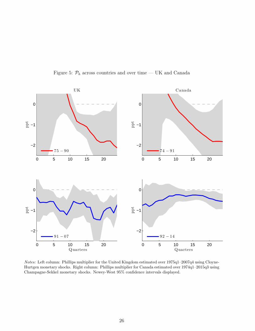
Figure 5: Ph across countries and over time — UK and Canada

0 5 10 15 20

−2

−1

0

ppt

UK

75 − 90

0 5 10 15 20

−2

−1

0

Quarters

ppt

91 − 07

0 5 10 15 20

−2

−1

0

ppt

Canada

74 − 91

0 5 10 15 20

−2

−1

0

Quarters

ppt

92 − 14

Notes: Left column: Phillips multiplier for the United Kingdom estimated over 1975q1–2007q4 using Cloyne-Hurtgen monetary shocks. Right column: Phillips multiplier for Canada estimated over 1974q1–2015q3 usingChampagne-Sekkel monetary shocks. Newey-West 95% confidence intervals displayed.

26