Working Paper No. 566

Caste and Wealth Inequality in India

by

Ajit ZachariasThe Levy Economics Institute

andVamsi Vakulabharanam

University of Hyderabad, Hyderabad

May 2009

Draft: Please do not cite or quote without permission.

The authors acknowledge the useful comments of the participants at theJuly 2007 ECINEQ conference in Berlin and the URPE/AEA meetings inJanuary 2008. Comments to: zacharia@levy.org;vamsi.vakul@gmail.com.

The Levy Economics Institute Working Paper Collection presents research in progress byLevy Institute scholars and conference participants. The purpose of the series is todisseminate ideas to and elicit comments from academics and professionals.

The Levy Economics Institute of Bard College, founded in 1986, is a nonprofit,nonpartisan, independently funded research organization devoted to public service.Through scholarship and economic research it generates viable, effective public policyresponses to important economic problems that profoundly affect the quality of life inthe United States and abroad.

The Levy Economics InstituteP.O. Box 5000

Annandale-on-Hudson, NY 12504-5000http://www.levy.org

Copyright © The Levy Economics Institute 2009 All rights reserved.

1

ABSTRACT

In this paper, we conduct the novel exercise of analyzing the relationship between overall

wealth inequality and caste divisions in India using nationally representative surveys on

household wealth conducted during 1991–92 and 2002–03. According to our findings,

the groups in India that are generally considered disadvantaged (known as Scheduled

Castes or Scheduled Tribes) have, as one would expect, substantially lower wealth than

the “forward” caste groups, while the Other Backward Classes and non-Hindus occupy

positions in the middle. Using the ANOGI decomposition technique, we estimate that

between-caste inequality accounted for about 13 percent of overall wealth inequality in

2002–03, in part due to the considerable heterogeneity within the broadly defined caste

groups. The stratification parameters indicate that the forward caste Hindus overlap little

with the other caste groups, while the latter have significantly higher degrees of overlap

with one another and with the overall population. Using this method, we are also able to

comment on the emergence and strengthening of a “creamy layer,” or relatively well-off

group, among the disadvantaged castes, especially the Scheduled Tribes.

Keywords: Caste; Inequality; Distribution of Wealth

JEL Classifications: D31, D63, J15

2

I. INTRODUCTION

It is widely acknowledged among social scientists that caste is a persistent determinant of

power, economic inequality, and poverty in contemporary India. Yet, economics

literature on caste relations in India is at best sparse, even as noneconomists (mainly

anthropologists and sociologists) have continued to make substantial contributions to the

overall literature on caste (e.g., Beteille [2007], Gupta [2000], and Srinivas [2000]). This

gap has been acknowledged recently and a call for greater attention to this axis of

differentiation has been made (Deshpande 2000). This, among other reasons, such as

better data availability, has given rise to an accelerated production of quantitative studies

on caste in the last few years (e.g., Barooah [2005], Deshpande [2001], Kojima [2006],

Munshi and Rosenzweig [2006], and Sundaram [2006]).

The quantitative studies on caste can be divided into two broad categories. First,

there are studies that have used either large surveys (mainly National Sample Survey

[NSS] consumption and National Family Health Surveys [NFHS]) or fieldwork-based

small sample surveys to show the evidence of caste differentials in consumption, income,

education, occupations, and development indices (e.g., see Deshpande [2001], Hasan and

Mehta [2006], Mehrotra [2006], Mohanty [2006], Srinivasan and Mohanty [2004], and

Sundaram [2006]). The near consensus in these studies is that the less privileged caste

groups tend to be worse off than the others on the measured indicators across the country,

although there are regional differences. Second, using large survey data, other studies

have employed the Blinder-Oaxaca decomposition (or modifications of this) to separate

the structural differences (e.g., geographical, discrimination-based) among households

from the differences in endowments (physical and human) in the market place (e.g., see

Barooah [2005] and Kojima [2006]) that create caste disparities. Barooah (2005), for

instance, using the National Council for Applied Economic Research (NCAER) survey

showed that about a third of the income differentials in India could be attributed to

discrimination in the market place. Using the NSS consumption surveys, Kojima showed

that both lower endowments of physical and human capital possessed by disadvantaged

groups, as well as different structures of income generation, contribute equally to the

disparities among caste groups. What is remarkable across these studies is the persistence

3

of systematic disparities among households across different caste groups over long

periods of time.

Our paper contributes to this literature by analyzing the relationship between

overall wealth inequality and caste divisions1 in India. There have been no studies on the

wealth disparities (as opposed to consumption or income disparities) within and among

caste groups on indicators and how these disparities contribute to the overall inequality in

India. Wealth inequality is an integral aspect of economic inequality among persons at a

given point in time, as well as across generations. Disparities in wealth can also translate

into disparities in economic security. For a substantial portion of the Indian population

that is dependent on agriculture, land is the major source of livelihood. Inequalities in the

quantity and fertility of land owned are a significant determinant of economic inequality

among households. Quality and quantity of schooling accessible to the children in urban

and semiurban areas can vary positively with household wealth.

The relationship between overall wealth inequality and caste is analyzed in this

study using the Yitzhaki decomposition or ANOGI2 (Yitzhaki 1994; Frick et al. 2004).

This allows us to separate the overall inequality into within-group and intragroup

components, rather than obtaining conditional average effects of social divisions via

regression-based decomposition methods such as the Oaxaca-Blinder method.

Furthermore, the overlapping parameters estimated using our chosen method permits the

distinction between caste-stratification and caste-inequality. This is especially important

in the context of ongoing debates in Indian political economy about the questions of

affirmative action and the so-called “creamy layer.”3

The remainder of the paper is organized as follows. Section II describes the data

and problems; we also outline the definitions of the caste groups. Section III describes the

1 We focus on caste for the purposes of this paper, although acknowledging that caste itself is a highly differentiated category. The 1911 census of India contained a far more detailed breakdown of caste groups than what is available in post-Independence data. Tabulations based on the 1911 census for Uttar Pradesh (the largest Indian state, then known as United Provinces) showed that among the 42 castes considered in the census, “each caste contained landless labourers, cultivators, as well as landlords” (Chaudhury 2004: 1990). Economic differentiation within castes is the rule rather than the exception, then and now. 2 ANOGI stands for “Analysis of Gini.” 3 The “creamy layer” refers to the emergence of an economically well-off group within castes whose average member is worse-off relative to the rest of the population.

4

patterns of wealth disparities among caste groups. The subsequent section (IV) presents

the decomposition results. Section V concludes.

II. DATA AND DEFINITIONS

The data used in this paper are from the two rounds of the All India Debt and Investment

Survey (AIDIS) conducted in 1991–92 and 2002–03. Wealth is computed as the total

household assets net of the indebtedness. Household assets are defined as “physical assets

like land, buildings, livestock, agricultural machinery and implements, non-farm business

equipment, all transport equipment, durable household goods, and financial assets like

dues receivable on loans advanced in cash or in kind, shares in companies, and

cooperative societies, banks, etc., national saving certificates and the like, deposits in

companies, banks, post offices, and with individuals” (NSS 2005: 5). Debt is defined as

cash loans payable. In the absence of a better deflator, the Consumer Price Index for

agricultural workers is used to make the 1991 and 2002 rural wealth values comparable

across time. Similarly, the Consumer Price Index for industrial workers is used to make

urban wealth values comparable across time.

The unit of analysis for the whole paper is the household adjusted for its size.

That is, the household weight is multiplied by the household size to obtain a distribution

among persons. We use per capita wealth—household wealth divided by household

size—as the measure of wealth. The implicit equivalence scale assumed here is that there

are no “economies of scale” associated with wealth. (For the relative advantages and

disadvantages of using this method for Indian wealth data, see Jayadev, Motiram, and

Vakulabharanam [2007].)

The definitions of caste groups are completely dictated by the data and do not

adequately reflect the complex and layered reality of caste in India. Both the AIDIS

rounds allow for the classification of the entire population into three groups, viz., the

Scheduled Castes or the “Dalits” (SC), Scheduled Tribes or the “Adivasis” (ST), and

everyone else whom we call Other Communities (OC). We term this classification

“Scheme I.” The 2002–03 survey introduced the additional category of Other Backward

5

Classes (OBC).4 In addition, the category of religion was also enumerated. Cross-

tabulating caste and religion allows for the separation of OC into three distinct groups:

OBC; Hindus who are not SC, ST, or OBC whom we call Hindu forward castes (FC); and

non-Hindus (NH) who are not SC, ST, or OBC. The 2002–03 survey, therefore, allows

for the classification of the population into five caste groups. We term this classification

“Scheme II.” It should be noted that the SC and ST individuals might belong to any

religion.

A brief note is in order regarding the category of caste. Caste in India is defined

differently along the “Varna” and the “Jati” schemes. The Varna scheme has four broad

groups—Brahmins, Kshatriyas, Vis, Sudras—and those people outside the Varna

scheme, ranked in a descending order of ritual status. Brahmins were traditionally

associated with the priestly and scholarly community. Kshatriyas were the ruling groups.

Vis were associated with those groups associated with trading, moneylending, and

retailing. Sudras were the peasants and artisans. Among those outside the Varna scheme,

the so-called “untouchables” (the present day Dalits) were mostly associated with the

rural, landless laboring community and the tribal groups (the present day Adivasis) were

associated with those living on the fringes of or outside the settled agricultural society. It

is generally agreed upon that this is a textual scheme defined by the Brahmins.

The Jati scheme is very different. There are thousands of Jati groups that vary

spatially and temporally in terms of their ritual rankings, socioeconomic status, and

occupations. It is also important to recognize that the caste system functions on the

ground along different Jati orderings, thus creating a bewildering variety of them, as well

as a system that cannot be neatly captured by structural and closed systems that can be

deployed across space and time (for important renditions of the caste system, see Dumont

[1970], Chatterjee [1993], and Gupta [2000]). Similarly, while certain occupations are

traditionally associated with certain caste groups (especially Jati groups), this relation too

is problematic given the significant flux in this relationship over time. However, it has

generally been the case that those outside the Varna scheme have tended to be

4 The determination of disadvantaged groups (OBCs) was made according to the 1931 census. Many changes have occurred since in the socioeconomic status of these groups, but this category does not reflect these changes, in part because subsequent censuses have not collected information on caste. The need for a new caste-based census is the subject of a heated debate in contemporary politics and the public sphere.

6

concentrated in the menial occupations, and this relationship also needs careful

examination in our times to see if independent India has been able to shake off some of

the entrenched caste-based hierarchies. We therefore use the categories (Varna-based)

that are available in the surveys to make broad decomposition analyses of the overall

inequality in India.

We further separate the rural areas from the urban, as we believe that the wealth

accumulation and income generation dynamics vary significantly across this sectoral

division.

The problems associated with the wealth data in the surveys are identified in the

literature (see, for example, Subramaniam and Jayaraj [2006] and Jayadev, Motiram, and

Vakulabharanam [2007]). They deserve a brief recapitulation. There are basically four

kinds of problems with these data. First, wealth distributions tend to be concentrated at

the very top end. Unless a special effort is made to oversample the very wealthy, the

concentration of wealth tends to be underrepresented. This will artificially reduce the

overall inequality. Second, there is a tendency among people of all wealth groups to

underreport their wealth holdings. This tendency to underreport is exacerbated as wealth

holdings rise. This will widen the gap between those with close to no wealth and those

that have some wealth. Third, the reported assets may not be correctly valued. It has been

found in India that the reported values of even recent transactions tend to be lower than

the market values. Given the lack of proper wealth-based deflators, the wealth values that

are analyzed can be somewhat off the mark. Fourth, there is a tendency to hide

illegitimate wealth that will lead to undercounting of the assets owned by the wealthy.

Finally, there is a strong tendency to underreport liability or debt. These problems add up

to a state wherein populations belonging to the wealthier groups (more prevalent among

the non-SC/ST population) appear to hold lower wealth than they actually have and the

less wealthy groups (especially the SC/ST groups) report higher wealth than they have.

This will certainly reduce the overall inequality, but it will also reduce the between-caste

inequality figures. These problems might be reflected in our findings.

7

III. CASTE DISPARITIES IN WEALTH

Most studies of economic inequality in India have used consumption expenditure as the

indicator of economic status. Our choice of wealth as the indicator of economic status

would be superfluous if consumption expenditure and wealth are distributed similarly

across individuals. While the two are correlated, the ranks of individuals in the two

distributions can be quite different (table 1). If all individuals in a given quintile of one

distribution also belong to the same quintile of the other distribution, then every number

on the principal diagonal of the matrix shown in table 1 will be equal to twenty and every

off-diagonal number will be equal to zero. Inspection of the table shows that the largest

number occurs at the intersection of the top quintiles of the two distributions. This

number indicates that only about half (10.4/20 = 52 percent) of those in the top quintile of

wealth distribution were also in the top quintile of consumption expenditure. In other

quintiles, at least two-thirds of individuals in a given quintile of wealth distribution were

located in a different consumption quintile, with the third quintile showing the weakest

correlation in rankings.5

5 Indeed, the picture can be more complicated than suggested by the table since we expect rankings of individuals within quintiles also to be different, depending on whether wealth or consumption is used as the ranking variable.

8

Table 1. Joint Distribution of Wealth and Consumption, 2002 Consumption

Wealth 1991 q1 q2 q3 q4 q5

q1 7.2 4.8 3.4 2.4 2.2q2 5.5 5.2 4.2 3.0 1.9q3 3.8 4.7 4.7 4.0 2.8q4 2.6 3.6 4.7 5.1 4.0q5 0.9 1.7 3.0 5.4 9.1

Total 20.0 20.0 20.0 20.0 20.0 2002

q1 7.3 4.8 3.7 2.4 1.4q2 5.8 5.1 4.2 3.0 1.5q3 3.9 4.6 4.7 4.2 2.5q4 2.3 3.7 4.6 5.3 4.2q5 0.7 1.8 2.8 5.1 10.4

Total 20.0 20.0 20.0 20.0 20.0Note: Consumption is measured as per capita consumption expenditures (MPCE), i.e., total household consumption expenditures divided by the number of persons in the household.

Let us now turn to examine disparities in wealth and wealth distributions among

caste groups. Since comparisons between the two years are possible only with the six-

group schema (ST, SC, and OC), differentiated by their rural versus urban location, we

begin with a consideration of the estimates shown in the upper panel of table 2. Between

1991 and 2002, the relatively disadvantaged groups (SC and ST) experienced rates of

growth in mean per capita wealth that are better than the majority group in both the urban

and rural areas. However, the medians tell a different story, especially for the ST. The

wealth of the average person in that group rose only 7 percent in the urban areas (as

compared to 42 percent for the urban OC) and 21 percent in the rural areas (versus 25

percent increase for the rural OC). In contrast, the average SC person experienced a

robust increase in wealth of approximately 40 percent over the same period in both the

urban and rural areas.

9

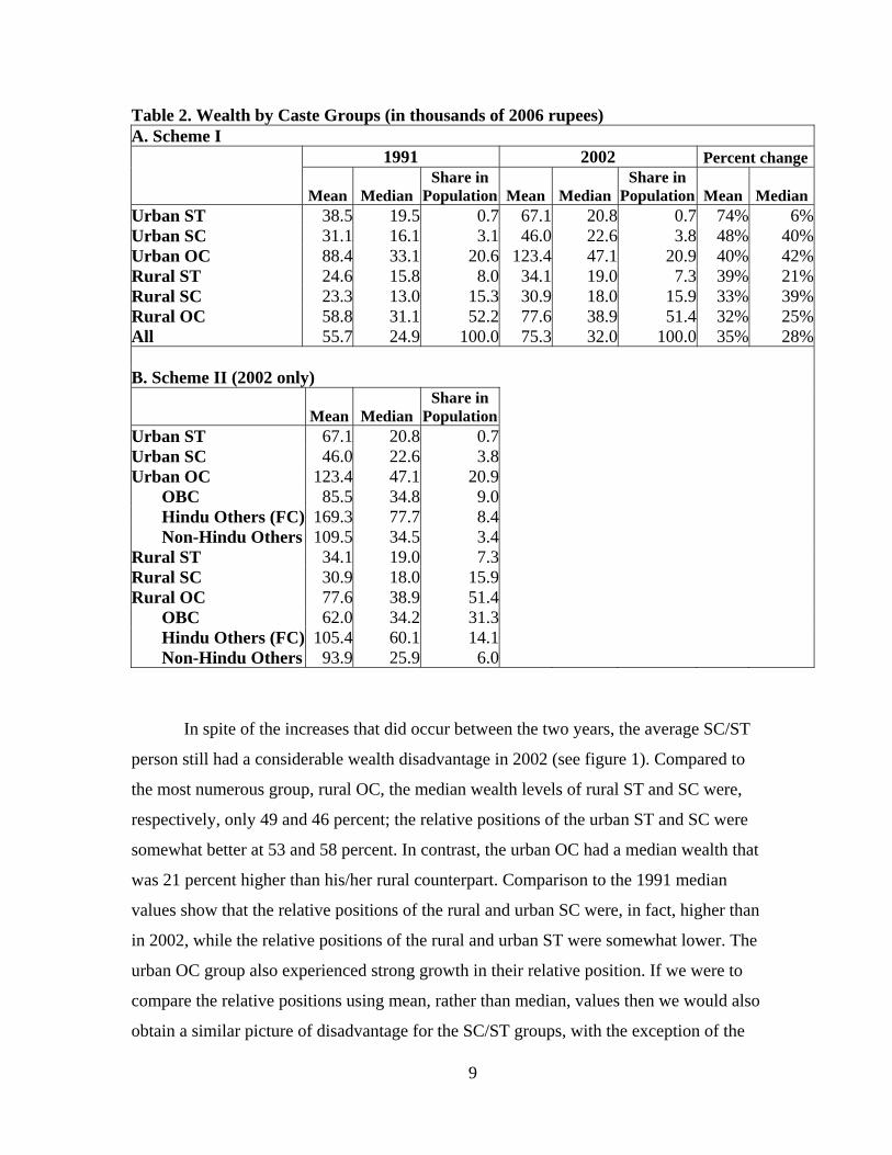
Table 2. Wealth by Caste Groups (in thousands of 2006 rupees) A. Scheme I 1991 2002 Percent change

Mean MedianShare in

Population Mean MedianShare in

Population Mean MedianUrban ST 38.5 19.5 0.7 67.1 20.8 0.7 74% 6%Urban SC 31.1 16.1 3.1 46.0 22.6 3.8 48% 40%Urban OC 88.4 33.1 20.6 123.4 47.1 20.9 40% 42%Rural ST 24.6 15.8 8.0 34.1 19.0 7.3 39% 21%Rural SC 23.3 13.0 15.3 30.9 18.0 15.9 33% 39%Rural OC 58.8 31.1 52.2 77.6 38.9 51.4 32% 25%All 55.7 24.9 100.0 75.3 32.0 100.0 35% 28% B. Scheme II (2002 only)

Mean MedianShare in

Population Urban ST 67.1 20.8 0.7 Urban SC 46.0 22.6 3.8 Urban OC 123.4 47.1 20.9

OBC 85.5 34.8 9.0 Hindu Others (FC) 169.3 77.7 8.4 Non-Hindu Others 109.5 34.5 3.4

Rural ST 34.1 19.0 7.3 Rural SC 30.9 18.0 15.9 Rural OC 77.6 38.9 51.4

OBC 62.0 34.2 31.3 Hindu Others (FC) 105.4 60.1 14.1 Non-Hindu Others 93.9 25.9 6.0

In spite of the increases that did occur between the two years, the average SC/ST

person still had a considerable wealth disadvantage in 2002 (see figure 1). Compared to

the most numerous group, rural OC, the median wealth levels of rural ST and SC were,

respectively, only 49 and 46 percent; the relative positions of the urban ST and SC were

somewhat better at 53 and 58 percent. In contrast, the urban OC had a median wealth that

was 21 percent higher than his/her rural counterpart. Comparison to the 1991 median

values show that the relative positions of the rural and urban SC were, in fact, higher than

in 2002, while the relative positions of the rural and urban ST were somewhat lower. The

urban OC group also experienced strong growth in their relative position. If we were to

compare the relative positions using mean, rather than median, values then we would also

obtain a similar picture of disadvantage for the SC/ST groups, with the exception of the

10

urban ST whose mean wealth is 86 percent of the mean wealth of the rural OC (as

compared to only 58 percent in terms of median wealth).

Figure 1. Disparity in Wealth by Caste, 1991 and 2002 (Ratio to Mean or Median Values of Rural OC)

As noted earlier, we are forced to treat the OC as a single category for comparing

the two years because the 1991–92 data does not allow for further breakdown of this

group along caste/religion lines. However, such a breakdown is possible in 2002–03 and

the structure of disparities among caste groups can be better seen in terms of what was

referred to earlier as Scheme II (panel B of table 1 and figure 2). Irrespective of their

urban or rural location, the average OBC person has an amount of wealth that was a little

less than 90 percent of the average rural OC person. The average person in the group

labeled “Non-Hindu Others” and living in an urban area has as much wealth as the

average OBC; those in the rural areas have significantly less, though more than that of the

average SC or ST person. The most advantaged subgroup in the OC group is the Hindu

forward castes (FC); the median wealth in the urban segment of this group is twice as

much as rural OC, while its rural segment has a median that was 54 percent higher than

rural OC.

0.00

0.20

0.40

0.60

0.80

1.00

1.20

1.40

1.60

1.80

Mean Median Mean Median

1991 2002

Rat

io

Urban STUrban SCUrban OCRural STRural SC

11

Figure 2. Disparity in Wealth among OC Groups, 2002 (Ratio to Mean or Median Values of Rural OC)

The ranking of the ten groups (in Scheme II) in terms of median wealth follows a

pattern that one might expect a priori: the Hindu forward castes are at the top (urban,

followed by rural). Immediately below them are the OBC groups and urban non-Hindu

others who have quite similar levels of median wealth. At the bottom, we have the most

disadvantaged (urban, followed by rural). The rural non-Hindu others occupy a place

immediately above the most disadvantaged and below everyone else.

If we were to use the mean values to rank the groups, the pattern shifts somewhat

(figure 2). The top group—urban, Hindu FC—still maintain their lead and the rural SCs

and STs held their status as the worst-off. Rural Hindu FC slip to the third place, with the

second place taken by the urban, non-Hindu others. Rural non-Hindu others occupy the

fourth place, followed by the urban OBC, urban ST, rural OBC, and then urban SC. The

reranking of the groups is an indication of the extent to which within-group inequalities

differ, a subject to which we return below.

Comparison of within-group distributions reveals that caste divisions and the

urban-rural divide act as distinct, yet interrelated, influences on the overall wealth

0.00

0.50

1.00

1.50

2.00

2.50

OBC HinduOthers

Non-HinduOthers

OBC HinduOthers

Non-HinduOthers

Rat

io MeanMedian

Urban Rural

12

distribution (see table 3). The differences between the distributions of the individual

groups are plotted on the vertical axis in figure 3 as ( ij ip p− ), which expresses the

deviation between the percentile cutoff of the jth group ( ijp ) from the overall percentile

cutoff ( ip ) at the ith percentile. Strikingly, only the Hindu FC stay in the positive territory

throughout the distribution, while the SC and ST groups stay in the negative territory

throughout the distribution. The cutoff values for the former became increasingly higher

than the overall values (most markedly for the urban, forward caste Hindus), while for the

latter they became increasingly lower as we move to higher echelons of the wealth

distribution. The other two groups, OBC and non-Hindu other, display more complex

patterns. Lower portions of the urban OBC and non-Hindu other distributions have cutoff

values that are below the cutoff values for the overall distribution, but the higher portions

have values that are higher, especially for the non-Hindu others. The rural segments of

these communities diverge from one another markedly. While the bottom 60 percent of

rural OBC enjoy higher than overall cutoff values, the top 40 percent in their distribution

have cutoff values that are increasingly lower. The opposite pattern can be observed for

the rural non-Hindu others.

13

Table 3. Percentile Cutoffs for Scheme II, 2002 (in thousands of 2006 Rs.) Percentile Urban

ST Urban

SC Urban OBC

Urban FC

Urban NH

Rural ST

Rural SC

Rural OBC

Rural FC

Rural NH All

5 0.8 0.7 1.1 2.5 1.0 2.7 2.1 3.4 6.1 2.4 2.410 1.8 2.0 3.1 6.0 2.1 4.8 4.0 6.6 12.0 4.5 5.115 3.3 3.7 5.8 11.0 4.7 6.3 5.5 9.5 18.1 5.9 7.620 5.2 5.6 8.8 17.3 8.3 7.7 7.0 12.3 22.8 7.3 10.225 7.0 7.9 12.3 24.5 11.2 9.3 8.6 15.2 27.7 9.5 12.930 9.8 10.6 16.1 33.1 14.5 11.0 10.1 18.3 33.0 11.8 16.035 12.0 13.4 20.1 42.2 18.0 12.6 11.9 21.6 39.2 14.8 19.340 14.7 16.3 24.2 52.8 22.8 14.7 13.6 25.6 45.5 17.9 23.045 18.2 19.4 29.0 64.6 27.9 16.6 15.8 29.7 52.5 21.4 27.350 20.8 22.6 34.8 77.7 34.5 19.0 18.0 34.2 60.1 25.9 32.055 23.6 27.2 41.4 93.1 42.0 21.6 20.3 39.1 68.9 31.0 37.660 28.9 31.0 49.0 111.7 52.1 24.7 23.3 45.0 78.9 38.1 44.465 38.0 35.1 58.4 131.7 65.3 28.5 26.6 51.3 89.9 46.8 52.370 49.0 41.1 70.5 155.5 84.5 32.0 31.0 60.1 104.2 59.0 62.875 61.4 50.4 83.9 191.8 107.7 37.3 36.2 70.8 122.4 76.7 76.380 77.3 63.6 106.9 235.0 139.1 43.8 43.2 83.9 145.3 104.1 94.585 102.9 81.8 143.2 290.9 189.9 52.8 52.2 102.8 181.2 145.1 122.290 144.9 109.8 192.3 379.3 273.9 71.6 66.5 136.1 230.5 220.8 170.195 220.6 168.8 313.1 562.9 429.0 110.4 98.3 205.9 331.0 402.3 272.3

Figure 3. Deviation from Overall Percentile Cutoffs by Caste at Selected Percentiles, 2002 (in thousands of 2006 Rs.)

-200-175-150-125-100-75-50-25

0255075

100125150175200225250275300325

5 10 15 20 25 30 35 40 45 50 55 60 65 70 75 80 85 90 95

Percentiles

Thou

sand

s of

Rs

Urban STUrban SCUrban OBCUrban FCUrban NHRural STRural SCRural OBCRural FCRural NH

14

The direction and amount of the urban-rural disparity within caste groups varies

across the distribution. This can be illustrated by defining the following statistic for group

j at percentile i :

,u rij ij

ij rij

p pg

p−

= (1)

where the urban-rural gap in wealth is expressed as a percentage of the percentile cutoffs

( p ) in the rural area for each caste group (the superscripts and u r represent,

respectively, the urban and rural areas).

Estimates of the urban-rural gaps are shown in figure 4 for selected percentiles,

with the bold horizontal reference line representing a situation of zero urban-rural

disparity. The wealth gap is in favor of rural individuals at the bottom of the distributions

of all castes. This is a reflection of the incidence of land ownership (however meager the

farm size might be) in the rural areas among the poor, in contrast to the greater presence

of propertyless individuals among the urban poor, irrespective of their caste identity.

Notable differences exist among the castes in the percentile point at which their

respective curves cross above the zero line. At one extreme are the non-Hindu others, for

whom the switch favoring the urban areas occurs at the 20th percentile; at the other

extreme, the switch occurs only at the 50th percentile for the OBC. The variation in the

amount of urban-rural disparity among the castes appears to be much smaller at any given

percentile point below the zero-line, i.e., when the disparity is in favor of the rural

individuals. Above the zero-line, when the disparity turns in favor of the urban persons,

the amount of disparity (at any given percentile point) among the castes appears to vary

much more. Clearly, the evidence suggests that the wealth advantage enjoyed by the

urban individuals within every caste becomes higher at the higher percentiles, with the

non-Hindu others standing out as a clear exception to this rule because the disparity in

favor of the urban individuals in this group declines after the 70th percentile. The urban

advantage skyrockets within the ST group in the top portions of the distributions, a result

consistent with the well-known fact that the rural tribal areas fall among the most

economically backward areas in India.

15

Figure 4. Urban-Rural Wealth Gap (as a Percent of Rural Wealth) by Caste at Selected Percentiles

We now revert to Scheme I in order to examine whether any significant

differences could be found among the groups in terms of the changes in wealth that

occurred between 1991 and 2002 across the entire distributions (figure 5). Urban ST is

the only group in which some of the percentile cutoffs in 2002 are roughly the same as, or

lower than, their 1991 levels. In contrast, the bottom half of the urban SC group generally

saw a much higher boost in their wealth levels than their counterparts in the other groups.

For the upper-middle portion (roughly from the 50th to 80th percentile), the urban OC

group experiences much faster growth than their counterparts in other groups. The

sharpest increases in wealth between 1991 and 2002 among the top 20 percent in all

groups occurs for the urban SC/ST groups. A negative correlation between the initial

amount of wealth and the subsequent gain could be found in the bottom half of the urban

SC and OC groups, as well as the rural ST and SC groups. In fact, the schedule for the

rural SC group slopes downward to the right almost throughout the distribution. Finally,

the rural OC group displays the most stable pattern: their schedule remained largely flat

for most of the distribution. The overall picture of changes across the distributions

-80%

-60%

-40%

-20%

0%

20%

40%

60%

80%

100%

120%

5 10 15 20 25 30 35 40 45 50 55 60 65 70 75 80 85 90 95

Percentile

Urb

an-R

ural

Gap ST

SCOBCFCNH

16

suggests a pattern of wealth accumulation that is not heavily biased in favor of those at

the top within each caste group, with the exception of the urban ST.

Figure 5. Percent Change in Wealth at Selected Percentiles by Caste Group, 1991 to 2002

-40%

-20%

0%

20%

40%

60%

80%

100%

5 10 15 20 25 30 35 40 45 50 55 60 65 70 75 80 85 90 95

Percentiles

Perc

ent

Urban STUrban SCUrban OCRural STRural SCRural OC

IV. DECOMPOSITION OF WEALTH INEQUALITY

A. Yitzhaki Decomposition

The picture of caste disparities in India sketched out so far can be made richer by relating

them to an analysis of overall wealth inequality. The tools of decomposition analysis

allow us to analyze the within-group and between-group disparities. Further, it would

allow us to develop summary measures that would express how demarcated in terms of

its wealth holdings a particular caste group is from another group or from the total

population. Also, comparisons of the degree of inequality among groups can be done.

The method of Gini decomposition developed originally by Shlomo Yitzhaki offers a

unified framework for addressing these issues.

17

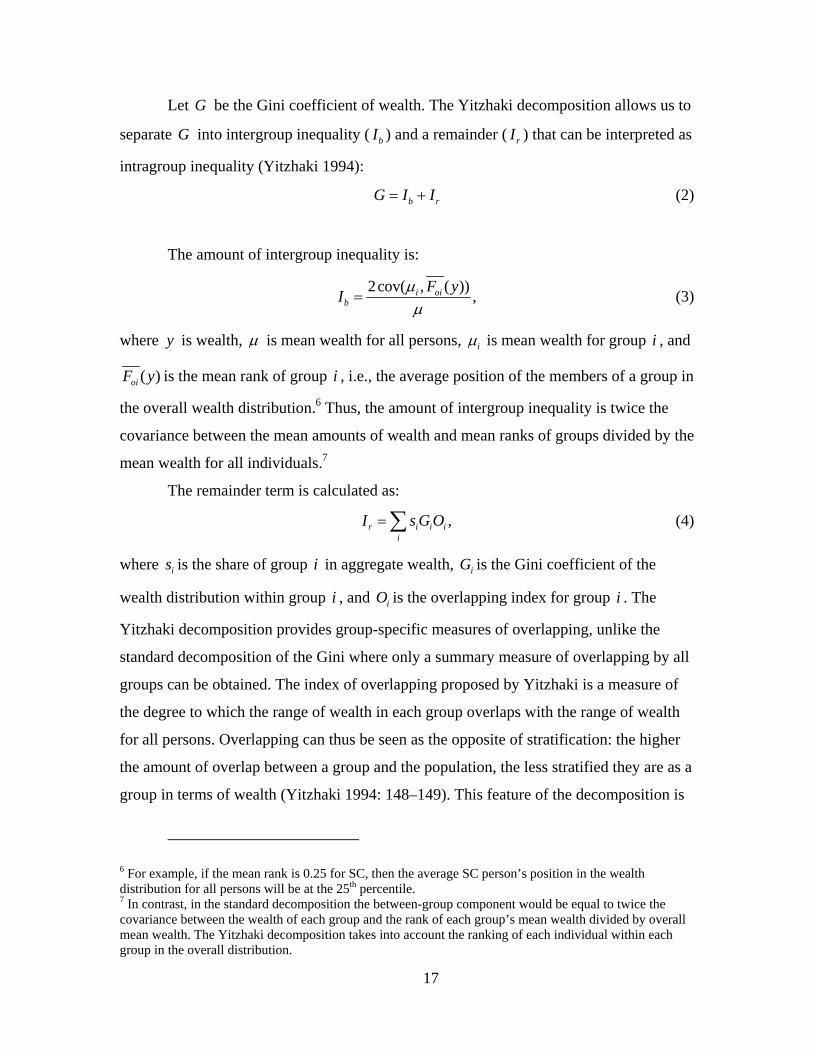
Let G be the Gini coefficient of wealth. The Yitzhaki decomposition allows us to

separate G into intergroup inequality ( bI ) and a remainder ( rI ) that can be interpreted as

intragroup inequality (Yitzhaki 1994):

b rG I I= + (2)

The amount of intergroup inequality is:

2cov( , ( )) ,i oib

F yI μμ

= (3)

where y is wealth, μ is mean wealth for all persons, iμ is mean wealth for group i , and

( )oiF y is the mean rank of group i , i.e., the average position of the members of a group in

the overall wealth distribution.6 Thus, the amount of intergroup inequality is twice the

covariance between the mean amounts of wealth and mean ranks of groups divided by the

mean wealth for all individuals.7

The remainder term is calculated as:

,r i i ii

I s G O=∑ (4)

where is is the share of group i in aggregate wealth, iG is the Gini coefficient of the

wealth distribution within group i , and iO is the overlapping index for group i . The

Yitzhaki decomposition provides group-specific measures of overlapping, unlike the

standard decomposition of the Gini where only a summary measure of overlapping by all

groups can be obtained. The index of overlapping proposed by Yitzhaki is a measure of

the degree to which the range of wealth in each group overlaps with the range of wealth

for all persons. Overlapping can thus be seen as the opposite of stratification: the higher

the amount of overlap between a group and the population, the less stratified they are as a

group in terms of wealth (Yitzhaki 1994: 148–149). This feature of the decomposition is

6 For example, if the mean rank is 0.25 for SC, then the average SC person’s position in the wealth distribution for all persons will be at the 25th percentile. 7 In contrast, in the standard decomposition the between-group component would be equal to twice the covariance between the wealth of each group and the rank of each group’s mean wealth divided by overall mean wealth. The Yitzhaki decomposition takes into account the ranking of each individual within each group in the overall distribution.

18

crucial for us since our objective is to ascertain the extent to which castes occupy or do

not occupy different segments of the wealth distribution.

The amount to which group i overlaps with the overall distribution is defined as:

cov ( , ( )) ,cov ( , ( ))

i oii

i i

y F yOy F y

= (5)

where ( )oiF y is the function that assigns to the members of group i their ranks in the

overall distribution, iF is the function that assigns to the members of group i their ranks

in the wealth distribution within that group, and covi indicates that the covariance is

according to the distribution within group i .8 The minimum value of iO is given by the

share of group i in the population and its maximum value is equal to 2. When the index

equals the minimum possible value, it suggests that the group in question is a perfect

stratum, i.e., it occupies an exclusive segment of the overall wealth distribution. If a

particular group has a range of wealth that coincides with the range of wealth of all

persons, then the index will be equal to 1. Finally, if the index is greater than 1, the

distribution of wealth within the group is much more polarized than in the overall

distribution. This can happen if the members of the group constitute two strata, one that

has higher and the other that has lower wealth than μ , the average wealth of all

individuals in all groups (Milanovic and Yitzhaki 2002: 162–163).

The index of overlapping defined in equation (4) is constructed from indexes that

indicate the amount by which a group overlaps with each of the other groups:

i i j jij i

O p p O≠

= +∑ (6)

\where ip is the share of group i in the total population and jiO is the index of

overlapping of group j by group i . Since the overlapping of a group by itself is equal to

1 by definition, its contribution to iO is equal to its relative size. The index of

overlapping of the overall distribution by a group is the weighted sum of overlapping of

8 In theory, the functions are actually cumulative distribution functions. However, when working with actual samples, the cumulative distribution function is estimated by the rank of the observation and, hence, our description of the functions as rank-assigning functions (Yitzhaki 1994: 149, n.1).

19

each of the other groups by that group, with the relative size of each group serving as the

weights.

In turn, the group-by-group overlapping indexes are calculated as:

cov ( , ( ))

,cov ( , ( ))

i jiji

i i

y F yO

y F y= (7)

where jiF is the function that assigns members of group i their ranks in the wealth

distribution of group j . The index jiO indicates the extent to which the wealth of

individuals in group j falls in the range of wealth of individuals in group i ; the higher

the fraction of group j that falls in the range of group i , the higher will be the value of

jiO . For a given fraction of group j that falls in the range of group i , the closer the

wealth of the individuals in that fraction are to the mean wealth of group i , the higher

will be the value of jiO . The index can take values between 0 (no overlap) and 2. Perfect

overlap occurs when the index equals 1, indicating that the rankings of members of group

i produced by iF and jiF are identical (Yitzhaki 1994: 150–152).

B. Within-Group vs. Between-Group Inequality

We now turn to the results of the Yitzhaki decomposition for our data.9 It is useful to

begin with the estimates of within-group and between-group caste inequality (table 4).

Overall wealth inequality shows very little change between 1991 and 2002. The share of

within-group and between-group inequality in overall inequality also remains roughly the

same between the two years. The within-group inequality (the rI term in equation [2])

accounts for the bulk of overall inequality in both years.

9 Decomposition of the Gini by groups was performed using the ANOGI module for STATA (version 9).

20

Table 4. Within- and Between-Group Inequality by Caste Gini points Percentage shares 2002 2002 1991 Scheme I Scheme II 1991 Scheme I Scheme II Overall Gini 0.648 0.655 0.655 100.0 100.0 100.0Within group 0.595 0.599 0.572 91.9 91.4 87.4Between group 0.053 0.056 0.083 8.1 8.6 12.6

The domination of the within term indicates there are other wide variations in the

characteristics of household members that are also expected to contribute to wealth

differentials within castes—occupation, age, education, industry of employment, and

number of earners in the household, to mention a few. Additionally, we would expect

product mix and fertility, among other things, to also have effects on the wealth of farmer

households. In 2002, we found that the share of within-group inequality is somewhat

lower (87 percent) under the more elaborate Scheme II (ten groups as compared to six in

Scheme I). Since the subgroups included in the OC group are themselves quite different

from each another in terms of their average wealth and distributions, the modest increase

in the share of between-group inequality under Scheme II is not out of line with our

expectations.

C. Within-Caste Inequality and Overlapping

The results from decomposing the remainder term along caste lines are shown in table 5.

Looking first at the column of overlapping indexes for caste groups under Scheme I

reveals that the urban ST and SC groups are hardly homogenous groups. Both have

values exceeding 1 for their overlapping indexes, indicating that there might be two

distinct strata, one quite rich and the other extremely poor, within each of these groups.

This is most striking in the case of the urban ST in 2002. The overlapping index for the

urban OC is almost 1 in 1991 and slightly lower in 2002, indicating the close similarity

between their distribution function and the distribution function for the entire population.

However, when these values are reckoned against their share in population (the minimum

value that can be taken by the overlapping index), they appear far more modest than the

urban SC/ST groups.

21

Table 5. Within-Group Inequality and Overlapping by Caste 1991 2002

Population

Share Wealth Share Gini Overlap Population

Share Wealth Share Gini Overlap

Urban ST 0.007 0.005 0.628 1.049 0.007 0.006 0.725 1.137Urban SC 0.031 0.017 0.627 1.056 0.038 0.023 0.632 1.051Urban OC 0.206 0.327 0.700 0.993 0.209 0.342 0.683 0.966

Urban OBC 0.090 0.102 0.677 1.016Urban FC 0.085 0.190 0.648 0.840Urban NH 0.034 0.050 0.713 1.054

Rural ST 0.080 0.035 0.526 0.913 0.073 0.033 0.568 0.969Rural SC 0.153 0.064 0.573 0.973 0.159 0.065 0.557 0.947Rural OC 0.522 0.551 0.595 0.918 0.514 0.530 0.609 0.929

Rural OBC 0.313 0.258 0.580 0.932Rural FC 0.141 0.197 0.563 0.791Rural NH 0.060 0.075 0.734 1.095

All 1 1 0.648 1 1 1 0.655 1

The rural groups in Scheme I have lower values for their overlapping indexes than

the urban groups, a result that is not surprising in light of the considerable rural-urban

wealth gaps that were discussed above (figure 4). Once again, when compared relative to

their shares in population, the rural OC group has a substantially lower degree of

overlapping than the rural SC/ST groups. Estimates for the subgroups included in OC in

2002 (Scheme II) show that the Hindu FC is the group with the lowest amount of

overlapping among all groups, while the non-Hindu other rural and urban groups take,

respectively, the second and third places in terms of overlapping (the urban ST was first,

as noted above). The higher degree of overlapping by the rural non-Hindu others as

compared to their urban counterparts is an exception to the pattern observed for the other

groups.

Within-caste inequality is the highest (above 0.670) among the urban ST, urban

non-Hindu others, and rural non-Hindu others, which, as we noted above, are also

characterized by overlapping indexes above 1. Excluding the latter, the other rural groups

all have a roughly similar amount of within-caste inequality (0.560 to 0.580). The urban

SC, OBC, and FC groups occupy an intermediate position (0.610 to 0.660) in within-

caste inequality. Comparisons against the 1991 values show that the only groups that saw

substantial change in wealth inequality are the ST groups, for whom there is a big

22

increase in inequality. This is especially true for the urban ST and is consistent with our

earlier finding about the big increases in the percentile cutoffs in the upper tail of the ST

wealth distribution (figure 5). Considered in conjunction with the jump in the overlapping

indexes, it appears that there is an emergence of a “nouveau rich” and growing income

polarization within the ST groups.

Apart from the index of overlapping for each group with the overall population,

the Yitzhaki decomposition also allows us to estimate pair-wise indexes of overlapping

among the groups (equation [7]). The estimates of the resulting overlapping matrix using

Scheme II for 2002 are shown in table 6 (panel A). The reference group (the caste

represented by the subscript i in the overlapping index jiO ) is shown in the rows of the

table; other groups are shown in the columns (the castes represented by the subscript j ).

Urban and rural FC groups have the highest degree of overlap with one another and a

much lower degree of overlap with all others. Thus, their status as the groups with the

lowest degree of overlapping with the population did not hold for the pair-wise

comparison. Overlapping of each of the other groups by the urban ST, SC, OBC, and the

non-Hindu others groups is generally high. In contrast, the overlapping of each of them

by the Hindu FC is much lower.

Table 6. Matrices of Overlapping and Ranks for Caste Groups, 2002

A. Overlapping

Urban ST

Urban SC

Urban OBC

Urban FC

Urban NH

Rural ST

Rural SC

Rural OBC

Rural FC

Rural NH

Urban ST 1 1.045 1.107 1.131 1.052 1.065 1.042 1.193 1.266 1.051Urban SC 0.938 1 1.009 0.928 0.933 1.051 1.032 1.119 1.111 0.963Urban OBC 0.881 0.916 1 1.062 0.951 0.905 0.885 1.068 1.179 0.928Urban FC 0.716 0.722 0.842 1 0.827 0.681 0.662 0.866 1.037 0.776Urban NH 0.915 0.944 1.041 1.133 1 0.928 0.906 1.100 1.230 0.970Rural ST 0.855 0.925 0.918 0.809 0.842 1 0.977 1.040 1.000 0.879Rural SC 0.852 0.924 0.889 0.739 0.812 1.021 1 1.017 0.934 0.868Rural OBC 0.794 0.849 0.908 0.903 0.838 0.851 0.831 1 1.070 0.826Rural FC 0.654 0.678 0.792 0.903 0.750 0.625 0.608 0.836 1 0.697Rural NH 0.937 0.973 1.075 1.163 1.029 0.971 0.945 1.148 1.277 1

23

B. Ranks

Urban ST

Urban SC

Urban OBC

Urban FC

Urban NH

Rural ST

Rural SC

Rural OBC

Rural FC

Rural NH

Urban ST 0.5 0.502 0.419 0.298 0.417 0.522 0.536 0.410 0.301 0.448Urban SC 0.498 0.5 0.410 0.282 0.409 0.526 0.541 0.402 0.283 0.445Urban OBC 0.581 0.590 0.5 0.362 0.492 0.622 0.634 0.502 0.381 0.531Urban FC 0.701 0.718 0.638 0.5 0.619 0.748 0.758 0.653 0.544 0.656Urban NH 0.582 0.590 0.508 0.381 0.5 0.616 0.628 0.509 0.400 0.534Rural ST 0.478 0.473 0.378 0.251 0.383 0.5 0.517 0.361 0.237 0.423Rural SC 0.463 0.459 0.366 0.242 0.371 0.483 0.5 0.348 0.227 0.409Rural OBC 0.590 0.598 0.497 0.347 0.491 0.639 0.652 0.5 0.363 0.538Rural FC 0.699 0.717 0.618 0.456 0.600 0.763 0.773 0.637 0.5 0.650Rural NH 0.551 0.555 0.469 0.344 0.466 0.576 0.591 0.461 0.350 0.5

The reason behind this apparent discrepancy can be understood by considering the

overlapping between the urban ST and urban FC. The overlapping of urban ST by urban

FC is only 0.716. This reflects the fact there are relatively few urban ST individuals in the

urban FC wealth range. Consequently, the ranks of urban FC individuals, when each of

them is placed in the wealth distribution of urban ST, did not differ much from each other

for a large number of them, thus reducing the size of the covariance in the numerator of

equation (7). On the other hand, the overlapping of urban FC by urban ST is much larger,

at 1.05, reflecting the fact that there are relatively more urban FC individuals in the urban

ST wealth range.

The overlapping of rural ST and SC by each of these groups is higher than the

overlapping of their urban counterparts by the same groups. For example, the overlapping

of rural ST by rural SC is 1.02, while the overlapping of urban SC by rural SC is lower, at

0.92. Further, the overlapping of rural OBC, FC, and NH groups by, respectively, the

rural SC and ST is higher than the overlapping of urban OBC, FC, and NH groups (e.g.,

the overlapping of rural FC by rural SC was 0.934, as against only 0.739 for urban FC).

This suggests that the distributions of rural ST and SC are more similar to each other than

to the members of their own community in the urban areas and that they have at least

some members with amounts of wealth that match the wealth of wealthier individuals

from the rural residents of other communities.

However, the rural-urban patterns of overlapping are quite different for the rural

OBC and FC groups. Their wealth distribution is more similar to the urban residents of

their own communities than to the SC or ST in the rural areas. For example, the

24

overlapping of rural SC by rural OBC is only 0.831, while the overlapping of urban OBC

by rural OBC is higher, at 0.908. Similarly, the overlapping of rural ST by rural FC is

quite low at 0.625 compared to the overlapping of urban FC by rural FC that stood at

0.903. The overlapping relation between the rural OBC and rural FC, as well as that

between the rural NH and rural FC, mirrors the relationship between urban ST and urban

FC that is discussed above.

The index of overlapping is sensitive to extreme values because it depends on the

ranks and amounts of wealth of individuals in each caste. Hence, an examination of the

ranking of one caste in terms of another is instructive. Such an exercise can answer the

following type of question: at what percentile of the forward caste wealth distribution is

an average SC person located? The average rank of each caste in the distribution of other

castes can be displayed in a matrix of ranks. Along the row labeled “Urban ST,” for

example, we can read off the average rank of an individual in that group in the wealth

distribution of each of the other groups. Since the ranks are normalized to lie between 0

and 1, the average rank of a group in its own distribution will be 0.5 (i.e., the 50th

percentile).

The matrix of ranks for caste groups under Scheme II is shown in table 6 (panel

B). Forward castes clearly dominate other groups in terms of this indicator, too. If we

look at the entries under the column labeled “Urban FC,” it is evident that the average

rank of all groups except rural FC is placed below the 40th percentile of the urban FC

wealth distribution; the rural FC’s average rank is at the 45th percentile. Similarly, the

entries in the “Rural FC” column are also below the 40th percentile for all groups except,

obviously, their urban counterparts.10 Viewed from another angle, this means that the

average ranks of all the other groups are at their lowest levels when they are placed in the

distribution of forward castes. The most numerous of the groups, the rural OBC, have a

mean rank above the 50th percentile in the distributions of all SC and ST groups and

close to the 50th percentile for the non-Hindu others and urban OBC distributions.

The average rural ST and SC ranks are below the 40th percentile in the

distributions of all other non-ST/SC groups, except for the non-Hindu others, where their

10 The sum of the average rank of group j’s rank in group i’s and the average rank of group i’s rank in group j’s distribution will be equal to 1.

25

ranks were at the 41–42nd percentile and slightly below the middle in the distributions of

their urban counterparts. Even though they have high values for their overlapping index,

the average urban ST and SC ranks are in the bottom half of the distribution of all other

groups, except that of their rural counterparts, where they are slightly above the middle.

Their ranking is the lowest (roughly at the 30th percentile) in the FC distributions,

somewhat higher (roughly at the 40th percentile) in the OBC distributions, and the

highest (roughly at the 45th percentile) in the NH distributions.

V. CONCLUSION

The average SC/ST person in India has a substantial disadvantage in wealth relative to

people from other groups in both years of analysis. Among these other groups, the FC

Hindus are the clear leaders in median wealth in both the rural and urban areas. For the

second survey year (2002–03), the OBCs and non-Hindus occupied positions that placed

them noticeably above the SC/ST groups, but significantly below the FC in terms of

median wealth values. In a worrisome trend, the relative median wealth of the rural and

urban ST is, in fact, lower in 2002 than in 1991. A similar picture of SC/ST disadvantage

and forward caste advantage is evident throughout the distributions in terms of gaps in

percentile cutoffs. Estimates of the matrix of ranks for caste groups also confirm the

existence of sizeable wealth gaps between the forward castes and everyone else.

Considered in conjunction with the findings documented in other studies regarding the

considerable shortfalls of the average SC/ST person in consumption, education, and

development indices, the picture that emerges is one of comprehensive and persistent

disadvantage for the disadvantaged groups in contemporary India.

Our decomposition analysis shows that inequality between castes (between-group

inequality) accounts for as much as 13 percent of overall wealth inequality in 2002. The

less elaborate caste schema (three instead of five) that we were forced to use for 1991 due

to data limitations results in a lower share of between-group inequality (8 percent). The

major determinant of between-group inequality is the large gap between SC/ST groups

(especially rural) and the forward castes (especially urban) in average wealth. It would be

interesting to compare this result to the results that arise from using other variables to

26

classify the population (e.g., age or education). However, it is reasonable to expect that

irrespective of the “grouping variable” used, the share of within-group inequality is likely

to be the dominant factor in overall inequality. There are, inevitably, other wide

variations in the characteristics of households that, when taken together, are likely to

contribute more than the classifying variable itself to wealth differentials within any

group.

Results from our decomposition analysis also indicate that the forward caste

Hindus have a fairly low degree of overlapping with the overall population and,

especially, with the SC/ST groups, i.e., they are more stratified in terms of their wealth

distribution. The other groups show a fairly high degree of overlapping with the overall

population, as well as with each other. Evidence of a polarized distribution could be

detected for four groups—urban ST, urban NH, rural NH, and urban SC (overlapping

index greater than 1). The first three of these groups have within-group inequality that is

much higher than the overall inequality, while the Gini coefficient for the last group was

lower than the overall Gini coefficient.

With the exception of the rural SC, the other three SC/ST caste groups—urban

ST, rural ST, and urban SC—witnessed increases in within-group inequality between

1991 and 2002. This was especially striking for the ST. Given its occurrence along with

the deterioration in the median wealth of the group compared to the rest of the

population, we might be witnessing the emergence of a “nouveau rich” or creamy layer

stratum and growing income polarization within the ST groups.

27

REFERENCES Barooah, Vani K. 2005. “Caste, Inequality and Poverty in India.” Review of Development

Economics 9(3): 399–414. Beteille, Andre. 2007. “Classes and Communities.” Economic and Political Weekly

42(11): 945–950. Chatterjee, Partha. 1993. The Nation and its Fragments: Colonial and Postcolonial

Histories. Princeton: Princeton University Press. Chaudhury, Pradipta. 2004. “The ‘Creamy Layer’: Political Economy of Reservations.”

Economic and Political Weekly 39(20): 1989–1991. Deshpande, Ashwini. 2000. “Recasting Economic Inequality.” Review of Social Economy

58(3): 382–399. ————. 2001. “Caste at Birth? Redefining Disparity in India.” Review of Development

Economics 5(1): 130–144. Dumont, Louis. 1970. Homo Hierarchicus: The Caste System and Its Implications

(Nature of Human Society). London and Chicago: George Weidenfeld and Nicholson Ltd. and University of Chicago.

Frick, Joachim R., Jan Goebel, Edna Schechtman, Gert G. Wagner, and Shlomo Yitzhaki.

2004. “Using Analysis of Gini (ANoGi) for Detecting Whether Two Sub-Samples Represent the Same Universe: The SOEP Experience.” Discussion Paper No. 1049. Bonn: The Institute for the Study of Labor (IZA).

Gupta, Dipankar. 2000. Interrogating Caste: Understanding Hierarchy and Difference in

Indian Society. New Delhi: Penguin Books. Hasan, Rana, and Aashish Mehta. 2006. “Under-representation of Disadvantaged Classes

in India.” Economic and Political Weekly 41(35): 3791–3796. Jayadev, Arjun, Sripad Motiram, and Vamsi Vakulabharanam. 2007. “Patterns of Wealth

Disparities in India During Liberalization.” Economic and Political Weekly 42(38): 3853–3863.

Kojima, Yoko. 2006. “Caste and Tribe Inequality: Evidence from India, 1983–1999.”

Economic Development and Cultural Change 54(2): 369–404. Mehrotra, Santosh. 2006. “Well-Being and Caste in Uttar Pradesh.” Economic and

Political Weekly 41(40): 4261–4271.

28

Milanovic, Branko, and Shlomo Yitzhaki. 2002. “Decomposing World Income Distribution: Does the World Have a Middle Class?” Review of Income and Wealth 48(2): 155–178.

Mohanty, Mritiunjoy. 2006. “Social Inequality, Labour Market Dynamics and

Reservation.” Economic and Political Weekly 41(46): 3777–3789. Munshi, Kaivan, and Mark Rosenzweig. 2006. “Traditional Institutions Meet the Modern

World: Caste, Gender, and Schooling Choice in a Globalizing Economy.” American Economic Review 96(4): 1225–1252.

National Sample Survey (NSS). 2005. “Household Assets and Liabilities in India (as on

30.06.2002).” Report, November. New Delhi: Government of India, Ministry of Statistics, National Sample Survey Organization.

Srinivas, M.N. 2000. Social Change in Modern India. India: Orient Longman. Srinivasan, K., and S.K. Mohanty. 2004. “Deprivation of Basic Amenities by Caste and

Religion.” Economic and Political Weekly 39(7): 728–735. Subramanian, S., and D. Jayaraj. 2006. “The Distribution of Household Wealth in India.”

Paper prepared for UNU-WIDER project meeting, May 4–6. Helsinki: World Institute for Development Economics Research (WIDER).

Sundaram, K. 2006. “On Backwardness and Fair Access to Higher Education in India:

Results from NSS 55th Round Surveys, 1999–2000.” Economic and Political Weekly 41(50): 5173–5182.

Yitzhaki, Shlomo. 1994. “Economic Distance and Overlapping Distributions.” Journal of

Econometrics 61(1): 147–159.