Embed Size (px)
Citation preview

ISSN No. 2454 – 1427
CDE June 2017
The Impact of MGNREGA on Agricultural Outcomes and the Rural Labour Market: A Matched DID Approach
Deepak Varshney, Deepti Goel and J.V. Meenakshi
Department of Economics, Delhi School of Economics,
University of Delhi
Working Paper No. 277 http://www.cdedse.org/pdf/work277.pdf
CENTRE FOR DEVELOPMENT ECONOMICS DELHI SCHOOL OF ECONOMICS
DELHI 110007
1
The Impact of MGNREGA on Agricultural Outcomes and the Rural
Labour Market: A Matched DID Approach
Deepak Varshney, Deepti Goel and J.V. Meenakshi
June 7, 2017
Abstract:
This paper attempts to address the impact of the MGNREGA on the rural agricultural sector, focusing on cropping patterns, irrigated area, crop yields, wages and rural employment. The analysis is based on two data sources: the first is a unique district-season level panel dataset that we construct using multiple sources; and the second is unit-record data from the NSS Employment Unemployment Surveys. To identify causal effects, we employ a difference-in-difference matching (DIDM) procedure, where districts are matched based on propensity scores; the use of propensity scores represents a novel aspect of this paper. We also examine pre-programme trends for each outcome variable to provide a check on the validity of our estimates. Our results indicate modest changes in cropping patterns that are state- and period-specific; however they do not indicate any improvements in crop yields that were expected given the MGNREGA’s focus on investments in irrigation, although there is some evidence that irrigated area may have expanded after a lag. We also find that there is no systematic evidence of impact on wages, and therefore no evidence that public works employment in MGNREGA crowded out casual labour in agriculture.
JEL classification codes: J31, J46, J48, Q15
Keywords: MGNREGA, Public Works, Agriculture
Ackowledgements: We thank Anirban Kar, Ashwini Deshpande, K.L.Krishna and Uday
Bhanu Sinha for useful comments. Any errors are ours.

2
The Impact of MGNREGA on Agricultural Outcomes and the Rural
Labour Market: A Matched DID Approach
1. Introduction
The Mahatma Gandhi National Rural Employment Guarantee Act (MGNREGA or the
‘Scheme’), enacted by the Indian parliament in September 2005, provides a legal guarantee of
100 days of employment to households willing to provide unskilled labour. It has, among its
objectives, “the creation of durable assets and strengthening the livelihood resource base of the
rural poor…” (GOI 2005). In particular, the Act has an explicit focus on water-related
infrastructure: Schedule I of the Act (GOI 2005) says, “The focus of the Scheme shall be on
the following works in order of their priority: (i) water conservation and water harvesting (ii)
drought proofing…(iii) irrigation canals including micro and minor irrigation works ….”
Another notable feature of the Act is the provision of an equal minimum wage to both men and
women.
Although a range of impacts of the MGNREGA have been documented in the literature,1 this
paper focuses on the extent to which the scheme has influenced agricultural outcomes, on
which the literature is more limited. This is motivated by concerns that MGNREGA is affecting
agriculture adversely by bidding up wages, and causing farmers to switch to less labour
intensive crops or to quit agriculture altogether (Rangarajan, Kaul and Seema 2011).2
There are two major pathways by which impacts in agriculture may be seen. The first is through
the infrastructure generated under MGNREGA. According to government data, more than 50
percent of the total expenditure on assets was spent on water-related works in 2010/11,3 and
1These include employment and wages (Azam 2012; Berg et al. 2015; Imbert and Papp 2015; Zimmermann 2015), incomes (Jha, Gaiha, and Pandey 2009), consumption (Ravi and Engler, 2015), welfare (Deininger and Liu 2013; Imbert and Papp 2015), women’s empowerment (Khera and Nayak 2009), education of children (Afridi, Mukhopadhaya, and Sahoo 2016), and child anthropometric outcomes (Uppal 2009). See also Bhatia et al. (2016) and Sukhtantar (2016) for an overview of research on MGNREGA.2Rangarajan, Kaul, and Seema (2011) find that between 1999/2000 and 2004/5 about 19 million people were added to the agricultural work force, while between 2004/5 and 2009/10 about 21 million people moved out of it. They also note a greater fall in share of agricultural employment in the total work force between 2004/5 and 2009/10 as compared to 1999/2000 to 2004/05.3Unless noted otherwise, these are all crop years, beginning in July and ending in June.

3
through 2011/12, more than 4 million such works had been created (MORD 2012).4
Conditional on the quality of assets, it is reasonable to expect that MGNREGA may have
improved the availability of water for irrigation. Improved irrigation facilities may mean that
farmers are able to cultivate a second crop in areas where second season crops were not
normally cultivated (CSE 2008). Additionally, even if gross area under irrigation did not
increase, increased water availability may have resulted in a shift from low to high water
intensive crops within the same season, or may have translated into higher yields for existing
crops. A direct impact of MGNREGA on agriculture may, therefore, be assessed by examining
changes in gross irrigated area, cropping patterns, and crop yields.5
The second pathway through which agriculture may be affected is through a change in
agricultural wages. Given that at the time the scheme was introduced agricultural wages were
lower than MGNREGA wage,6 and that MGNREGA is backed by a legal guarantee, the
bargaining power of hired labour may have increased after the scheme was implemented,
raising their reservation wage and thereby increasing wages in agriculture. Additionally, even
though the public works are meant to be carried out primarily in the off-peak agricultural season
(Imbert and Papp 2015), MGNREGA may directly compete with agricultural activities in the
peak season because of the inappropriate timing of the implementation of works under the
scheme, and may thus have led to an increase in agricultural wages. Any resultant increase in
agricultural wages7 may have consequences for cropping patterns and productivity. For
example, it may have shifted cropping patterns from high- to low-labour intensive crops, and
labour saving methods, if sub-optimal, may have lowered crop yields.
Thus our primary objective is to evaluate the net effect of both these MGNREGA-induced
pathways, by evaluating changes in gross irrigated area, wages in agriculture, cropping patterns
and crop yields. In particular, we examine whether farmers are shifting to crops with lower
4Calculated from Management Information System (MIS) data, collected from MGNREGA portal, Ministry of Rural Development, Government of India. Accessed on 15th May 2012, http://164.100.129.6/Netnrega/mpr_ht/nregampr_dmu.aspx?flag=1&page1=S&month=Latest&fin_year=2010-20115It would also be useful to look at the impact on volume of water for irrigation as this may be a mechanism via which yields are affected. However, we are unable to study this as, to the best of our knowledge, data on irrigation volumes is not available.6See Table 10 for figures on casual wage in agriculture. In 2004/5, before MGNREGA was instituted, these were much lower than the minimum wages guaranteed under the scheme.7It is also possible that the scheme may have led to mechanization, that could potentially lower agricultural wages, as noted in Bhargava (2014).
4
labour and/or higher water requirements, and also whether crop yields have changed as a
consequence of MGNREGA.
A second objective is to assess the scheme’s impact on employment/labour use and wages,
disaggregated by sector (rural agriculture and rural non-agriculture), by type of labour contract
(casual, regular/salaried, and self-employed),8 and by gender. Note that we do not undertake a
disaggregated study of wages by contract type and restrict our analysis to casual wages only.
This is because a priori we do not expect regular wages to be affected by the scheme as
MGNREGA offers unskilled work on a voluntary basis for at most 100 days a year.
As detailed in Section 2.2, much of the literature that has considered labour market outcomes
thus far has focused on the private sector as a whole, aggregating over agriculture and non-
agriculture, and also across contract types. A more detailed analysis focusing on agriculture,
and specifically on casual sector within agriculture, is warranted for several reasons. For
instance, as noted above, to the extent that the MGNREGA has led to changes in cropping
patterns, this has implications for agricultural labour demand. It is possible that by only looking
at aggregate outcomes in the private sector, any change specific to agriculture may not be
discerned due to counteracting exogenous changes in non-agriculture. Furthermore, unlike
labour use in non-agriculture, agricultural labour use by its very nature is seasonal and more
likely to benefit from the consumption smoothing opportunities offered by MGNREGA. Also,
since typically non-agricultural wages are higher than both agricultural and MGNREGA
wages,9 those working in the non-agricultural sector are less likely to offer themselves for
public works employment. For these reasons, it is reasonable to believe that MGNREGA might
have a greater impact on labour use and wages in agriculture, and only a limited impact on
these outcomes in non-agriculture. It is, therefore, important to study them separately. To the
extent that crops that need more water also have higher labour requirements, the net impact of
the MGNREGA on agricultural labour demand may be higher or lower, depending on whether
cropping patterns have changed to toward labour-saving crops as a consequence of higher
wages (if realized), or towards more water-intensive crops as a consequence of better irrigation
(if realized). Therefore, the net effect on labour use and on wages in agriculture is ambiguous
and depends upon the magnitude as well as the direction of change in cropping pattern.
8Casual wage labour are persons engaged in other farm or non-farm enterprises and getting in return wage according to the terms of the daily or periodic (but not regular) work contract (NSSO 2006).9Table 10 shows that in 2004/5, before the institution of MGNREGA, wages in non-agriculture were higher than those in agriculture.
5
Looking at different contract types within agriculture, casual labourers and those self-employed
(with petty businesses) are most likely to be impacted given the self-targeted nature of the
MGNREGA. Those who are in regular/salaried jobs, or those who have a large enough asset
base (for example, farmers with mid- to large-sized holdings who work on their own farms),
are unlikely to offer themselves for short-term employment offered under the scheme. Hence,
it is also important to distinguish between contract types.
MGNREGA is also likely to have a differentiated impact by gender. There are several reasons
to expect that the scheme may disproportionately increase the labour force participation by
women. First, compared to men, labour force participation rates for women are very low in
India.10 Further, the Act mandates that at least one-third of employment be accounted for by
women. It also provides for crèche facilities at each worksite so that women with younger
children can participate. Finally, women who are reluctant to travel outside their village in
search of employment because of social taboos can now find opportunities locally. Compared
to men, therefore, these features may draw in a larger proportion of women into the labour
market who were engaged in domestic duties or were otherwise not in the labour force.
Correspondingly, there may be a greater impact on female casual wage. We, therefore,
specifically focus on female labour use and female casual wage rates.
The conceptual framework and empirical strategy employed in this paper extends that set out
in Azam (2012) and Imbert and Papp (2015). Like this literature we also take advantage of
phased roll out of the MGNREGA: It was initially implemented in February 2006 in the poorest
200 districts (districts are administrative subdivisions of states), termed the `Phase I’ districts;
was then extended to another 130 `Phase II’ districts in April 2007; and in April 2008 it was
introduced in the remaining `Phase III’ districts as well.11 Thus, in 2004/5, MGNREGA had
not been implemented anywhere in the country, in 2007/8 it had been implemented only in the
Phase I and II districts, and in 2009/10 it had been rolled out in all districts, including in Phase
III districts.12
10In 2004/5, labour force participation rate for males in rural India was 545 persons per thousand persons, while the corresponding figure for females was 287 (NSSO 2006).11Some district boundaries were redrawn during this period, and new districts created. In February 2006, the total number of districts in the country was 612. This increased to 633 by April 2008. Care has been taken to account for these changes in the empirical analysis (see Appendix B for more detail).12Although implementation in Phase III districts was officially initiated in April 2008, as noted in Imbert and Papp (2015), effective employment creation is likely to have been weak in the initial months since implementation. Therefore, in the empirical analysis, Phase III districts are assumed to be immune to the scheme in the last three months of 2007/8.

6
Given this phase-wise roll out across vastly distinct geographies, we estimate two sets of
impacts. The first of these, termed as the impact on Phase I and II districts under partial
implementation, assesses the initial impact of MGNREGA on the Phase I and II districts at a
time when the scheme had yet to be rolled out in the Phase III districts. Partial implementation
impacts are estimated by looking at outcomes in 2004/5 and in 2007/8 for Phase I and II
districts, and comparing the change over this period relative to the change over the same period
in the Phase III districts. However, we go further than the existing literature to estimate a second
set of impacts which assesses whether the same effects, both in magnitude and direction, are
observed in the richer Phase III districts once these districts had also been covered under the
scheme. This is termed as the impact on Phase III districts under full implementation, and is
obtained by looking at outcomes in 2007/8 and in 2011/12 for Phase III districts, and comparing
the change over this period relative to the change over the same period in Phase I and II
districts. Phase I and II districts act as the control districts in this case, and unlike in the previous
set of impacts, the control districts had the scheme in the both comparison years. Differences,
if found, between the two sets of impacts, namely, Phase I and II under partial implementation
and Phase III under full implementation, may be attributed either to the differences in the socio-
economic conditions between Phase I and II districts and Phase III districts, or to the partial
versus full roll out of the scheme.
A second aspect that distinguishes our empirical strategy is that unlike the literature, we use
matching techniques to create appropriate counterfactuals before computing double-difference
estimates of impact. We thus employ a difference-in-difference matching (DIDM) procedure
to identify the causal effect of the scheme (Heckman, Ichimura, and Todd 1997). Matching
makes it more likely that the underlying assumption of identical changes over time between
treatment and control districts in the absence of the scheme holds good.
Thus, we extend the existing literature in two important ways. The first is our comprehensive
focus on agricultural outcomes—including area under irrigation, cropping patterns, crop yields,
as well as casual labour market outcomes within agriculture. Second, we estimate two different
sets of matched impacts, comparisons across which show whether geography and scale of
program implementation matter.
The rest of the paper is organized as follows. The second section provides a brief review of
literature. The third section describes the datasets used and presents a ranking of states
according to successful MGNREGA implementation. The fourth section details the empirical
7
strategy. The fifth section presents summary statistics followed by causal impact results for our
first set of outcome variables, namely, gross irrigated area, agricultural wages, cropping
patterns and crop yields, using a district level dataset. The sixth section does the same for our
second set of outcomes variables, namely, ten mutually exclusive and exhaustive employment
categories and casual wages, using an individual level dataset. The seventh section presents the
conclusions.
2. Review of Literature
We present the literature in two sub-sections. The first covers studies related to irrigation,
cropping patterns, and crop yields. Most studies in this sub-section use methods that do not
result in causal estimates. The second sub-section covers studies related to the impact on
employment and wages.
2.1. MGNREGA and Irrigation, Cropping Patterns and Crop Yields
Kareemulla et al. (2009) study six villages of Anantpur district in Andhra Pradesh. They find
that only about 25 percent of the ponds that were taken up under MGNREGA were being
utilized for irrigation, primarily because there was no provision of channeling water to the farm
plots. They note, however, that the investment in ponds was recharging ground water. The
Indian Institute of Forest Management (2010) studies four districts in Madhya Pradesh to find
that households perceived that there was a significant improvement in the availability of
irrigation water. Tiwari et al. (2011) study Chitradurga district of Karnataka and find that there
was a significant improvement in ground water level in three out of the six study villages after
the introduction of MGNREGA. A study by the Indian Institute of Science (2013) in 10 villages
each from Andhra Pradesh, Karnataka, Madhya Pradesh and Rajasthan compared groundwater
levels before and after MGNREGA and similarly found that levels had increased. Verma and
Shah (2012) examine the rate of return for irrigation assets constructed under MGNREGA in
Bihar, Gujarat, Rajasthan and Kerala for the year 2009/10. They use cost-benefit analysis for
140 best-performing MGNREGA related assets and find that that 80 per cent of the assets
created recovered their investment in the first year itself.
Studies that consider the impact of the MGNREGA on cropping patterns and crop yields are
relatively limited. Centre for Science and Environment (2008) examines the impact of
MGNREGA on irrigation and cropping patterns in a single district each of Orissa and Madhya
Pradesh and finds that respondents in Madhya Pradesh perceived there to be an improvement

8
in irrigation availability, and a change in cropping pattern as a result, but respondents in Orissa
did not report any change. Aggarwal, Gupta, and Kumar (2012) study the implications of
eleven wells constructed under MGNREGA in a gram panchayat of Ranchi district in
Jharkhand on cultivation costs and profits. They find that there was a considerable
diversification of cropping patterns, especially toward vegetables, after the construction of the
wells, and that as a result farm profits in the command area of these wells increased from
Rs.7,635 per year to Rs. 15,728 per year.
Nearly all the studies reviewed above are associative in nature, in that they do not account for
possible biases in impact estimates resulting from endogeneity in participation. Studies that
explicitly estimate causal impacts include Gehrke (2014) and Bhargava (2014). Gehrke (2014)
examines the role of the MGNREGA in mitigating household’s uncertainty vis-à-vis income
streams and thereby affecting crop choices. Using data for Andhra Pradesh, she finds that
farmers have switched to more profitable but risky crops as a result of MGNREGA. Bhargava
(2014) examines the impact of MGNREGA on demand for agricultural technology. Using
agricultural census data he finds that the MGNREGA caused a 20 percentage point shift away
from labour-intensive technologies towards labour-saving technologies, particularly for small
farmers.
Our study contributes to the literature examining agricultural outcomes by providing the first
rigorous estimates for the causal impact on irrigated area at the all-India level, and for cropping
patterns and crop yields for three major states.
2.2. MGNREGA and Employment and Wages
Azam (2012) was the first to exploit the phase-wise roll out of the MGNREGA and use a
difference-in-difference (DID) approach to identify causal impacts of MGNREGA on
employment and wages. Using Employment Unemployment Surveys (the same dataset as we
use) for 2004/5 and 2007/8, he finds a positive impact on public works employment and on
labour-force participation rates, largely driven by changes in women’s employment. For the
same period, and following largely the same methodology, Imbert and Papp (2015) examine
the impact of the scheme on the composition of employment between public and private works,
disaggregated by season. They find a 1.2 percentage points increase in the fraction of days
spent in public works during the dry season (roughly corresponding to the agricultural off-peak
season), and a decline of 1.3 percentage points in private work in the same season. They
9
interpret this as evidence to suggest that private sector employment is being substituted by
employment in public works. Similarly, based on a panel survey of 3725-households conducted
by the World Bank in Andhra Pradesh in 2004, 2006, and 2008, Sheahan et al. (2016) also use
a difference-in-difference estimation strategy to conclude that the number of days in paid non-
MGNREGA employment has declined significantly in the state of Andhra Pradesh as a
consequence of the scheme. Zimmermann (2015) also uses EUS data but adopts a regression
discontinuity approach using data only for the year 2007/8. In contrast to the first two papers
mentioned above she finds that the MGNREGA did not impact employment in public works.
Thus, the evidence on the impact of MGNREGA on employment is mixed; this is also true of
the impact on casual wages. Both Azam (2012) and Imbert and Papp (2015) find a positive
impact with the latter finding a 4.7 percent increase in the dry season, and no change in the
rainy season (corresponding to the agricultural peak season). Similarly, Berg et al. (2015) use
a different data set—monthly data from Agricultural Wages in India (AWI) reports for the
period 2000 to 2011—but employ the same identification strategy to conclude that the scheme
resulted in a 4.3 percent increase in casual wages. In contrast to these papers, Mahajan (2014)
and Zimmermann (2015) find no impact on casual wages. Mahajan (2014) uses the same data
and the same methodology as adopted by Azam (2012) and Imbert and Papp (2015), but she
includes interactions between state and time dummies to capture state-specific time trends
which seem to explain away the positive results found in earlier papers.
Furthermore, the gender disaggregated impact is quite contrasting in these papers: While Azam
(2012) finds the positive impact on casual wage to be driven by female workers, Imbert and
Papp (2015) find it to be driven by male (and not female) workers and Berg et. al. (2015) find
the impact to be gender neutral.
We contribute to the literature examining labour market outcomes in the following ways. First,
as noted earlier, while studies such as the one by Imbert and Papp (2015) consider private and
public employment separately, they do not further disaggregate the private sector into
agriculture and non-agriculture. Also, they do not examine casual labour employment
separately, as we do in this paper. Second, for identifying causal estimates we use matching
before difference in differences which makes the assumption of identical time trends between
control and treatment districts more plausible. Finally, in addition to partial implementation
estimates, we also present full implementation estimates for the period 2007/8 to 2011/12.

10
3. Datasets and Ranking of States
To evaluate changes in gross irrigated area, agricultural wages, cropping patterns and crop
yields, we constructed a district-level panel dataset for the years 2000/1 through 2009/10. The
dataset, which we shall refer to as the crop-wage dataset, was collated from a large number of
sources, not all of which are readily available in the public domain (see Appendix A for details).
While it is meaningful to undertake the analysis of gross irrigated area and agricultural wages
at the all-India level, in order to study changes in cropping patterns and crop yields it is
important to consider a geography that is characterised by homogenous agro-climatic
conditions (to be able to identify competing crops), and at the same time is large enough to
have sufficiently large number of treatment and control districts. We consider state-season to
be such an appropriate geography and the analysis of cropping patterns and yields is confined
to the top three states in terms of MGNREGA implementation.
For our second objective, which is to examine changes in employment and casual wages in
rural India, we use repeated cross-sections of individual level data from Employment-
Unemployment Surveys (EUS) conducted by the National Sample Survey Organization. The
surveys used correspond to the years 1999/2000, 2004/5, 2007/8 and 2011/2 and are
representative at the national and state levels. To maintain comparability with other papers (in
particular with Imbert and Papp 2015), we consider individuals between 18 and 60 years of
age, living in rural areas of the 19 major states listed in Table 1.13 Construction and definitions
of the main outcome variables for both the datasets are presented in Appendix A.
We note two things. First, we study wages using two different datasets. Data on agricultural
wages from the crop-wage dataset does not distinguish between contract types; it is the average
wage paid to unskilled labour employed in agriculture. On the other hand casual wage in
agriculture from the EUS is restricted to wages paid to persons according to an ad hoc work
contract and excludes wages paid on a regular basis. Second, we have used two different, but
related, characterisations of seasons within an agricultural year. When discussing impacts on
cropping patterns and crop yields, we talk about seasons as kharif and rabi. Although the exact
months comprising these seasons vary by state, and by crop, in most parts of India sowing for
the kharif crops begins in July and harvesting is done by October or November, while sowing
13These states together cover 97 percent of the country’s rural population in 2004/5.

11
for the rabi crops begins in mid-November and harvesting is completed by April or May. When
discussing impacts on employment and wages we refer to seasons as dry and rainy.14 The dry
season refers to the months from January through June, while the rainy season from July
through December. The rainy season roughly corresponds to the agricultural peak season
because in most states it includes the sowing and harvesting of kharif crops, and the sowing of
rabi crops, all of which are highly labour intensive. On the other hand, the dry season may be
considered as the agricultural off-peak season as the only labour intensive operation during this
period is the harvesting of rabi crops.
3.1 Ranking of States according to MGNREGA Implementation
Dutta et al. (2012), and Liu and Barrett (2013), find substantial inter-state variation in the
implementation of MGNREGA with the latter finding that the scheme achieved effective
targeting in only about half of the Indian states. In the light of this, it is likely that the effects
of the MGNREGA are more pronounced—and therefore more readily apparent—when we
focus on only the states that have more successfully implemented the scheme. For this reason,
in addition to studying the impacts at the national level, we separately study the top three states
in terms of MGNREGA implementation.
Table 1 presents the ranking of all 19 states according to MGNREGA implementation. The
ranking is based on an index defined as the product of the scheme’s intensity and its coverage.
Intensity is the average, over participating households, of the number of days of MGNREGA
employment in a year. Coverage is the share of rural households that obtained (any)
MGNREGA employment. The final index for a state is the product of intensity and coverage,
each calculated as the average over the two years, 2008/9 and 2009/10. According to this
ranking, the top three performing states are Rajasthan, Andhra Pradesh, and Madhya Pradesh,
having average intensity figures of 72, 61 and 55, and average coverage rates of 79, 56 and 60
percent, respectively.15
4. Empirical Strategy
As stated in the introduction we exploit the phase-wise roll out of MGNREGA that facilitates
the application of DID. This strategy has been used by several papers including Azam 2012;
Berg et al. 2015, and Imbert and Papp 2015. However, as noted in Zimmermann (2015) and
14We change terminology to be consistent with other literature, in particular with Imbert and Papp 2015. 15Overall, our ranking compares well with that of Dutta et al. (2012).
12
Gupta (2006), although the scheme was meant to be implemented in poorer districts first, there
was significant deviation in the final selection of districts for early implementation. Keeping
this in mind, we deviate from the literature that has used DID to study the scheme’s causal
effects and adopt DIDM procedure instead.16
We implement the DIDM procedure in the following steps. First, using 2004/05 data, we match
each Phase I and II district with a weighted combination of Phase III districts such that the
predicted probability of receiving the scheme by 2007/08 is similar in both. We then compare
the outcomes in each Phase I and II district with the weighted average of outcomes across
matched Phase III districts. Implementing the matching procedure essentially involves
modifying the individual level survey weights provided by the NSSO. This is explained in
Appendix B.
The DIDM framework allows us to identify the impact under the maintained hypothesis that,
conditional on covariates, there would have been no difference in time trends between Phase I
and II and Phase III districts in the absence of the scheme. As noted earlier, even before
MGNREGA was implemented, the two sets of districts differed in their socio-economic
characteristics. Implementation of propensity score matching reduces the concern that the
maintained hypothesis may not hold good. Appendix Table C1 confirms this: In 2004/5,
without matching, compared to Phase III districts, Phase I and II districts have a larger share
of SC/ST households, less educated individuals, lower consumption expenditure per
household, lower agricultural wages, and lower cultivable land per household. After matching,
these differences disappear. To be completely certain that we are indeed capturing the effects
of MGNREGA, we also examine pre-program changes in each outcome over the period
1999/2000 to 2004/5, and give causal interpretations only when there is no difference in pre-
program changes between treatment and control districts.
Next we present the regressions used to estimate the impact under partial implementation,
followed by that under full implementation. We present the empirical specifications in the
context of regressions run using EUS data. Similar specifications, with minor modifications,
were used when using the crop-wage data.
16We restrict ourselves to a standard DID for the analyses of cropping pattern and crop yields as these are done at the state-season level and the number of districts is not large enough to implement matching sensibly, e.g. Andhra Pradesh has only 22 districts.

13
4.1. Impact on Phase I and II districts under Partial Implementation
The DIDM estimate on Phase I and II districts under partial implementation is given by the
following equation:
= + ( 07 1&2 ) + (,…, 07 ) + + + { } + (1 )
where i stands for individual, d for district, s for Agro-Ecological Zone (AEZ) and t for year.
In the specification for partial implementation, t is either 2004/5 or 2007/8.
When studying outcomes from the EUS, Y is one of the following:
(a) Time share in one of ten employment categories listed in section A2 of Appendix A. For
each category, Y is a value between 0 and 1, and captures the fraction of time spent in that
category during the reference week.17
(b) Logarithm of casual wage in agriculture (and separately in non-agriculture).
When using the crop-wage dataset, Y is one of the following:18
(a) Logarithm of share of gross irrigated area in total cropped area.
(b) Logarithm of agricultural wage.
(c) Share of crop acreage in total cropped area.19
(d) Logarithm of crop yield.
The right hand side variables are as follows:
(a) T07 is a dummy variable for the year 2007/8.
(b) Phase1&2 is a dummy variable for whether the district is a Phase I or a Phase II district.
(c) {AEZk} is a set of dummy variables, one for each of the five AEZs in India: Coastal, Arid,
Hills, Irrigated, and Rain fed (Saxena, Pal, and Joshi 2001). The interaction between year and
zone dummies allows for AEZ specific time trends.20
17For example, if in the reference week of 7 days, a person spends 4.5 days as casual labour in agriculture and 2.5 days in domestic work, then Y takes values 0.64 and 0.36 for these two categories, respectively, and it takes the value 0 for all other categories. Note that this outcome variable is not in logarithms as for a given individual many categories take the value 0. 18In specifications for the crop-wage dataset, the subscript i is not applicable as the unit of observation is a district and not an individual.19Again, this variable is not in logarithms because even within a state-season strata, there are several districts which do not grow a particular major crop and therefore have 0 values for those crops. 20For the two outcomes analysed at the state-season level, namely, share of crop acreage in total cropped area and crop yield, AEZs are replaced by Agro-Ecological Zone Production Systems (AEZPSs). Each AEZPS is a

14
(d) X stands for individual covariates included to increase precision.21 These are: age; age
squared; marital status (never married, currently married, and residual other category); caste
(SC, ST, Other Backward Classes (OBC), and residual other category); Muslim; and education
(illiterate, primary and below, middle, secondary and above).
(e) Z stands for rainfall22 at the district level.23
(f) μ is a set of district fixed effects and
(g) is the error term.
is the DIDM impact estimator for Phase I and II districts under partial implementation when
equation (1) is run on the common support region with modified individual level matching
weights. Robust standard errors, clustered at the district-year level, have been used in this and
all other specifications mentioned in this section.
4.2 Impact on Phase III Districts under Full Implementation
The impact on Phase III districts under full implementation is given by the following equation:
= + ( 11 3 ) + (,…, 11 ) + + + { } + (2)
where the subscripts are as defined in equation (1). In this specification, t is either 2007/8 or
2011/2. T11 is a dummy variable for the year 2011/12, and Phase3 is a dummy variable for
Phase III districts. All other variables are defined similarly as in equation (1). is the DIDM
impact estimator for Phase III districts under full implementation.
Another issue is that intensity of implementation of the scheme in Phase I and II districts could
itself vary in moving from 2007/8 to 2011/12. This would also confound the effect of the
scheme on Phase III districts under full implementation. We find that this is not the case: for
the top 3 states in Phase I and II, 1.7 percent of time was spent in public works in 2007/8 and
homogenous group of districts with similar cropping pattern that falls within a single AEZ (Saxena, Pal, and Joshi 2001).21For specifications using the crop-wage dataset, the covariates are shares of: SC/STs, illiterates, currently married, Muslims and average age and age squared, all at the district level.22Monthly rainfall at the district level for the period from 1999/2000 to 2007/8 was obtained from International Crop Research Institute for Semi-Arid Tropics, ICRISAT, Hyderabad, and for the remaining years from IndianMeteorological Department, Government of India. 23For the agricultural wage outcome in the crop-wage dataset, Z also includes the proportion of SC/ST population and the literacy rate, both at the district level.
15
1.9 percent in 2011/12. For all India, the corresponding figures are 1.0 percent in 2007/8 and
1.3 percent in 2011/12.
5. Impact on Gross Irrigated Area, Agricultural Wages, Cropping Patterns and Crop Yields using Crop-wage dataset
Before we present the impact estimates we discuss some summary statistics.
5.1. Summary Statistics
Table 2 presents the average share of gross irrigated area in total cropped area. As expected,
in 2004/5, the average share of gross irrigated area in Phase I and II districts is lower than that
in Phase III districts by 10 percentage points. This difference is maintained in subsequent years
as well and continues to persist in 2009/10 even when the scheme was fully implemented in
the country.
Turning to real agricultural wages, in Table 3 we see that agricultural wages in Phase I and II
districts were lower than those in Phase III districts, in all three years: This is true for both men
and women, and in both the dry and the rainy seasons: the difference ranges from 7 to 9 rupees
per day for women and from 14 to 20 rupees per day for men (in 2004/5 prices).24
Table 4 presents the seasonal cropping patterns (crop shares in total cropped area) for each of
the top three states, separately for Phase I and II and for Phase III districts. Within a state-
season, we restrict ourselves to studying the set of at most five crops with the largest crop
acreages that together cover at least 90 percent of total cropped area between 2000/1 and
2005/6. Crops shares in Phase I and II districts are similar to those in Phase III districts in
Rajasthan, but are somewhat different in Andhra Pradesh and Madhya Pradesh. This raises
some concerns about whether cropping patterns are comparable across the two sets of districts
in these two states.
Table 5 presents similar summary statistics for crop yields, which indicate that, as expected,
crop yields are typically lower (or statistically no different) in Phase I and II districts compared
to Phase III districts.
24 Note that generating a balanced panel across all three years would have resulted in a loss of several observations and for this reason, the sample sizes are smaller for 2004/5. This means that impact estimates computed later in Table 7 for impact under partial implementation are based on a smaller sample size than those for full implementation; the estimation sample under each is however a balanced panel.

16
5.2. Impact on Gross Irrigated Area
Table 6 presents the DIDM impact estimates for the share of gross irrigated area in total
cropped area.25 We do not find differences in pre-program changes between 2000/1 and 2004/5
in the share of gross irrigated area between the two sets of matched districts which raises the
credibility of our estimates.
At the all-India level and for the top three states, we find an adverse impact of MGNREGA on
share of gross irrigated area with impact magnitudes being larger for the top three states. For
the top three states under partial implementation, we find that because of the scheme the share
of gross irrigated area grew at a rate that was 16 percentage points (p.p.) lower in Phase I and
II (i.e. treated) districts between 2004/5 and 2007/8. Under full implementation also, we find
that MGNREGA resulted in a smaller growth (lower by 17 p.p.) in the share of gross irrigated
area in Phase III districts between 2007/8 and 2009/10. Thus, in spite of the scheme’s focus on
water works, it did not manifest as an increase in gross irrigated area. These results are contrary
to expectation. A plausible explanation for the results under full implementation, is that the
effect of MGNREGA on gross irrigated area appears with a lag. In other words, water works
implemented under the scheme are ineffective in increasing gross irrigated area initially, but
improvements to existing infrastructure make these investments effective in raising gross
irrigated area subsequently. For example, Kareemulla et al. (2009) report in their study that
although ponds and water reservoirs got built, the connecting channels to plots of land were
only constructed later on. If this is indeed the case, then from 2007/8 to 2009/10, when
MGNREGA is being implemented for the first time in Phase III districts and is continuing in
Phase I and II districts, the scheme would result in higher growth in gross irrigated area in
Phase I and II districts relative to Phase III districts. None of these results preclude the
possibility that MGNREGA may have improved the volume of water available for irrigation.
5.3. Impact on Agricultural Wages
Table 7 presents the DIDM estimates of impact on real agricultural wages, disaggregated by
gender and by season. As in the case of gross irrigated area we did not find differences in pre-
program changes between the two sets of matched districts.
25In this discussion, we sometimes refer to share of gross irrigated area in total cropped area as simply the share of gross irrigated area.

17
At the all-India level, we do not find evidence that male agricultural wages were affected by
the scheme. In the top three states under partial implementation in Phase I and II districts, in
the dry (off-peak) season, there was no impact of the MGNREGA on male agricultural wages,
and it is only in the rainy (peak) season that there is weak evidence (at the 10 percent level of
significance) of an increase in agricultural wages for men. Wages for women in the rainy
season under partial implementation did increase—the evidence is stronger for the top 3 states
than for all-India. There does not have been any impact under full implementation in Phase III
districts.
5.4. Impact on Cropping Patterns
Table 8 presents the DID impact estimates for cropping patterns in each of the top three states,
separately for kharif and rabi seasons. We do not carry out the matching exercise for impacts
on crop shares and crop yields as the number of districts is too small. We italicize impact
estimates for outcomes with pre-program trends; these estimates cannot be interpreted to be
causal.
In the following paragraphs, we discuss the impacts for each state separately, first for the kharif
season and then for the rabi season. As mentioned earlier, the kharif season roughly coincides
with the rainy season, while the rabi season with the dry season.
Rajasthan: Looking at the top five crops grown in the state in the kharif season, one expected
a shift to lower labour intensive crops if one takes into account that for Phase I and II districts
under partial implementation there was a positive impact on agricultural wages in the rainy
season, but not on gross irrigated area. However, we do not find evidence for this. For Phase
III districts under full implementation, MGNREGA led to a greater increase in soyabean
acreage in Phase III districts compared to Phase I and II districts: there is a 2.6 p.p. greater
increase in jowar cultivation between 2007/8 and 2009/10. As indicated in Appendix Table C2,
jowar has lower labour and about the same water requirements relative to maize, although other
competing crops have still lower labour requirements. Thus, this increase in jowar acreage is
consistent with an increase in male wages in the rainy season under full implementation (this
impact on males wages is significant only at the 10 percent level of significance). In the rabi
season, under partial implementation, MGNREGA adversely affected wheat: Between 2004/5
and 2007/8, the scheme resulted in a 11.7 p.p. lower increase in wheat area share. As indicated
in Appendix Table C2, wheat is more labour intensive than other competing crops. We

18
conjecture that crop acreage under wheat may have been adversely impacted in Phase I and II
districts not directly by an increase in the agricultural wage rates in the dry season (as there
was no positive impact on agricultural wages in the top three states in this season), but that the
announcement of the MGNREGA and the subsequent increase in agricultural wages in the
kharif season translated into an expectation of similar increases in the rabi season and thus
altered crop choices. For Phase III districts under full implementation, MGNREGA resulted in
a 7.6 p.p. increase in crop acreage of wheat in Phase III districts relative to Phase I and II
districts. Since wheat has higher labour and water requirements compared to most competing
crops, this result is clearly not consistent either with the increase in female wages nor with the
lower rate of growth in irrigated area in these districts. It is possible that irrigated area is not a
good measure of the impact of the MGNREGA, as it may have improved water availability
more than irrigated area; however we do not have information on the volume of water. Further,
as seen later, there was no impact on wheat yields, which should have increased with improved
water availability.
Andhra Pradesh: In the kharif season, we find a positive impact on arhar acreage under partial
implementation. As indicated in Appendix Table C2, arhar requires least amount of labour
among other competing crops. This result may therefore be explained by an increase in
agricultural wages in the rainy season. Among rabi crops, under partial implementation, we
find a decline in paddy acreage (21.5 p.p.) accompanied by an increase in urad (15.6 p.p.) in
Phase I and II districts.26 Nagaraj et al. (2016) find a decline in labour use as a consequence of
MGNREGA in semi-arid villages of Telangana and Maharashtra. As indicated in Appendix
Table C2 that paddy is a very high labour and water intensive crop among competing crops.
This result may therefore be explained through a farmer’s expectation of wage rise in the dry
season after they saw an increase in agricultural wages in rainy season. Under full
implementation, we find an increase in acreage of gram. As indicated in Appendix Table C2,
gram requires less labour and water among competing crops. Once again, we conjecture that
this may have operated through an expectation of increased wages in the rabi season (because
of the experience in the kharif season) that did not, in the event, materialize.
26Bhaskar (2012) finds a decline in paddy cultivation but he finds switch towards cotton, but here we find switch towards urad.

19
Madhya Pradesh: For the five kharif crops, there is no evidence of MGNREGA affecting crop
shares under partial implementation. Under full implementation, we find an increase in jowar
acreage in Phase III districts relative to Phase I and II districts. As seen from the Appendix
Table C2, jowar is more water- and labour-intensive as compared to soyabean which is the
main crop in Madhya Pradesh. Once again, this is contrary to expectations given the increased
wages for men (significant at the 10 percent level) and lower increase in irrigated area in Phase
III districts relative to Phase I districts under full implementation. There is no evidence of
impact on rabi cropping patterns, neither under full, nor partial implementation.
Thus from a food security point of view, with the main crops, there is evidence that although
the MGNREGA adversely affected wheat area in Rajasthan initially it subsequently increased
under full implementation in Phase III districts. This represents a switch initially towards less
labour-intensive and later to more water-intensive crops and cannot be explained fully
through the two channels since the rate of increase in irrigated area in Phase III districts was
lower than in Phase I and II districts. There is evidence of a switch away from paddy to urad
in Andhra Pradesh, which is consistent with expectations.
5.5. Impact on Crop Yields
Table 9 presents the DID impact estimates for crop yields in each of the top three states,
separately for kharif and rabi seasons. The crops considered are the same as those discussed in
Table 8.
Rajasthan: During the kharif season, MGNREGA had a negative impact on the rate of growth
in soyabean yields for Phase III districts relative to Phase I and II districts under full
implementation. Other than this, there is no evidence that MGNREGA had any impact on
yields of other major crops in either the kharif or the rabi season for both sets of districts.
Andhra Pradesh: Under partial implementation, in the kharif season, there is a positive impact
on the rate of growth in groundnut yield, and a negative impact on arhar yields growth in Phase
I and II districts relative to Phase III districts. There was no impact under full implementation
in the kharif season. In the rabi season a negative impact is observed for groundnut yield in
Phase III districts under full implementation.
Madhya Pradesh: In the rabi season, under partial implementation, there is a positive impact
on wheat yield in Phase I and II districts relative to Phase III districts.

20
To sum up, we find evidence of a positive impact on yield growth of groundnut (in kharif under
partial implementation in Andhra Pradesh) and wheat (in rabi under partial in Madhya
Pradesh). However, we find an adverse impact on yields of soyabean (in kharif under full in
Rajasthan), arhar (kharif under partial in Andhra Pradesh), groundnut (in rabi under full in
Andhra Pradesh). It is perhaps worth reiterating that these negative coefficients do not imply
that yield growth was negative, but rather that the rate of growth in (say) Phase III districts was
lower than that in Phase I and II districts. These negative estimates are not consistent with what
one might have expected if there had been a substantial improvement in the availability of
water for irrigation.
6. Impact on Casual Wages and Employment using EUS dataset
6.1. Summary Statistics
Table 10 shows summary statistics for real wages by gender. Wages for females are lower than
that for males in all years and across sector-contract types. As might be expected, there are
substantial differences in wages across sectors and contract types. In 2004/5, before
MGNREGA was implemented, in Phase I and II districts, wages in public works were higher
than wages in casual agriculture and casual non-agriculture for both males and females. For
Phase III districts, wages in public works were higher to wages in casual agriculture for both
males and females. These differences in wage rates across sectors suggests that once
MGNREGA is instituted, there might be a greater incentive to shift to public works from
contract types where wages are lower. Additionally, for regular workers who are on long-term
contracts, the difference would need to be large enough to compensate for the short term nature
of employment that MGNREGA offers. We therefore expect to see the largest impact on casual
workers. By 2011/12, for males in Phase I and II, and Phase III districts, casual wages in
agriculture over shot public wages. For women, the difference between wages for casual work
in agriculture and public works narrowed considerably by 2011/12 in both sets of districts.
Tables 11.1 and 11.2 present the average time shares across ten mutually exclusive and
exhaustive categories of labour market participation for the target population for males and
females, respectively. For males, in 2004/5, the top two categories according to time shares are
self-employment in agriculture (36.8 percent) and casual labour in agriculture (15.3 percent).
For females, in the same year, these are domestic work (56.3 percent) and self-employment in
agriculture (19.2 percent). Thus, there is a significant difference in what men and women do
with their time. Public works accounts for a relatively small share of peoples’ time in rural

21
areas. For males, the time shares in public works are 0.2 percent in 2004/5, 0.7 in 2007/8 and
1.2 in 2011/12 (for females these figures are 0.1, 0.5 and 1.0, respectively). Over the years, the
increase in time spent on public works is small in absolute terms, this is still a substantial
increase when viewed in light of initial shares in 2004/5, and presumably is a reflection of
increasing implementation of MGNREGA. That the absolute share of time spent in public
works is small limits its potential to cause major changes in time shares in other categories.
This needs to be kept in mind while interpreting the ability of MGNREGA to influence labour
market outcomes.
For both males and females, share of time spent as casual labour in agriculture increased during
the period from 2004/5 to 2007/8, (for males, from 15.3 percent to 17.3 percent), and then
decreased from 2007/8 to 2011/12 (for males, from 17.3 percent to 15.1 percent). Between
2004/5 and 2011/12 the most remarkable status shifts for the males have been for the self-
employed in agriculture, and for casual labour in non-agriculture categories: over this period,
the share of time spent in self-employment in agriculture decreased (from 36.8 percent to 32.7
percent) and the share of time spent in casual labour in non-agriculture went up (from 7.6
percent to 11.4 percent). For the females over this period, the most remarkable change has been
an increase in share of time spent in domestic works (from 56.3 percent to 64.9 percent).
Appendix Table C3 presents evidence on the seasonality in MGNREGA implementation. It
reports time shares spent by casual labour in public works, private agriculture, and private non-
agriculture in 2007/8, in the dry and rainy seasons. Employment shares in public works in the
dry season exceed that in the rainy season in almost all the states. For all states taken together,
the average time share of casual labour in public works was 0.9 percent in the dry season, while
it was 0.4 percent in the rainy season. When we look at casual labour in private agriculture, it
was 11.5 and 12.5 in the dry and rainy seasons, respectively. As mentioned earlier, the rainy
season corresponds loosely to the peak season, and this is therefore suggestive of counter
seasonality in MGNREGA employment in most states. Based on this, one would expect there
to be a greater impact of MGNREGA in the dry season relative to the rainy season.
Given differences in impact depending on whether the top three states or all-India estimates
are considered, we discuss these two levels of aggregation separately. And given the focus of
this paper, we mainly interpret labour market impacts on the agricultural sector, which is also

22
the single largest employer in rural areas (although estimated coefficients for the non-
agricultural sector are also presented in the tables).
6.2. Results for the Top 3 States
6.2.1. Impact on Casual Wages
Table 12.1 presents the DIDM estimates of the effect of MGNREGA on casual wages in
agriculture and casual wages in non-agriculture. In agriculture, for men, there was no impact
on casual wages in any season under both partial nor full implementation. For women,
MGNREGA led to an increase in casual wages in agriculture in rainy season both under partial
implementation (16.1 p.p.) and under full implementation (26 p.p.). There was however no
impact on female wages in agriculture in the dry season.
These estimates computed using EUS data are not consistent with the impact estimates
computed for wages from Agricultural Wages in India presented in Table 7. Clearly the choice
of data set matters to inferences on impact on wages.
In the non-agricultural sector there was an increase in wages of 16.1 p.p. for men in Phase I
and II districts relative to Phase III districts in the rainy season under partial implementation,
and there was an adverse impact on wages for men in Phase III districts in the dry season; all
other impact estimates are either insignificant or were subject to significant differences in pre-
program trends.
6.2.2. Impact on Employment Time Shares
Tables 12.2 and 12.3 present DIDM estimates of the effect of MGNREGA on time shares spent
across the ten categories of labour market participation for the four gender-season
combinations, namely, male-rainy, male-dry, female-rainy and female-dry. The average time
shares in each category are also given (the rows for average shares add up to one). The impact
estimates refer to difference in change in time shares between treated and control districts over
the comparison years. Thus, the rows add up to zero.
Males: In the rainy season, there was no impact on the changes in time shares of employment
in agriculture neither under partial nor under full implementation. There was a greater increase
23
in the time share in public works (by 1.5 p.p.) in Phase I and II districts under partial
implementation. Note that, if the expectation that much of the increase in public works would
take place in the dry season is met, the consequences for casual contract work in agriculture
(and non-agriculture) would also be more pronounced in this season, at least for men, who
constitute much of the rural labour force. This does seem to have happened. As noted in Table
12.2, in the dry season, under partial implementation, there is some evidence that in the
agricultural sector, the change in time shares of casual labour contracts decreased by 8.4 p.p.
and of regular work by 1.1 p.p.; at the same time, MGNREGA led to a significant increase in
the time share spent in self-employed in agriculture (12.4 p.p.): this may have been driven by
the expectation on wage increases (that in the event did not materialize over and above trends
in the counterfactual districts) that caused some substitution from casual labour toward self-
employment. Although the coefficient on public works time share is positive, we do not
interpret it as there is evidence of differential pre-programme trends. Under full
implementation, we once again see the shift toward reliance on self (or family) labour (increase
by 9.9 p.p.).
Females: As indicated in Table 12.3, we are unable to comment on time shares employed in
public work for women in the rainy season, either in partial or full implementation because of
the presence of differences in pre-programme trends. Under partial implementation, the
MGNREGA resulted in a smaller increase in casual work in agriculture (6.4 p.p.) and in not in
the labour force (2.7 p.p.) categories, accompanied by a significant increase in time spent in
domestic works (11.5 p.p). Under full implementation, there was a smaller increase (of 0.3
p.p.) in regular-employment in agriculture; however there is very little employment of women
in regular contracts in agriculture.
Thus, in the rainy season, which roughly corresponds to the peak season, for Phase I and II
districts under partial implementation and, for females, the scheme led to a decline in casual
labour in agriculture accompanied by an increase in domestic works and not in labour force. In
contrast, as indicated in Table 12.3, in the dry season, under partial implementation, we see the
expected increase in the share of time spent in public works (by 2.8 p.p.). The increase in public
works was accompanied by a decrease in time spent unemployed (4.7 p.p.) and an increase in
casual labour in non-agriculture. Under full implementation there was no significant difference
in change in the time share of public works between Phase III and matched Phase I and II
districts, but there was an increased reliance on self-employment in agriculture (increase of 9
24
p.p.), which seems to have come largely at the expense of time spent in domestic work
(decrease of 13.8 p.p.). These results seem to suggest that in the latter period, MGNREGA has
a positive impact especially on females by reducing unemployment and increasing public
works participation.
6.3. Results at the All India Level
As compared to the impact of the MGNREGA on the top three performing states, impact at the
all-India level is far more muted and is difficult to interpret. First, by and large, as indicated in
Table 13.1 shows that under full implementation, the only significant coefficient is that
associated with women in the dry season, where the rate of growth in wages for women seems
to have been lowered in the Phase III districts.
In the rainy season, as indicated in Table 13.2, male time shares in public works increased in
Phase I and II districts under partial implementation, and even after expansion of the
MGNREGA to Phase III districts, the increase in public works employment was greater in
Phase I and II districts. Time shares of self-employment in agriculture decreased in partial
implementation, compensated by an increase that of regular employment. For women, as
indicated in Table 13.3, there was an increase in public works under partial (but not full)
implementation.
In the dry season, as indicated in Table 13.2, for men, there is no evidence of impact on public
works, but employment shares in casual work in agriculture declined both in partial and full
implementation. For women, as indicated in Table 13.3, there was an increase in public works
employment under partial implementation (and no difference between Phase I and II and Phase
III districts under full implementation) but there was no adverse impact as a consequence on
employment time shares in agriculture (the coefficients all positive).
Some of our results are in sharp contrast to those found by Imbert and Papp (2015). For
instance, they find that casual wages in the dry season increased, this is unlike the case here,
but they aggregate across the agriculture and non-agriculture sectors. The main differences lie
in our results on employment, where they find an unambiguous negative impact on private
sector employment. In addition to a somewhat different definition of employment they use
(making a direct comparison difficult), an important reason why our results vary from theirs is
25
that they aggregate not only across sectors but also across contract types; and the specification
used to estimate impact also varies. Thus a more disaggregated analysis by type of contracts
yields a less clear picture.27
7. Conclusions
Increased wages and irrigation were the two main channels by which the MGNREGA was
expected to have influenced cropping patterns and yields, estimating the magnitude of which
was our first objective.
The results for the top three states, using the Crop-Wage data set, suggest an increase in wages
for men in agriculture in across both the partial and full implementation periods but only in the
rainy season. But this is not corroborated fully by the EUS data set for these states, which
shows that there was no impact on casual wages in agriculture for men. As far as impact on
gross irrigated area is concerned, the scheme seems to have had a positive impact with a lag.
Turning to cropping patterns, our estimates suggest that MGNREGA adversely affected wheat
area in Rajasthan in Phase I and II districts under partial implementation but later increased in
Phase III districts under full implementation. Thus, partial implementation saw cropping
pattern shift mainly towards labour-saving crops, while full implementation saw a shift towards
a water-intensive crop. As noted earlier, we conjecture that cropping pattern choices may have
been made in anticipation of wage increases seen in the kharif season, that did not then
materialize; and water availability did improve relatively in the latter period in Phase I and II
districts. In Andhra Pradesh, the switch from paddy to urad is consistent with expectations;
there was no discernable or meaningful impact in Madhya Pradesh.
27 To test to what extent choice of specification matters to our results, we attempt an alternative specification. This alternative is motivated by the differential agriculture and labour market growth trends across states since 2004. Mahajan (2014) accounts for these differential trends by including the interaction of state and time dummies, and finds an insignificant impact of MGNREGA on labour market outcomes. We also follow this approach—that is, add the interaction of state and time dummies as additional controls in our specifications—and see whether our results change. The results are broadly similar to those presented earlier. Our main results on gross irrigated area and agricultural wages also don’t change. Similarly, estimates of impact on casual wages and time shares are, in most cases, qualitatively the same as our main specification. Results from these exercises are available with the authors. Finally, these results are also robust to choice of other weighting methods such as nearest-neighbour matching used to match districts (results not presented for reasons of space).
26
Furthermore, there is no systematic evidence of improvement in crop yields in these three
states, although the scheme has a positive impact on groundnut yield in Andhra Pradesh, and
on wheat yields in Madhya Pradesh.
The second objective of the paper was to assess the impact of MGNREGA on employment and
wages, disaggregated by sectors (agriculture and non-agriculture), and by gender. In the top
three performing states, where impacts should have been more readily discernable, our results
show that for men under partial and full implementation, there are no differential changes in
employment shares in agriculture in the rainy season; this is consistent with the lower amounts
of public works in this season. Impact is only seen in the dry season, with a negative impact on
casual labour in agriculture under partial and a positive impact on self-employment under both
partial and full; our conjecture once again is that this may have driven expectations of wage
increase; although the rainy season EUS data do not indicate any increase. For women, a
negative impact on casual labour employment is seen only in the rainy season. As far as impact
on employment at the all-India level is concerned, under partial implementation, time shares in
public works increased for women in both seasons. For men we find evidence of an increase
only in the rainy season. There was also a decline in casual labour in agriculture for males in
dry season in Phase I and II districts. Under full implementation, in the rainy season, there was
a greater participation in public works only for men in Phase I and II districts; however, in the
dry season, there was a greater increase in casual labour in agriculture for males. Thus, there
does not seem to be any strong evidence of crowding out of employment in agriculture by
public works.
The top three states also saw an increase in male wages in the rainy according to the AWI data
(but not in the EUS data) under partial implementation. The all-India evidence also does not
suggest any positive impact of the MGNREGA on agricultural wages for both genders, and for
both seasons, under partial implementation. This is contrary to the findings by Azam (2012)
and Imbert and Papp (2015), but consistent with Zimmermann (2015); we try and provide some
explanations for why our results are different above. Under full implementation, however there
was a greater increase in agricultural wages for females in Phase I and II districts, indicating
that the program’s impact could be seen only when it became more widespread.
Thus there are differences in impacts by season, phase of implementation and gender. We
believe that given the segmented nature of the rural labour market, a more disaggregated
27
analysis, such as the one presented here, is most appropriate for analysing the impact of the
MGNREGA. Overall, our results suggest that fears that the MGNREGA may have adverse
impacts on the costs of agricultural labour are not well-founded; however, the expected benefits
in terms of an increase in irrigated area and yields as a consequence of the investments made
in water systems are yet to materialize in a substantial way.
References
Afridi, F., A. Mukhopadhaya., and S. Sahoo. 2016. “Female Labor Force Participation and Child Education in India: Evidence from the National Rural Employment Guarantee Scheme.”IZA Journal of Labour & Development (2016) 5:7.
Aggarawal, A., A. Gupta, and G. Kumar. 2012. “Evaluation of NREGA Wells in Jharkhand.” Economic and Political Weekly 47(35): 24-27.
Azam, M. 2012. The Impact of Indian Job Guarantee Scheme on Labor Market Outcomes: Evidence from a Natural Experiment. IZA Discussion Paper 6548. Bonn, Germany: Institute for the Study of Labor.
Basu, Arnab K., Nancy H. Chau, and Ravi Kanbur. 2010. "Turning a Blind Eye: Costly Enforcement, Credible Commitment and Minimum Wage Laws." The Economic Journal 120, no. 543 (2010): 244-269.
Berg, E., S. Bhattacharyya, R. Durgam, and M. Ramachandra. 2015. Can Public Works Increase Equilibrium Wages? Evidence from India’s National Rural Employment Guarantee.Working Paper 2015. Bristol, UK: University of Bristol.
Bhargava, A. 2014. The Impact of India’s Rural Employment Guarantee on Demand for Agricultural Technology. Working Paper. Davis, USA: University of California.
Bhaskar, B. 2012. “Farmers switching from paddy to cotton.” The Hindu, June 23.
Bhatia, Raag, Shonar L. Chinoy, Bharat Kaushish, Jyotsna Puri, Vijit S. Chahar and Hugh Waddington. 2016. Examining the evidence on the effectiveness of India’s rural employment guarantee act. Working Paper 27. International Initiative for Impact Evaluation.
CSE (Centre for Science and Environment). 2008. An Assessment of the Performance the National Rural Employment guarantee in terms of its potential for creation of Natural wealth in villages. New Delhi.
Deininger, K., and Y. Liu. 2013. Welfare and Poverty Impacts of India’s National RuralEmployment Guarantee Scheme: Evidence from Andhra Pradesh. IFPRI Discussion Paper 01289. Washington, DC: International Food Policy Research Institute.
Dutta, P., R. Murgai, M. Ravallion, and D.V.D. Walle. 2012. “Does India’s Employment Guarantee Scheme Guarantee Employment.” Economic and Political Weekly 47(16): 55-64.

28
Gehrke, E. 2014. An employment guarantee at risk insurance? Assessing the effects of theNREGS on agricultural production decisions. BGPE Discussion Paper No. 152. Germany, Nuremberg: Bavarian Graduate Program in Economics.
GOI (Government of India). 2005. The National Rural Employment Guarantee Act: The Gazette of India, Extraordinary. New Delhi: Government of India.
Gupta, S. 2006. “Were District Choices for NFFWP Appropriate?” Journal of Indian School of Political of Political Economy 18(4): 641-648.
Heckman, J., H. Ichimura, and P. E. Todd. 1997. “Matching as an Econometric Evaluation Estimator: Evidence from Evaluating a Job Training Programme.” The Review of Economic Studies 64(4) : 604-654
Imbert, C., and J. Papp. 2015. “Labor Market Effects of Social Programs: Evidence from India’s Employment Guarantee.” American Economic Journal: Applied Economics 2015, 7(2): 233–263.
IIFM (Indian Institute of Forest Management). 2010. Impact assessment of NREGA activities for Ecological and Economic Security. Bhopal.
IISc (Indian Institute of Science). 2013. Environmental Benefits and Vulnerability Reduction through Mahatma Gandhi National Rural Employment Guarantee Scheme. Bangalore.
Jha, R., R. Gaiha, and M. Pandey. 2009. “Net Transfer Benefits under India’s National Rural Employment Guarantee Scheme.” Journal of Policy Modelling 34: 296-311.
Kareemulla, K., K. S. Reddy, C. A. R. Rao, S. Kumar, B. Venkateswarlu. 2009. “Soil and Water Conservation Works through National Rural Employment Guarantee Scheme in Andhra Pradesh-Analysis of Livelihood Impact.” Agricultural Economics Research Review 22: 443-50.
Khera, R., and N. Nayak. 2009. “Women Workers and perceptions of the National rural employment Guarantee act.” Economic and Political Weekly 44(43): 49-57.
Liu, U., and C.B. Barrett. 2013. “Heterogenous Pro-Poor Targeting in the National Rural Employment Guarantee Scheme.” Economic and Political Weekly 48(10): 46-53.
Mahajan, K. 2014. "Farm wages and public works: How robust are the impacts of national rural employment guarantee scheme?” Indian Growth and Development Review Vol. 8 No. 1, 2015 pp. 19-72
MORD (Ministry of Rural Development). 2012. MGNREGA Sameeksha: An Anthology of Research Studies on the Mahatma Gandhi National Rural Employment Guarantee Act, 2005, 2006–2012. Government of India. New Delhi.
Nagaraj, N and Bantilan, C and Pandey, L and Roy, N S. 2016. “Impact of MGNREGA on Rural Agricultural Wages, Farm Productivity and Net Returns: An Economic Analysis Across SAT Villages.” Indian Journal of Agricultural Economics Vol. 71 (02), pp. 176-190.
NSSO (National Sample of Survey Organization) 2006. Employment and Unemployment Situation in India, 2004-05 (Part-I). Technical Report. Ministry of Statistics and Programme Implementation, Government of India. New Delhi.

29
Rangarajan, C., P.I. Kaul, and Seema. 2011. “Where is the missing labour force?” Economic and Political Weekly 46 (39): 68-72.
Ravi, S., and M. Engler. 2015. “Workfare as an Effective Way to Fight Poverty: The Case of India’s NREGS.” World Development Vol. 67, pp. 57–71.
Rani, Uma, and Patrick Belser. 2012 "The effectiveness of minimum wages in developing countries: The case of India." International Journal of Labour Research 4, no. 1 (2012): 45-66.
Rosenzweig, Mark R. 1978. "Rural wages, labor supply, and land reform: A theoretical and empirical analysis." The American Economic Review (1978): 847-861.
Saxena, R., S. Pal, and P.K. Joshi. 2001. Delineation and Characterisation of Agro-Eco Region. Task Force on Prioritization, Monitoring and Evaluation 6. New Delhi: Indian Council of Agricultural Research
Sheahan, M., Liu, Y., Narayanan, S., and Barrett, C. B. 2016. Disaggregated labor supply implications of guaranteed employment in India. Boston, Massachusetts (No. 237345): Agricultural and Applied Economics Association.
Singh, J., and J.V. Meenakshi. 2004. “Understanding the Feminisation of Agricultural Labour.”Indian Journal of Agricultural Economics 59(1): 1-17.
Shah, V. 2012. Managing Productivity Risk through Employment Guarantees: Evidence from India. Working Paper. Hyderabad: Indian School of Business.
Sukhtantar, S. 2016. India's National Rural Employment Guarantee Scheme: What Do We Really Know about the World's Largest Workfare Program? Working Paper.
Tiwari, R., H.I. Somashekhar, V.R. Ramakrishna Parama, I.K. Murthy, M.S. Mohan Kumar, B.K.Mohan Kumar, H. Parate, M. Varma, S. Malaviya, A.S. Rao, A. Sengupta, R. Kattumuri, N.H. Ravindranath. 2011. “MGNREGA for environmental service enhancement and vulnerability reduction: Rapid appraisal in Chitradurga district.” Economic and Political Weekly 46(20): 39-47.
Uppal, V. 2009. “Is the NREGS a Safety Net for Children? Studying the access to the National Rural Employment Guarantee Scheme for Young Lives families, and its impact on child outcomes in Andhra Pradesh.” Master of Science (M.Sc) Thesis, Economics for Development, University of Oxford, United Kingdom.
Verma, S., and T. Shah. 2012. “Beyond Digging and Filling Holes: Lessons from Case Studies of Best-performing MGNREGA water assets.” Water Policy Research Highlight: International Water Management Institute (IWMI) - TATA Water Policy Program.
Zimmermann, L. 2015. Why Guarantee Employment? Evidence from a Large Indian Public-Works Program. Working Paper. Georgia, USA: University of Georgia

30
Table 1: Ranking of States according to MGNREGA Implementation in 2008/9 and 2009/10
State Intensity Coverage Index Rank
Rajasthan 72.4 0.79 57.2 1
Andhra Pradesh 61.1 0.56 34.2 2
Madhya Pradesh 55.2 0.60 33.1 3
Karnataka 52.1 0.52 27.1 4
Chhattisgarh 49.7 0.51 25.3 5
Jharkhand 44.8 0.51 22.8 6
Tamil Nadu 50.4 0.43 21.7 7
Himachal Pradesh 46.6 0.39 18.2 8
Assam 43.4 0.35 15.2 9
Uttar Pradesh 49.9 0.23 11.5 10
Uttaranchal 30.4 0.33 10.0 11
West Bengal 35.3 0.28 9.9 12
Gujarat 36.4 0.21 7.6 13
Kerala 33.8 0.19 6.4 14
Bihar 43.0 0.13 5.6 15
Orissa 24.9 0.22 5.5 16
Punjab 26.7 0.12 3.2 17
Haryana 40.1 0.06 2.4 18
Maharashtra 39.0 0.05 2.0 19
All India 50.4 0.33 16.6Notes: Intensity is defined as the average number of person-days of employment provided to each participating household in a year. Coverage is defined the ratio of number of households that received employment through MGNREGA in a year and the total number of rural households. Ranking of states is according to the composite index.Source: Delivery Monitoring Unit (DMU) reports of MGNREGA (accessed on 15th May 2012)http://164.100.129.6/Netnrega/mpr_ht/nregampr_dmu.aspx?flag=1&page1=S&month=Latest&fin_year=2008-2009
Table 2: Summary statistics on average share of gross irrigated area in total cropped area
Average share
2004/5 All India (19 major states) 47
Phase I and II districts (a) 43
Phase III districts (b) 53
Difference (a)-(b) -10***
2007/8 All India (19 major states) 49
Phase I and II districts (c) 45
Phase III districts (d) 55
Difference (c)-(d) -10***
2009/10 All India (19 major states) 49
Phase I and II districts (e) 46
Phase III districts (f) 55
Difference (e)-(f) -9***
Notes: The sample size for Phase I and II districts is 190, while that for Phase III districts is 131.*significant at 10%; ** significant at 5%; ***significant at 1%.Source: Crop-Wage dataset.

31
Table 3. Summary statistics on average agricultural wages (INR per day in 2004/5 prices)
Male Female
Rainy season Dry season Rainy
season Dry season
2004/5 All India (19 major states) 63 65 44 46
Phase I and II districts (a) 54 56 41 43
Phase III districts (b) 74 76 48 51
Difference (a)-(b) -20*** -20*** -7*** -8***
2007/8 All India (19 major states) 64 71 48 48
Phase I and II districts (c) 56 65 44 46
Phase III districts (d) 74 79 52 54
Difference (c)-(d) -18*** -14*** -8*** -8***
2009/10 All India (19 major states) 72 74 53 56
Phase I and II districts (e) 64 66 50 53
Phase III districts (f) 84 86 58 62
Difference (e)-(f) -20*** -20*** -7*** -9***Notes: The sample size for Phase I and II districts is 103, while that for Phase III districts is 80; for 2004/5 however, the sample sizes are lower, at 59 and 51 districts, respectively. *significant at 10%; ** significant at 5%; ***significant at 1%.Source: Crop-Wage dataset.

32
Table 4: Summary statistics on cropping patterns in top 3 states, average share of crop acreage in total cropped area (in percent), 2000/1 to 2005/6
Kharif season Rabi season No. of districts
Rajasthan Bajra Maize Soyabean Jowar Moth Wheat Mustard Gram BarleyPhase I and II districts (a) 48 13 8 6 3 45 43 11 1 9Phase III districts (b) 44 11 9 8 8 41 37 16 5 20Difference (a)-(b) 5 2 -1 -3 -6** 4 5 -5* -4***
Andhra Pradesh Paddy Groundnut Cotton Arhar Maize Paddy Jowar Urad Gram GroundnutPhase I and II districts (c) 35 18 15 8 7 35 17 11 13 13 19Phase III districts (d) 76 2 5 2 2 44 0 29 0 4 3Difference (c)-(d) -41*** 16* 10** 6** 5* -9 16*** -18*** 13** 9**
Madhya Pradesh Soyabean Paddy Maize Jowar Bajra Wheat Gram MustardPhase I and II districts (e) 30 34 10 9 2 60 27 7 28Phase III districts (f) 64 10 6 4 9 50 38 11 17Difference (e)-(f) -33*** 24*** 3** 5*** -7*** 10*** -10*** -4*
Notes: These crops together covered at least 90 percent of the total cropped area between 2000/1 and 2005/6, or were the top 5 in acreage, in the state and season.*significant at 10%; ** significant at 5%; ***significant at 1%.Source: Crop-Wage dataset.

33
Table 5: Summary statistics on crop yields in top 3 states, tonnes per hectare, 2000/1 to 2005/6
Kharif season Rabi season No. of districts
Rajasthan Bajra Maize Soybean Jowar Moth Wheat Mustard Gram BarleyPhase I and II districts (a) 0.69 1.17 1.04 0.48 .24 2.26 1.00 0.78 2.16 9Phase III districts (b) 0.75 1.18 1.05 0.50 .20 2.66 1.02 0.76 2.14 20Difference (a)-(b) 0.06 -0.01 -0.01 -0.04 -0.06 -0.39*** -0.02 0.02 0.02
Andhra Pradesh Paddy Groundnut Cotton Arhar Maize Paddy Jowar Urad Gram GroundnutPhase I and II districts (c) 2.60 0.85 1.68 0.45 2.77 2.79 1.10 0.49 1.25 1.65 19Phase III districts (d) 2.44 1.23 2.46 0.48 2.32 3.23 1.61 0.68 1.97 2.16 3Difference (c)-(d) 0.16 -0.38*** -0.78*** -0.03 0.46 -0.44* -0.51* -0.19*** -0.72*** -0.52***
Madhya Pradesh Soybean Paddy Maize Jowar Bajra Wheat Gram MustardPhase I and II districts (e) 0.74 0.74 1.51 0.90 0.75 1.40 0.80 0.53 28Phase III districts (f) 1.00 0.89 1.84 1.23 1.11 2.05 0.93 0.84 17Difference (e)-(f) -0.26*** -0.15* -0.33*** -0.33*** -0.36*** -0.65*** -0.13*** -0.30***
Notes: These crops together covered at least 90 percent of the total cropped area between 2000/1 and 2005/6, or were the top 5 in acreage, in the state and season.*significant at 10%; ** significant at 5%; ***significant at 1%.Source: Crop-Wage dataset.

34
Table 6: Difference in rates of growth in share of gross irrigated area in total cropped area between treatment and control districts
All India Top 3 statesDifference in rates of growth (in percentage points over time)
No. of districts in common
support
Difference in rates of growth (in percentage points over time)
No. of districts in common
support
Impact ( in equation 1) on Phase I and II districts under partial implementation
-0.06**
(0.02) 288 -0.16**
(0.06) 56
Impact ( in equation 2) onPhase III districts under full implementation
-0.08**
(0.03)288 -0.17**
(0.08)56
Notes: The top 3 states are Rajasthan, Andhra Pradesh and Madhya Pradesh. The dependent variable is the logarithm of the share of gross irrigated area in total cropped area. Figures in bold and italics (if any) are presented for those outcomes which have pre-program differences in trends across treatment and control districts. Robust standard errors in parentheses. *significant at 10%; ** significant at 5%; ***significant at 1%.Source: Computed from the Crop-Wage data set.
Table 7: Difference (in percentage points over time) in rates of growth in real agricultural wage between treatment and control districts
Male FemaleRainy season
Dry season
Rainy season
Dry season
All IndiaImpact ( in equation 1) on Phase I and II districts under partialimplementation
0.01(0.04)
0.02(0.04)
0.03(0.05)
0.01(0.05)
No. of districts in common support 67 58 52 54Impact ( in equation 2) on Phase III districts under full implementation
0.03(0.04)
0.03(0.03)
0.05*
(0.03)0.01
(0.02)No. of districts in common support 168 114 116 90
Top 3 statesImpact ( in equation 1) on Phase I and II districts under partialimplementation
0.21*
(0.12)0.08
(0.08)0.57***
(0.14) na
No. of districts in common support 33 16 18Impact ( in equation 2) on Phase III districts under full implementation
0.01(0.03)
-0.03(0.03)
0.02-0.06
-0.07-0.06
No. of districts in common support 51 33 29 31Notes: Top 3 states are Rajasthan, Andhra Pradesh and Madhya Pradesh. The dependent variable is the logarithm of real agricultural wage.
Figures in bold and italics (if any) are presented for those outcomes which have pre-program differences in trends across treatment and control districts. Robust standard errors in parentheses. *significant at 10%; ** significant at 5%; ***significant at 1%.Sample districts vary by gender and season.
Source: Computed from the Crop-Wage data set.
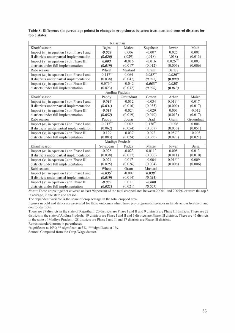
35
Table 8: Difference (in percentage points) in change in crop shares between treatment and control districts for top 3 states
RajasthanKharif season Bajra Maize Soyabean Jowar MothImpact ( in equation 1) on Phase I and II districts under partial implementation
-0.009(0.020)
0.006(.029)
-0.007(.018)
0.025(.018)
0.001(0.013)
Impact ( in equation 2) on Phase III districts under full implementation
0.003(0.019)
-0.016(0.017)
-0.016(0.012)
0.026***
(0.006)0.003
(0.006)Rabi season Wheat Mustard Gram Barley Impact ( in equation 1) on Phase I and II districts under partial implementation
-0.117**
(0.038)0.064
(0.047)0.087**
(0.032)-0.029**
(0.009)Impact ( in equation 2) on Phase III districts under full implementation
0.076**
(0.023)-0.042(0.032)
-0.063**
(0.020)0.025*
(0.013)Andhra Pradesh
Kharif season Paddy Groundnut Cotton Arhar Maize Impact ( in equation 1) on Phase I and II districts under partial implementation
-0.016(0.031)
-0.012(0.016)
-0.034(0.035)
0.019**
(0.009)0.017
(0.017)Impact ( in equation 2) on Phase III districts under full implementation
-0.018(0.057)
-0.024(0.019)
-0.029(0.040)
0.003(0.013)
-0.012(0.017)
Rabi season Paddy Jowar Urad Gram GroundnutImpact ( in equation 1) on Phase I and II districts under partial implementation
-0.215**
(0.062)0.002
(0.054)0.156**
(0.057)-0.006(0.030)
0.004(0.051)
Impact ( in equation 2) on Phase III districts under full implementation
-0.129(0.083)
-0.037(0.024)
0.092(0.060)
0.059**
(0.023)-0.003(0.021)
Madhya PradeshKharif season Soyabean Paddy Maize Jowar BajraImpact ( in equation 1) on Phase I and II districts under partial implementation
-0.028(0.038)
-0.023(0.017)
0.011*
(0.006)0.008
(0.011)0.013
(0.010)Impact ( in equation 2) on Phase III districts under full implementation
-0.024(0.025)
0.017(0.026)
-0.004(0.004)
0.016**
(0.006)0.009
(0.006)Rabi season Wheat Gram Mustard Impact ( in equation 1) on Phase I and II districts under partial implementation
-0.035*
(0.019)-0.007(0.014)
0.038*
(0.021)Impact ( in equation 2) on Phase IIIdistricts under full implementation
-0.005(0.021)
0.011(0.021)
-0.008(0.007)
Notes: These crops together covered at least 90 percent of the total cropped area between 2000/1 and 2005/6, or were the top 5 in acreage, in the state and season.The dependent variable is the share of crop acreage in the total cropped area. Figures in bold and italics are presented for those outcomes which have pre-program differences in trends across treatment and control districts. There are 29 districts in the state of Rajasthan: 20 districts are Phase I and II and 9 districts are Phase III districts. There are 22 districts in the state of Andhra Pradesh: 19 districts are Phase I and II and 3 districts are Phase III districts. There are 45 districts in the state of Madhya Pradesh: 28 districts are Phase I and II and 17 districts are Phase III districts. Robust standard errors in parentheses.*significant at 10%; ** significant at 5%; ***significant at 1%.Source: Computed from the Crop-Wage dataset.

36
Table 9: Difference (in percentage points over time) in rates of growth in crop yields between treatment and control districts
RajasthanKharif season Bajra Maize Soyabean Jowar MothImpact ( in equation 1) on Phase I and II districts under partialimplementation
-0.33**
(0.12)-0.08(0.11)
0.12(0.12)
-0.54*
(0.28)1.05**
(0.39)
Impact ( in equation 2) on Phase IIIdistricts under full implementation
-0.46(0.59)
-0.46(0.30)
-0.22**
(0.10)-0.38(0.92)
0.18(0.58)
Rabi season Wheat Mustard Gram Barley Impact ( in equation 1) on Phase I and II districts under partialimplementation
-0.00(0.10)
0.23(0.14)
-0.02(0.16)
0.03(0.08)
Impact ( in equation 2) on Phase IIIdistricts under full implementation
0.04(0.07)
0.13(0.20)
0.17(0.18)
0.07(0.12)
Andhra PradeshKharif season Paddy Groundnut Cotton Arhar MaizeImpact ( in equation 1) on Phase I and II districts under partialimplementation
0.02(0.08)
0.84***
(0.01)-0.07(0.34)
-0.65**
(0.27)0.05
(0.27)
Impact ( in equation 2) on Phase IIIdistricts under full implementation
-0.04(0.12)
-0.19(0.50)
-0.24(0.30)
-0.18(0.30)
-0.16(0.37)
Rabi season Paddy Jowar Urad Gram GroundnutImpact ( in equation 1) on Phase I and II districts under partialimplementation
-0.12(0.09)
na -0.49**
(0.17)na 0.21*
(0.11)
Impact ( in equation 2) on Phase IIIdistricts under full implementation
-0.14(0.09)
na -0.27(0.32)
na -0.19**
(0.09)
Madhya PradeshKharif season Soyabean Paddy Maize Jowar BajraImpact ( in equation 1) on Phase I and II districts under partialimplementation
-0.10(0.12)
-0.05(0.14)
0.12(0.08)
0.09(0.07)
-0.13(0.10)
Impact ( in equation 2) on Phase IIIdistricts under full implementation
-0.10(0.09)
0.14(0.30)
-0.01(0.06)
0.03(0.09)
0.46(0.46)
Rabi season Wheat Gram Mustard Impact ( in equation 1) on Phase I and II districts under partialimplementation
0.21**
(0.07)0.06
(0.07)0.14*
(0.08)
Impact ( in equation 2) on Phase IIIdistricts under full implementation
0.07(0.07)
0.06(0.07)
-0.06(0.06)
Notes: These crops together covered at least 90 percent of the total cropped area between 2000/1 and 2005/6, or were the top 5 in acreage, in the state and season.The dependent variable is the logarithm of crop yield.Figures in bold and italics are presented for those outcomes which have pre-program differences in trends across treatment and control districts.There are 29 districts in the state of Rajasthan: 20 districts are Phase I and II and 9 districts are Phase III districts. There are 22 districts in the state of Andhra Pradesh: 19 districts are Phase I and II and 3 districts are Phase III districts. There are 45 districts in the state of Madhya Pradesh: 28 districts are Phase I and II and 17 districts are Phase III districts.“na” means not applicable (as the sample is too small)Robust standard errors in parentheses.
*significant at 10%; ** significant at 5%; ***significant at 1%
Source: Computed from the Crop-Wage dataset.

37
Table 10: Summary statistics on real wages (in INR per day in 2004/5 prices)
Casual agriculture Casual non-agriculture Regular agriculture Regular non-agriculture Public works
Mean No. of individuals Mean No. of individuals Mean No. of individuals Mean No. of individuals Mean No. of individuals
Males2004/5 All India (19 States) 49 10748 71 7754 73 818 149 9459 84 177
Phase I and II districts (a) 45 6570 61 4259 78 400 155 4969 98 108Phase III districts (b) 56 4178 84 3495 68 418 143 4490 61 69Difference (a)-(b) -10*** -23*** 10** 12*** 37
2007/8 All India (19 States) 55 16721 78 8806 76 691 151 7083 64 739Phase I and II districts (c) 52 11259 69 5616 68 407 149 3568 63 621Phase III districts (d) 62 5462 91 3190 86 284 153 3515 68 118Difference (c)-(d) -10*** -22*** -17** -3 -5**
2011/12 All India (19 States) 74 5168 98 8756 88 273 179 8785 68 755Phase I and II districts (e) 70 3304 87 5037 88 131 183 4500 68 555Phase III districts (f) 81 1864 114 3719 89 142 174 4285 66 200Difference (e)-(f) -10*** -27*** -1 9** 2
Females2004/5 All India (19 States) 34 7287 45 1331 55 208 89 2146 49 87
Phase I and II districts (a) 32 4589 41 756 58 100 82 1098 48 55Phase III districts (b) 37 2698 50 575 51 108 96 1048 51 32Difference (a)-(b) -4*** -9*** 7 -14** -3
2007/8 All India (19 States) 40 9752 53 1414 51 141 93 1689 61 434Phase I and II districts (c) 39 6521 50 931 46 79 92 825 60 360Phase III districts (d) 42 3231 59 483 59 62 94 864 67 74Difference (c)-(d) -3*** -9*** -13 -1 -7***
2011/12 All India (19 States) 54 3378 65 1037 56 110 113 2046 59 802Phase I and II districts (e) 53 2080 61 574 63 41 113 1053 58 438Phase III districts (f) 56 1298 71 463 49 69 113 993 59 364Difference (e)-(f) -3*** -10*** 14** 0 -1
Notes: The sample comprises of 484 districts: 277-Phase I and II district and 207-Phase III district. Wages calculated using current daily activity (CDS) status, expressed in 2004/5 prices *significant at 10%; ** significant at 5%; ***significant at 1%.Source: NSS-EUS dataset.

38
Table 11.1: Summary statistics on time shares (in fractions of unit time) for malesAgriculture Non-agriculture Public
works Domestic work Unemployment
Not in labour force
No. of IndividualsSelf Regular Casual Self Regular Casual
2004/5 All India (19 States) 0.368 0.009 0.153 0.145 0.079 0.076 0.002 0.013 0.073 0.081Phase I and II districts (a) 0.38 0.008 0.165 0.145 0.064 0.071 0.002 0.016 0.069 0.08 51180Phase III districts (b) 0.35 0.01 0.135 0.146 0.103 0.083 0.002 0.01 0.078 0.084 36491Difference (a)-(b) 0.031*** -0.002*** 0.030*** -0.001 -0.040*** -0.012*** 0 0.006*** -0.009*** -0.004**
2007/8 All India (19 States) 0.345 0.008 0.173 0.133 0.08 0.084 0.007 0.012 0.074 0.084Phase I and II districts (c) 0.351 0.008 0.186 0.132 0.063 0.084 0.01 0.013 0.078 0.075 52532Phase III districts (d) 0.335 0.009 0.153 0.134 0.106 0.085 0.003 0.011 0.069 0.097 31300Difference (c)-(d) 0.016*** -0.002** 0.033*** -0.002 -0.042*** -0.001 0.007*** 0.003*** 0.009*** -0.021***
2011/12 All India (19 States) 0.327 0.004 0.151 0.138 0.088 0.114 0.012 0.01 0.047 0.109Phase I and II districts (e) 0.33 0.004 0.173 0.139 0.07 0.11 0.016 0.01 0.045 0.103 37680Phase III districts (f) 0.323 0.006 0.117 0.135 0.117 0.119 0.006 0.008 0.051 0.118 26902Difference (e)-(f) 0.007* -0.002*** 0.056*** 0.004 -0.046*** -0.009*** 0.010*** 0.002** -0.006*** -0.015***Notes: The sample comprises of 484 districts: 277 Phase I and II, and 207 Phase III districts. Time shares have been estimated using current daily activity (CDS) status.*significant at 10%; ** significant at 5%; ***significant at 1%.
Table 11.2: Summary statistics on time shares (in fractions of unit time) for femalesAgriculture Non-agriculture Public
worksDomestic
work Unemployment Not in labour force Individuals
Self Regular Casual Self Regular Casual2004/5 All India (19 States) 0.192 0.002 0.088 0.04 0.018 0.013 0.001 0.563 0.035 0.047
Phase I and II districts (a) 0.182 0.002 0.092 0.041 0.015 0.012 0.001 0.576 0.032 0.047 52194Phase III districts (b) 0.209 0.003 0.082 0.038 0.024 0.014 0.001 0.541 0.04 0.048 36615Difference (a)-(b) -0.027*** -0.001 0.011*** 0.002* -0.009*** -0.002** 0 0.035*** -0.008*** -0.001
2007/8 All India (19 States) 0.149 0.002 0.09 0.029 0.019 0.013 0.005 0.623 0.027 0.044Phase I and II districts (c) 0.144 0.002 0.094 0.029 0.014 0.014 0.006 0.629 0.027 0.041 54446Phase III districts (d) 0.159 0.002 0.082 0.03 0.025 0.013 0.002 0.614 0.026 0.048 32946Difference (c)-(d) -0.015*** 0 0.013*** -0.001 -0.011*** 0.001 0.005*** 0.015*** 0.001 -0.007***
2011/12 All India (19 States) 0.125 0.002 0.067 0.032 0.021 0.014 0.01 0.649 0.017 0.063Phase I and II districts (e) 0.115 0.001 0.071 0.034 0.016 0.013 0.01 0.666 0.014 0.059 38033Phase III districts (f) 0.142 0.002 0.06 0.03 0.029 0.016 0.01 0.621 0.021 0.07 27420Difference (e)-(f) -0.026*** -0.001** 0.011*** 0.004** -0.013*** -0.003** 0 0.046*** -0.007*** -0.011***Notes: The sample comprises of 484 districts: 277-Phase I and II districts and 207-Phase III districts Time shares have been estimated using current daily activity (CDS) status. *significant at 10%; ** significant at 5%; ***significant at 1%.
Source for both tables: Computed from the NSS-EUS dataset.

39
Table 12.1: Difference (in percentage points over time) in rates of growth in real casual wages between treatment and control districts, top 3 states (Rajasthan, Andhra Pradesh and Madhya Pradesh)
Male FemaleRainyseason
No. of individuals
DrySeason
No. of individuals
Rainyseason
No. of individuals
Dryseason
No. of individuals
Average casual wages in agriculture sector (INR per day in 2004/5 prices)Phase I and II districts in 2004/5 43 673 43 645 30 805 31 656Phase III districts in 2004/5 41 237 37 211 33 153 28 121
Impact on real casual wages in agriculture sectorImpact ( in equation 1) on Phase I and II districts under partial implementation
0.040(0.030)
2451 0.058(0.052)
2194 0.161**
(0.055) 2321 -0.043(0.069)
1910
Impact ( in equation 2) on Phase IIIdistricts under full implementation
0.038(0.067)
1935 0.018(0.060)
1683 0.260**
(0.090) 1845 -0.066(0.077)
1543
Average casual wages in non-agriculture sector (INR per day in 2004/5 prices)Phase I and II districts in 2004/5 58 444 57 510 44 101 43 117Phase III districts in 2004/5 57 108 59 171 35 12 39 42
Impact on real casual wages in non-agriculture sectorImpact ( in equation 1) on Phase I and II districts under partial implementation
0.161***
(0.046)1151 -0.021
(0.051)1523 -1.044**
(0.390) 241 0.018(0.261)
401
Impact ( in equation 2) on Phase IIIdistricts under full implementation
0.029(0.051)
1181 -0.132**
(0.064)1556 -0.179
(0.176) 234 -0.071(0.099)
395
Notes: The dependent variable is logarithm of casual wage in agriculture. All the regressions have been performed using modified individual level weights derived from district level matching weights, in the common support region. The common support region comprises of 81 districts out of 97 districts.Figures in bold and italics are presented for those outcomes which have pre-program differences in trends across treatment and control districts.
Standard errors clustered at the district-year level in parentheses. *significant at 10%; ** significant at 5%; ***significant at 1%.
Source: Computed from the NSS-EUS dataset.

40
Table 12.2: Impact on time shares for males, top 3 states (Rajasthan, Andhra Pradesh and Madhya Pradesh)Agriculture Non-agriculture Public
worksDomestic
work UnemploymentNot in labour forceSelf Regular Casual Self Regular Casual
Average time shares in rainy season (fraction of unit time)Phase I and II districts in 2004/5 0.417 0.009 0.154 0.130 0.067 0.076 0.001 0.006 0.060 0.080Phase III districts in 2004/5 0.407 0.009 0.164 0.090 0.102 0.060 0.011 0.027 0.069 0.062
Rainy season impact estimates: Difference in change in time shares between treatment and control districtsImpact ( in equation 1) on Phase I and II districts under partial implementation
-0.031(0.020)
0.005(0.004)
-0.001(0.016)
-0.011(0.009)
0.052***
(0.014)0.010
(0.008)0.015**
(0.005)0.004
(0.004)-0.023(0.025)
-0.020**
(0.008)Impact ( in equation 2) on Phase IIIdistricts under full implementation
0.047(0.033)
-0.004(0.005)
-0.032(0.025)
0.037**
(0.015)-0.023*
(0.012)0.002
(0.021)0.001
(0.005)0.009
(0.007)0.001
(0.012)-0.038***
(0.011)Average time shares in dry season (fraction of unit time)
Phase I and II districts in 2004/5 0.376 0.014 0.161 0.126 0.076 0.089 0.007 0.007 0.072 0.071Phase III districts in 2004/5 0.415 0.004 0.176 0.118 0.061 0.055 0.002 0.019 0.082 0.067
Dry season impact estimates: Difference in change in time shares between treatment and control districtsImpact ( in equation 1) on Phase I and II districts under partial implementation
0.124***
(0.027)-0.011**
(0.003)-0.084**
(0.026)0.016
(0.011)-0.025**
(0.012)-0.033**
(0.015)0.016**
(0.008)-0.003(0.005)
-0.014(0.014)
0.013(0.008)
Impact ( in equation 2) on Phase IIIdistricts under full implementation
0.099**
(0.035)-0.001(0.003)
0.028(0.024)
-0.049**
(0.019)-0.031(0.021)
-0.032(0.021)
0.008(0.012)
-0.009*
(0.005)-0.029*
(0.015)0.015
(0.015)Notes: The dependent variable is the fraction of unit time spent in a particular activity. All the regressions have been performed using modified individual level weights derived from district level matching weights, in the common support region. The common support region comprises of 81 districts out of 97 districts.Figures in bold and italics are presented for those outcomes which have pre-program differences in trends across treatment and control districts. Standard errors clustered at the district-year level in parentheses. *significant at 10%; ** significant at 5%; ***significant at 1%.
Source: Computed from the NSS-EUS dataset.
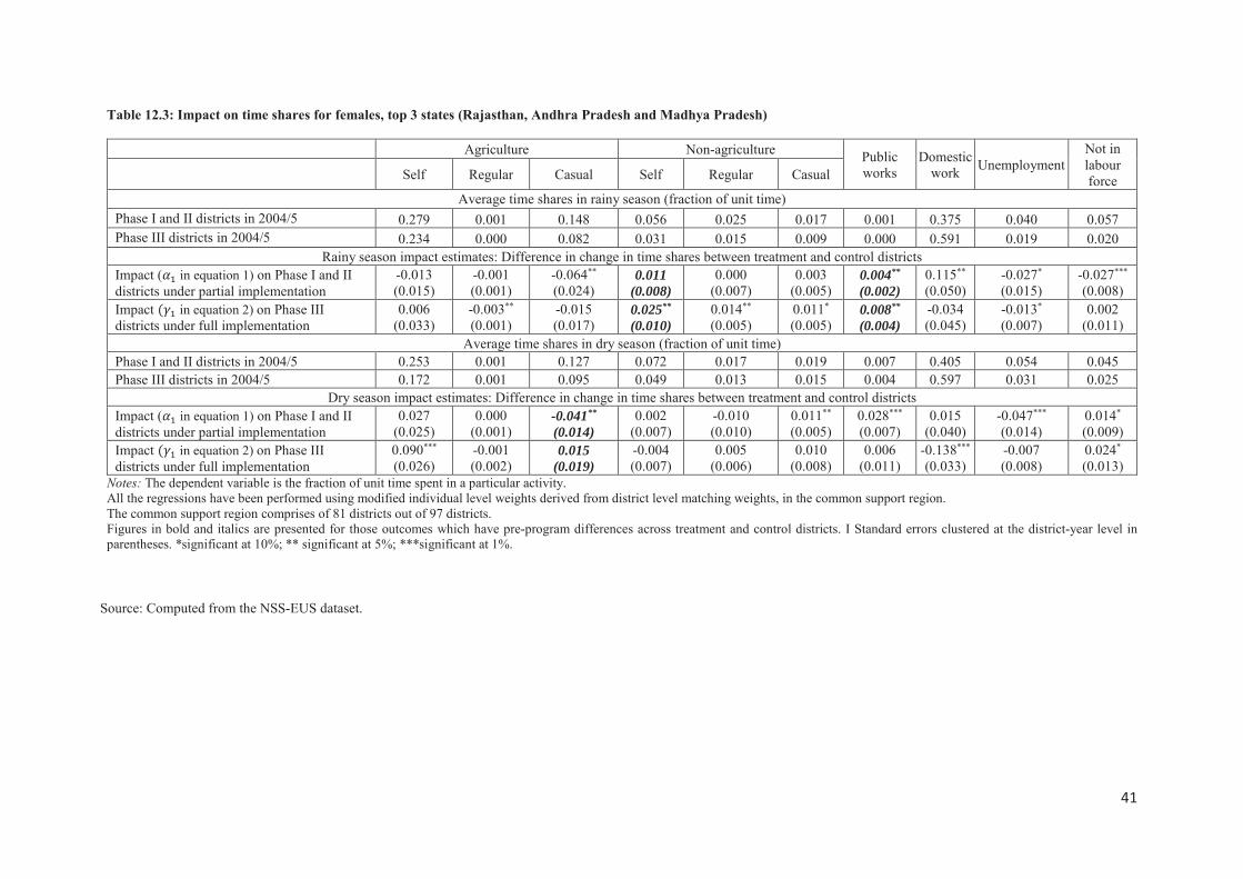
41
Table 12.3: Impact on time shares for females, top 3 states (Rajasthan, Andhra Pradesh and Madhya Pradesh)
Agriculture Non-agriculture Public works
Domestic work Unemployment
Not in labour forceSelf Regular Casual Self Regular Casual
Average time shares in rainy season (fraction of unit time)Phase I and II districts in 2004/5 0.279 0.001 0.148 0.056 0.025 0.017 0.001 0.375 0.040 0.057Phase III districts in 2004/5 0.234 0.000 0.082 0.031 0.015 0.009 0.000 0.591 0.019 0.020
Rainy season impact estimates: Difference in change in time shares between treatment and control districtsImpact ( in equation 1) on Phase I and II districts under partial implementation
-0.013(0.015)
-0.001(0.001)
-0.064**
(0.024)0.011
(0.008)0.000
(0.007)0.003
(0.005)0.004**
(0.002)0.115**
(0.050)-0.027*
(0.015)-0.027***
(0.008)Impact ( in equation 2) on Phase IIIdistricts under full implementation
0.006(0.033)
-0.003**
(0.001)-0.015(0.017)
0.025**
(0.010)0.014**
(0.005)0.011*
(0.005)0.008**
(0.004)-0.034(0.045)
-0.013*
(0.007)0.002
(0.011)Average time shares in dry season (fraction of unit time)
Phase I and II districts in 2004/5 0.253 0.001 0.127 0.072 0.017 0.019 0.007 0.405 0.054 0.045Phase III districts in 2004/5 0.172 0.001 0.095 0.049 0.013 0.015 0.004 0.597 0.031 0.025
Dry season impact estimates: Difference in change in time shares between treatment and control districtsImpact ( in equation 1) on Phase I and II districts under partial implementation
0.027(0.025)
0.000(0.001)
-0.041**
(0.014)0.002
(0.007)-0.010(0.010)
0.011**
(0.005)0.028***
(0.007)0.015
(0.040)-0.047***
(0.014)0.014*
(0.009)Impact ( in equation 2) on Phase IIIdistricts under full implementation
0.090***
(0.026)-0.001(0.002)
0.015(0.019)
-0.004(0.007)
0.005(0.006)
0.010(0.008)
0.006(0.011)
-0.138***
(0.033)-0.007(0.008)
0.024*
(0.013)Notes: The dependent variable is the fraction of unit time spent in a particular activity. All the regressions have been performed using modified individual level weights derived from district level matching weights, in the common support region. The common support region comprises of 81 districts out of 97 districts.Figures in bold and italics are presented for those outcomes which have pre-program differences across treatment and control districts. I Standard errors clustered at the district-year level in parentheses. *significant at 10%; ** significant at 5%; ***significant at 1%.
Source: Computed from the NSS-EUS dataset.

42
Table 13.1: Difference (in percentage points over time) in rates of growth in real casual wages between treatment and control districts, all-India
Male FemaleRainyseason
No. of individuals
Dryseason
No. of individuals
Rainyseason
No. of individuals
Dryseason
No. of individuals
Average casual wages in agriculture sector (INR per day in 2004/5 prices)Phase I and II districts in 2004/5 46 2233 47 2007 31 2113 32 1638Phase III districts in 2004/5 46 2056 47 1901 32 1396 34 1233
Impact on real casual wages in agriculture sectorImpact ( in equation 1) on Phase I and II districts under partial implementation
-0.015(0.022) 10412 0.002
(0.032) 9653 0.020(0.026) 7886 -0.006
(0.038) 6699
Impact ( in equation 2) on Phase IIIdistricts under full implementation
0.035(0.029)
8246 -0.045(0.031)
7611 0.020(0.038) 6122 -0.130**
(0.043)5192
Average casual wages in non-agriculture sector (INR per day in 2004/5 prices)Phase I and II districts in 2004/5 43 292 61 1675 41 245 65 1318Phase III districts in 2004/5 41 304 67 1670 45 239 64 1534
Impact on real casual wages in non-agriculture sectorImpact ( in equation 1) on Phase I and II districts under partial implementation
-0.040(0.035) 5808 0.008
(0.027) 6958 -0.220*
(0.122) 928 -0.010(0.148) 1316
Impact ( in equation 2) on Phase IIIdistricts under full implementation
-0.002(0.033)
6218 0.014(0.028)
7258 0.227*
(0.119) 897 -0.065(0.073)
1169
Notes: The dependent variable is logarithm of casual wage in agriculture. All the regressions have been performed using modified individual level weights derived from district level matching weights, in the common support region.The common support region comprises of 391 districts out of 484 districts. Figures in bold and italics are presented for those outcomes which have pre-program differences in trends across treatment and control districts.Standard errors clustered at the district-year level in parentheses. *significant at 10%; ** significant at 5%; ***significant at 1%.
Source: Computed from the NSS-EUS dataset.
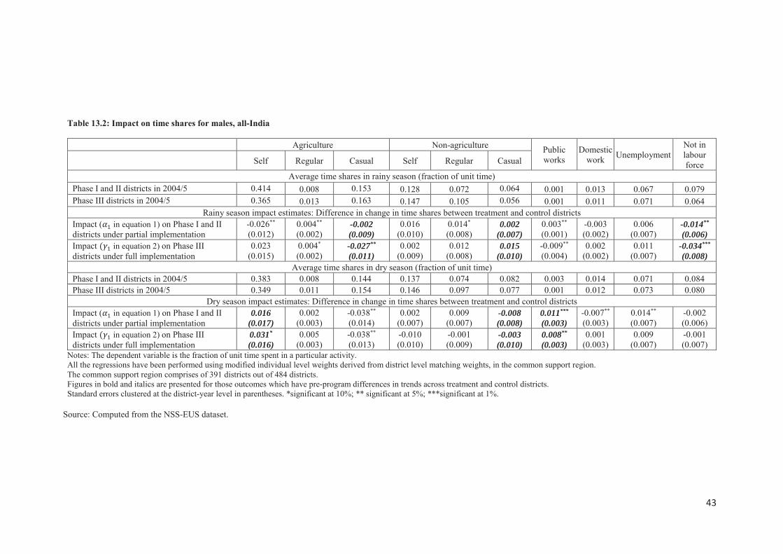
43
Table 13.2: Impact on time shares for males, all-India
Agriculture Non-agriculture Public works
Domestic work Unemployment
Not in labour forceSelf Regular Casual Self Regular Casual
Average time shares in rainy season (fraction of unit time)Phase I and II districts in 2004/5 0.414 0.008 0.153 0.128 0.072 0.064 0.001 0.013 0.067 0.079Phase III districts in 2004/5 0.365 0.013 0.163 0.147 0.105 0.056 0.001 0.011 0.071 0.064
Rainy season impact estimates: Difference in change in time shares between treatment and control districtsImpact ( in equation 1) on Phase I and II districts under partial implementation
-0.026**
(0.012)0.004**
(0.002)-0.002(0.009)
0.016(0.010)
0.014*
(0.008)0.002
(0.007)0.003**
(0.001)-0.003(0.002)
0.006(0.007)
-0.014**
(0.006)Impact ( in equation 2) on Phase IIIdistricts under full implementation
0.023(0.015)
0.004*
(0.002)-0.027**
(0.011)0.002
(0.009)0.012
(0.008)0.015
(0.010)-0.009**
(0.004)0.002
(0.002)0.011
(0.007)-0.034***
(0.008)Average time shares in dry season (fraction of unit time)
Phase I and II districts in 2004/5 0.383 0.008 0.144 0.137 0.074 0.082 0.003 0.014 0.071 0.084Phase III districts in 2004/5 0.349 0.011 0.154 0.146 0.097 0.077 0.001 0.012 0.073 0.080
Dry season impact estimates: Difference in change in time shares between treatment and control districtsImpact ( in equation 1) on Phase I and II districts under partial implementation
0.016(0.017)
0.002(0.003)
-0.038**
(0.014)0.002
(0.007)0.009
(0.007)-0.008(0.008)
0.011***
(0.003)-0.007**
(0.003)0.014**
(0.007)-0.002(0.006)
Impact ( in equation 2) on Phase IIIdistricts under full implementation
0.031*
(0.016)0.005
(0.003)-0.038**
(0.013)-0.010(0.010)
-0.001(0.009)
-0.003(0.010)
0.008**
(0.003)0.001
(0.003)0.009
(0.007)-0.001(0.007)
Notes: The dependent variable is the fraction of unit time spent in a particular activity. All the regressions have been performed using modified individual level weights derived from district level matching weights, in the common support region. The common support region comprises of 391 districts out of 484 districts.Figures in bold and italics are presented for those outcomes which have pre-program differences in trends across treatment and control districts. Standard errors clustered at the district-year level in parentheses. *significant at 10%; ** significant at 5%; ***significant at 1%.
Source: Computed from the NSS-EUS dataset.

44
Table 13.3: Impact on time shares for females, all-India
Agriculture Non-agriculture Public works
Domestic work Unemployment
Not in labour forceSelf Regular Casual Self Regular Casual
Average time shares in rainy season (fraction of unit time)Phase I and II districts in 2004/5 0.239 0.001 0.121 0.038 0.019 0.012 0.001 0.483 0.035 0.051Phase III districts in 2004/5 0.206 0.003 0.109 0.037 0.017 0.009 0.000 0.549 0.027 0.042
Rainy season impact estimates: Difference in change in time shares between treatment and control districtsImpact ( in equation 1) on Phase I and II districts under partial implementation
-0.013(0.010)
-0.002(0.002)
-0.005(0.009)
0.006(0.005)
-0.005(0.003)
0.003*
(0.002)0.001**
(0.001)0.023
(0.014)-0.006(0.004)
-0.003(0.004)
Impact ( in equation 2) on Phase IIIdistricts under full implementation
0.006(0.012)
0.005**
(0.002)0.016**
(0.007)-0.001(0.004)
-0.002(0.005)
0.004(0.003)
-0.002(0.002)
-0.036**
(0.016)0.015**
(0.005)-0.006(0.006)
Average time shares in dry season (fraction of unit time)Phase I and II districts in 2004/5 0.208 0.001 0.095 0.045 0.016 0.015 0.002 0.521 0.045 0.051Phase III districts in 2004/5 0.181 0.005 0.085 0.045 0.024 0.019 0.004 0.560 0.039 0.039
Dry season impact estimates: Difference in change in time shares between treatment and control districtsImpact ( in equation 1) on Phase I and II districts under partial implementation
-0.001(0.013)
0.004**
(0.002)-0.013(0.009)
-0.002(0.006)
0.004(0.004)
0.008**
(0.003)0.013***
(0.003)0.001
(0.021)-0.008(0.008)
-0.007(0.005)
Impact ( in equation 2) on Phase IIIdistricts under full implementation
0.038***
(0.011)0.001*
(0.001)-0.011(0.007)
-0.004(0.007)
0.005(0.003)
0.004(0.003)
0.006(0.005)
-0.046**
(0.017)0.010**
(0.005)-0.003(0.006)
Notes: The dependent variable is the fraction of unit time spent in a particular activity. All the regressions have been performed using modified individual level weights derived from district level matching weights, in the common support region. The common support region comprises of 391 districts out of 484 districts.Figures in bold and italics are presented for those outcomes which have pre-program differences in trends across treatment and control districts.Standard errors clustered at the district-year level in parentheses. *significant at 10%; ** significant at 5%; ***significant at 1%.
Source: Computed from the NSS-EUS dataset.
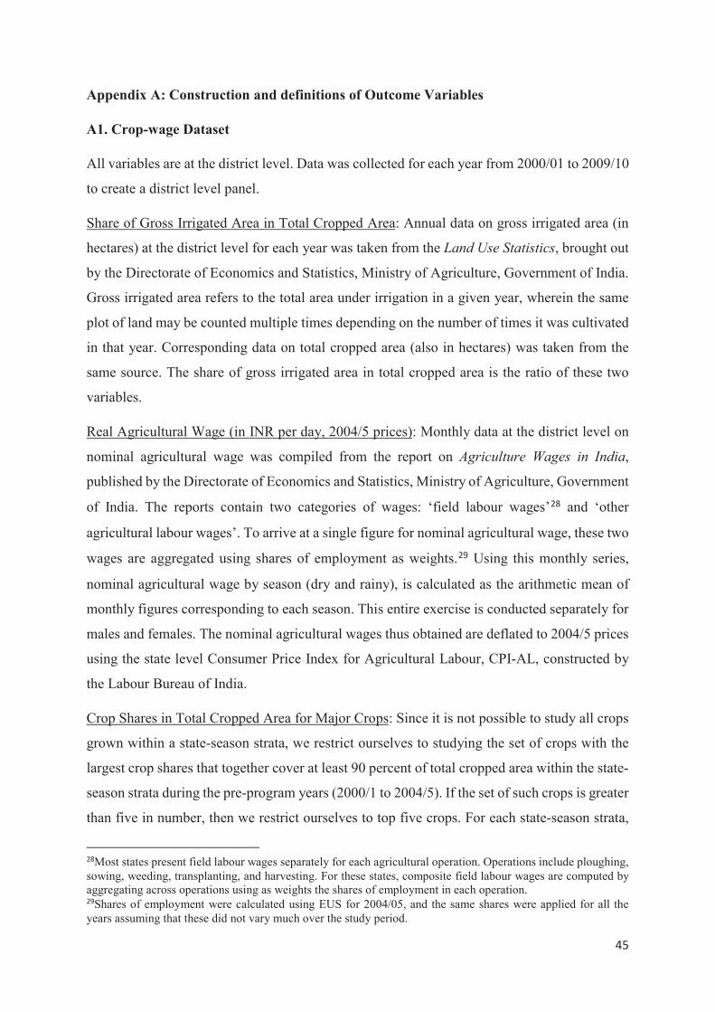
45
Appendix A: Construction and definitions of Outcome Variables
A1. Crop-wage Dataset
All variables are at the district level. Data was collected for each year from 2000/01 to 2009/10
to create a district level panel.
Share of Gross Irrigated Area in Total Cropped Area: Annual data on gross irrigated area (in
hectares) at the district level for each year was taken from the Land Use Statistics, brought out
by the Directorate of Economics and Statistics, Ministry of Agriculture, Government of India.
Gross irrigated area refers to the total area under irrigation in a given year, wherein the same
plot of land may be counted multiple times depending on the number of times it was cultivated
in that year. Corresponding data on total cropped area (also in hectares) was taken from the
same source. The share of gross irrigated area in total cropped area is the ratio of these two
variables.
Real Agricultural Wage (in INR per day, 2004/5 prices): Monthly data at the district level on
nominal agricultural wage was compiled from the report on Agriculture Wages in India,
published by the Directorate of Economics and Statistics, Ministry of Agriculture, Government
of India. The reports contain two categories of wages: ‘field labour wages’28 and ‘other
agricultural labour wages’. To arrive at a single figure for nominal agricultural wage, these two
wages are aggregated using shares of employment as weights.29 Using this monthly series,
nominal agricultural wage by season (dry and rainy), is calculated as the arithmetic mean of
monthly figures corresponding to each season. This entire exercise is conducted separately for
males and females. The nominal agricultural wages thus obtained are deflated to 2004/5 prices
using the state level Consumer Price Index for Agricultural Labour, CPI-AL, constructed by
the Labour Bureau of India.
Crop Shares in Total Cropped Area for Major Crops: Since it is not possible to study all crops
grown within a state-season strata, we restrict ourselves to studying the set of crops with the
largest crop shares that together cover at least 90 percent of total cropped area within the state-
season strata during the pre-program years (2000/1 to 2004/5). If the set of such crops is greater
than five in number, then we restrict ourselves to top five crops. For each state-season strata,
28Most states present field labour wages separately for each agricultural operation. Operations include ploughing, sowing, weeding, transplanting, and harvesting. For these states, composite field labour wages are computed by aggregating across operations using as weights the shares of employment in each operation.29Shares of employment were calculated using EUS for 2004/05, and the same shares were applied for all the years assuming that these did not vary much over the study period.

46
crop specific acreages (in hectares) at the district level have been taken from the Area
Production and Yield, APY, reports of the Ministry of Agriculture, New Delhi. Corresponding
figures for total cropped area (in hectares), are calculated by summing over all reported crop
acreages. Crop shares are then calculated by taking the ratio of crop specific acreage to total
cropped area.
Crop Yield (in tonnes per hectare): For each state-season, crop yields are studied for the same
set of crops used to study cropping patterns. Within each state-season, district level data for
crop yields are directly reported in the APY reports.
A2. EUS Dataset
For the main analysis, we use EUS rounds for the years 2004/5, 2007/8 and 2011/12. We
created a panel of districts that took into account changes in district boundaries and formation
of new districts. In doing so we dropped districts which split into newer ones that had different
MGNREGA phase designations, and also combined districts from later rounds when they had
the same designation. The basic idea was to drop the least number of observations while
maintaining a clear distinction between early and late phase districts. The exact district
concordance can be obtained on request from the authors. We end up with a panel of 484
districts.
We analyse impacts on employment shares and casual wages. We explain these two outcomes
below.
Employment Shares (in fraction of time spent in each category): For each individual the EUS
collects information on time spent in various activities during the week immediately preceding
the date of the survey. We use this information to calculate the fraction of time spent in the
reference week across ten mutually exclusive and exhaustive employment categories. These
are as follows:
1. Self-employment in agriculture
2. Regular wage employment in agriculture
3. Casual wage employment in agriculture
4. Self-employment in non-agriculture
5. Regular wage employment in non-agriculture
6. Casual wage employment in non-agriculture
7. Wage employment in public works (including MGNREGA)

47
8. Domestic work (free collection of goods, sewing and so on)
9. Unemployment
10. Not in labour force
Note that categories 1 through 6 taken together constitute fraction of time spent in private sector
employment. Categories 8 and 10 when combined constitute fraction of time spent outside the
labour force, defined more broadly to include domestic work.
Causal Wage (in INR per day, 2004/5 prices): In order to separately calculate casual wage in
agriculture and in non-agriculture, we first classify casual work into these two categories using
the National Industrial Classification 1998 (five digit). Using this classification, nominal wages
in each sector is accordingly calculated using information on wage earnings earned and total
days spent in wage employment during the reference week. Wages are then expressed in 2004/5
prices using state level Consumer Price Index for Rural Labour, CPI-RL, constructed by the
Labour Bureau of India.

48
Appendix B: Construction of Weights to Implement Matching
This appendix describes how to modify individual level weights provided by the NSSO to
implement the matching procedure. We describe the procedure to study the effect on Phase I
and II districts using data from 2004/5 and 2007/8. Modified weights for Phase III districts can
be created similarly. The procedure involves two steps.
Step 1: Derivation of District Level Weights using Kernel Matching
Using 2004/5 data, we first run a district level logistic regression to estimate the probability of
receiving the scheme (propensity score) in the early phases, i.e. by 2007/8. The dependent
variable is whether a district is observed to be Phase I / Phase II or not (the variable takes value
1 if it is so, and 0 if it is not). The explanatory variables are all at the district level: these are
share of SC/ST households, average casual wage (2004/5 prices), literacy rate, average land
holding size, average monthly per capita consumption expenditure (2004/5 prices) and state
dummies. The propensity scores of the treatment group (Phase I and II) lie within the interval
[0.050; 0.999], whereas for the control group (Phase III) they lie within [0.001; 0.966].
Therefore, the common support S, is given by all districts whose propensity score lie within
[0.050; 0.966].30 For the rest of the analysis only districts in the common support are
considered.
Suppose there are J Phase I and II treatment districts, t1, t2, …, tJ, and K Phase III control
districts, c1, c2, …, and cK. For each treatment district , we use kernel matching to derive
the set of matching weights { ( , ) = 1, … , }, over the K control districts. Each( , ) depends on the distance between and where is the propensity score, and
is defined as follows:
( , ) = ( )( )where G(u) = (1 u ) is the Epanechnikov kernel function, and h is the bandwidth
parameter.
30Out of 484 (277 Phase I and II, and 207 Phase III) districts considered, 391 districts (81 percent) form the common support, of which 196 are Phase I and II, and 195 are Phase III.
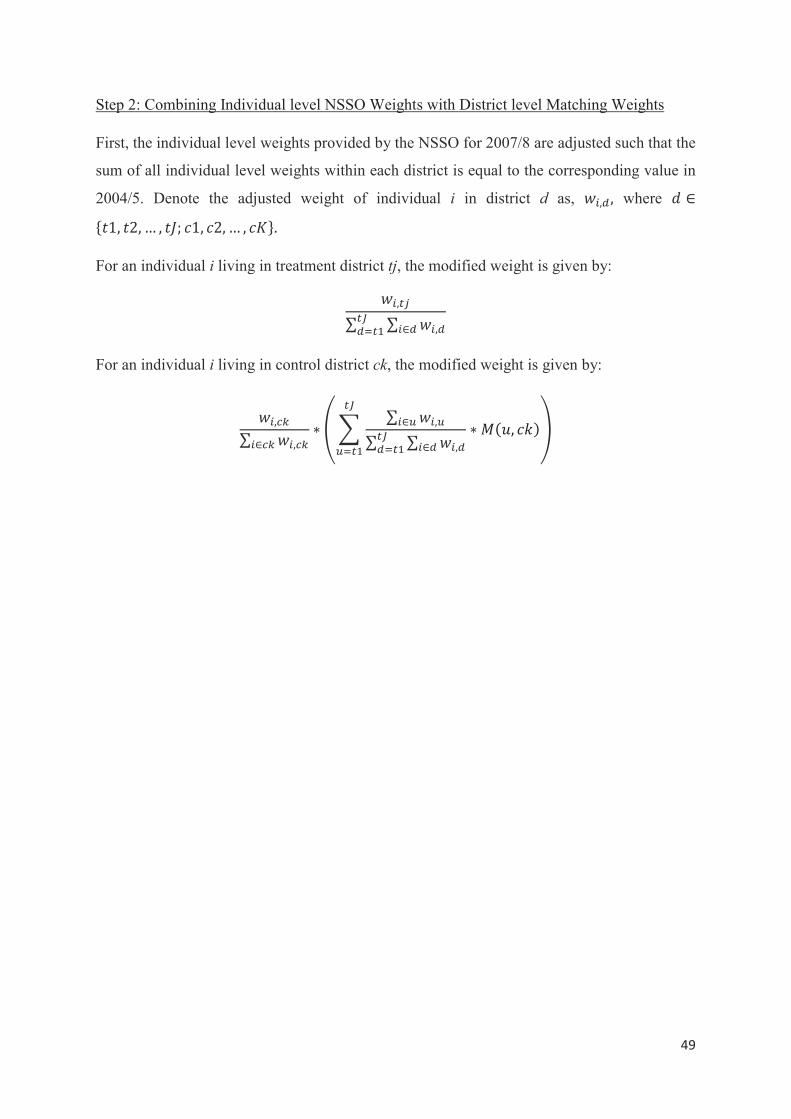
49
Step 2: Combining Individual level NSSO Weights with District level Matching Weights
First, the individual level weights provided by the NSSO for 2007/8 are adjusted such that the
sum of all individual level weights within each district is equal to the corresponding value in
2004/5. Denote the adjusted weight of individual i in district d as, , , where { 1, 2, … , ; 1, 2, … , }.For an individual i living in treatment district tj, the modified weight is given by:
, ,For an individual i living in control district ck, the modified weight is given by:
, , , , ( , )

50
Appendix C
Table C1: Select Characteristics in 2004/5 across Matched and Unmatched Districts
Phase I and II districts
Phase III districts Difference
(a) (b) (a-b)
Unmatched
Share of SC/ST households 0.38 0.28 0.10***Share of literate persons 0.47 0.56 -0.09***Consumer expenditure (INR per month per household) 2412 3030 -618***Casual wage in agriculture sector (INR per day, 2004/5 prices) 46 61 -15***Cultivable land (hectares per household) 1.23 1.48 -0.25**Number of Districts 277 207
MatchedShare of SC/ST households 0.36 0.37 -0.01
Share of literate persons 0.49 0.5 -0.01
Consumer expenditure (INR per month per household) 2533 2593 -60
Casual wage in agriculture sector (INR per day, 2004/5 prices) 47 49 -2
Cultivable land (hectares per household) 1.42 1.34 0.08
Number of Districts (in common support) 196 195Notes: Out of 484 districts, the common support region comprises of 391 districts: 196 Phase I and II and 195 Phase III districts. The propensity scores of the treatment group (Phase I and II) lie within the interval [0.050; 0.999], whereas they lie within [0.001; 0.966] for the control group (Phase III). The common support is given by all districts whose propensity score lie within [0.050; 0.966].

51
Table C2: Labour and water requirement of selected crops
Panel A : Labour requirement (in hours per hectare)
Rajasthan
Rabi crops Wheat Mustard Gram Barley
481 280 229 483
Kharif crops Bajra Maize Soyabean Jowar Moth
290 583 357 250 na
Andhra Pradesh
Rabi crops Paddy Jowar Urad Gram Groundnut
835 424 272 323 642
Kharif crops Paddy Groundnut Cotton Arhar Maize
835 642 824 465 616
Madhya Pradesh
Rabi crops Wheat Gram Mustard
352 238 285
Kharif crops Soyabean Paddy Maize Jowar Bajra
329 540 436 385 na
Panel B: Water requirement (in INR per hectare)
Rajasthan
Rabi crops Wheat Mustard Gram Barley
2936 1651 1383 2706
Kharif crops Bajra Maize Soyabean Jowar Moth
63 43 49 75 na
Andhra Pradesh
Rabi crops Paddy Jowar Urad Gram Groundnut
611 106 0 1 446
Kharif crops Paddy Groundnut Cotton Arhar Maize
611 446 168 0 45
Madhya Pradesh
Rabi crops Wheat Gram Mustard
1879 534 1206
Kharif crops Soyabean Paddy Maize Jowar Bajra
7 210 0 0 naSource: Estimates of cost of cultivation for 2006/7, Directorate of Economics and Statistics, Ministry of Agriculture, Government of India.Notes: ‘na’ means not available.

52
Table C3: Season wise distribution of time shares for casual labour employment in 2007/8
States
Public works Agriculture Non-agriculture
Rainy seasonDry
season
Rainy seasonDry
season
Rainy seasonDry
season
Rajasthan 0.004 0.024 0.034 0.022 0.06 0.101
Andhra Pradesh 0.005 0.025 0.215 0.183 0.046 0.055
Madhya Pradesh 0.003 0.018 0.135 0.137 0.04 0.052
Karnataka na na 0.211 0.215 0.037 0.035
Chhattisgarh 0.002 0.031 0.181 0.127 0.029 0.051
Jharkhand 0.004 0.005 0.052 0.031 0.079 0.118
Tamil Nadu 0.013 0.019 0.17 0.166 0.077 0.072Himachal Pradesh 0.014 0.016 0.011 0.007 0.06 0.063
Assam 0.001 0.004 0.06 0.055 0.032 0.044
Uttar Pradesh 0.005 0.002 0.05 0.052 0.049 0.056
Uttaranchal 0.003 0.007 0.029 0.016 0.04 0.053
West Bengal 0.003 0.008 0.137 0.121 0.052 0.056
Gujarat na na 0.158 0.165 0.042 0.052
Kerala 0.004 0.005 0.05 0.053 0.091 0.101
Orissa 0.003 0.005 0.13 0.08 0.041 0.062
Bihar 0.004 0.005 0.151 0.149 0.028 0.034
Punjab na na 0.067 0.071 0.063 0.061
Haryana 0.002 0.001 0.05 0.057 0.054 0.07
Maharashtra 0.001 0.001 0.199 0.182 0.026 0.041
All states 0.004 0.009 0.125 0.115 0.047 0.058
Source: Employment and Unemployment Survey, National Sample Survey (NSS), 2007/8Note: Target population consists of individuals residing in rural areas, between 18 and 60 years of age, for 19 major states.‘na’ means not available. The states have been arranged according to the ranking of successful MGNREGA implementationgiven in Table 1.