≈√

O e s t e r r e i c h i s c h e Nat i ona l b a n k

W o r k i n g P a p e r 7 9

Risk Assessment for Banking Systems

Helmut Elsinger, Alfred Lehar, Martin Summer

Editorial Board of the Working Papers Eduard Hochreiter, Coordinating Editor Ernest Gnan, Wolfdietrich Grau, Peter Mooslechner Kurt Pribil

Statement of Purpose The Working Paper series of the Oesterreichische Nationalbank is designed to disseminate and to provide a platform for discussion of either work of the staff of the OeNB economists or outside contributors on topics which are of special interest to the OeNB. To ensure the high quality of their content, the contributions are subjected to an international refereeing process. The opinions are strictly those of the authors and do in no way commit the OeNB.

Imprint: Responsibility according to Austrian media law: Wolfdietrich Grau, Secretariat of the Board of Executive Directors, Oesterreichische Nationalbank Published and printed by Oesterreichische Nationalbank, Wien. The Working Papers are also available on our website: http://www.oenb.co.at/workpaper/pubwork.htm

Editorial In this paper, Helmut Elsinger, Alfred Lehar and Martin Summer suggest a new

approach to risk assessment for banks. Rather than looking at them individually

they try to undertake an analysis at the level of the banking system. Such a

perspective is necessary because the complicated network of mutual credit

obligations can make the actual risk exposure of banks invisible at the level of

individual institutions. Using standard risk management techniques in

combination with a network model of interbank exposures, the authors analyze

the consequences of macroeconomic shocks for bank insolvency risk. In

particular, they consider interest rate shocks, exchange rate and stock market

movements as well as shocks related to the business cycle. The feedback

between individual banks and potential domino effects from bank defaults are

taken explicitly into account. The model determines endogenously probabilities

of bank insolvencies, recovery rates and a decomposition of insolvency cases

into defaults that directly result from movements in risk factors and defaults that

arise indirectly as a consequence of contagion.

October 28, 2002

Risk Assessment for Banking Systems∗

Helmut Elsinger†

University of Vienna

Department of Business Studies

Alfred Lehar‡

University of British Columbia

Faculty of Commerce

Martin Summer§

Oesterreichische Nationalbank

Economic Studies Division

First version February 2002This version October 2002

∗We have to thank Ralf Dobringer, Bettina Kunz, Franz Partsch and Gerhard Fiam for their helpand support with the collection of data. We thank Klaus Duellmann, Phil Davis, Eduard Hochreiter,George Kaufman, Markus Knell, David Llewellyn, Matt Pritsker, Christian Upper and Andreas Wormsfor helpful comments. We also thank seminar and conference participants at OeNB, Technical UniversityVienna, Board of Governors of the Federal Reserve System, the IMF, the 2002 WEA meetings, the 2002European Economic Association Meetings, the 2002 European Econometric Association Meetings, andthe CESifo workshop on Financial Regulation and Financial Stability for their comments. The viewsand findings of this papers are entirely those of the authors and do not necessarily represent the views ofOesterreichische Nationalbank.

†Brunner Strasse 71, A-1210 Wien, Austria, e-mail: helmut.elsinger@univie.ac.at, Tel: +43-1-427738057, Fax: +43-1-4277 38054

‡2053 Main Mall, Vancouver, BC, Canada V6T 1Z2, e-mail: alfred.lehar@commerce.ubc.ca, Tel: (604)822 8344, Fax: (604) 822 4695

§corresponding author, Otto-Wagner-Platz 3, A-1011 Wien, Austria, e-mail: mar-tin.summer@oenb.co.at, Tel: +43-1-40420 7212, Fax: +43-1-40420 7299

1

Risk Assessment for Banking Systems

Abstract

In this paper we suggest a new approach to risk assessment for banks. Rather

than looking at them individually we try to undertake an analysis at the level

of the banking system. Such a perspective is necessary because the complicated

network of mutual credit obligations can make the actual risk exposure of banks

invisible at the level of individual institutions. We apply our framework to a cross

section of individual bank data as they are usually collected at the central bank.

Using standard risk management techniques in combination with a network model

of interbank exposures we analyze the consequences of macroeconomic shocks for

bank insolvency risk. In particular we consider interest rate shocks, exchange rate

and stock market movements as well as shocks related to the business cycle. The

feedback between individual banks and potential domino effects from bank defaults

are taken explicitly into account. The model determines endogenously probabilities

of bank insolvencies, recovery rates and a decomposition of insolvency cases into

defaults that directly result from movements in risk factors and defaults that arise

indirectly as a consequence of contagion.

Keywords: Systemic Risk, Interbank Market, Financial Stability, Risk Manage-

ment

JEL-Classification Numbers: G21, C15, C81, E44

2

1 Introduction

Risk management at the level of individual financial institutions has been substantially

improved during the last twenty years. These improvements have been very much spurred

by the pressure to cope with a more volatile and dynamic financial environment after the

breakdown of the Bretton Woods system compared to the postwar period. Pressure has

however not only come from the markets. Regulators have undertaken great efforts since

the eighties to impose new risk management standards on banks. To gain public support

for these measures it has frequently been argued that they are necessary to attenuate

dangers of systemic risk and to strengthen the stability of the financial system. But is

current regulatory and supervisory practice designed appropriately to achieve these goals?

There are reasons to doubt this. Regulators and supervisors are at the moment almost

entirely focused on individual institutions. Assessing the risk of an entire banking system

however requires an approach that goes beyond the individual institution perspective.

One of the major reasons why the individual institutions approach is insufficient is

the fact that modern banking systems are characterized by a fairly complex network of

mutual credit exposures. These credit exposures result from liquidity management on the

one hand and from OTC derivative trading on the other hand. In such a system of mutual

exposures the actual risk borne by the banking system as a whole and the institutions

embedded in it may easily be hidden at the level of an individual bank. The problem of

hidden exposure is perhaps most easily seen in the case of counterparty risk. Judged at

the level of an individual institution it might look rather unspectacular. By the individual

institution perspective it can however remain unnoticed that a bank is part of a chain of

mutual obligations in which credit risks are highly correlated. Its actual risk exposure thus

might indeed be quite substantial. Another example of hidden exposure has been pointed

out in the literature by Hellwig (1995). In Hellwig’s example the network of mutual credit

obligations makes substantial exposure of the system to interest rate risk invisible at the

level of an individual bank because the individual maturity transformation looks short,

whereas the maturity transformation of the system as a whole is rather extreme. To

uncover hidden exposure and to appropriately assess risk in the banking system, rather

than looking at individual institutions, risk assessment should therefore make an attempt

to judge the risk exposure of the system as a whole. A ’system perspective’ on banking

supervision has for instance been actively advocated by Hellwig (1997). Andrew Crockett

(2000), the general manager of the BIS, has even coined a new word - macroprudential -

3

to express the general philosophy of such an approach.1

The open issue then of course is: What exactly does it mean to take a ’system per-

spective’ or a macroprudential viewpoint, for the risk assessment of banks? In our paper

we provide an answer to this question. We develop a methodology to assess the risk of a

banking system taking into account the major macroeconomic risk factors simultaneously

as well as the complex network of interbank dealings. The method is designed in such

a way that it can be applied to data as they are usually collected at a central bank. So

rather than asking what data we would ideally like to have, we want to know how far we

can get with data already available.

Our basic idea is to look at cross sections of individual bank balance sheet and su-

pervisory data from the perspective of a network model describing bilateral interbank

relations in some detail. The model allows us to assess the insolvency risk of banks for

different scenarios of macroeconomic shocks like interest rate shocks, exchange rate and

stock market movements as well as shocks related to the business cycle. Therefore the

contribution of our paper is a risk management model that thinks about the risk expo-

sure of banks at the level of the banking system rather than at the level of individual

institutions. Our approach can thus be seen as an attempt to assess ’systemic risk’.2

1.1 An Overview of the Model

The basic framework is a model of a banking system with a detailed description of the

structure of interbank exposures. The model explains the feasible payment flows between

banks endogenously from a given structure of interbank liabilities, net values of the banks

arising from all other bank activities and an assumption about the resolution of insolvency

in different states of the world. States of the world are described as follows: We expose

the banks financial positions apart from interbank relations to interest rate, exchange

rate, stock market and business cycle shocks. For each state of the world, the network

model uniquely determines endogenously actual interbank payment flows. Taking the

feedback between banks from mutual credit exposures and mutual exposures to aggregate

shocks explicitly into account we can calculate default frequencies of individual banks

1See also Borio (2002).2Note that though the term systemic risk belongs to the standard rhetoric of discussions about banking

regulation it does not have a precise definition (see Summer (2003) for a discussion). We invoke the termhere because we think that our approach captures some of the issues frequently discussed under thisheader, in particular the problem of contagious default.

4

−6 −4 −2 0 2 4 60

5

10

15

20

25

30

������������ ����

����� ������� ������� �! "��� ���#�%$&�')("� �*��+���+,���-�/.0�/+�(!.%�21�3���"4/5767.���5�+���4�82.��!9�+,�

: ;<=> ?@ A

0 1 2 3 4 5 6 7 8 9 100

5

10

15

20

25

B ����CD /E�� ������� ������� �! "��� ���#�%$F6G+H.��I1"+�$J.% !K ���/.0��+

L 4���6G6G���M$J.�4N�����NO

P 4N+H�2.%��� �

Q.%�!5SRT�U�V"W,XZY�[�T

\ ]^_`ab\

Q.%�!5#cT�U�V"WHX�Y�[�T

\ ]^_`ab\

d egf hi j3k e�l!m

n k ego

h e�p n q h e n�r os i h p�t f i t o l

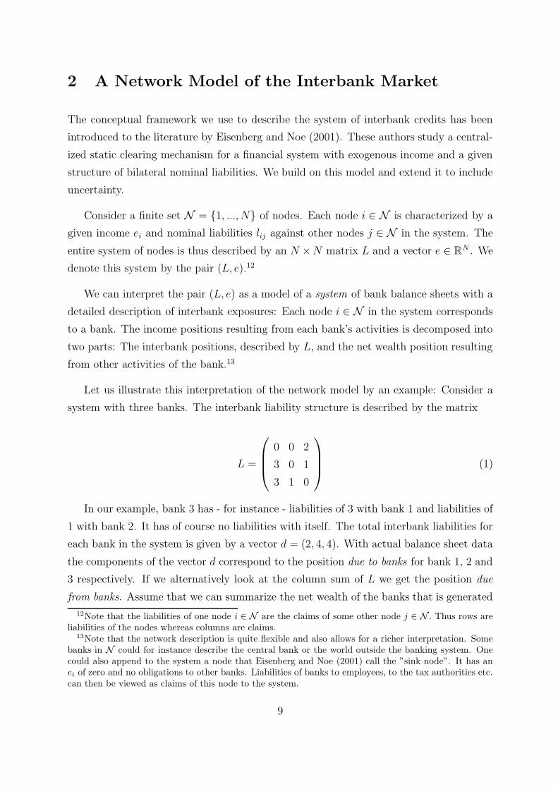
Figure 1. The graph shows the basic structure of the model. Banks are exposed to shocksfrom credit risk and market risk according to their respective exposures. Interbank credit riskis endogenously explained by the network model.

across states. The endogenously determined vector of feasible payments between banks

also determines the recovery rates of banks with exposures to an insolvent counterparty.

We are able to distinguish bank defaults that arise directly as a consequence of move-

ments in the risk factors and defaults which arise indirectly because of contagion. The

model therefore yields a decomposition into fundamental and contagious defaults. Our

approach is illustrated in Figure 1 which shows the various elements of our risk assessment

procedure.

The main data source we use for our model are bank balance sheet data and super-

visory data reported monthly to the Austrian Central Bank (Monatsausweis, MAUS).

In particular these data give us for each bank in the system an aggregate number of on

balance sheet claims and liabilities towards other banks in the system banks abroad and

5

the central bank.3 From this partial information we estimate the matrix of bilateral ex-

posures for the entire system. For the estimation of bilateral exposures we can exploit

information that is revealed by the sectoral organization of the Austrian banking system.4

Scenarios are created by exposing the positions on the balance sheet that are not part of

the interbank business to interest rate, exchange rate, stock market and loan loss shocks.

In order to do so we undertake a historic simulation using market data, except for the

loan losses where we employ a credit risk model. In the scenario part we use data from

Datastream, the major loans statistics produced at the Austrian Central Bank (Großkred-

itevidenz, GKE) as well as statistics of insolvency rates in various industry branches from

the Austrian rating agency Kreditschutzverband von 1870. For each scenario the esti-

mated matrix of bilateral exposures and the income positions determine via the network

model a unique vector of feasible interbank payment and thus a pattern of insolvency. It

is the analysis of these data that we rely on to assess the risk exposure of all banks at a

system level.5

Using a cross section of data for September 2001 we get the following main results:

The Austrian banking system is very stable and default events that could be classified

as a ”systemic crisis” are unlikely. We find that the median default probability of an

Austrian bank to be below one percent. Perhaps the most interesting finding is that only

a small fraction of bank defaults can be interpreted as contagious. The vast majority of

defaults is a direct consequence of macroeconomic shocks. 6 Furthermore we find the

median endogenous recovery rates to be 66%, we show that the Austrian banking system

is quite stable to shocks from losses in foreign counterparty exposure and we find no clear

3Note that these data cover only the on balance sheet part of interbank transactions and do not includeoff balance sheet items.

4The sector organization has mainly historic roots and partitions the banks into joint stock banks,savings banks, state mortgage banks, Raiffeisen Banks, Volksbanken, construction savings and loansassociations and special purpose banks. The system is explained in detail in Section 3.

5Why do we treat the vector income positions apart from interbank dealings as state contingentwhereas we treat the matrix of bilateral exposures as uncontingent? First of all note that the actualinterbank payments are in fact not uncontingent because they are determined by the network model andthus interbank payments vary across states of the world. Treating bilateral exposures as state contingentdirectly with respect to risk factors would mean to have all of them in present values and then to lookat consequences of changes in risk factors such as interest rate risk. Such an analysis is not possible - oronly at the cost of a set of strong and arbitrary assumptions - for the data we have at the moment. Wetherefore treat bilateral interbank exposures by looking at given nominal liabilities and claims as we canreconstruct them from the balance sheet data. As shown in Figure 1 we think of this as a model wherethe income risk of non-interbank positions is driven by exogenous risk factors whereas interbank creditrisk is endogenously explained by the network model.

6This confirms some of the conclusions drawn in a paper by Kaufman (1994) about the empirical(ir)relevance of contagious bank defaults.

6

evidence that the interbank market either increases correlations among banks or enables

banks to diversify risk. Using our model as a simulation tool, we show that market share

in the interbank market alone is not a good predictor of the relevance of a bank for the

banking system.

1.2 Related Research

To our best knowledge this is the first attempt in the literature to design a framework for

the assessment of the risk exposure of an entire banking system taking into account the

detailed micro information usually available in central banks.7 For the different parts of

the model we rely on some results in the literature. The network model we use as the basic

building block is due to Eisenberg and Noe (2001). These authors give an abstract analysis

of a static clearing problem. We rely on these results in the network part of our model. For

our analysis we extend this model to a simple uncertainty framework. The idea to recover

bilateral interbank exposures using bank balance sheet data has first been systematically

pursued by Sheldon and Maurer (1998) for Swiss data on a sectorally aggregated level.

They use an entropy optimization procedure to estimate bilateral exposures from partial

information. Upper and Worms (2002) analyze bank balance sheet data for German

banks. Applying modern techniques from applied mathematics8 they are able to deal with

a much larger problem than Sheldon and Maurer (1998) and estimate bilateral exposures

on a entirely disaggregated level.9 We use similar methods for reconstructing bilateral

exposures for the Austrian data. Using disaggregated data has the advantage that much

of bilateral exposures can be exactly recovered by exploiting structural information about

the banking system under consideration.10 The estimation procedure has then to be

applied only to a relatively small part of exposures for which structural information does

not give any guidelines. The credit risk model we use is a version of the CreditRisk+

7There have however been various theoretical attempts to conceptualize such a problem. These papersare Allen and Gale (2000), Freixas, Parigi, and Rochet (2000), and Dasgupta (2000).

8These techniques are outlined in Blien and Graef (1997) as well as in a book by Fang, Rajasekra,and Tsao (1997).

9Upper and Worms (2002) rely on a combination of exploiting structural information and entropyoptimization for the reconstruction of bilateral exposures.

10This structural information is of course dependent on the country specific features of the reportingsystems. While we can make use of the fact that many banks have to decompose their reports with respectto certain counterparties (see section 4) Upper and Worms (2002) can use the fact that in Germanybanks have to break down their reports between sectors and within this information also with respect tomaturities. Since many banks only borrow or lend in the interbank market at specific maturities theseauthors can identify many bilateral positions.

7

model of Credit Suisse (1997). We have to adapt this framework to deal with a system of

loan portfolios simultaneously rather than with the loan portfolio of a single bank.

There is a related literature that deals with similar questions for payment and banking

systems. Humphery (1986) and Angelini, Maresca, and Russo (1996) deal with settlement

failures in payment systems. Furfine (1999) and Upper and Worms (2002) deal with

banking systems. What is common to all of these studies is that they are concerned with

the contagion of default following the simulated failure of one or more counterparties in

the system. Our study in contrast undertakes a systematic analysis of risk factors and

their impacts on bank income. Bank failures and contagion are studied as a consequence

of these economic shocks to the entire banking system. Thus while the studies cited above

are based on a thought experiment that tries to work out the implications of the structure

of interbank lending on the assumed failure of particular institutions our analysis is built

on a fully fledged model of the banking system’s risk exposure. The consequences of this

exposure is then studied systematically within the framework of the network model. The

main innovation of our model is therefore the combination of a systematic scenario analysis

for risk factors with an analysis of contagious default. We can of course use our framework

to undertake similar simulation exercises as the previous literature on contagious default

by letting some institution fail and study the consequences for other banks in the system.

Complementing our analysis by such an exercise is interesting because all of the studies

cited above get rather different results on the actual importance of contagion effects due

to simulated idiosyncratic failure of individual institutions.11

The paper is organized as follows: Section 2 describes the network model of the bank-

ing system. Section 3 gives a detailed description of our data. Section 4 explains our

estimation procedure for the matrix of bilateral interbank exposures. Section 5 explains

our approach to the creation of scenarios. Section 6 contains our simulation results for a

cross section of Austrian banks with data from September 2001. Section 7 demonstrates

how the framework can be used for thought experiments and contrasts our empirical find-

ings with other results in the literature. The final section contains conclusions. Some of

the technical and data details are explained in an appendix.

11The study by Humphery (1986) found the contagion potential from settlement failures in the paymentsystem to be rather significant. Angelini, Maresca, and Russo (1996) studying settlement failure in theItalian payment system find a low incidence of contagious defaults. Sheldon and Maurer (1998) concludefrom their study that failure propagation due to a simulated default of a single institution is low. Furfine(1999) finds low contagion effects using exact bilateral exposures from Fedwire. Upper and Worms (2002)find potentially large contagion effects once loss rates exceed a certain threshold, estimated by them ataround 45%.

8

2 A Network Model of the Interbank Market

The conceptual framework we use to describe the system of interbank credits has been

introduced to the literature by Eisenberg and Noe (2001). These authors study a central-

ized static clearing mechanism for a financial system with exogenous income and a given

structure of bilateral nominal liabilities. We build on this model and extend it to include

uncertainty.

Consider a finite set N = {1, ..., N} of nodes. Each node i ∈ N is characterized by a

given income ei and nominal liabilities lij against other nodes j ∈ N in the system. The

entire system of nodes is thus described by an N ×N matrix L and a vector e ∈ RN . We

denote this system by the pair (L, e).12

We can interpret the pair (L, e) as a model of a system of bank balance sheets with a

detailed description of interbank exposures: Each node i ∈ N in the system corresponds

to a bank. The income positions resulting from each bank’s activities is decomposed into

two parts: The interbank positions, described by L, and the net wealth position resulting

from other activities of the bank.13

Let us illustrate this interpretation of the network model by an example: Consider a

system with three banks. The interbank liability structure is described by the matrix

L =

0 0 2

3 0 1

3 1 0

(1)

In our example, bank 3 has - for instance - liabilities of 3 with bank 1 and liabilities of

1 with bank 2. It has of course no liabilities with itself. The total interbank liabilities for

each bank in the system is given by a vector d = (2, 4, 4). With actual balance sheet data

the components of the vector d correspond to the position due to banks for bank 1, 2 and

3 respectively. If we alternatively look at the column sum of L we get the position due

from banks. Assume that we can summarize the net wealth of the banks that is generated

12Note that the liabilities of one node i ∈ N are the claims of some other node j ∈ N . Thus rows areliabilities of the nodes whereas columns are claims.

13Note that the network description is quite flexible and also allows for a richer interpretation. Somebanks in N could for instance describe the central bank or the world outside the banking system. Onecould also append to the system a node that Eisenberg and Noe (2001) call the ”sink node”. It has anei of zero and no obligations to other banks. Liabilities of banks to employees, to the tax authorities etc.can then be viewed as claims of this node to the system.

9

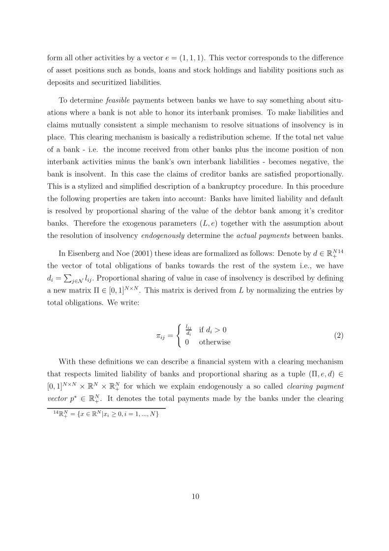
form all other activities by a vector e = (1, 1, 1). This vector corresponds to the difference

of asset positions such as bonds, loans and stock holdings and liability positions such as

deposits and securitized liabilities.

To determine feasible payments between banks we have to say something about situ-

ations where a bank is not able to honor its interbank promises. To make liabilities and

claims mutually consistent a simple mechanism to resolve situations of insolvency is in

place. This clearing mechanism is basically a redistribution scheme. If the total net value

of a bank - i.e. the income received from other banks plus the income position of non

interbank activities minus the bank’s own interbank liabilities - becomes negative, the

bank is insolvent. In this case the claims of creditor banks are satisfied proportionally.

This is a stylized and simplified description of a bankruptcy procedure. In this procedure

the following properties are taken into account: Banks have limited liability and default

is resolved by proportional sharing of the value of the debtor bank among it’s creditor

banks. Therefore the exogenous parameters (L, e) together with the assumption about

the resolution of insolvency endogenously determine the actual payments between banks.

In Eisenberg and Noe (2001) these ideas are formalized as follows: Denote by d ∈ RN+

14

the vector of total obligations of banks towards the rest of the system i.e., we have

di =∑

j∈N lij. Proportional sharing of value in case of insolvency is described by defining

a new matrix Π ∈ [0, 1]N×N . This matrix is derived from L by normalizing the entries by

total obligations. We write:

πij =

{

lij

diif di > 0

0 otherwise(2)

With these definitions we can describe a financial system with a clearing mechanism

that respects limited liability of banks and proportional sharing as a tuple (Π, e, d) ∈

[0, 1]N×N × RN × R

N+ for which we explain endogenously a so called clearing payment

vector p∗ ∈ RN+ . It denotes the total payments made by the banks under the clearing

14R

N+ = {x ∈ R

N |xi ≥ 0, i = 1, ..., N}

10

mechanism. We have:

Definition 1 A clearing payment vector for the system (Π, e, d) ∈ [0, 1]N×N × RN × R

N+

is a vector p∗ ∈ ×Ni=1[0, d

i] such that for all i ∈ N

p∗i = min[di, max(N

∑

j=1

πjip∗j + ei, 0)] (3)

Applied to our example the normalized liability matrix is given by

Π =

0 0 13

40 1

4

3

4

1

40

For an arbitrary vector of actual payments p between banks the net values of banks

can then be written as

ΠT p + e − p

Under the clearing mechanism - given the payments of all counterparties in the inter-

bank market - a bank either honors all it’s promises and pays p∗i = di or it is insolvent

and pays

p∗i = max(

N∑

j=1

πjip∗j + ei, 0) (4)

The clearing payment vector thus directly gives us two important insights. First: For a

given structure of liabilities and bank values (Π, e, d) it tells us which banks in the system

are insolvent. Second: It tells us the recovery rate for each defaulting bank in each state.

To find a clearing payment vector we have to find a solution to a system of inequalities.

Eisenberg and Noe (2001) prove that under mild regularity conditions a unique clearing

payment vector for (Π, e, d) always exists. These results extend - with slight modifications

- to our framework as well.15

The clearing algorithm contains even more information that is interesting for the

assessment of credit risk in the interbank market and for issues of systemic stability. This

can be seen by an explanation of the method by which we calculate clearing payment

15In Eisenberg and Noe (2001) the vector e is in RN+ whereas in our case the vector is in R

N .

11

vectors. This method is due to Eisenberg and Noe (2001). They call their procedure

the ”fictitious default algorithm”. This term basically describes what is going on in the

calculation. For a given (Π, e, d) the procedure starts under the assumption that all banks

fully honor their promises, i.e. p∗ = d. If under this assumption all banks have positive

value, the procedure stops. If there are banks with a negative value, they are declared

insolvent and the clearing mechanism calculates their payment according to the clearing

formula (4) and keeps the payments of the positive value banks fixed. Now it can happen

that banks that had a positive value in the first iteration have a negative value in the

second because they loose on their claims on the insolvent banks. Then these banks

have to be cleared and a new iteration starts. Eisenberg and Noe (2001) prove that this

procedure is well defined and converges after at most N steps to the unique clearing

payment vector p∗.16

This procedure thus generates interesting information in the light of systemic stability.

A bank that is insolvent in the first round of the fictitious default algorithm is fundamen-

tally insolvent. Bank defaults in consecutive rounds can be considered as contagious

defaults.17

An application of the fictitious default algorithm to our example leads to a clearing

payment vector of p∗ = (2, 28

15, 52

15). It is easy to check that bank 2 is fundamentally

insolvent whereas bank 3 is “dragged into insolvency“ by the default of bank 2.

To extend the model of the clearing system to a simple uncertainty framework we

work with a basic event tree. Assume that there are two dates t = 0 and t = 1. Think of

16Note that our setup implicitly contains a seniority structure of different debt claims of banks. Byinterpreting ei as net income from all bank activities except the interbank business we assume thatinterbank debt claims are junior to other claims, like depositors or bond holders. However interbankclaims have absolute priority in the sense that the owners of the bank get paid only after all debts havebeen paid. In reality the legal situation is much more complicated and the seniority structure mightvery well differ from the simple procedure we employ here. For our purpose it gives us a convenientsimplification that makes a rigorous analysis of interbank defaults tractable.

17At this point is is perhaps useful to point out that the clearing payment vector is a fixed pointof the map ×N

i=1[0, di] → ×Ni=1[0, di], p 7→ ((ΠT p + e − p) ∨ 0) ∧ d whereas the dynamic interpretation

is derived from the iterative procedure by which the fixed point is actually calculated. We thereforehesitate to follow Eisenberg and Noe (2001) by interpreting insolvencies at later rounds of the fictitiousdefault algorithm as indicating higher “systemic stability“ of a bank. Of course one can define such ameasure. Since there are other ways to calculate the clearing payment vector, the order of rounds in thefictitious default algorithm does not have a meaningful economic interpretation. The fictitious defaultalgorithm nevertheless allows for a meaningful decomposition between defaults directly due to shocks orindirectly due to default of other banks in the system. No matter how the clearing vector is calculatedthe interpretation of fundamental insolvency has a clear economic interpretation and the classification ofall other defaults as contagious does not depend on the particular calculation procedure, i.e. the fictitiousdefault algorithm.

12

�

� �

������� ��� � ���� �������� ��� � ���

������������ � � �

��

���� �

�� � ���� �

��� ��� !#" ��� ��� !%$

�

� �

�������&��� � ���� ��������&��� � ���

��������&��� � � �

�

�

� � �

Figure 2. Graphical representation of the simple toy-model network of interbank liabilities.

t = 0 as the observation period, where (L, e0) is observed. Then economic shocks affect

the income vector e0. The shocks lead to a realization of one state s in a finite set S

of states of the world at t = 1. Each state is characterized by a particular es1. Think

of t = 1 as a hypothetical clearing date where all interbank claims are settled according

to the clearing mechanism. By the theorem of Eisenberg and Noe (2001) we know that

such a clearing payment vector is uniquely determined for each pair (L, es1). Thus from

an ex-ante perspective we can assess expected default frequencies from interbank credits

across states as well as the expected severity of losses from these defaults given we have

an idea about (L, es1) for all s ∈ S. We can furthermore decompose insolvencies across

states into fundamental and contagious defaults.

Going back to our example we could think of a situation with two states described by

two vectors e11 = (1, 1, 1) and e21 = (1, 3, 2). Given in the observation period we have

seen the matrix L, in the first state banks 2 and 3 default whereas in the second state

no bank is insolvent. The clearing payment vectors and the network structure for this

example are illustrated in Figure 2.

An application of the network model for the assessment of credit risk from interbank

positions therefore requires mainly two things. First, we have to determine L from the

data. Second, we have to come up with a plausible framework to create meaningful

13

scenarios or states of the world.

3 The Data

In the following we give a short description of our data. Our main sources are bank balance

sheet and supervisory data from the Monatsausweis (MAUS) database of the Austrian

Central Bank (OeNB) and the database of the OeNB major loans register (Großkreditev-

idenz,GKE). We use furthermore data on default frequencies in certain industry groups

from the Austrian rating agency Kreditschutzverband von 1870. Finally we use market

data from Datastream.

3.1 The Bank Balance Sheet Data

Banks in Austria report balance sheet data to the central bank on a monthly basis18. On

top of balance sheet data MAUS contains a fairly extensive amount of other data that

are relevant for supervisory purposes. They include among others numbers on capital

adequacy statistics on times to maturity and foreign exchange exposures with respect to

different currencies. We can use this information to learn more about the structure of

certain balance sheet positions.

In our analysis we use a cross section from the MAUS database for September 2001

which we take as our observation period. We want to use these data to get an estimate

of the matrix L as well as to determine the vector e0. All items are broken down in Euro

exposures and into foreign exchange exposures.

A particular institutional feature of the Austrian banking system helps us with the

estimation of bilateral interbank exposures. It has a sectoral organization for historic

reasons. Banks belong to one of the seven sectors: joint stock banks, savings banks,state

mortgage banks, Raiffeisen banks, Volksbanken, housing construction savings and loan

associations and special purpose banks. This sectoral organization of banks left traces in

the data requirements of OeNB. Banks have to break down their MAUS reports on claims

and liabilities with other banks according to the different banking sectors, central bank

and foreigners. This practice of reporting on balance interbank positions reveals some

18This report called Monatsausweis (MAUS) is regulated in §74 Abs. 1 and 4 of the Austrian bankinglaw, Bankwesengesetz (BWG).

14

structure of the L matrix. The savings banks and the Volksbanken sector are organized

in a two tier structure with a sectoral head institution. The Raiffeisen sector is organized

by a three tier structure, with a head institution for every federal state of Austria. The

federal state head institutions have a central institution, Raiffeisenzentralbank (RZB)

which is at the top of the Raiffeisen structure. Banks with a head institution have to

disclose their positions with the head institution. This gives us additional information

on L. From the viewpoint of banking activities the sectoral organization is today not

particularly relevant. The activities of the sectors differ only slightly and only a few

banks are specialized in specific lines of business. The 908 independent banks in our

sample are to the largest extent universal banks.

Total assets in the Austrian banking sector in September 2001 were 567, 071 Million

Euro. The sectoral shares are: 22% joint stock banks, 35% savings banks, 6% state

mortgage banks, 21% Raiffeisen banks, 5% Volksbanken, 3% housing construction savings

and loan associations and 8% special purpose banks. The banking system is dominated

by a few big institutions: 57% of total assets are concentrated with the 10 biggest banks.

The share of total interbank liabilities in total assets of the banking system is 33%.

Statistics for the data on domestic interbank exposures are displayed in Table 1, which

shows sectoral aggregates of the domestic on balance sheet exposures for the Austrian

interbank market. About two thirds of all Austrian banks belong to the Raiffeisen sector

which consists mainly of small, independent banks in rural areas. From the fraction of

liabilities in the won sector we can see that some sectors form a fairly closed system

holding about three quarters of the liabilities within the sector, while the construction

S&Ls have no liabilities to banks in their sector. We can also see that banks in a sector

with a head institution do the major share of their interbank activities with their own

head institution. This is in particular true for many of the smaller banks. The special

purpose banks are quite diversified in their liabilities.

3.2 The Credit Exposure Data

We can get a rough breakdown for the banks’ loan portfolio to non-banks by making use

of the major loans register of OeNB (Großkreditevidenz, GKE). This database contains

all loans exceeding a volume of 364, 000 Euro. For each bank we use the amount of loans

15

Jointstockbanks

Savingsbanks

Statemortgage

banks

Raiffeisenbanks

Volks-banken

Construc-tionS&Ls

Specialpurpose

banks

Number of banks 61 67 8 617 71 5 79

Fraction ofliabilities in ownsector

74% 35% 10% 75% 73% 0% 7%

Exposure to centralinstitution as shareof total exposure

- 60% - 77% 71% - -

Exposure to centralinstitution as shareof sector exposure

- 79% - 88% 89% -

Joint stock banks 9291.8510 606.4400 77.4930 438.1340 123.3800 15.1310 1929.6130Savings banks 9176.8560 6201.8740 208.2580 326.1450 55.2190 3.2040 1636.9970State Mortgage b. 269.5640 61.2650 76.9350 110.2090 8.4670 4.9470 265.5170Raiffeisen banks 761.8140 265.9590 121.1780

15166.387035.2130 692.4990 3313.8260

Volksbanken 467.2920 10.0400 58.9800 313.3170 2848.4250 21.4760 205.5010Construction S&Ls 0.0000 22.7740 0.0000 222.2600 0.0000 0.0000 34.4030Special purpose b. 2044.3760 1083.3340 131.7620 660.3960 93.4950 0.0020 278.1220

Table 1. Sectoral decomposition of interbank liabilities. The table shows the number of banksin each sector, the average fraction of interbank liabilities towards banks in the own sector asshare of total exposure, the average fraction of interbank liabilities towards banks in the ownsector as share of their sector exposure as well as the average liability of sectorally organizedbanks with their head institution. The first row in the lower block shows liabilities of joint stockbanks against joint stock banks, of joint stock banks against savings banks etc.. The next rowis to be read in the same way. These numbers are in Million Euro.

to enterprises from 35 sectors classified according to the NACE standard.19 It gives us the

volume as well as the number of credits to these different industry branches. Combining

this information with data from the Austrian Rating Agency Kreditschutzverband von

1870 (KSV) we can estimate the riskiness of a loan in a certain industry. The KSV

database gives us time series of default rates for the different NACE branches. From this

statistics we can produce an average default frequency and its standard deviation for each

NACE branch. These data serve as our input to the credit risk model.20

19We use the classification according to ONACE 1995. This is the Austrian version of NACE Rev. 1, a European classification scheme, which has to be applied according to VO (EWG) Nr. 3037/ 90 forall member states. NACE is an acronym for Nomenclature generale des activites economiques dans lescommunautes europeennes.

20The matching procedure we apply suffers from some data inconsistencies. Though the data come inprinciple from the same sources the reporting procedures are not rooted in exactly the same legal base.So there might be discrepancies in the numbers. MAUS is legally based on the Austrian law on banking,Bankwesengesetz (BWG) whereas the legal base for GKE is the BWG plus a special regulation for loans

16

For the part of loans we can not allocate to industry sectors we have no default

statistics and no numbers of loans. To construct an insolvency statistics for the residual

sector we take averages from the data that are available. To construct a number of loans

figure for the residual sector we assume the share of loan numbers in industry and in

the residual sector is proportional to the share of loan volume between these sectors. We

have chosen this approach for a lack of better alternatives. We should also note that

the insolvency series is very short. The series are available semi-annually beginning with

January 1997 which gives us 8 observations per sector. Thus the estimate of mean default

rates and their standard deviation we can get from these data is noisy.21 We display

average default frequencies and their standard deviation that we get from these data in

Table 10 in Appendix A.

3.3 Market Data

Some positions on the banks’ asset portfolios are subject to market risk. We collect market

data corresponding to the exposure categories over twelve years from September 1989 to

September 2001 from Datastream. These data are used for the creation of scenarios.

Specifically we collect exchange rates of USD, JPY, GBP and CHF to the Austrian

Schilling (Euro) to compute exchange rate risk. As we only have data on domestic and

international equity exposure we include the Austrian index ATX and the MSCI-world

index in our analysis. To account for interest rate risk, we compute zero bond prices for

three month, one, five and ten years, from collected zero rates for EUR, USD, JPY, GBP

and CHF.22

with volume above a certain threshold (Großkreditmeldungsverordnung GKMVO).21In particular the data don’t contain a business cycle. Again we have to live with this short series

because this is the most we can get at the moment. These estimates will become better in the futurehowever as more observations are collected.

22Sometimes a zero bond series is not available for the length of the period we need for our exercise.In these cases we took swap rates.

17

4 Estimating Interbank Liabilities from Partial In-

formation

If we want to apply the network model to our data we have the problem that they contain

only partial information about the interbank liability matrix L. The bank by bank record

of assets and liabilities with other banks gives us the column and row sums of the matrix

L. Furthermore we know some structural information. For instance we know that the

diagonal of L (and thus of Π) must contain only zeros since banks do not have claims and

liabilities against themselves.

The sectoral structure of the Austrian banking system gives us additional information

we can exploit for the reconstruction of the L matrix. The bank records contain claims

and liabilities against the different sectors. Hence we know the column and row sums of

the submatrices of the sectors. Two sectors have a two tier and one sector has a three

tier structure. Banks in these sectors break down their reports further according to the

amount they hold with the central institution. Due to the fact that there are many banks

that hold all their claims and liabilities within their sector or only against the respective

central institution these pieces of information determine already 72% of all entries of the

matrix L exactly. Therefore by exploiting the sectoral information, we actually know a

major part of L from our data.

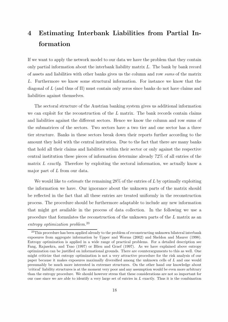
We would like to estimate the remaining 28% of the entries of L by optimally exploiting

the information we have. Our ignorance about the unknown parts of the matrix should

be reflected in the fact that all these entries are treated uniformly in the reconstruction

process. The procedure should be furthermore adaptable to include any new information

that might get available in the process of data collection. In the following we use a

procedure that formulates the reconstruction of the unknown parts of the L matrix as an

entropy optimization problem.23

23This procedure has been applied already to the problem of reconstructing unknown bilateral interbankexposures from aggregate information by Upper and Worms (2002) and Sheldon and Maurer (1998).Entropy optimization is applied in a wide range of practical problems. For a detailed description seeFang, Rajasekra, and Tsao (1997) or Blien and Graef (1997). As we have explained above entropyoptimization can be justified on informational grounds. There are counterarguments to this as well. Onemight criticize that entropy optimization is not a very attractive procedure for the risk analysis of ourpaper because it makes exposures maximally diversified among the unknown cells of L and one wouldpresumably be much more interested in extremer structures. On the other hand our knowledge about’critical’ liability structures is at the moment very poor and any assumption would be even more arbitrarythan the entropy procedure. We should however stress that these considerations are not so important forour case since we are able to identify a very large set of entries in L exactly. Thus it is the combination

18

What this procedure does can intuitively be explained as follows: It finds a matrix that

fulfills all the constraints we know of and treats all other parts of the matrix as balanced

as possible. This can be formulated as minimizing a suitable measure of distance between

the estimated matrix and a matrix that reflects our a priori knowledge on large parts of

bilateral exposures. It turns out that the so called cross entropy measure is a suitable

concept for this task (see Fang, Rajasekra, and Tsao (1997) or Blien and Graef (1997)).

Assume we have in total K constraints that include all constraints on row and column

sums as well as on the value of particular entries. Let us write these constraints as

N∑

i=1

N∑

j=1

akijlij = bk (5)

for k = 1, ..., K and akij ∈ {0, 1}.

We want to find the matrix L that has the least discrepancy to some a priori matrix

U with respect to the (generalized) cross entropy measure

C(L, U) =

N∑

i=1

N∑

j=1

lij ln(lij

uij

) (6)

among all the matrices fulfilling (5) with the convention that lij = 0 whenever uij = 0

and 0 ln(0

0) is defined to be 0.

Due to data inconsistencies the application of entropy optimization is not straight-

forward. For instance the liabilities of all banks in sector k against all banks in sector l

do typically not equal the claims of all banks in sector l against all banks in sector k.24

We solve this problem by using constructing a start matrix for the entropy maximiza-

tion, which reflects all our a priory knowledge. The procedure is described in detail in

Appendix B

We see three main advantages of this method to deal with the incomplete information

problem raised by our data. First the method is able to include all kinds of constraints

we might find out about the matrix L maybe from different sources. Second, as more

information becomes available the approximation can be improved. Third, there exist

computational procedures that are easy to implement and that can deal efficiently with

of structural knowledge plus entropy optimization which gives the estimation of bilateral exposures somebite.

24We do not know the reasons for these discrepancies. Some of the inconsistencies seem to suggest thatthe banks assign some of their counterparties to the wrong sectors.

19

very large problems (see Fang, Rajasekra, and Tsao (1997) or Blien and Graef (1997)).

Thus problems similar to ours can be solved efficiently and quickly on an ordinary personal

computer, even for very large banking systems.

5 Creating Scenarios

Our model of the banking sector uses different states of the world or scenarios to model

uncertainty. In each scenario banks face gains and losses due to market risk and credit

risk. Some banks may fail which possibly causes subsequent failures of other banks, as

it is modeled in our network clearing framework. In our approach the credit risk in the

interbank network is modeled endogenously while all other risks - like gains and losses

from FX and interest rate changes as well as from equity price changes losses from loans

to non-banks - are reflected in the position ei. The perspective taken in our analysis is to

ask, what are the consequences of different scenarios for ei on the whole banking system.

We choose a standard risk management framework to model the shocks to banks. To

simulate scenario losses that are due to exposures to market risk we conduct a historical

simulation and to capture losses from loans to non-banks we use a credit risk model.

Table 2 shows, which balance sheet items are included in our analysis and how the

risk exposure is modeled. Market risk (stock price changes, interest rate movements and

FX rate shifts) are captured by a historical simulation approach (HS) for all items except

other assets and other liabilities, which includes long term major equity stakes in not-

listed companies, non financial assets like property and IT-equipment and cash on the

asset side and equity capital and provisions on the liability side. Credit losses from non-

banks are modeled via a credit risk model. The credit risk from bonds is not included

since most banks hold only government bonds. The credit risk in the inter-bank market

is determined endogenously.

5.1 Market Risk: Historical Simulation

We use a historical simulation approach as it is documented in the standard risk man-

agement literature (Jorion (2000)) to assess the market risk of the banks in our system.

This methodology has the advantage that we do not have to specify a certain parametric

20

Interest rate/ Credit risk FX riskAssets stock price riskshort term governmentbonds and receivables Yes (HS) No Yes (HS)loans to other banks Yes (HS) endogenous by clearing Yes (HS)loans to non banks Yes (HS) credit risk model Yes (HS)bonds Yes (HS) no as mostly government Yes (HS)stock holdings Yes (HS) No Yes (HS)other assets No No NoLiabilities

liabilities other banks Yes (HS) endogenous by clearing Yes (HS)liabilities non banks Yes (HS) No Yes (HS)securitized liabilities Yes (HS) No Yes (HS)other liabilities No No No

Table 2. The table shows how risk of the different balance sheet positions is covered in ourscenarios. HS is a shortcut for historic simulation.

distribution for our returns. Instead we can use the empirical distribution of past observed

returns and thus capture also extreme changes in market risk factors. From the return

series we draw random dates. By this procedure we capture the joint distribution of

the market risk factors and thus take correlation structures between interest rates, stock

markets and FX markets into account.

To estimate shocks on bank capital stemming from market risk, we include positions in

foreign currency, equity and interest rate sensitive instruments. For each bank we collect

foreign exchange exposures for USD, JPY, GBP and CHF only as no bank in our sample

has open positions of more than 1% of total assets in any other currency. From the MAUS

database we get exposures to foreign and domestic stocks, which is equal to the market

value of the net position held in these categories. The exposure to interest rate risk

can not be read directly from the banks’ monthly reports. We have information on net

positions in all currencies combined for different maturity buckets (up to 3 month but not

callable, 3 month to 1 year, 1 to 5 years, more than 5 years). These given maturity bands

allow only a quite coarse assessment of interest rate risk.25 Nevertheless the available data

25We would like to have a finer granularity in the buckets, because right now a wide range of maturitiesis grouped together. We would prefer more buckets especially in the longer maturities. As the maturitybuckets in the banks’ exposure reports are quite broad, there will be instruments of different maturitiesin each bucket. As we consider only the net position within each bucket for our risk analysis, we mighthave some undesired netting effects that will result in an underestimation of market risk. Consider forexample a five year loan that is financed by one year deposits. As both assets fall into the same bucket,

21

allow us to estimate the impact of changes in the term structure of interest rates. To get

an interest rate exposure for each of the five currencies EUR, USD, JPY, GBP and CHF

we split the aggregate exposure according to the relative weight of foreign currency assets

in total assets. This procedure gives us a vector of 26 exposures, 4 FX, 2 equity, and 20

interest rate, for each bank. Thus we get a N × 26 matrix of market risk exposure.

We collect daily market prices over 3, 219 trading days for the risk factors as described

in subsection 3.3. From the daily prices of the 26 risk factors we compute daily returns. We

rescale these to monthly returns assuming twenty trading days and construct a 26× 3219

matrix R of monthly returns.

For the historical simulation we draw 10, 000 scenarios from the empirical distribution

of returns. To illustrate the procedure let Rs be one such scenario, i.e. a column vector

from the matrix R. Then the profits and losses that arise from a change in the risk factors

as specified by the scenario are simply given by multiplying them with the respective

exposures. Let the exposures that are directly affected by the risk factors in the historical

simulation be denoted by a. The vector aRs contains then the profits or losses each bank

realizes under the scenario s ∈ S. Repeating the procedure for all 10000 scenarios, we get

a distribution of profits and losses due to market risk.

5.2 Credit Risk: Calculating Loan Loss Distributions

For the modeling of loan losses we can not apply a historical simulation as there are

no published time series data on loan defaults. We employ one of the standard modern

credit risk models - CreditRisk+ - to estimate a loan loss distribution for each bank in

our sample.26 We rely on this estimated loss distribution to create for each bank the

loan losses across scenarios. While CreditRisk+ is designed to deal with a single loan

portfolio we have to deal with a system of portfolios since we have to consider all banks

simultaneously. The adaptation of the model to deal with such a system of loan portfolios

turns out to be straightforward.

The basic inputs CreditRisk+ needs to calculate a loss distribution is a set of loan

the net exposure is zero despite of the fact that there is some obvious interest rate risk. We compensatefor this effect by choosing as risk factors for each bucket a zero bond with a maturity at the upper boundof the respective maturity band.

26A recent overview on different standard approaches to model credit risk is Crouhy, Galai, and Mark(2000). CreditRisk+ is a trademark of Credit Suisse Financial Products (CSFP). It is described in detailin CSFP Credit Suisse (1997)

22

exposure data, the average number of defaults in the loan portfolio of the bank and its

standard deviation. Aggregate shocks are captured by estimating a distribution for the

average number of loan defaults for each bank.27 This models business cycle effects on

average industry defaults. The idea is that these default frequencies increase in a re-

cession and decrease in booms. Given this common shock, defaults are assumed to be

conditionally independent. We construct the bank loan portfolios by decomposing the

bank balance sheet information on loans to non banks into volume and number of loans

in different industry sectors according to the information from the major loan register.

The rest is summarized in a residual position as described in Section 3. Using the KSV

insolvency statistics for each of the 35 industry branches and the proxy insolvency statis-

tics for the residual sector, we can assign an average default frequency and a standard

deviation of this frequency to the different industry sectors. The riskiness of a loan in a

particular industry is then assumed to be described by these parameters. Based on this

information we can calculate the average default frequency and it’s standard deviation

for each individual bank portfolio. From these data we then construct the distribution of

the aggregate shock (i.e. the average default frequency of the bank portfolio), for each

bank in our sample.

With these data we are now ready to create loan loss scenarios. First we draw for each

bank a realization from each bank’s individual distribution of average default frequencies.

To model this as an economy wide shock, we draw the same quantile for all banks in

the banking system. Given the average default frequency, defaults are assumed to be

conditionally independent. We can then calculate a conditional loss distribution for each

bank, from which we then draw loan losses.28 In Figure 3 we show an arbitrary bank

form our sample and draw the gamma distribution of average default frequencies for this

bank’s loan portfolio as well as its conditional loss distribution for a default frequency

from the 10%, 50% and 90% quantile realization of the economy wide shock.

27In CreditRisk+ this distribution is specified as a gamma distribution. The parameters of the gammadistribution can be determined by the average number of defaults in the loan portfolio and its standarddeviation.

28To reduce the variance in our Monte Carlo simulation, we go through the quantiles of the distributionof average default frequencies at a step length of 0.01. Thus, we draw hundred economy wide shocks fromeach of which we draw 100 loan loss scenarios, yielding a total number of 10,000 scenarios.

23

0 20 40 60 80 100 120 140 160 180 2000

0.005

0.01

0.015

0.02

0.025

0 1 2 3 4 5 6 7 8 9 100

0.05

0.1

0.15

0.2

0.25

0.3

0.35

0.4

0.45

0.5 ������������� ��������� ������������������ "!# ��$%$%�%��&(')����& *��+��& ,�-.�/10�032546087:9�46;=<>7:46/1?

@�ACB �C����-C��& � �D����

E�ACB �C����-C��& � ������

F�A+B �C�G�-C��& � �����H

Figure 3. Distribution of average default frequency (upper right corner) and corresponding lossdistributions. To model the macroeconomic shock, the same quantile from each bank’s averagedefault frequency distribution is drawn. Depending on this draw, the bank’s loss distributioncan be calculated. Three loss distributions corresponding to the 10%, 50% and 90% quantile ofthe average default frequency distribution for a specific bank are shown.

5.3 Combining Market Risk, Credit Risk, and the Network

Model

The credit losses across scenarios are combined with the results of the historic simulations

to create the total scenarios for es for each bank. By the network model the interbank

payments for each scenario are then endogenously explained by the model for any given

realization of es (see Figure 1). Thus we get endogenously a distribution of clearing

vectors, default frequencies, recovery rates and a statistics on the decomposition into

fundamental and contagious defaults.

24

Minimum 10% Quantile Median 90%Quantile Maximum

Joint stock banks 0% 0% 0.02% 3.70% 69.00%Savings banks 0% 0.01% 0.27% 2.80% 7.43%State Mortgage banks 0% 0.01% 0.42% 2.16% 2.64%Raiffeisen banks 0% 0.01% 0.97% 13.50% 72.57%Volksbanken 0% 0.01% 0.33% 7.19% 84.75%Construction S&Ls 0.09% 0.088% 6.05% 13.46% 13.46%Special purpose banks 0% 0% 0% 0.69% 34.61%

Entire banking system 0% 0% 0.51% 10.68% 84.75%

Table 3. Default probabilities of individual banks, grouped by sectors and for the entire bankingsystem.

6 Results

6.1 Default frequencies

From the network model we get a distribution of clearing vectors p∗ and therefore also

a distribution of insolvencies for each individual bank across states of the world. This

is because whenever a component in p∗ is smaller than the corresponding component in

d the bank has not been able to honor it’s interbank promises. We can thus generate a

distribution of default frequencies for individual sectors and for the banking system as

a whole. The relative frequency of default across states is then interpreted as a default

probability. The distribution of default probabilities is described in Table 3. It shows

minimum, maximum the 10 and 90 percent quantiles as well as the median of individual

bank default probabilities grouped by sectors and for the entire banking system.

We can see from the table that some banks are extremely safe as default probabilities

in the 10 percent quantile are very low and often even zero. Also the median default

probability is below 1 percent for every sector except the Construction S&Ls. Default

probabilities increase as we go to the 90% quantile but they stay fairly low. Very few

banks however have a very high probability of default. For a supervisor, running this

model such banks could be identified from our calculations and looked at more closely to

get a more precise idea, of what the problem might be.

25

Minimum 10% Quantile Median 90%Quantile Maximum

Joint stock banks 0% 0% 51.00% 94.96% 99.70%Savings banks 0% 11.00% 70.57% 90.15% 98.69%State Mortgage banks 0.74% 2.63% 59.45% 93.99% 95.56%Raiffeisen banks 0% 0.75% 65.42% 93.49% 99.22%Volksbanken 0% 7.23% 73.80% 91.26% 96.82%Construction S&Ls 0% 0% 0.37% 48.76% 48.76%Special purpose banks 0% 0% 8.66% 97.70% 98.30%

Entire banking system 0% 0% 65.97% 93.49% 99.70%

Table 4. Individual bank recovery rates of interbank credits grouped by sectors and for theentire banking system.

6.2 Severity of losses: Recovery rates

For the severity of a crises of course default frequencies are not the only thing that counts.

We also want to judge the severity of losses. An advantage of the network model is that

it yields for each bank endogenous recovery rates, i.e. the fraction of actual payments

relative to promised payments in the case of default.29 Of course these recovery rates

must not be taken literally because they are generated by the clearing mechanism of the

model under very specific assumptions. If in reality a bank would become insolvent and

sent into bankruptcy, bankruptcy costs or other sharing rules than assumed in this paper

could affect recovery rates. However the network model can give a good impression on

the order of magnitudes that might be available in such an event. We report expected

recovery ratios in Table 4.

As we can see, the median recovery rate in the banking system is 66 %. Thus for more

than half of the banks in the entire banking system the value of their interbank claims is

not reduced by more than a third in case of default of a counterparty. If we look at the

sectoral grouping of the median recovery rate we see that in the savings bank sector we

have a rate of 90%. The recovery rate for the Construction S&Ls is low.

6.3 Systemic stability: Fundamental versus Contagious Defaults

Let us now turn to the decomposition into fundamental and contagious defaults. This

decomposition is particularly interesting from the viewpoint of systemic stability. It is

also interesting to get an idea about contagion of bank defaults from a real dataset since

29In terms of the network model, it is the ratiop∗

i

di

∀i ∈ N with 0 ≤ p∗i ≤ di.

26

the empirical importance of domino effects in banking has been controversial in the litera-

ture.30 Bank defaults may be driven by large exposures to market and credit risk or from

an inadequate equity base. Bank defaults may however also be initiated by contagion:

as a consequence of a chain reaction of other bank failures in the system. The fictitious

default algorithm allows us to distinguish these different cases.

Non-contagious bank defaults lead to insolvency in the first round of the fictitious

default algorithm. These defaults are a direct result from shocks to fundamental risk

factors of the banks’ businesses. As the iterations of the algorithm increase other banks

may become insolvent as a result of bank failures elsewhere in the system. These cases

may be classified as contagious defaults. These risks are not visible by a regulatory setup

that focuses on individual banks’ ”soundness”. Table 5 summarizes the probabilities of

fundamental and contagious defaults in our data.

We list the probabilities of 0− 10 banks defaulting fundamentally and the probability

of banks defaulting contagiously as a consequence of this event. The next row shows

similar information for the event that 11 − 20 banks get insolvent and the probability

that other banks default contagiously as a consequence of this etc. What is remarkable

in this table is that the relative importance of contagious default events as compared to

the importance of contagious defaults is relatively low. In fact approximately 94% of

default events are directly due to movements in risk factors whereas 6% can be classified

as contagious.

The number of default cases by its own does not provide a full picture of the effects

of insolvency. It is interesting to look also at the size of institutions that are affected.

Describing bank size by total assets, we see that the average bank affected by fundamental

default holds 0.8% of the assets in the banking system. In the worst case of our scenarios

we find that banks holding 38.9% of the assets in the banking system default fundamen-

tally. Looking at contagious defaults across all scenarios total assets of banks affected

are on average 0.05%, whereas in the worst scenario banks with a share of 36.9% in total

assets are affected. In total we have the numbers 0.9% and 37%. Plotting a histogram

of bank defaults by total assets confirms the picture we get from this statistics. Smaller

banks are more likely to fail than the larger banks as we can see in Figure 4.

Our finding that the risk of contagion is relatively small is in line with findings in

Furfine (1999). Upper and Worms (2002), letting one bank fail at a time, find that, while

30See in particular the detailed discussion in Kaufman (1994).

27

Fundamental Contagious Total

0-10 6.06% 0.02% 6.08%11-20 24.62% 0.12% 24.74%21-30 26.16% 0.22% 26.38%31-40 18.11% 0.28% 18.39%41-50 9.36% 0.40% 9.76%51-60 4.50% 0.50% 5.00%61-70 2.24% 0.27% 2.51%71-80 1.31% 0.42% 1.73%81-90 0.68% 0.48% 1.16%91-100 0.38% 0.38% 0.76%more 0.86% 2.63% 3.49%

Total 94.28% 5.72% 100.00%

Table 5. Probabilities of fundamental and contagious defaults. A fundamental default is dueto the losses arising from exposures to market risk and credit risk to the corporate sector, whilea contagious default is triggered by the default of another bank who cannot fulfill its promisesin the interbank market.

0 50000 100000 150000 200000 2500000

0.1

0.2

0.3

0.4

0.5

0.6

0.7

0.8

0.9

Total Assets

Fre

quen

cy

Figure 4. Histogram of bank defaults by total assets.

28

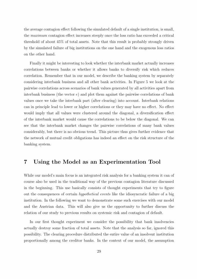
the average contagion effect following the simulated default of a single institution, is small,

the maximum contagion effect increases steeply once the loss ratio has exceeded a critical

threshold of about 45% of total assets. Note that this result is probably strongly driven

by the simulated failure of big institutions on the one hand and the exogenous loss ratios

on the other hand.

Finally it might be interesting to look whether the interbank market actually increases

correlations between banks or whether it allows banks to diversify risk which reduces

correlation. Remember that in our model, we describe the banking system by separately

considering interbank business and all other bank activities. In Figure 5 we look at the

pairwise correlations across scenarios of bank values generated by all activities apart from

interbank business (the vector e) and plot them against the pairwise correlations of bank

values once we take the interbank part (after clearing) into account. Interbank relations

can in principle lead to lower or higher correlations or they may have no effect. No effect

would imply that all values were clustered around the diagonal, a diversification effect

of the interbank market would cause the correlations to be below the diagonal. We can

see that the interbank market changes the pairwise correlations of many bank values

considerably, but there is no obvious trend. This picture thus gives further evidence that

the network of mutual credit obligations has indeed an effect on the risk structure of the

banking system.

7 Using the Model as an Experimentation Tool

While our model’s main focus is an integrated risk analysis for a banking system it can of

course also be used in the traditional way of the previous contagion literature discussed

in the beginning. This use basically consists of thought experiments that try to figure

out the consequences of certain hypothetical events like the idiosyncratic failure of a big

institution. In the following we want to demonstrate some such exercises with our model

and the Austrian data. This will also give us the opportunity to further discuss the

relation of our study to previous results on systemic risk and contagion of default.

In our first thought experiment we consider the possibility that bank insolvencies

actually destroy some fraction of total assets. Note that the analysis so far, ignored this

possibility. The clearing procedure distributed the entire value of an insolvent institution

proportionally among the creditor banks. In the context of our model, the assumption

29

Figure 5. Correlation of bank values with (node values) and without interbank positions (e)across different scenarios.

of zero losses makes sense because the model just tries to assess technical insolvency of

institutions that is implied by the data and the risk analysis. It is not a model that predicts

bankruptcies. Still it might be interesting to ask, what would be the consequences if the

technical insolvencies actually turned out to be true bank breakdowns that destroy asset

values. In line with James (1991) who found that realized losses in bank failures can be

estimated at around 10% of total assets we chose our range of loss rates from 0, 10%, 25%

up to 40% of total assets as our estimate of bankruptcy costs. The results are shown in

Table 6.

Assuming loss rates different from zero percent has little consequences for the ’typical’

scenario. In 77% of the scenarios there are no contagious defaults irrespective of the as-

sumed bankruptcy costs. Yet for some scenarios the consequences can be fairly dramatic.

The maximum number of contagious defaults increases sharply once we assume loss rates

different from zero. For instance at a loss rate of 10% of total assets, the maximum

number of contagious defaults is 413 (45% of all banks) compared to 46 (5%) with a loss

rate of 0%. As we can see, low bankruptcy costs are crucial to systemic stability of the

30

Assumed loss rate 0% 10 % 25% 40 %

Scenarios without Contagious Default 96% 91% 87% 77%Average Number of Contagious Defaults 0.13 1.36 14.06 21.2Maximum Number of Contagious Defaults 46 413 624 629

Table 6. Consequences of different loss rates: The first row displays different assumed loss ratiosas a percentage of total assets. In the second row we see the percentage of scenarios withoutany contagious defaults. The next two rows show the average and the maximum number ofcontagious defaults for the different loss rate assumptions.

Quantiles 90% 95 % 99% 100 %

Fundamental Default 215 472 1732 8527Contagious Default 0 0 6 753

Table 7. Costs of avoiding fundamental and contagious defaults: In the first row we giveestimates for the amount of funds required to avoid fundamental defaults in 90, 95, 99 and 100percent of the scenarios. The second row shows the amounts necessary to avert contagiousdefaults once fundamental defaults have occurred. Costs are in million Euro.

banking system.

Another important issue is the question of how much funds the regulator needs to avoid

fundamental or contagious defaults in each and every scenario. Being slightly less ambi-

tious it could also be interesting to calculate the funds needed for insolvency avoidance

in 90, 95, 99 percent of the scenarios very much in the spirit of a value at risk model. Our

framework can be used for such estimations. As shown in Table 7, a complete avoidance

strategy amounts to about 8.5 billion Euro, which corresponds to 1.5 % of all the assets

held by the banks in the system. By only focusing on avoiding fundamental defaults in

99% of the scenarios the regulator can decrease this amount to about 1.7 billion Euro (or

0.31 % of all total assets). The complete avoidance of contagion - in contrast - has costs

of 753 million Euro (0.13 %) which is comparatively low.

Our analysis so far has assumed that foreign counterparties will always fulfill their

obligations completely. Especially banks which are the most active institutions in the

domestic interbank market have sometimes considerable foreign exposures. To study the

consequences of default of international counterparties we assume that 5, 10, 25 and 40%

of foreign exposures will be lost. We re-run our analysis assuming different loss rate and

record the number of banks that are affected by contagious default in each scenario. Table

8 reports the minimum and the maximum number of banks affected by contagious default

in one scenario as well as quantiles across scenarios.

31

Quantiles of Scenarios Min 25 % 50% 75 % Max

0% loss 0 0 0 0 465% loss 0 2 2 3 5610% loss 2 4 5 6 7825% loss 4 6 7 8 31340% loss 7 13 15 17 472

Table 8. Effects of losses from foreign counterparties: Number of banks that are affectedby contagious default. Each row displays a different assumption on the loss rate on promisedpayments. The columns are the various quantiles of the distribution across scenarios.

Panel A: assumed loss rate 5% of promised payments.Quantiles Min 25 % 50% 75 % Max

Most significant bank 0 0 0 0 72Second most significant bank 0 0 0 0 7510th most significant bank 0 0 1 2 912 most significant banks 0 0 0 1 78

Panel B: assumed loss rate 40% of promised payments.Min 25 % 50% 75 % Max

Most significant bank 1 6 6 7 607Second most significant bank 0 3 5 8 64110th most significant bank 6 54 65 73 5812 most significant banks 6 15 17 20 649

Table 9. Number of contagious defaults following a breakdown of significant institutions, wheresignificance is measured as market share in the domestic interbank market. Quantiles across the10,000 scenarios are shown.

The banking system shows reasonable resilience to losses of 5% and 10%. However

the number of defaults grows dramatically with increasing foreign losses. A scenario plot

is shown in Figure 6. It displays for each scenario, 1 to 10000 the number of contagious

defaults under the assumption that 25% of foreign interbank claims will be lost.

In a similar way as the previous analysis, we can analyze the hypothetical default of

significant institutions in the banking system. This approach has been taken for instance

by Furfine (1999). Following his experiments we calculate the consequences of default of

significant institutions for loss rates of 5% (Table 9, Panel A) and 40% (Table 9, Panel

B). We take the exposure in the interbank market as a measure the significance of an

institution. Table 9 shows that the consequences to the banking system are moderate in

the case where the selected banks are only able to honor 95% of their promised payments

(5% loss). In most scenarios no, or only one bank defaults.

32

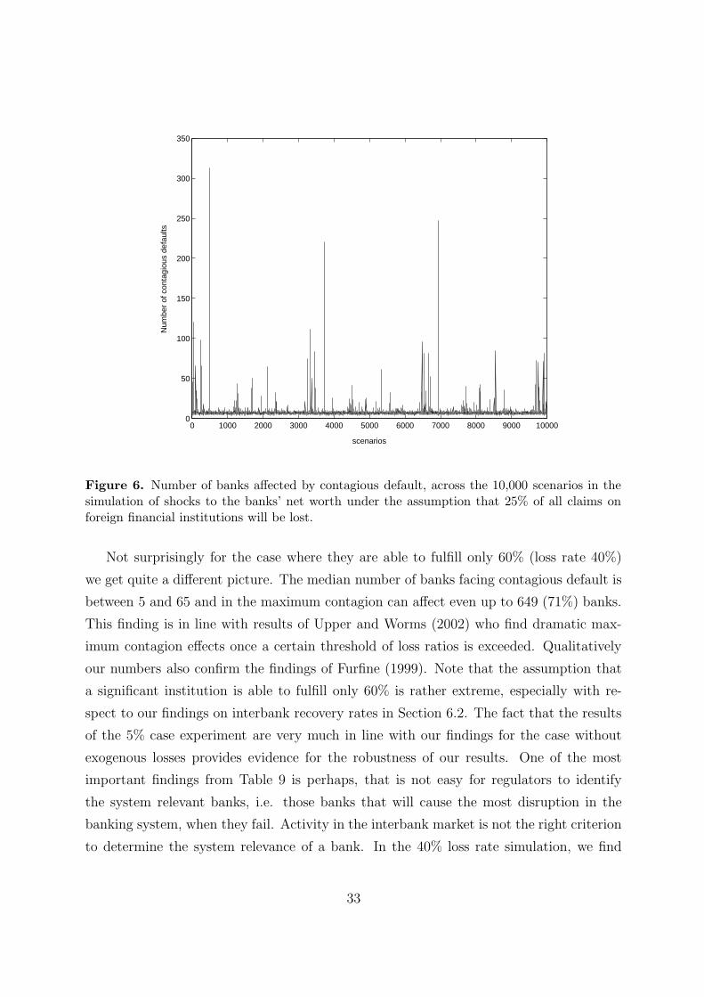
0 1000 2000 3000 4000 5000 6000 7000 8000 9000 100000

50

100

150

200

250

300

350

scenarios

Num

ber

of c

onta

giou

s de

faul

ts

Figure 6. Number of banks affected by contagious default, across the 10,000 scenarios in thesimulation of shocks to the banks’ net worth under the assumption that 25% of all claims onforeign financial institutions will be lost.

Not surprisingly for the case where they are able to fulfill only 60% (loss rate 40%)

we get quite a different picture. The median number of banks facing contagious default is

between 5 and 65 and in the maximum contagion can affect even up to 649 (71%) banks.

This finding is in line with results of Upper and Worms (2002) who find dramatic max-

imum contagion effects once a certain threshold of loss ratios is exceeded. Qualitatively

our numbers also confirm the findings of Furfine (1999). Note that the assumption that

a significant institution is able to fulfill only 60% is rather extreme, especially with re-

spect to our findings on interbank recovery rates in Section 6.2. The fact that the results

of the 5% case experiment are very much in line with our findings for the case without

exogenous losses provides evidence for the robustness of our results. One of the most

important findings from Table 9 is perhaps, that is not easy for regulators to identify

the system relevant banks, i.e. those banks that will cause the most disruption in the

banking system, when they fail. Activity in the interbank market is not the right criterion

to determine the system relevance of a bank. In the 40% loss rate simulation, we find

33

that the medium number of contagious defaults is larger for the tenth most significant

bank than for the first two combined. Again, to identify banks that are a threat financial

stability, supervisors will have to look at the problem from a system perspective and not

at the level of individual banks.

8 Conclusions

In this paper we have developed a new framework for bank risk assessment. The innovation

is that we judge risk at the level of the entire banking system rather than at the level of

an individual institution.

Conceptually it is possible to take this perspective by a systematic analysis of the

impact of a set of macroeconomic risk factors on banks in combination with a network

model of mutual credit relations. Empirically the framework can be applied to real bank-

ing systems because it is designed in such a such a way that it requires data input that is

usually available in one form or another at central banks. This is exactly the institution

for which an assessment method like the one suggested here is of crucial interest. Among

the empirical results we derive for an Austrian dataset perhaps the most interesting is

that contagious default from interbank relations plays only a minor role. It would be

interesting to check the robustness of this empirical result with other observation periods

and with datasets from other countries. We hope to be able to do this in our future

research.

Since our method is a first step, there are certainly many issues that have to be

further discussed to get a firm judgment how much we can trust assessments generated

with the help of our model. We want to point out at this stage, what we see as the main

advantages of our general approach. First the system perspective can uncover exposures

to aggregate risk that are invisible for banking supervision relying on the assessment of

single institutions only. It can furthermore give some idea how to disentangle the risk that

comes from fundamental shocks and the risks that come from contagious bank failures.

As we gain experience with the model for more cases and maybe also for other banking

systems this might create a possibility to qualify the actual importance of contagion effects

that have received so much attention in the theoretical debate. Second we think that our

framework can redirect the discussion about systemic risk in banking from continuous

refinements and extensions of capital adequacy regulation for individual banks to the

34

crucial issue of how much risk is actually borne by the banking system. In this discussion

the framework might be useful to get a clearer picture of actual risk exposure because it

allows for thought experiments. We can relatively easily ask what if questions and with

some further work even develop the framework into a potentially useful stress testing

model. Third the model does not rely on a sophisticated theory of economic behavior. In

fact the model is really a tool to read certain data in a particular way. All it does is to

make the consequences of a given liability and asset structure in combination with realistic

shock scenarios visible in terms of implied technical insolvencies of institutions. We think

that in this context this feature is a definitive advantage because it makes it easier to

validate the model. Fourth the model is designed to exploit existing data sources. Of

course these sources are not ideal because it would be better if we knew more about actual

bilateral exposures and about the important off balance sheet positions. We hope however

that our approach shows that we can start to think about financial stability at the system

level with existing data already. Thus we demonstrate that we do not necessarily have to

wait until reporting systems have been fundamentally reformed. Of course our approach

could perhaps initiate a discussion about such a reform of reporting systems. As we learn

more about the systemic approach to judge risk in the banking system we might get new

ideas about which are the really important pieces of information we need to know for an

analysis of financial stability.

We hope that our ideas will turn out useful for regulators and central bankers by

offering a practicable way to read the data they have at their very doorsteps in the light

of aggregate risk exposure of the banking system. We therefore hope to have given a

perspective of how a ’macroprudential’ approach to banking supervision could proceed.

We also do hope, however, that our paper turns out to be interesting for theoretical work

in financial stability and banking as well and that the questions it raises will contribute in

a fruitful way to the debate about the system approach to banking supervision and risk

assessment.

35

References

Allen, F., and D. Gale, 2000, Financial Contagion, Journal of Political Economy 108,1–34.

Angelini, P., G. Maresca, and D. Russo, 1996, Systemic Risk in the Netting System,Journal of Banking and Finance 20, 853–886.

Blien, U., and F. Graef, 1997, Entropy Optimizing Methods for the Estimation of Tables,in I. Balderjahn, R. Mathar, and M. Schader, eds.: Classification, Data Analysis, andData Highways (Springer Verlag, Berlin ).

Borio, C., 2002, Towards a Macro-Prudential Framework for Financial Supervision andRegulation?, CESifo Lecture, Summer Institute: Banking Regulation and FinancialStability, Venice.

Credit Suisse, 1997, Credit Risk+: A Credit Risk Management Framework. (Credit SuisseFinancial Products).

Crockett, A., 2000, Marrying the Micro- and Macro-Prudential Dimensions of FinancialStability, Speech at the Eleventh International Conference of Banking Supervisors,Basel.

Crouhy, M., D. Galai, and R. Mark, 2000, A comparative analysis of current credit riskmodels, Journal of Banking and Finance 24, 59–117.

Dasgupta, A., 2000, Financial Contagion through Capital Connections: A model of theOrigin and Spread of Bank Panics, mimeo.

Eisenberg, L., and T. Noe, 2001, Systemic Risk in Financial Systems, Management Science47, 236–249.

Fang, S.C., J.R. Rajasekra, and J. Tsao, 1997, Entropy Optimization and MathematicalProgramming. (Kluwer Academic Publishers Boston, London, Dordrecht).

Freixas, X., L. Parigi, and J.C. Rochet, 2000, Systemic Risk, Interbank Relations andLiquidity Provision by the Central Bank, Journal of Money Credit and Banking 32.

Furfine, C., 1999, Interbank Exposures: Quantifying the Risk of Contagion, BIS WorkingPaper, 70.

Hellwig, M., 1995, Systemic Aspects of Risk Management in Banking and Finance,Schweizerische Zeitschrift fuer Volkswirtschaft und Statistik/Swiss Journal of Eco-nomics and Statistics 131, 723–737.

Hellwig, M., 1997, Systemische Risiken im Finanzsektor, in D. Duwendag, eds.:Finanzmarkte im Spannungsfeld von Globalisierung, Regulierung und Geldpolitik(Duncker & Humblot, Berlin ).

36

Humphery, D.B., 1986, Payments Finality and Risk of Settlement Failure, in A.S. Saun-ders, and L.J. White, eds.: Technology and Regulation of Financial Markets: Securities,Futures and Banking (Lexington Books, MA ).

James, C., 1991, The Losses Realized in Bank Failures, Journal of Finance 46, 1223–1242.

Jorion, P., 2000, Value-at-Risk. (McGraw-Hill) second edn.

Kaufman, G., 1994, Bank Contagion: A Review of the Theory and Evidence, Journal ofFinancial Service Research 8, 123–150.

Luenberger, D., 1969, Optimization by Vector Space Methods. (Wiley & Sons).

Sheldon, G., and M. Maurer, 1998, Interbank Lending and Systemic Risk, Swiss Journalof Economics and Statistics 134, 685–704.

Summer, M., 2003, Banking Regulation and Systemic Risk, Open Economies Review,forthcoming.

Upper, C., and A. Worms, 2002, Estimating bilateral exposures in the German Inter-bank Market: Is there a Danger of Contagion?, Deutsche Bundesbank, Dicussion paper09/02.

37

A Data

We use bank balance sheet data from the OeNB MAUS database. The detailed descriptionof these data are available in an extensive manual on the internet at the OeNB website.(See http://www2.oenb.at/rel/melde4 p.htm, item 4.5. ”Positionsnummern”. The dataare a cross section of 908 banks from September 2001. The details of the position numberare described in the OeNB document on the website. The description is only available inGerman. All numbers are in million Euros up to three digits.

The major loan register of OeNB is also described in a manual available form theweb at http://www2.oenb.at/groevi p.htm. The major loans register contains all creditsexceeding a volume of 363364 Euro. Thus some banks are not contained in this sample.Their exposure to the different industry groups is counted as zero and any positive expo-sure they might have is assigned to the difference position as described in the text. 92%of the banks in our sample have positions in the credit exposure statistics. All numbersare in Million Euros up to three digits.

The OeNACE industry categories are formed according to the international NACEnorm. The industry sectors are Agriculture and Fishing; Forestry; Mining and quar-rying of energy producing materials; Manufacture of food products, beverages and to-bacco; Manufacture of textiles and textile products; Manufacture of cloths; Manufactureof leather and leather products; Manufacture of wood and wood products; Manufactureof pulp, paper and paper products; Publishing and printing; Manufacture of chemicals,chemical products and man-made fibers; Manufacture of Rubber and synthetics and plas-tics; Manufacture of basic metals and fabricated metal products; Manufacture of machin-ery and equipment n.e.c.; Manufacture of electrical and optical equipment; Broadcasting;Manufacture of transport equipment; Manufacturing of toys n.e.c.; Electricity, gas andwater supply; Construction; Wholesale and repair of vehicles; Wholesale and retail trade;Hotels and restaurants; Transport, storage and communication; Services for travel; Realestate, renting and business activities; Databases and Data Administration; Research andDevelopment; Enterprise specific services; Education; Health and social services; Recy-cling; Sports and Entertainment; Syndicated loans; Other Services;

We have furthermore for all these industry groups the number of outstanding creditsper bank. This allows us to calculate average exposures.

From the KSV database we have for each industry group described above time seriesof active firms and total number of insolvencies. The observations are on a half yearbase starting from January 1997, reaching to July 2001. This gives us eight observationsper sector. From these observations we calculate average number of defaults and theirstandard deviation. Combining these data with the number of credits in each sector,we can calculate the expected number of default for each bank in each sector. We usefurthermore averages of available data to replace missing observations as well as the datafor the residual position resulting of the difference between total loans per bank and theaggregate exposure from the credit exposure statistics. Average Default frequencies andtheir standard deviation are displays in Table 10.

38

Sector Name µ σ

Agriculture, Fishing, Forestry 0.023 0.015Mining, quarrying of energy producing materials 0.019 0.01Manufacture of food products, beverages and tobacco 0.026 0.004Manufacture of textiles and textile products 0.04 0.01Manufacture of cloths 0.05 0.01Manufacture of leather and leather products 0.04 0.005Manufacture of wood and wood products 0.02 0.002Manufacture of pulp and paper 0.01 0.01Publishing and printing 0.03 0.005Petroleum processing; 0.02 0.01Manufacture of chemicals and man-made fibers 0.02 0.01Manufacture of Rubber and synthetics and plastics 0.03 0.01Manufacture of glass 0.02 0.01Manufacture of basic metals and fabricated metal products 0.03 0.02Manufacture of machinery and equipment 0.03 0.003Manufacture of electrical and optical equipment 0.02 0.005Manufacture of toys and furniture 0.02 0.003Recycling 0.01 0.004Electricity, gas and water supply 0.004 0.004Construction 0.04 0.002Transport, storage and communication; 0.023 0.004Wholesale and retail trade 0.02 0.003Wholesale and repair of vehicles 0.03 0.002Hotels and restaurants; 0.05 0.006Services for travel; 0.04 0.01Broadcasting 0.03 0.01Real estate 0.02 0.005Renting and Business activities 0.03 0.008Holding companies 0.02 0.001Databases 0.02 0.006Education 0.01 0.003Health and Social Services 0.009 0.001Other Services 0.03 0.002Residual Sector 0.03 0.006

Table 10. Estimated average default frequencies µ for GKE sectors and their standard deviationσ.

39

B Inconsistent Constraints for the matrix L

The constraints for the estaimations of the matrix L are not always consistent. Forinstance the liabilities of all banks in sector k against all banks in sector l do typicallynot equal the claims of all banks in sector l against all banks in sector k. We deal withthis problem by applying a two step procedure.

In a first step we replace an a priori matrix U reflecting only possible links betweenbanks by an a priori matrix V that takes actual exposure levels into account. As there areseven sectors we partition V and U into 49 submatrices V kl and Ukl which describe theliabilities of the banks in sector k against the banks in sector l and our a priori knowledge.Given the bank balance sheet data we define uij = 1 if bank i belonging to sector k mighthave liabilities against bank j belonging to sector l and uij = 0 otherwise. The (equality)constraints are that the liabilities of bank i against the sector l equal the row sum of thesubmatrix and that the claims of bank j against the sector k equal the column sum ofthe submatrix, i.e.

∑

j∈l

vij = liabilities of bank i against sector l (7)

∑

i∈k

vij = claims of bank j against sector k (8)

For the matrices describing claims and liabilities within a sector (i.e. V kk) which hasa central institution we get further constraints. Suppose that bank j∗ is the centralinstitution. Then

vij∗ = liabilities of bank i against central institution (9)

vj∗i = claims of bank i against central institution (10)

Though these constraints are inconsistent given our data, we use the information toget a revised matrix V which reflects our a priori knowledge better than the initial matrixU . Contrary to U which consists only of zeroes and ones, the entries in V are adjustedto the actual exposure levels.31

In a second step we recombine the results of the 49 approximations V kl to get an entireN × N improved a priori matrix V of interbank claims and liabilities. Now we replacethe original constraints by just requiring that the sum of all (interbank) liabilities of eachbank equals the row sum of L and the sum of all claims of each bank equals the columnsum of L.

N∑

j=1

lij = liabilities of bank i against all other banks (11)

31Note that the algorithm that calculates the minimum entropy entries does not converge to a solution ifdata are inconsistent. Thus to arrive at the approximation V we terminate after 10 iterations immediatelyafter all row constraints are fulfilled.

40

N∑

i=1

lij = claims of bank j against all other banks (12)

Again we face the problem that the sum of all liabilities does not equal the sum of allclaims but corresponds to only 96% of them. By scaling the claims of each bank by 0.96we enforce consistency.32 Given these constraints and the prior matrix V we estimate thematrix L.

Finally we can use the information on claims and liabilities with the central bankand with banks abroad. By adding two further nodes and by appending the rows andcolumns for these nodes to the L matrix, we get a closed (consistent) system of theinterbank network.

C Approximation of L

To approximate L we solve the problem

minlij

C(L, U) =

N∑

i=1

N∑

j=1

lij ln (lij

uij

)

N∑

i=1

N∑

j=1

akijlij ≤ bk for k = 1, ..., K and akij∈ {0, 1}

lij ≥ 0 for all i, j ∈ N

The Lagrangian for this problem is

L(L, λ, µ) =

N∑

i=1

N∑

j=1

lij ln (lij

uij

)−K

∑

k=1

λk(bk−N

∑

i=1

N∑

j=1

akijlij)−N

∑

i=1

N∑

j=1

µijlij

For this problem the Kuhn-Tucker Conditions (See Luenberger (1969)) can be statedas:

ln (lij

uij

) + 1+

K∑

k=1

λkakij−µij = 0

λk(bk−N

∑

i=1

N∑

j=1

akijlij) = 0 (13)

µijlij = 0

32The remaining 4 % of the claims are added to the vector e. Hence they are assumed to be fulfilledexactly.

41

A computationally efficient method to solve this problem is Bregman’s BalancingProcedure, described in Fang, Rajasekra, and Tsao (1997) and also referred to as entropyprojection method in the literature (Blien and Graef (1997)). In our case we have onlyequality constraints and thus the solution to (13) can be calculated by the RAS algorithmwhich is a special case of the entropy projection method. In our case the constraints aregiven as

N∑

j=1

lij= bri for all i and

N∑

i=1

lij= bcj for all j

In this case an iterative procedure that calculates

lt+1

ij =ltijb

cj

∑

r ltrj

and lt+1

ij =ltijb

rj

∑

c ltrc

solves (13) for any prescribed level of accuracy ε > 0. Convergence of the procedure isshown in (Fang, Rajasekra, and Tsao (1997)).

42

43

Index of Working Papers: August 28, 1990

Pauer Franz

11) Hat Böhm-Bawerk Recht gehabt? Zum Zu-

sammenhang zwischen Handelsbilanzpas-sivum und Budgetdefizit in den USA2)

March 20, 1991

Backé Peter

21)

Ost- und Mitteleuropa auf dem Weg zur Marktwirtschaft - Anpassungskrise 1990

March 14, 1991

Pauer Franz

31)

Die Wirtschaft Österreichs im Vergleich zu den EG-Staaten - eine makroökonomische Analyse für die 80er Jahre

May 28, 1991 Mauler Kurt

41)

The Soviet Banking Reform

July 16, 1991 Pauer Franz

51)

Die Auswirkungen der Finanzmarkt- und Kapitalverkehrsliberalisierung auf die Wirtschaftsentwicklung und Wirtschaftspolitik in Norwegen, Schweden, Finnland und Großbritannien - mögliche Konsequenzen für Österreich3)

August 1, 1991 Backé Peter

61)

Zwei Jahre G-24-Prozess: Bestandsauf-nahme und Perspektiven unter besonderer Berücksichtigung makroökonomischer Unterstützungsleistungen4)

August 8, 1991 Holzmann Robert

71)

Die Finanzoperationen der öffentlichen Haushalte der Reformländer CSFR, Polen und Ungarn: Eine erste quantitative Analyse

January 27, 1992

Pauer Franz

81)

Erfüllung der Konvergenzkriterien durch die EG-Staaten und die EG-Mitgliedswerber Schweden und Österreich5)

October 12, 1992

Hochreiter Eduard (Editor)

91)

Alternative Strategies For Overcoming the Current Output Decline of Economies in Transition

November 10, 1992

Hochreiter Eduard and Winckler Georg

101) Signaling a Hard Currency Strategy: The

Case of Austria

1) vergriffen (out of print) 2) In abgeänderter Form erschienen in Berichte und Studien Nr. 4/1990, S 74 ff 3) In abgeänderter Form erschienen in Berichte und Studien Nr. 4/1991, S 44 ff 4) In abgeänderter Form erschienen in Berichte und Studien Nr. 3/1991, S 39 ff 5) In abgeänderter Form erschienen in Berichte und Studien Nr. 1/1992, S 54 ff

44

March 12, 1993 Hochreiter Eduard (Editor)

11 The Impact of the Opening-up of the East on the Austrian Economy - A First Quantitative Assessment

June 8, 1993 Anulova Guzel 12 The Scope for Regional Autonomy in Russia

July 14, 1993 Mundell Robert 13 EMU and the International Monetary Sy-stem: A Transatlantic Perspective

November 29, 1993

Hochreiter Eduard 14 Austria’s Role as a Bridgehead Between East and West

March 8, 1994 Hochreiter Eduard (Editor)

15 Prospects for Growth in Eastern Europe

June 8, 1994 Mader Richard 16 A Survey of the Austrian Capital Market

September 1, 1994

Andersen Palle and Dittus Peter

17 Trade and Employment: Can We Afford Better Market Access for Eastern Europe?

November 21, 1994

Rautava Jouko 181) Interdependence of Politics and Economic

Development: Financial Stabilization in Russia

January 30, 1995 Hochreiter Eduard (Editor)

19 Austrian Exchange Rate Policy and European Monetary Integration - Selected Issues

October 3, 1995 Groeneveld Hans 20 Monetary Spill-over Effects in the ERM: The Case of Austria, a Former Shadow Member

December 6, 1995

Frydman Roman et al 21 Investing in Insider-dominated Firms: A Study of Voucher Privatization Funds in Russia

March 5, 1996 Wissels Rutger 22 Recovery in Eastern Europe: Pessimism Confounded ?

June 25, 1996 Pauer Franz 23 Will Asymmetric Shocks Pose a Serious Problem in EMU?

September 19, 1997

Koch Elmar B. 24 Exchange Rates and Monetary Policy in Central Europe - a Survey of Some Issues

April 15, 1998 Weber Axel A. 25 Sources of Currency Crises: An Empirical Analysis

45

May 28,1998 Brandner Peter, Diebalek Leopold and Schuberth Helene

26 Structural Budget Deficits and Sustainability of Fiscal Positions in the European Union

June 15, 1998 Canzeroni Matthew, Cumby Robert, Diba Behzad and Eudey Gwen

27 Trends in European Productivity: Implications for Real Exchange Rates, Real Interest Rates and Inflation Differentials

June 20, 1998 MacDonald Ronald 28 What Do We Really Know About Real Exchange Rates?

June 30, 1998 Campa José and Wolf Holger

29 Goods Arbitrage and Real Exchange Rate Stationarity

July 3,1998 Papell David H. 30 The Great Appreciation, the Great Depreciation, and the Purchasing Power Parity Hypothesis

July 20,1998 Chinn Menzie David 31 The Usual Suspects? Productivity and Demand Shocks and Asia-Pacific Real Exchange Rates

July 30,1998 Cecchetti Stephen G., Mark Nelson C., Sonora Robert

32 Price Level Convergence Among United States Cities: Lessons for the European Central Bank

September 30, 1998

Christine Gartner, Gert Wehinger

33 Core Inflation in Selected European Union Countries

November 5, 1998

José Viñals and Juan F. Jimeno

34 The Impact of EMU on European Unemployment

December 11, 1998

Helene Schuberth and Gert Wehinger

35 Room for Manoeuvre of Economic Policy in the EU Countries – Are there Costs of Joining EMU?

December 21, 1998

Dennis C. Mueller and Burkhard Raunig

36 Heterogeneities within Industries and Structure-Performance Models

May 21, 1999 Alois Geyer and Richard Mader

37 Estimation of the Term Structure of Interest Rates – A Parametric Approach

July 29, 1999 José Viñals and Javier Vallés

38 On the Real Effects of Monetary Policy: A Central Banker´s View

December 20, 1999

John R. Freeman, Jude C. Hays and Helmut Stix

39 Democracy and Markets: The Case of Exchange Rates

46

March 01, 2000 Eduard Hochreiter and Tadeusz Kowalski

40 Central Banks in European Emerging Market Economies in the 1990s

March 20, 2000 Katrin Wesche 41 Is there a Credit Channel in Austria? The Impact of Monetary Policy on Firms’ Investment Decisions

June 20, 2000 Jarko Fidrmuc and Jan Fidrmuc

42 Integration, Disintegration and Trade in Europe: Evolution of Trade Relations During the 1990s

March 06, 2001 Marc Flandreau 43 The Bank, the States, and the Market, A Austro-Hungarian Tale for Euroland, 1867-1914

May 01, 2001 Otmar Issing 44 The Euro Area and the Single Monetary Policy

May 18, 2001 Sylvia Kaufmann 45 Is there an asymmetric effect of monetary policy over time? A Bayesian analysis using Austrian data.

May 31, 2001 Paul De Grauwe and Marianna Grimaldi

46 Exchange Rates, Prices and Money. A LongRun Perspective

June 25, 2001 Vítor Gaspar, Gabriel Perez-Quiros and Jorge Sicilia

47 The ECB Monetary Strategy and the Money Market

July 27, 2001 David T. Llewellyn

48 A Regulatory Regime For Financial Stability

August 24, 2001

Helmut Elsinger and Martin Summer

49 Arbitrage Arbitrage and Optimal Portfolio Choice with Financial Constraints

September 1, 2001

Michael D. Goldberg and Roman Frydman

50 Macroeconomic Fundamentals and the DM/$ Exchange Rate: Temporal Instability and the Monetary Model

September 8, 2001

Vittorio Corbo, Oscar Landerretche and Klaus Schmidt-Hebbel

51 Assessing Inflation Targeting after a Decadeof World Experience

September 25, 2001

Kenneth N. Kuttner and Adam S. Posen

52 Beyond Bipolar: A Three-Dimensional Assessment of Monetary Frameworks

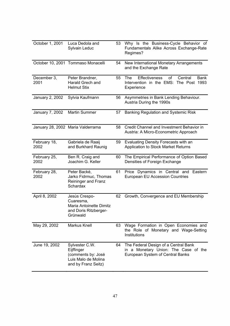
47

October 1, 2001 Luca Dedola and Sylvain Leduc

53 Why Is the Business-Cycle Behavior of Fundamentals Alike Across Exchange-Rate Regimes?

October 10, 2001 Tommaso Monacelli 54 New International Monetary Arrangements and the Exchange Rate

December 3, 2001

Peter Brandner, Harald Grech and Helmut Stix

55 The Effectiveness of Central Bank Intervention in the EMS: The Post 1993 Experience

January 2, 2002 Sylvia Kaufmann 56 Asymmetries in Bank Lending Behaviour. Austria During the 1990s

January 7, 2002 Martin Summer 57 Banking Regulation and Systemic Risk

January 28, 2002 Maria Valderrama 58 Credit Channel and Investment Behavior in Austria: A Micro-Econometric Approach

February 18, 2002

Gabriela de Raaij and Burkhard Raunig

59 Evaluating Density Forecasts with an Application to Stock Market Returns

February 25, 2002

Ben R. Craig and Joachim G. Keller

60 The Empirical Performance of Option Based Densities of Foreign Exchange

February 28, 2002

Peter Backé, Jarko Fidrmuc, Thomas Reininger and Franz Schardax

61 Price Dynamics in Central and Eastern European EU Accession Countries

April 8, 2002 Jesús Crespo-Cuaresma, Maria Antoinette Dimitz and Doris Ritzberger-Grünwald

62 Growth, Convergence and EU Membership

May 29, 2002 Markus Knell 63 Wage Formation in Open Economies and the Role of Monetary and Wage-Setting Institutions

June 19, 2002 Sylvester C.W. Eijffinger (comments by: José Luis Malo de Molina and by Franz Seitz)

64 The Federal Design of a Central Bank in a Monetary Union: The Case of the European System of Central Banks

48

July 1, 2002 Sebastian Edwards and I. Igal Magendzo (comments by Luis Adalberto Aquino Cardona and by Hans Genberg)

65 Dollarization and Economic Performance: What Do We Really Know?

July 10, 2002 David Begg (comment by Peter Bofinger)

66 Growth, Integration, and Macroeconomic Policy Design: Some Lessons for Latin America

July 15, 2002 Andrew Berg, Eduardo Borensztein, and Paolo Mauro (comment by Sven Arndt)

67 An Evaluation of Monetary Regime Options for Latin America

July 22, 2002 Eduard Hochreiter, Klaus Schmidt-Hebbel and Georg Winckler (comments by Lars Jonung and George Tavlas)

68 Monetary Union: European Lessons, Latin American Prospects

July 29, 2002 Michael J. Artis (comment by David Archer)

69 Reflections on the Optimal Currency Area (OCA) criteria in the light of EMU

August 5, 2002 Jürgen von Hagen, Susanne Mundschenk (comments by Thorsten Polleit, Gernot Doppelhofer and Roland Vaubel)

70 Fiscal and Monetary Policy Coordination in EMU

August 12, 2002 Dimitri Boreiko (comment by Ryszard Kokoszczyński)

71 EMU and Accession Countries: Fuzzy Cluster Analysis of Membership

August 19, 2002 Ansgar Belke and Daniel Gros (comments by Luís de Campos e Cunha, Nuno Alves and Eduardo Levy-Yeyati)

72 Monetary Integration in the Southern Cone: Mercosur Is Not Like the EU?

August 26, 2002 Friedrich Fritzer, Gabriel Moser and Johann Scharler

73 Forecasting Austrian HICP and its Components using VAR and ARIMA Models

49

September 30, 2002

Sebastian Edwards 74 The Great Exchange Rate Debate after Argentina

October 3, 2002

George Kopits (comments by Zsolt Darvas and Gerhard Illing)

75 Central European EU Accession and Latin American Integration: Mutual Lessons in Macroeconomic Policy Design

October 10, 2002

Eduard Hochreiter, Anton Korinek and Pierre L. Siklos (comments by Jeannine Baillu and Thorvaldur Gylfason)

76 The Potential Consequences of Alternative Exchange Rate Regimes: A Study of Three Candidate Regions

October 14, 2002 Peter Brandner, Harald Grech

77 Why Did Central Banks Intervene in the EMS? The Post 1993 Experience

October 21, 2002 Alfred Stiglbauer, Florian Stahl, Rudolf Winter-Ebmer, Josef Zweimüller

78 Job Creation and Job Destruction in a Regulated Labor Market: The Case of Austria

October 21, 2002 Elsinger, Alfred Lehar and Martin Summer

79 Risk Assessment for Banking Systems