Embed Size (px)
Citation preview

Basel Committee on Banking Supervision
Working Paper 38
Assessing the impact of Basel III: Evidence from macroeconomic models: literature review and simulations April 2021

The Working Papers of the Basel Committee on Banking Supervision contain analysis carried out by experts of the Basel Committee or its working groups. They may also reflect work carried out by one or more member institutions or by its Secretariat. The subjects of the Working Papers are of topical interest to supervisors and are technical in character. The views expressed in the Working Papers are those of their authors and do not represent the official views of the Basel Committee, its member institutions or the BIS.
This publication is available on the BIS website (www.bis.org/bcbs/).
Grey underlined text in this publication shows where hyperlinks are available in the electronic version.
© Bank for International Settlements 2021. All rights reserved. Brief excerpts may be reproduced or translated provided the source is stated.

Assessing the impact of Basel III: Evidence from macroeconomic models: literature review and simulations iii
Contents
List of members of the Research Group work stream ...................................................................................................... vii
Executive summary ........................................................................................................................................................................... 1
Introduction ......................................................................................................................................................................................... 3
1. Literature review .............................................................................................................................................................. 3
1.1 Operational macroeconomic models ..................................................................................................................... 4
1.1.1 Standard quantitative DSGE models ..................................................................................................... 4
1.1.2 Empirical macro models........................................................................................................................... 13
1.1.3 Quantitative results of available simulations ................................................................................... 16
1.2 Alternative modelling approaches (mostly stylised/qualitative models) ................................................ 17
1.2.1 Modelling financial crises and the benefits of banking regulation ........................................ 18
1.2.2 Models including a shadow banking sector .................................................................................... 27
1.2.3 Modelling the effects of other kinds of public policies ............................................................... 28
1.3 Main conclusions of Part 1 ........................................................................................................................................ 33
2. Model simulations ........................................................................................................................................................ 33
2.1 Definition and implementation of scenarios...................................................................................................... 34
2.1.1 Model calibration ....................................................................................................................................... 34
2.1.2 Scenario definition ..................................................................................................................................... 35
2.2 Main conclusions drawn from the simulations ................................................................................................. 36
2.2.1 On the level of macroeconomic variables ........................................................................................ 37
2.2.2 On business cycle fluctuations .............................................................................................................. 41
2.2.3 On the transition from Basel II to Basel III ........................................................................................ 41
2.2.4 On the transmission of shocks .............................................................................................................. 42
2.3 Conclusions of simulation exercises and suggestions for next steps ...................................................... 44
3. General conclusion ....................................................................................................................................................... 45
References .......................................................................................................................................................................................... 46
Annex 1: Measurement issues associated with the scenarios ....................................................................................... 51
1. Discussion about the measurement of bank default probability .............................................................. 51
2. Discussion about the calibration of bank risk and the conduct of the exercise .................................. 51
Annex 2: Definition of the scenarios ........................................................................................................................................ 53

iv Assessing the impact of Basel III: Evidence from macroeconomic models: literature review and simulations
Annex 3: Detailed analysis of the country results ............................................................................................................... 55
1. Euro area by the European Central Bank ............................................................................................................. 55
1.1 Model description ......................................................................................................................................................... 55
1.2 Key mechanisms governing the relationship between capital requirements and economic activity and welfare ....................................................................................................................................................... 55
1.2.1 Impact of capital requirements on economic activity .................................................................. 55
1.2.2 Impact of capital requirements on welfare....................................................................................... 56
1.3 The impact of capital requirements on the level of macroeconomic variables ................................... 56
1.4 Impact on the volatility of macroeconomic variables .................................................................................... 58
1.5 Transitions from Basel II to Basel III ....................................................................................................................... 58
1.5.1 Capital requirements ................................................................................................................................. 58
1.5.2 LCR implementation .................................................................................................................................. 60
1.6 Response to shocks: Covid-19 scenario ............................................................................................................... 61
2. Euro area analysis on the basis of de Bandt and Chahad (2016) ............................................................... 61
2.1 Model specificities ........................................................................................................................................................ 61
2.2 Steady-state comparison ........................................................................................................................................... 61
2.2.1 Solvency .......................................................................................................................................................... 62
2.2.2 LCR .................................................................................................................................................................... 62
2.3 Transition to the new steady state ......................................................................................................................... 62
2.3.1 Solvency scenario ....................................................................................................................................... 62
2.3.2 LCR scenario: transition from 60% to 100% ..................................................................................... 64
3. United States by the Board of Governors of the Federal Reserve System ............................................. 64
3.1 Key mechanisms ............................................................................................................................................................ 64
3.2 Results on the level of macroeconomic variables ............................................................................................ 65
3.3 Results on the volatility of macroeconomic variables .................................................................................... 65
3.4 Transitions from Basel II to Basel III ....................................................................................................................... 66
3.5 Steady-state comparison with LCR requirement .............................................................................................. 67
4. Euro area by Bank of France with Gerali et al (2010) ...................................................................................... 68
4.1 Model specificities, steady state comparison and transition to steady state ........................................ 68
4.2 Impact of Covid-19 scenario..................................................................................................................................... 70
5. Norway by Central Bank of Norway....................................................................................................................... 72
5.1 Model description ......................................................................................................................................................... 72
5.2 The effects of capital requirements on real economic activity and welfare .......................................... 73
5.3 Steady-state analysis of changes in capital requirements ............................................................................ 74

Assessing the impact of Basel III: Evidence from macroeconomic models: literature review and simulations v
5.4 Steady-state analysis of changes in LCR requirements ................................................................................. 79
5.5 Transitions from Basel II to Basel III ....................................................................................................................... 80
5.5.1 Transition to solvency requirements................................................................................................... 80
5.5.2 Transition to LCR requirements ............................................................................................................ 83
5.6 Business cycle moments: Basel II vs Basel III comparison............................................................................. 84
Annex 4: Parameterisation of 3D model by the European Central Bank .................................................................. 85
Annex 5: Parameterisation of 3D model by the Board of Governors of the Federal Reserve System ........... 86
Annex 6: Parameterisation of NEMO (Central Bank of Norway) and endogenous financial crisis ................. 87
1. Parameterisation, calibration and estimation .................................................................................................... 87
2. Endogenous financial crises in NEMO .................................................................................................................. 89


Assessing the impact of Basel III: Evidence from macroeconomic models: literature review and simulations vii
List of members of the Research Group work stream1
Co-Chairs Mr Olivier de Bandt, Bank of France Mr Michael Straughan, Bank of England
Belgium Mr Jolan Mohimont National Bank of Belgium Canada Mr Josef Schroth Bank of Canada France Mr Jean-Guillaume Sahuc
Mr Valerio Scalone Bank of France
Germany Ms Sigrid Roehrs Deutsche Bundesbank Italy Ms Roberta Fiori Bank of Italy Japan Mr Hibiki Ichiue Bank of Japan Norway Mr Yasin Mimir Central Bank of Norway United States Mr Bora Durdu Board of Governors of the Federal Reserve System European Central Bank
Mr Markus Behn Ms Katarzyna Budnik Mr Kalin Nikolov
ECB
Mr Greg Sutton Financial Stability Institute
Secretariat Mr Martin Birn Bank for International Settlements
1 Comments by other members of the Research Group are gratefully acknowledged.


Assessing the impact of Basel III: Evidence from macroeconomic models: literature review and simulations 1
Executive summary
To quantitatively assess the impact of Basel III reforms from a macroeconomic perspective, structural quantitative macroeconomic models have been developed that capture the transmission mechanisms of prudential policies. Central banks and supervisory agencies have been at the forefront in the development and application of such models. This report gives an overview of the literature. The first part of this report reviews the different channels of transmission of financial shocks (including regulatory changes) highlighted in the literature in the last 15 years. It distinguishes between, on the one hand, standard quantitative Dynamic Stochastic General Equilibrium models and empirical time-series macroeconomic models routinely used by central banks and, on the other hand, alternative models that investigate potential additional channels, and new issues.
The conclusion of this journey into the world of macroeconomic models is that a very large number of new models have been made available since BCBS (2010), but standard models still concentrate mostly on capital requirements and more rarely on liquidity. Alternative models consider other policies (unconventional monetary policies, etc) as well as new, highly relevant challenges like interactions with the shadow banking system. However, the latter models are not yet sufficiently operational to allow an empirical assessment of the impact of the regulatory changes.
The second part of this report provides a simulation of regulatory scenarios replicating the implementation of Basel III reforms, using “off-the-shelf” macro-finance models at the European Central Bank, the Board of Governors of the Federal Reserve System, the Central Bank of Norway and the Bank of France. These simulations provide novel estimates of the impacts of Basel III. The variety of models and jurisdictions on which the macroeconomic impact of Basel III is assessed ensures the robustness of the findings. Some models do not measure the benefits, so that the latter may be inferred by difference with the output of the models that assess both costs and benefits.
Long-term impact of a move from Basel II to Basel III (solvency) Table 1
Unit GDP % dev
Bank probability of default % pts dev
Cost of crisis (% of GDP), % pts dev
Euro area with 3D model 1.2% -7.50 -2.55%(1)
Euro area with de Bandt and Chahad (2016) 0.2% -0.15 -0.01%
Euro area with Gerali et al (2010) framework (cost approach)
-0.4% NaN NaN
United States 0.9% -9.21 -3.36%(1)
Norway (moderate crisis prob. and severity) -0.2% -0.16(2) -0.85%(3)
Norway (high crisis prob. and severity) 2.1% -1.63(2) -4.39%(3)
The move from Basel II to Basel III is measured by a 5 percentage point increase in capital requirements. (1) Change in bail out costs. (2) Change in the probability of a financial crisis. (3) Change in the cost of a financial crisis.
In a nutshell, whenever the costs and benefits of regulation are introduced in the model, the effects of Basel III are positive on GDP (this is the case for the 3D model applied to the euro area and the United States, as well as the model by de Bandt and Chahad (2016) with run probability). This holds both for the United States and euro area economies. The positive effect of Basel III on GDP may however be associated in the transition to Basel III by a temporary slowdown accommodated by monetary policy. In additional exercises, we assess the costs related to the transition from Basel II to Basel III. First, the Central Bank of Norway’s NEMO model concludes that the net benefits of Basel III depend on the magnitude of the crisis probability and severity. In the case of moderate crisis probability and severity, Basel III has a small negative effect on GDP although it reduces both the crisis probability and the severity. However, when both the probability and the severity nearly double, Basel III has positive effects on GDP as its net

2 Assessing the impact of Basel III: Evidence from macroeconomic models: literature review and simulations
benefits become substantial. Second, using the Gerali et al (2010) framework for the euro area, which only identifies the cost of implementation of the regulation, yields a negative effect on GDP, but this results is an obvious consequence of the absence of modelling of the benefits of regulation. Comparing these results with those of the other models for the euro area, the long-run benefits of the Basel III framework could be estimated between 0.6 and 1.6% of GDP.
All in all, one needs to emphasise that the results of the models crucially depend on the assumptions regarding the magnitude and the sensitivity of the bank default probability or the financial crisis probability. This is consistent with BCBS (2010) and Birn et al (2020). Expectations regarding the likely impact of the regulation also play a significant role in the positive assessment of the impact of Basel III regulations.
Furthermore, all models exhibit a decrease in volatility when moving from Basel II to Basel III, but the impact is not very sizeable.
In addition, the models are used to provide a first assessment of the resilience of the post-Basel III banking system to very large shocks replicating the current Covid-19 environment.
While significant advances have been made for the modelling of solvency requirements, the assessment of liquidity requirements is still an area for research, as most models still concentrate on the costs of liquidity. Preliminary evidence presented in the report based on general equilibrium models indicates that the macroeconomic impact of Basel III has the expected positive sign on GDP; however, the effect is not large. More work is still needed to provide the full assessment of the costs and benefits, in particular in terms of lower contagion risk.

Assessing the impact of Basel III: Evidence from macroeconomic models: literature review and simulations 3
Introduction
When assessing the impact of the Basel III regulations, it is important to consider the broader macroeconomic impact of the regulations in addition to the microeconomic impact on institutions. Such considerations were present in the initial development of Basel III, as discussed in the Basel Committee’s Long-term Economic Impact (LEI) report (BCBS (2010)) and the MAG (2010) report. After a decade, it is useful to revisit these issues in order to take stock of the large number of macroeconomic models developed since then, which include a much more detailed description of the interaction between the financial sector and the rest of the economy, as well as other potential trade-offs.2 In this report, we provide a map of the literature on macroeconomic models, defined here as the quantification of interactions between financial behaviours and macroeconomic activity. By focusing on this particular tool, we are complementing BCBS (2019) which examined the literature updating the entire cost-benefit-analysis approach set out in the LEI and MAG.
The aim of the report is to support efforts to build models that can be used to estimate and evaluate the impact of post-2010 reforms. As noted, we focus on the impact of the reforms in terms of macroeconomic variables; ie we are interested in the evolution of GDP and its key components, such as consumption and investment, over time.
The report has two parts:
• First, we survey the literature, characterise relevant economic channels and document what the literature is already implying about the impact of reforms. We distinguish between, on the one hand, standard quantitative Dynamic Stochastic General Equilibrium (DSGE) models and empirical time-series macroeconomic models routinely used by central banks, and on the other hand, alternative models that investigate additional channels, as well as new issues. We conclude with recommendations on the kind of model that needs to be built. Our recommendation trades off including all the relevant channels against technical feasibility and usability.
• Second, we present the results of simulation exercises where we compare some of the models surveyed in the first part and in current use by regulators. The simulations provide examples of the sort of outputs that the models currently being used by regulators can provide. We also consider the impact of a large-scale shock, Covid-19-like, in order to assess the resilience of the banking system.
1. Literature review
The objective of this literature review is to set out the current ”technological state of play” in the academic literature of macroeconomic models that will allow us to evaluate the impact of Basel III (and other financial market regulation).
There are a large number of approaches taken by macroeconomic models documented in the academic literature. The approach followed in this report is to limit the analysis to those models that allow an assessment of the impact of the reforms on both the financial sector and the real economy. For this
2 In contrast, the LEI and MAG rely mostly on real sector macroeconomic models without a banking sector and the transmission
of regulation was implemented through a calibration of the transmission of higher regulatory requirements on bank lending rates (ie prices) assuming a full pass through of a higher cost of capital. Since then, the academic literature investigated the direct impact of higher requirements on loan supply (in particular loan quantities). See BCBS (2019).

4 Assessing the impact of Basel III: Evidence from macroeconomic models: literature review and simulations
reason, we place some emphasis on general equilibrium (GE) models that permit consideration of possible trade-offs beyond the financial sector. Three types of models are considered:
1. Standard quantitative DSGE models, which have experienced much improvement since the Great Financial Crisis (GFC) with the introduction of fully-fledged banking sectors relative to the earlier generation of models.
2. Empirical macro models, which include a banking sector (as above) and provide quantitative results.
3. Alternative modelling approaches consisting of more stylised/qualitative DSGE models that investigate new channels of transmission of regulatory changes as well as new issues (Section 1.2).
For each of these model types, three key dimensions are investigated:
1. The policies explicitly included. For example, do the models focus on capital increases, liquidity policy or both? Is there any allowance for other policies developed by the Basel Committee, such as the quality of capital?
2. The transmission channels in the model. In particular, what “shocks” can be applied to the model? How do these shocks affect the financial sector and how are they propagated through the macroeconomy?
3. The outputs from the models. Clearly, changes in GDP (including volatility) will be useful. But what about social welfare? Do outputs include benefits (eg increase in GDP or reduction in crisis costs) resulting from, eg, reducing endogenous (negative) shocks?
The rest of the literature review distinguishes between operational economic models that are used by policy institutions, including standard quantitative models and empirical macro models (Section 1.1), as well as new modelling avenues and other models available in the economic literature (Section 1.2).
1.1 Operational macroeconomic models
Policy institutions rely on various types of macro models that are used to assess the impact of reforms. Two types of operational macroeconomic models are presented here:
• Standard DSGE models that put emphasis on micro-founded economic behaviour, as well as the identification of channels of transmission of financial regulation (Section 1.1.1).
• Time series econometric models that concentrate on the empirical fit to macroeconomic data available and provide quantitative estimates of impact of reforms on macroeconomic variables (Section 1.1.2).
1.1.1 Standard quantitative DSGE models
DSGE models were developed in central banks in the 1990s and 2000s, but initially they were mainly monetary models used to define optimal monetary policy. The Smets and Wouters (2003) model is a good illustration of this kind of New-Keynesian General Equilibrium model where macroeconomic cycles are explained by real and nominal frictions. On the financial side, Bernanke et al (1996) introduced asymmetric information in the financing of firms, so that lending rates include a yield spread that fluctuates over the cycle and creates acceleration effects, so that financial cycles may amplify real cycles. Similarly, lending cycles introduced by Kiyotaki and Moore (1997), where non-financial firms are credit-constrained and lending is limited by the amount of collateral they can pledge, is a backbone of many subsequent macroeconomic models. According to this collateral channel, also extended to mortgage loans to

Assessing the impact of Basel III: Evidence from macroeconomic models: literature review and simulations 5
households, the price of collateral plays a major role in tightening financial constraints in general equilibrium, amplifying the effects of exogenous shocks.
Since the GFC, these models have been expanded to include a more complete banking sector that takes into account banks’ balance sheet constraints and additional transmission channels of financial shocks, taking on board the results of models developed in the banking and finance literature. The majority of papers on financial cycles focuses on frictions affecting financial intermediaries. For example, Bernanke (2018) argues that the unfolding of the GFC in the United States can be characterised by an amplification through the financial sector of a shock originating in the household sector.3
In this section, we describe the building blocks of these quantitative DSGE models, with a particular focus on models that incorporate directly banking regulation or develop channels of transmission that would allow a future integration of banking regulation. We discuss the following characteristics of these models in succession:
1. The channels of transmission (Section 1.1.1.1).
2. The types of regulations that are investigated and the results found by these models regarding the impact of Basel III (Section 1.1.1.2).
1.1.1.1 Channels of transmission
Table 2 below sets out the papers that are summarised in this section.
Standard quantitative DSGE models by channels of transmission Table 2
Channels Papers
Net worth/occasionally binding capital constraints
Gertler and Karadi (2011), Meh and Moran (2010), Gerali et al (2010), Clerc et al (2015), Mendicino, Nikolov, Suarez and Supera (2018, 2020), Jondeau and Sahuc (2018), Kravik and Mimir (2019), Kockerols, Kravik and Mimir (2021) (Central Bank of Norway’s NEMO model)
Bank runs Angeloni and Faia (2013), Gertler and Kiyotaki (2015)
Banks’ funding and liquidity Covas and Driscoll (2014), De Nicolò and Luchetta (2014), de Bandt and Chahad (2016), Begenau (2020), Van den Heuvel (2019), Hoerova et al (2018), Boissay and Collard (2016)
Risk taking Martinez-Miera and Suarez (2014)
The models used in policy institutions are usually built around a core element that features occasionally binding intermediary capital constraints (Section 1.1.1.1.1). There is a well-developed theory on this channel in the context of DSGE modelling, highlighting its relevance and feasibility. This channel is complemented in some cases by the channels of bank runs (also treated in Section 1.1.1.1.1), funding liquidity and collateral (Section 1.1.1.1.2) and banks’ risk taking channel (Section 1.1.1.1.3).
1.1.1.1.2 Occasionally binding intermediary capital constraints
The net worth of financial intermediaries, “banks”, may affect their access to outside funding through concerns about bank moral hazard. Banks cannot roll over outside funding (“bank run”) when net worth is low and then they are forced to reduce lending (a “credit crunch”).4 The level of bank net worth determines
3 Bernanke (2018) writes “Although the deterioration of household balance sheets and the associated deleveraging likely
contributed to the initial economic downturn and the slowness of the recovery, I find that the unusual severity of the Great Recession was due primarily to the panic in funding and securitisation markets, which disrupted the supply of credit.”
4 To fix ideas we will refer to financial intermediaries as banks and use the term lending, or loans, as a stand-in for assets that are typically not held directly by savers but by banks as intermediaries.

6 Assessing the impact of Basel III: Evidence from macroeconomic models: literature review and simulations
the probability that the bank becomes funding constrained as a result of (possibly small) exogenous shocks. Low bank net worth therefore induces banks to reduce lending as a precaution and increases lending spreads. An adverse exogenous shock that occurs against the backdrop of low bank net worth creates non-linear dynamics and triggers a credit crunch.
This channel is often combined with other channels in the literature, which leads to even greater effects: low net worth implies that the probability of failure increases so that the bank’s funding costs increase as investors request a higher interest rate. They are reviewed more generally in Section 1.1.1.1.2.
We present earlier models (Meh and Moran (2010), Gerali et al (2010), Gertler and Karadi (2011) and Angeloni and Faia (2013)) before looking at more sophisticated and operational models (Mendicino et al (2018, 2020), Jondeau and Sahuc (2018), the Central Bank of Norway’s NEMO model as in Kravik and Mimir (2019) and Kockerols et al (2021)).
a) Meh and Moran (2010)
The Meh and Moran model, one of the first DSGE models with a banking sector, highlights the role of capital although regulation is not directly included per se. In previous models, banks’ liability side consisted only of deposits leaving no direct role for bank capital. The novelty of the model is that bank capital emerges endogenously to solve an asymmetric information problem between bankers and their creditors: banks can attract loanable funds if they have capital, because capital provides an incentive to monitor the projects when there is moral hazard by firms (Holmström and Tirole (1997)).
Bank capital creates a new channel for the propagation and amplification of shocks. A negative technology shock reduces bank lending profitability, making it harder for banks to attract loanable funds. Bank capital, which is mostly composed of retained earnings, is negatively affected by the technology shock so that bank lending falls, along with aggregate investment. Lower investment depresses bank earnings even more, which translates into lower bank capital in future periods and thus further decreases in aggregate investment.
Following a negative technology shock, the weight of deposits in financing a given-size project must fall, so that banks must hold more capital per unit of loan, hence the required capital ratio increases. Business fluctuations are therefore amplified when the bank capital channel is active.
b) Gerali et al (2010)
Gerali et al (2010) is the first DSGE model that directly includes prudential regulation, in this case a capital requirement while liquidity is introduced in a rather crude way. Banks provide loans to both households and non-financial firms, and banks fund themselves using household deposits and equity capital. It is assumed that banks cannot raise additional equity. They set interest rates in a monopolistically competitive fashion subject to adjustment costs, which leads to imperfect and sluggish interest rate pass-through from the policy rate to loan and deposit rates. Banks choose the overall level of lending and funding, with capital requirements adjusted with asset specific risk weights.5 The profit function of a typical bank includes a quadratic cost when there is a deviation from the target ratio, so that banks incur a cost if they fail to meet their capital-to-asset ratio target. Such a model is used by different policy institutions, notably Bank of Italy, Central Bank of Norway’s NEMO model and Bank of France. The Central Bank of Norway’s NEMO Model (Kravik and Mimir (2019)) includes a core DSGE model inspired by the Gerali et al (2010) model, additionally modified to include foreign borrowing by banks in an open economy framework (see Section 1.1.2). Some of the simulations presented in Part 2 are based on a Markov regime-switching version of this model with financial crisis dynamics (Kockerols et al (2021)).
5 Asset-specific risk weights are not part of the original Gerali et al (2010) model, but some models building on that paper, like
the Nemo model (see below), incorporate them in order to conduct some analyses based on time-varying risk weights.

Assessing the impact of Basel III: Evidence from macroeconomic models: literature review and simulations 7
c) Gertler and Karadi (2011)
Gertler and Karadi (2011) introduce private intermediaries (banks) in a standard DSGE model to study the impact of unconventional monetary policy modelled as central bank credit intermediation.
Private intermediaries hold financial claims (equivalent to equities) on non-financial corporations (NFCs) financed with their net worth and households’ deposits. They face an agency problem with their depositors, which introduces a constraint on their leverage ratio. In contrast, the central bank does not face an agency problem but is less efficient in providing credit to the private sector (it pays a deadweight cost per unit of credit).
In this context, when a financial shock hits the economy (modelled as a reduction in capital quality, but it could also be a tightening of solvency regulation), the value of intermediaries’ financial claims on private non-financial corporations (PNFC) declines. The leverage constraint implies that intermediaries sell their assets and reduce credit, which amplifies the impact of the shock. The Bank of Canada uses a variation of this model.
d) Angeloni and Faia (2013)
The DSGE model by Angeloni and Faia (2013) features nominal rigidities and a banking sector where banks are subject to runs by depositors. The probability of bank runs increases with the level of leverage. In this approach, expansionary shocks increase banks’ leverage, and therefore also bank risk, and the probability of runs. Angeloni and Faia show that constraints on leverage through regulation reduce the probability of runs.
e) Mendicino, Nikolov, Suarez and Supera (2018, 2020)
The model set out in these papers is an operational DSGE model that can be used for simulations of prudential policies. Some of the simulations presented in Part 2 are based on this model. The model builds on that of Clerc et al (2015) (the “3D” model) which introduces financial intermediation and three layers of default into an otherwise standard DSGE model. The authors extend the model by introducing nominal rigidities and monetary policy. This extension considers households who borrow to buy houses and firms who borrow in order to invest in productive projects. Banks are essential to intermediate funds between savers and borrowers in this economy so financial instability and bank failures have a large negative impact on lending and economic activity. The model features a representative worker-saver household, a representative worker-borrower household, entrepreneurs (who provide equity funding to firms), bankers (who provide equity funding to banks), one period firms and banks.
There is an incentive for risk taking by banks given the existence of deposit insurance and that the actions of banks are unobserved (moral hazard). There is a bank capital channel for transmitting the impact of shocks. Loan losses reduce bank capital and subsequently reduce lending to the real economy due to the binding capital requirement. In addition, there is a bank funding cost channel: higher default probability for banks increases the interest rate on uninsured bank debt and raises the cost of providing loans to the real economy. Conversely, when the capital ratio is too low, the probability of bank default is high, so that increasing capital may lower the weighted average cost of bank funding, implying higher steady state bank lending and GDP (this is demonstrated in Part 2 of this review).
The model also includes deadweight default losses: the failure of banks and firms leads to damage to the economy’s productive capacity. They allow calculation of an optimal level of capital, trading-off the short-run negative impact of capital constraints on lending and the deadweight loss of bank failures.
In the model, there are transmission channels for both capital and liquidity regulation. First, capital requirements affect the economy in two main ways. On the one hand, since equity is more expensive than debt, higher capital requirements may contribute positively to banks' weighted-average cost of funding. On the other hand, since some funding is uninsured, higher capital requirements reduce

8 Assessing the impact of Basel III: Evidence from macroeconomic models: literature review and simulations
interest rates on uninsured bank debt. This reduces banks’ weighted-average cost of funds. When the risk of bank default is high, the cost of uninsured bank debt dominates and higher capital requirements actually reduce banks’ overall funding costs allowing them to lend more cheaply. This is why output sometimes increases in the long run with higher capital requirements. Conversely, when the risk of bank default is low, the compositional effect (driven by the fact that equity is more expensive than debt) dominates and higher capital requirements increase banks’ cost of funding, making it more expensive to lend to firms and households.
Second, liquidity requirements (liquidity coverage ratio (LCR) and net stable funding ratio (NSFR)) may be introduced in the model as additional costs to banks from having to: (i) substitute low yielding high-quality liquid assets (HQLA) for higher yielding loans in order to meet the LCR requirement; or (ii) fund with more expensive long-term debt, to meet the NSFR requirement. These costs increase lending rates with a contractionary effect on lending and real activity. However, the model is not rich enough to analyse the benefits of the LCR and the NSFR.
f) Jondeau and Sahuc (2018)
Two types of banks are introduced in the model by Jondeau and Sahuc (2018): deposit banks, which receive deposits from households and provide (risky) loans to merchant banks; and merchant banks (or equivalently shadow banks), which use short-term loans from deposit banks to buy long-term claims on producing firms’ assets. This description of the banking sector allows merchant banks to borrow from deposit banks by posting collateral assets, and thus to generate an amplification phenomenon if the value of these assets falls.
Indeed, firms finance their investment in capital equipment by selling a long-term claim on their assets to merchant banks. Merchant banks obtain funds from deposit banks and use the firm’s securities as collateral to secure the loan. Their revenues from the firm’s securities depend not only on the shock to the firm’s capital investment but also on the cross-sectional dispersion in the quality of the capital equipment. If the quality is low, the value of merchant banks’ assets is low and the collateral may be insufficient to secure the loan. In that case, merchant banks have to delever by selling assets, in order to reduce their debt to match the available collateral. In case of crisis, this mechanism can result in an increase in deposit banks’ leverage and a decrease in merchant banks’ leverage with the fall in the market value of the assets merchant banks hold, as observed in 2008. For some banks, the loss on the firm’s securities can be so large that the bank defaults. In such an instance, the remaining assets are liquidated by the deposit banks at a cost. Some deposit banks may have insufficient assets to repay their deposits and therefore default. Because deposits are guaranteed by an insurance mechanism, the cost of the deposit bank’s default is eventually borne by the government.
In this model, capital shortfall (also named stress expected loss, SEL) is the additional equity that would be necessary for deposit banks to repay their deposits in bad times. Regulations can be introduced in the framework to address the effects of several reforms.
1.1.1.1.2 Funding, liquidity and collateral constraints
Like other borrowers (as indicated above with liquidity constraints on NFC and households, following Kiyotaki and Moore (1997)), banks face funding and liquidity constraints, compounded by the risk of bank runs. Regulation aims at limiting that risk by imposing constraints on the maturity of funding sources, or on the liquidity of assets to avoid bank runs. Models in this part of the literature include De Nicolò et al

Assessing the impact of Basel III: Evidence from macroeconomic models: literature review and simulations 9
(2014) in partial equilibrium, or in general equilibrium as in Covas and Driscoll (2014)6 or de Bandt and Chahad (2016), which were previously reviewed in BCBS (2016). Readers can refer to that study for more detail. Below, we focus on some more recent papers that also utilise these transmission channels.
a) Van den Heuvel (2019)
The Van den Heuvel model provides a methodology for estimating the welfare costs (although not the benefits) of liquidity and capital regulation.7 The model embeds the role of liquidity-creating banks in an otherwise standard general equilibrium growth model. Besides banks, the model also features firms and households who own the banks and the firms. Because of the preference for liquidity on the part of households and firms, liquid assets, such as bank deposits and government bonds, command a lower rate of return than illiquid assets, such as bank loans and equity. The spread between the two is the convenience yield of the liquid instrument. The model incorporates a rationale for the existence of both capital and liquidity regulation, based on a moral hazard problem created by deposit insurance. But these regulations also have costs, as they reduce the ability of banks to create net liquidity.
Capital requirements directly limit the fraction of assets that can be financed with liquid deposits, while liquidity requirements reduce net liquidity transformation by banks. Requiring banks to hold more HQLA crowds out other users of these assets, such as investment funds, insurers, pension funds, etc, increasing scarcity of safe assets. At the same time, it has the effect of making financial intermediation by banks more costly, potentially reducing credit. The total macroeconomic costs consist of costs from reduced access to liquidity, reduced credit and, consequently, potential reductions in investment and output.
The model implies that the macroeconomic costs depend primarily on the spread between the risk-adjusted required return on equity and the average interest rate on bank deposits. Formally, the macroeconomic costs are measured as the welfare cost, a summary measure of all present and future costs due to lost production and reduced liquidity, expressed as a percentage of GDP.
b) Boissay and Collard (2016)
In the Boissay and Collard (2016) model, the banking sector allocates households’ savings. Households can also lend directly through bond markets. Banks are heterogeneous,8 creating an interbank market where some banks are lenders and others borrowers. Borrowing banks can divert some funds that lending banks cannot take back. This creates an agency problem. Banks divert more when they have high leverage and when their liquidity is lower (they hold a lower value of government bonds).
Since banks do not fully internalise the effects of their funding decisions, capital and liquidity regulations address these externalities. On the one hand capital and liquidity regulations may reinforce each other since capital requirements affect banks’ portfolio decisions whereas liquidity requirements influence banks to buy more bonds and lend less. On the other hand, in equilibrium some counteracting effects can arise since more stringent liquidity requirements can encourage greater purchases of government bonds, therefore reducing government bond yields and pushing households to put more savings in deposits, increasing banks’ leverage. However, this counteracting effect is quantitatively smaller than the reinforcing effect for a realistic calibration of the model.
6 Covas and Driscoll (2014) highlight the importance of price adjustments for loans and securities as well as the Net Interest
Income (NII) channel. When loan and security prices are not allowed to adjust (eg in partial equilibrium), the imposition of liquidity and capital requirements have relatively substantial impacts, leading to a sizeable contraction in credit. However, in a general equilibrium framework, lower loan supply and greater demand for securities imply loan rates increase and returns on securities drop, thereby dampening the results.
7 Hoerova (2018) et al provides a description of the model by Van den Heuvel based on earlier versions of the paper. 8 See Section 1.2.2 for a discussion of another type of bank heterogeneity: shadow banks and regulated banks.

10 Assessing the impact of Basel III: Evidence from macroeconomic models: literature review and simulations
c) Begenau (2020)
In the model of Begenau (2020), banks hold risky assets (productive capital used to supply goods) and non-risky assets (government bonds) funded with bank equity and deposits. Regulation enters the model through a bank’s equity requirement as a fraction of risk-weighted assets. There is an always-binding regulatory constraint on the ratio of a bank’s equity to risky assets.
The model has a few uncommon features. One is that deposits enter households’ utility function. Deposits are cheaper compared to equities, because they offer a convenience yield. In addition, there is a bank dependent production sector responsible for a fraction of total GDP. Output in this sector is a function of banks’ productive capital (which correspond to the risky asset) and of a stochastic banks’ productivity level. Specifically, banks’ productivity depends on their monitoring effort. Higher monitoring increases the average productivity level and lowers its variance.
There are several channels by which higher capital requirements are transmitted to the real economy and thus impact welfare:
1. Higher equity requirements force the bank to accumulate capital, which increases banks’ financing costs.
2. Higher equity requirements also reduce bank deposits. This is welfare-decreasing for households that derive utility from deposits. However, it also decreases the deposit rate (since the marginal convenience yield increases), which lowers banks’ financing costs.
3. Finally, higher equity requirements increase banks’ incentive to monitor projects, as shareholders have more “skin in the game”. This lowers banks’ risk and raises their average returns. This decreases the volatility of output and consumption and boosts their average levels.
In sum, total bank funding costs are reduced with higher capital ratios. Higher bank capital requirements (compared to a baseline of 9%) are welfare increasing. Benefits from higher and smoother consumption outweigh the costs of lower deposits.
1.1.1.1.3 Risk taking channel
In order to highlight the risk channel, Martinez-Miera and Suarez (2014) develop a discrete time DSGE model with perfect competition and an infinite horizon. The economy is made of patient agents, who essentially act as providers of funding to the rest of the economy, and impatient agents, who include pure workers, bankers and entrepreneurs. Savers provide a perfectly elastic supply of funds to banks in the form of deposits but cannot directly lend to the final borrowers. Banks finance at least a fraction of their one-period loans with equity capital (ie with funds coming from bankers’ accumulated wealth). Banks complement their funding with fully-insured, one-period deposits taken from patient agents.
Banks finance firms that invest in a good asset or in a bad asset. The bad asset has a lower expected return on average, but a higher return when the economy is in the boom phase of the business cycle: systemic firms are overall less efficient than non-systemic ones. However, it is assumed that, conditional on the systemic shock not occurring, systemic firms yield higher expected returns. As a consequence, systemic risk-taking peaks after long periods of calm. Undercapitalised banks take risk by holding the bad asset.
Regarding the impact of regulation, higher capital ratios:
• discourage investing in the bad asset, ie reduce the proportion of resources going into inefficient systemic investments;
• increase the demand for scarce bank capital in each state of the economy, reinforcing bankers’ dynamic incentives to guarantee that their wealth (invested in bank capital) survives if a systemic shock occurs.

Assessing the impact of Basel III: Evidence from macroeconomic models: literature review and simulations 11
1.1.1.2 Types of regulation investigated
In this section, we revisit the papers to provide a brief summary of the types of regulations (capital or liquidity) that selected papers investigate in more detail. The associated quantitative impact is summarised in Section 1.1.3.
1.1.1.2.1 Impact of solvency regulation
a) Angeloni and Faia (2013)
Angeloni and Faia (2013) show how Basel III (in particular the counter-cyclical component of the capital requirements) helps stabilise the banking system and reduce the fluctuations of the economy. They also show that monetary policy and capital regulation interact, in that (i) monetary policy can improve welfare by responding to asset price or leverage; (ii) countercyclical capital requirements reduce the sensitivity of the economy to monetary policy and productivity shocks.
b) Begenau (2020)
Begenau calibrates her model on US data (1999–2016) and investigates the effect of changing the capital requirement from 9.3% to 12.4%, which amounts to an increase by a third. For households, the higher capital requirement leads to slightly higher consumption (+0.33%) and lower consumption volatility (−18.9%). Output increases marginally by 0.02% and volatility decreases more substantially by 16.8%. To reach this new level of capital requirement, the equilibrium level of deposits falls by 0.86%. The reduction in the deposit rate by 70 basis points leads to an overall reduction in banks’ cost of capital from 1.23% to 0.39%. This reduction makes bank lending much more profitable and encourages banks to increase the credit supply by 2.35%. The reduction in banks’ cost of capital also boosts their profits by 45%.
In general equilibrium, a higher capital requirement leads to lower funding costs, more credit provision and more monitoring and thus less excessive risk-taking by banks. Overinvestment in low-quality bank projects decreases.
c) Mendicino, Nikolov, Suarez and Supera (2020)
Mendicino, Nikolov, Suarez and Supera (2020) highlight differences across agents to show the impact of capital regulations. Borrowers and savers agree up to a point that higher capital requirements are optimal. No one benefits from banks that are too fragile (with a high probability of default). Savers pay taxes to insure deposits at failed banks, which is also the case to some extent for borrowers. Hence, borrowers would equally like banks to be reasonably resilient. Savers prefer banks to be completely safe because they are only taxpayers and are not hurt by higher mortgage rates as they do not borrow.
Borrowers would like a very low sensitivity of capital requirements to borrower default because they are hurt by the pro-cyclicality of lending standards over the business cycle. Savers would like sectoral capital requirements (on NFC and mortgage loans) to adjust to default risk in a way that is similar to that implied by Basel II because they want to keep banks very safe at all times. In addition, in the model, the level of optimal capital requirements is more important for welfare than the cyclical adjustment.
d) Mikkelson and Pedersen (2017)
Mikkelson and Pedersen (2017) use a DSGE model of the Danish economy with a micro-founded banking sector set out in Pedersen (2016) to examine both the short- and long-term costs of economic regulation, defined as the effect on GDP during the first one to three years and the effect after 10 years, respectively.
The DSGE model set out in Pedersen (2016) builds on a number of papers, including Bernanke et al (1999), Kiyotaki and Moore (1997) and Iacoviello (2005). The micro-foundations for the banking sector broadly follow the setup of Gerali et al (2010). One important aspect of the model is that it allows for both the banks’ return on equity and the dividend ratio (the proportion of profits distributed as dividends to
12 Assessing the impact of Basel III: Evidence from macroeconomic models: literature review and simulations
shareholders) to be fixed. In particular, the dividend ratio for banks is set exogenously, reflecting the assumption that shareholders demand a steady stream of dividend payments from banks. The authors point out that the low cost of entry to provide financial services in Denmark means that competition is ”high” and this is a key factor in moderating the effects of higher capital requirements.
The model is used to explore a number of scenarios that progressively ease restrictions in the model to examine the likely costs of capital regulation on the Danish economy. They consider first a scenario with a constant return on equity and fixed dividend ratio and, second, allow return on equity to vary endogenously. Third, they suspend payment of all dividends and, lastly, they impose a higher cost to banks of deviating from their desired capital ratios.
For the first scenario, the authors find that the costs of higher bank capital ratios are within the range of other estimates in the long term, but are more significant in the short term. Easing the constant return-on-equity assumption in the second scenario (ie introducing a “Modigliani-Miller offset” 9 ) significantly reduces the short-term costs and reduces the long-term economic costs to zero. This occurs because the return on equity falls over the longer term, which reduces the need for banks to maintain higher lending spreads. Suspending dividends further reduces the costs. The suspension of dividends has offsetting effects in the model. While it reduces household incomes (households are the ultimate owners of the banks), it also shortens the time it takes for banks to adjust to higher capital requirements. The overall impact is to reduce the impact on economic activity in the short term, while long-term costs remain zero. Lastly, increasing the cost to banks when they deviate from their desired capital ratios increases the size of the short-term adjustment, resulting in costs similar to the second and third scenarios.
1.1.1.2.2 Impact of liquidity regulation
a) Hoerova et al (2018)
Hoerova et al (2018) focusses on the costs and benefits of liquidity regulation. Much of the paper is focussed on demonstrating the positive role that liquidity policy can have on reducing the need for lender of last resort interventions during financial crises. The authors then examine the opportunity costs of liquidity policy, providing evidence of the presence of private costs to banks of requirements that force them to hold more liquid assets than their own preferences.
The authors use two DSGE models to understand the social costs of liquidity regulation: Van den Heuvel (2017) (see Section 1.1.1.1.2) and the 3D model of Mendicino et al (2018). Both of these models show that introducing either an LCR or NSFR requirement imposes costs on banks. This is because to meet the LCR, banks must hold more HQLA than they choose and the return on these assets is generally below the rate that banks must pay deposit holders. In order to meet the NSFR, banks must match the maturity of their funding more closely with their (more long-term) assets, and bank-issued, long-term bond funding is more expensive than shorter-term deposit funding. The authors report that the results from both these models are very similar, which helps to reinforce their finding that the opportunity cost of liquidity regulation is small, and smaller than that of capital regulation. The outcome is an example of how similar outcomes from different models can be used to improve confidence in estimates of the impact of regulations. See Part 2 for more details.
b) Van den Heuvel (2019)
The Van den Heuvel paper (also discussed in Section 1.1.1.1.2 above) sets out some specific impacts of capital and liquidity requirements. The paper does not set out the effects on the macroeconomic variables, but implies a welfare cost for both capital and liquidity that reduces consumption available to households. Liquidity requirements force banks to hold safe, liquid assets against deposits, limiting their liquidity
9 The offset corresponds to a lower required rate of return on equity following an increase in capital requirements, as investors
understand that the bank is less risky.
Assessing the impact of Basel III: Evidence from macroeconomic models: literature review and simulations 13
transformation by restricting the asset side of their balance sheet. This can impose a social cost because safe, liquid assets are necessarily in limited supply and have competing uses.
The main finding is that the macroeconomic costs of liquidity requirements are non-zero, but modest and smaller than for capital requirements. For a liquidity requirement similar to the LCR, the gross macroeconomic cost is estimated at 0.05% of euro area GDP (€5–13 billion per year), although it is slightly higher if estimates are based on the most recent years (0.13%). By comparison, based on the same model, the cost of a 10 percentage point increase in capital requirements is about 0.31% of GDP (€30–100 billion per year). (The range reflects choices about the risk adjustment to the required return on equity.)
Naturally, these costs must be weighed against the financial stability benefits of these tools. In the model, both capital and liquidity requirements are helpful in limiting excessive credit risk taking and liquidity risk taking by banks. The conclusion of the model is that, because of their positive effect on incentives, capital requirements have broader financial stability benefits; that is, capital requirements address both types of risk taking, ie credit and liquidity risk. That said liquidity regulations tackle liquidity risk taking at lower cost and so are part of the optimal policy mix, complementing capital. Indeed, the model suggests a simple division of labour: it is socially optimal for liquidity requirements to address liquidity risk and for capital requirements to address solvency risk.
1.1.2 Empirical macro models
In this section, we examine a number of other macroeconomic models used in policy institutions. These models have a stronger empirical content than DSGE models and help one to quantitatively understand the impact banking regulations have on the broader economy; they are thus able to provide sensible estimates of the impact of shocks to the banking sector.
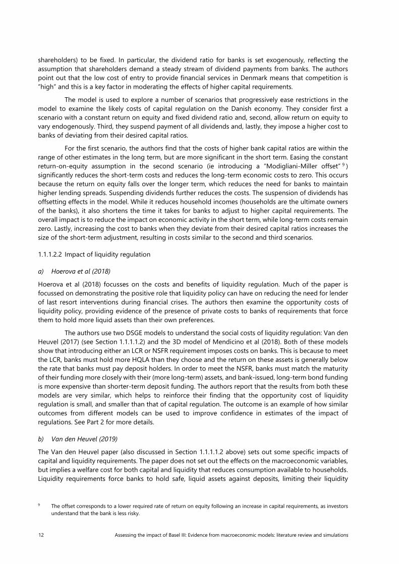
In contrast to DSGE models, there is less emphasis on the identification of the underlying channels. These models vary in complexity and use both structural and non-structural approaches to analyse the impact of regulation on the financial sector and economic activity more broadly. Some models mix the two approaches, by inserting a general equilibrium financial block into a more standard macro model. The models encompass general equilibrium outcomes as well as sectoral outcomes that can be included in a block recursive manner into larger general equilibrium models. Table 3 below sets out the papers summarised in this section.
Empirical macro models: type and policies considered Table 3
Paper Model type Policy considered
Gambacorta (2011) Vector Error Correction Capital/liquidity
de-Ramon and Straughan (2017) Vector Error Correction Capital
Conti et al (2018) Bayesian VAR Capital
Kockerols, Kravik and Mimir (2021) (Central Bank of Norway’s NEMO model)
Markov-switching crisis model and Core DSGE Capital
1.1.2.1 Vector Error Correction models with a banking sector
A number of papers develop vector error correction (VEC) models to examine the response of the economy to changes in the banking sector. In this approach, a reduced form of the banking sector is developed driven by variables more directly reflecting regulatory requirements. Another advantage of this approach is that it contains both a VAR element, which allows for examination of short-term dynamics, and an error-correction element, which describes convergence with an estimated long-run equilibrium.

14 Assessing the impact of Basel III: Evidence from macroeconomic models: literature review and simulations
a) Gambacorta (2011)
The seminal work in this area is Gambacorta (2011). The author uses the VEC framework to analyse the impact of both capital and liquidity standards on US economic activity. The estimated VEC model includes (reduced form) long-term structural relationships between variables representing the balance sheet structure of the aggregate banking sector (including the aggregate risk-based capital and liquidity (liquid assets to deposits) ratios, total lending and a measure of banks’ credit quality conditions), interest rates and equity returns (short-term real interest rates, bank lending spreads and return on bank equity) and economic activity (GDP and government expenditure). The paper identifies all variables as being endogenous within the system. Short-term dynamics are also estimated across all endogenous variables, allowing for a temporal analysis of the impact.
The author identifies four relationships that set out the long-term structural relationships between the real economy, financial markets generally and the banking sector. The first relationship sets out the bank-lending channel in which bank lending spreads are determined by the level of banks’ risk-based capital and liquidity ratios (higher regulatory requirements translate into higher spreads, as the model assumes an imperfect Modigliani-Miller effect, 10 and no effect on other components of bank funding11). The second corresponds to equilibrium output in the economy in the presence of credit markets, where total output (GDP) is determined by bank lending spreads, short-term interest rates and (exogenously determined) government expenditure. The third relationship represents demand in financial markets, with lending to the private sector determined by GDP and bank lending spreads. The fourth relationship shows bank profits, which depends on the proportion of lending in the economy and bank lending spreads.
The model uses a relatively small number of variables to represent the US economy, and it has a relatively straightforward structure. That said, the included variables allow the author to analyse the cost to economic output of both capital and liquidity regulation, which are introduced as an exogenous shock to bank balance sheets. The paper sets out a matrix of policy scenarios involving increases in risk-based capital ratios12 of 0 to 6 percentage points and increases in liquidity ratios13 of 25 and 50%.
The model confirms the standard results from the bank lending channel hypothesis: higher capital and liquidity ratios increase bank funding costs, which they recover via an increase in bank lending spreads. The analysis also confirms earlier findings that the cost of higher bank liquidity ratios has a relatively smaller effect on economic activity than increases in capital ratios. However, the modelled relationship between bank capital and liquidity is relatively simple as both elements were just linear components of bank lending spreads. Moreover, the results are sensitive to the measure of liquidity used.
In addition, the analysis shows that the increase in bank input costs driven by higher regulatory ratios lowers bank profitability, suggesting that there is a degree of competition between the banking sector and other sources of finance. Examining the dynamics of the model, the author shows that bank lending spreads adjust relatively quickly in the short term, but that bank profits adjust more slowly to the new long-term equilibrium.
Overall, the increases in capital and liquidity ratios analysed result in a relatively modest reduction in economic activity. The long-run outcome from this model is very similar to that of the Basel Committee’s analysis at that time (see MAG (2010), BCBS (2010)).
10 The Modigliani-Miller effect referred to here is the outcome, under particular conditions, that average funding costs are
invariant to the degree of leverage on banks’ balance sheets. 11 This assumption is relaxed in Gambacorta and Shin (2018). 12 Tangible Common Equity/RWA. 13 Sum of cash, government securities and net interbank lending over total deposits.

Assessing the impact of Basel III: Evidence from macroeconomic models: literature review and simulations 15
b) De-Ramon and Straughan
De-Ramon and Straughan (2017) also use a VEC approach to investigate the long- and short-term implications of higher capital ratios on the UK financial sector. In this case, the authors use the VEC framework to estimate a more detailed model of the UK banking sector (distinguishing between households and firms) than Gambacorta (2011) did using the bank-lending channel.
The key hypothesis in the model is that banks apply different lending spreads to households and PNFCs as the underlying credit risk in these sectors differs. When changing their risk-based capital ratios in the short term, it is more efficient for banks to adjust loans with a higher risk weight as this has a greater effect on risk-weighted assets. Changes in banking capital ratios may therefore affect the lending spreads to these two sectors differently. However, as banks’ funding is fungible and they cross-subsidise across their balance sheets, the difference in sector lending spreads may only be a short-term phenomenon.
The estimated VEC model bears out this hypothesis showing that, in response to an increase in bank capital ratios, banks increase lending spreads to PNFCs to a much greater extent than for households, but that there is no evidence of any difference in lending spreads over the longer term, which increase in both sectors. The long-term outcome is consistent with other general equilibrium models that use a single, aggregate lending spread for the banking sector, but suggests that the short-term dynamics may not be appropriately captured in these models.
In developing this approach, the authors show that the key endogenous variables in the model for the UK banking sector – PNFC and household lending spreads, and the risk-based capital ratio – can be modelled separately from the broader economy. Other variables included in the model (such as corporate insolvencies and unemployment) were found to be (weakly) exogenous, such that the exogenous variables can influence the long-run level of the endogenous variables, but not vice versa. Consequently, the VEC model of the banking sector can be included in a macroeconomic model in a block-recursive way. The authors used a large-scale macroeconomic model (NiGEM14) to estimate the costs to the UK economy of increases in capital ratios corresponding to estimates of the likely increase in bank capital ratios required by Basel III. As with Gambacorta (2011), the long-run impact on overall economic output (GDP) is not large, but the short-term dynamics show substantial variance in the effect on households and PNFCs.
1.1.2.2 Non-structural models including banking variables
a) Conti et al (2018)
Conti et al (2018) take a different approach to estimating the macroeconomic implications of supervisory expectations, which is more related to the literature on the impact of unconventional monetary policy measures. The authors use a non-structural Bayesian VAR for the Italian economy that includes a large number of banking sector variables, including the amount and cost of lending, default rates, bank income, bank capital and stock prices, as well as other variables reflecting overall economic activity. They note that the large number of banking-sector variables that can be included in the analysis is a key feature of the model. This allows for an endogenous characterisation of the banking sector within a broader economic context.
The model is used to isolate the impact of regulatory and supervisory shocks on bank capital from other shocks using the positive short-run forecasting properties of the BVAR approach. The other shocks to bank capital reflect other developments in the real economy and financial and credit markets. The key difference with other approaches is that regulatory shocks are measured as the standard deviation
14 NiGEM is the National Institute for Economic and Social Research (NIESR) integrated General Equilibrium Model.
See de-Ramon and Straughan (2017) and Appendix 1 of Barrell et al (2009) for a more detailed description of NiGEM.
16 Assessing the impact of Basel III: Evidence from macroeconomic models: literature review and simulations
of innovations to the capital ratio; hence, they depend on its historical properties. The response of economic activity to such shocks is then provided by the average (multivariate) correlation between the shocks and the macroeconomic variables over the sample period considered.
The authors exploit the Bayesian VAR forecasting properties to analyse three periods during which regulatory initiatives have required banks to raise capital requirements. The three periods relate to changes in regulatory and supervisory expectations: the discussion of Basel III reforms; the EBA 2011 stress test and capital exercise; and the implementation of the European Central Bank (ECB)’s comprehensive assessment and the introduction of the Single Supervisory Mechanism. 15 The technique involves estimating the BVAR model prior to each of these windows and then computing a number of out-of-sample forecasts over each window conditional on realised values for other variables. These forecasts provide a “counterfactual” for bank capital that isolates the likely path for bank capital given shocks that affect bank capital indirectly as well as an impulse response of other variables to the bank shock.
The results suggest that the shocks to banks’ capital ratios over the periods analysed were sizeable and had effects on loan volumes, loan rates and GDP. The shocks to bank capital arising from the three episodes noted above showed increases of the capital ratio by nearly 2 percentage points over a two-year period. These shocks had a negative impact on GDP in the Italian economy of varying amounts between 0.15 and 0.25 percentage points.
1.1.2.3 Markov Switching Models with financial crisis
The model of the Central Bank of Norway (Kockerols, Kravik and Mimir (2021)) embeds its fully-fledged DSGE model NEMO into a regime-switching framework, which incorporates endogenous financial crises stemming from persistently high credit growth (based on Gerdrup et al (2017)) as well as endogenous zero lower bound (ZLB) on interest rates (similar to Aruoba et al (2018)). Crises can occur at any point in time governed by a two-state Markov process. The economy can be either in a normal state or in a crisis state. Business cycles in normal times are driven by the estimated typical shocks. Crisis times are driven by some structural changes in the banking and housing sectors, and asymmetrically large low-probability crisis shocks. Both the probability and the severity of crises are determined by five-year cumulative real household credit growth, which is found to be a robust indicator of financial vulnerabilities in Norway, predicting the downside risks to GDP (see Arbatli-Saxegaard et al (2020)). The probability of a crisis is estimated based on a sample of 20 OECD countries (see Gerdrup et al (2017)).
To provide an illustration of the output of the model, the standard deviations of the asymmetric shocks and the shifting structural parameters in the crisis state used in the current document are calibrated. They roughly reflect the macroeconomic scenario used in recent macroprudential stress-testing analyses (see Central Bank of Norway (2019)).The model is able to produce downside risks to the output gap given by the asymmetric distribution (GDP-at-risk) linked to financial conditions. In this report, we use a similar version of the model in Kockerols et al (2021) that captures the costs and benefits of different capital requirement regimes. The costs of higher capital requirements are higher credit spreads and lower output in normal times while the benefits are the reduced crisis probability and lower costs of crises. The model is explained in more detail in Annex 3.
1.1.3 Quantitative results of available simulations
Table 4 below summarises the results from which we can derive quantitative estimates of the DSGE and empirical macro models, discussed in sections 1.1.1 and 1.1.2, respectively.
15 We note that only the first of these events is solely related to the introduction of Basel III.

Assessing the impact of Basel III: Evidence from macroeconomic models: literature review and simulations 17
Many of the DSGE models reviewed in Section 1.1.1 integrate a capital channel that allows one to assess the cost of solvency regulation in terms of reduced lending. Some of them also measure the benefits. Very few of the standard quantitative DSGE models provide results on liquidity.
Of the empirical macro models, all four papers quantify the opportunity cost to the economy of changes in capital ratios, while Gambacorta includes estimates for a range of both capital ratio and liquid asset changes. These models tend to demonstrate that the overall impact of higher capital charges on economic output is limited.
Long-run impact of capital and liquidity requirements from various macroeconomic models Table 4
Paper Increase in capital and liquidity requirement
Loan level GDP level
DSGE models
De Nicolò et al (2014) Partial equilibrium
Leverage ratio at 4% and LCR at 50%
-26%
Covas and Driscol (2014) DSGE
LCR (of 100%) on top of 6% capital requirement
-3% -0.3% (from one steady state to another)
Begenau (2019) Capital ratio +3.15% pts (9.25% to 12.4%)
+2.35% +0.02%
Elenev, Landvoigt and Van Nieuwerburgh (2020)
Capital ratio +8% pts (7% to 15%)
-8% pts corporate debt/GDP
-0.21%
3D model on euro area (2020)1 +5% pts capital in five years (11.5% to 16.5%)
+2.55% +1.2%
3D model on United States (2020)1
+5% pts capital in five years (10.5% to 15.5%)
+8.03% +0.87%
de Bandt and Chahad (2016) with bank run for the euro area1
+5% pts capital in five years (11.5% to 16.5%)
+1.26% +0.2%
2020 update of Gerali et al (2010) for euro area – cost approach1
+5% pts capital in five years (11.5% to 16.5%)
-5.85% -0.4%
Central Bank of Norway’s NEMO (2020)1,2
+5% pts capital in five years (11.3% to 16.3%)
-3.18% (12.9%) -0.2% (2.1%)
Empirical macro models (cost estimates only)
Gambacorta (2011) LCR increase of 0–50% Capital ratio +2/4/6% pts
-0.36 to -1.31% -0.19 to -0.70%
de-Ramon and Straughan (2017) Capital ratio +8% pts – -0.2%
Conti et al (2018)3 Capital ratio +1.6% pts PNFCs: -0.01% pts Households: -0.03% pts
-0.02% pts
1 See Table 7. 2 The numbers in parentheses are computed under the assumption of a higher crisis probability and severity. 3 Results show estimate of impact after two years.
1.2 Alternative modelling approaches (mostly stylised/qualitative models)
In this section, we consider developments in alternative models to shed some light on possible improvements that could be made to the existing macro models reviewed in Section 1.1. We focus on recent contributions concerning the modelling of financial crises (and thereby the benefits of banking regulation) (Section 1.2.1), models including a shadow banking sector (Section 1.2.2) and modelling the effects of other kinds of regulation beyond the core regulations on capital and liquidity (Section 1.2.3).

18 Assessing the impact of Basel III: Evidence from macroeconomic models: literature review and simulations
1.2.1 Modelling financial crises and the benefits of banking regulation
The standard DSGE models in their original nonlinear form are subject to very complex dynamics. Since an analysis of the complete nonlinear dynamics is computationally very burdensome (to the point of not being feasible in reasonable time if the model is rich enough for policy analysis), the standard approach in the literature is to linearise the model around a steady state. Economic fluctuations are analysed in terms of small deviations from that steady state. This approach is useful to analyse policy in normal times, but insufficient if one wants to analyse a policy during times of crisis.
Basel III policies, however, were explicitly introduced to reduce the probability of a crisis and mitigate the negative effects of a crisis. To measure the benefits of Basel III regulation, especially liquidity regulation, in a comprehensive way it is therefore necessary to extend standard models to incorporate an endogenous crisis which can potentially be mitigated or prevented in some cases by the policies. The need for liquidity regulation, for instance, arises for several reasons. First, there may be a risk of unexpected withdrawal of depositors or other funding (due to loss of confidence during a financial crisis). Second, there may be a market failure in the sense that banks do not by themselves hold enough liquid assets (see Mordel (2018) for a literature survey on prudential liquidity regulation in banking). Such a liquidity crisis can arise, for example, because of a loss of confidence on the interbank market, the money market or other short-term funding markets.
In the following, we therefore review models that incorporate an endogenous financial crisis. A financial crisis arises when shocks to financial markets spill over to the real economy through the following channels:
• net worth/occasionally binding intermediary funding constraints;
• pecuniary externalities16 (with ensuing fire sale dynamics)/collateral channel;
• savings gluts and boom-bust cycle dynamics; and
• coordination failure and strategic complementarity (bank runs).
Table 5 shows a categorisation of the models surveyed in Section 1.2.1 according to the channels that are active.
Alternative modelling approaches by channels of transmission Table 5
Channels Papers
Net worth/occasionally binding intermediary funding constraints
Brunnermeier and Sannikov (2014); He and Krishnamurthy (2019); Holden, Levine and Swarbrick (2019); Schroth (2021); Elenev, Landvoigt and Van Nieuwerburgh (2020)
Pecuniary externalities/collateral channel Mendoza and Smith (2006); Mendoza (2010); Korinek and Mendoza (2014); Bianchi and Mendoza (2018); Davila and Korinek (2018); Benigno et al (2013); Korinek and Simsek (2016); Jeanne and Korinek (2019); Jeanne and Korinek (2020); Walther (2016); Ikeda (2018)
Savings gluts and boom-bust cycle dynamics
Boissay, Collard and Smets (2016); Martinez-Miera and Repullo (2017); Swarbrick (2019); Kockerols, Kravik and Mimir (2021) (Central Bank of Norway’s Model – NEMO), Coimbra and Rey (2020)
Coordination failure and strategic complementarity (bank runs)
Kashyap, Tsomocos and Vardoulakis(2020); Miller and Sowerbutts (2018); Gertler and Kiyotaki (2015); Gertler, Kiyotaki and Prestipino (2019)
16 A pecuniary externality is an externality which operates through prices (here, asset prices) rather than through real resource
effects.
Assessing the impact of Basel III: Evidence from macroeconomic models: literature review and simulations 19
1.2.1.1 Further modelling of occasionally binding intermediary funding constraints
In Section 1.1.1.1.1 we reviewed models where the level of bank net worth determines the probability that the bank becomes funding constrained as a result of (possibly small) exogenous shocks. We present here some alternative models to the standard DSGE models presented earlier which go further in terms of studying full dynamics (Brunnermeier and Sannikov (2014), He and Krishnamurthy (2019)) or cyclical properties (Holden et al (2019), Schroth (2021)).
(a) Brunnermeier and Sannikov (2014)
Brunnermeier and Sannikov (2014) is one of the first papers to study a DSGE model with financial frictions in its full dynamics, ie going beyond analysing the local effects around the steady state. In their model economy, the efficient experts (banks) manage capital very productively in contrast to the less efficient households. The financial friction consists in the assumption that productive agents cannot issue as much equity as they want (ideally, they would take over the whole production process and households would just own their equity). To finance more productive operations the experts borrow funds from the households at the risk-free rate (leverage themselves) since they cannot issue more equity by assumption. The resulting equilibrium then features inefficiencies compared to a frictionless economy, in particular, capital is misallocated, there is underinvestment and consumption is distorted. Furthermore, this set-up leads to interesting dynamic properties: the system is relatively stable near to the steady state (normal times), but can exhibit instability once it is sufficiently far away from the steady state (crisis times).
The authors quantitatively analyse the effect of capital requirements (leverage constraint) in their framework by providing a numerical example. According to their analysis, leverage constraints do not improve welfare in most constellations since the output costs outweigh the benefit of stabilising the system. Those results should be taken with caution however since the model is stylised and it is not calibrated to match real data.
(b) He and Krishnamurthy (2019)
He and Krishnamurthy (2019) analyse a model of a more quantitative nature, which can be calibrated to match real data. In their model intermediaries (banks, hedge funds or broker/dealers) derive utility from their equity directly, interpreted as their “reputation”. The authors’ idea is to introduce funding constraints and funding shocks similar to the situation of intermediaries during a financial crisis where funding becomes more difficult due to loss of confidence in the markets. More specifically, the intermediaries can only raise a limited amount of equity (up to a certain amount, raising equity is possible at zero cost but beyond this amount it becomes too expensive to raise more – the cost is effectively infinite). The amount of equity which can be raised (equity capital capacity of the intermediary) depends on the return on equity which is subject to shocks (the funding shocks). The resulting dynamics of equity capital capacity resemble very closely the dynamics of “net worth” in other models described in this report (eg the model by Brunnermeier and Sannikov (2014) described above in this section).
The model’s equilibrium is a stochastic steady state distribution for the economy, in which systemic states, ie where constraints on the financial sector bind, correspond to only some of the possible realisations of the state variables. Moreover, in any given state, agents anticipate that future shocks may lead to constraints tightening, triggering systemic risk. As the economy moves closer to a systemic state, these anticipation effects cause banks to reduce lending and hence investment falls even though capital constraints are not binding. When constraints on the intermediary sector are binding or likely to bind in the near future, a negative funding shock triggers a substantial decline in intermediary equity, asset prices and investment. When constraints on the intermediary sector are slack and unlikely to bind in the near future, the same size negative shock triggers only a small decline in intermediary equity, asset prices and investment. In short, the model generates conditional amplification, where the state variable determining conditionality is the incidence of financial constraints in the intermediary sector.
20 Assessing the impact of Basel III: Evidence from macroeconomic models: literature review and simulations
In terms of policy analysis, the authors show how their model can be used to conduct a macroeconomic “stress test” linking a stress scenario to the probability of systemic risk states. Their stress test scenarios indicate that, if bank equity suffers a loss of 5%, the probability of a crisis within the next two years rises modestly to 19.2%. But a 25% loss on bank equity pushes the economy into the crisis state, and this is why with probability 100% there will be a crisis in the next two years.
(c) Holden, Levine and Swarbrick (2019)
Holden, Levine and Swarbrick (2019) study the joint cyclicality of bank debt and equity issuance under occasionally binding financial constraints, analysing the impact of financial constraints on macroeconomic time series and the presence of occasional credit crunches. In contrast to the models by Brunnermeier and Sannikov (2014) and by He and Krishnamurthy (2019) the occasionally binding constraint is not assumed on bank equity but on bank debt. The authors argue that this is more in line with what is empirically observed during credit crunches, in particular the fact that intermediaries tend to increase their equity issuance rather than reduce it during credit crunches. The model can thus help interpret the joint cyclical dynamics of bank debt and equity finance observed in the data in a more consistent way. Under normal circumstances, banks rely on debt finance. However, under financial stress, borrowing constraints can bind and if the conditions are bad enough, banks must raise additional equity finance at cost. This results in occasional episodes with sharp increases in spreads and deeper downturns, helping explain observed macroeconomic asymmetries such as negatively skewed aggregate investment.
(d) Elenev, Landvoigt and Van Nieuwerburgh (2020)
Elenev et al (2020) develop a general equilibrium model, where financial crises arise endogenously. The model is solved non-linearly like Brunnermeier and Sannikov (2014) and He and Krishnamurty (2013). They study the impact of increasing the minimum bank equity capital requirement from its pre-crisis level of 7% of assets. Higher capital requirements are successful at reducing financial leverage and the bank failure rate. But the size of the economy decreases. Macroeconomic volatility declines, reflecting the balance of two forces. A smaller banking sector has less risk absorption capacity, raising volatility, but the reduced financial fragility lowers volatility. According to their analysis, pre-crisis capital requirements in the United States were close to optimal in terms of aggregate welfare of savers and borrowers. The model captures the sharp and persistent drop in macroeconomic aggregates and credit provision as well as the sharp change in credit spreads observed during the Great Recession. In a financial crisis, intermediaries contract the size of their balance sheet, reducing the supply of safe assets. The reduction in the supply of deposits is offset by an increase in government debt due to counter-cyclical fiscal policy and bank bailouts. Demand for safe assets increases due to a precautionary demand. The net effect is lower interest rates in a crisis. From the methodological point of view, the paper introduces a method to solve a model with two exogenous and persistent sources of aggregate risk and five endogenous aggregate state variables which track the wealth distribution. It features default and occasionally binding borrowing constraints in both non-financial and financial sectors.
(e) Schroth (2021)
Schroth (2021) uses a model with occasionally binding intermediary funding constraints to discuss the implementation of the capital conservation buffer and the countercyclical capital buffer (CCyB). The analysis emphasises that regulatory capital buffers are about restricting bank equity payouts rather than bank lending over financial cycles (for more details on the results see below in the section on “macroprudential policies”).
The focus of most of the contributions presented in this section is the analysis of capital requirements. Modelling elements to analyse liquidity regulation are missing. Some of the contributions discussed in the following sections will fill this gap.

Assessing the impact of Basel III: Evidence from macroeconomic models: literature review and simulations 21
1.2.1.2 Pecuniary externalities (with ensuing fire sales dynamics)/collateral channel
Following Kiyotaki and Moore (1997) (see Section 1.1.1.1.2), pecuniary externalities arise when agents’ price taking behaviour fails to internalise the feedback mechanism from collateral price changes, accelerating fire sales. The consequence is over-borrowing relative to a constrained-optimal allocation that internalises this effect. Relative to the social optimum, crises happen more frequently in an unregulated economy with over-borrowing since collateral constraints are more likely to bind as the amount of debt to be rolled over increases.17 Moreover, conditional on entering a crisis, the magnitude of a disaster tends to be larger since agents need to fire-sell more assets for consumption smoothing and that leads to a larger decline in the price of collateral, which further tightens collateral constraints. In this economy, an ex ante macroprudential regulation can help reduce a build-up of debt and reduce occurrences and the severity of crises.
In this subsection, we present a part of the literature, which studies more in depth economies under pecuniary externalities. Some of the papers presented in this section do not include Basel III policies explicitly (Mendoza and Smith (2006), Mendoza (2010), Korinek and Mendoza (2014), Davila and Korinek (2018)). Benigno et al (2013) and Bianchi and Mendoza (2018) include results on macroprudential policy. Other contributions using models with pecuniary externalities to analyse macroprudential policies are Korinek and Simsek (2016), Jeanne and Korinek (2019) and Jeanne and Korinek (2020) (see section below on macroprudential policies). Walther (2016) and Ikeda (2018) consider explicitly capital and liquidity regulation.
(a) Mendoza and Smith (2006), Mendoza (2010), Korinek and Mendoza (2014), Bianchi and Mendoza (2018)
A suite of papers by Mendoza and co-authors study pecuniary externalities in the context of sudden stops.18 These four papers build on Fisher’s debt deflation mechanism. When leverage is elevated, adverse shocks of standard size can trigger the collateral constraint. Agents thus sell their assets to meet the collateral constraint, which causes a drop in asset prices and triggers Fisher’s debt deflation mechanism. Indeed, as asset prices collapse, agents are forced to sell more assets to comply with the collateral constraint, which amplifies the initial impact of the shock. Moreover, these fire sales are not enough to satisfy the collateral constraint, and agents reduce consumption and/or investment. All these papers demonstrate that financial crises are rare and extreme events triggered by small-sized shocks when leverage is high. Bianchi and Mendoza (2018) analyse macroprudential policies in such a set-up with pecuniary externalities (see the section on macroprudential policies below). However, none of these papers takes into account explicitly capital and liquidity regulation.
(b) Davila and Korinek (2018)
In an interesting theoretical contribution, Davila and Korinek (2018) distinguish two types of pecuniary externalities: distributive and collateral. The former arises when marginal rates of substitution (MRS) between dates/states differ across agents, and a planner can improve upon the allocation by affecting relative prices at which the agents trade. The latter is the same channel as described by Kiyotaki and Moore (1997). Whereas the collateral externalities lead to over-borrowing, the effect of distributive externalities is ambiguous.
A regulator who wants to correct distributive externalities (when MRS are not equal across economic agents) can modify allocations by inducing price changes that improve the terms of the transactions of those agents with relatively higher marginal utility in a given date/state. Moreover, a
17 A crisis is defined as a state in which consumption declines by more than two-standard deviations of the steady-state value.
18 A sudden stop is a reversal in private capital flows into emerging market economies and a corresponding sharp reversal from large current account deficits into smaller deficits or small surpluses.

22 Assessing the impact of Basel III: Evidence from macroeconomic models: literature review and simulations
planner who wants to mitigate collateral externalities can attempt to reduce the likelihood and effects of fire sales to raise the value of capital assets that serve as collateral, which relaxes financial constraints. The authors stress this point in a specific application of their general model. Assuming a specific utility function for the borrowers and a specific technology of lenders, they show that, in this framework, the collateral externalities lead to over-borrowing in equilibrium. A qualitative policy conclusion from this application is consequently that it is desirable to shore up the net worth of agents determining the relevant asset prices for collateral, either by inducing them to buy insurance against bad states or, in the absence of such insurance markets, by restricting their borrowing. Furthermore, it is desirable to intervene in the investment decisions of these agents to mitigate price declines (restrict investment in assets that drain liquidity in a crisis and encourage investment in assets that provide additional liquidity also in times of crisis).
Their model thus yields interesting theoretical qualitative insights on two types of pecuniary externalities (distributive and collateral). However, it is highly stylised and cannot be used directly for quantitative policy analysis.
(c) Benigno et al (2013)
Benigno et al (2013) draw on Mendoza (2010) with a focus on macroprudential policy. In the decentralised equilibrium, agents do not internalise the effect of their borrowing decision on the probability that the constraint becomes binding (pecuniary externality). Thus, the social planner values savings more than private agents in the decentralised equilibrium and should therefore limit credit. Apart from the pecuniary externality there is, however, also a crisis management effect: if by assumption the social planner can efficiently manipulate the resource allocation ex post, this crisis management mitigates the effect of the crisis when it occurs as well as its probability of occurrence and changes fundamentally the properties of the equilibrium. In fact, this possibility for ex post crisis management lowers the value of savings compared to the decentralised equilibrium.
Intuitively, if the expectation is that the social planner will mitigate the crisis ex post and also, thereby, reduce the probability of a crisis, it is inefficient for the agents to insure themselves intensively against such a crisis by accumulating a lot of savings. The authors argue that it is likely that the effect of the possibility of ex post crisis management (crisis management effect) dominates the effect of the pecuniary externality. Thus, the decentralised equilibrium features under-borrowing compared to the optimal social planner allocation. Again, capital and liquidity regulation is not discussed explicitly (see section below for more details on the results concerning macroprudential policies).
(d) Walther (2016)
Walther (2016) presents a three-period model of an economy with financial frictions to analyse macroprudential regulation and its interaction with microprudential regulation. In this framework, banks face three different kinds of frictions: First, the banks need equity downpayments (“skin in the game”) to raise funding. Second, banks can only sell assets to outsiders at fire sale prices which is assumed to be socially wasteful as outsiders cannot extract as much surplus from assets as banks (ie similar to the pecuniary externalities described above). Third, banks’ creditors have a preference for liquidity, so that long-term debt commands an interest premium. Thus, similar to the other papers in this section, there is the problem of socially wasteful fire sales leading to an inefficient equilibrium without regulation. The novelty of this paper is that on top of that by assuming a liquidity premium the model allows one to study the interplay between the endogenous maturity structure of banks and fire sales.
In a first step, the author characterises the optimal macroprudential policy in his framework. Without regulation, banks choose excessive leverage and maturity mismatch in equilibrium, as they fail to internalise the risk of socially wasteful fire sales. Three different policies are considered to address this inefficiency: centralisation, balance sheet constraints or Pigouvian. The policy of balance sheet constraints is the most favourable in practical terms since it requires less information by the planner. The author then

Assessing the impact of Basel III: Evidence from macroeconomic models: literature review and simulations 23
shows that such an optimal policy can be implemented within the Basel III framework using either the LCR or the NSFR.
In a second step, the goal is to analyse the interaction of macroprudential and microprudential policies. To do this he extends his framework by introducing socially wasteful bank defaults. The author shows that in such a framework where the regulator needs to protect the economy from socially wasteful fire sales as well as socially wasteful bank defaults macro- and microprudential policies are substitutable, but not necessarily perfect substitutes depending on the parameter values. If bad individual shocks are sufficiently severe, then microprudential policy needs to be very tough to rule out individual defaults. In this case, regardless of banks’ maturity mismatch, their choices always satisfy the no-fire-sale condition and an additional macroprudential constraint is not required. If bad individual shocks are not severe, both a micro- and a macroprudential policy are needed. Although the macroprudential constraint on bank leverage prevents the default of banks with adverse individual shocks to some extent it can never rule out default in general.
(e) Ikeda (2018)
Ikeda (2018) presents a two- (or three-) period model of bank runs with a special form of pecuniary externality. There are three types of agents: households, fund managers and banks. In the first period, households deposit part of their endowment in a bank, but delegate the management of their deposit to fund managers who are assumed to have information advantages. In the second period, the bank either defaults and the household obtains only the recovery value of the deposit or the bank does not default and the household obtains the full value of the deposit including interest payments. The fund managers obtain a noisy signal about a risky investment of the banks. If the signal is below some threshold, the fund managers’ strategy in this game is to withdraw the funds early at the beginning of the second period. The banks invest their net worth and the deposits in a risky project in the first period. Bank leverage is defined by total assets (net worth and deposits) divided by equity (net worth). In the second period, the banks may face an early liquidation before the return on the risky project is realised and need to liquidate some of their assets at costly losses. In an extended version of the baseline model, the bank also faces the choice of investing in a safe technology (liquid assets) with a lower return than the risky assets.
In the equilibrium of this model, there is the following effect similar to the pecuniary externalities described in the other models of this section: the leverage and liquidity of one individual bank affects the threshold that a fund manager sets for all banks for the noisy signal about the return on the risky investment. The individual bank fails to internalise the negative effect its individual decision on leverage and liquidity has on the whole market. This induces excessive leverage and insufficient liquidity, resulting in higher systemic risk. When a crisis occurs, banks use liquidity first because doing so is not costly. Then, if the amount of liquidity is not enough to cover the amount of the claim, they start to sell their risky assets at a fire-sale price. Jointly optimal requirements on both leverage and liquidity can differ significantly depending on parameter values, in particular the parameter that characterises the supply side of funds.
1.2.1.3 Savings gluts and boom-bust cycle dynamics
Empirical studies find that credit is not only depressed during and following a financial crisis but is also often elevated prior to financial crises (Schularick and Taylor (2012)). A number of theoretical papers have proposed channels that can explain a causal link between high credit ex ante and the occurrence of a financial crisis ex post. Many of these channels rely on some form of domestic savings glut argument (Bernanke (2005)) and are likely also present when there is an international savings glut. The savings glut lowers the interest rate and induces more risky lending such that a financial crisis becomes more likely. There is additional feedback because the financial instability created by a savings glut further increases the incentive to save and to bid up asset prices.

24 Assessing the impact of Basel III: Evidence from macroeconomic models: literature review and simulations
(a) Boissay, Collard and Smets (2016)
In the modelling environment of Boissay, Collard and Smets (2016), the end of an economic boom creates a mismatch between high supply of savings (ie wealth created during the boom) and few productive investment opportunities. The resulting fall in the interbank interest rate induces banks with low intermediation ability to lend their funds directly to firms (final borrowers) rather than supplying them to more able banks through the interbank market. Bank abilities are not observable by lenders on the interbank market. As the average ability of borrowers in the interbank market falls, each borrower obtains fewer funds. This process might continue until the interbank market freezes at which point credit supply drops. During the “credit boom”, the credit to output ratio increases sharply while consumption and investment decrease (because the economic boom has ended). A boom could be ended through a shock to commodity prices or trade relationships.
(b) Martinez-Miera and Repullo (2017)
Martinez-Miera and Repullo (2017) present a model in which a credit boom begins during an economic boom. When wealth is high enough, savers prefer to put more savings aside in case the economic boom ends in a financial crisis. This leads to decreasing returns to physical capital beyond what one would expect in terms of a standard response of returns during the business cycle. Interest rates are in turn overly depressed and lending spreads excessively low. In this situation, banks optimally choose to monitor less, since monitoring is costly and their profit is lower due to lower lending spreads. Borrowers become riskier as a consequence and a crisis then becomes endogenously more likely.
(c) Swarbrick (2019)
In a similar spirit, Swarbrick (2019) highlights how low interest rates increase the risk of a credit crunch in a theoretical DSGE model with asymmetric information about the types of small businesses (borrowers). The borrowers know their type, but the lenders do not know it leading to adverse selection and credit rationing. When riskier firms have a higher return, when successful, then banks can offer loan contracts with different terms set so that the risky and safe firms choose the contract designed for them. Risky firms will choose a loan with higher interest rates if it offers a higher loan approval rating than safe loans because they would be more likely to be denied credit if choosing a safe loan with a low interest rate and lower approval.
Safe borrowers will choose the safe loan since this is the only type of loan that they can repay. The author also finds that when the risk of default increases enough, as it did during the recent crisis, banks do not lend all available funds and restrict credit to safe firms. This rationing of credit causes a fall in productivity because there is a drop in the available capital being utilised in production. Furthermore, the author shows that the risk of such a credit crunch is heightened and economic fluctuations are amplified when real returns on capital are sufficiently low.
(d) Coimbra and Rey (2020)
Coimbra and Rey (2020) focus on the effect of low interest rates on aggregate risk-taking and the probability of a financial crisis. In their model, regulation is in the form of a value-at-risk constraint (which is a market-based, risk-weighted solvency ratio) that limits the probability of default of intermediaries. The model assumes a distribution in the tightness of this constraint across a continuum of financial intermediaries and changes in regulation can be seen as shifts in this distribution. Such an assumption may be justified by a homogeneous regulation applied to different business models. Given there is an option value of default, riskier intermediaries will have a higher willingness to pay for risky financial assets and competition can price out some of the safer intermediaries from risky capital markets. Moreover, the authors show that the leverage of riskier intermediaries is more elastic with respect to the cost of funds than that of safer ones.

Assessing the impact of Basel III: Evidence from macroeconomic models: literature review and simulations 25
When the cost of funds becomes low, risky intermediaries are able to lever up more and aggregate risk-taking grows because of a selection effect (fewer safe intermediaries holding risky assets due to increased competition) and a composition effect (a larger share of assets being held by more risk-taking ones). These two effects imply that leverage booms driven by cheap access to funds increase the probability of large-scale bank defaults. Moreover, the selection effect implies that the marginal investor is now more risk-taking, so the equity premium is also lower during such booms. Although the authors do not explore the effects of a time-varying regulation, they show through comparative statics that tighter regulation can reduce the frequency of such crises, but at a cost of lower investment and output during normal periods.
1.2.1.4 Coordination failure and strategic complementarity (bank runs)
A theoretical approach suitable for studying crisis phenomena (including bank runs, debt crises and currency attacks) are global coordination games of regime change. Agents take an action (withdraw deposits from a bank, refuse to roll over short-term debt, or attack a fixed exchange rate regime of a currency) and their incentive to act increases in the proportion of agents acting (strategic complementarity). A classic example is the Diamond and Dybvig (1983) bank-run model.
In the following, we present, first, three-period models extending the Diamond and Dybvig framework to be able to draw some interesting policy conclusions (Miller and Sowerbutts (2018), Kashyap et al (2020)). Then, we discuss contributions going beyond three-period frameworks by investigating infinite horizon DSGE models with financial accelerator effects and bank runs (Gertler and Kiyotaki (2015), Gertler et al (2019)).
(a) Miller and Sowerbutts (2018)
Miller and Sowerbutts (2018) create a model that endogenises banks’ funding costs to include their liquidity management. It is a three-period model with two agents: a representative bank and a continuum of investors. Banks’ liabilities are uninsured short-term debt and equity, and the bank optimises profits over assets consisting of cash and loans. The model assumes that the return on loans is common knowledge, so the sole role of banks is liquidity transformation and the impact of liquidity policy is highlighted. Investors provide debt funding from which they receive the returns made by the bank. Investors have the option of withdrawing their debt funding in the second period (early withdrawal) if they think returns will not materialise (based on private information).
The model allows for endogenous bank runs. The central bank runs a committed facility and lends at a haircut. Banks can borrow to meet any withdrawals, but subject to the central bank knowing the quality of the banks’ lending. The model shows that solvent banks may become subject to runs because of lack of liquidity. A social planner can choose a level of liquid assets that effectively eliminates the likelihood of bank failure due to illiquidity (the bank can still fail because of insolvency). However, the outcome is not supported in any equilibrium: banks will always choose to accept some liquidity risk. Requiring banks to hold higher levels of liquid assets will reduce bank profits by reducing asset returns, but the bank is less subject to runs so part of the reduction in asset returns reflects the lower level of liquidity risk. The same kind of model where liquidity regulation reduces banks’ profits but also the probability of bank runs is developed by Hoerova et al (2018), as well as de Bandt et al (2021).
(b) Kashyap, Tsomocos and Vardoulakis (2020)
Kashyap, Tsomocos and Vardoulakis (2020) present a three-period model with liquidity shocks and bank runs à la Diamond and Dybvig, but modified so that, besides offering liquidity services to depositors, banks also raise equity funding, make loans that are risky and invest in safe, liquid assets. The bank and its borrowers are subject to limited liability. When profitable, banks monitor borrowers to ensure that they repay loans. Depositors may choose to run based on conjectures about the resources that are available for people withdrawing early and beliefs about banks’ monitoring.

26 Assessing the impact of Basel III: Evidence from macroeconomic models: literature review and simulations
The authors use a new type of global game to solve for the run decision. They find that banks opt for a more deposit-intensive capital structure than a social planner would choose. The privately chosen asset portfolio can be more or less lending-intensive, while the scale of intermediation can also be higher or lower depending on a planner’s preferences between liquidity provision and credit extension. To correct the three distortions associated with the bank’s asset allocation, capital structure and scale of intermediation, a package of three regulations is warranted. The asset and liability distortions can be corrected using a capital and a liquidity requirement. Capital and liquidity requirements are jointly helpful and should be treated as complementary, since they operate on different intermediation margins. However, both are less effective at boosting the overall scale of intermediation, which the planner may favour in order to expand lending and help borrowers. To raise or lower the scale of intermediation, other regulations, such as deposit subsidies or lending subsidies, would be needed.
(c) Gertler and Kiyotaki (2015)
According to Gertler and Kiyotaki (2015), a recession that constrains bank lending due to conventional financial accelerator effects can also raise the possibility of runs due to the associated weakening of balance sheets and reduced liquidity of secondary markets for bank assets. The existence of a bank run depends on two factors: the condition of bank balance sheets and an endogenously determined asset liquidation price. A banking crisis induces banks to sell their assets to households, leading to a drop in asset prices. The severity of the drop in asset prices depends on the quantity of sales and the efficiency of households in managing capital (who are generally less efficient than banks). Two equilibria might exist: a no-run equilibrium where households roll over their deposits in banks; and a run equilibrium where households stop rolling over their deposits, banks are liquidated and households use their residual funds to acquire capital directly.
An increase in the perceived likelihood of a bank run has harmful effects on the economy even if a bank run does not materialise. It does so by causing bank credit to contract, partly by reducing the maximum leverage ratio and partly by causing aggregate net worth to shrink due to an increased deposit rate. Moreover, the dependency of the bank run probability on the recovery rate works to amplify the effects of aggregate disturbances to the economy, even beyond the amplification that originates from the conventional financial accelerator.
In response to a 5% decline in productivity, output, bank lending and bank net worth fall by 6%, 25% and 50%, respectively, in the model with no bank runs. Credit spreads increase by 70 basis points in annualised terms and asset prices decline by 5.5%. In the equilibrium with a positive probability of run, in response to a 5% decline in productivity, the probability of a run increases to 2% per quarter on impact. Output, bank lending and bank net worth fall by about 7%, 50% and 80%, respectively. Credit spreads increase by 145 basis points in annualised terms and asset prices decline by 8%.
The paper qualitatively considers the imposition of capital requirements via setting a regulatory minimum for the leverage ratio that is above the “laissez-faire” value. Individual banks do not take into account the effect of their leverage decisions on the extent of asset fire sales in distressed times, leading to excessive leverage (leverage ratios that are too low) in the competitive equilibrium. Moreover, given the link between the leverage ratio and the probability of runs, capital requirements that raise the leverage ratio reduce the probability of runs. However, there is a clear trade-off in implementing this policy. The trade-off stems from the fact that while tighter capital requirements may reduce the probability of runs, they also reduce the level of financial intermediation. This leads to lower real economic activity by increasing the cost of capital. The paper argues that the socially optimal leverage ratio should lie above its “laissez-faire” value but it should be countercyclical. A fixed regulatory capital requirement may generate an excessive fall in bank lending during an economic downturn.

Assessing the impact of Basel III: Evidence from macroeconomic models: literature review and simulations 27
(d) Gertler, Kiyotaki and Prestipino (2019)
Gertler, Kiyotaki and Prestipino (2019) characterise bank runs as self-fulfilling rollover crises, following the Calvo (1988) and Cole and Kehoe (2000) models of sovereign debt crises and emphasise the complementary nature of balance sheet conditions and bank runs. A panic or run in the model is a self-fulfilling failure of creditors to roll over their short-term credits to banks. Balance sheet conditions affect not only borrower access to credit but also whether the banking system is vulnerable to a run. In this way, the model is able to capture the highly nonlinear nature of a collapse: When bank balance sheets are strong, negative shocks do not push the financial system to the verge of collapse. When they are weak, a shock of the same size leads the economy into a crisis zone in which a bank run equilibrium exists.
As an exogenous source of variation in the return on capital, the authors assume that there are shocks to the quality of capital. When the economy is close to the steady state, a self-fulfilling rollover crisis cannot happen because banks have sufficiently strong balance sheets. In this situation, "normal size" business cycle shocks do not lead to financial crises. In this context, a shock to the quality of capital reduces the expected return to capital, reducing investment and in turn aggregate demand. In addition, for the baseline economy with financial frictions, the weakening of bank balance sheets amplifies the contraction in demand through the financial accelerator or credit cycle mechanism of Bernanke et al (1999) and Kiyotaki and Moore (1997). Poor asset returns following the shock cause bank net worth to decrease. As bank net worth declines, incentive constraints tighten and banks decrease their demand for assets, causing the price of capital to drop. The drop in asset prices feeds back into lower bank net worth, an effect that is magnified by the extent of bank leverage.
However, in a recession, banks may have sufficiently weak balance sheets so as to open up the possibility of a run. Depending on the circumstances, either a small shock or no further shock can generate a run that has devastating consequences for the real economy. When the sunspot is observed and the run occurs, bank net worth is wiped out which forces banks to liquidate assets. In turn, households absorb the entire capital stock; however, households are only willing to increase their portfolio holdings of capital at a discount, which leads excess returns to spike and investment to collapse. When the run occurs, investment drops an additional 25% resulting in an overall drop of 35%.
1.2.2 Models including a shadow banking sector
The ability to include a shadow banking sector, which in the models studied is comprised of financial intermediaries that are more lightly regulated than commercial banks, is an important modelling feature that increases the relevance of these macroeconomic models for economies that rely comparatively less on banking finance. A number of recent papers presented here make the effort of explicitly including a shadow banking sector into the model (Ikeda (2018), Begenau and Landvoigt (2018), Durdu and Zhong (2019), Martinez-Miera and Repullo (2019)).
(a) Ikeda (2018)
One of the contributions already discussed above, Ikeda (2018), extends the basic model to include heterogeneous banks (regulated and unregulated banks). The author shows that as the leverage restriction on the regulated bank is tightened, the unrestricted bank, which can be interpreted as shadow banking, increases leverage and, as a result, its default probability rises.
(b) Begenau and Landvoigt (2018)
Begenau and Landvoigt (2018) present a quantitative general equilibrium (real business cycle type) model to quantify the costs and benefits of tighter bank regulation in an economy with regulated commercial banks and unregulated shadow banks. Increasing capital requirements forces the commercial banks to fund themselves in a more expensive way (by issuing equity instead of deposits). The shadow banking sector expands since it becomes relatively more profitable. The quantitative analysis shows that at the optimal level of capital for banks, estimated to be at 17% of risk-weighted assets, the increased riskiness

28 Assessing the impact of Basel III: Evidence from macroeconomic models: literature review and simulations
of shadow banks is more than offset by the greater stability of commercial banks. Said differently, although there are unintended consequences of capital regulation, until reaching the optimal level, higher capital requirements have net benefits in terms of welfare for the whole economy.
(c) Durdu and Zhong (2019)
Durdu and Zhong (2019) analyse the effects of changes in capital requirements in an empirically realistic model with a bank and non-bank sector. Raising bank capital requirements means that for each unit of lending in which banks engage more inside equity is needed. The model allows inside equity to move across firms in the financial sector, leading to equity flows. The authors find that when bank capital requirements increase, equity flows from the non-bank sector to the bank sector so that the banking sector can meet the higher capital requirement. Given the existence of these inside equity flows between banks and non-banks, the effect on bank lending growth is ambiguous, but non-bank leverage increases due to equity outflows from non-banks to banks. The probability of default in the banking sector decreases. From the estimated model, however, bank capital requirements historically have not played an important role in driving bank and non-bank lending growth dynamics. This is largely due to inside equity flows between banks and non-banks undoing any quantity effects of bank and non-bank lending. Shocks to the balance sheets of entrepreneurs who borrow from the financial sector, as well as risk shocks that affect the idiosyncratic risk of the entrepreneur investment projects, seem to be the main drivers of bank and non-bank lending growth in the United States.
(d) Martinez-Miera and Repullo (2019)
Martinez-Miera and Repullo (2019) present a two-period stylised model to analyse capital requirements in the presence of both a regulated sector and a shadow banking sector. Heterogeneous entrepreneurs differ according to their (observable) risk profile and have access to three types of funding: (i) the market; (ii) regulated banks; and (iii) shadow banks. Banks have access to a screening technology, allowing a reduction in entrepreneurs’ default probability, while the market does not have access to the screening technology. Banks are financed by investors who do not observe monitoring efforts, giving rise to an agency problem mitigated by bank’s capital (skin in the game). Banks endogenously choose to be regulated or to operate as unregulated shadow banks. Regulated banks must comply with capital regulations by raising equity (which is more expensive than deposit funding). Unregulated banks choose their level of capital. Because they are not regulated, they must pay a certification cost to make their level of capital public.
This contribution yields interesting insights on the impact of higher (flat or risk-weighted) capital requirements on entrepreneurs’ funding choices. An increase in flat capital requirements is especially costly for relatively safe entrepreneurs. An increase in risk-weighted capital requirements is especially costly for riskier entrepreneurs. The safest entrepreneurs tend to favour the market, because banks’ monitoring technology does not yield many benefits for this category of agents. It thus introduces a trade-off for capital requirements: on the one hand higher capital requirements increase regulated banks monitoring (as banks have more skin in the game), but on the other hand higher capital requirements increase the share of entrepreneurs financed by less capitalised shadow banks. Capital requirements thus affect the structure of the financial system, which imposes a trade-off between the capital ratios of regulated banks and the share of entrepreneurs financed by these banks. Indeed, a tightening of flat capital requirements increases the share of safer entrepreneurs financed through the shadow banking system. Similarly, a tightening of risk-based capital requirements increases the share of riskier entrepreneurs financed through the shadow banking system. This trade-off implies that the optimal capital ratio is lower compared to a situation where entrepreneurs do not have access to the market and shadow banks.
1.2.3 Modelling the effects of other kinds of public policies
In this section, we look at models built to analyse additional public policies that do not correspond to the core microprudential Basel III regulations (capital and liquidity). More precisely, we will discuss (i) bail out

Assessing the impact of Basel III: Evidence from macroeconomic models: literature review and simulations 29
policies; (ii) macroprudential regulation; and (iii) unconventional monetary policy. Table 6 provides an overview showing which papers fall into each category.
Models that focus on other public policies Table 6
Policies Papers
Bail out policies Dewatripont and Tirole (2018)
Macroprudential policies Schroth (2021); Bianchi and Mendoza (2018); Benigno et al (2013); Korinek and Simsek (2016); Jeanne and Korinek (2019); Jeanne and Korinek (2020)
Unconventional monetary policy Curdia and Woodford (2010); Gertler and Karadi (2011); Adrian and Boyarchenko (2018)
1.2.3.1 Bail out policies
Dewatripont and Tirole (2018) present a three-period microeconomic model to analyse liquidity regulation and the consistency between liquidity and solvency regulations. The model features assets with different liquidity levels (level-1 and level-2 liquid assets, securitisable illiquid assets and highly illiquid assets), layer of bail-inable liabilities and supply of safe assets. With this model, the paper examines the measure of the liquidity buffer, the treatment of interbank exposures or of the securitisation of legacy assets, the recognition of central-bank-eligible assets as part of the buffer and the optimal level and composition of liquidity regulation.
Since it is socially suboptimal for the bank’s buffer to cover extreme risk and there is time inconsistency, the state should step in and provide open bank assistance. It is the uncertainty about the resale market’s depth, which is related to fire sales, that drives the need for costly interventions. Ensuring banks to hoard enough (Level 1) liquid assets addresses externalities on public finances (bail out) and fire sales. When the model is enriched to endogenise loss-absorbency by the various claimholders of the bank, it derives an overall sequence of asset sales and bail-in of the various claims issued by the bank before the bailout occurs.
1.2.3.2 Macroprudential policies
Contributions focusing on macroprudential policies require more in-depth modelling of economic crises to capture the costs and benefits of this type of regulation. Some of these models were already discussed in Section 1.2.1 (Schroth (2019), Bianchi and Mendoza (2018), Benigno et al (2013)) whereas others are discussed in more detail in this section (Korinek and Simsek (2016), Jeanne and Korinek (2019), Jeanne and Korinek (2020)).
(a) Schroth (2021)
Schroth (2021) uses a model with occasionally binding bank market funding constraints to discuss the implementation of macroprudential policies (capital conservation buffer and CCyB). These constraints bind occasionally because banks consider equity to be costly while the bank funding market only lends to banks if bank shareholder value is not too low (because of concerns about bank moral hazard). Building up costly capital buffers during normal times is traded off against the cost, in terms of long-term economic distortions, of providing capital relief during financial crises.
The policy implications are as follows. The optimal buffers are high during normal times while bank access to market funding during financial crises, when the regulator releases buffers and also grants capital relief, is supported by capital restoration/recovery plans that emphasise restrictions on asset growth (rather than restrictions on equity payouts) during recoveries from financial crises. Effectively, banks rebuild capital more slowly during recoveries and compete less intensely for new loans – the anticipation of these measures increases bank shareholder value during a crisis, which ensures that the market funding

30 Assessing the impact of Basel III: Evidence from macroeconomic models: literature review and simulations
constraint is not tighter than the regulatory constraint when the regulator grants capital relief during the financial crisis.
The CCyB is a time-varying capital buffer (ie it can be released) and can therefore be designed to take into account these implications. Specifically, a buffer rule would have to depend on past credit gaps as well to ensure that capital buffers are not rebuilt too quickly during recoveries from financial crises.
A calibration that matches an international financial crisis frequency of 6% of years and a target capital ratio of US banks of 12.5% suggests that US banks during good times hold a voluntary capital buffer of 2.5% above what the funding market demands. The optimal regulatory capital ratio during normal times is 14.5%. With this additional capital buffer during normal times and with optimal capital relief during financial crises, the kind of severe financial crises that occur in the unregulated version of the economy in the model are avoided.
(b) Bianchi and Mendoza (2018)
Bianchi and Mendoza (2018) demonstrate that a pecuniary externality offers a motive for intervention with macroprudential policies. Indeed, agents face the collateral constraint taking asset prices as given and, therefore, do not internalise the effect of their own borrowing decision on aggregate asset prices, which affects borrowing capacity when the constraint binds. This is a market failure and the decentralised allocation can thus be improved, at least in theory. Correspondingly, the authors find that macroprudential policy (in the form of a state-contingent tax on debt mirroring the idea behind the CCyB) can increase welfare.
(c) Benigno et al (2013)
Benigno et al (2013) present a model à la Mendoza (2010) with pecuniary externalities (see also above in the section on pecuniary externalities) to analyse the interaction of monetary policy and macroprudential policy. The novelty of the paper is that it raises our attention to one crucial aspect: the optimal macroprudential policy in good times (no crisis) depends on policies that would be implemented in crisis times. Intuitively, when crisis management is effective and when the economy already faces (non-regulatory) credit constraints, the optimal macroprudential policy should support (increase) credit in good times.
(d) Korinek and Simsek (2016)
They analyse macroprudential policy consisting of an LTV cap on household debt (implemented with a crude debt limit) or of a wedge between lending and borrowing rates in a model with booms and busts. Deleveraging (of the sort observed for US households during the GFC) causes a transfer of liquid wealth from constrained (ie leveraged) households to unconstrained households. This phenomenon creates a decline in aggregate demand, because unconstrained households have a lower marginal propensity to consume. Macroprudential policies, by limiting constrained households’ debt during the leverage phase can dampen the recession caused in the deleveraging phase. More precisely, macroprudential policies are welfare increasing as they solve an aggregate demand externality. Indeed, constrained households do not internalise the general equilibrium effect (the fact that deleveraging reduces aggregate demand, which in turn reduces other households’ incomes) of their borrowing decision during the deleveraging phase. In contrast, pre-emptive increases in the monetary policy rate are not efficient. Indeed, they induce an unnecessary drop in activity. Moreover, contrary to the conventional wisdom, an interest rate hike in the leveraging phase can increase constrained households’ debt, due to the combined effect of the decline in aggregate demand and of the wealth transfer from borrowers to savers caused by the interest rate hike.
(e) Jeanne and Korinek (2019)
Jeanne and Korinek (2019) study the optimal macroprudential tax on borrowing and how it should change during booms and busts. The model incorporates a group of borrowers who have some expertise in

Assessing the impact of Basel III: Evidence from macroeconomic models: literature review and simulations 31
holding an asset and who can use this asset as collateral. Their borrowing capacity is increasing in the price of the asset. The asset price, in turn, is driven by their aggregate borrowing capacity. This generates a feedback loop between asset prices and credit flows, such that small shocks may be magnified and generate large simultaneous booms and busts in asset prices and debt.
The competitive equilibrium of the model economy in the paper is constrained inefficient. The adverse feedback loop between debt accumulation and asset prices generates a pecuniary externality that leads borrowers to undervalue the benefits of having liquidity as a precaution against busts. A borrower who has one more dollar of liquid net worth when the economy experiences a bust relaxes not only his private borrowing constraint but also the borrowing constraints of all other borrowers. Since they do not internalise this spillover effect, they overborrow during booms. Therefore, a social planner finds it optimal to levy a cyclical tax on debt to prevent borrowers from taking on socially excessive levels of debt.
The optimal macroprudential tax depends on the collateral parameter (the fraction of the collateral asset that the creditors can seize in a default), the discount shadow cost (the Lagrange multiplier) of the binding collateral constraint and the response of the asset price to additional net worth next period. A higher collateral parameter increases the potential financial amplification effects when the constraint becomes binding, and hence requires a higher macroprudential tax. Moreover, lower interest rates require a tighter macroprudential policy since the former makes borrowing more attractive and makes the economy more exposed to debt deflation in busts. The optimal tax rate doubles when the interest rate is reduced from 2% to 1%. The optimal macroprudential tax on debt is nearly 0.6% of the amount of debt outstanding over the course of a boom. During busts, the tax rate can be set to zero.
The optimal tax reduces borrowing by 0.5% of GDP compared to the laissez-faire economy. Since busts are infrequent events, it is not desirable for the policymaker to lean too heavily against the credit boom. However, the tax rate is sufficient to reduce the financial amplification dynamics in a meaningful way: Conditional on a bust, the fall in consumption is reduced by about 1% and the decline in the asset price reduced by about 2% on average.
(f) Jeanne and Korinek (2020)
Jeanne and Korinek (2020) investigate how macroprudential policy should be designed when policymakers also have access to liquidity provision tools to manage crises. The types of regulations considered are ex ante macroprudential taxes on borrowing and ex post liquidity provision policies. Their model incorporates a collateral constraint, which depends on asset prices, and it may lead to an adverse feedback loop of financial amplification and to excessive borrowing ex ante. Ex ante macroprudential taxes on debt aim to limit the socially inefficient level of leverage of financial institutions while ex post liquidity provision policies (broad-based vs targeted) aim to mitigate the adverse effects of systemic crises. Both types of policies affect each other in terms of their optimal design and implementation. They both alter the intensity of moral hazard and the incentives of bankers to take on an inefficiently high level of leverage, however in different degrees.
More generous liquidity provision (targeted or untargeted to specific financial institutions) calls for a relaxation of bank capital requirements and leverage ratios since it mitigates systemic risk and therefore makes it efficient for bankers to overborrow. However, the effects of more generous liquidity provision on the optimal macroprudential tax is ambiguous since liquidity provision increases banks’ willingness to borrow at the same time as it reduces their vulnerability to crises for any given level of leverage. The optimal macroprudential tax is more likely to increase with targeted liquidity interventions since these create moral hazard and inefficient incentives for bankers to take on extra leverage. Ex post liquidity provision does not reduce the need for macroprudential policy because, being socially costly, it is not used to the point of completely alleviating systemic risk. All instruments in the policy mix should be

32 Assessing the impact of Basel III: Evidence from macroeconomic models: literature review and simulations
used. The Greenspan doctrine is valid if and only if ex post liquidity interventions are untargeted and socially costless,19 which is rarely the case.
Optimal ex ante interventions ensure that the ex ante borrowing incentives of private agents are corrected given the anticipated ex post liquidity provision. One benefit of macroprudential policy is to allow more discretion in the use of liquidity provision. Moreover, if a fraction of the banks (shadow banks) is subject to macroprudential regulation, it might shift financial intermediation from the regulated to the unregulated sector. In such an environment, it is optimal to exclude the shadow banks from targeted liquidity provision.
1.2.3.3 Unconventional monetary policy
In Mendicino et al (2020), the 3D model is used to analyse interactions between banking regulation and monetary policy. The authors find that the response of monetary policy is crucial in determining the size of the short-term output costs of capital requirements. A very aggressive interest rate cut supports output over the transition and transitional costs of increasing capital requirements are not very large. However, at the zero lower bound (ZLB) for nominal interest rates, monetary policy is constrained and output falls much more. This makes increasing capital requirements much costlier at the ZLB. Optimal capital requirements depend negatively on the size of the transition costs. This means that at the ZLB, a lower optimal capital requirement will be chosen compared to a situation in which monetary policy is free to react aggressively to the fall in lending and demand over the transition. At the ZLB, capital requirements should be increased more gradually in order to smooth the impact on credit supply and output when monetary policy cannot react.
Unconventional monetary policy may be able to overcome the constraint imposed by the ZLB for nominal interest rates, but may exhibit different interactions with banking regulation. Therefore, in this section, we present models built to analyse unconventional monetary policy. In Curdia and Woodford (2010) and Gertler and Karadi (2011), going beyond standard features discussed in Section 1.1.1, unconventional monetary policy is modelled as central bank credit intermediation. In Adrian and Boyarchenko (2018), the supply of risky assets plays an important role, which can be interpreted as unconventional monetary policy.
(a) Curdia and Woodford (2010)
Curdia and Woodford (2010) extend a standard New Keynesian model in several dimensions:
1. Non-trivial heterogeneity in spending opportunities, so that financial intermediation matters for the allocation of resources.
2. Imperfections in private financial intermediation and the possibility of disruptions to the efficiency of intermediation for reasons taken here as exogenous.
3. Additional dimensions of central bank policy, by explicitly considering the role of the central bank’s balance sheet in equilibrium determination and by allowing central bank liabilities to supply transactions services.
They use the model to investigate the implications of imperfect financial intermediation for familiar monetary policy prescriptions, and for unconventional policy such as variations in the size and composition of the central bank’s balance sheet and payment of interest on reserves. The authors also give particular attention to the special problems that arise when the policy rate reaches the ZLB. They show that it is possible within a single unified framework to identify the criteria for policy to be optimal along
19 The Greenspan doctrine, notably expressed in 2002, held that it is very hard to distinguish ex ante asset price bubbles from
high asset valuations that are in fact justified by fundamentals. As a consequence, it was preferable to “mop up" after a financial crisis had materialised, since ex-ante interventions tended to be too blunt, unpredictable in their effects or too costly.

Assessing the impact of Basel III: Evidence from macroeconomic models: literature review and simulations 33
each dimension. The suggested policy prescriptions apply equally well when financial markets work efficiently as when they are substantially disrupted and interest rate policy is constrained by the ZLB.
(b) Gertler and Karadi (2011)
In Gertler and Karadi (2011), already reviewed above (see Section 1.1.1), unconventional monetary policy can mitigate the impact of the shock by issuing public debt to lend to NFCs. This mitigates the decline in credit, with positive impact on aggregate demand and asset prices. Unconventional monetary policy increases welfare and its gains are relatively larger at the zero lower bound.
(c) Adrian and Boyarchenko (2018)
Adrian and Boyarchenko (2018) present a framework with endogenous pricing of risk to examine both capital and liquidity regulations in relation to the supply of risk-free assets (which can be interpreted as unconventional monetary policy). The intermediary is required to hold sufficient inside capital to absorb an instantaneous shock to the asset side of its balance sheet, which is proportional to the standard deviation of the value of the risky assets it holds. The intermediary is also required to hold risk-free securities as a fraction of the value of debt it raises from the households. In the model, asset risk and return (the pricing of risk) are endogenous. Liquidity requirements are preferable to capital requirements, as tightening liquidity requirements lowers the likelihood of systemic distress without impairing consumption growth. Intermediate ranges of risk-free asset supply achieve higher welfare because very low levels of the risk-free asset make liquidity requirements costly, while a very high supply of risk-free assets limits the effects of prudential liquidity regulation.
1.3 Main conclusions of Part 1
First, public authorities (central banks and supervisory agencies) have been extensively relying on macroeconomic models to assess the impact of regulation. While the emphasis was initially on solvency, several contributions were made to incorporate liquidity. Second, research is very active and the scope of policy has expanded significantly. Third, regarding interactions between solvency and liquidity regulation, a simple division of labour is usually suggested by most models: it is socially optimal for liquidity requirements to address liquidity risk and for capital requirements to address solvency risk.
All in all, while significant advances have been made for the modelling of solvency requirements, the assessment of liquidity requirements is still at an early stage. Preliminary evidence presented in the report based on general equilibrium models indicates that in many cases the macroeconomic impact of Basel III has the expected positive sign on GDP, when the benefits in terms of lower bank failures are taken into account; however, the effect is not sizeable. More work is still needed to provide the full assessment of the costs and benefits, in particular in terms of lower contagion risk.
2. Model simulations
After the literature review presented in Part 1, the objective of the second part of the report is to contribute to the ex post assessment of the macro impact of Basel III reforms using off-the-shelf models. The objective is to illustrate the different channels of transmission identified in the literature review and to provide building blocks for future regular assessments by illustrating the functioning of these models and shedding light on their capabilities (the type of response they provide, distinguishing between benefits and costs). In particular, we elaborate on the mapping between model inputs and actual policy shocks.
We highlight similarities/differences across countries gathering contributions from a representative set of jurisdictions: euro area (ECB, 3D model; de Bandt and Chahad (2016), Bank of France
34 Assessing the impact of Basel III: Evidence from macroeconomic models: literature review and simulations
with Gerali et al (2010)), United States (Board of Governors, 3D model) and Norway (Norwegian Central Bank, Norwegian Economic Model (NEMO)).
For that purpose, different scenarios have been defined that have been run on the models used by several member countries. These scenarios are designed to assess the impact of the implementation of the different components of the Basel III regulations.
The scenarios and their implementation are presented in Section 2.1, before discussing the results for the different models in Section 2.2. More details of the country exercises are available in the Annex.
2.1 Definition and implementation of scenarios
To assess the impact of Basel III regulations DSGE models used by several jurisdictions have been deployed. We present here the broad features of the scenarios that have been carried out. They are counterfactual analyses of the impact of the regulation, in the sense that they are conditioned by the model used and their ability to represent both the pre- and post-Basel III economic environment.
Using DSGEs, several types of analysis can be performed:
• Analyse the impact of Basel III on long-run equilibrium values of important macroeconomic variables, distinguishing between first and second moments, describing to what extent Basel III regulations may affect, respectively: (i) the level of GDP, lending, interest spreads, bank failure rate, crisis probability; and (ii) their volatility, in particular business cycle cyclicality.
• Analyse the transition to the new regime: from Basel II to Basel III.
• Assess the dynamic response of equilibrium values to shocks (impulse response functions) and to what extent they differ across the two regimes. This includes a very preliminary scenario where we assess the impact of large supply shocks (total factor productivity, or TFP) as well as additional business defaults, mimicking the impact of Covid-19.
The analysis is run on the basis of different scenarios, which consider solvency and liquidity regulation, although available models mainly focus on solvency regulation.
2.1.1 Model calibration
An important step is the calibration of the model, in terms of “deep”/key structural parameters (in R Lucas’ sense, ie that are not affected by policies) as well as in terms of the actual implementation of Basel III.
Regarding the calibration of key structural parameters, the report follows standard practice to calibrate/estimate the coefficients, but an obvious issue to decide on is over which periods the models should be estimated. On the one hand, Basel III has not yet been fully implemented (as finalisation is now in 2023). On the other hand, Basel II was defined before the GFC, and given structural changes in the economy since the GFC, it may appear that calibrating the model on Basel II would miss important dimensions of these structural changes. All in all, it was decided that calibrating the models on the most recent data would allow one to concentrate on regulatory reforms, conditional on other structural changes that occurred independently of Basel III. As a consequence it is assumed that most of the Basel III regulatory agenda has been implemented, which is true to a large extent. Technically, the Basel III regime is the initial baseline, while Basel II is the final steady state scenario. The model is calibrated to match the capital ratio and bank failure probability in the recent time period. We then construct two Basel II counterfactuals by considering capital requirements, which are either 2.5 percentage points or 5 percentage points lower than current levels. In all other respects, the model parameterisation is identical to that for the Basel III baseline. However, the results below are presented as the gains from moving from Basel II to Basel III.

Assessing the impact of Basel III: Evidence from macroeconomic models: literature review and simulations 35
2.1.2 Scenario definition
2.1.2.1 Solvency scenario
Regarding the calibration of the scenario, one drawback is the stylised nature of the available DSGE models. In particular, they are simplified, although quite detailed, representations of the actual regulation. In the case of solvency regulation, the models include risk weights, but there is only one capital variable. This prevents one from studying the impact of Basel III regulation in its full richness, concerning additional requirements in terms of quality and quantity of capital. This is the reason why we implement solvency regulation in terms of two quanta of additional capital requirements: 2.5 and 5 percentage point increases which take place over 20 quarters. The 5 percentage point scenario is broadly in line with the actual implementation of Basel III when quality of capital is included. Possible non-linearities may lead to responses that are not proportional. A more detailed discussion of measurement issues associated with the calibration appears in Annex 1.
2.1.2.2 Liquidity scenario
There are two liquidity instruments in Basel III – the LCR and the NSFR. The LCR involves the obligation to hold a sufficient quantity of HQLA so as to withstand one month of elevated deposit withdrawals. The NSFR involves the obligation to fund long-term assets at least in part with longer-term liabilities (eg bank bonds).
In practice both the LCR and NSFR are complex regulations, which aim to increase banks’ resilience to funding stress. To make the analysis operational, we concentrate on the LCR and follow the approach in Hoerova et al (2018). Indeed, most models do not include an analysis of the benefits of the LCR. In that case, the simulations follow Hoerova et al (2018) and only consider the impact of an LCR scenario on the basis of its effect on bank profits, measuring the opportunity cost of raising additional deposits and investing in lower yielding HQLA (see also Annex 2 for details).
We assume that HQLA are government bonds.20 Implementing an LCR of 100% is approximated by asking the bank to hold government bonds equal to 10% of deposits.21 We also assume that the government bonds have a zero risk weight in the capital regulation. Thus, the LCR does not affect the capital position of the bank. It only affects the profit-and-loss statement to the extent that the return on HQLA is insufficient to cover the interest and non-interest costs of providing the deposits needed to fund the HQLA holdings. Hoerova et al (2018) identify this cost of holding a unit of HQLA to be 0.68%, meaning that a bank makes losses of €0.68 on an HQLA holding worth €100, which is fully financed with deposits.22 They argue that the move from pre-crisis LCR levels to full compliance with the new Basel III standard (100% LCR) involves banks increasing their HQLA holdings by an amount worth 10% of total deposits. We follow their approach. In equilibrium, loan rates must increase following a negative shock to loan supply in order to restore at least partially banks’ profitability. This is how the LCR exerts a negative impact on lending and economic activity.
A key limitation of our exercise is that it only measures the costs of the LCR and not the benefits. One would need a richer framework with bank runs in order to quantify the benefits of liquidity regulations. Such a framework has however been developed with the model by de Bandt and Chahad (2016) and Table 8 below includes the effect of the move to a 100% LCR with that model.
20 For the Norwegian banks, HQLA includes both government bonds and covered bonds. 21 For the Norwegian banks, implementing an LCR of 100% is approximated by asking the bank to hold government bonds and
covered bonds equal to 11.2% of deposits. 22 For the Norwegian banks, the cost of holding a unit of HQLA is calculated to be 0.46%.

36 Assessing the impact of Basel III: Evidence from macroeconomic models: literature review and simulations
And an even richer model would include a role for the lender of last resort (LoLR) whose interventions are subject to distortions. This is because liquidity regulation is designed to correct risks arising out of excessive liquidity and maturity transformation by banks. A much more direct way to counter such liquidity risks is through the LoLR who supports solvent but illiquid institutions. If the LoLR can distinguish perfectly between solvency and illiquidity (or if capital regulation can ensure that banks are always solvent), no liquidity regulation is needed. However, in the real world, banks face non-trivial solvency risk and the LoLR cannot distinguish between solvent and illiquid banks so that liquidity regulation becomes a useful addition to the regulatory policy toolkit. As explained in Hoerova et al (2019), the LCR helps by reducing the distortions associated with LoLR assistance to insolvent banks. No macroeconomic model with the required richness exists. As a result, we focus on examining the costs of liquidity regulation.
Another limitation is that the interactions between solvency and liquidity regulation are not always possible, in particular since modelling liquidity remains partial.
A final issue is the role of monetary policy, which supports the implementation of the regulation. As a consequence, a more thorough assessment of the contribution of monetary policy when the economy is at the zero lower bound becomes an important issue for future research.
2.1.2.3 Covid-19-like scenarios
In order to contribute to the discussion on the resilience of the banking system to shocks like the Covid-19 lockdowns, we study an additional scenario with a real macroeconomic shock. There are different ways to consider such an environment characterised by both negative supply and demand shocks.
The choice was made to implement a negative TFP shock, associated with an increase in corporate defaults or a decrease in investment.23
2.2 Main conclusions drawn from the simulations
The main results of the common simulations for the euro area, the United States and Norway on the basis of available models are now presented.
In order to compare the results of different models used, in connexion with the previous literature, the analysis distinguishes between the costs and benefits of various regulations.
A key benefit of increasing capital and liquidity requirements is the expected reduction in the probability of bank failure and bank runs. Fewer bank failures imply lower bank failure costs – both public and private. The public costs of deposit insurance and the bailing out (or resolution) of failing banks are ultimately borne (for simplicity) by all households because they are taxpayers. Other deadweight costs also affect households’ consumption. The private costs are captured by the spread banks are forced to pay over the risk-free rate in order to attract debt funding. Some bank debt is uninsured and its interest rate decreases when banks are safer because debt holders no longer need to be compensated for the potential losses. When banks are competitive, as in 3D, this cost reduction will be passed on to borrowers (ceteris paribus), stimulating economic activity. When they are facing monopolistic competition, like in NEMO, the pass-through is smaller, but ultimately passed on to borrowers. Nevertheless tighter solvency regulation in NEMO reduces the probability of occurrence of crisis periods
23 Other types of shock, in particular regarding consumption, could also be considered. This would require expanding the demand
side of these models, which usually have a more developed supply side.

Assessing the impact of Basel III: Evidence from macroeconomic models: literature review and simulations 37
characterised by a large increase in lending spreads, hence partially reducing the ergodic mean of lending spreads over the business cycle.24
Going in the opposite direction, a key cost of increasing capital requirements arises when the required rate of return on equity is higher than the cost of debt, which is assumed in the 3D model, in NEMO and in many other macro-financial models. This means that higher capital requirements should increase the spread of lending rates over deposit rates since banks with higher capital ratios need to achieve higher profitability in order to attract equity investors. Indeed, we see in the fifth column that the spread of lending interest rates over the bank’s debt funding increases.
The last four columns describe the overall macroeconomic implications of the policy. Here we measure whether the benefits from the policy outweigh the costs when GDP and consumption, as well as lending, increase.
But all models do not exhibit these indicators:
• Some models can be used to assess costs of regulation (notably the models building on Gerali et al (2010), where costs are measured by the higher bank lending spread induced by higher capital requirements).
• While the 3D model provides one approach to the study of the benefits (as measured by the reduced bank failure rate, as well as a lower spread between the bank’s deposit rate and the risk free rate), NEMO describes the benefits of capital regulation as lower crisis probability and lower crisis severity. The cost of the regulations is to have higher lending spreads and lower bank lending and output as in the model of Gerali et al (2010).
The details of these results for the euro area, the United States and Norway are discussed in Annex 3.
The implementation of these scenarios on these different jurisdictions provides interesting results. On the one hand, the implementation of the same model, namely the 3D model, permits an assessment of the contribution of country/area idiosyncrasies for the results. On the other hand, the Central Bank of Norway’s model offers a different modelling perspective. All in all, Basel III appears to have expected effects (and the exercise offers a quantification of these effects), although its contribution to real macroeconomic developments appears to be small according to these models.
2.2.1 On the level of macroeconomic variables
a) Solvency scenarios
Table 7 exhibits the results for the jurisdictions under review. There are some differences across models, but this is explained by differences in the scope of the assessment, hence in terms of transmission channels of regulation.
In a nutshell, in most models, whenever the costs and benefits of regulation are introduced in the model, the effects of Basel III are positive on GDP. This is the case for the 3D model applied to the euro area and the United States, as well as the model by de Bandt and Chahad (2016) with run probability. This holds both for the United States and euro area economies. The models employed by the ECB and the Board of Governors exhibit a positive effect of Basel III on GDP, even if the transition to Basel III triggered a temporary slowdown accommodated by monetary policy. The implementation of higher capital requirements leads to a significant reduction in the probability of bank failure (-7.5
24 When there is an occasional financial crisis, lending spreads in NEMO become higher during crisis episodes due to
asymmetrically large credit supply shocks. In this case, a benefit of reducing the crisis probability (by raising capital requirements) is to have lending spreads with a lower ergodic mean over the business cycle, but which remain higher than before the increase in solvency requirements.

38 Assessing the impact of Basel III: Evidence from macroeconomic models: literature review and simulations
percentage points in the euro area and -9.21 percentage points in the United States). Lending spreads increase in all countries. However, all in all, the GDP level is 1% higher (1.19% in the euro area, 0.89% in the United States). Results for the euro area given by the model of de Bandt and Chahad (2016) also show a positive effect on GDP, although the magnitude is smaller.
The Central Bank of Norway’s NEMO model concludes that the net benefits of Basel III depend on the magnitude of the crisis probability and severity. In the case of moderate crisis probability and severity, Basel III has a small negative effect on GDP although it reduces both the crisis probability and the severity. However, when both the probability and the severity nearly double, Basel III has positive effects on GDP as its net benefits become substantial. In particular, the negative impact on GDP may turn into a positive effect if higher requirements help reduce the probability and the severity of a deeper financial crisis (about 10% reduction in output during the crisis). In the latter case, the ergodic mean of GDP increases by 2.1% in the long run under higher capital requirements of Basel III regime.
In additional exercises, we assess the costs related to the transition from Basel II to Basel III using the Gerali et al (2010) framework for the euro area, which only identifies the cost of implementation of the regulation, yields a negative effect on GDP, but this result is an obvious consequence of not modelling the benefits of regulation.
Comparing these results with those of the other models for the euro area (3D and de Bandt and Chahad (2016)), the long run benefits of the Basel III framework could be estimated. This is provided by the difference between, on the one hand, the steady state increase in GDP in the 3D model for the euro area (1.2%), or according to the model by de Bandt and Chahad (0.2%), and, on the other hand, the decrease in GDP for the euro area according to the simulation based on the Gerali et al framework (GDP growth down by -0.4%). This yields a long run benefit between 0.6 and 1.6% of GDP.
The models employed by the ECB and the Board of Governors exhibit a positive effect of Basel III on GDP, even if the transition to Basel III triggered a temporary slowdown accommodated by monetary policy. The implementation of higher capital requirements leads to a significant reduction in bank failure (-7.5 percentage points in the euro area and -9.21 percentage points in the United States). Lending spreads increase in all countries. However, all in all, the GDP level is 1% higher (1.19% in the euro area, 0.89% in the United States). Results for the euro area given by the model of de Bandt and Chahad (2016) also show a positive effect on GDP, although the magnitude is smaller.
All in all, one needs to emphasise that the results of the models crucially depend on the assumptions regarding the magnitude and the sensitivity of the bank default probability (euro area and United States) or financial crisis probability (Norway). This is consistent with the LEI study (BCBS (2010)) and Birn et al (2020).

Assessing the impact of Basel III: Evidence from macroeconomic models: literature review and simulations 39
Long-run impact of a 5% increase in capital requirements Table 7
Expected benefits of regulation Costs of regulation
Real macro variables Financial macro
variables Ba
nk p
roba
bilit
y of
def
ault
Cost
of c
risis
Bailo
ut c
ost a
s %
of G
DP
Bank
deb
t fun
ding
co
st sp
read
ove
r ris
k-fre
e ra
te
Lend
ing
spre
ad
over
ban
k de
bt
fund
. cos
t
GDP
Aggr
egat
e in
vest
men
t
Aggr
egat
e co
ns.
Tota
l len
ding
Unit % pts dev % pts dev % pts dev % pts dev % pts dev % dev % dev % dev % dev
Euro area with 3D
-7.50 NaN -2. 55 -0.59 0.34 1.2 0.29 1.45 2.55
Euro area with de Bandt and Chahad
-0.29 -0.04 -0.34 0.08 0.02 0.2 0.56 0.18 1.26
Euro area (cost approach)
NaN NaN NaN 0.17 0.11 -0.4 -1.31 -0.45 -5.85
United States -9.21 NA -3.36 -1.43 2.48 0.87 7.53 4.07 8.03
Norway1 -0.16 (*) -0.85(**) NaN NaN 0.59 -0.18 -2.96 +0.57 -3.18
Norway2 -1.63 (*) -4.39 (**) NaN NaN 0.59 2.1 12.4 0.28 12.9
(*) Change in the probability of a financial crisis. (**) Change in the cost of a financial crisis. 1 Under moderate crisis probability and severity. 2 Under higher crisis probability and severity.
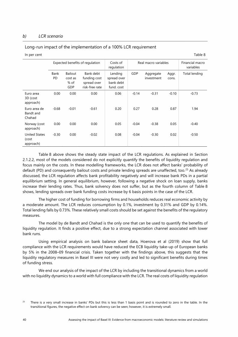
40 Assessing the impact of Basel III: Evidence from macroeconomic models: literature review and simulations
b) LCR scenario
Long-run impact of the implementation of a 100% LCR requirement In per cent Table 8
Expected benefits of regulation Costs of regulation
Real macro variables Financial macro variables
Bank PD
Bailout cost as % of GDP
Bank debt funding cost spread over risk-free rate
Lending spread over bank debt fund. cost
GDP Aggregate investment
Aggr. cons.
Total lending
Euro area 3D (cost approach)
0.00 0.00 0.00 0.06 -0.14 -0.31 -0.10 -0.73
Euro area de Bandt and Chahad
-0.68 -0.01 -0.61 0.20 0.27 0.28 0.87 1.94
Norway (cost approach)
0.00 0.00 0.00 0.05 -0.04 -0.38 0.05 -0.40
United States (cost approach)
-0.30 0.00 -0.02 0.08 -0.04 -0.30 0.02 -0.50
Table 8 above shows the steady state impact of the LCR regulations. As explained in Section 2.1.2.2, most of the models considered do not explicitly quantify the benefits of liquidity regulation and focus mainly on the costs. In these modelling frameworks, the LCR does not affect banks’ probability of default (PD) and consequently bailout costs and private lending spreads are unaffected, too.25 As already discussed, the LCR regulation affects bank profitability negatively and will increase bank PDs in a partial equilibrium setting. In general equilibrium, however, following a negative shock on loan supply, banks increase their lending rates. Thus, bank solvency does not suffer, but as the fourth column of Table 8 shows, lending spreads over bank funding costs increase by 6 basis points in the case of the LCR.
The higher cost of funding for borrowing firms and households reduces real economic activity by a moderate amount. The LCR reduces consumption by 0.1%, investment by 0.31% and GDP by 0.14%. Total lending falls by 0.73%. These relatively small costs should be set against the benefits of the regulatory measures.
The model by de Bandt and Chahad is the only one that can be used to quantify the benefits of liquidity regulation. It finds a positive effect, due to a strong expectation channel associated with lower bank runs.
Using empirical analysis on bank balance sheet data, Hoerova et al (2019) show that full compliance with the LCR requirements would have reduced the ECB liquidity take-up of European banks by 5% in the 2008–09 financial crisis. Taken together with the findings above, this suggests that the liquidity regulatory measures in Basel III were not very costly and led to significant benefits during times of funding stress.
We end our analysis of the impact of the LCR by including the transitional dynamics from a world with no liquidity dynamics to a world with full compliance with the LCR. The real costs of liquidity regulation
25 There is a very small increase in banks’ PDs but this is less than 1 basis point and is rounded to zero in the table. In the
transitional figures, the negative effect on bank solvency can be seen; however, it is extremely small.

Assessing the impact of Basel III: Evidence from macroeconomic models: literature review and simulations 41
are not very large mainly because the cost to banks of holding liquid assets or of funding with long-term (rather than short-term) debt is not very high.
The cost of the LCR would rise significantly if three things happen:
(a) The yield of HQLA falls further relative to that of deposits, increasing the cost to banks of holding HQLA.
(b) The capital risk weight on HQLA increases meaning that HQLA holdings will consume bank capital.
(c) Banks are constrained by the leverage ratio, so that they need to substitute HQLA to higher yielding assets.
2.2.2 On business cycle fluctuations
All models exhibit a decrease in volatility when moving to Basel III (even without introducing the CCyB), but the impact is not very sizeable (see Annex 3 for details).
2.2.3 On the transition from Basel II to Basel III
a) For the solvency scenario
Note that most models highlight the role of monetary policy reaction in accompanying the reforms, by reducing the policy rate at the start of the implementation period. We illustrate the monetary policy response in Graph 1 by the case of an increase of the capital ratio by 2.5 percentage points for the euro area with the 3D model.
Transition from 14% capital ratio to 16.5% in the euro area with 3D model Graph 1
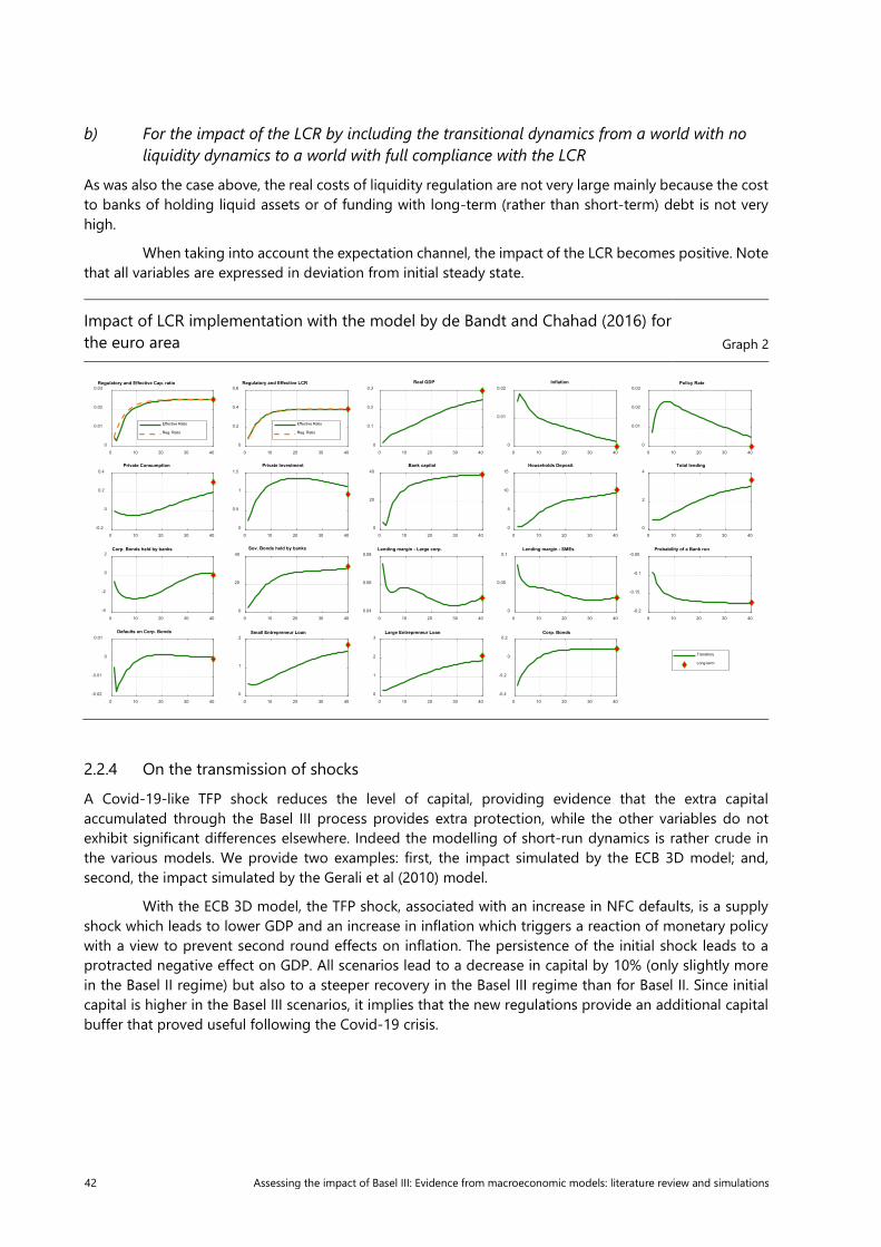
42 Assessing the impact of Basel III: Evidence from macroeconomic models: literature review and simulations
b) For the impact of the LCR by including the transitional dynamics from a world with no liquidity dynamics to a world with full compliance with the LCR
As was also the case above, the real costs of liquidity regulation are not very large mainly because the cost to banks of holding liquid assets or of funding with long-term (rather than short-term) debt is not very high.
When taking into account the expectation channel, the impact of the LCR becomes positive. Note that all variables are expressed in deviation from initial steady state.
Impact of LCR implementation with the model by de Bandt and Chahad (2016) for the euro area Graph 2
2.2.4 On the transmission of shocks
A Covid-19-like TFP shock reduces the level of capital, providing evidence that the extra capital accumulated through the Basel III process provides extra protection, while the other variables do not exhibit significant differences elsewhere. Indeed the modelling of short-run dynamics is rather crude in the various models. We provide two examples: first, the impact simulated by the ECB 3D model; and, second, the impact simulated by the Gerali et al (2010) model.
With the ECB 3D model, the TFP shock, associated with an increase in NFC defaults, is a supply shock which leads to lower GDP and an increase in inflation which triggers a reaction of monetary policy with a view to prevent second round effects on inflation. The persistence of the initial shock leads to a protracted negative effect on GDP. All scenarios lead to a decrease in capital by 10% (only slightly more in the Basel II regime) but also to a steeper recovery in the Basel III regime than for Basel II. Since initial capital is higher in the Basel III scenarios, it implies that the new regulations provide an additional capital buffer that proved useful following the Covid-19 crisis.
0 10 20 30 40
0
0.01
0.02
0.03Regulatory and Effective Cap. ratio
Effective Ratio
Reg. Ratio
0 10 20 30 40
0
0.2
0.4
0.6Regulatory and Effective LCR
Effective Ratio
Reg. Ratio
0 10 20 30 40
0
0.1
0.2
0.3Real GDP
0 10 20 30 40
0
0.01
0.02Inflation
0 10 20 30 40
0
0.01
0.02
0.03Policy Rate
0 10 20 30 40
-0.2
0
0.2
0.4Private Consumption
0 10 20 30 40
0
0.5
1
1.5Private Investment
0 10 20 30 40
0
20
40Bank capital
0 10 20 30 40
0
5
10
15Households Deposit
0 10 20 30 40
0
2
4Total lending
0 10 20 30 40
-4
-2
0
2Corp. Bonds held by banks
0 10 20 30 40
0
20
40Sov. Bonds held by banks
0 10 20 30 40
0.04
0.06
0.08Lending margin - Large corp.
0 10 20 30 40
0
0.05
0.1Lending margin - SMEs
0 10 20 30 40
-0.2
-0.15
-0.1
-0.05Probability of a Bank run
0 10 20 30 40
-0.02
-0.01
0
0.01Defaults on Corp. Bonds
0 10 20 30 40
0
1
2Small Entrepreneur Loan
0 10 20 30 40
0
1
2
3Large Entrepreneur Loan
0 10 20 30 40
-0.4
-0.2
0
0.2Corp. Bonds
Transitory
Long-term

Assessing the impact of Basel III: Evidence from macroeconomic models: literature review and simulations 43
Impulse response function of an adverse shock on TFP and NFC default rate (euro area with 3D model) Transitions following a -25% TFP shock and NFC default rate up to 15% Graph 3
Similar results are found with a version of the Gerali et al (2010) for the euro area with a TFP shock (-14.4%) complemented by an additional shock to private investment (-27.6%). Such a calibration of shocks is designed to replicate a GDP drop by 8% one year after the shock arrives. TFP and investment shocks have opposite effects on inflation: the investment shock reduces the positive pressure on inflation caused by the TFP shock. Overall, this will trigger a smaller increase in the policy rate than under the TFP shock presented above with the 3D model. The collateral channel prevails, and lending falls. However, the benefits of Basel III are more visible for housing loans than for NFC loans. Indeed the reduction in housing loans is more significant in Basel II than in the two Basel III scenarios, showing that the collateral channel is somewhat less strong when banks are better capitalised. In addition, banks exhibit a cyclical reaction: in the short run, the increase in lending rates positively affects profits and capital.

44 Assessing the impact of Basel III: Evidence from macroeconomic models: literature review and simulations
Impulse response function of an adverse shock on TFP and investment (euro area with Gerali et al (2010) framework) Impulse responses to TFP and investment shocks under different levels of CET1 ratios Graph 4
2.3 Conclusions of simulation exercises and suggestions for next steps
Several conclusions may be drawn from this exercise.
• The calibration/measurement of the bank default probability (or financial crisis probability) and its evolution plays a crucial role in the assessment.
• The expectation channel plays an important role, conditioning the final impact of the reforms: if economic agents anticipate that the reforms will effectively reduce the probability of bank failure or the probability of a run, this triggers, beyond the initial supply shock, a positive demand effect on GDP.
• The modelling of short-run dynamics is still incomplete, while long-run impacts are satisfactory.
Regarding the main questions, the macro models are in agreement with initial LEI (BCBS (2010)) qualitative conclusions.
Regarding future research, one should investigate several of the issues that have not been addressed in the simulations considered here. These issues have been studied, although only very recently, in the stylised financial models reviewed in Section 1.2:
• The role of unconventional monetary policy.
• The role of the shadow banking sector.
• The role of systemic risk.
• A more comprehensive analysis of large shocks, Covid-19-like.

Assessing the impact of Basel III: Evidence from macroeconomic models: literature review and simulations 45
• Further analysis of liquidity and interactions between policies.
• Regarding macroeconomic shocks and variables: a more detailed analysis of the impact on inflation and welfare.
3. General conclusion
1. The literature review has highlighted the variety of models that have been produced since the GFC. The conclusion is that most of the models show that Basel III leads to an increase in GDP, while some models show negative effects. The increase in GDP comes through an initial supply shock, which may translate into a demand shock as economic agents expect a decrease in banking instability.
2. However, the models only offer a partial assessment of the macroeconomic impact of the new regulatory environment. In particular, when assessing the effects of banking regulations, it is crucial to distinguish models that assess both costs and benefits (eg the 3D model and NEMO) from models that are mostly used for assessing costs (Gerali et al (2010)).
The following limitations have been identified:
• The models are still quite stylised with only one capital variable, total capital.
• In addition, funding liquidity has only been incorporated in a basic way.
• Liquidity regulation is not fully integrated in most models.
One conclusion may be that there is no perfect model. Quantitative DSGE models basically focus on capital requirements. Empirical models lack micro-foundations, which is problematic for policy analysis. Complicated issues, such as interactions between multiple regulations, still depend on qualitative models.
3. There is scope for further research regarding the role of shadow banking, the interaction between unconventional monetary policy and financial stability policy.
4. Possible next steps: Taking stock of the literature review and the recent advances in modelling, the next stage could be to build a quantitative model that explicitly considers the most important costs and benefits of capital and liquidity regulations. These costs and benefits have already been identified (such as reduced crisis probability and crisis severity against higher spreads and lower output in normal times). Both capital and liquidity regulations should be incorporated into the model. The best (and the most time-efficient) strategy going forward can be to take a workhorse model with the most important ingredients included among the papers reviewed here and incorporate some key features if necessary.

46 Assessing the impact of Basel III: Evidence from macroeconomic models: literature review and simulations
References
Adrian, T and N Boyarchenko (2018): “Liquidity policies and systemic risk”, Journal of Financial Intermediation, vol 35B, pp 45–16.
Adrian, T, N Boyarchenko and D Giannone (2019): “Vulnerable growth”, American Economic Review, vol 109, pp 1263–89.
Angeloni, I and E Faia (2013): “Capital regulation and monetary policy with fragile banks”, Journal of Monetary Economics, vol 60, pp 311–324.
Arbatli-Saxegaard, E, K R Gerdrup and R M Johansen (2020): “Financial imbalances and medium-term macroeconomic tail risks in Norway”, Norges Bank Staff memo, no 5/2020.
Aruoba, B, P Cuba-Borda and F Schorfheide (2018): “Macroeconomic dynamics near the ZLB: A tale of two countries”, Review of Economic Studies, vol 85, pp 87-118.
Barrell, R, E P Davis, T Fic, D Holland, S Kirby and I Liadze (2009): “Optimal regulation of bank capital and liquidity: how to calibrate new international standards”, FSA Occasional Paper, no 38.
Basel Committee on Banking Supervision (2010): An assessment of the long-term economic impact of stronger capital and liquidity requirements, www.bis.org/publ/bcbs173.htm.
——— (2016): “Literature review on integration of regulatory capital and liquidity instruments”, Basel Committee on Banking Supervision Working Papers, no 30, March, www.bis.org/bcbs/publ/wp30.htm.
——— (2019): “The costs and benefits of bank capital: a review of the literature”, Basel Committee on Banking Supervision Working Papers, no 37, June, www.bis.org/bcbs/publ/wp37.htm.
Begenau, J (2020): “Capital requirements, risk choice, and liquidity provision in a business-cycle model”, Journal of Financial Economics, vol 136 (2), pp 355-378.
Benigno, G, H Chen, C Otrok, A Rebucci and E R Young (2013) “Financial crises and macro-prudential policies”, Journal of International Economics, vol 89, no 2, pp 453–470.
Bennani, T, C Couaillier, A Devulder, S Gabrieli, J Idier, P Lopez, T Piquard and V Scalone (2017): “An analytical framework to calibrate macroprudential policy”, Banque de France, Working Paper no 648.
Bernanke, B (2005): “The global saving glut and the US current account deficit”, Speech, Board of Governors of the Federal Reserve System.
——— (2018): “The real effects of the financial crisis”, in Brooking Papers on Economic Activity, Conference Drafts, September, vol 13.
Bernanke, B, M Gertler and S Gilchrist (1996): “The financial accelerator in a quantitative business cycle framework”, Review of Economics and Statistics, vol 78, pp 1–15.
——— (1999): “The financial accelerator in a quantitative business cycle framework”, Handbook of Macroeconomics, vol 1, pp 1341–1393.
Bianchi, J and E G Mendoza (2018): “Optimal time-consistent macroprudential policy”, Journal of Political Economics, vol 126, no 2, pp 588–634.
Birn, M, O de Bandt, S Firestone, M Gutiérrez Girault, D Hancock, T Krogh, H Mio, D P Morgan, A Palvia, V Scalone, M Straughan and A Uluc (2020): "The costs and benefits of bank capital – a review of the literature", Journal of Risk and Financial Management, MDPI, Open Access Journal, vol 13, no 4, April, pp 1–25.
Boissay, F and F Collard (2016): “Macroeconomics of bank capital and liquidity regulations”, BIS Working Paper, no 596, www.bis.org/publ/work596.htm.

Assessing the impact of Basel III: Evidence from macroeconomic models: literature review and simulations 47
Boissay, F, F Collard and F Smets (2016): “Booms and banking crises”, Journal of Political Economy, vol 124, no 2, pp 489–538.
Brunnermeier, M and Y Sannikov (2014): “A macroeconomic model with a financial sector”, American Economic Review, vol 104, no 2, pp 379–421.
Calvo, G (1983): “Staggered prices in a utility-maximizing framework”, Journal of Monetary Economics, vol 12, no 3, pp 383–398.
——— (1988): "Servicing the public debt: the role of expectations”, American Economic Review, vol 78, pp 647–661.
Central Bank of Norway (2019): Financial Stability Report: vulnerabilities and risks, www.norges-bank.no/en/news-events/news-publications/Reports/Financial-Stability-report/financial-stability-2019/.
Clerc, L, A Derviz, C Mendicino, S Moyen, K Nikolov, L Stracca, J Suarez and A P Vardoulakis (2015): “Capital regulation in a macroeconomic model with three layers of default”, International Journal of Central Banking, vol 11, no 3, pp 9–63.
Coimbra, N and H Rey (2020): “Financial cycles with heterogeneous intermediaries”, NBER Working Papers, no 23245.
Cole, H and T Kehoe (2000): “Self-fulfilling debt crises”, Review of Economic Studies, vol 67, pp 91–161.
Conti, A M, A Nobili and F M Signoretti (2018): “Bank capital constraints, lending supply and economic activity”, Banca d’Italia Working Paper, no 1199.
Covas, F and J C Driscoll (2014): “Bank liquidity and capital regulation in general equilibrium”, Finance and Economics Discussion Series, Federal Reserve Board.
Curdia, V and M Woodford (2010): "Conventional and unconventional monetary policy", Review, Federal Reserve Bank of St. Louis, vol 92, May, pp 229–264.
Davila, E and A Korinek (2018): “Pecuniary externalities in economies with financial frictions”, Review of Economic Studies, vol 85, pp 352–395.
de Bandt, O and M Chahad (2016): “A DSGE model to assess the post crisis regulation of universal banks”, Banque de France, Working Paper 602, publications.banque-france.fr/sites/default/files/medias/documents/working-paper_602_2016.pdf.
de Bandt, O, S Lecarpentier and C Pouvelle (2021): “Determinants of banks’ liquidity: A French perspective on interactions between market and regulatory requirements”, forthcoming, Journal of Banking and Finance, doi.org/10.1016/j.jbankfin.2020.106032.
De Nicolò, G, A Gamba and M Lucchetta (2014): “Microprudential regulation in a dynamic model of banking”, Review of Financial Studies, vol 27, no 7, pp 2097–138.
de-Ramon, S and M Straughan (2017): "The economic cost of capital: a VECM approach for estimating and testing the banking sector's response to changes in capital ratios", Bank of England Staff Working Paper, no 663.
Dewatripont, M and J Tirole (2018): "Liquidity regulation, bail-ins and bailouts", manuscript, www.tse-fr.eu/sites/default/files/TSE/documents/doc/by/tirole/prudential_treatment_of_liquidity_080618.pdf.
Diamond, D W and P H Dybvig (1983): “Bank runs, deposit insurance, and liquidity”, Journal of political economy, vol 91, no 3, pp 401–419.
Durdu, B and M Zhong (2019): “Understanding bank and nonbank credit cycles: a structural exploration”, Finance and Economics Discussion Series, no 2019-031, Board of Governors of the Federal System, www.federalreserve.gov/econres/feds/understanding-bank-and-nonbank-credit-cycles-a-structural-exploration.htm.

48 Assessing the impact of Basel III: Evidence from macroeconomic models: literature review and simulations
Elenev, V, T Landvoigt and S Van Nieuwerburgh (2020): “A macroeconomic model with financially constrained producers and intermediaries”, forthcoming, Econometrica.
Gambacorta, L (2011): “Do bank capital and liquidity affect real economic activity in the long run? A VECM analysis for the US”, Economic Notes, vol 40, no 3, pp 75–91.
Gambacorta, L and H S Shin (2018): “Why bank capital matters for monetary policy”, Journal of Financial Intermediation, vol 35, part B, pp 17-29.
Gelain, P, K J Lansing and G J Natvik (2018): “Explaining the boom-bust cycle in the U.S. housing market: a reverse-engineering approach”, Journal of Money, Credit and Banking, vol 50, pp 1751–83.
Gerali, A, S Neri, L Sessa and F M Signoretti (2010): “Credit and banking in a DSGE model of the euro area”, Journal of Money, Credit and Banking, vol 42, pp 107–41.
Gerdrup, K R, F Hansen, T Krogh and J Maih (2017): “Leaning against the wind when credit bites back”, International Journal of Central Banking, vol 13, no 3, pp 287–320.
Gertler, M and P Karadi (2011): “A model of unconventional monetary policy”, Journal of Monetary Economics, vol 58, no 1, pp 17–34.
Gertler, M and N Kiyotaki (2015): “Banking, liquidity and bank runs in an infinite horizon economy”, American Economic Review, vol 105, pp 2011–43.
Gertler M, N Kiyotaki and A Prestipino (2019): “A macroeconomic model with financial panics”, Review of Economic Studies, vol 87, no 1, pp 240–88.
He, Z and A Krishnamurthy (2019): “A macroeconomic framework for quantifying systemic risk”, American Economic Journal, vol 11, pp 1–37.
Hoerova, M, C Mendicino, K Nikolov, G Schepens and S Van den Heuvel (2018): "Benefits and costs of liquidity regulation", ECB Working Paper, no 2169, ideas.repec.org/p/ecb/ecbwps/20182169.html.
Holden, T D, P Levine and J M Swarbrick (2019): “Credit crunches from occasionally binding bank borrowing constraints”, Journal of Money, Credit and Banking, vol 52, no 2–3, pp 549–82.
Holmström, B and J Tirole (1997): “Financial intermediation, loanable funds, and the real sector”, Quarterly Journal of Economics, vol 112, pp 663–91.
Iacoviello, M (2005): "House prices, borrowing constraints, and monetary policy in the business cycle", American Economic Review, vol 95, no 3, pp 739–64.
Ikeda, D (2018): "Bank runs, prudential tools and social welfare in a global game general equilibrium model", Bank of England Working Paper, no 732, www.bankofengland.co.uk/-/media/boe/files/working-paper/2018/bank-runs-prudential-tools-and-social-welfare-in-a-global-game-general-equilibrium-model.pdf.
Jeanne, O and A Korinek (2019): “Managing credit booms and busts: A Pigovian taxation approach”, Journal of Monetary Economics, vol 107, pp 2–17.
——— (2020): “Macroprudential regulation versus mopping up after the crash”, Review of Economic Studies, vol 87, no 3, pp 1470–97.
Jondeau E and J-G Sahuc (2018): “A general equilibrium appraisal of capital shortfall”, Banque de France Working Paper 668, papers.ssrn.com/sol3/papers.cfm?abstract_id=3126905.
Jorda, O, B Richter, M Schularick and A Taylor (2017): “Bank capital redux: solvency, liquidity, and crisis”, NBER Working Paper, no 23287, March.
Kashyap, A K, D P Tsomocos and A P Vardoulakis (2020): "Optimal bank regulation in the presence of credit and run-risk", NBER Working Papers, no 26689.

Assessing the impact of Basel III: Evidence from macroeconomic models: literature review and simulations 49
Kiyotaki, N and J Moore (1997): “Credit cycles”, Journal of Political Economy, vol 105, no 2, pp 211–48.
Kockerols, T, E M Kravik and Y Mimir (2021): Leaning against the wind in the face of persistent financial cycles and occasional crises, Norges Bank, mimeo.
Korinek, A and E G Mendoza (2014): “From sudden stops to Fisherian deflation: quantitative theory and policy”, Annual Economic Review, vol 6, pp 299–332.
Korinek, A and A Simsek (2016): ”Liquidity trap and excessive leverage”, American Economic Review, vol 106, no 3, pp 699–738.
Kravik, E M and Y Mimir (2019): “Navigating with NEMO”, Norges Bank Staff Memo, no 5/2019.
Macroeconomic Assessment Group (2010): “Assessing the macroeconomic impact of the transition to stronger capital and liquidity requirements”, Bank for International Settlements, Basel.
Martinez-Miera, D and R Repullo (2017): “Search for yield”, Econometrica, vol 85, no 2, pp 351–78.
——— (2019): “Markets, banks and shadow banks”, ECB Working Paper, www.ecb.europa.eu/pub/conferences/shared/pdf/20180517_3rd_mp_policy_research/2018-05-17_Paper_Repullo_Markets_banks_and_shadow_banks_paper.pdf.
Martinez-Miera, D and J Suarez (2014): Banks’ endogenous systemic risk taking, September 2014, www.cemfi.es/~suarez/mmiera-suarez2014.pdf.
Meh, C A and K Moran (2010): “The role of bank capital in the propagation of shocks”, Journal of Economic Dynamics and Control, vol 34, no 3, pp 555–76.
Mendicino, C, K Nikolov, J Suarez and D Supera (2018): “Optimal dynamic capital requirements”, Journal of Money, Credit and Banking, vol 50, no 6, pp 1271–97.
——— (2020): “Bank capital in the short and in the long run”, Journal of Monetary Economics (forthcoming), ideas.repec.org/p/ecb/ecbwps/20192286.html.
Mendoza, E G (2010): “Sudden stops, financial crises, and leverage”, American Economic Review, vol 100, no 5, pp 1941–66.
Mendoza E G and K A Smith (2006): “Quantitative implications of a debt deflation theory of sudden stops and asset prices”, Journal of International Economics, vol 70, no 1, pp 82–114.
Mikkelson, J and J Pedersen (2017): “A cost-benefit analysis of capital requirements for the Danish economy”, Danmarks Nationalbank Working Paper, no 123.
Miller, S and R Sowerbutts (2018): “Bank liquidity and the cost of debt”, Bank of England Staff Working Paper, no 707, www.bankofengland.co.uk/working-paper/2018/bank-liquidity-and-the-cost-of-debt.
Mordel, A (2018): "Prudential liquidity regulation in banking – a literature review", Bank of Canada Staff Discussion Paper, no 2018-8, www.bankofcanada.ca/2018/07/staff-discussion-paper-2018-8.
Pedersen, J (2016): “An estimated DSGE model for Denmark with housing, banking and financial frictions”, Danmarks Nationalbank Working Paper, no 108.
Schroth, J (2021): “Macroprudential policy with capital buffers”, Journal of Monetary Economics, forthcoming, doi.org/10.1016/j.jmoneco.2020.12.003.
Schularick, M and A M Taylor (2012): “Credit booms gone bust: Monetary policy, leverage cycles, and financial crises, 1870-2008”, American Economic Review, vol 102, no 2, pp 1029–61.
Smets, F and R Wouters (2003): “An estimated Dynamic Stochastic General Equilibrium Model of the euro area”, Journal of the European Economic Association, vol 1, no 5, pp 1123–75.
Swarbrick, J (2019): "Lending standards, productivity and credit crunches", Bank of Canada Staff Working Papers, no 2019-25, www.bankofcanada.ca/wp-content/uploads/2019/07/swp2019-25.pdf.

50 Assessing the impact of Basel III: Evidence from macroeconomic models: literature review and simulations
Van den Heuvel, S (2019): "The welfare effects of bank liquidity and capital requirements", 2019 Meeting Papers 325, Society for Economic Dynamics, ideas.repec.org/p/red/sed019/325.html.
Walther, A (2016): “Jointly optimal regulation of bank capital and liquidity”, Journal of Money, Credit and Banking, vol 48, no 2–3, pp 415–48.

Assessing the impact of Basel III: Evidence from macroeconomic models: literature review and simulations 51
Annex 1: Measurement issues associated with the scenarios
Two issues are discussed in this Annex:
• the measurement of default probability which has a significant impact on the assessment of costs and benefits of regulation;
• the calibration of the overall risk environment.
1. Discussion about the measurement of bank default probability
In the 3D model, the ex ante probability of bank default plays a prominent role in determining the costs and benefits of capital requirement changes and its calibration is therefore very important. We discuss here a few measurement challenges.
One way to measure the probability of bank failure is by looking at the frequency of actual bank defaults over the past. While easy to implement, this has drawbacks for a number of reasons. During stable periods, very few banks fail. In addition, even during crisis times, not all insolvent banks fail due to extensive government assistance to the financial sector. If such government assistance is itself costly (for example due to tax costs or ex ante moral hazard), the need for such ex post state intervention is something capital regulation should be seeking to avoid. Thus, low numbers of actual bank defaults is not something which necessarily signals that banks are safe.
A conceptually more accurate measure of ex ante bank risk is the Expected Default Frequency (EDF), a measure popularised by Moody’s KMV. This is a measure which uses a Black-Scholes option pricing framework and computes the probability that a bank will become insolvent based on its leverage (as well as other balance sheet factors) and the volatility of its share price. More volatility implies a greater likelihood of insolvency according to the EDF measure. This measure is less distorted by potential state interventions than counting actual defaults and is therefore a better measure of how risky a bank is.
The EDF measure is not without problems, however. It captures bank risk accurately only if the stock market always values companies in a fully efficient manner. There exists considerable research showing that stock prices are much more volatile than the NPV of future dividend streams. If the volatility of share prices is greater than the volatility of the value of bank assets, then the EDF measure overstates the true risk of bank failure.
In the end, there does not exist a perfect measure. We assume a probability of bank default of 0.5% per annum, which lies between the two different types of measures and represents a significant, but not excessive, risk of bank failure. To examine the sensitivity of our findings with respect to this measure, we have repeated the steady state analysis with bank failure measures of 0.2% and 0.8% per annum. These results show that net benefits of Basel III are much larger for the higher risks of bank failure.
2. Discussion about the calibration of bank risk and the conduct of the exercise
Conceptually it is not easy to develop a method to evaluate the effects of a policy measure such as Basel III, which was introduced in response to a financial crisis. There is no exogenous variation in capital requirements we can rely on in order to trace the impact of higher bank capital on the real economy and

52 Assessing the impact of Basel III: Evidence from macroeconomic models: literature review and simulations
the financial system. Since the financial crisis, we observe a significant increase in banks’ capital ratios reflecting both tighter regulatory minimum standards as well as greater voluntary capital buffers above the minimum. At the same time, we observe bank riskiness as measured by average asset-weighted EDF measures, which remain stubbornly above pre-crisis levels. This shows how public policy (Basel III) as well as banks’ own prudential standards (voluntary buffers) have reacted to a big increase in underlying risk facing financial institutions. Such changes in risk perceptions may have come from a combination of legacy asset problems as well as structural challenges to profitability and business models such as competition from fintech start-ups, flat yield curves world-wide and the realisation that sovereign debt holdings are not risk-free.
To evaluate the impact of moving from Basel II to Basel III, we cannot simply take a pre-crisis calibration and increase capital requirements because so much has already changed since 2007. Instead, we conduct Basel II counterfactuals by asking the question: “What would the world look like today if we did not have Basel III?” We calibrate the model to match the current risk of bank failure and we lower bank capital ratios by the amount we judge to be due to the move from Basel II to Basel III. In conducting this step in the analysis, we face two key challenges.
One is how to treat the increase in banks’ voluntary buffers. Is this increase driven by more stringent regulation and supervision in the Basel III world or is it a voluntary reaction by banks to a riskier environment? Our simple approach is to treat banks’ voluntary buffers as given and to assume that capital ratios would have been lower in a Basel II counterfactual by the difference between Basel III and Basel II minimum capital ratios. This understates the benefits from tighter regulation since it is likely that at least some of the additional voluntary buffer build-up was driven by the increased threat of regulatory interventions in undercapitalised fail stress tests for example.
The second challenge is how to map from the rich set of new regulatory measures in Basel III to the stylised nature of the models, which fail to distinguish between Tier 1 and Tier 2 capital for example. One simple approach would be to assume that only total (Tier 1 + Tier 2) capital matters. Under such an approach, Basel III increased banks’ capital ratios by 2.5 percentage points once the capital conservation buffer is fully loaded.
This would, however, ignore the beneficial changes in the composition of capital, which increased the minimum Tier 1 ratio from 4% to 6% (and the CET1 ratio from 2% to 4.5%). To capture the Basel III benefits coming from higher quality as well as quantity of bank capital, we consider an alternative (much more adverse) Basel II counterfactual in which bank capital ratios are 5 percentage points lower than their current levels. The estimated benefits of Basel III will be much larger under this approach.
Assessing the impact of Basel III: Evidence from macroeconomic models: literature review and simulations 53
Annex 2: Definition of the scenarios
Baseline scenarios implemented in Part 2 of the report focus on capital requirements, but also investigate liquidity requirements.
1. Capital requirements increase by 2.5 percentage points or 5 percentage points. The scenarios assess the real and financial stability effects of moving from Basel II (eg 8% total capital ratio (TCR) in the euro area) to Basel III, either (i) 10.5% TCR (including the capital conservation buffer) or (ii) 13% TCR (including the capital conservation buffer and accounting for the higher quality of capital requirements); in both cases taking into account voluntary capital buffers.
a. The models are calibrated to the recent past (with eg in the euro area a 10.5% minimum TCR and voluntary buffers on top; or 13% TCR and voluntary buffer on top).
b. A steady state counterfactual (variant scenario) is computed with an 8% TCR plus the same voluntary capital buffer as computed under (a) above.
i. The probability of bank failure is computed under the two steady states.
ii. As well as the differences in the levels of output, business and housing investment, business and household lending and consumption.
iii. The existence of significant differences in the impact on different economic agents (borrowers vs savers) in terms of housing ownership, consumption and employment are also assessed. The channels by which capital requirements affect the economy and welfare are explained.
c. The transition between the two steady states is computed assuming a partial adjustment of the TCR to its new higher level over five years:26
i. Assessment of the transitional costs in terms of output, investment (business and housing), lending (business and housing).
ii. As well as the differences between borrowers and savers.
d. In order to assess the impact of the reforms on the cyclical behaviour of the economy, the first and second moments of the distribution of key macro variables (output, investment, lending) are computed.
Particular attention will be put in b–d on possible non-linearities by comparing (i) 10.5% TCR and (ii) 13% TCR
26 The process for implementing the increase in the TCR is of the following form: TCR(t) = rho_TCR*TCR(t-1) + (1-
rho_TCR)*TCR(Basel III). The simulation starts with an initial condition equal to TCR(Basel II) (8% + the voluntary capital buffers in place right now). TCR(Basel III) is the new Basel III minimum (either 10.5% or 13%) plus the voluntary buffers in place right now. We propose a value of rho_TCR = 0.8 to ensure that TCR(t) is close to TCR(Basel III) after 20 quarters.

54 Assessing the impact of Basel III: Evidence from macroeconomic models: literature review and simulations
2. The real economy costs of the LCR.
a. Either the LCR is introduced as an additional constraint on banks with effects on the probability of a bank run (implementing an increase of the ratio by 40 percentage points corresponding to an increase from 60% to 100%); or
b. Only the impact on bank profits are assessed (“cost approach”). In that case, the simulations follow the approach of Hoerova et al (2018).
The LCR is introduced as a requirement for banks to hold HQLA in proportion to short-term demandable debt/deposits. This has two effects as explained in the appendix of Hoerova et al (2018):
i. If the risk weight on the HQLA is zero, there will still be an impact as long as the (interest and non-interest) cost of issuing bank deposits is higher than the return on HQLA. The LCR will then reduce bank profits (all things equal).27 In general equilibrium, this will require higher lending rates with a contractionary impact on lending and real activity. The higher costs from the LCR and the higher lending rates offset each other so the solvency of the bank is broadly unaffected.
ii. If the HQLA carry a positive risk weight (or if banks face a binding leverage ratio), the HQLA will consume capital and private sector lending will fall further compared to the previous case. If the HQLA are riskless, the probability of failure of the bank will decline because the higher LCR will act as an increase in the capital requirement.
3. Numerical exercise:
i. LCR on a standalone basis: The scenarios investigate whether the LCR crowds out lending or reduce output, consumption and investment. With a zero risk weight experiment, it was found in Hoerova et al (2018) that the real impact (GDP, lending, etc) was negative but pretty small as the LCR is not so costly for banks.
ii. The joint implementation of capital regulation (10.5% TCR, or increase by 2.5 percentage points) and LCR is also assessed.
27 One short-cut for introducing the LCR is to reduce profits from the opportunity cost to hold HQLA.

Assessing the impact of Basel III: Evidence from macroeconomic models: literature review and simulations 55
Annex 3: Detailed analysis of the country results
1. Euro area by the European Central Bank28
After a more complete description of the 3D model than in Part 1, the results of the scenarios are presented in greater detail. As described in Section 1.1.1, a key mechanism is the impact of higher capital requirements on a lower level of bank failures, hence triggering a lower cost of uninsured debt, and financial intermediation. This has a positive effect on GDP when the economy starts from a high level of bank failures.
1.1 Model description
The model we use is a significantly modified version of the Clerc et al (2015) framework with three layers of default. The model agents are a representative worker-saver household, a representative worker-borrower household, entrepreneurs (who provide equity funding to firms) and bankers (who provide equity funding to banks), one period-lived firms and banks. Defaults occur for firms, mortgage borrowers and banks.
The 3D model is modified in several key respects. We have added the following features:
• Calvo (1983) nominal rigidities and a Taylor rule to implement monetary policy.
• A non-bank sector (direct production by the household subject to a cost).
• Banks can issue equity/reduce dividends in order to speed up bank capital accumulation.
The calibration of the model is presented in Annex 4.
1.2 Key mechanisms governing the relationship between capital requirements and economic activity and welfare
1.2.1 Impact of capital requirements on economic activity
Banks in the 3D model are competitive. They provide loans to firms and households at marginal cost. The weighted average cost of capital (WACC) for banks is the weighted average of the cost of equity and the cost of bank debt. When WACC rises, banks increase lending rates and the economy suffers. Capital requirements affect WACC in two offsetting ways:
• Since equity is more expensive than debt, raising capital requirements increases banks’ WACC and this reduces economic activity.
• In our euro area calibration, 45% of debt is uninsured and pays a risk premium over the risk free rate in order to compensate debt holders for the risk of default. Higher capital requirements make banks safer and reduce the default risk premium, bringing down the cost of bank debt. This lowers WACC, other things equal.
• When the probability of bank default is high, the debt cost channel dominates and higher capital requirements reduce banks’ WACC and lending and economic activity increase. When the
28 By Kalin Nikolov (European Central Bank).

56 Assessing the impact of Basel III: Evidence from macroeconomic models: literature review and simulations
probability of bank default is low, the liability composition channel dominates and higher capital requirements reduce lending and economic activity.
1.2.2 Impact of capital requirements on welfare
Capital requirements affect welfare through three main channels:
• The level of wages: If capital requirements increase capital accumulation, wage income increases for all households, boosting consumption.
• Deadweight losses from default: Defaults destroy resources and reduce household wealth either through losses on uninsured bank debt (this affects only saver households) or through taxes that need to be levied in order to pay out on insured deposits (this affects all households because everyone is a tax payer). These public costs of debt are ignored by private borrowers, leading to excessive borrowing and investment. It is therefore possible for welfare to increase even if GDP falls as a result of higher capital requirements if investment had been excessive to begin with.
• The cost of mortgage debt: this affects only borrower households directly.
1.3 The impact of capital requirements on the level of macroeconomic variables
Table 9 shows how key variables change from Basel II to the Basel III baseline of 16.5% capital requirements (including a voluntary buffer above the minimum capital ratio). Crucially, the risks facing banks are held constant so the lower capital requirement under Basel II implies a much higher risk of bank failure. It is the reduction of this failure risk, which will bring the biggest welfare benefits in the 3D model.
Steady-state impact of a move from two different Basel II counterfactuals in the euro area (11.5% and 14% capital ratios) to the current (Basel III) level of the bank capital ratio (16.5%) using the 3D model by ECB Table 9
Capital ratio
Bank PD Bailout cost as % of GDP
Bank debt funding cost spread over
risk-free rate
Lending spread over bank debt
fund. cost
GDP Aggregate investment
Aggr. cons.
Total lending
+2.5 -1.72 -0.58 -0.13 0.12 0.18 -0.20 0.29 0.03
+5.0 -7.50 -2.55 -0.59 0.34 1.19 0.29 1.45 2.55
pp dev pp dev pp dev pp dev pp dev % dev % dev % dev % dev
A key benefit of increasing capital requirements is the reduction in the probability of bank failure, which declines by 1.7 percentage points. The Basel III baseline has a 0.5% bank PD whereas the Basel II counterfactual with 2.5 percentage points lower capital requirements has a 2.2% annual failure probability for banks. Fewer bank failures imply lower bank failure costs – both public and private.
The workout costs for failing banks (public costs) decline by 0.6% of annual GDP. These costs are ultimately born by all households because they are taxpayers who have to cover the cost of bailing out insured depositors. Fewer defaults and deadweight costs then leave more funds in the hands of households who increase consumption as a result.
The private costs are captured by the spread banks are forced to pay over the risk-free rate in order to attract debt funding. This spread declines by 0.13 percentage points on an annual basis. Some bank debt is uninsured and its interest rate decreases when banks are safer because debt holders no longer need to be compensated for the potential losses. Because banks are competitive, this cost reduction will be passed on to borrowers (ceteris paribus), stimulating economic activity.

Assessing the impact of Basel III: Evidence from macroeconomic models: literature review and simulations 57
Going in the opposite direction, a key cost of increasing capital requirements arises when the required rate of return on equity is higher than the cost of debt, which is assumed in the 3D model and in many other macro-financial models. This means that higher capital requirements should increase the spread of lending rates over deposit rates since banks with higher capital ratios need to achieve higher profitability in order to attract equity investors. Indeed, we see in the fourth column that the spread of lending interest rates over the bank’s debt funding declines by 0.12 percentage points.
The last four columns describe the overall macroeconomic implications of the policy. We see that the benefits from the policy outweigh the costs from the fact that GDP and consumption increase by, respectively, 0.2% and 0.3%. Aggregate investment declines by 0.2% and total lending is broadly unchanged.
Within total lending, banks tilt their lending towards loans with lower risk weights. This implies that household loans (risk weight of 0.5 in the model) actually increase a little while corporate lending (risk weight of one in the model) declines. This explains why investment declines. Consumption and overall GDP increase despite the fall in investment because the public cost of bank failures falls. When capital requirements are too low and some bank debt is uninsured, firms invest too much so that at the margin the total social cost of investment (including the public costs of bank failures) exceeds the total social benefit. When capital requirements reduce the risk of bank failure and reduce the excessive deadweight costs of bank default, this actually increases GDP net of default costs, improving welfare.
The second row of Table 9 examines a Basel II counterfactual bank capital ratio, which is 5 percentage points lower than the current Basel III one. This reflects the fact that Basel III improved not only the quantity but also the quality of bank capital by shifting the composition of total capital towards a more loss-absorbent form of bank liability – common equity. Yet again, because the risks facing bank solvency are assumed to be the same as in the Basel III baseline (16.5% bank capital ratio), the Basel II counterfactual scenario with 5 percentage points lower bank capital features much weaker banks with an extremely high probability of failure. As we will shortly see, this implies that the net benefits of introducing Basel III from this much more fragile Basel II counterfactual are even greater.
The bank default probability now declines by 7.5 percentage points from the implementation of Basel III because the bank annual default probability is 8% in the 11.5% Basel II counterfactual as compared to the 0.5% default probability in the 16.5% capital ratio baseline. The public cost of taxpayer bailouts falls by 2.5% of GDP while the private debt cost declines by almost 60 basis points. All of these benefits are very substantial and are driven by the very high probability of bank failure in the 11.5% capital requirement Basel II counterfactual.
Due to the larger increase in capital requirements considered in this case, the costs from the policy are also greater. This can be seen from the fact that the spread of bank lending rates over bank debt funding costs increases by 34 basis points.
Overall, the net benefits for the macroeconomy are very substantial. GDP rises by 1.2% driven by a 1.45% increase in consumption and a 0.3% increase in total investment. Total credit also increases by more than 2.5%. In this scenario, the reduction in the private cost of debt outweighs the increased costs due to a higher equity share. The private weighted average cost of capital for banks declines and lending and investment increase. Together with the decline in the public cost of bailing out failing banks, this ensures that consumption, GDP and welfare increase.
The benefits of increasing capital requirements are more than proportional in this more severe scenario. This is because the probability of bank default and its costs increase in a very non-linear manner the more undercapitalised banks are. In the Basel II counterfactual in which bank capital requirements are 5 percentage points lower than the Basel III baseline, banks are much more fragile and their probability of failure is 8% on an annualised basis (compared to only 2.2% in the Basel II counterfactual with capital requirements 2.5% below current levels).

58 Assessing the impact of Basel III: Evidence from macroeconomic models: literature review and simulations
1.4 Impact on the volatility of macroeconomic variables
The impact of capital requirements on second moments is shown in Table 10 below:
Second moments under Basel III (16.5% capital ratio) and under two different versions of Basel II Table 10
Macro variables Basel III Basel II
CR=16.5% CR=14% CR=11.5%
Real GDP 3.26 3.30 3.31
Total investment 8.40 8.61 8.83
Total lending 7.22 7.46 7.65
Bank failure probability 0.06 0.23 0.66
The table compares the annual standard deviations of variables under Basel III (the first column) and Basel II (columns 2 and 3). The volatility of GDP is slightly higher under Basel II driven by a substantial increase in the volatility of investment (in turn driven by more volatile lending). This is because investment is predominantly bank-funded in the model and its standard deviation is sensitive to the stability of the banking system. The volatility of consumption is actually slightly lower under Basel II compared to Basel III. This is due to the countercyclical response of monetary policy, which reacts more strongly to financial stability shocks when capital requirements are lower. Monetary policy does this to stabilise overall economic activity by boosting consumption in recessions to a greater extent. The volatility of the probability of bank failure is also considerably higher under Basel II reflecting the less solid capital position of banks. Under Basel III, the probability of bank failure is very stable, moving by a maximum of 0.1–0.15% (the standard deviation is 0.06%) in response to normal cyclical shocks.
1.5 Transitions from Basel II to Basel III
1.5.1 Capital requirements
We looked at how capital requirements change the first and second moments of key variables in the long term. We now consider the transition from Basel II to Basel III. The capital requirement is gradually increased either by 2.5 or by 5 percentage points over the space of five years, depending on the Basel II counterfactual scenario we consider. We already saw what the long-run impact of the policy would be in Table 9. We now see how the economy gets there.
When capital requirements increase, lending declines in the short term. Lending is restricted by bank equity and when capital requirements rise and raising new equity is costly, this initially forces banks to reduce the asset side of their balance sheet. Gradually, banks raise new equity or accumulate it through retained earnings.
The fall in lending hurts bank-dependent firms and borrower households who are forced to reduce expenditure. This depresses output, investment and consumption over the transition even if they rise in the long term. In the case when the Basel II capital ratio is 14% this actually leads to a small decline in real activity in the short term. In the case when the Basel II capital is 11.5%, banks have a very high risk of default (8% annualised bank PD). The increase in capital requirements then makes banks safer which is much more beneficial. As a result, output does not decline even during the transition.

Assessing the impact of Basel III: Evidence from macroeconomic models: literature review and simulations 59
Transition from Basel II-type CR (14%) to Basel III-type CR (16.5%) with the 3D model Graph 5
It is worth discussing the role of monetary policy during the transition. In the model, lower policy rates through the Taylor-type rule support the recovery of the economy. Of course, in reality, short-term interest rates have been at or even below zero in the euro area during the implementation period of Basel III and monetary policy has been increasingly implemented using unconventional monetary policy instruments such as the Asset Purchases Programme (APP) or the Targeted Long-Term Refinancing Operations (TLTRO). We do not have such unconventional policy instruments in the model and the assumption that the Taylor-type rule continues to operate in an unconstrained manner is tantamount to assuming that unconventional policy delivers exactly the same stimulus as conventional monetary policy. If unconventional monetary policy is less effective or subject to more negative side effects, the transitional costs of implementing Basel III would be greater than that shown in the two graphs below. This issue is investigated by Mendicino et al (2019) in a smaller version of the 3D model. They find that the short-term output costs of increasing capital requirements may be up to twice as large when the effective lower bound on nominal interest rates is binding.
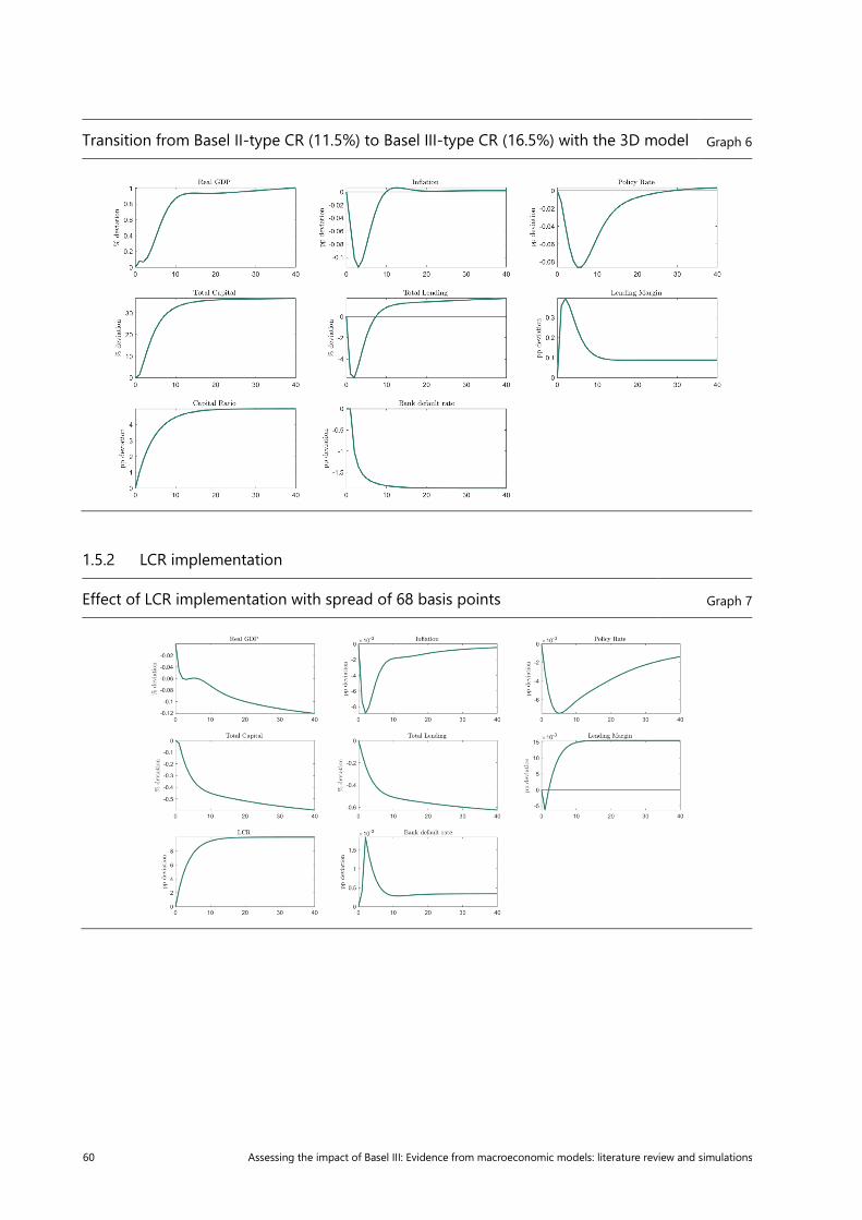
60 Assessing the impact of Basel III: Evidence from macroeconomic models: literature review and simulations
Transition from Basel II-type CR (11.5%) to Basel III-type CR (16.5%) with the 3D model Graph 6
1.5.2 LCR implementation
Effect of LCR implementation with spread of 68 basis points Graph 7

Assessing the impact of Basel III: Evidence from macroeconomic models: literature review and simulations 61
1.6 Response to shocks: Covid-19 scenario
Transitions following a -25% TFP shock and NFC default rate up to 15% Graph 8
2. Euro area analysis on the basis of de Bandt and Chahad (2016)29
2.1 Model specificities
The simulations are based on the model by de Bandt and Chahad (2016), in which the benefits of regulation are assessed by introducing the risk of bank run following Angeloni and Faia (2013). Bank run is the risk that depositors withdraw their deposits when banks are expected to fail. Due to a potent expectation channel, the reforms trigger quite rapidly a strong positive effect on GDP, as well as lending.
The asset side of banks includes sovereign bonds, corporate bonds, corporate loans and loans to SMEs. The liability side includes capital, deposits and interbank liabilities. The latter are not explicitly modelled as they offset each other at the aggregate level. However, regulation triggers substitution effects, as interbank liabilities are more runnable than household deposits.
2.2 Steady-state comparison
The direction of the change is similar to the simulations with the 3D model for solvency. In contrast, regarding the LCR, the effect is positive as the model includes the benefits of the regulation in terms of a lowering of the run probability. This generates positive expectations of future GDP growth.
29 By Olivier de Bandt (Bank of France) and Mohammed Chahad (European Central Bank and Bank of France).

62 Assessing the impact of Basel III: Evidence from macroeconomic models: literature review and simulations
2.2.1 Solvency
The impact of the reforms is positive, although the magnitude of the effect is relatively small. The direction of the change is similar to the simulations with the 3D model. Here the regulation implies a decrease in the probability of a run.30
Steady-state impact of a move from two different Basel II counterfactuals in the euro area (+2.5% pts and +5% pts capital ratios) to the current (Basel III) level of the bank capital ratio (16.5%) using the model by de Bandt and Chahad (2016) Table 11
Capital ratio
Bank PD
Bailout cost as % of GDP
Bank debt funding cost spread over risk-free rate
Bank lending rate to large firms
spread over bank debt fund. cost
Bank lending rate to SMEs spread over bank debt
fund. cost
GDP Aggregate investment
Aggr. cons.
Total lending to NFCs
2.5 -0.15 -0.01 -0.18 0.04 0.01 0.09 0.30 0.10 0.67
5 -0.29 -0.04 -0.34 0.08 0.02 0.18 0.56 0.18 1.26
% pts % pts % pts % pts % pts % pts % % % %
2.2.2 LCR
The scenario is slightly different from the one implemented with the other models, as the model allows taking into account the impact of the LCR on the reduction in run probability. As a consequence, through the expectation channel, GDP increases by 0.3% and lending to NFCs increases by 1.9%.
Steady-state impact of the implementation of a 100% LCR using the model by de Bandt and Chahad (2016) Table 12
LCR Bank PD
Bailout cost as % of GDP
Bank debt funding cost spread over risk-free rate
Bank lending rate to large firms
spread over bank debt fund. cost
Bank lending rate to SMEs spread over bank debt
fund. cost
GDP Aggregate investment
Aggr. cons.
Total lending to NFCs
+40 -0.68 -0.01 -0.61 0.20 0.11 0.27 0.28 0.87 1.94
% pts % pts % pts % pts % pts % pts % % % %
2.3 Transition to the new steady state
The graphs display the reaction over 10 years. In some cases, variables have not yet fully reached their final steady-state value, even if they are not far from it.
2.3.1 Solvency scenario
In many models, the implementation of solvency regulation leads to a short-run decrease in GDP and inflation, accommodated by monetary policy. Here, the transitory decline in GDP is rather short lived (a few quarters), slightly more pronounced when the capital ratio increases by 5 percentage points. The expectation of future growth stimulates demand, so that GDP and inflation are higher. Monetary policy reacts to inflation so that the transitory decline in inflation triggers a short-run decrease in interest rates,
30 Note that the levels of ratios are different from the ones displayed in the simulation with the 3D model for the euro area, where
the capital ratio includes additional voluntary buffers. But the simulation exercises are broadly comparable.
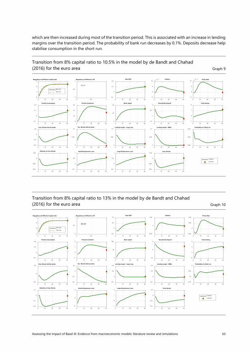
Assessing the impact of Basel III: Evidence from macroeconomic models: literature review and simulations 63
which are then increased during most of the transition period. This is associated with an increase in lending margins over the transition period. The probability of bank run decreases by 0.1%. Deposits decrease help stabilise consumption in the short run.
Transition from 8% capital ratio to 10.5% in the model by de Bandt and Chahad (2016) for the euro area Graph 9
Transition from 8% capital ratio to 13% in the model by de Bandt and Chahad (2016) for the euro area Graph 10
0 10 20 30 40
0
1
2
3Regulatory and Effective Capital ratio
Bank ratio
Reg. ratio
0 0.5 1
0
0.5
1Regulatory and Effective LCR
0 10 20 30 40
-0.1
0
0.1
0.2Real GDP
0 10 20 30 40
-5
0
5
1010 -3 Inflation
0 10 20 30 40
-5
0
5
1010 -3 Policy Rate
0 10 20 30 40
-0.1
0
0.1
0.2Private Consumption
0 10 20 30 40
0
0.2
0.4
0.6Private Investment
0 10 20 30 40
0
20
40Bank capital
0 10 20 30 40
-1.5
-1
-0.5
0Households Deposit
0 10 20 30 40
-1
0
1
2Total lending
0 10 20 30 40
-0.4
-0.2
0
0.2Corp. Bonds held by banks
0 10 20 30 40
0
0.05
0.1Sov. Bonds held by banks
0 10 20 30 40
0
0.05
0.1Lending margin - Large corp.
0 10 20 30 40
0
0.05
0.1Lending margin - SMEs
0 10 20 30 40
-0.06
-0.04
-0.02Probability of a Bank run
0 10 20 30 40
-0.04
-0.02
0
0.02Defaults on Corp. Bonds
0 10 20 30 40
-0.5
0
0.5
1Small Entrepreneur Loan
0 10 20 30 40
-0.5
0
0.5
1Large Entrepreneur Loan
0 10 20 30 40
-0.04
-0.02
0
0.02Corp. Bonds
Transitory
Long-term
NO LCR
0 10 20 30 40
0
2
4
6Regulatory and Effective Capital ratio
Bank ratio
Reg. ratio
0 0.5 1
0
0.5
1Regulatory and Effective LCR
0 10 20 30 40
-0.2
0
0.2
0.4Real GDP
0 10 20 30 40
-0.05
0
0.05Inflation
0 10 20 30 40
-0.02
0
0.02
0.04Policy Rate
0 10 20 30 40
-0.2
0
0.2
0.4Private Consumption
0 10 20 30 40
-1
0
1
2Private Investment
0 10 20 30 40
0
50
100Bank capital
0 10 20 30 40
-10
-5
0Households Deposit
0 10 20 30 40
-2
0
2
4Total lending
0 10 20 30 40
-0.5
0
0.5Corp. Bonds held by banks
0 10 20 30 40
-0.4
-0.2
0
0.2Sov. Bonds held by banks
0 10 20 30 40
-0.2
0
0.2
0.4Lending margin - Large corp.
0 10 20 30 40
-0.2
0
0.2
0.4Lending margin - SMEs
0 10 20 30 40
-0.15
-0.1
-0.05
0Probability of a Bank run
0 10 20 30 40
-0.2
-0.1
0
0.1Defaults on Corp. Bonds
0 10 20 30 40
-2
0
2Small Entrepreneur Loan
0 10 20 30 40
-1
0
1
2Large Entrepreneur Loan
0 10 20 30 40
-0.4
-0.2
0
0.2Corp. Bonds
Transitory
Long-term
NO LCR
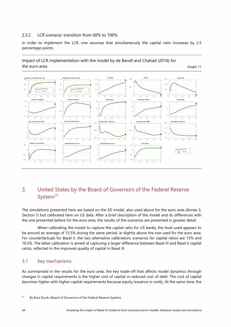
64 Assessing the impact of Basel III: Evidence from macroeconomic models: literature review and simulations
2.3.2 LCR scenario: transition from 60% to 100%
In order to implement the LCR, one assumes that simultaneously the capital ratio increases by 2.5 percentage points.
Impact of LCR implementation with the model by de Bandt and Chahad (2016) for the euro area Graph 11
3. United States by the Board of Governors of the Federal Reserve System31
The simulations presented here are based on the 3D model, also used above for the euro area (Annex 3, Section 1) but calibrated here on US data. After a brief description of the model and its differences with the one presented before for the euro area, the results of the scenarios are presented in greater detail.
When calibrating the model to capture the capital ratio for US banks, the level used appears to be around an average of 15.5% during the same period, ie slightly above the one used for the euro area. For counterfactuals for Basel II, the two alternative calibrations scenarios for capital ratios are 13% and 10.5%. The latter calibration is aimed at capturing a larger difference between Basel III and Basel II capital ratios, reflected in the improved quality of capital in Basel III.
3.1 Key mechanisms
As summarised in the results for the euro area, the key trade-off that affects model dynamics through changes in capital requirements is the higher cost of capital vs reduced cost of debt. The cost of capital becomes higher with higher capital requirements because equity issuance is costly. At the same time, the
31 By Bora Durdu (Board of Governors of the Federal Reserve System).
0 10 20 30 40
0
0.01
0.02
0.03Regulatory and Effective Cap. ratio
Effective Ratio
Reg. Ratio
0 10 20 30 40
0
0.2
0.4
0.6Regulatory and Effective LCR
Effective Ratio
Reg. Ratio
0 10 20 30 40
0
0.1
0.2
0.3Real GDP
0 10 20 30 40
0
0.01
0.02Inflation
0 10 20 30 40
0
0.01
0.02
0.03Policy Rate
0 10 20 30 40
-0.2
0
0.2
0.4Private Consumption
0 10 20 30 40
0
0.5
1
1.5Private Investment
0 10 20 30 40
0
20
40Bank capital
0 10 20 30 40
0
5
10
15Households Deposit
0 10 20 30 40
0
2
4Total lending
0 10 20 30 40
-4
-2
0
2Corp. Bonds held by banks
0 10 20 30 40
0
20
40Sov. Bonds held by banks
0 10 20 30 40
0.04
0.06
0.08Lending margin - Large corp.
0 10 20 30 40
0
0.05
0.1Lending margin - SMEs
0 10 20 30 40
-0.2
-0.15
-0.1
-0.05Probability of a Bank run
0 10 20 30 40
-0.02
-0.01
0
0.01Defaults on Corp. Bonds
0 10 20 30 40
0
1
2Small Entrepreneur Loan
0 10 20 30 40
0
1
2
3Large Entrepreneur Loan
0 10 20 30 40
-0.4
-0.2
0
0.2Corp. Bonds
Transitory
Long-term
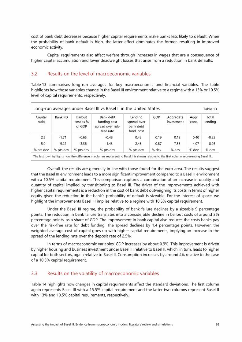
Assessing the impact of Basel III: Evidence from macroeconomic models: literature review and simulations 65
cost of bank debt decreases because higher capital requirements make banks less likely to default. When the probability of bank default is high, the latter effect dominates the former, resulting in improved economic activity.
Capital requirements also affect welfare through increases in wages that are a consequence of higher capital accumulation and lower deadweight losses that arise from a reduction in bank defaults.
3.2 Results on the level of macroeconomic variables
Table 13 summarises long-run averages for key macroeconomic and financial variables. The table highlights how those variables change in the Basel III environment relative to a regime with a 13% or 10.5% level of capital requirements, respectively.
Long-run averages under Basel III vs Basel II in the United States Table 13
Capital ratio
Bank PD Bailout cost as % of GDP
Bank debt funding cost
spread over risk-free rate
Lending spread over bank debt fund. cost
GDP Aggregate investment
Aggr. cons.
Total lending
2.5 -1.71 -0.65 -0.48 0.42 0.19 0.13 0.40 -0.22
5.0 -9.21 -3.36 -1.43 2.48 0.87 7.53 4.07 8.03
% pts dev % pts dev % pts dev % pts dev % pts dev % dev % dev % dev % dev
The last row highlights how the difference in columns representing Basel II is shown relative to the first column representing Basel III.
Overall, the results are generally in line with those found for the euro area. The results suggest that the Basel III environment leads to a more significant improvement compared to a Basel II environment with a 10.5% capital requirement. This comparison captures a combination of an increase in quality and quantity of capital implied by transitioning to Basel III. The driver of the improvements achieved with higher capital requirements is a reduction in the cost of bank debt outweighing its costs in terms of higher equity given the reduction in the bank’s probability of default is sizeable. For the interest of space, we highlight the improvements Basel III implies relative to a regime with 10.5% capital requirement.
Under the Basel III regime, the probability of bank failure declines by a sizeable 9 percentage points. The reduction in bank failure translates into a considerable decline in bailout costs of around 3¼ percentage points, as a share of GDP. The improvement in bank capital also reduces the costs banks pay over the risk-free rate for debt funding. The spread declines by 1.4 percentage points. However, the weighted-average cost of capital goes up with higher capital requirements, implying an increase in the spread of the lending rate over the deposit rate of 2.5%.
In terms of macroeconomic variables, GDP increases by about 0.9%. This improvement is driven by higher housing and business investment under Basel III relative to Basel II, which, in turn, leads to higher capital for both sectors, again relative to Basel II. Consumption increases by around 4% relative to the case of a 10.5% capital requirement.
3.3 Results on the volatility of macroeconomic variables
Table 14 highlights how changes in capital requirements affect the standard deviations. The first column again represents Basel III with a 15.5% capital requirement and the latter two columns represent Basel II with 13% and 10.5% capital requirements, respectively.

66 Assessing the impact of Basel III: Evidence from macroeconomic models: literature review and simulations
Standard deviations under Basel III vs Basel II Table 14
15.5% 13% 10.5%
GDP 2.96 3.03 3.30
Business investment 12.92 14.29 19.25
Housing investment 10.78 11.26 14.37
NFC loans-to-GDP ratio 2.45 2.75 3.99
Housing loans-to-GDP ratio 2.52 3.27 5.89
Avg. bank default 0.37 1.34 3.61
The volatility for virtually all variables moves down under Basel III, relative to Basel II with both levels of capital requirements. But the results are more significant when compared to the regime with a 10.5% capital requirement. The volatility of GDP goes down under Basel III, partly driven by a reduction in the volatility of investment, driven by lower volatility of lending supported by a more stable banking system. The volatility of consumption is also lower under Basel III compared to Basel II. The volatility of the probability of bank failure is also considerably lower under Basel III reflecting improved capital positions of banks. Under Basel III, the probability of bank failure is also more stable.
3.4 Transitions from Basel II to Basel III
Graph 12 shows the transition paths from Basel II to Basel III, shown as percent deviation from the initial steady state under Basel II. We assume that the transition to the new capital requirement is completed over 20 quarters. During the transition, business investment shoots up initially before gradually declining and settling at a higher level. Lending for residential investment declines in the short term because it takes a while for banks to issue new equity or to accumulate it through retained earnings.32 With bank capital being fixed in the short term, higher capital requirements lead to lower lending. Consumption of both savers and borrowers increases gradually, supported by increased economic activity and cheaper bank loans. GDP falls initially but gradually converges to settle at a higher level.
32 This explains the decrease in GDP, as the indicator used here is an “augmented” definition of GDP.

Assessing the impact of Basel III: Evidence from macroeconomic models: literature review and simulations 67
Transition from Basel II capital ratio of 10.5% to Basel III capital ratio of 15.5% Graph 12
3.5 Steady-state comparison with LCR requirement
Similar to the analysis with the 3D model for the euro area and the NEMO model for Norway, in this section we investigate the macroeconomic effects of the LCR regulation following Hoerova et al (2019).
We approximate an LCR of 100% by requiring the representative bank in the model to hold government bonds equal to 10% of total deposits. In order to simplify the analysis further, we assume that government bonds carry no risk weight in the capital regulation meaning that the LCR does not have any effect on the capital requirements for banks. If the return on HQLA does not meet the interest and non-interest costs of deposits required to finance the HQLA, banks’ profits are reduced by an amount that is equal to the difference between the former two. Following Hoerova et al (2019), we calculate this cost to be 10 basis points based on the US data.
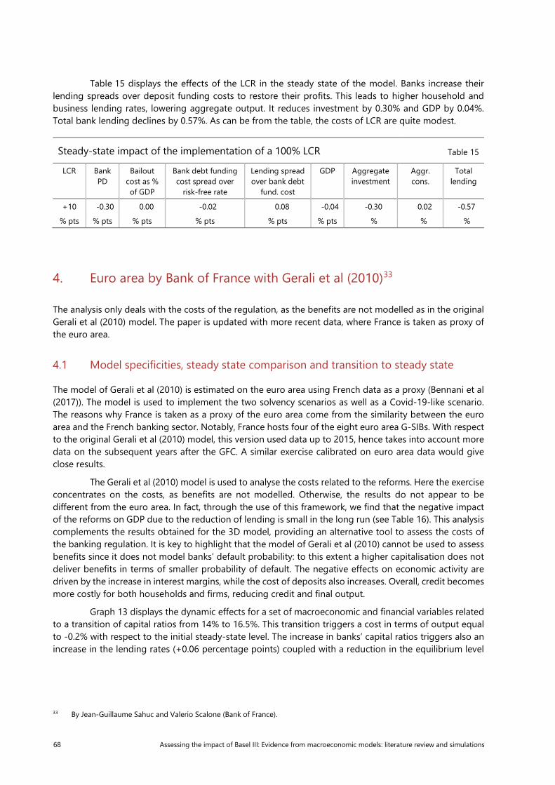
68 Assessing the impact of Basel III: Evidence from macroeconomic models: literature review and simulations
Table 15 displays the effects of the LCR in the steady state of the model. Banks increase their lending spreads over deposit funding costs to restore their profits. This leads to higher household and business lending rates, lowering aggregate output. It reduces investment by 0.30% and GDP by 0.04%. Total bank lending declines by 0.57%. As can be from the table, the costs of LCR are quite modest.
Steady-state impact of the implementation of a 100% LCR Table 15
LCR Bank PD
Bailout cost as % of GDP
Bank debt funding cost spread over
risk-free rate
Lending spread over bank debt
fund. cost
GDP Aggregate investment
Aggr. cons.
Total lending
+10 -0.30 0.00 -0.02 0.08 -0.04 -0.30 0.02 -0.57
% pts % pts % pts % pts % pts % pts % % %
4. Euro area by Bank of France with Gerali et al (2010)33
The analysis only deals with the costs of the regulation, as the benefits are not modelled as in the original Gerali et al (2010) model. The paper is updated with more recent data, where France is taken as proxy of the euro area.
4.1 Model specificities, steady state comparison and transition to steady state
The model of Gerali et al (2010) is estimated on the euro area using French data as a proxy (Bennani et al (2017)). The model is used to implement the two solvency scenarios as well as a Covid-19-like scenario. The reasons why France is taken as a proxy of the euro area come from the similarity between the euro area and the French banking sector. Notably, France hosts four of the eight euro area G-SIBs. With respect to the original Gerali et al (2010) model, this version used data up to 2015, hence takes into account more data on the subsequent years after the GFC. A similar exercise calibrated on euro area data would give close results.
The Gerali et al (2010) model is used to analyse the costs related to the reforms. Here the exercise concentrates on the costs, as benefits are not modelled. Otherwise, the results do not appear to be different from the euro area. In fact, through the use of this framework, we find that the negative impact of the reforms on GDP due to the reduction of lending is small in the long run (see Table 16). This analysis complements the results obtained for the 3D model, providing an alternative tool to assess the costs of the banking regulation. It is key to highlight that the model of Gerali et al (2010) cannot be used to assess benefits since it does not model banks’ default probability: to this extent a higher capitalisation does not deliver benefits in terms of smaller probability of default. The negative effects on economic activity are driven by the increase in interest margins, while the cost of deposits also increases. Overall, credit becomes more costly for both households and firms, reducing credit and final output.
Graph 13 displays the dynamic effects for a set of macroeconomic and financial variables related to a transition of capital ratios from 14% to 16.5%. This transition triggers a cost in terms of output equal to -0.2% with respect to the initial steady-state level. The increase in banks’ capital ratios triggers also an increase in the lending rates (+0.06 percentage points) coupled with a reduction in the equilibrium level
33 By Jean-Guillaume Sahuc and Valerio Scalone (Bank of France).

Assessing the impact of Basel III: Evidence from macroeconomic models: literature review and simulations 69
of total lending (-3%). These numbers are almost doubled in the case of a transition of capital ratios from 11.5% to 16.5% (Graph 14).
Long-run averages under Basel III vs Basel II in euro area (proxied by France) Table 16
Capital ratio
Bank PD
Bailout cost as % of GDP
Bank debt funding cost spread over risk-free rate
Lending spread over bank debt fund. cost
GDP Aggregate investment
Aggregate cons.
Total lending
+2.5 NaN NaN 0.09 0.06 -0.21 -0.68 -0.24 -3.07
+5.0 NaN NaN 0.17 0.11 -0.39 -1.31 -0.45 -5.85
% pts dev - - % pts dev % pts dev % dev % dev % dev % dev
The last row highlights how the difference in columns representing Basel II is shown relative to the first column representing Basel III.
Euro area (proxied by France): transition from Basel II capital ratio of 14% to Basel III capital ratios of 16.5% Graph 13

70 Assessing the impact of Basel III: Evidence from macroeconomic models: literature review and simulations
Euro area (proxied by France): transition from Basel II capital ratio of 11.5% to Basel III capital ratios of 16.5% Graph 14
4.2 Impact of Covid-19 scenario
Two simulations are implemented in order to replicate the Covid-19 crisis, characterised by an 8% drop in GDP. First, a pure TFP shock of six times the standard deviation of TFP, ie a persistent decrease of TFP by 14.4%. Second, a TFP by six standard deviations, ie a persistent decrease in TFP by 14.4%, combined with a decrease of investment by four standard deviations, or a drop by 27.6%.
In both scenarios, as calibrated, GDP drops by around 8%. Banks exhibit a cyclical reaction: in the short run, they increase interest on loans, which affects positively profits and capital. When the crisis materialises, interest rates decrease; the collateral channel leads to a reduction in loans and the capital ratio drops by 0.5 percentage points with a slightly more negative impact in the Basel III regime. However, the benefits of Basel III are a bit more visible for housing loans than for NFC loans. Indeed the reduction in housing loans is more significant in Basel II than in the two Basel III scenarios

Assessing the impact of Basel III: Evidence from macroeconomic models: literature review and simulations 71
Euro area (proxied by France) – scenario 1: pure TFP shock (-14.4%) Impulse responses to a TFP shock under different levels of CET1 ratios Graph 15
Euro area (proxied by France) – scenario 2: TFP (-7.2%) and investment (-27.6%) Impulse responses to TFP and investment shocks under different levels of CET1 ratios Graph 16
72 Assessing the impact of Basel III: Evidence from macroeconomic models: literature review and simulations
5. Norway by Central Bank of Norway34
The costs and benefits of transitioning to Basel III capital requirements in Norway are assessed using a Markov regime-switching version of NEMO, the main DSGE model used for policy analysis and forecasting by the Central Bank of Norway (Kravik and Mimir (2019), Kockerols et al (2021)). It explicitly takes into account the downside risks to GDP by considering the possibility of, and the severity of, endogenous financial crises due to credit imbalances. We also compare the two capital regimes along a certain number of criteria, in order to assess the net benefits of Basel III.
5.1 Model description
NEMO is a large-scale New Keynesian DSGE model of a small open economy. The economy consists of households, domestic intermediate-goods and final-goods firms, housing and non-housing capital goods producers, a banking sector, an oil sector and the monetary authority. All agents have rational, or model-consistent, expectations with respect to all prices and quantities, except for households’ house price expectations, which are partly backward looking, based on Gelain et al (2018). The model is estimated for the Norwegian economy with Bayesian methods.
The model features several real and nominal rigidities. These standard features are habit persistence, investment adjustment costs and variable capacity utilisation. Prices and wages are sticky. The model also includes collateral constraints based on loan-to-value ratios for households and entrepreneurs, long-term mortgage debt contracts, incomplete interest rate pass-through and capital requirements in the banking sector.
The banking sector in NEMO is built on Gerali et al (2010). Banks provide loans to both households and non-financial firms and fund themselves using household deposits, foreign borrowing and equity capital. They cannot raise outside equity. They set interest rates in a monopolistically competitive fashion subject to adjustment costs, which leads to imperfect and sluggish interest rate pass-through from the policy rate to loan and deposit rates. They choose the overall level of lending and funding, adhering to regulatory capital requirements adjusted for asset specific risk weights. Banks incur a quadratic cost if they fail to meet their capital-to-asset ratio target. Kravik and Mimir (2019) document the model in detail.
The regime-switching version of NEMO is built to incorporate endogenous financial crises stemming from persistently high credit growth (based on Gerdrup et al (2017)) as well as an endogenous zero lower bound (ZLB) on interest rates (based on Aruoba et al (2018)). A crisis can occur at any point in time governed by a two-state Markov process. The economy can be either in a normal state or in a crisis state. Business cycles in normal times are driven by the estimated typical shocks in the constant-parameter version of NEMO. Crisis times are driven by some structural changes in the domestic economy and asymmetric low-probability crisis shocks, which will be explained below. Moreover, the actual policy rate can hit the ZLB at any point in time governed by another two-state Markov process: no-ZLB vs ZLB. The actual policy rate is equal to the ZLB whenever the shadow policy rate implied by the simple policy rule goes into negative territory. Otherwise, the actual policy rate is equal to the shadow policy rate. The ZLB steady state is implemented by assuming a zero steady-state inflation rate. Taken together with the endogenous ZLB on interest rates, the economy can be either in one of the four following regimes at any point in time: no-crisis no-ZLB, no-crisis ZLB, crisis no-ZLB, and crisis-ZLB.
Following Gerdrup et al (2017) and Ajello et al (2019), we assume that economic agents in the model underestimate the probability of a crisis. In particular, they attach a zero probability to a crisis happening and hence do not internalise the effect of their borrowing decisions on the crisis probability.
34 By Yasin Mimir (Central Bank of Norway).
Assessing the impact of Basel III: Evidence from macroeconomic models: literature review and simulations 73
However, the policymaker, in principle, can consider this pecuniary externality while setting the optimal level of capital requirements.
Both the probability and the severity of crises are determined by five-year cumulative real household credit growth, which is found to be a robust indicator of financial vulnerabilities in Norway, predicting the downside risks to GDP (see Arbatli-Saxegaard et al (2020)). The probability of a crisis is estimated based on a sample of 20 OECD countries (see Gerdrup et al (2017)). When the economy endogenously enters into a crisis state, certain asymmetric shocks hit the economy and particular structural model parameters regarding the financial sector shift. These structural changes are especially related to the banking and housing sectors. First, the money market premium (the difference between the money market rate and the policy rate) and the external risk premium in the uncovered interest parity condition become more sensitive to changes in banks’ capital positions. Second, risk weights on loans to businesses and households increase. Finally, house prices and housing investment become more volatile. The economy is also hit by some crisis shocks. These are shocks to bank net worth, housing preferences, consumption preferences and the marginal efficiency of business investment. The shock to bank net worth represents a credit supply shock motivated by loan losses and asset write-downs. The shock to housing preferences represents a credit demand shock motivated by an adverse feedback loop between the deterioration in house prices and lower credit demand. The shock to consumption preferences represents an aggregate demand shock motivated by large growth in consumer loans. Finally, the shock to investment represents an aggregate supply shock motivated by a productivity slowdown observed during financial crises. The standard deviations of the asymmetric shocks and the shifting structural parameters in the crisis state are calibrated to roughly reflect the macroeconomic scenario used in the recent macroprudential stress testing analyses (see Central Bank of Norway (2019)). Kockerols et al (2021) document the Markov regime-switching version of the model in detail.
The parameterisation and modelling of endogenous financial crises in NEMO are presented in Annex 6.
5.2 The effects of capital requirements on real economic activity and welfare
The banking sector in NEMO is monopolistically competitive, following Gerali et al (2010). Banks set interest rates on deposits and on loans to maximise profits. Since NEMO is a small open economy model, the cost of foreign borrowing follows from an uncovered interest parity condition, depending on the foreign interest rate plus an external debt-elastic risk premium. The amount of loans issued by each bank can be financed through deposits, foreign borrowing and bank capital, which is accumulated through retained earnings. Moreover, banks are assumed to have a regulatory target for their risk-weighted capital-to-assets ratio. The deviations from this regulatory target imply a quadratic cost. They also target a specific level of return on equity based on different levels of regulatory capital requirements.
Banks set the interest rates on household and business loans as mark-ups over marginal cost of funding, which is a weighted average of the cost of deposits, foreign borrowing and the cost of equity (the cost of deviating from regulatory capital requirement). Banks pass the increases in the cost of funding to the interest rates on household and business loans. A higher cost of funding leads to higher lending spreads for households and firms.
A higher capital requirement leads to a larger deviation from the regulatory target, implying a higher quadratic cost for banks over the business cycle. The rise in the cost of equity generates an increase in the weighted average of funds for banks. As a result, lending spreads rise generating a reduction in lending to households and firms. This leads to lower business and residential investment, and hence lower real economic activity. The effect of higher capital requirements on consumption depends on real wages and dividends from bank profits. Although real wages are lower due to lower capital accumulation under higher capital requirements, the dividends to households coming from bank profits might be higher due to the increased lending spreads.
74 Assessing the impact of Basel III: Evidence from macroeconomic models: literature review and simulations
The other channel where changes in capital requirements affect the economy is through the probability of a crisis. Since the probability of a crisis depends on five-year real household credit growth, a higher level of capital requirements leads to a reduction in household credit growth and hence a fall in the crisis probability in a given business cycle upturn. A lower crisis probability means that the economy experiences a lower number of stress episodes, which is highly costly in terms of reduced output. In addition, the cost of crises in terms of reduced output is lower given a higher level of capital requirements. The reason is that for given loan losses, the reduction in the bank equity ratio is lower when banks have more capital. Therefore, the cost of deviation from the regulatory target is lower, leading to smaller increases in loan spreads and higher output.
Overall, the benefits of higher capital requirements are reduced crisis probability and lower cost of crisis while the costs are an increase in lending spreads and lower level of GDP in normal times. Depending on the relative magnitude of these benefits and costs, the ergodic mean of output might be higher or lower in response to an increase in the level of regulatory capital requirements.
Households’ welfare in the model depends on consumption, labour, housing services and deposits. The effect of changes in the capital requirements on welfare hinges on the relative impacts of different channels discussed above on those welfare components. On one hand, higher capital requirements can lead to higher consumption and deposits through higher spreads and higher bank profits but to lower hours worked and housing services. On the other hand, through the crisis probability channel, higher capital requirements reduce the crisis probability generating a higher consumption, hours worked, housing services and deposits.
5.3 Steady-state analysis of changes in capital requirements
Table 17 displays the deterministic steady-state values of the main macroeconomic and financial variables across different Basel frameworks. In particular, the first column tabulates the long-run values in levels under Basel III rules (with a 16.3% capital requirement), and the last two columns show those values under pre-Basel III (13.8% and 11.3%, respectively) as percent deviation or percentage point difference from moving from pre-Basel III to post-Basel III.
Table 17 shows that real GDP in the deterministic steady-state shrinks by 0.21% and 0.44% going from pre-Basel III regimes of 13.8% and 11.3% capital requirements to post-Basel III of 16.3% capital requirement, respectively. This result is mainly due to lower business, residential and oil investment resulting from higher lending margins and lower bank lending.
We must stress here that the deterministic steady-state comparisons of different capital requirement regimes do not reflect both the costs and benefits of changes in capital requirements at the same time. It only shows the costs of higher capital requirements in normal times but it does not reflect the benefits of higher capital requirements in terms of reducing crisis probability and the crisis severity. In order to see the benefits as well, we need to look at the ergodic means, which include the occurrence of crisis events. It might give us a different picture depending on the sensitivities of the crisis probability and the crisis severity to the degree of financial vulnerabilities in the economy.

Assessing the impact of Basel III: Evidence from macroeconomic models: literature review and simulations 75
Deterministic steady states of key macroeconomic and financial variables Table 17
Macro variables – steady state level Post-Basel III (SS levels) Post-Basel III/pre-Basel III
Under current TCR level (1) Current CR-2.5% (2) Current CR-5% (3)
Real GDP 4.57 -0.21 -0.44
Total investment 1.02 -2.03 -4.30
Business investment 0.41 -1.98 -4.19
Residential investment 0.32 -2.77 -5.89
Oil investment 0.28 -1.23 -2.63
Lending to NFC 15.26 -2.07 -4.38
Lending to HH 19.26 -2.77 -5.88
Total lending 34.52 -2.46 -5.21
Table 18 shows the ergodic means of the same macroeconomic and financial variables. Comparing the first column of Table 17 to that of Table 18 indicates that the crisis episodes reduce the level of output as well as the other main macroeconomic aggregates compared to their deterministic steady states. The level of real GDP is 4.57 in the deterministic steady state while its ergodic mean is 4.54, reflecting the cost of crises. Moreover, Table 18 shows that the ergodic mean of real GDP falls by 0.14% and 0.18% going from pre-Basel III regimes to post-Basel III compared to 0.21% and 0.44% in the deterministic steady state, respectively. This implies that the post-Basel III capital regime reduces the cost of crisis events and the crisis probability compared to pre-Basel III capital regimes, leading to a lower fall in output compared to the deterministic steady state.
Table 18 also displays the crisis probabilities under different capital regimes. The annualised probability of a crisis under the post-Basel III regime is 3.38% while those under pre-Basel III regimes of 13.8% and 11.3% capital requirements are 3.45% and 3.54%, respectively. The crisis probability falls as the capital requirements increase due to the decline in the volatility of household credit. However, the reduction in the crisis probability is not large. This result is consistent with Jorda et al (2017), which shows that higher capital requirements do not substantially reduce the crisis probability but reduce the cost of crises.
Ergodic means of key macroeconomic and financial variables Table 18
Macro variables – ergodic means1 Post-Basel III (SS Levels) Post-Basel III/Pre-Basel III
Under Current TCR level (1) Current CR-2.5% (2) Current CR-5% (3)
Real GDP 4.54 -0.14 -0.18
Total investment 0.72 -1.77 -2.96
Business investment 0.41 -1.59 -3.02
Residential investment 0.31 -1.99 -2.85
Oil investment 0.28 -1.18 -2.68
Lending to NFC 14.83 -1.66 -3.15
Lending to HH 18.74 -2.05 -3.20
Total lending 33.58 -1.88 -3.18
Probability of a financial crisis (%) 3.38 -0.07 -0.16 1 Ergodic means of macroeconomic and financial variables differ from their deterministic steady-state values due to the occurrence of crisis events.

76 Assessing the impact of Basel III: Evidence from macroeconomic models: literature review and simulations
Graph 17 displays the average crisis behaviour of some selected macroeconomic variables under different capital requirement regimes. It shows the cost of crisis events under pre-Basel III and post-Basel III capital regimes. It indicates that the decline in the output gap is slightly lower under a 16.3% capital requirement compared to a 13.8% capital requirement but is substantially lower than that under an 11.3% capital requirement in terms of cumulative output losses. Overall, the cost of crises is higher under an 11.3% capital requirement compared to 13.8% and 16.3% capital requirements, but it is not too different across the latter two regimes. We would like to note that the results depend on the sensitivities of the crisis severity and the crisis probability to real household credit growth. An additional experiment below shows that higher capital requirements are more beneficial when those sensitivities to credit growth are higher.
Average crisis behaviour of macroeconomic variables across different capital requirement regimes Graph 17
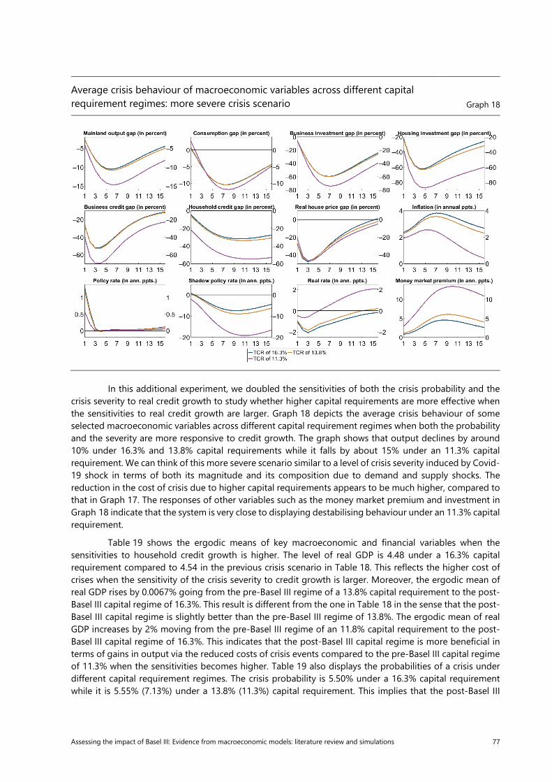
Assessing the impact of Basel III: Evidence from macroeconomic models: literature review and simulations 77
Average crisis behaviour of macroeconomic variables across different capital requirement regimes: more severe crisis scenario Graph 18
In this additional experiment, we doubled the sensitivities of both the crisis probability and the crisis severity to real credit growth to study whether higher capital requirements are more effective when the sensitivities to real credit growth are larger. Graph 18 depicts the average crisis behaviour of some selected macroeconomic variables across different capital requirement regimes when both the probability and the severity are more responsive to credit growth. The graph shows that output declines by around 10% under 16.3% and 13.8% capital requirements while it falls by about 15% under an 11.3% capital requirement. We can think of this more severe scenario similar to a level of crisis severity induced by Covid-19 shock in terms of both its magnitude and its composition due to demand and supply shocks. The reduction in the cost of crisis due to higher capital requirements appears to be much higher, compared to that in Graph 17. The responses of other variables such as the money market premium and investment in Graph 18 indicate that the system is very close to displaying destabilising behaviour under an 11.3% capital requirement.
Table 19 shows the ergodic means of key macroeconomic and financial variables when the sensitivities to household credit growth is higher. The level of real GDP is 4.48 under a 16.3% capital requirement compared to 4.54 in the previous crisis scenario in Table 18. This reflects the higher cost of crises when the sensitivity of the crisis severity to credit growth is larger. Moreover, the ergodic mean of real GDP rises by 0.0067% going from the pre-Basel III regime of a 13.8% capital requirement to the post-Basel III capital regime of 16.3%. This result is different from the one in Table 18 in the sense that the post-Basel III capital regime is slightly better than the pre-Basel III regime of 13.8%. The ergodic mean of real GDP increases by 2% moving from the pre-Basel III regime of an 11.8% capital requirement to the post-Basel III capital regime of 16.3%. This indicates that the post-Basel III capital regime is more beneficial in terms of gains in output via the reduced costs of crisis events compared to the pre-Basel III capital regime of 11.3% when the sensitivities becomes higher. Table 19 also displays the probabilities of a crisis under different capital requirement regimes. The crisis probability is 5.50% under a 16.3% capital requirement while it is 5.55% (7.13%) under a 13.8% (11.3%) capital requirement. This implies that the post-Basel III

78 Assessing the impact of Basel III: Evidence from macroeconomic models: literature review and simulations
capital regime is more effective in reducing the crisis probability compared to the pre-Basel III capital regimes when the sensitivities to credit growth are bigger.
Ergodic means of key macroeconomic and financial variables under a more severe crisis scenario Table 19
Macro variables – ergodic means1 Post-Basel III (SS levels) Post-Basel III/pre-Basel III
Under current TCR level (1) Current CR-2.5% (2) Current CR-5% (3)
Real GDP 4.48 0.007 2.10
Total investment 0.68 -0.68 12.43
Business investment 0.38 -0.99 6.52
Residential investment 0.29 -0.28 20.26
Oil investment 0.29 -1.26 -4.64
Lending to NFC 13.82 -1.07 8.10
Lending to HH 17.55 -0.59 16.72
Total lending 31.37 -0.80 12.92
Probability of a financial crisis (%) 5.50 -0.05 -1.63 1 Ergodic means of macroeconomic and financial variables differ from their deterministic steady-state values due to the occurrence of crisis events.
Table 20 summarises the benefits and costs of different capital regimes. Overall, the results seem to be consistent with the costs and benefits analysis of bank capital in BCBS (2019). The deterministic steady-state comparisons show that higher capital requirements under post-Basel III, and thus higher costs for banks, lead to an increase in loan spreads, a fall in bank lending and hence a decline in real GDP. When we take into account the benefits of higher requirements, such as reduced crisis probability and lower cost of crisis in terms of real GDP through the ergodic mean comparisons, higher capital requirements under post-Basel III become more beneficial. When the sensitivities of the crisis probability and the crisis severity to real household credit growth are sufficiently large, the ergodic mean of real GDP is 2% higher under post-Basel III compared to pre-Basel III capital regime of 11.3%. The crisis probability is also 1.63 percentage points lower under the post-Basel III regime compared to pre-Basel capital regime of 11.3%.
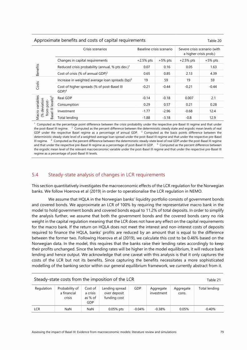
Assessing the impact of Basel III: Evidence from macroeconomic models: literature review and simulations 79
5.4 Steady-state analysis of changes in LCR requirements
This section quantitatively investigates the macroeconomic effects of the LCR regulation for the Norwegian banks. We follow Hoerova et al (2019) in order to operationalise the LCR regulation in NEMO.
We assume that HQLA in the Norwegian banks’ liquidity portfolio consists of government bonds and covered bonds. We approximate an LCR of 100% by requiring the representative macro bank in the model to hold government bonds and covered bonds equal to 11.2% of total deposits. In order to simplify the analysis further, we assume that both the government bonds and the covered bonds carry no risk weight in the capital regulation meaning that the LCR does not have any effect on the capital requirements for the macro bank. If the return on HQLA does not meet the interest and non-interest costs of deposits required to finance the HQLA, banks’ profits are reduced by an amount that is equal to the difference between the former two. Following Hoerova et al (2019), we calculate this cost to be 0.46% based on the Norwegian data. In the model, this requires that the banks raise their lending rates accordingly to keep their profits unchanged. Since the lending rates will be higher in the model equilibrium, it will reduce bank lending and hence output. We acknowledge that one caveat with this analysis is that it only captures the costs of the LCR but not its benefits. Since capturing the benefits necessitates a more sophisticated modelling of the banking sector within our general equilibrium framework, we currently abstract from it.
Steady-state costs from the imposition of the LCR Table 21
Regulation Probability of a financial
crisis
Cost of a crisis as % of
GDP
Lending spread over deposit funding cost
GDP Aggregate investment
Aggregate cons.
Total lending
LCR NaN NaN 0.05% pts -0.04% -0.38% 0.05% -0.40%
Approximate benefits and costs of capital requirements Table 20
Crisis scenarios Baseline crisis scenario Severe crisis scenario (with a higher crisis prob.)
Changes in capital requirements +2.5% pts +5% pts +2.5% pts +5% pts
Bene
fits
Reduced crisis probability (annual, % pts dev.)1 0.07 0.16 0.05 1.63
Cost of crisis (% of annual GDP)2 0.65 0.85 2.13 4.39
Cost
s Increase in weighted average loan spreads (bp)3 19 59 19 59
Cost of higher spreads (% of post-Basel III GDP)4
-0.21 -0.44 -0.21 -0.44
Mac
ro v
aria
bles
(%
dev
iatio
n fro
m p
ost-
Ba
sel I
II le
vels)
5
Real GDP -0.14 -0.18 0.007 2.1
Consumption 0.29 0.57 0.21 0.28
Investment -1.77 -2.96 -0.68 12.4
Total lending -1.88 -3.18 -0.8 12.9 1 Computed as the percentage point difference between the crisis probability under the respective pre-Basel III regime and that under the post-Basel III regime. 2 Computed as the percent difference between the deterministic steady state and ergodic mean levels of real GDP under the respective Basel regime as a percentage of annual GDP. 3 Computed as the basis points difference between the deterministic steady-state level of a weighted-average loan spread under the post-Basel III regime and that under the respective pre-Basel III regime. 4 Computed as the percent difference between the deterministic steady-state level of real GDP under the post-Basel III regime and that under the respective pre-Basel III regime as a percentage of post-Basel III GDP. 5 Computed as the percent difference between the ergodic mean level of the relevant macroeconomic variable under the post-Basel III regime and that under the respective pre-Basel III regime as a percentage of post-Basel III levels.

80 Assessing the impact of Basel III: Evidence from macroeconomic models: literature review and simulations
Table 21 displays the macroeconomic effects of the LCR in the steady state of the model. Banks increase their lending spreads over deposit funding costs by 5.1 basis points (the cost of holding one more unit of HQLA of 0.46% multiplied by the share of HQLA in total deposits of 11.2%) to restore their profits. This leads to higher household and business lending rates, lowering aggregate output. It reduces investment by 0.38% and GDP by 0.04% only (as consumption goes up; since households benefit as shareholders from higher bank profits). Total bank lending declines by 0.40%. The analysis shows that the costs of the LCR are quite modest compared to its potential benefits during a possible liquidity crisis. Below, we also provide the transitional impact of the LCR from an environment with no LCR to one with the LCR.
5.5 Transitions from Basel II to Basel III
5.5.1 Transition to solvency requirements
Graph 19 (in levels) and Graph 20 (in per cent change with respect to initial steady state) display the transition path from a deterministic steady state under a pre-Basel III regime of 13.8% capital requirements (intercept on the y-axis) to that under a post-Basel III regime of 16.3% capital requirements (orange line). Bank capital to total assets mostly completes its transition in 20 quarters (the blue line mostly converges to the orange line for the ratio of bank capital to risk-weighted assets in 20 quarters). The transition in other macroeconomic variables takes much longer than 20 quarters due to the endogenous propagation in the model.
Transition from a TCR of 13.8% in pre-Basel III regime to a TCR of 16.3% in post-Basel III regime In levels Graph 19

Assessing the impact of Basel III: Evidence from macroeconomic models: literature review and simulations 81
Transition from a TCR of 13.8% in pre-Basel III regime to a TCR of 16.3% in post-Basel III regime In percent deviation from initial steady state Graph 20
The figures show that real GDP falls sharply in earlier periods and then converges to a slightly lower level under the new regime. The reason is that both lending margins display a sharp increase in the first five quarters and converge to higher levels than their initial steady state. Total lending shows a similar but more gradual behaviour. The central bank reduces the policy rate to accommodate the decline in GDP but then raises it to its initial value as the output recovers. Annual inflation first rises due to an exchange rate depreciation caused by a lower policy rate. It then falls as domestic demand shrinks but converges to its initial steady-state value. Overall, inflation and the policy rate do not change in the deterministic steady state.
Graph 21 and Graph 22 show the transition path from a deterministic steady state under a pre-Basel III regime of 11.3% capital requirements to that under a post-Basel III regime of 16.3% capital requirements. The macroeconomic and financial aggregates display similar behaviour as in the previous figures albeit slightly sharper due to a bigger change in the regulatory capital requirements.

82 Assessing the impact of Basel III: Evidence from macroeconomic models: literature review and simulations
Transition from a TCR of 11.3% in pre-Basel III regime to a TCR of 16.3% in post-Basel III regime In levels Graph 21
Transition from a TCR of 11.3% in pre-Basel III regime to a TCR of 16.3% in post-Basel III regime In percent deviation from initial steady state Graph 22

Assessing the impact of Basel III: Evidence from macroeconomic models: literature review and simulations 83
5.5.2 Transition to LCR requirements
Transition to a 100% LCR requirement In levels Graph 23
Transition to a 100% LCR requirement In percent deviation from initial steady state Graph 24

84 Assessing the impact of Basel III: Evidence from macroeconomic models: literature review and simulations
5.6 Business cycle moments: Basel II vs Basel III comparison
Table 22 shows the second order moments of main macroeconomic and financial variables across different Basel capital requirement regimes. The numbers in all columns represent the level of standard deviations in post- and pre-Basel III accords. The results show that higher capital requirements under Basel III lead to lower volatilities in main macroeconomic aggregates such as real GDP, consumption and investment. This also holds for financial variables.
Business cycle moments of key macroeconomic and financial variables In per cent Table 22
Macro variables – second moments Post-Basel III Post-Basel III/pre-Basel III
Under current TCR level (1) Current CR-2.5% (2) Current CR-5% (3)
Real GDP 1.94 2.01 2.37
Total investment 12.20 12.48 14.47
Business investment 16.45 16.71 17.97
Residential investment 16.83 16.96 19.45
Oil investment 11.58 11.60 11.78
Lending to HH 12.42 12.51 14.47
Lending to NFC 10.14 10.25 11.12
Total lending 7.94 8.10 9.68
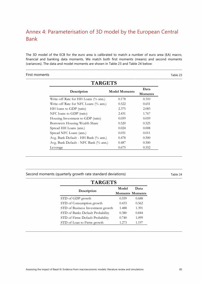
Assessing the impact of Basel III: Evidence from macroeconomic models: literature review and simulations 85
Annex 4: Parameterisation of 3D model by the European Central Bank
The 3D model of the ECB for the euro area is calibrated to match a number of euro area (EA) macro, financial and banking data moments. We match both first moments (means) and second moments (variances). The data and model moments are shown in Table 23 and Table 24 below:
First moments Table 23
Second moments (quarterly growth rate standard deviations) Table 24
Write-off Rate for HH Loans (% ann.) 0.178 0.310Write-off Rate for NFC Loans (% ann.) 0.522 0.651HH loans to GDP (ratio) 2.375 2.083NFC loans to GDP (ratio) 2.431 1.767Housing Investment to GDP (ratio) 0.059 0.059Borrowers Housing Wealth Share 0.520 0.525Spread HH Loans (ann.) 0.024 0.008Spread NFC Loans (ann.) 0.031 0.011Avg. Bank Default - HH Bank (% ann.) 0.478 0.500Avg. Bank Default - NFC Bank (% ann.) 0.487 0.500Leverage 0.675 0.552
TARGETSDescription Model Moments
Data Moments
STD of GDP growth 0.559 0.688STD of Consumption growth 0.433 0.562STD of Business Investment growth 1.488 1.391STD of Banks Default Probability 0.380 0.844STD of Firms Default Probability 0.740 1.099STD of Loan to Firms growth 1.273 1.197
TARGETSDescription
Model Moments
Data Moments

86 Assessing the impact of Basel III: Evidence from macroeconomic models: literature review and simulations
Annex 5: Parameterisation of 3D model by the Board of Governors of the Federal Reserve System
Table 25 presents the calibration of the model and Table 26 summarises how the model performs in matching a set of targets.
Calibration Table 25
Data targets and steady-state values Table 26
Target Data Steady state
Write-off rate for HH loans (% ann) 0.43 0.20
Write-off rate for NFC loans (% ann) 2.73 0.82
HH loans to GDP (ratio) 0.57 1.84
NFC loans to GDP (ratio) 3.90 3.63
Housing Investment to GDP (ratio) 0.05 0.07
Average bank default 0.50 0.50
Leverage 1.43 1.10
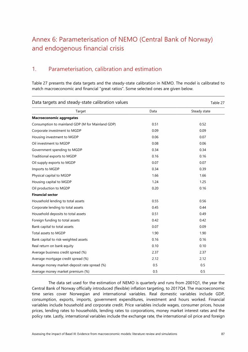
Assessing the impact of Basel III: Evidence from macroeconomic models: literature review and simulations 87
Annex 6: Parameterisation of NEMO (Central Bank of Norway) and endogenous financial crisis
1. Parameterisation, calibration and estimation
Table 27 presents the data targets and the steady-state calibration in NEMO. The model is calibrated to match macroeconomic and financial “great ratios”. Some selected ones are given below.
Data targets and steady-state calibration values Table 27
Target Data Steady state
Macroeconomic aggregates
Consumption to mainland GDP (M for Mainland GDP) 0.51 0.52
Corporate investment to MGDP 0.09 0.09
Housing investment to MGDP 0.06 0.07
Oil investment to MGDP 0.08 0.06
Government spending to MGDP 0.34 0.34
Traditional exports to MGDP 0.16 0.16
Oil supply exports to MGDP 0.07 0.07
Imports to MGDP 0.34 0.39
Physical capital to MGDP 1.66 1.66
Housing capital to MGDP 1.24 1.25
Oil production to MGDP 0.20 0.16
Financial sector
Household lending to total assets 0.55 0.56
Corporate lending to total assets 0.45 0.44
Household deposits to total assets 0.51 0.49
Foreign funding to total assets 0.42 0.42
Bank capital to total assets 0.07 0.09
Total assets to MGDP 1.90 1.90
Bank capital to risk-weighted assets 0.16 0.16
Real return on bank equity 0.10 0.10
Average business credit spread (%) 2.37 2.37
Average mortgage credit spread (%) 2.12 2.12
Average money market-deposit rate spread (%) 0.5 0.5
Average money market premium (%) 0.5 0.5
The data set used for the estimation of NEMO is quarterly and runs from 2001Q1, the year the Central Bank of Norway officially introduced (flexible) inflation targeting, to 2017Q4. The macroeconomic time series cover Norwegian and international variables. Real domestic variables include GDP, consumption, exports, imports, government expenditures, investment and hours worked. Financial variables include household and corporate credit. Price variables include wages, consumer prices, house prices, lending rates to households, lending rates to corporations, money market interest rates and the policy rate. Lastly, international variables include the exchange rate, the international oil price and foreign

88 Assessing the impact of Basel III: Evidence from macroeconomic models: literature review and simulations
GDP, money market rates and inflation. The data sources include Statistics Norway, Central Bank of Norway’s own calculations and international sources, particularly the IMF and Thomson Reuters. The data for the real variables are in constant prices from the national accounts, whereas credit and house prices are deflated by consumer prices. In total, there are 26 observable variables used in the estimation of NEMO. We use pre-filtered gap series (ie log-deviations from trend) when we estimate the model.
Table 28 displays the model-implied theoretical standard deviations of the observable variables used in the estimation of NEMO together with their empirical counterparts. The model-implied theoretical standard deviations are computed at the posterior mode.
Standard deviations of data vs model variables In per cent Table 28
Variable Data NEMO
Real variables
Mainland output 1.33 1.24
Consumption 1.23 1.82
Business investment 10.17 11.62
Housing investment 5.70 6.56
Oil investment 11.29 10.91
Government spending 0.77 0.94
Hours worked 1.51 1.45
Financial variables
Household credit 7.50 7.18
Business credit 4.95 5.72
Real house prices 4.28 6.06
Household lending rate 0.39 0.38
Corporate lending rate 0.37 0.39
External variables
Real effective exchange rate 5.40 4.65
Exports 2.81 3.43
Oil supply goods exports 5.16 5.74
Imports 3.36 2.72
Real oil prices 19.68 19.25
Trading partners’ output 3.91 3.33
Global output 1.04 0.77
Nominal variables
Aggregate inflation 0.29 0.24
Imported price inflation 0.45 0.48
Wage inflation 0.35 0.30
Policy rate 0.46 0.36
Money market rate abroad 0.48 0.35

Assessing the impact of Basel III: Evidence from macroeconomic models: literature review and simulations 89
2. Endogenous financial crises in NEMO
Graph 25 shows how the economy behaves on average when it enters into a crisis. In addition to estimated business cycle shocks, the economy is also hit by asymmetric large crisis shocks, ie shocks to bank capital, housing preferences, domestic consumption demand and marginal efficiency of investment. Due to the structural changes in the banking and housing sectors as well, those sectors also become more sensitive to these shocks. Since the changes in banks’ capital positions during crises endogenously affect the money market premium, altering the cost of funds for banks, a shock to bank capital leads to a 200 basis points increase in the premium. As a result, lending spreads also rise about 200 basis points in annual terms. This causes household credit and business credit to decline by about 15% and 25%, respectively. Hence business and housing investments decline by around 30% while mainland output and consumption fall by about 5% and 6%, respectively. The inflation rate first increases from 2.5% to almost 3.5% in the first eight quarters as the exchange rate depreciates. It then decreases by 0.6 percentage points to 2.8%. The shadow policy rate falls by almost 4 percentage points in annualised terms, going into negative territory. Due to the ZLB on nominal policy rate, it stays in the positive region, putting a drag on the economy.
Average behaviour of main macroeconomic variables in a financial crisis Graph 25
Graph 26 displays the average behaviour of the main macroeconomic variables during crises. We can also study different percentiles of these variables to see the dispersion of the severity of different crises. To this end, we simulate the model economy for 100,000 periods. We then collect the crisis events in these simulations. The number of crisis events is 800. Graph 26 shows 30th, 50th, 70th and 90th percentiles of different variables across these 800 crises. In the least severe crisis, output falls by about 2% at the peak while it declines by around 9% in the most severe crisis. Depending on the severity, consumption, business and housing investments could fall by about 10%, 60% and 45%, respectively. The shadow policy rate could go down as much as 7% in annualised terms while the real rate could decline by 4%. In the worst possible crisis, the money market premium can sharply increase up to 600 basis points in annualised terms given the decline in bank capital.

90 Assessing the impact of Basel III: Evidence from macroeconomic models: literature review and simulations
Different percentiles of main macroeconomic variables in a financial crisis Graph 26
Graph 27 shows the distributions (kernel densities) of the output gap in the models with no crisis but ZLB (solid blue line), with crisis and no-ZLB (red dashed line), and with crisis and ZLB (solid yellow line), respectively. As expected, the distribution of the output gap in the model without a crisis is symmetric around zero, indicating no asymmetric tail risks either for the upside or for the downside. The left fat tail in the distribution under crisis but no ZLB displays significant downside risks to GDP while there are no upside risks. This is expected given the negative asymmetric crisis shocks and regime-switching structural parameters in the housing and banking sectors. Finally, the distribution of the output gap under crisis and ZLB regime reflects even more downside risks to GDP due to the policy rate hitting the ZLB. As the central bank has limited room for manoeuvre, it could not stimulate the economy as much as the case without the ZLB. The results are also in line with the GaR literature pioneered by Adrian et al (2019) showing how current financial conditions can affect downside risks to GDP growth (see also Arbatli-Saxegaard et al (2020) for GaR analysis for Norway).
We also compute the time spent in each regime over the business cycle. We find that the economy spends 76% of the time in the no crisis-no ZLB regime. This shows that more than three quarters of the time the economy evolves around typical business cycle fluctuations meaning that the estimated typical business cycle shocks do not lead the economy to experience either crisis or ZLB episodes. The simulations also show that 17% of the time is spent in the no crisis-ZLB regime. This is consistent with the unconditional probability of being in the ZLB regime estimated for the US economy by Aruoba et al (2017). This number indicates that given a 3% nominal policy rate in normal times, the estimated business cycle shocks tip the economy into the ZLB 17% of the time. It shows that given the low level of interest rates going forward, we might expect that ZLB episodes will be more frequent compared to the past. Moreover, we observe that the economy spends 3% of the time in the crisis-no ZLB regime and 4% of the time in crisis-ZLB regime. The former indicates that the effects of some of the simulated crises on inflation and output are not severe enough to lead the central bank to reduce the policy to the ZLB.
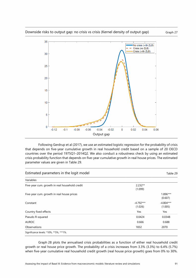
Assessing the impact of Basel III: Evidence from macroeconomic models: literature review and simulations 91
Downside risks to output gap: no crisis vs crisis (Kernel density of output gap) Graph 27
Output gap
Following Gerdrup et al (2017), we use an estimated logistic regression for the probability of crisis that depends on five-year cumulative growth in real household credit based on a sample of 20 OECD countries over the period 1975Q1–2014Q2. We also conduct a robustness check by using an estimated crisis probability function that depends on five-year cumulative growth in real house prices. The estimated parameter values are given in Table 29.
Estimated parameters in the logit model Table 29
Variables
Five-year cum. growth in real household credit 2.232** (1.099)
Five-year cum. growth in real house prices 1.896*** (0.607)
Constant -4.792*** (1.026)
-4.804*** (1.005)
Country fixed effects Yes Yes
Pseudo R-squared 0.0424 0.0348
AUROC 0.666 0.688
Observations 1832 2070
Significance levels: *10%, **5%, ***1%.
Graph 28 plots the annualised crisis probabilities as a function of either real household credit growth or real house price growth. The probability of a crisis increases from 3.3% (3.3%) to 6.4% (5.7%) when five-year cumulative real household credit growth (real house price growth) goes from 0% to 30%.
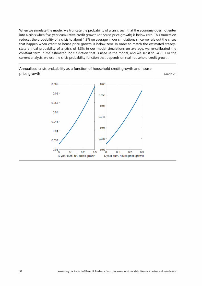
92 Assessing the impact of Basel III: Evidence from macroeconomic models: literature review and simulations
When we simulate the model, we truncate the probability of a crisis such that the economy does not enter into a crisis when five-year cumulative credit growth (or house price growth) is below zero. This truncation reduces the probability of a crisis to about 1.9% on average in our simulations since we rule out the crises that happen when credit or house price growth is below zero. In order to match the estimated steady-state annual probability of a crisis of 3.3% in our model simulations on average, we re-calibrated the constant term in the estimated logit function that is used in the model, and we set it to -4.25. For the current analysis, we use the crisis probability function that depends on real household credit growth.
Annualised crisis probability as a function of household credit growth and house price growth Graph 28