With Respect to the - NASA · elements of the planets and the planet pole vectors are ... coordinates with respect to the mean Earth equator and equinox of 1950.0

N A T I O N A L A E R O N A U T I C S A N D SPACE A D M I N I S T R A T I O N

Technical Report 32-7508

Polynomial Expressions for Planetary Equators and Orbit Elements With Respect to the

Mean 7950.0 Coordinate System

Francis M. Sturms, Jr.

J E T P R O P U L S I O N L A B O R A T O R Y C A L I F O R N I A I N S T I T U T E OF T E C H N O L O G Y

P A S A D E N A , C A L I F O R N I A

January 15, 1971

https://ntrs.nasa.gov/search.jsp?R=19710007310 2018-09-05T05:03:24+00:00Z

California Institute of Technology 5 4800 Oak Grove Drive, Pasadena, California 91103

October 13, 1971

Recipients of J e t Propulsion Laboratory Technical Report 32-1 508

Subject: Errata

Gentlemen:

Please note the following correct ions to Technical Report 32-1 508, Polynomial Expressions for Planetary Equators and Orbit Elements With Respect to the Mean 1950.0 Coordinate System, by Franc is M. Sturms, Jr. , dated January 15, 1971. should read as follows:

The values in Table 2 on page 7 of the report

Q = 98.02255 50

= -68.98877 %O

2 A50 = 180.28229 t 0. 11043 T t 0.00062 T

2 I 176. 54704 - 0.01507 T t 0.00001 T

Very t ruly yours ,

V John Kempton, Manager Publications Section

Telephone 354-4321 TWX 213-449-2451

N A T I O N A L A E R O N A U T I C S A N D SPACE A D M I N I S T R A T I O N

Francis M. Sfurms, Jr.

v C A L I F O R N I A I N S T I T U T E O F T E C H N O L O G Y

P A S A D E N A , C A L I FO R N I A

January 15, 1971

Prepared U n d e r Cont rac t No. N A S 7-1 00 N a t i o n a l Aeronaut ics a n d S p a c e Admin is t ra t ion

The work described in this report was performed by the Mission Analysis Division of the Jet Propulsion Laboratory.

iii

iv

wle t

The author wishes to express his thanks to Mrs. Helen Ling for her assistance in generating the data and polynomial curve fits for the report, and to Mr. Jack Hudes, a part-time UCLA student-employee, who performed the analysis and computations presented in Appendix A. Special thanks go to Miss Dorothy Babcock for her excellent typing of the manuscript.

JPL TECH~ICAL REPORT 32-1508

. . . . . . . . . . . . . . . . 1

nits of Time . . . . . . . . . . 2

olynomials . . . . . . . . . 2

A . Least-Squares Curve-Fit Method . . . . . . . . . . 3

B . Series Manipulation Method . . . . . . . . . . . 4

IV . Derivation of the Planet Equator Equations . . . . . . . . 4

V . Numerical Results . . . . . . . . . . . . . . 6

Appendix A . Consistency of Adopted Expressions for Precession Angles . . . . . . . . . . . . . . 10

Appendix 8 . Formulas for Series Manipulations . . . . . . . . 13

Appendix C . Coordinate System Transformations . . . . . . . 15

Appendix D . Special Treatment for Moon Angles . . . . . . . 18

Nomenclature . . . . . . . . . . . . . . . . . 20

References . . . . . . . . . . . . . . . . . . 22

Tables

1 . Mean orbit elements and north pole for Mercury

2 . Mean orbit elements and north pole for Venus . 3 . Mean orbit elements and north pole for Earth . 4 . Mean orbit elements and north pole for Mars . 5 . Mean orbit elements and north pole for Jupiter . 6 . Mean orbit elements and north pole for Saturn . 7 . Mean orbit elements and north pole for Uranus . 8 . Mean orbit elements and north pole for Neptune

9 . Mean orbit elements and north pole for Pluto

.

.

.

.

.

.

.

. . .

10 . Mean orbit elements and north pole for Sun . . . A.1 . Adopted and computed values of precession angles

C.1 . Coordinate frames . . . . . . . . .

. I . . 7

. . . . 7

. . . . 8

. . . . 8

. . . . a

. . . . 8

. . . . 9

. . . . 9

. . . . 9

. . . . 1 1

. . . . 15

vi

S

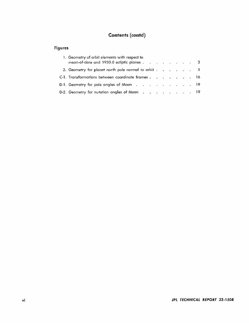
1 . Geometry of orbit elements with respect to mean-of-date and 1950.0 ecliptic planes . . . . . . . .

2 . Geometry for planet north pole normal to orbit . . . . . . 3

5

C.1 . Transformations between coordinate frames . . . . . . . 16

D.1 . Geometry for pole angles of Moon . . . . . . . . . 19

0.2 . Geometry for nutation angles of Moon . . . . . . . . 19

JPL TECHNICAL R E

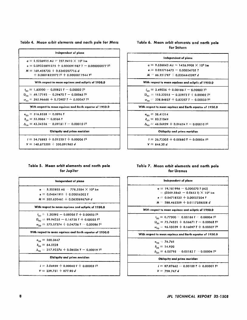
Expressions are presented for the mean orbital elements of the nine planets with respect to the mean equinox and ecliptic of 1950.0. Also, expressions are presented for the right ascension and declination of the north pole of each of the nine planets with respect to the mean equinox and Earth equator of 1950.0. The expressions are polynomials in time T measured in Julian centuries from the epoch January 1.0, 1950 E.T. The expressions are useful for coordinate transformations and approximate planetary ephemerides in astrodynamic computer programs.

vii

In astrodynamic computer programs, the mean orbital elements of the planets and the planet pole vectors are often needed for purposes such as coordinate transformations or generating approximate planet ephemerides. Polynomial expressions for these quantities are given in sources such as Refs. 1 and 2. However, these expressions give the quantities with respect to the mean Earth equator or ecliptic of-date, whereas a common fixed coordinate system is desired for vector operations. For example, in a patched conic interplanetary computer program, the position and velocity of the launch planet at the launch date and the arrival planet at the arrival date would be in different coordinate systems if generated from available mean elements. Thus, coordinate transformations on one or both state vectors are required. A set of mean elements with respect to a common coordinate system would simplify the program logic.

An inertial reference coordinate system currently in wide use is that associated with the mean Earth equator or ecliptic of 1950.0, where the epoch notation refers to the beginning of the Besselian year and corresponds to Julian Ephemeris Date (JED) 2433282.423357. The Jet Propulsion Laboratory (JPL) ephemeris tapes (Ref. 3) and double precision trajectory program (Ref. 4), use coordinates with respect to the mean Earth equator and equinox of 1950.0.

This report presents expressions for the mean orbit elements and pole vectors of the planets and the Sun with respect to the 1950.0 coordinate systems. The derivations are described in detail, and numerical results are given. In addition, some variables useful for coordinate system transformations are given. Coordinate system transformations are discussed in Appendix C. A list of symbols and nomenclature is also provided to define the

1

notations used in the polynomials and coordinate transformations. 1950.0

(2) Tt, , time in tropical centuries from the epoch

to the standard time unit selected for the derived polynomials of this report. The equations also show the coefficients of the desired polynomial in terms of the given polynomial coefficients.

Because of their rapidly varying nature, lunar angles are not suitable for representation as 1950.0 polynomials, but are best handled in terms of the mean-of-date polynomials. Special consideration of the Moon is discussed in Appendix D.

To = T + 0.5

ce its e

When coordinates are specified with respect to some system, two different times are used. The first time is that at which the coordinate reference planes are defined to exist; the second time is that at which the coordinate components are desired. In of -date polynomials, these two times are the same; i.e., the reference plane is defined at the same instant as the coordinate components are evaluated. The reference planes for the polynomials presented in this report are defined at the epoch 1950.0, and remain fixed. Therefore, the time in the polynomials refers only to the time at which the values of the coordinate components are measured.

Time in the polynomials is measured from some reference epoch and in some units. In selecting a reference epoch, one might first choose the epoch 1950.0, since it is also used to define the reference planes. However, this epoch is an awkward number. It has many decimal places when expressed as a Julian date or in conventional days, hours, minutes, and seconds. To avoid this disadvantage, the reference epoch is selected as a nearby even date: 1950, January 1.0, E.T. (JED 2433282.5). Thus, the beginning of any ephemeris day is counted in whole numbers of days from the reference epoch. It is important to remember in the following derivations that the time reference epoch and the coordinate system epoch are not exactly the same instant.

For these applications, it is common in technical literature to find time measured in one of the following units: (1) ephemeris days, (2) Julian centuries, or (3) tropical centuries. Time is also measured from one of the following reference epochs: (1) 1950.0; (2) 1900, Janu- ary 0.5, E.T.; or (3) 1950, January 1.0, E.T.

Equations (1) and (2) define the conversion from the following two common polynomial time units:

(1) To, time in Julian centuries from the epoch 1900, January 0.5, E.T.

A = a, + a, To + a, T t + a,T;

= (a, + 0 . 5 ~ ~ f 0 . 2 5 ~ ~ + 0 . 1 2 5 ~ ~ ) (1) + (a, + a, + 0 . 7 5 ~ ~ ) T

+ (a, + 1.5U3) T2

+ a,T3

where T = time in Julian centuries from the epoch 1950, January 1.0, E.T.

36525.0 0.076643 36524.21988 36524.21988 Tt, =

= F T + k

A = a, + a, T , , + a, T & + a, T;=

= (a, + a,k + azkZ + u3k3)

+ (a$ + 2u, Fk + 3a, Fk2) T

+ (a, F2 + 3a, F2k) T Z

+ (a, F 3 ) T3

it ent

Table 13 of Ref. 2 contains polynomials in T o for mean orbit elements with respect to the mean equinox and ecliptic of-date for all planets except Pluto. These polynomials were developed from sources given in Ref. 1. (The mean anomaly, because of the more rapid variation, may have the linear time term in units of days, &.)

The first step in converting to &e new polynomials is to convert the given expressions according to Eq. (1) to obtain polynomials in T . This step changes the reference epoch from 1900, January 0.5 to 1950, January 1.0. Since the mean anomaly M, the eccentricity e, and the semimajor axis a are independent of coordinate systems, their polynomials are now in the form desired. It remains to

MEAN PLANET ORBIT AT T

< - " 1

/ 1950.0 ECLIPTICA

Fig. 1 . Geometry of orbit elements with respect to mean-of-date and 1950.0 ecliptic planes

transform the other three elements i, 0, and o to the desired coordinate system.

Figure 1 illustrates the geometry of the problem. The spherical triangle Nan50 has the known side r ~ 1 - A and the known angles rl and i. The solution for the unknown sides and angle has the form

sin i 5 0 sin (050 - II,) = sin i sin (a - A)

sin i5, cos (aso - II,) = COS i sin r1

+ sin i cos r1 cos (a - A)

cos i50 = cos i cos rl

- sin i sin r1 COS (a - A)

sin i5, sin

sin i50 cos ("50 - 0) = sin i cos rl

- 0) = sin T, sin (a - A)

+ cos i sin r1 COS (a - A)

(3)

Two methods are used to obtain the desired polynomials for i 5 0 , a 5 0 , and W50 from Eq. (3).

A. Least-Squares Curve-Fit Method

Steps for using the least-squares curve-fit method are

(1) Evaluate the known polynomials for i, a, W, A, II,, and at selected values of T over the time period of interest. The values used are T = 0.0, 0.1, 0.2, 0.3,0.4, and 0.5 for a total of six points.

(2) Compute the right hand sides of Eq. (3) at each value of T.

listed below:

(3)

(4)

Solve Eq. (3) to obtain values of is0, a50, and ws0

at each value of T.

Perform a least-squares curve-fit to the data from step (3). In this step, the elements are assumed to be representable as power series in T to an ap- propriately low order; i.e., 2 or 3. The curve-fit yields the coefficients of the desired polynomials.

In step (l), the known quantities A, w1, and IT1, per- taining to earth precession, are obtained from the Ref. 5 expressions that are given in the tropical century form:

sin r1 sin II, = 4?585765 T, , $. 0!'19435 Tt,

- 0'100022T3tr

sin rl COS II1 = - 46'184975 T,, + 0'10525 T:T

+ (Y'00032 T:r

A - I I l = 5026'17515 T,, + 1'.'1116 c, + 0'100014 T3,,

(4)

In the first two expressions of Eq. (4), the use of seconds- of-arc to represent the product of two trigonometric functions may be confusing. The actuaI numerical value of the product is obtained by converting seconds-of-arc to radians.

In the least-squares curve-fit method, each expression of Eq. (4) is evaluated numerically in the form it appears. In the series manipulation method, which is described in the next subsection, these expressions are converted to direct polynomials in T for the quantities A, TI,, and rl themselves, rather than their trigonometric functions. These converted expressions are actually those desired for the mean elements of Earth, since by definition (for Earth only)

(5)

The results of the least-squares curve-fit method agree very closely with the results of the series manipulation method and are summarized in Section V of this report.

The JPL double precision trajectory program, DPTRAJ (Ref. 4), provides an interesting alternative that is equivalent to the least-squares curve-fit method. The link

JPL TEC 3

TRIC of DPTRAJ provides transformations between various coordinate systems. The link TRIC was used to rotate the elements i, 0, and w (with respect to the mean equinox and ecliptic of-date) to the elements i50, a 5 0 9

and 050 (with respect to the mean equinox and ecliptic of 1950.0). The results were then fit with polynomials as previously mentioned in step (4). The TRIG coordinate transformation uses the Cartesian transformation matrix

= {GO}$ {eo - 90"}, { -e},{90" + Z},{- qz

involving the equatorial precession angles eo, 8, and 2 and the mean obliquity, zi (Refs. 2 and 5). The least-squares curve-fit method, although solving the spherical triangle equations of Eq. (3) directly, is effectively using the Cartesian transformation matrix

which involves the ecliptic precession angles. When the and R are equated, equations result for II,,

T, and A in terms of Z, eo, 8, and 2. The solution of these equations gives a check on the consistency between Eq. (4) and the more commonly used expressions for E, eo, 8, and 2. (See Eqs. 11 and 16.) This subject is explored more fully in Appendix A.

The series expressions used in this method are developed in detail in Appendix B. The numerical results of the series manipulation method agree very closely with the results of the least-squares curve-fit method, and are summarized in Section V.

As stated at the beginning of this section, the elements of Pluto were not obtained by the preceding methods. The values of i50, aso, and 6&0 for Pluto are adopted as constants and are equal to the osculating values from Table 23 of Ref. 2. (Both the values in Ref. 2 and those adopted here are from the JPL ephemeris DE 19, Ref. 3).

e~~vat~on of the

Reference 2 gives expressions for the right ascension and declination of the mean north pole with respect to the mean equinox and equator of-date for the Sun, Venus, Mars, Jupiter, Saturn, Uranus, and Neptune (the mean pole neglects nutation). The expressions are linear in time and are measured from a variety of reference epochs. The rate term accounts for the combined precession of the Earth equator and the planet equator, using expressions derived in Ref. 6. The form of the expressions is

a = atO + & (t - to)

8 = 8to + 8 (t - to)

Steps for using the series manipulation method are where I5 and b are evaluated by the terms of Eq. (7) at the reference epoch to listed below:

(1) Consider the known polynomials for i, 0, W, A, 111,

small increment. Expand the sines and cosines of the polynomials as power series in the small increment.

& = m + n s i n a tan8 +psinIcosAsec8

6 = ncosa+ps inIs inA and Tl to have the form of a leading term plus a (7)

The h s t term in Eq. (7) accounts for the precession of the Earth and the second term accounts for the precession of the planet. To get a50 and 850 (with respect to the mean equinox and equator of 1950.0), perform the following steps:

(2) Perform series multiplications, additions, and divi- sions indicated in Eq. (3) to obtain series expressions for the tangents of iso, n50 - II,, and 0 5 0 - 0.

(3) Expand the arc tangents as power series in a small (1) Substitute t = 1950.0 in Eq. (6) to obtain as0 and increment. 8 5 0 at the epoch 1950.0.

(4) Make final series additions to yield the desired (2) Evaluate the rates using only the second term of polynomials for is0, a 5 0 , and os@. Eq. (7):

Preparatory to step (I), the expressions of Eq. (4) are converted by similar series manipulations to obtain the starting polynomials in II,, r1, and A.

&50 = p sin I cos As0 sec 8,,

850 = p sin I sin A50 (8)

(3) The planet precession rate p is commonly available as a rate per tropical century. Therefore, steps (1) and (2) give expressions that can be transformed by Eq. (2) to the desired form

MEAN PLANET

Earth, Mercury, and Pluto require special treatment, separate from that for the other planets and the Sun. For

directly, since by definition

1950.0 MEAN Earth, the precession angles yield the desired forms EARTH EQUATOR

Fig. 2. Geometry for planet north pole normal to orbit

a50 = -&I

8 5 0 = 90" - 0 (lo) Eq. (2). For use in Eq. (lo), first transform Eq. (11) according to

References 2 and 5 give the following: North pole vectors have not been determined for Mercury and Pluto; however, the common assumption will be made that the pole is normal to the orbit. The geometry for this is shown in Fig. 2. Solving the spherical triangle y 5 0 N a in the same manner for Eq. (3) gives

to = 2304!'9516 Tt, + 0!'3022 T:, + W0180 T: ,

6 = 2004Y2573 Tt, - 0'!4268 T i , - 0!'0418 T:,

sin (90" - 850) sin (a5, + 90") = sin i50 sin a 5 0

sin (90" - S,,) cos (a50 + 90") = cos i50 sin Zs0 + sin i,, cos Zs0 cos a5,

cos (90" - 850) = cos i,, cos Go - sin i50 sin Z5,, cos

sin (90" - 850) sin A 5 0 = sin P,, sin a250

sin (900 - 850) cos = sin i50 cos z~~ + cos i,o sin z~~ cos as0 I

Equations (12) are evaluated for Mercury and Pluto, and the numerical results are given in Section V. For Pluto, the pole vector is fixed because the orbit elements are constant, but for Mercury, the rates on aSO and S,, are those required to keep the pole normal to the changing orbit. These rates cannot be related to a Mercury precession, as in Eq. (8), since the obliquity I is zero.

The specification of a planetary orbit and equator allows the defmition of a planet vernal equinox in a manner analogous to that for Earth; i.e., the ascending

node of the orbit on the equator. The planet equinox is used as a reference direction in planetary coordinate systems. The angle along the planet equator, measured from the ascending node on the mean 1950.0 Earth equator to the autumnal equinox a50 is useful in coordinate transformations. Another useful angle is that between the orbit and equator of the planet; i.e., the planet obliquity I . The solutions for A50 and I are obtained from spherical triangles and appear in Ref. 1 (p. 332). They are reproduced here with subscript 50 to denote the use of the mean 1950.0 ecliptic and equator, rather than the mean-of-dute in the Ref. 1 equations.

5

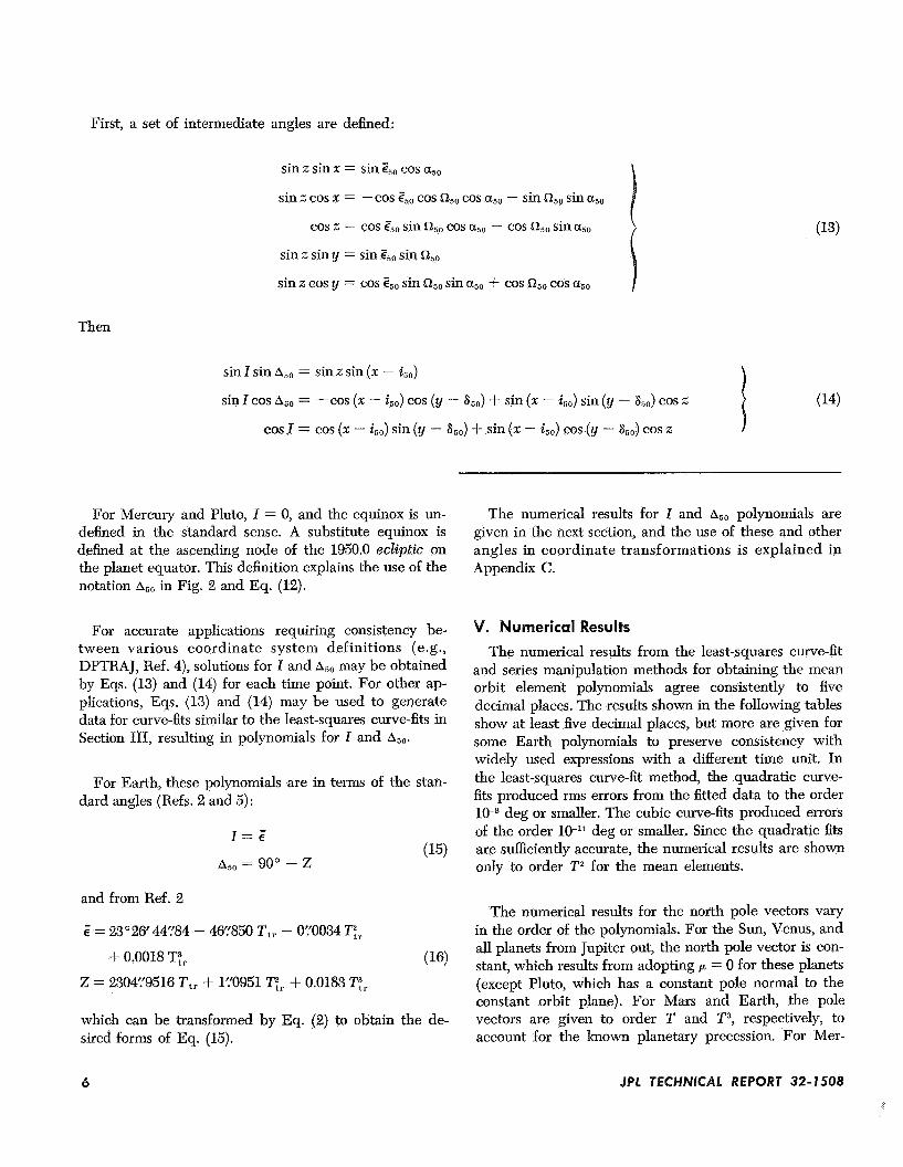
First, a set of intermediate angles are defined:

sin z sin x = sin 250 cos a50

sin z cos x = -cos g50 cos as0 cos a50 - sin a 5 0 sin a50

cos z = cos %0 sin a50 cos as0 - cos 05" sin a50

sin z sin y = sin g50 sin Kt50

sin z cos y = cos 250 sin a 5 0 sin a50 + cos a 5 0 cos asO

Then

sin I sin Aso = sin z sin (x - iso)

Sin I cos AtiO = -cos (x - i 5 0 ) cos (y - 8 5 0 ) + sin (x - i50) sin (y - as0) cos x

cos I = cos (x - i 5 0 ) sin (y - a5J + sin (x - i 5 0 ) cos (y - a5,,) cos z

For Mercury and Pluto, I = 0, and the equinox is un- defined in the standard sense. A substitute equinox is defined at the ascending node of the 1950.0 ecliptic on the planet equator. This definition explains the use of the notation A50 in Fig. 2 and Eq. (12).

The numerical results for I and A50 polynomials are given in the next section, and the use of these and other angles in coordinate transformations is explained in Appendix C.

For accurate applications requiring consistency between various coordinate system definitions (e.g., DPTRAJ, Ref. 4), solutions for I and A50 may be obtained by Eqs. (13) and (14) for each time point. For other applications, Eqs. (13) and (14) may be used to generate data for curve-fits similar to the least-squares curve-fits in Section 111, resulting in polynomials for I and Aso.

For Earth, these polynomials are in terms of the standard angles (Refs. 2 and 5):

w~erical Results

The numerical results from the least-squares curve-fit and series manipulation methods for obtaining the mean orbit element polynomials agree consistently to five decimal places. The results shown in the following tables show at least five decimal places, but more are given for some Earth polynomials to preserve consistency with widely used expressions with a different time unit. In the least-squares curve-fit method, the quadratic curve- fits produced rms errors from the fitted data to the order

deg or smaller. The cubic curve-fits produced errors of the order lell deg or smaller. Since the quadratic fits are sufficiently accurate, the numerical results are shown only to order T2 for the mean elements.

and from Ref. 2

E = 23 26' 44'184 - 46'1850 T t - 0'.'0034 T2,, The numerical results for the north pole vectors vary

in the order of the polynomials. For the Sun, Venus, and all planets from Jupiter out, the north pole vector is constant, which results from adopting p = 0 for these planets (except Pluto, which has a constant pole normal to the constant orbit plane). For Mars and Earth, the pole vectors are given to order T and T3, respectively, to account for the known planetary precession. For Mer-

(16) + 0.0018 T:,

Z = 2304'.'9516 T,, + 1'10951 T , + 0.0183 T;,

which can be transformed by Eq. (2) to obtain the desired forms of Eq. (15).

6 JPL r E C H ~ l C A L R E P Q ~ r 32-1508

cury, the pole vector is given as a curve-fit to order T 2 to keep the pole normal to the changing orbit plane.

Additional angles useful for coordinate transformations are I, and V. Curve-fits to computed values of I and A ~ , , are listed in Tables 1-10. The right ascension of the prime meridian V (also known as the hour angle of the equinox) is derived as outlined in Ref. 1 (p. 336).

The convention of measuring longitude positive East, which is opposite to that in Ref. 1, is used by JPL. There- fore, in JPL convention, the signs are reversed in the expression for the longitude of the central meridian LCM. The JPL expression is

For more detail, see Ref. 7.

For the Sun, Venus, Earth, Mars, and Jupiter, expressions from Ref. 2 are converted to the standard time unit d, which is measured from January 1.0, 1950 E.T. For Mercury, zero longitude is defined as that through the subsolar point at the perihelion on May 1, 1968 (JED 2439978.30246).

For Saturn, Uranus, Neptune, and Pluto, V is adopted as zero on the reference epoch January 1.0, 1950 E.T.

Table 1 . Mean orbit elements and north pole for Mercury

.000000030 T2

= 280.86554 - 0.03289 T - 0.00001 T2

6,, = 61.39767 - 0.00471 T -!- 0.00001 T2

V = 343.54720 -k 6.136 d

I = 176.52462 - 0.01

V = 3 17.695584 + 1.4

Table 3. Mean orbit elements and north pole for Earth

e = 0.0167301085 - 0.000041926T - 0.000000126T2

M = 358.000682 + 0.9856002628d -0.0001550000 T2 - 0.0000033333 T3

With respect to mean equinox and ecliptic of 1950.0

i,, = 0.01 3076 r - o.ooo009 TZ

05, = 174.40956 - 0.241 66 T + 0.00006 T2

w6, = 287.67097 + 0.56494 T + 0.00009 T2

With respect to mean equinox and Earth equator of 1950.0

as0 = - 0.0000013435 -0.6402780091 T

a,, F 89.9999988317 - 0.5567500297T

Aso = 89.9999986565 - 0.6402780100 T

- 0.0000839481 T2 - 0.50003 X lO-5T3

-!- 0.0001 185607 T2 d- 0.00001 161 19 T3

-0.0003042075 T2 - 0.0000050837 T3

Obliquity and prime meridiana

I = 23.4457888616 - 0.0130141669 r - 0.09445 x 10-5 ~2 + 0.050oo x 10-5 r 3

E.T. - (1.002737909294 + 0.589 X loblo T) (E.T. - UT1)

240 V =

-!- 100.0755426042 -k 36000.76931 20833 T + 0.0003870833 rz

aE.T. and UTI are expressed in seconds from zero hours on current day.

7

a = 1.5236915 AU = 227.9410 X lo6 km

e = 0.09335891 275 + 0.000091987 T - 0.000000077 T2

M = 169.458720 + 0.5240207716 d

With respect to mean equinox and ecliptic of 1950.0

i,, = 1.85000 - 0.00821 T - 0.00002 T2

a,, = 49.171 93 - 0.29470 T - 0.00065 r2


u5, = 316.8538 - 0.0996 T

6,, = 53.0066 - 0.0566 T

= 43.34526 - 0.09181 T - o.oooio r2

I = 24.76883 + 0.01 220 T -k 0.00006 T2

V = 148.672501 -k 350.891962 d

Table 5. Mean orbit elements and north pole for ~upi ter

Independent of plane I a = 5.202803 AU = 778.3284 X lo6 km

e = 0.0484191 1 + 0.00016302 T

M = 302.650461 -k 0.0830898769 d

With respect to mean equinox and ecliptic of 1950.0 I i,, = 1.30592 - 0.00205 T 4- 0.00003 T2

a,, = 99.94335 - 0.1 6728 T + 0.00055 r2

w5, = 273.57374 + 0.04756 T - 0.00086 TZ


a,, = 268.0447

a,, = 64.5528

A5, = 317.92374 -k 0.08006 7' - 0.00019 T2

a = 9.538843 AU = 1426.9908 X lo6 km

, = 1 i3.22015 - 0.25973 r + 0.00002 r2

a,, = 38.41314

a,, 83.31049

A5,, = 46.06929 d- 0.01 624 T - 0.0001 0 T2

I = 26.73305 + 0.00880 T

Table 7. Mean orbit elements and north pole for Uranus

Independent of plane

a 19.1 8 1996 - 0.000570 T (AU) = (2869.5862 - 0.0853 TJ X lo6 km

e = 0.0471 8232 f 0.00027204 T

M = 288.465359 -k 0.01 17258558 d

i,, = 0.77300 - 0.001 86 T - 0.00004 T2 Os, = 73.74521 -f- 0.06671 T - 0.00068 T2

w50 = 96.10329 + 0.16097 r + o.00037 r2

I With respect to mean equinox and Earth equator of 1950.0 I as, = 76.761 a,, = 14.920

Obliquity and prime meridian

I = 97.97862 - o.ooioo r + o.ooooi 1 2

V = 798.767d

8 J 32- I508

= (4496.5623 -!- 0.181OT) X l o 6 t m

Q,, = 13 1.22959 - 0.00574 T - 0.00029 T2

a,,, = 295.5712

a,, = 41.46635

= 17.21 185 - 0.00078 T - 0.00002 TZ

I = 28.80226 - 0.00016 T - 0.00001 T2

V = 617.143 d

Independent of plane

a = 39.3736414 AU = 5890.2138 X lo6 km

e = 0.2488033

M = 301.68757 -I- 0.0039892964 d

With respect io mean equinox and ecliptic of 1950.0

i,, = 17.16987

a,,, = 109.68346


a,, = 313.89136

a,,, = 66.36420

A,, = 69.13587

I = 0.0

V = 56.338 d

Table IO. Mean orbit elements and north pole for Sun

J P L TE 9

From planetary theory and the adopted values of the precession constants (see Ref. 5), expressions for the mo- tion of the ecliptic are obtained that are reproduced in this report as Eq. (4). Additional expressions for the equatorial precession angles and the mean obliquity are also obtained; these are shown in Eqs. (11) and (16). The latter expressions for to, e, Z, and Z are widely published (e.g., Refs. 1, 2, and 5) and used in computer programs to perform coordinate transformations.

The coordinate transformation from mean equinox and ecliptic of-date to ecliptic of 1950.0 may be done in terms of the commonly available equatorial precession angles by the matrix

= {&O}S {to - goo}, { -e}, {goo + z } ~ { -">,

Alternately, this transformation may be done more directly in terms of the ecliptic angles by the matrix

(A-1)

When matrices Q and R are equated, equations are produced that give n,, rl, and A as functions of to, 9, Z, and t.

(1,3)l

(2,3) -sin r1 COS n, = - COS cS0 COS co COS z sin + cos 250 sin to cos 6 sin z sin - cos &, sin 5, sin 6 cos

sin rl sin Etl = - sin to cos Z sin 5 - cos to cos 6 sin Z sin ii + cos to sin e cos 5

+ sin E,, sin e sin Z sin E + sin E50 cos e cos E

(3>3) cos r1 = sin Go cos 5, cos Z sin 7 - sin z50 sin 5, cos e sin Z sin Z + sin E5, sin to sin e cos E + cos E5, sin e sin Z sin E + cos &-,, cos e cos E

( 3,l)

(3,2)

-sin rl sin A = sin E50 cos to sin Z + sin E5,, sin lo cos 9 cos Z - cos E,, sin 9 cos Z

sin rl cos A = - sin Go cos 5, cos Z cos E + sin Z550 sin to cos e sin Z cos E + sin &,, sin to sin e sin E - cos ESo sin e sin Z cos Z + cos Z5, cos e sin E

(A-3)

When the adopted values of to, 8, Z, and Z are substituted from Eqs. (11) and (16) into Eq. (A-3), the results are the values for rl, n, and A that are listed in Table A-1. If these values are compared with values computed directly from Eq. (4), there are disagreements of as much as 0.00009 deg.

However, the more fundamental quantities are rl, Ill, and A. A reverse solution can be obtained by equating the two matrices

* = { t o - go"}, { - e } , {goo + Z}, ( A-4)

'Numbers in parentheses refer to the row and column, respectively, of the expanded Q and

10 JPL T E C H ~ / C ~ L REPORT 32-1508

-4. les

174.52504 1 74.361 17

0.2561 26 0.320162

The results give lo, e, and Z as functions of r,, XI,, A, and E .

(2,3) -sin e sin lo = sin Z {cos €50 [sin II, sin A + cos II, cos rl cos A] - sin E;, sin T, cos A}

+ cos Z { -cos $,, cos Ill sin r, - sin z50 cos T ] }

sin e cos lo = sin Z {cos 11, sin A - sin 11, cos r1 cos A} + cos (1,3) sin Ill sin zl

cos e = sin Z {sin Z5, [sin n, sin A + cos II, cos rl cos A] + cos Zs0 sin rl cos A} 64-5)

(3>3)

f cos Z { - sin G O cos II, sin rl + cos z50 cos rl}

(3,2) - sin 6 sin Z = cos Z {sin Go [sin 111 sin A + cos II, cos r, cos A] + cos z 5 0 sin T, cos A}

+ sin E {sin z 5 0 cos II, sin r, - cos E;, cos r,}

(3,l) - sin 0 sin 2 = sin $0 [sin II, cos A - cos 111 cos rl sin A] - cos Go sin r, sin A

Substitution of the adopted values of r,, II,, A, and E from Eqs. (3) and (16) into Eq. (A-5) gives the values for lo, e, and 2 that are listed in Table A-1. If these values are compared with adopted values from Eqs. (11) and (16), there are disagreements of up to O.ooo008 deg.

These inconsistencies are sometimes troublesome in high-precision computations. For most users, however, the small differences can be neglected.

It is not clear to what extent the differences in Table A-1 are due to numerical errors in performing the computations in Eqs. (A-3) and (A-5). The values in Table A-1 are rounded from values computed in double precision on the Univac 1108, producing 18 figures. Not alI 18 figures may be significant, however, because of small differences of nearly equal quantities.

JPL T ~ C ~ ~ I ~ A L REPORT 32- 7 508 11

When consistency is a necessity for the Earth angles, the procedure used in Section IV for the other planets can also be used for the Earth. To review, the steps of this procedure are as follows:

(2) Noting the equivalences of Eq. (lo), evaluate and 8 5 0 from formulas for the north pole for Earth (Table 3).

(3) Use Eqs. (13) and (14) to compute I and h 5 0 .

(1) Noting the equivalences of Eq. (S), evaluate i50 and G~~ from formulas for the mean orbit elements for Earth (Table 3).

The equivalences of Eq. (15) indicate that the steps listed above provide computed values of Z and 2 as functions of adopted values of &,, IT1, A, rl, to, and 8.

1 JPL r € C ~ ~ / ~ A ~ REPORT 32-1508

S COS a = cos a,

For basic expansions of small angIe x, to the order x3, the following equations are used:

x3

6 sinx= x-- (B-1)

X2

2 cosx= 1 - - (B-2)

x3 3 t anx= x + - 03-31

1. Sine osine Series

Given

a = a, + a1 T + a, T 2 + a, T3

Find

sin a = So + S, T + S, T 2 + S , T3

+ [ -al sin a,] T

1 1 2 -az sin a, - - a ; cos a, T Z

1 1 + [ - ( a3 - 6 a:) sin a, - a, az cos a, T 3

03-5)

ultiplication and Division

Given

A = a, + a, T + a, T2 + a, T3

B = bo + b, T + b, T 2 + b, T3

Find

cos a = C , + C, T + C , TZ + C , T3 C AB = CO + ci T + CZ T2 + C S T3 A B D =- =do + d, T + d,T2 + d, T3 Let

a = a o + x

where x is a small angle:

x = az T + a, T2 + a, T3 Elementary term-by-term algebraic multiplication gives

C = a, bo sin a = sin a, cos x + COS a, sin x cos a = cos a, cos x - sin a, sin x + [a, bo + a, b,l T

Using Eqs. (B-1) and (B-2) and retaining terms of order T3, we determine

sin a = sin a,,

+ [al cos a,] T

1 1 2 a, COS a, - - aZ, sin a. T2

+ [a, bo f a, b, + a, b,] T2

+ [a, bo + a, b, + a, b, + a, b31 T3 (B-6)

Let

1 1 b b2 B bo b, - = - [ 1 + (e T + - T Z +

Expand 1/B by binomial theorem, and by the use of (33-4) (B-6) for A * (l /B)

1 1 + [ ( a3 - -g- a; ) cos a, - a, a, sin a, T3

a3 a,b3 + albz + albl 2a,blbz + a,b; a,b: + - 7 1 T3 b: b: b, 03-7)

13 AL RE~ORT 32-150

Given

tana = to + t , T + tz T 2 + t, T3

Find

a = a. + a, T + a2 T2 + a3 T3

Let

a = a o + x

where x is a small angle:

tan a,, + tan x 1 - tan a,, tan x tan a =

which by Eq. (B-3) becomes

to + (x + ;) 1 - t o (x + ;) tana =

by expansion in powers of x

tan a = to + x (1 + t:) + x2 to (1 + t i)

+ x3 (+ + t i ) (1 + t:)

by substitution for x and expansion

tan a = to + [a , (1 + t i )] T + [a, (1 + ti) + a: to (1 + t:)] T z

Equating of like coefficients of T in Eqs. (B-8) and (B-9) allows the solution for the desired coefficients:

an = tan-' (to)

a1 = - tl 1 + tg

(B-10)

14

S

To facilitate the description of coordinate transformations, it is useful to first state several working definitions. Three characteristics of coordinate systems are used: (1) frame, (2) center, and (3) type. Thus, individual coordinate transformations involve a change in frame, center, or type, and a complete transformation generally involves a series of changes of all three. This report deals only with changes of frame.

subsequently, is nonrotating as coordinates are measured with respect to it. The second way is to regard the time to be the same as that of the coordinate values, and is a rotating frame always aligned of-dute. The distinction has implications regarding the velocity rotations and is discussed in more detail later. In summary, a frame is defined by the specification of the following:

(1) Body.

(2) Reference plane.

A. Frame (3) Reference direction.

A coordinate frame (Table C-1) is defined in terms of an associated set of Cartesian axes: x, y, and Z. The X-y plane is a defined reference plane (e.g., the equator plane)

(4) Epoch.

B. Center and the x-axis is a reference direction (e.g., the equinox). The x-axis is normal to the reference plane in a direction corresponding to some physical quantity; e.g., north. The reference plane is generally associated with some body; however, the origin of the frame need not be centered at that body. Reference planes and directions are commonly defined in terms of 8 time at which they exist physically; however, this time is not necessarily the same as the time associated with the coordinate values,

The center of a coordinate frame may be at the center of any of the nine planets, the Sun, the Moon, or a defined station on the surface of any of these bodies. Translation between body centers is accomplished in mean 1950.0 Cartesian coordinates and translation between a bcdy center and a station is accomplished in body-fixed Cartesian coordinates.

C. Type

The reference coordinate frame in this report is the Earth mean equator and equinox of 1950.0 (referred to

Given a center and coordinate frame, there are several types of coordinates commonly used; they are:

as “mean 1950.0). All other frames are defined as rotations from this frame. (1) Cartesian.

(2) Spherical. A frame may be regarded in two ways in relation to

the time designation. The first way is to regard the time (3) Classical conic orbit elements. - - as defining the epoch at which the frame is defined and, (4) Hyperbolic asymptote.

-1. ~ o o r ~ ~ n a t e frames

Name I x-yplane I x-axis I z-axis

Mean equotor ond equinox Mean equator of body Ascending node of mean orbit on meon Direction of body rotation vector (north) equator (mean equinox)

Mean orbit and equinox Mean orbit of body Mean equinox Direction of orbitol rotation vector

True equotor and equinox True equator of body Ascending node of mean orbit on true North I I equator (true equinox) I Mean orbit ond true equinox

Body fixed True equator of body Prime meridian North

Mean orbit of body True equinox Direction of orbital rotation vector

JPL TEC 15

The type used to transfer between coordinate frames is the standard Cartesian coordinate set: (x, y, z, 2, zj, 2).

There are important exceptions to this transformation, and the following rules apply:

§ (1) In transforming from mean 1950.0 to any of-date

frame, the matrix derivative is Frame transformations are done only in Cartesian co-

ordinates, and are shown schematically in Fig. C-1. To transfer from one frame to another, follow the block dia- gram from the initial frame to the mean 1950.0 block (with T = initial epoch) and then back to the desired block (with T = final epoch).

(a) Nonzero if the final output type is Cartesian or spherical.

(b) Zero if the final output type is classical conic orbit elements or hyperbolic asymptote.

(2) In transforming from mean 1950.0 to any epoch At each step, check to see if the current block is the desired final frame or if the next step should branch to one of the orbit blocks.

frame, the matrix derivative is zero.

(3) In transforming from any frame to mean 1950.0, Figure C-1 shows the position transformation matrix the matrix derivative is

in the direction of the arrow. For example,

(5) Body mean equator = A(Z)so and equinoxof T

(a) Zero if the initial type is classical conic orbit elements or hyperbolic asymptote.

The reverse position transformations are simply the trans- poses of those indicated, since all transformations are orthogonal.

(b) Zero if the initial conditions are relative to an epoch frame.

(c) Nonzero if neither (a) nor (b) is true. The velocity transformations are more complicated. In

general, the velocity transformation involves the time derivatives of the transformation matrix. For example,

These rules are based on the philosophy that classical conic orbit elements and hyperbolic asymptotic types are

nated epochs are nonrotating. It is possible with the noted rules to have input and output coordinates that are seemingly close in terms of the number of sequential transformations, but actually must follow a more elab-

- - related to inertial velocities, and that frames with desig- (i) Body mean equator = A ( ~ ) x I + A(-~) ,o

andequinox of T

7 EARTH MEAN

EQUATOR AND EQUINOX OF 1950.0

I 1 A

BODY MEAN I ) ORBIT AND

- E EQUATOR AND

EQUINOX OFT EQUINOX OF T

BODY MEAN

N L

I I I I

I ORBIT AND TRUE EQUINOX OF T

BODY TRUE EQUATOR AND EQUINOX OFT

I I V

I BODY FIXED AT T I

orate sequence. For example, assume the following data:

(1) Initial coordinates : Sun-centered, Earth mean orbit and equinox of-date Cartesian coordinates.

(2) Final coordinates : Sun-centered, Earth mean orbit and equinox of-date classical conic orbit elements.

This would appear to be simply a change of type only; however, it is necessary to rotate first to mean 1950.0 with nonzero matrix derivatives, then back to Earth mean orbit and equinox of-date Cartesians with zero matrix derivatives (to get inertial Cartesian velocities), and then change to classical conic orbit elements.

L I The key to developing the velocity rotation logic is

-1. ~r~nsfor~a~ions etween ~oordin~~e fra whether inertial velocities are needed and where.

All of the transformations in Fig. C-1 are general for all bodies, and are specified in terms of angles, which have the same name but different values depending on the particular body. Equations for evaluating the angles for each body are given in Section V; each matrix remains to be defined in terms of the angles.

Each matrix is developed in terms of individual rotations about the current x-, y-, or z-axis. The notations are defined in the Nomenclature.

A = + 180°}, (90' - S,,}, {aso + 90°},

N = ET L E = {-E}, { - 8 q},

The nutation angles (8$, 8 ~ ) are not specified in this report. Actually, the nutation is unknown for all bodies except the Earth and the Moon, and therefore 8$ and 8e are adopted as zero. For Earth, expressions are given in Ref. 1 and are also tabulated on the JPL ephemeris tapes (Ref, 3). Special consideration for the Moon is discussed in Appendix D.

JPL T € C ~ N I C A L REPORT 32-7508 17

The angles of the Moon are rapidly varying and cannot (2) be represented with respect to the 1950.0 system by polynomials of low order in T. To obtain the 1950.0 angles for use in standardized coordinate transformation matrices, such as those in Appendix C, the following steps are recommended:

(3)

(1) Evaluation of mean-of-date polynominals for mean orbit elements. These polynomials are found from expressions in Ref. 1 (p. 107). Converting by Eq. (l), we obtain, with respect to the mean equinox and ecliptic of T

Computation of i so , Ow, and w50 for the Moon. This computation is accomplished in the same manner as for the planets in the least-squares curve-fit method of Section 111, by the use of Eq. (3).

Mean obliquity for the Moon. This is the sum of i in step (1) and 1', the constant angle between the ecliptic and the mean lunar equator (see Eq. 79, p. 26, Ref. 2).

I' = 1.533611

I = i + I' = 6.679007 03-3)

i = 2 sin-l( y ) = 5.145396

O = 12.112791 - 1934.139929 T + 0.002081 T2 + 0.000002 TJ

, , ,=r ' -~ = 196.731198 + 6003.163629 T - 0.012425 T2 - 0.000014 T 3

and independent of plane

u = 384399.3 km (uc in Table 17 of Ref. 2)

e = 0.05490 0489

M = c - r ' = 215.531463 + 477198.858310 T + 0.009214 T 2 + 0.000014 T 3

This equation comes from Cassini's second and third laws of the lunar rotation (see p. 27, Ref. 8).

(4) Computation of a50, S50, and As0 for the Moon. The geometry of this problem is shown in Fig. D-1. First, the spherical triangle fi Q E is solved for the intermediate angle p, and sides x and y

(D-1)

O* = O - A + 180" 03-41

sin p sin x = sin T, sin a*

sin p cos x = cos T, sin I' + sin T, cos I' cos a*

cos p = cos T, cos I' - sin T, sin I' cos a* (D-2)

sin p sin y = sin I' sin O*

sin p cos y = sin T, cos I' + cos T, sin I' cos O*

Next, the spherical triangle y 5 0 N Q is solved for the desired angles

sin (90" - 8 5 0 ) sin (A50 - x) = sin z 5 0 sin (II, + y)

sin (90" - a,,) cos - x) = cos sin p + sin E50 cos p cos (E, + y)

cos (90" - 8 5 0 ) = cos E50 cos p - sin 250 sin p cos (II, + y)

sin (90" - S s 0 ) sin (aso + 90") = sinp sin (II, + y)

sin (90" - S s 0 ) cos (a50 + goo) = sin E50 cos ,B + cos E50 sinp cos (II, + y)

1% JP6 T ~ C ~ ~ l C ~ ~ REPORT 32-1508

MEAN LUNAR EQUATOR OF T

MOON MEAN AUTUMNAL EQUINOX

/ Fig. D-1. Geometry for pole angles of Moon

Computation of Moon nutation angles. The nuta- tions of the Moon are commonly represented by the physical libration angles T, U, p. The equivalent Moon nutation angles, analogous to those used for the Earth, are shown in Fig. D-2. First, evaluate the physical libration angles as specified, for example, in Ref. 2 (p. 26). Then, solve the spherical triangle YaNYa in Fig. D-2 (Ea = I from Step 3).

sin Ea sin ( - Sqa) = sin (I’ + p) sin u

sin Ea COS (- Sqa) = COS (I’ + p ) sin i

+ sin (I’ + p ) cos i cos u

COS Ea = COS (I’ + p ) COS i - sin (I’ + p) sin i cos u

sin Ea sin X* = sin i sin u

sin ea COS X” = sin (I’ + p) cos i

+ cos (I’ + p) sin i cos u

(a) EARTH NUTATION ECLIPTIC

/ OF-DATE

, . . .- - -. .. . . . . EQUATOR OF-DATE

(b) MOON NUTATION

L f l + ~ - R - LT +180°

Fig. D-2. Geometry for nutation angles of Moon

(6)

Steps those

Computation of hour angle of true equinox. The hour angle of the true equinox is (from Fig. D-2)

1-6 provide a set of Moon angles equivalent to in Section V for use in the coordinate transfor-

mations of Appendix C .

JPL r E C H ~ ~ C A 1 REPORT 32-7 508 19

A

a09 01, a,, a3

a

A, d

do E

- E

E.T.

e

F

I‘

I i

JED k

L

LCM

M

m

N

n

coordinate transformation matrix (see T time in Julian centuries from January Fig. C-1) 1.0, 1950

general polynomial variable

general polynomial coefficients

semimajor axis

planetocentric right ascension of Earth

ephemeris days from January 1.0, 1950

ephemeris days from January 0.5, 1900

coordinate transformation matrix (see Fig. C-1)

coordinate transformation matrix (see Fig. 6-1)

ephemeris time

eccentricity

ratio of Julian to tropical century (see

angle between ecliptic and mean lunar equator of-date

general mean obliquity for all planets

inclination of mean orbit to ecliptic

Julian Ephemeris Date

tropical centuries from 1950.0 to Janu- ary 1.0, 1950 (see Eq. 2)


longitude of central meridian

mean anomaly

general precession in right ascension


general precession in declination

coordinate transformation matrix (see Section 111)

coordinate transformation matrix (see Section 111)

Eq. 2)

T Earth-planet distance at epoch defining LCM

To

T,,

time in Julian centuries from January 0.5, 1900

time in tropical centuries from 1950.0


hour angle of mean equinox from prime meridian

intermediate angles (see Eq. 13)

Cartesian position coordinates

Cartesian velocity coordinates

angle from true lunar equinox along true lunar equator to descending node on ecliptic (see Fig. D-2)

2 Earth equatorial precession angle (see Refs. 1, 2, and 5) right ascension of planet mean north pole

V

x,y,x

.F = (X,ZJ,Z)~

X = (iyj,2)T x*

-

a

& linear rate of a

p I?’

y

intermediate angle (see Fig. D-1)

mean longitude of lunar perigee

constant of lunar inclination (see Eq. D-1)

angle from node on Earth equator along planet equator to autumnal equinox

declination of planet mean north pole

A

6

i linear rate of s S+ nutation in longitude (Earth)

S E nutation in obliquity (Earth)

S+a Moon nutation in longitude

8% Moon nutation in obliquity

Z Earth mean obliquity

Zc Moon mean obliquity

E Earth true obliquity

Ea Moon true obliquity

[,, Earth equatorial precession angle (see Refs. 1, 2, and 5)

20

e

A

P

Z l

n1

p,%T

T

0

n*

0

w

0

1950.0

Y

Y -

Earth equatorial precession angle (see Refs. 1, 2, and 5)

ecliptic precession angle (see Fig. 1)

planet precession rate (see Eq. 8)



lunar physical libration angles

light time for unit distance in definition of LCM (Eq. 17)

longitude of node of mean orbit on ecliptic

n - A -I- 180" (for use in Eq. D-5)

planet rotation rate in definition of LCM

argument of perihelion of mean orbit

longitude of perihelion = n + 0

beginning of Besselian year 1950 (JED 2433282.423357)

true vernal equinox

mean vernal equinox

mean longitude of Moon

(Eq. 17)

Subscript

50 (1) with respect to the mean Earth equator (or ecliptic) and equinox of 1950.0 when used with variables 7, i, oy w,

6, a, and A

(2) evaluated at the epoch 1950.0 when used with variables ;i, 6, and 4

Rotation matrices

{e}i positive rotation about i-axis by an angu- lar amount e

L o -sin 0

COS e 0 -sin 0

COS e

0 1

sin 0 0

0

sin 9

COS e

{@}I/ =

0

~ ~ I C ~ ~ REPORT 32- 7 508 21

1. Explanatory Supplement to the Ephemeris, Her Majesty’s Stationery Office, London, 1961.

2. Melbourne, W. G., et al., Constaats and Related Information for Astrodynumic Calculations, 1x8, Technical Report 32-1306. Jet Propulsion Laboratory, Pasa- dena, Calif., July 15, 1968.

3. Devine, C. J., JPL Development Ephemeris Number 19, Technical Report 32-1181. Jet Propulsion Laboratory, Pasadena, Calif., Nov. 15, 1967.

4. Khatib, A. R., “Double-Precision Trajectory Program: DPTRAJ,” in Support- ing Research and Advanced Development, Space Programs Summary 37-49, Vol. 11. Jet Propulsion Laboratory, Pasadena, Calif., Jan. 31, 1968.

5. Lieske, J., Expressions for the Precession Quantities and Their Partial Deriva- tives, Technical Report 32-1044. Jet Propulsion Laboratory, Pasadena, Calif., June 15, 1967.

6. De Vaucouleurs, G., “The Physical Ephemeris of Mars,” Icams, Vol. 3, 1964.

7. Sturms, F. M., Jr., “A Proposed Venus Coordinate System,” in Supporting Research and Advanced Development, Space Programs Summary 37-51, Vol. 111. Jet Propulsion Laboratory, Pasadena, Calif., June 30, 1968.

8. Physics and Astronomy of the Moon. Edited by Z. Kopal. Academic Press, New York, 1962.

22 JPL TECHNICAL REPORT 32-1508 NASA - JPL - Coml., L.A., Calif.

TECHNICAL REPORT'STANDARD TITLE PAGE

9 . Performing Organization Name and Address

JET PROPULSION LABORATORY California Institute of Technology 4800 Oak Grove Drive Pasadena, California 91103

12. Sponsoring Agency Name and Address

NATIONAL AERONAUTICS AND SPACE ADMINISTRATION Washington, D.C. 20546

IO, Work Unit No.

Technical Report

15. Supplementary Notes

16. Abstract

Expressions a re presented f o r the mean orbi ta l elements of the nine planets with respect t o the man equinox and ec l ip t ic of 1950.0. Also, expressions axe presented fo r the r ight ascension and declination of the north pole of each of the n h e planets with respect la the mean equinox and Barth equator of 1950,0, centuries from the epoch January 1,0, 1950 E.Ta The expressions are useful fo r coordinate transformations and approximate planetary ephemerides in as t ro

The expressions are polynomials In time T measured in Julia

Unclassified Unclassified

TO FILL OUT THE TECHNIC L REPORT STANDARD TITLE PAGE

Make items 1, 4, 5, 9, 12, and 13 agree with the corresponding information on the report cover. blank. Complete the remaining items as follows:

Use al l capital letters for t i t le (item 4). leave items 2, '6, and 14

3. Recipient's Catalog No. Reserved for use by report recipients.

7. Author(s). lnclude corresponding information from the report cover. In addition, l i s t the affiliation of an author i f i t differs from that of the performing organization.

8. Performing Organization Report No. Insert i f performing organization wishes to assign this number.

10. Work Unit No. Use the agency-wide code (for example, 923-50-10-06-72), which uniquely identifies the work unit under which the work was authorized. Non-NASA performing organizations wil l leave this blank.

1 I. Insert the number of the contract or grant under which the report was

15. Supplementary Notes,

prepared.

Enter information not included elsewhere but useful, such as: Prepared in cooperation with.. . Translation of (or by). * . Presented at conference of.. ~ To be published in.. e

Include a brief (not to exceed 200 words) factual summary of the most significant information contained in the report. I f possible, the abstract of a classified report should be unclassified. I f the repmt contains a significant bibliography or literature survey, mention i t here.

16. Abstract.

17. Key Words. Insert terms or short phrases selected by the author that identify the principal subjects 6o;ered i n the report, and that are sufficiently specific and precise to be used for cataloging.

18. Distribution Statement. Enter one of the authorized statements used to denote releasability to the public or a limitation on dissemination for reasons other than security of defense information. Authorized statements

-are "Unclassified-Unlimited, I' "U. S. Government and Contractors only, 'I

"U. S. Government Agencies only, 'I and "NASA and NASA Contractors only. 'I

19. Security Classification (of report). NOTE: Reports carrying a security classification wi l l require additional markings giving security and dowv- grading information as specified by the Security Requirements Check1 i s t and the DoD Industrial Security Manual (DoD 5220.22-M).

used in preparing announcements, bib1 iographies, and data banks, i t should be unclassified i f possible. rately the classification of the t i t le and the abstract by following these items with either "(U)" for unclassified, or 'f(C)'r or g'(S)l' as applicable for c I assi fi ed i tems.

20. Security Classification (of this page). NOTE: Because this page may be

I f a classification i s required, indicate sepa-

21. No. of Pages.

22. Price.

Insert the number of pages.

Insert the price set by the Clearinghouse for Federal Scientific and Technical Information or the Government Printing Office, i f known.

Documents

With Respect to the - NASA · elements of the planets and the planet pole vectors are ... coordinates with respect to the mean Earth equator and equinox of 1950.0