Wireless Routing

Philip LevisFaculty Lunch, 2/16/10

?

Problem: deliver a packet to a destination across a multihop wireless networkGoal: minimize cost (transmissions/delivery), maximize throughput,

Caveat: commodity wireless in unlicensed bands (802.11, 802.15.4, etc.)

Wireless Routing Today

• Each node sends periodic (15s) beacons

• Measures packet reception ratio (PRR)

• Sliding 20 packet window (5m)

• Compute costs of edges using PRR

• Use standard min-cost graph algorithms

courtesy of Meraki.com

Free the Net, San Francisco

Purple tabs are wired gateways; green nodes provide multihop accessNumbers are hopcount from closest gatewayLines show links

Talk

• What do wireless links really look like?

• 4-bit link estimation

• Datapath validation

• Adaptive beaconing

• powernet.stanford.edu

A Single Transmitter

A Real Network: SWAN

Gates Packard

The Stanford Wireless Access Network (SWAN) is an 802.11b/g testbed at Stanford. It is part of a research collaboration with King Abdullah University of Science and Technology (KAUST).

SWAN consists of 40 custom wireless access points with dual 802.11 radios as well as 10 shuttle PCs for more computationally intensive protocols.

This video shows the packet delivery ratios between the 40 access points over a 2.5 second period. Because collisions preclude measuring all links concurrently, this video is actually 40 temporally consecutive experiments overlaid as being concurrent. These measurements are at 5.5Mbps.

While some links are stable, many are highly dynamic over very short time scales. In particular, the handful of links that bridge Gates and Packard show behavior similar to the stylized example earlier in the talk.

The first step towards overcoming these dynamics is effectively measuring and characterizing them.

A Real Network: SWAN

Gates Packard

The Stanford Wireless Access Network (SWAN) is an 802.11b/g testbed at Stanford. It is part of a research collaboration with King Abdullah University of Science and Technology (KAUST).

SWAN consists of 40 custom wireless access points with dual 802.11 radios as well as 10 shuttle PCs for more computationally intensive protocols.

This video shows the packet delivery ratios between the 40 access points over a 2.5 second period. Because collisions preclude measuring all links concurrently, this video is actually 40 temporally consecutive experiments overlaid as being concurrent. These measurements are at 5.5Mbps.

While some links are stable, many are highly dynamic over very short time scales. In particular, the handful of links that bridge Gates and Packard show behavior similar to the stylized example earlier in the talk.

The first step towards overcoming these dynamics is effectively measuring and characterizing them.

Short-term Link Behavior (burstiness)Conditional Packet Delivery Function (CPDF)

Failures Successes

-100 -50 0 50 100Consecutive failures/successes

0

0.2

0.4

0.6

0.8

1.0

Condit

ional pro

babili

ty

Real Independentβ = 0

Ideal Bursty (I)β = 1.0

-100 -50 0 50 100Consecutive failures/successes

0

0.2

0.4

0.6

0.8

1.0

Condit

ional pro

babili

ty

KW(I) - KW(E)KW(I)

β =

KW(x): Kantorovich-Wasserstein distance of CPDF of x from ideal bursty link B

E: empirical (real) link, I: ideal independent link

-100 -50 0 50 100Consecutive failures/successes

0

0.2

0.4

0.6

0.8

1.0

Condit

ional pro

babili

ty

Real Burstyβ = 0.8

-10 -5 0 5 10Consecutive failures/successes

0

0.2

0.4

0.6

0.8

1.0

Condit

ional pro

babili

ty

Real Oscillatingβ = -0.36

As the interval between packets increases,the distribution of β values moves closer toβ=0. Space packets out far enough and they appear to be independent random trials. Retransmitting a failed packet immediately plays against the odds. Wait long enough and there’s a much less biased coin.

Examining a half dozen or so 2.4GHz networks, we’ve found that 500ms typically is at knee of the beta distribution curve.

β = 1: bursty, β = 0: independent,β = -1: oscillating

Long-term Link Behavior (scaling)

802.15.4 in Gates 802.11b in Free the Net

Networks in the 2.4GHz band observe behavior consistent with scaling: there is no characteristic burst length. The plots above show two links over a thousand-fold difference in time scale. Bursts exist at all time scales.

Discrete wavelet transforms are a standard approach to detect scaling. We construct a logscale diagram (left) of a trace and fit a line with slope α. If α >1, the signal is self-similar (SS); if 0 < α < 1, it is long-range dependent (LRD). Note that the SF link has a dip between octaves 8 and 9, denoting a regular pattern: the cycle of a day.

The plot to the right shows what percentage of links are consistent with scaling in a range of 2.4GHz networks. PRR is packet reception: RSSI is signal strength.

802.15.4 in Gates, α=1.2

802.11b in Free the Net, α=1.12

Controlled (not bursty) link, α=0

Link Estimation (4B)S D

df

drWireless link layers use single-hop acknowledgements. If a node sends a packet and does not hear an ACK, it retransmits. The probability a transmission is considered successful is the product of the two directions. Routing protocols typically measure d through periodic beacons.

ETX = (df x dr)-1

The expected number of transmissions (ETX) can be calculated as the reciprocal of this product. This assumes each packet is a Bernoulli trial.

ETT = min(tb x ETXb)Expected time of transmission (ETT) considers link layers that have multiple bit rates: the ETT is the transmission time at a bitrate (tb) times the ETX at that bitrate (ETXb)

1.5

2

2.5

3

1.5 2 2.5 3

Aver

age

Cos

t (xm

its/p

acke

t)

Average Tree Depth (hops)

White/Compare Bits

Ack Bit: Unidir. Est.

Ack Bit: U

nidir. Est.

Whi

te/C

ompa

re B

its

4BCTP + white bit

CTP + unidirCTP T2

MultiHopLQICost = Depth

45%Directly measuring the datapath leads to more adaptive and accurate link qualities. These benefits can reduce routing costs by 45%.

One problem datapath estimates raise is they only accurately estimate links the protocol uses: this is especially problematic with variable bitrates. This is current work.

1.0Ack Bit ETX

Beacon PRR

Beacon EWMA

Hybrid ETX

1.0 0.83

5.0 3.1 1.72.1

1.25 6

3.9

Received/Acked Packet Lost/Unacked Packet

0.67

1.2

The 4-bit link estimator (4B) directly measures ETX/ETT through the datapath over a 5 packet window. 4B is a hybrid estimator: it merges datapath estimates with beacon estimates.

ETX = α⋅Et-1 + (1-α)Et

Et = 5

ackedconsecutiveunacked{ acked > 0

acked = 0

Taxonomy of Routing Algorithms

Link State Distance Vector

Link CostAB 2AC 2AD 1BD 3BE 1CD 2CF 1CJ 3DE 2DF 4DJ 2EF 2EH 3FG 4FH 2FJ 1

A J

B

E

C

D

F

G

H

1

22

3

1

2

2

4

2

1

2

3

2

1

4

3

A

Neighbor Route LinkA 5 2D 5 2F 2 1J 3 3

C→H:In a link state algorithm, each node has complete knowledge of every link in the network. Each node computes the optimal route to every node in the network using this complete graph.

Whenever a link changes in the network, the protocol must propagate the change to every other node in the network. Once this occurs, every node agrees on the state of the network and routing is consistent.

Generally speaking, link state algorithms converge quickly and are easier to debug, but impose a high communication overhead. This introduces a tradeoff between scale and adaptivity.

In a distance vector algorithm, each node keeps state only on its neighbors. It maintains the cost of links to its neighbors as well as their cost (distance) to each destination. Nodes periodically send control messages to inform neighbors of their costs.

Whenever a link changes the protocol must propagate the change only if it changes distance vectors. For example, suppose DF goes down: D does not need to update any neighbors.

Distance vector algorithms require less state and communication, but the use of limited state leads to many tricky edge conditions, such as persistent routing loops.

B

E

C

D

F

G

H

I3

2

55

22

1

3

A↔H

Distance Vector Challenges and Tradeoffs

S1

S2

D

2

2

10

D: 2

S2: 4

t=0 t=1 t=2 t=4

20 20 20

S1

S2

D2

10

S1: 6

S2: 4S1

S2

D2

10

S1: 6

S2: 8S1

S2

D2

10

S1: 12

D: 10

Distance vector protocols have a tradeoff between agility and overhead. Underlying topology changes can take a number of beacon rounds to resolve: in the above example, when the cost of S2→D changes to 20, it takes several beacon periods to resolve the resulting routing loop. Packets sent into a loop are lost: nodes observe this as a break in connectivity.

The 4B link estimator worsens the problem due to its highly dynamic link estimates. While there are algorithms to avoid the simple example above, there are no known solutions to the general case of preventing all routing loops.

Beaconing faster shortens loop durations and improves packet delivery. But beacons take up valuable link capacity: in low power networks, broadcasts are especially expensive.

1.5

2

2.5

3

1.5 2 2.5 3Av

erag

e C

ost (

xmits

/pac

ket)

Average Tree Depth (hops)

White/Compare Bits

Ack Bit: Unidir. Est.

Ack Bit: U

nidir. Est.

Whi

te/C

ompa

re B

its

4BCTP + white bit

CTP + unidirCTP T2

MultiHopLQICost = Depth

29%

One approach is to only use very good and stable links. Doing so trades off efficiency for stability. MultihopLQI is the highest performance example of this class of approach: it was the dominant protocol before the work in this talk. Routing with the 4B estimator has a 29% lower cost. Using variable links when they are good can reduce transmissions by almost a third.

Datapath Validation

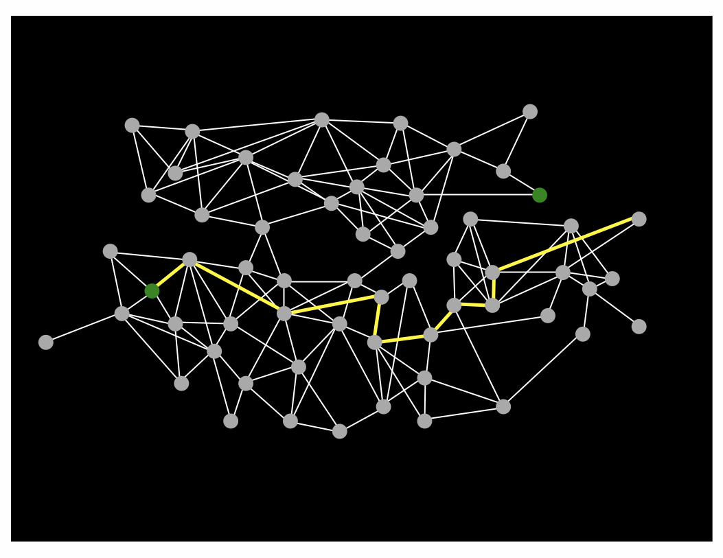
A routing topology is consistent if cost decreases on each hop.

P C ReservedTHLETX

OriginSeq. No.

Data packet header

The routing protocol embeds the transmitter’s ETX cost in every data packet. If a node receives a packet to forward with a lower or equal cost, the topology is considered inconsistent and the protocol triggers a topology repair (more details to follow).

This datapath validation has the additional benefit that it only triggers topology repairs when needed: it couples control packets to the data rate, which is important in low-power networks.

A B C D

01.42.54.1

1.41.11.6

A B C D

03.32.54.1

3.31.11.6

A B C D

03.34.44.1

3.31.11.6

3.3

Consistent

Inconsistent

Mid-repair

0

10

20

30

40

50

60

0 1 2 3 4 5 6 7

Node

id

Time(hours)

This plot shows how common such events are in a sample 60 node testbed. Large network topology changes can cause bursts of correlated routing inconsistencies.

Burst of inconsistencies as topology repairs itself.

Trickle Algorithm

The Trickle algorithm allows nodes in a wireless network to efficiently and quickly reach eventual consistency.

Each node maintains a time window of length τ. When a window expires, it picks a time t in the range of [τ/2, τ) and resets a counter c to 0. When a node hears a “consistent” packet, it increments c. At time t, the node transmits a packet only if c = 0.

When nodes are consistent, this suppression greatly reduces the number of packets sent (log(d), where d is density). The listen-only period prevents some problematic edge conditions.τ

τ2

Listen-only period

c = 2, c ≥ 1, do not transmit c = 0, c < 1, transmit

c = 0 c = 1 c = 2

rx rx rx rxtt

time

τl τl τlτh τh 2 4

rx

Trickle adjusts to resolve the tradeoff between cost and responsiveness. There is a minimum interval length, τl, and a maximum, τh. When an interval expires, Trickle doubles the interval size up to τh. When it hears an “inconsistent” packet, Trickle shrinks the interval to τl and terminates the current interval. An inconsistency can be resolved very quickly, yet the cost is log( ).

Typical values are τl = <1 second, τh ≥ 1 hour.

Trickle could allow a routing protocol to have low control overhead yet be very responsive to failures. But what is a “consistent” or “inconsistent” packet?

τhτl

Adaptive Beaconing

P C ReservedParentETX

τlτh

= 64ms= 1 hour

A routing protocol sends control packets on a Trickle timer. It resets the timer on three conditions:

1. Datapath validation detects an inconsistency2. Receiving a packet with the Pull bit set 3. Its ETX decreases significantly

If none of these conditions are met, the beacon timer increases exponentially.

Control packet header

Adding four nodes to a network leads to a flurry of control packets as nodes rediscover and adjust the

topology.

→

With the above configuration constants, CTP sends 27% as many beacons as MultihopLQI, while having a response time that is 99.8% lower (64ms vs. 30s).

←

0

0.2

0.4

0.6

0.8

1

0 20 40 60 80 100 120 140

Deliv

ery

Ratio

Time(minutes)

maxmedian

min

Being able to quickly respond to link dynamics also makes a protocol robust to node failures. In this experiment, the 11 nodes routing the most packets are turned off 80 minutes into the experiment. CTP’s median delivery never drops below 100%, while LQI’s drops to 80% for 15 minutes.

Further Systems IssuesP C Reserved

THL

ETX

Origin

Seq. No.

Data packet header

Link

Client QueuesPool

Link

Transmit Cache

?duplicate?

Transmit TimerSend Queue

CTP Noe is the name of a standard TinyOS protocol that uses the techniques described in this talk. It is the standard for evaluating other protocols and is used in large number of deployments.

S

Bd1,2,3

D

A

Cd2

d4

S

B

D

A

C

d4

d2

S

B

D

A

C

d2

d4

Duplicate packets are a significant problem in highly dynamic topologies. The network on the left shows an example: unacknowledged but received packets are forwarded. Node C is asked to forward a duplicate versions of packet d: d2 and d4.

To reduce this problem, the routing protocol includes sufficient information to distinguish duplicate packets and suppress them. THL increments on each hop, so that a looping packet will not suppress itself. The protocol maintains a transmit cache of recently sent packets: such a transmit cache can reduce cost by up to 9%.

0

0.2

0.4

0.6

0.8

1

0 1 2 3 4 5 6 7 8 9 10 11 15 20 25 30 35 40 45 50

Deliv

ery

Ratio

Goo

dput

(pkt

s/s)

Wait time[x,2x]ms

DeliveryGoodput

a2 a1 a1

A B C D

CTP Noe includes several additional mechanisms to improve performance, such as a transmit timer. This timer clocks transmissions so consecutive packets do not collide with one another.

CTP Noe Results Summary

Testbed Frequency MAC IPI Delivery 5% Delivery Loss

Motelab 2.48GHz CSMA 16s 94.7% 44.7% Retransmit

Motelab 2.48GHz BoX-50ms 5m 94.4% 26.9% Retransmit

Motelab 2.48GHz BoX-500ms 5m 96.6% 82.6% Retransmit

Motelab 2.48GHz BoX-1000ms 5m 95.1% 88.5% Retransmit

Motelab 2.48GHz LPP-500ms 5m 90.5% 47.8% Retransmit

Tutornet (26) 2.48GHz CSMA 16s 99.9% 100% Queue

Tutornet (16) 2.43GHz CSMA 16s 95.2% 92.9% Queue

Tutornet (16) 2.43GHz CSMA 22s 97.9% 95.4% Queue

Tutornet (16) 2.43GHz CSMA 30s 99.4% 98.1% Queue

Wyman Park 2.48GHz CSMA 16s 99.9% 100% Retransmit

NetEye 2.48GHz CSMA 16s 99.9% 96.4% Retransmit

Kansei 2.48GHz CSMA 16s 99.9% 100% Retransmit

Vinelab 2.48GHz CSMA 16s 99.9% 99.9% Retransmit

Quanto 2.425GHz CSMA 16s 99.9% 100% Retransmit

Twist (Tmote) 2.48GHz CSMA 16s 99.3% 100% Retransmit

Twist (Tmote) 2.48GHz BoX-2s 5m 98.3% 92.9% Retransmit

Mirage (micaZ) 2.48GHz CSMA 16s 99.9% 99.8% Queue

Mirage (mica2dot) 916.4MHz B-MAC 16s 98.9% 97.5% Ack

Twist (eyesIFX) 868.3MHz CSMA 16s 99.9% 99.9% Retransmit

Twist (eyesIFX) 868.3MHz SpeckMAC-183ms 30s 94.8% 44.7% Queue

Blaze 315MHz B-MAC-300ms 4m 99.9% Queue

powernet.stanford.edu

PowerNet is a seed-grant funded research project that seeks to quantify the energy consumption of Gates Hall. It currently monitors 145 devices, which account for 2.5% of Gate’s energy consumption. The graph on the left shows 24 hours of power data from February 8th and 9th.

Powernet also collects utilization data from network switches, desktops, and servers: the goal is to be able to not only measure how much energy is used, but also how much of that energy is wasted.

The lead students on Powernet are Maria Kazandjieva and Brandon Heller: Christos Kozyrakis and Philip Levis are the faculty advisors.

The measurement network is a mix of commodity wired meters and custom wireless ones. The wireless meters are concentrated in Gates 2B, and use CTP to build an ad-hoc mesh to collect sensor data. The figure to the right shows a snapshot of the network topology from 2/6/2010. Over this day CTP’s delivery ratio was 97%. The top corner shows a 24-hour trace of packet delivery from 1/15/2010.

This plot shows 85 nodes. 21 are one hop from the root, 41 are two hops, 19 are three hops, and 3 are 4 hops.

The red oval shows an example where dynamics in the network topology have not yet propagated, possibly leading to a future inconsistency. CTP’s inconsistency repair is so fast that it is rare to see any persist long enough for easy observation.

Questions?