Wind direction modelling using multipleobservation points

BY YOSHITO HIRATA1,2,3,*, DANILO P. MANDIC

4, HIDEYUKI SUZUKI1,3

AND KAZUYUKI AIHARA1,2,3

1Department of Mathematical Informatics, The University of Tokyo,7-3-1 Hongo, Bunkyo-ku, Tokyo 113-8656, Japan

2Aihara Complexity Modelling Project, ERATO, JST, 3-23-5-201 Uehara,Shibuya-ku, Tokyo 151-0064, Japan

3Institute of Industrial Science, The University of Tokyo, 4-6-1 Komaba,Meguro-ku, Tokyo 153-8505, Japan

4Department of Electrical and Electronic Engineering, Imperial College London,London SW7 2BT, UK

The prediction of wind direction is a prerequisite for the intelligent and efficientoperation of wind turbines. This is a complex task, due to the intermittent behaviour ofwind, its non-Gaussian and nonlinear nature, and the coupling between the wind speedand direction. To provide improved wind direction forecasting, we propose a nonlinearmodel with augmented information from an additional measurement point. This isfurther enhanced by making use of both the speed and direction components of the windfield vector. The analysis and a comprehensive set of simulations demonstrate that theproposed approach achieves improved prediction performance over the standard andpersistent model. The potential of the proposed approach is justified by the fact thateven relatively small improvements in the forecasts result in large gains in the producedoutput power.

Keywords: chaos engineering; wind forecasting; multiple measurements;spatial correlation; experimental chaos; wind direction

On

*ATok

1. Introduction and motivation

Wind farm technology has played a part in electricity production for more than adecade and is currently booming due to the global tendency to employ renewablepower sources. Indeed, governments of several developed countries have settargets to increase the contribution of renewable sources up to 20% within thenext 20 years. Of all the renewable energy sources, wind is perhaps mostattractive, since it comes at no production or storage cost; the costs of theproduction and maintenance of wind turbines (WTs), however, are still ratherprohibitive for large-scale deployment of this technology.

Phil. Trans. R. Soc. A (2008) 366, 591–607

doi:10.1098/rsta.2007.2112

Published online 13 August 2007

e contribution of 14 to a Theme Issue ‘Experimental chaos II’.

uthor and address for correspondence: Aihara Lab, Institute of Industrial Science, University ofyo, 4-6-1 Komaba, Meguro-ku, Tokyo 153-8505, Japan (yoshito@sat.t.u-tokyo.ac.jp).

591 This journal is q 2007 The Royal Society

Y. Hirata et al.592

Owing to the intermittent nature of wind, and thus a relatively conservativefashion in which wind farms are operated, at present WTs do not take themaximum out of the available wind potential. Wind energy manufacturers usuallyrecommend shutting off wind turbines if the wind conditions are considered tohave high speed and large dynamics, which are capable of damaging the turbine.In addition, the WTs are not turned on at rather mild winds, since it is difficult toincorporate these power levels into the electricity grid.

The present mode of operation of WTs and wind farms (WFs) is thereforerather restricted. Wind turbines are normally located so as to face the directionof most frequent winds, and due to the distributed and frequency-sensitivenature of the grid, such energy is taken into the grid under stringent constraints.For example, energy providers commit to certain levels of service, and in order toincorporate the wind produced energy, they would have to reduce the input from,say, gas and oil operated power plants. Owing to the long times needed to cooldown such power plants and to heat up the vapour again in order to continueenergy production, WFs have been mostly used on small scales, when theweather forecasts firmly confirm large and long-lasting wind fronts. The medium-and long-time weather forecasts used are made using numerical weatherforecasting (NWF) techniques based on models of the global movements of theatmosphere (for instance satellite aided).

Despite the importance of these global weather forecasts, it was also realizedthat the modelling of power output in wind turbines needs to be performedlocally and in a real-time adaptive fashion. Although the NWFs are quiteaccurate, they are designed to model large atmospheric movements; the windactivity at a specific site has to be modelled locally and in a statistical manner(Kantz et al. 2004a,b).

WFs can be considered as a distributed network of sources, and the integrationof such power into the grid ought to be performed in a predictive manner, based onrobust short-term power estimates. Further, real-time control of wind generatorsand real-time vibration control need to be performed in a real-time adaptive way.Although both the output power of a WT and the control mechanism are directlydependent on wind, it is only recently that the modelling of wind has beenrecognized as a prerequisite for robust and reliable modelling and control withinWFs (Roulston et al. 2003); this also highlights the need for the development ofnew algorithms for short-term wind forecasting. Indeed, short-term windmodelling has recently received much attention both in Europe and Japan(Ragwitz & Kantz 2000; Manwell et al. 2002; Roulston et al. 2003; Goh & Mandic2004, 2005; Kantz et al. 2004a,b; Goh et al. 2006; Hirata et al. 2006a,b).

Given that a WF ought to operate in an intelligent, real-time adaptivemanner, we set out to investigate whether efficient and local wind directionmodelling would help towards this goal. Indeed, there are three major reasons foremploying prediction and forecasting at different scales within an intelligentwind farm operation framework, which are the following.

(i) To predict the expected production of electricity (Roulston et al. 2003;Goh & Mandic 2004, 2005; Goh et al. 2006); for large WFs, this istypically achieved by using medium-range weather forecasts (Roulstonet al. 2003). On a small scale, this is achieved based on historical data; thisis also in line with current trends in microwind turbines for home use.

Phil. Trans. R. Soc. A (2008)

1

400ou

tput

pow

er (

kW)

1200

2000

2600

3600

74 10 13 16 19 22 25

wind speed (ms–1)

rated wind speed

32

1

rated capacity

Figure 1. Power curve of a wind turbine. Region 1 with low wind speeds corresponds to no powerproduction by a WT; region 2 is the operation region; in region 3, for high winds, the power outputis subject to a threshold and ultimately the operation of a WT is stopped for high winds.

593Wind direction modelling

(ii) To avoid damages to wind turbines caused by gusts (Ragwitz & Kantz2000; Kantz et al. 2004a,b); this is usually achieved based on a combinationof short-term wind modelling and some sort of finite state machine.

(iii) To improve the efficiency of a WF and increase the power produced; this isachieved by adjusting the yaw of the blades and the direction of WTs so asto face the direction of the wind. It is now accepted that this should beperformed based solely on the modelling of the wind field (speed anddirection), since the output power of aWT is proportional to the cube of theincident wind speed.

In this paper, we focus on the third purpose. The proposed approach is alsogeneral enough to help with topics (i) and (ii) above; our analysis and simulationswill therefore be conducted in a short-term prediction setting.

(a ) Wind production model

It is nowadays widely accepted that in order to generate more electricity froma wind turbine, we need to predict the wind direction and consequently adjustthe parameters of the wind turbine. Let us first introduce some parameters ofwind turbines: let P denote the expected power output, r is the air density, C isthe performance coefficient, parameter A is the area swept by the rotor and u isthe wind speed perpendicular to the face of the rotor. The relation between thewind speed and the expected power output is given by Manwell et al. (2002)

P Z 1

2rCAu3: ð1:1Þ

Since there is a cut-off wind speed in the actual WT operations for avoidingdamages to WTs, the relation between the wind speed and the actual poweroutput looks like that illustrated in figure 1. This relation as such gives only aballpark figure and is not always applicable; for instance, the rotor does notalways face the wind. This is, however, used as a standard in WT modelling,since the turbines are generally built to face the most prominent wind direction.In practice, the wind is coming from a much wider range of directions as

Phil. Trans. R. Soc. A (2008)

5

10

15

20

30˚

210˚

60˚

240˚

90˚

270˚

120˚

300˚

150˚

330˚

180˚ 0˚

Figure 2. Wind rose: directional distribution of wind for a coastal site (Goh et al. 2006). Thedataset for generating this graph was obtained from http://mesonet.agron.iastate.edu/request/awos/1min.php.

Y. Hirata et al.594

illustrated in figure 2. In order to achieve the real-time adaptivity and intelligentoperation of WFs, we need to have more accurate estimates of P. To that end, asimple extension of equation (1.1) would be to assume that the wind directionand the vector normal to the face of rotor are at an angle q, thus havinguZv cos q, where v denotes the absolute wind speed. In this way, equation (1.1)can be rewritten as

P Z 1

2rCAc3v3 cos3q: ð1:2Þ

Observe that for qZ208, the expected output power is 83% of the maximumgiven in equation (1.1); for qZ458, this figure is 35%.

From figure 2 and equation (1.2), and since we cannot control the wind speed(although we can predict it), the modelling and forecasting of the wind directionis a prerequisite towards an intelligent operation of a WT and WF, a focus of thiswork. Yet, the current control approach is based on the adjustment to thedirection of rotor after the wind direction has remained fixed for more than10 min; this approach does not exploit all the available potential of wind and isnot robust enough for the reliable control of a WT.

Recall also that wind is an intermittent phenomenon exhibiting strong non-Gaussianity, yet the available approaches to wind modelling are based on linearmodels. Our aim is therefore to introduce a general methodology for wind directionmodelling, which will allow for a more proactive operation of WTs. Our focus is toinvestigate whether wind forecasting based on nonlinear models has advantagesover linear approaches. This is a natural question due to the close relationshipbetween non-Gaussianity and data nonlinearity (Gautama et al. 2004).

Phil. Trans. R. Soc. A (2008)

595Wind direction modelling

In addition, characteristic wind patterns, such as gusts, microbursts andturbulence, are conveniently analysed in an applied chaos framework which isinherently nonlinear; some recent results can be found in Goh et al. (2006).Simulations on real-world wind data support the approach.

2. Wind intermittency, sufficient information and experimental chaos

An important origin of chaos theory was the seminal work by Lorenz (1963), whoanalysed weather patterns. Subsequently, applications of chaos theory have beendeveloped (Aihara & Katayama 1995; Aihara 2002). In particular, severalapproaches have analysed wind in the framework of nonlinear time series (Kantz &Schreiber 2003) and chaos (Kantz et al. 2004b).

Despite the mathematical elegance, it was soon realized that chaos is notreadily applicable to real-world phenomena, which are prone to noise,uncertainty and time-varying statistics. Rejecting chaos totally as a frameworkfor the analysis of real-world signals would be wrong; it has led to thedevelopment of chaos engineering and chaos-inspired real-world concepts such asthose of bio-chaos and chaotic neuron (Aihara 2002).

Observe from figure 2, the coupling between the wind speed and directioncomponents and recall the intermittent and hence non-Gaussian and nonlinear1

nature of wind. It is in fact natural to consider wind modelling on short scales withinthe framework of experimental chaos,2 given that characteristicwind episodes suchasturbulence, microbursts and gusts, exhibit some sort of regularity in phase space.

Before proceeding with the analysis of wind prediction strategies, let us addresssome statistical properties ofwind.Following the approaches fromHirata et al. (2004,2005, 2007) and Goh et al. (2006), our findings show that:

(i) windmeasurements considered as a time series have serial dependence (Hirataet al. 2005, 2007); this clearly justifies the modelling of such data within theframework of nonlinear regression and

(ii) depending on the wind regime and degree of averaging, wind time seriesmay exhibit various degrees of nonlinear behaviour (Hirata et al. 2005; Gohet al. 2006).

Despite being somewhat inconclusive, these results provide evidence that windis predictable on both the short and long scales.

From figure 2 and a number of our own experiments (Hirata et al. 2005), it wasestablished that wind as a phenomenon is spatially local and temporally correlated,and that the components of such a signal are coupled. For instance, in figure 2, thehighest wind speeds are recorded around the angle of 2408, whereas for the directionsin the range betweenK708 and 2108 there is hardly any wind activity.

1 For more detail on the of signals in terms of their nonlinearity, see Gautama et al. (2003, 2004).2Wind data are usually sampled with high sampling rate and then averaged to suit the needs oflong-term wind forecasting. By averaging, the non-Gaussian nature of wind and hence nonlinearityare largely being lost. It therefore only makes sense to consider the raw, finely sampled wind datawithin the framework of experimental chaos, that is, in the applications of short term on-lineadaptive wind modelling.

Phil. Trans. R. Soc. A (2008)

anemometer 1

anemometer 2

5m

N

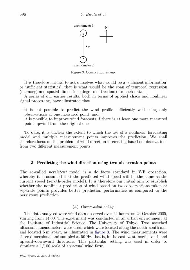
Figure 3. Observation set-up.

Y. Hirata et al.596

It is therefore natural to ask ourselves what would be a ‘sufficient information’or ‘sufficient statistics’, that is what would be the span of temporal regression(memory) and spatial dimension (degrees of freedom) for such data.

A series of our earlier results, both in terms of applied chaos and nonlinearsignal processing, have illustrated that

— it is not possible to predict the wind profile sufficiently well using onlyobservations at one measured point; and

— it is possible to improve wind forecasts if there is at least one more measuredpoint upwind from the original one.

To date, it is unclear the extent to which the use of a nonlinear forecastingmodel and multiple measurement points improves the prediction. We shalltherefore focus on the problem of wind direction forecasting based on observationsfrom two different measurement points.

3. Predicting the wind direction using two observation points

The so-called persistent model is a de facto standard in WF operation,whereby it is assumed that the predicted wind speed will be the same as thecurrent speed (zeroth-order model). It is therefore our initial aim to establishwhether the nonlinear prediction of wind based on two observations taken atseparate points provides better prediction performance as compared to thepersistent prediction.

(a ) Observation set-up

The data analysed were wind data observed over 24 hours, on 24 October 2005,starting from 14.00. The experiment was conducted in an urban environment atthe Institute of Industrial Science, The University of Tokyo. Two matchedultrasonic anemometers were used, which were located along the north–south axisand located 5 m apart, as illustrated in figure 3. The wind measurements werethree-dimensional and sampled at 50 Hz, that is, in the east–west, north–south andupward–downward directions. This particular setting was used in order tosimulate a 1/100 scale of an actual wind farm.

Phil. Trans. R. Soc. A (2008)

597Wind direction modelling

For the preprocessing of the data, a moving average filter on 2 s windows wasused, the data were then resampled at 2 s intervals. For convenience, we ignoredthe upward–downward direction and conducted our analysis only in the planespanned by the east–west and north–south direction.

Figure 4 and table 1 provide a comprehensive account of the statistics for the24 hours of wind data considered. Both quantitative and qualitative measuresdescribing such a process (including spatial distributions) are illustrated.

Figure 4a illustrates wind as a vector field, described by its speed and direction.Alternatively, we can base our modelling on the projections of this vector on thenorth and east axes. The representation for wind also depends on the way winddata are recorded: standard cup anemometers provide the speed–directioninformation, whereas modern ultrasonic instruments have a much wider range ofoptions. This is illustrated in figure 4b, where by inspection, wind was relativelystrong in the intervals between 14.00 and 16.00; 22.00 and 02.00; and 10.00 and14.00 (figure 4b(i)(ii)). As for the wind direction, figure 4b(iii) shows that between22.00 and 02.00 and between 10.00 and 14.00, the dominant wind direction wasfrom the north, whereas between 14.00 and 16.00, the dominant wind directionwas from the south.

A more convenient way to visualize these four time series is shown in figure 4c,in the form of wind lattice (wind rose similar to figure 2), where for every timeinstant the tip of the wind vector is represented by a dot. Observe a clear couplingbetween strong winds and the north–south direction. To further depict the rangeof wind directions, the histogram of figure 4d exhibits two peaks: the peakassociated with the easterly wind is related to the quiet periods between 18.00 and22.00 and between 02.00 and 10.00. The peak related to the northerly wind isrelated to high winds between 22.00 and 02.00 and between 10.00 and 14.00.

Theautocorrelationbasedonthe increments ofwinddirection fromfigure4e showsanticorrelation at a lag between 2 and 6 s. Owing to the experiment having beenconducted in an urban environment, for approximately 40% of the measured time,the wind speed was rather low and in the range between 0 and 0.2 m sK1 as shown inthe histogram in figure 4f. The variation of the wind speed showed large fluctuationssince the mean speed and its standard deviation were almost equal (table 1).

From the above analysis, it is clear that it is the forecasting of the winddirection that will have a major contribution in the intelligent operation of a WT.Since our underlying aim is to predict the wind direction, a straightforwardapproach would be to construct a prediction model based on the past values of thewind direction only. However, since wind speed and direction are coupled, ourproposed model will take advantage of the available wind speed information, inorder to predict direction only. The schematic graph is shown in figure 5. This taskmay be considered within the framework of experimental chaos. In fact, theembedding parameters and the different wind dynamics have been analysed in ourprevious work (Goh et al. 2006).

Let y1,1(t) and y1,2(t) be the wind direction and speed at time t for anemometer 1(A1) and y2,1(t) and y2,2(t) those for anemometer 2 (A2), and let us consider amodel that predicts the future wind direction at A2 based on the observed winddirection and speed from both the north and south (A1 and A2), as illustrated infigure 3. Based on an extension of the approach proposed by Judd and Mees(Hirata et al. 2006b), the maximum delay of 60 s was used for each element of y;the initial ‘optimal’ set z(t) of such delays used in the prediction can therefore be

Phil. Trans. R. Soc. A (2008)

(a) (b)

N

E

wind speedwinddirection

–202 (i)

(ii)

(iii)

(iv)

–5

0

5

0

180

360

(deg

.)

14.00 18.00 22.00 02.00 06.00 10.00 14.000

5(m

s–1)

(ms–1

)(m

s–1)

(c)

(e) ( f )

5 4 3 2 1 0 –1 –2 –3 –4 –55

4

3

2

1

0

–1

–2

–3

–4

–5

east wind (ms–1)

nort

h w

ind

(ms–1

)

(d )

0.05

0.1

easterly wind

northerly wind

0 10 20 30 40–0.5

0

0.5

1.0

lag (s)

auto

corr

elat

ion

coef

fici

ents

2 4 60

0.1

0.2

0.3

0.4

0.5

wind speed (ms–1)

rela

tive

freq

uenc

y

Figure 4. Quantitative and qualitative wind descriptors: (a) wind vector representation, (b(i)) timeseries of the easterly wind, (ii) northerly wind, (iii) wind direction and (iv) wind speed, (c) windrose representation, (d ) relative frequencies for wind direction, (e) autocorrelation based onincrements of wind direction of 2 s and ( f ) relative frequencies calculated for wind speed.

Y. Hirata et al.598

Phil. Trans. R. Soc. A (2008)

Table 1. Statistical properties of the dataset.

minimum speed 0 (m sK1)maximum speed 5.25 (m sK1)mean speed 0.41 (m sK1)standard deviation of speed 0.44 (m sK1)

direction

1 2 t

prediction modelt+p

time

predictionspeed

direction

speed

south

north

Figure 5. Illustration of the direction–speed model.

599Wind direction modelling

expressed as

zðtÞZ ðy1;1ðtK t1;1;1Þ; y1;1ðtK t1;1;2Þ;.; y1;1ðtK t1;1;k1;1Þ;y1;2ðtK t1;2;1Þ; y1;2ðtK t1;2;2Þ;.; y1;2ðtK t1;2;k1;2Þ;y2;1ðtK t2;1;1Þ; y2;1ðtK t2;1;2Þ;.; y2;1ðtK t2;1;k 2;1

Þ;y2;2ðtK t2;2;1Þ; y2;2ðtK t2;2;2Þ;.; y2;2ðtK t2;2;k 2;2

ÞÞ:

ð3:1Þ

To facilitate the nonlinear mode of operation, we next investigate an affineCradialbasis function model with 100 radial basis functions as proposed by Judd & Mees(1995) with the normalized maximum likelihood (Rissanen 2000) as theinformation criterion.

There are two basic ways of multiple step ahead prediction: the direct anditerated mode, where the iterated mode suits feedback prediction models. Owing tothe choice of our computing model, we used direct predictions, for which p stepahead prediction model has the form of

y2;1ðtCpÞzfpðzðtÞÞZ apCbp$zðtÞCX100jZ1

cp;jexp KjjzðtÞKdp;j jj2

2s2p

!; ð3:2Þ

where ap, bp, cp,j, dp,j and sp are parameters of the model.In the model evaluation set-up, the performance of the proposed direction–speed

model was compared to that of a persistent model, for which the wind direction at2 s before the actual point of interest was used as a persistent prediction.

Our proposedmodel was built based upon the first 2000 points of the data and theperformance was evaluated on the subsequent 200 data points. To cover all theavailable data, these data windows were shifted by 200 points after every predictionand this process was repeated for 206 times.

Phil. Trans. R. Soc. A (2008)

20 40 60 80 1000

20

40

60

80

100

r.m.s.e. for persistent model

r.m

.s.e

. for

dir

ectio

n an

d sp

eed

mod

el

Figure 6. Scatter diagram illustrating the performance of the persistent and direction–speed modelfor a one step ahead prediction task. Each point corresponds to a prediction window. Thehorizontal axis is the root mean square error (r.m.s.e.) for the persistent model and the vertical axiscorresponds to the r.m.s.e. for the direction–speed model. This way, if the r.m.s.e. for the persistentmodel is smaller than that for direction–speed model, the resulting point in the scatter diagram willbe above the bisector line.

Y. Hirata et al.600

The performance comparison shown in figure 6 shows that for this rather rawcase, the persistent model exhibited better performance than the proposeddirection–speed model. This result may be explained by the fact that the directionsignal has a circular nature, hence experiencing problems around the singularpoints, where such prediction is totally unreliable.

(b ) The two-dimensional model

To overcome the problem with the discontinuity associated with a circularnature of wind direction, we propose a two-dimensional model, whereby the windscoming from east and north were predicted at the south anemometer and then thewind directions were calculated from these predictions. The predictions were basedon the observations from both the south and north anemometer (figure 7). Theprocedures for making a predictive model were the same as those used in thespeed–direction model. We found that the two-dimensional model was likely to bebetter than the persistent model as illustrated in figure 8a, where the majority ofthe points are located below the bisector line. This result is consistent with ourprevious study (Hirata et al. 2006a), where the observations from the predictedpoint only were used for the prediction. Even in the case of a 20 s ahead directprediction, this tendency continued (figure 8b). Over all the tested intervals, thetwo-dimensional model showed tendency to have a smaller prediction error thanthe persistent model. In figure 9, the probability that the two-dimensional modelhas a smaller prediction error than the persistent model is above 0.5 for all thetested prediction horizons, thus indicating superiority of the two-dimensionalmodel over the persistent model. The direction–speed model exhibited worseperformance than the persistent model when the prediction horizon was lessthan 5 s.

Phil. Trans. R. Soc. A (2008)

north windat south

1 2 t

prediction model

time prediction for t+p

north windat north

east windat south

east windat north

direction at t+p

Figure 7. Block diagram of the proposed two-dimensional model.

(a)

5 10 15 20 25 30 35 40

10

15

20

25

30

35

40

r.m

.s.e

. for

two

dim

ensi

onal

mod

el

(b)

0 10 20 30 40 50 60 70 80 90

10

20

30

40

50

60

70

80

90

r.m.s.e. for persistent model

r.m

.s.e

. for

two

dim

ensi

onal

mod

el

Figure 8. Performance of the two-dimensional model for (a) 2 s and (b) 20 s ahead prediction. Thehorizontal axis is the root mean square error (r.m.s.e.) for the persistent model and the vertical axiscorresponds to the r.m.s.e. for the two-dimensional model. In both the figures, more points are locatedbelow the bisector line, indicating that the two-dimensional model showed better performance than thepersistent model.

601Wind direction modelling

Phil. Trans. R. Soc. A (2008)

5 10 15 20 250

0.2

0.4

0.6

0.8

1.0

prediction horizon (s)

mer

it fi

gure

for

the

prop

osed

mod

el two-dimensional

direction and speed model

Figure 9. Comparison of the prediction performance between the proposed and persistent model.Letting m be the number of windows for which the prediction error is smaller than that of thepersistent model and n the total number of windows, we calculated the ratio m/n for eachprediction horizon.

Y. Hirata et al.602

4. Factors in the prediction of the wind direction

The performance of a prediction model heavily leans on the amount and spatialdistribution of the data, number of observation points and the choice of model(linear and nonlinear).

(a ) Choice of the number of measurement points

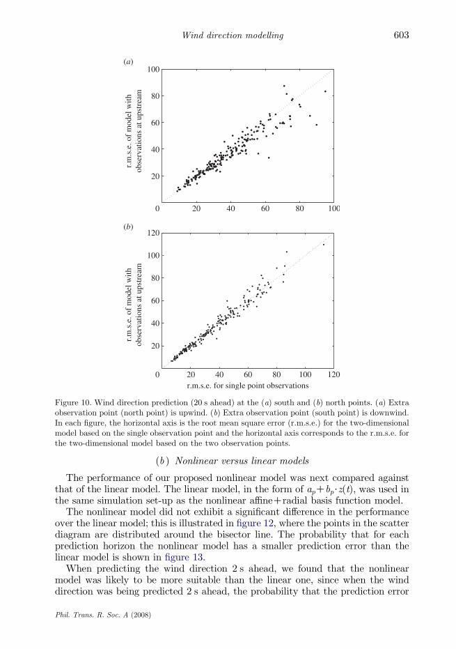
Closely related to the concept of data fusion and sufficient information (Mandicet al. 2007), we have gathered both the theoretical and empirical evidence that theprediction performance improved when measurements from two spatiallydistributed anemometers were used. Indeed, for the wind direction predictionexperiment for the south anemometer, the additional information coming from thenorth anemometer improved the prediction error. This is illustrated in figure 10a,where the majority of the points are below the bisector line. On the other hand,when the wind direction at the north anemometer was predicted based on themeasurements from the north and south anemometer, the second set ofobservations coming from the south point did not improve the prediction, asillustrated in figure 10b.

Over all the tested prediction intervals, the second observation coming fromupwind enhanced the prediction: according to figure 11, when using additionalobservations upwind, the probability that themodel using observations upwindhasa smaller prediction errorwas always above 0.5.Whenobservations fromdownwindwere taken, the probability that the model using those observations has a smallerprediction error than thatwithout themwas approximately 0.5. It therefore did notmake much difference whether the downwind observations were used.

Phil. Trans. R. Soc. A (2008)

(a)

20 40 60 80 1000

20

40

60

80

100

r.m

.s.e

. of

mod

el w

ithob

serv

atio

ns a

t ups

trea

m

(b)

20 40 60 80 100 1200

20

40

60

80

100

120

r.m.s.e. for single point observations

r.m

.s.e

. of

mod

el w

ithob

serv

atio

ns a

t ups

trea

m

Figure 10. Wind direction prediction (20 s ahead) at the (a) south and (b) north points. (a) Extraobservation point (north point) is upwind. (b) Extra observation point (south point) is downwind.In each figure, the horizontal axis is the root mean square error (r.m.s.e.) for the two-dimensionalmodel based on the single observation point and the horizontal axis corresponds to the r.m.s.e. forthe two-dimensional model based on the two observation points.

603Wind direction modelling

(b ) Nonlinear versus linear models

The performance of our proposed nonlinear model was next compared againstthat of the linear model. The linear model, in the form of apCbp$z(t), was used inthe same simulation set-up as the nonlinear affineCradial basis function model.

The nonlinear model did not exhibit a significant difference in the performanceover the linear model; this is illustrated in figure 12, where the points in the scatterdiagram are distributed around the bisector line. The probability that for eachprediction horizon the nonlinear model has a smaller prediction error than thelinear model is shown in figure 13.

When predicting the wind direction 2 s ahead, we found that the nonlinearmodel was likely to be more suitable than the linear one, since when the winddirection was being predicted 2 s ahead, the probability that the prediction error

Phil. Trans. R. Soc. A (2008)

0 5 10 15 20 250.45

0.50

0.55

0.60

0.65

0.70

0.75

prediction horizon (s)

mer

it fi

gure

for

the

prop

osed

met

hod

ratio m/n using observations upwind

ratio m/n using observations downwind

Figure 11. Comparison of the prediction performance between the two-dimensional model based ontwo observation points and that based on a single observation point. Letting m be the number ofwindows for which the prediction error for the model using observations upwind (downwind) issmaller than that obtained without them and n being the total number of windows, we calculatedthe ratio m/n for each prediction horizon.

20 40 60 80 1000

20

40

60

80

100

r.m.s.e. for linear model

r.m

.s.e

. for

non

linea

r m

odel

Figure 12. Comparison of the linear and nonlinear wind direction prediction models at the southpoint using our two-dimensional model and observations at both points (20 s ahead). Thehorizontal axis is the root mean square error (r.m.s.e.) of linear model and the vertical axiscorresponds to the r.m.s.e. of nonlinear model.

Y. Hirata et al.604

for the nonlinear model was smaller than that for the linear model was above 0.5.This tendency was also observed in other datasets. In the short time ranges, theincrements for the wind direction are anticorrelated (figure 4e) and thenonlinearity of the short-term prediction may be due to this anticorrelation.

Phil. Trans. R. Soc. A (2008)

0 5 10 15 20 25

0.35

0.40

0.45

0.50

0.55

0.60

prediction horizon (s)

mer

it fi

gure

for

the

nonl

inea

r m

odel

Figure 13. Comparison of the prediction performance between the nonlinear and linear model.Letting m be the number of windows for which the prediction error for the nonlinear model issmaller than that for the linear model and n the total number of windows, we calculated the ratiom/n for each prediction horizon.

0 0.5 1.0 1.5 2.0 2.5 3.0 3.5 4.0–0.2

0

0.2

0.4

0.6

0.8

1.0

wind speed (ms–1)

outp

ut (

arb.

uni

t)

Figure 14. First approximation of the power curve from figure 1.

605Wind direction modelling

5. Benefits of the proposed nonlinear multiobservation model

Although the difference in the prediction errors between the two-dimensional andpersistent model was small, this produced a significant difference in the expectedelectricity production. To quantify this, in the following simulation, we used thepredicted wind directions and speeds for the control of a wind turbine andsubsequently estimated the expected amount of produced electricity using the actualdata. In the simulation, we used the simplified power curve given in figure 14.

Phil. Trans. R. Soc. A (2008)

Table 2. Expected electricity production from each combination of methods.

direction speed energy estimated (arb. unit)

speed–direction speed–direction 1546.9persistent persistent 1608.7two-dimensional persistent 1611.3persistent two-dimensional 1690.2two-dimensional two-dimensional 1721.9

Y. Hirata et al.606

In this experiment, we also compared some existing methods, as shown intable 2 where when two-dimensional models were used for the modelling of winddirections and speeds, the improvement in the total amount of energy was 7% inthe case when the persistent models were used for predicting the wind directionsand speeds, and 2% in the case when using the persistent model for predicting thewind directions and the two-dimensional model for predicting wind speeds.

6. Conclusions

We have introduced a novel theoretical and experimental framework for theprediction of wind direction based on a two-dimensional wind vector representation.The benefits of the proposed approach are based on the use of two observationpoints which has led to the consistently improved performance as compared to thepersistent model. Although the difference in quantitative performance between theproposed method and the persistent prediction is relatively small, this makes asignificant difference in the expected production of electricity.

This study was partially supported by the Industrial Technology Research Grant Program in 2003,from the New Energy and Industrial Technology Development Organization (NEDO) of Japan. Thework of D.P.M. was supported by EPSRC (EP/D061709/1).

References

Aihara, K. 2002 Chaos engineering and its application to parallel distributed processing with chaoticneural networks. Proc. IEEE 90, 919–930. (doi:10.1109/JPROC.2002.1015014)

Aihara, K & Katayama, R. 1995 Chaos engineering in Japan. Commun. ACM 38, 103–107. (doi:10.1145/219717.219801)

Gautama, T., Mandic, D. P. & Van Hulle, M. M. 2003 On the indications of nonlinear structures inbrain electrical activity. Phys. Rev. E 67, 046204. (doi:10.1103/PhysRevE.67.046204)

Gautama, T., Mandic, D. P. & Van Hulle, M. M. 2004 The delay vector variance method fordetecting determinism and nonlinearity in time series. Physica D 190, 167–176. (doi:10.1016/j.physd.2003.11.001)

Goh, S. L. & Mandic, D. P. 2004 A complex-valued RTRL algorithm for recurrent neural networks.Neural Comput. 16, 2699–2713. (doi:10.1162/0899766042321779)

Goh, S. L. & Mandic, D. P. 2005 Nonlinear adaptive prediction of complex-valued signals by complex-valued PRNN. IEEE Trans. Signal Process. 53, 1827–1836. (doi:10.1109/TSP.2005.845462)

Goh, S. L., Chen,M., Popovic, D. H., Aihara, K., Obradovic, D.&Mandic,D. P. 2006Complex-valuedforecasting of wind profile. Renew. Energ. 31, 1733–1750. (doi:10.1016/j.renene.2005.07.006)

Phil. Trans. R. Soc. A (2008)

607Wind direction modelling

Hirata, Y., Suzuki, H., Aihara, K., Abe, R., Kanie, K., Yamada, T. & Takahashi, J. 2004 Looking fornonlinearity in the dynamics of surface wind using surrogate data. In Proc. 2004 Int. Symp.on Nonlinear Theory and its Applications (NOLTA 2004), Fukuoka, Japan, November 2004,pp. 207–210.

Hirata, Y., Suzuki, H. & Aihara, K. 2005 Predicting the wind using spatial correlation. In Proc. 2005Int. Symp. on Nonlinear Theory and its Applications (NOLTA 2005), Bruges, Belgium, October2005, pp. 634–637.

Hirata, Y., Suzuki, H. & Aihara, K. 2006a Predicting wind direction using nonlinear models and timeseries data. In 2006 Annual Meeting Record I.E.E. Japan, vol. 7, p. 87.

Hirata, Y., Suzuki, H. & Aihara, K. 2006b Reconstructing state spaces from multivariate data usingvariable delays. Phys. Rev. E 74, 026202. (doi:10.1103/PhysRevE.74.026202)

Hirata, Y., Horai, S., Suzuki, H. & Aihara, K. 2007 Testing serial dependence by Random-shufflesurrogates and the Wayland method. Phys. Lett. A 370, 265–274. (doi:10.1016/j.physleta.2007.05.061)

Judd, K. & Mees, A. 1995 On selecting models for nonlinear time series. Physica D 82, 426–444.(doi:10.1016/0167-2789(95)00050-E)

Kantz, H. & Schreiber, T. 2003 Nonlinear time series analysis. Cambridge, UK: CambridgeUniversity Press.

Kantz, H., Holstein, D., Ragwitz, M. & Vitanov, N. K. 2004aMarkov chain model for turbulent windspeed data. Physica A 342, 315–321. (doi:10.1016/j.physa.2004.01.070)

Kantz, H., Holstein, D., Ragwitz, M. & Vitanov, N. K. 2004b Extreme events in surface wind:predicting turbulent gusts. In Proc. 8th Experimental Chaos Conference, Florence, Italy, 14–17June 2004, vol. 742 (ed. S. Boccaletti). AIP Conference Proceedings, pp. 315–324. New York, NY:American Institute of Physics.

Lorenz, E. N. 1963 Deterministic nonperiodic flow. J. Atmos. Sci. 26, 130–141. (doi:10.1175/1520-0469(1963)020!0130:DNFO2.0.CO;2)

Mandic, D. P., Goh, S. L. & Aihara, K. 2007 Sequential data fusion via vector spaces: fusion ofheterogeneous data in the complex domain. Int. J. VLSI Signal Process. Syst. 48, 99–108. (doi:10.1007/s11265-006-0025-6)

Manwell, J. F., McGowan, J. G. & Rogers, A. L. 2002 Wind energy explained: theory, design andapplication. New York, NY: Wiley.

Ragwitz, M. & Kantz, H. 2000 Detecting non-linear structure and predicting turbulent gusts insurface wind velocities. Europhys. Lett. 51, 595–601. (doi:10.1209/epl/i2000-00379-x)

Rissanen, J. 2000 MDL denoising. IEEE Trans. Inform. Theory 46, 2537–2543. (doi:10.1109/18.887861)

Roulston, M. S., Kaplan, D. T., Hardenberg, J. & Smith, L. A. 2003 Using medium-range weatherforecasts to improve the value of wind energy production. Renew. Energ. 28, 585–602. (doi:10.1016/S0960-1481(02)00054-X)

Phil. Trans. R. Soc. A (2008)