Page 1 of 35

Wildland/Urban Interface and Communities at Risk

Joint Fire Modeling ProjectBureau of Land Management, Upper Snake River District GIS

AndIdaho State University GIS Training and Research Center

08-16-2002

Cecilia Jansson, cecjan-9@student.luth.se Computer: AbsarokaOskar Pettersson, oskpet-9@student.luth.se Computer: Snake

Abstract: Wildland/Urban Interface (WUI) and Communities at Risk (CAR) are high priorities tofederal land management agencies. It is important that the federal government help educatehomeowners, firefighters, local officials and land managers regarding the value and risk ofwildland fire. The Bureau of Land Management (BLM) Upper Snake River District (USRD)Geographic Information Systems (GIS) team in cooperation with GIS Training and ResearchCenter (GISTReC) at Idaho State University (ISU) have created a model to predict potentialwildfire risk areas for Lava Hot Springs, Idaho and vicinity.

During this project we created maps of wildland/urban interface areas, identified structuresencroaching on wildland risk areas, mapped road access and potential response times, predictedsuppression methodologies, and identified areas at risk.

This report describes each component of our wildfire risk model and what effect each had on thefinal wildfire risk model. We hope the information will benefit future users of this model and willhelp the people in the Lava Hot Springs area better protect themselves against wildfire.

Keywords: Fire, Wildfire, GIS, WUI (Wildland/Urban Interface), Lava Hot Springs

Page 2 of 35

Content: PageAbstract 1Keywords 1Introduction 2Methods 3

Creating NDVI models 3GAP verses NDVI 4Fuel load Model 4Create wildfire model components 4Fuel load/Vegetation moisture 4Fuel load/Rate of spread 7Fuel load/ Intensity 8Slope 9Slope/Rate of spread 9Slope/Suppression difficulties 10Aspect 11Aspect/Sun position and daily temperature 11Response time 12WUI fire risk model 12Adding fires occurring after 1999 13

Results 14Discussion 26Assessment of errors and bias 27Reference cited 27Acknowledgments 27Appendix A 28Appendix B 32Appendix C 34Appendix D 35

Introduction: Fire and related agencies first begun to use GIS as a way of sharing and managinginformation about natural resources. In the mid-1990s the trend culminated and many federal,state, and local wildfire agencies began conducting protection assignments. The CaliforniaDepartment of Forestry and Fire Protection published a fire plan. The idea was to trainfirefighters with experience in the field to use GIS, Amdahl (2001).

This study examined wildland/urban interface (WUI) fire risk for the Town of Lava Hot Springs,Idaho and neighboring areas. It was conducted to produce a WUI risk model using GIS. This is acontinuation of the WUI project that began by examining the City of Pocatello. Results can beused by firefighters, homeowners, land managers, and as public information to prevent andmanage wildfire. The model predicts wildfire risk in the Lava Hot Springs area. There have beenearlier studies but typically, these had a more generalized approach. One example is the FireArea Simulator Model Development and Evaluation (FARSITE).

Page 3 of 35

Methods: We acquired and assembled the GIS data sets needed for our area of interest (AOI).The area was defined as the area encompassed by the Bancroft, Haystack Mountain, Lava HotSprings, and Sedgwick Peak 7.5’ USGS quadrangles. To utilize the data, we projected anddefined each data set as needed.

Required data:

- Vegetation (Idaho GAP and Landsat 7 ETM+ derived NDVI-based classification)- Geocoded roads- Wildfire Fuel load model- Emergency Response Time model (ERT)- Digital Raster Graphics (DRG)- Digital Elevation Models (DEM)- Digital Orthophoto Quarter-Quads (DOQQ)- Landsat 7 ETM+ imagery- Fire Station location

To produce one DEM for the AOI, we merged Bancroft, Haystack Mountain, Lava Hot Springsand Sedgwick Peak DEM-quadrangles into one grid using ArcInfo Workstation à GRID àmosaic. Using the spatial extent defined by the footprint of this grid, we created a “cookiecutter”, a polygon coverage called aoi_lava. All the data sets listed above were clipped using the“cookie cutter” as needed.

We reclassified vegetation data into three categories (Paved Urban, Fire-Prone Vegetation, andHigh moisture Vegetation) using ArcMap à Spatial analyst à reclassify.

We defined the projection of all data sets as Idaho Transverse Mercator (GCS North American1927) using Arc Toolbox à define.

Creating NDVI modelsWe located vegetation of interest with satellite imagery using the Normalized DifferenceVegetation Index (NDVI) for Landsat 7. We used Landsat 7 ETM+ imagery dated 08-23-2000.The NDVI uses Red and Near Infrared (NIR) bands. We ratioed these bands following theequation given in figure 1.

redNIRredNIRNDVI

+−=

Figure 1: How we calculated NDVI.

The NDVI has an interval of –1 to +1, where –1 is no vegetation and +1 is purephotosynthetically active vegetation. Our tests have shown that values > 0.3 reliably indicatephotosynthetically active vegetation (Ben McMahan pers. comm.).

We made several raster calculations of the NDVI grid. The first showed all values > 0, the nextshowed values >0.05, etc (i.e., 0, 0.05, 0.1, 0.15, 0.2, 0.25, 0.3). The calculations were made inArcMap à Spatial Analyst à Raster Calculator. After making the resulting grids, we comparedeach of them with the DOQQ’s.

Page 4 of 35

GAP verses NDVITo test the agreement between the GAP and NDVI vegetation models, we multiplied each of theNDVI grid results (described above) with the GAP vegetation grid. The calculations were madein ArcInfo Workstation as a map algebra operation.

The NDVI grid includes both areas with and without vegetation. We needed to determine theNDVI value that approximated a threshold separating between non-vegetation and vegetationareas. We did this by again comparing the DOQQ’s with the values within the NDVI grid (in thiscase -0.35056 - +0.75581). Using the same method, we separated dry vegetation and moistvegetation. We weighted the 3 NDVI classes: No vegetation = 1, Dry vegetation = 2, Moistvegetation = 0.75 in ArcMap à Spatial Analyst à Reclassify. ArcMap’s reclassify can notcreate an outgrid with floating points, so we multiplied the weights with 100 (integer values).

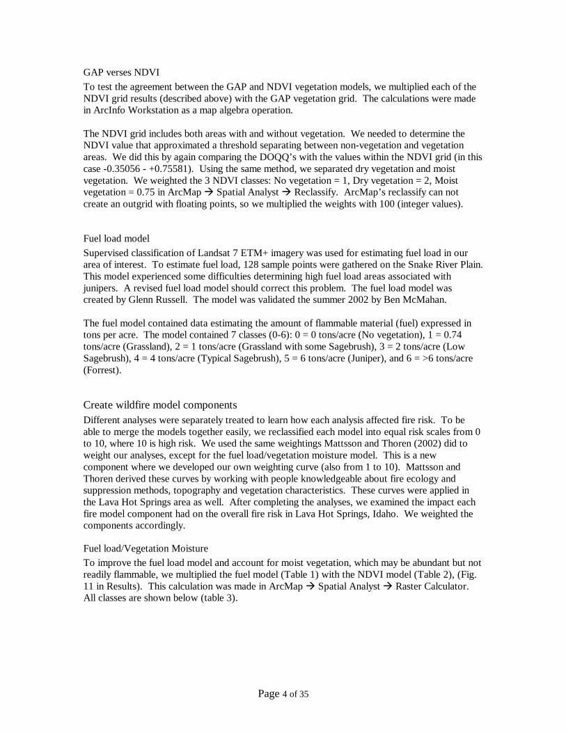
Fuel load modelSupervised classification of Landsat 7 ETM+ imagery was used for estimating fuel load in ourarea of interest. To estimate fuel load, 128 sample points were gathered on the Snake River Plain.This model experienced some difficulties determining high fuel load areas associated withjunipers. A revised fuel load model should correct this problem. The fuel load model wascreated by Glenn Russell. The model was validated the summer 2002 by Ben McMahan.

The fuel model contained data estimating the amount of flammable material (fuel) expressed intons per acre. The model contained 7 classes (0-6): 0 = 0 tons/acre (No vegetation), 1 = 0.74tons/acre (Grassland), 2 = 1 tons/acre (Grassland with some Sagebrush), 3 = 2 tons/acre (LowSagebrush), 4 = 4 tons/acre (Typical Sagebrush), 5 = 6 tons/acre (Juniper), and 6 = >6 tons/acre(Forrest).

Create wildfire model componentsDifferent analyses were separately treated to learn how each analysis affected fire risk. To beable to merge the models together easily, we reclassified each model into equal risk scales from 0to 10, where 10 is high risk. We used the same weightings Mattsson and Thoren (2002) did toweight our analyses, except for the fuel load/vegetation moisture model. This is a newcomponent where we developed our own weighting curve (also from 1 to 10). Mattsson andThoren derived these curves by working with people knowledgeable about fire ecology andsuppression methods, topography and vegetation characteristics. These curves were applied inthe Lava Hot Springs area as well. After completing the analyses, we examined the impact eachfire model component had on the overall fire risk in Lava Hot Springs, Idaho. We weighted thecomponents accordingly.

Fuel load/Vegetation MoistureTo improve the fuel load model and account for moist vegetation, which may be abundant but notreadily flammable, we multiplied the fuel model (Table 1) with the NDVI model (Table 2), (Fig.11 in Results). This calculation was made in ArcMap à Spatial Analyst à Raster Calculator.All classes are shown below (table 3).

Page 5 of 35

Table 1 Table 2

Table 3 Table 4

As we did not have a curve for this model, we developed weightings for all classes with Keith T.Weber (Table 4). The weightings are based on worst case scenario and so are conservative. Ifthere could be more than one solution, (e.g., class 2, that can be both 1 tons/acre * 2 (a little fueland dry vegetation) and 2 tons/acre * 1 (more fuel but no vegetation predicted)) we calculatedwith the worst scenario. By worst criteria we mean that, if we had class 6 (Table 3), which can beboth 3 tons/acre *2 or 6 tons/acre *1, we used 3*2 when we weighted class 6 because 3*2 has ahigher fire risk than 6*1 and therefore was the worst case. We did that for all 15 classes, andtried to balance every class to find the correct weights for them (fig 2, table 6 in Appendix B).

Page 6 of 35

Figure 2. This chart describes all weightings for fuel load/moist vegetation.

Page 7 of 35

Fuel load/Rate of SpreadHow fast a fire will spread depends on the amount of continuous fuels and other factors. Thelower fuel load classes were considered to be the primary carrier of fire (e.g. grasser), and havethe fastest spread rate. The higher fuel load classes will not burn as quickly because as moisturecontent increases, spread rate is reduced. We reclassified the Fuel load model following Mattssonand Thoren, 2002 (table 7 in Appendix B), using ArcMap à Spatial Analyst à Reclassify (fig3).

Figure 3. Weightings for Fuel load/Rate of Spread describe how the fuel load affects the fire spread rate.

Page 8 of 35

Fuel load/IntensityIntensity is considered the amount of energy a fire produces. The more energy the fire produces,the more difficult it is for the firefighters to suppress it. Intensity depends on fuel load and otherfactors such as wind and ground conditions at the time of the fire. We reclassified the Fuel loadmodel using values following Mattsson and Thoren (table 8 in Appendix B) using ArcMap àSpatial Analyst à Reclassify (Fig 4).

Figure 4. Weightings for the Fuel load/Intensity describes how the fire intensity depend on the fuel load.

Page 9 of 35

SlopeSlope is a matter of degree and stability of surface. The extent and intensity of a wildfire dependson the topography of the land it is burning up. When fire moves across flat land it moves moreslowly then fire on a mountainside. However, the fire moves much faster up hill then down hill,so you can say, the steeper the slope, the faster the fire, Amdahl (2001).

Using the merged DEM-quadrangles aoi_lavadem, we made a slope grid that calculated howsteep the surface is using ArcMap à Spatial Analyst à Surface Analysis à Slope.

Output measurement: degreeZ-factor: 1Output cellsize: 30

Slope/Rate of SpreadTo make the Slope/Rate of Spread model, we weighted the result of the slope model(aoi_lavaslope) by using weightings for slope/rate of spread from table 9 in Appendix B(Mattsson and Thoren, 2002) in ArcMap à Spatial Analyst à Reclassify. As the reclassifiedgrid must be integer, we multiplied all weights by100 (we did this with all fire modelcomponents). Slope/Rate of Spread shows spread rate that is dependent on slope (i.e., the steeperthe terrain is, the higher the fire risk is (fig 5)).

Figure 5. Weightings describe how spread rate increase by the angle of slope. The weight proportion isassumed to be exponentially with slope angle.

Page 10 of 35

Slope/Suppression DifficultiesFor the Slope/Suppression Difficulties model, we used the original slope grid once again, butapplied weighting data for slope/suppression difficulties following Mattsson and Thoren, 2002(table 10 in Appendix B). ArcMap à Spatial Analyst à Reclassify (fig 6). Slope/SuppressionDifficulties shows how difficult it is for firefighters to fight fire based on slope. If firefighterscannot reach the fire, it will keep burning even though it may be a low risk area according toother criteria.

Figure 6. Weightings for slope/suppression difficulties describe how suppression difficulties are affectedby the angle of slope.

Page 11 of 35

AspectAspect shows what direction the surface faces. We made the aspect model from aoi_lavadem inArcMap à Spatial Analyst à Surface Analysis à Aspect.

Output cellsize: 30

Aspect/Sun position and daily temperatureAspect/Sun position and daily temperature illustrates the direction the slope is facing and wherethe sun affects the ground/vegetation most. The sun is predicted to desiccate theground/vegetation more on the southerly aspects than others. We reclassed the aspect grid(aoi_lavaasp) in ArcMap à Spatial Analyst à Reclassify (fig 7 and table 11 in Appendix B).

Figure 7. Weightings for Aspect/Sun position and daily temperature describe how the sun desiccates the ground more in south facing aspects and therefore get higher risk.

Page 12 of 35

Response TimeThe fire station in Lava Hot Springs is a volunteer fire station. Because it is a volunteer firestation, it is unstaffed. Thus it will take a while for the firefighters to respond to an emergency.According to Lava Hot Springs fire chief Joel Price it will take the firefighters 1 – 2 minutes toarrive at the station and up to five minutes to respond.

The weightings for the response time model Mattsson and Thoren, 2002 (table 12 in Appendix B)are based on the time frame from when a house catches fire until it flashes over (fig. 8). Theweightings describe how the fire risk due to delayed travel time for the firefighters influences therisk. Because it takes the firefighters 5 minutes to respond, the entire Lava Hot Springs area has aresponse time risk of 10. Since the entire area of interest is in the highest risk, there are novariations in the response time model. Therefore we did not need it for the final model, but havemade a response time model for cartographic purposes.

Figure 8. The weightings describe how the fire risk due to delayed travel time for the firefightersinfluences the risk.

Page 13 of 35

WUI fire risk modelAfter estimating the different fire model components, we decided how important each componentwas to the overall fire risk model. Beginning with the highest, we distributed the components asfollows:

• Fuel load/Rate of Spread 25% (of total fire risk model)

• Fuel load/Vegetation Moisture 23%

• Fuel load/Intensity 20%

• Slope/Suppression Difficulties 17%

• Slope/Rate of Spread 10%

• Aspect/Sun position and Daily temperature 5%

After this, we added the individual components together in ArcMap à Spatial Analyst à RasterCalculator, to produce a final WUI fire risk model.

Adding fires occurring after 1999After merging all the fire model components together we realized that our risk model did notinclude any fires occuring after 1999. Such recent fires drastically change an areas risk tosubsequent fires. The Bureau of Land Management (BLM) and ISU GIS TreC had datadescribing fires from 1939 to 2000. We selected the wildfires from 2000 using ArcMap à SelectFeatures, and then converted the resulting features to a grid by using ArcMap à Spatial Analystà Convert à Features to Raster.

Field: fire_freqOutput cellsize: 30

To get the wildfires for 2001, we again used a BLM wildfire coverage. We followed the sameprocedures as for the 2000 fires.

Field: wildfire-IDOutput cellsize: 30

Using the two recent wildfire grids (2000 and 2001), we added them together into a grid calledaoi_f00-01 where No Data was zero and fire pixels had a value of one. We reclassified it twice.First we produced a grid where we assigned fire pixels from both 2000 and 2001 the value zeroand No Data the value of one in ArcMap à Spatial Analyst à Reclassify. Then, when wemultiplied that mask grid with the complete fire risk model in ArcMap à Spatial Analyst àRaster Calculator, the new fires received a value of zero and all other data remained the same.The resulting grid was called “reset”. In the second reclassification, we gave the fire pixels avalue of one and No Data pixels a value of zero. We used ArcMap à Spatial Analyst àReclassify to accomplish this. We added this grid to reset in ArcMap à Spatial Analyst à RasterCalculator. The result is that new fires received a value of one “unclassified” and all other datadid not change. The final fire risk model was called “aoi_wui”.

Page 14 of 35

Results: All results are presented with the same approach as in Methods.

GAP verses NDVITo determine if the area was correctly classified by the GAP vegetation model, we compared theGAP vegetation grid (aoi_lavaveg) with DOQQ (fig. 9). We found there is vegetation in the areawhere the GAP vegetation grid (aoi_lavaveg) says it is “paved urban”.

Figure 9. Overlay of aoi_lavaveg and the DOQQ’s. This layout is made in ArcMap.

According to the GAP vegetation model (aoi_lavaveg) (fig. 9), the entire area around Lava HotSprings is “paved urban”. The NDVI (fig. 10) shows that it is not just “paved urban”, but also agood deal of vegetation. Since we had to choose one of these two grids for our vegetation model,we compared them as follows.

Page 15 of 35

The resulting NDVI grid (fig. 10) is a measure of the amount and vigor of vegetation.

Figure 10. The NDVI has an interval of –1 to +1, where –1 is no vegetation and +1 is pure vegetation.This layout was made in ArcMap.

The NDVI based model predicts vegetation more accurately than the GAP model, compared withthe DOQQ’s.

Comparing the values within the NDVI and the DOQQ’s, we found that all values <0.01represented no vegetation. Values between 0.10 and 0.17 represent dry vegetation and values>0.17 represent moist vegetation.

We next created a new grid from the NDVI grid where we gave all values <0.01 (no vegetation)the value of 100, all values between 0.01 and 0.17 (dry vegetation) the value of 200 and all values>0.17 (moist vegetation) the value of 75. This grid was called aoi_vegmodel.

Page 16 of 35

Fuel load/Vegetation moistureWe merged the reclassified NDVI (aoi_vegmodel) and the fuel model (aoi_lavafuel) (table 5),and completed one of the necessary analyses required to fully implement our model. The resultwas a grid with 15 classes (0, 0.75, 1, 1.5, 2, 2.25, 3, 3.75, 4, 4.5, 6, 8, 10, 12). Areas with value0 have a low fire risk (no vegetation and 0 tons of fuel/acre) and areas with value 12 have a highfire risk (dry vegetation and >6 tons of fuel/acre).

VegetationMoisture model

Fuel loadmodel

Result

100 200 75 1 4 6 100 800 450100 200 200 * 0 4 6 = 0 800 120075 200 100 3 6 5 225 1200 500Table 5. This is an example of what happens when you multiply the Vegetation

Moisture model (built using NDVI index) with the fuel load model.

Figure 11. This is our modified fuel load/vegetation moisture model (ndvi_fuelmod).

Page 17 of 35

Since there were no previous weightings for the fuel load/vegetation moisture model, wedeveloped our own weightings. Figure 2 in Methods shows how we weighted each class. Wealso created a map (fig 12) that shows how fuel load/vegetation moisture model affects fire risk inour study area using weights in figure 2.

Figure 12. This map shows how fuel load/vegetation moisture model affects fire risk.

Page 18 of 35

Remaining fire risk model componentsWe created a map (fig 13) that shows how the fuel load affects the fire spread rate in our studyarea.

Figure 13. This map shows how the rate of spread of fire is affected by fuel load.

Page 19 of 35

We created a map (fig 14) that shows how the intensity of a fire is affected by the fuel load in ourstudy area.

Figure 14. This map shows how the fire intensity is affected by the fuel load.

Page 20 of 35

We created a map (fig 15) that shows how rate of spread increases in areas with a steeper slopeand therefore these areas have a higher fire risk.

Figure 15. This map shows rate of spread depending on slope. The steeper the terrain is, the higherwill the fire risk be.

Page 21 of 35

We created a map (fig 16) that shows how suppression difficulties, depending on slope, affectsthe fire risk in our study area.

Figure 16. This map describes how the suppression difficulties increase on areas with a steeper slopethan areas not as steep. Therefore, those areas have a higher fire risk.

Page 22 of 35

We created a map (fig 17) that shows how the sun position and daily temperature affects firerisk in our study area.

Figure 17. This map shows how sun position and daily temperature affects the fire risk.

Page 23 of 35

We created a map (fig 18) that shows how response time affects the fire risk in our study area. Itdoes not have the same risk scale as the other fire model components. This because it takes thefirefighters in Lava Hot Springs 5 minutes to respond, which gives the whole area the highestrisk. This map is just for showing the risk depending on response time if Lava Hot Springs had anon-volunteer fire station.

Figure 18. This map shows how the response time is distributed in our study area.

Page 24 of 35

We created a map (fig 19) that shows the fire model components added together as a completeWUI risk model.

Figure 19. This map shows the result of all wildfire model components together.

Page 25 of 35

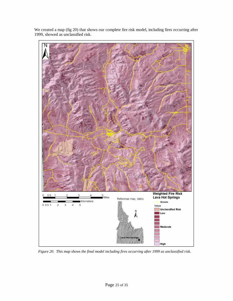
We created a map (fig 20) that shows our complete fire risk model, including fires occurring after1999, showed as unclassified risk.

Figure 20. This map shows the final model including fires occurring after 1999 as unclassified risk.

Page 26 of 35

Discussion: Early in this project we determined thresholds for no-, dry-, and moist vegetationusing NDVI. We chose the value 0.01 as a threshold between no vegetation and generalvegetation based on where and how well the NDVI values matched a DOQQ. We also visitedLava Hot Springs to observe the vegetation and insure it matched well. We chose the secondthreshold (separating dry vegetation from moisture vegetation) using similar methods. The NDVIvalue of 0.17 was the threshold limit between dry vegetation and moist vegetation. We based thison the vegetation observed in and around Lava Hot Springs. There is quite a lot of moistvegetation in that area and we believe, by reviewing the DOQQ’s, the threshold between dryvegetation and moist vegetation is best approximated at 0.17.

After estimating the different fire model components, we decided (with Keith T. Weber) howimportant each component was to the fire model, depending on how high its risk is forcommunities.

Fuel load/Rate of Spread 25% (of total fire risk model)The Fuel load/Rate of Spread component got the highest risk. This is because fast spreading firesare the most dangerous fires. It also gives the firefighters a shorter time to suppress the fire beforeit gets to the urban areas.

Fuel load/Vegetation Moisture 23%The Fuel load/Vegetation Moisture component received the second highest risk because dryvegetation with moderate fuel load are good conditions for a fire.

Fuel load/Intensity 20%The Fuel load/Intensity component also has a significant risk to communities. Thus if firefightersdo not suppress the fire, it will keep spreading.

Slope/Suppression Difficulties 17%The Slope/Suppression Difficulties component is a substantial fire hazard because if firefighterscannot reach the fire, it will keep burning although other components describe the area as lowrisk.

Slope/Rate of Spread 10%The Slope/Rate of Spread component is also a high risk for communities, but not as important asFuel load/Rate of Spread, that is why we rated it quite low.

Aspect/Sun position and Daily temperature 5%The Aspect/Sun position and Daily temperature component is rated relatively low because if afire starts on a hot day, at the end of the summer (when most of the wildfires occur), the directionthe slope is facing is less important.

When we had added together the fire model components, we realized that it did not include firesthat occurred after 1999. We added these fires to the final model and categorized the areas as“unclassified”. This is because we could no longer rely upon the fire risk model. Nor could we seta fire risk for those areas, thus we gave them the value “unclassified”.

Since much of this project is based on estimations and expert knowledge of individuals, thepurpose for it is not to be a final product. The goal for our model is to be a tool to assistfiremanagers and decision-makers. As we treated each analysis separately, we believe the resultshave accuracy adequate to fit this purpose. We further believe our model gives a good overviewof the fire risk in our study area and that it is easy to understand. Because the model is easy to

Page 27 of 35

understand, it should be applied to other users, which was a primary objective with this study.More research can be done on the different component and further development can be made onthe unclassified areas in the final WUI fire risk model.

Assessments of errors and bias: All estimations in this report are made based upon our knowledgeof the criteria. We have also discussed our analyses and results with Keith T. Weber. Except forthe fuel load/vegetation moisture model, we used the same weightings that were used during theCity of Pocatello project, (Mattsson and Thoren, 2002).

When we weighted the fuel load/vegetation moisture model by worst case scenario, wediscovered that some classes could be calculated in two ways (e.g. class 6 could be Fuel load 3 (2tons/acre)*2 (dry vegetation) and 6 (>6 tons/acre)*1 (no vegetation)). We discovered that manypixels in the grid had the latter combination (Appendix D). It is unlikely that you could have acombination of high fuel load (6) and no vegetation (1) in the grid. NDVI only recognizesvegetation with chlorophyll. This means there could be areas with a high amount of fuel, butvegetation (fuel) that is very dry. The NDVI will therefore not recognize it as vegetation.

The fuel load model had difficulties detecting juniper in some areas, but it has been validatedduring the summer (2002). Unfortunately, our WUI fire risk model used an older fuel model.Another problem with our fire risk model is that fires occurring after 1999 were not included.This resulted in “unclassified” areas in our final model, because we could not classify the fire riskin those areas.

Reference cited:Mattsson, D. and Thoren, F., 2002. Wildland/Urban Interface and Communities at RiskAmdahl, Gary, (2001). Disaster Response: GIS for Public Safety United States of America: ESRIPRESS.

Acknowledgements:On July 29, 2002 we had a presentation of our project for people that have good knowledge aboutthis subject. We discussed the weightings of the wildfire model components and accepted theweightings described in this report.

These people were attending:Felicia Burkhardt, GIS Coordinator, USRD BLMFred Judd, Fire Mitigation and Education Officer, USDR BLMDon Gosswiller, Fire Mitigation and Education Officer, USDR BLMKeith T. Weber, GIS Director, Idaho State University (ISU), GIS Training and Research Center(GISTReC)Cecilia Jansson, GIS Intern, ISU, GISTReCOskar Pettersson, GIS Intern, ISU, GISTReC

Page 28 of 35

Appendix A – Cartographic Model

Cartographic Model

Page 29 of 35

Description

1 We converted the DEM quadrangles to DEM-lattice in ArcInfo Workstation2 We merged the DEM lattices together with ArcInfos mosaic3 By using the footprint of the merged grid, we created a “cookie cutter” with gridclip4 We converted the image to grid with ArcInfos imagegrid5 By using the cookiecutter, we clipped the fuelmodel6 By using the cookiecutter, we clipped the streets7 By using the cookiecutter, we clipped the vegetation8 We reclassed the vegetation by using Spatial Analyst’s reclassify9 We converted the image to grid with ArcInfos imagegrid10 By using the cookiecutter, we clipped the Emergency Response Time Model11 We converted the satellite band images to grids with ArcInfos imagegrid12 To make the grids able to handle decimals, we used the ArcInfos float13 In grid we made aoc_ndvi = (f_satb4 - f_satb3) / (f_satb4 + f_satb3)14 By using the cookiecutter, we clipped the ndvi to our area of concern15 In raster calculator we made classes for everything > 0, 0.05, 0.1, 0.15, 0.2, 0.25 and 0.3,

then we compared these with aoi_lavaveg16 We multiplied aoi_lavavegrc and the ndvi classes to see if the ndvi classes says it is

vegetation where aoi_lavavegrc says it is paved urban17 We made three new classes of the ndvi, no veg, dry veg and moist veg18 We multiplied aoi_vegmod with aoi_lavafuel19 We made a hillshade to make it easier when we compare different grids20 We made a slope from aoi_lavadem in Spatial Analyst à surface analysis à slope21 We reclassed the slope grid to the “suppression difficulties” values22 We reclassed the slope again but to the “rate of spread” values23 From aoi_lavadem we made an aspect in Spatial Analyst à surface analysis à aspect24 We reclassed the aspect to the “aspect/sun position and daily temperature” values25 We reclassed the aoi_fuelmodel to the “rate of spread” values26 We reclassed the aoi_fuelmodel again but to the “fire intensity” values27 From aoi_lavastreet and lava fire dept (position of fire station), we made lava_response

in Network Analyst - service area28 We converted lava_response to a grid29 We weighted the hole lava_response with 10 and got response_time30 We weighted the ndvi_fuelmodel which resulted in aoi_fuelveg31 We merged aoi_lavaros, aoi_lavasup, aoi_lavaasprc, aoi_fuelros, aoi_fuelintco, and

aoi_fuelveg by adding them together

Page 30 of 35

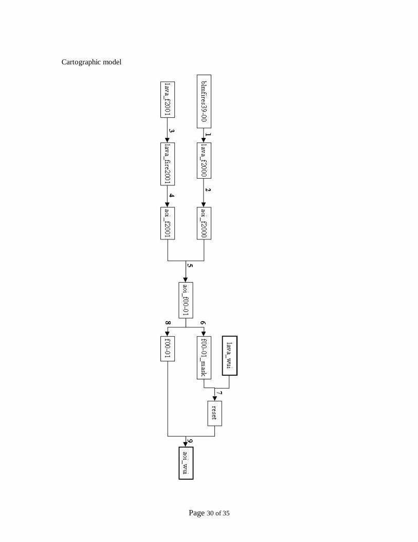
Cartographic model

Page 31 of 35

Description

1 We selected all fires from 2000 and then we converted them to a grid2 We clipped lava_f2000 with the cookiecutter in gridclip3 We selected the fire within our area of interest4 We converted feature to grid5 We merged aoi_f200 and aoi_f2001 together by adding them (No Data=0 in both)6 We reclassed aoi_f00-01 (class 1=0, class 2=0, No Data=1)7 With arithmetic, we multiplied lava_wui and f00-01_mask8 We reclassed aoi_f00-01 (class 1=1, class 2=1, No Data=0)9 With arithmetic, we multiplied F00-01 and reset, and we have our final product.

Page 32 of 35

Appendix B – Weightings

These tables show the weightings we used to weight our fire risk model components.

Table 6. Weighting data for Fuel load/ Table 7. Weighting data for FuelVegetation Moisture. Compare with load/Rate of Spread. Compare withfigure 2 in report. figure 3 in report.

Table 8. Weighting data for Fuel Table 9. Weighting data for Slope/Rate ofload/Intensity. Compare with figure Spread. Compare with figure 5 in report.4 in report.

Page 33 of 35

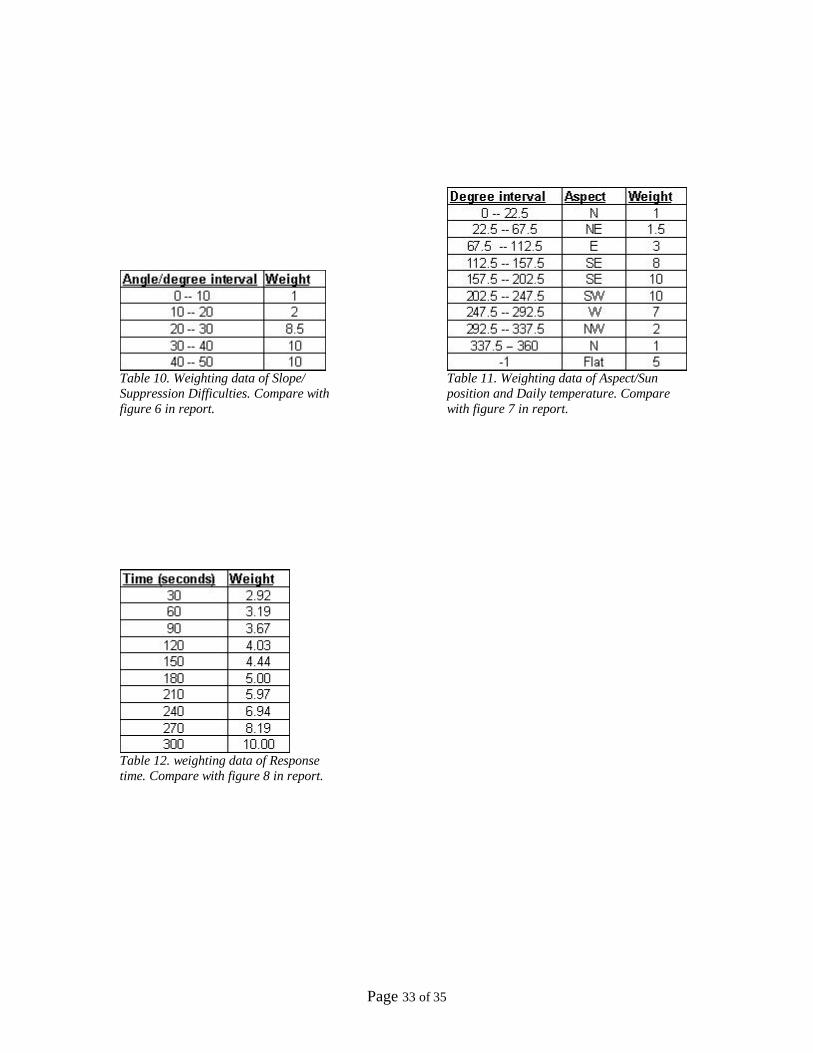
Table 10. Weighting data of Slope/ Table 11. Weighting data of Aspect/SunSuppression Difficulties. Compare with position and Daily temperature. Comparefigure 6 in report. with figure 7 in report.

Table 12. weighting data of Responsetime. Compare with figure 8 in report.

Page 34 of 35

Appendix C – Data dictionary

Page 35 of 35

Appendix D – Errors in the worst criteria scenario

This figure shows the different ways to calculate the fuel load/vegetation moisture classes. Thefuel load/vegetation moisture model is the result of vegmodel (NDVI-based grid) and lavafuel(fuel load model) multiplied together. It also shows how many pixels each way of calculationhave in the grid.