Prof. Hui Jiang Department of Computer Science and Engineering York University, Toronto, Ont. M3J 1P3, CANADA

Why DNN Works for Acoustic Modeling in Speech

Recognition?

Joint work with Y. Bao, J. Pan, O. Abdel-Hamid

Outline •  Introduction

• DNN/HMM for Speech

• Bottleneck Features

•  Incoherent Training

• Conclusions

• Other DNN Projects This talk is based on the following two papers: [1] J. Pan, C. Liu, Z. Wang, Y. Hu and H. Jiang, ``Investigations of Deep Neural Networks for Large Vocabulary Continuous Speech Recognition", Proc. of International Symposium on Chinese Spoken Language Processing (ISCSLP'2012), Hong Kong, December 2012. [2] Y. Bao, H. Jiang, L. Dai, C. Liu, “Incoherent Training of Deep Neural Networks to De-correlated Bottleneck Features for Speech Recognition," submitted to 2013 IEEE International Conference on Acoustics, Speech, and Signal Processing (ICASSP'13), Vancouver, Canada.

Introduction: ASR History • ASR formulation:

o GMM/HMM + n-gram + Viterbi search

•  Technical advances (incremental) over past 10 years: o Adaptation (speaker/environment): 5% rel. gain o Discriminative Training: 5-10% rel. gain o  Feature normalization: 5% rel. gain o ROVER: 5% rel. gain

• More and more data better and better accuracy o  read speech (>90%), telephony speech (>70%) o meeting/voicemail recording (<60%)

Acoustic Modeling: Optimization • Acoustic modeling large-scale optimization

o  2000+ hour data GMMs/HMM billions of samples 100+ million free parameters •  Training Methods

o Maximum Likelihood Estimation (MLE) o Discriminative Training (DT)

• Engineering Issues o Efficiency: feasible with 100-1000 of CPUs o Reliability: robust estimation of all parameters

Neural Network for ASR •  1990s: MLP for ASR (Bourlard and Morgan, 1994)

o NN/HMM hybrid model (worse than GMM/HMM)

•  2000s: TANDEM (Hermansky, Ellis, et al., 2000) o  Use MLP as Feature Extraction (5-10% rel. gain)

•  2006: DNN for small tasks (Hinton et al., 2006) o RBM-based pre-training for DNN

•  2010: DNN for small-scale ASR (Mohamed, Yi, et al. 2010)

•  2011: DNN for large-scale ASR o Over 30% rel. gain in Switchboard (Seide et al., 2011)

ASR Frontend

Feature Extraction (Linear Prediction, Filter Bank)

waveform

Feature vectors

sliding window

Audio Segmentation Speech Recognition

speech/music/noise words

Audio/speech coding

bit stream for transmission

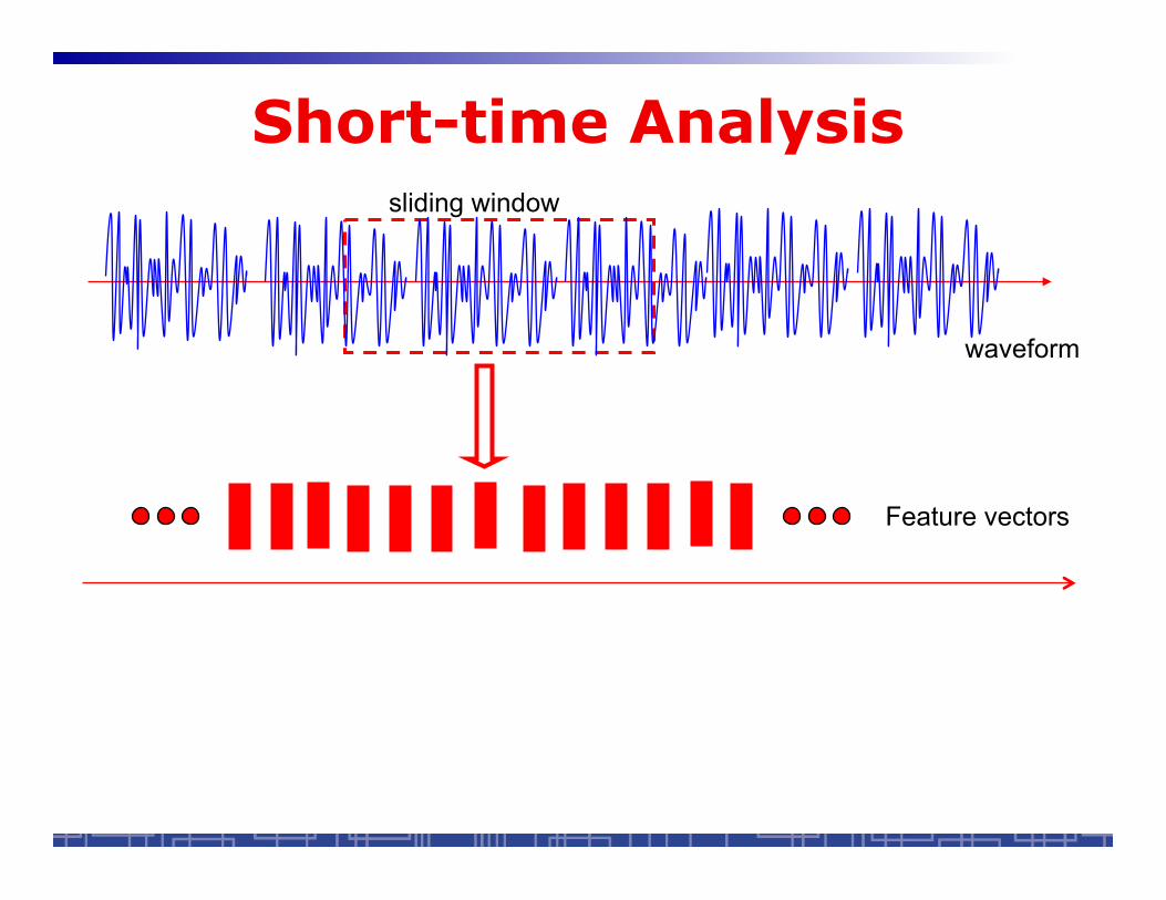
Short-time Analysis

waveform

Feature vectors

sliding window

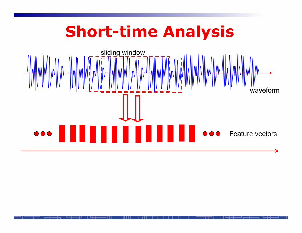
Short-time Analysis

waveform

Feature vectors

sliding window

Short-time Analysis

waveform

Feature vectors

sliding window

Short-time Analysis

waveform

Feature vectors

sliding window

ASR Frontend: GMM/HMM

waveform

Feature vectors

sliding window

ASR Frontend: NN/HMM

waveform

Feature vectors

sliding window

…

…

NN for ASR: old and new • Deeper network

more hidden layers ( 1 6-7 layers)

• Wider network

More hidden nodes More output nodes (100 5-10 K )

• More data 10-20 hours 2-10 k hours training data

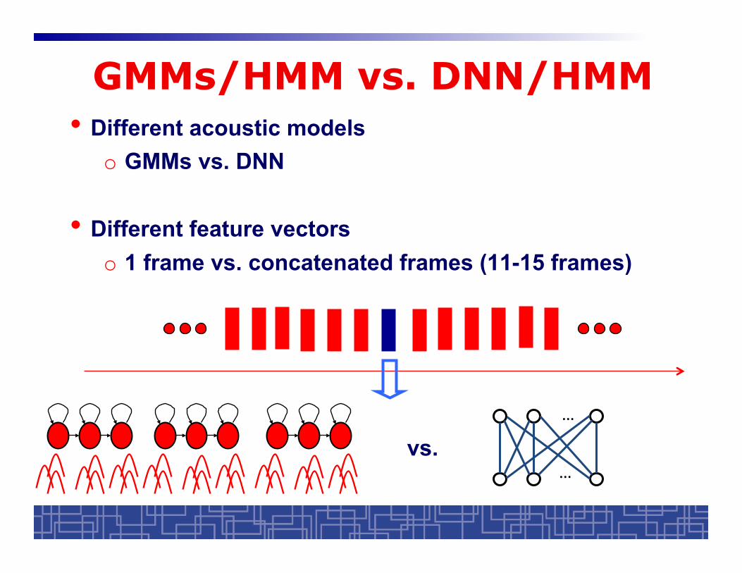
GMMs/HMM vs. DNN/HMM • Different acoustic models

o GMMs vs. DNN

• Different feature vectors o  1 frame vs. concatenated frames (11-15 frames)

vs. …

…

Experiment (I): GMMs/HMM vs. DNN/HMM

•  70-hour Chinese ASR task; 4000 tied HMM states • GMM: 30 Gaussians per state • DNN: pre-trained; 1024 nodes per layer; 1-6 hidden layers

Numbers in word error rates (%) NN-1: 1 hidden layer; DNN-6: 6 hidden layers MPE GMM: discriminatively trained GMM/HMM

Experiment (II): GMMs/HMM vs. DNN/HMM

•  320-hour English Switchboard task; 9000 tied HMM states • GMM: 40 Gaussian per state • DNN: pre-trained; 2000 nodes per layer; 1-5 hidden layers Numbers in word error rates (%)

NN-1: 1 hidden layer; DNN-3/5: 3/5 hidden layers MPE GMM: discriminatively trained GMM/HMM

Conclusions (I) •  The gain of DNN/HMM hybrid is almost entirely attributed

to the concatenated frames.

o  The concatenated features contain almost all additional information resulting in the gain.

o But they are highly correlated.

• DNN is powerful to leverage highly correlated features.

What’s next • How about GMM/HMM?

• Hard to explore highly correlated features in GMMs. o Requires dimensional reduction for de-correlation.

•  Linear dimensional reduction (PCA, LDA, KLT, …) o  Failed to compete with DNN.

• Nonlinear dimensional reduction o Using NN/DNN (Hinton et al.), a.k.a. bottleneck features o Manifold learning, LLE, MDS, SNE, …?

Bottleneck (BN) Feature

Experiment (I): Bottleneck(BN) Features

70-hour Chinese ASR Task (word error rate in %) MLE: maximum likelihood estimation

MPE: discriminative training

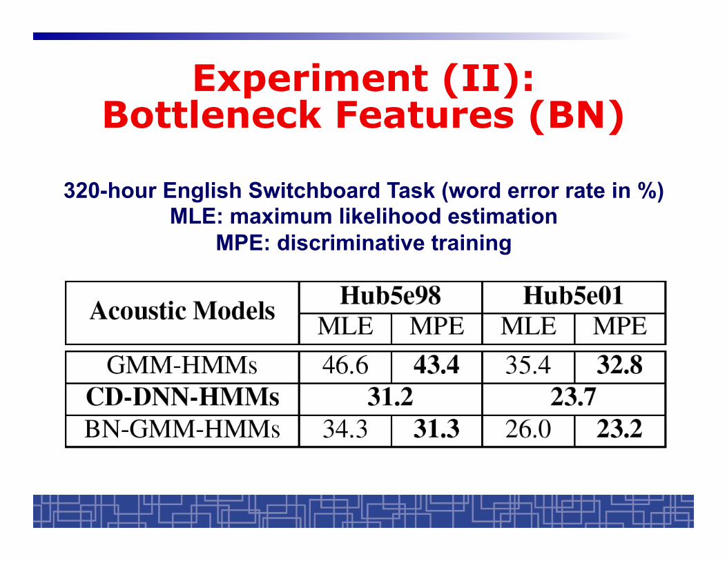
Experiment (II): Bottleneck Features (BN)

320-hour English Switchboard Task (word error rate in %) MLE: maximum likelihood estimation

MPE: discriminative training

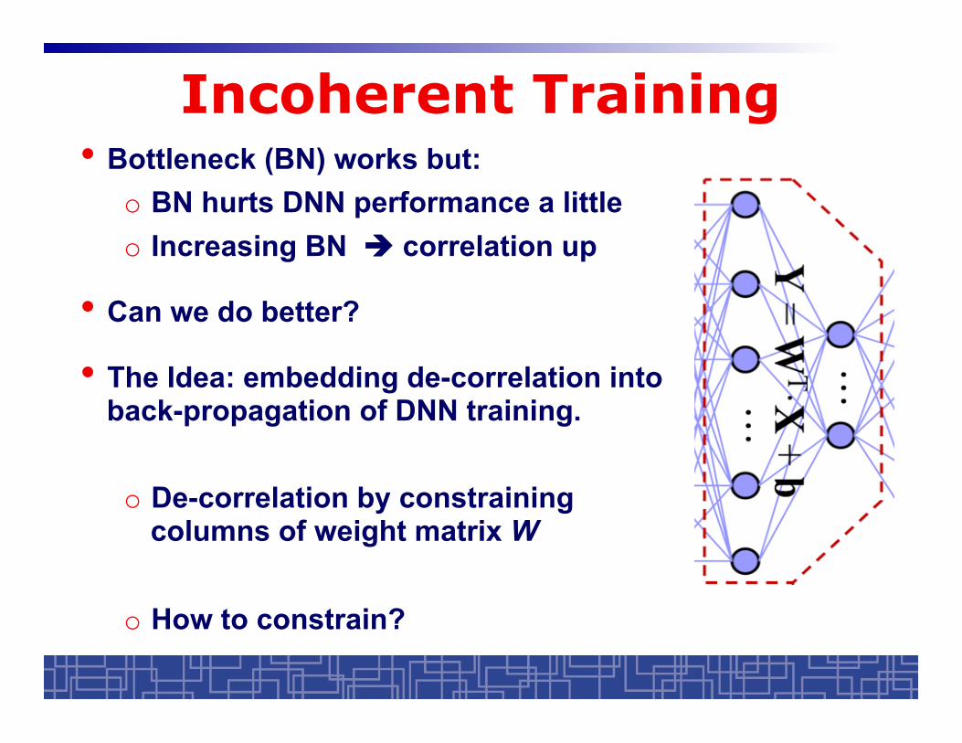
Incoherent Training • Bottleneck (BN) works but:

o BN hurts DNN performance a little o  Increasing BN correlation up

• Can we do better?

•  The Idea: embedding de-correlation into back-propagation of DNN training.

o De-correlation by constraining columns of weight matrix W

o How to constrain?

Incoherent Training • Define coherence of DNN weight matrix W as:

• A matrix with smaller coherence indicates all of its

column vectors are less similar.

• Approximate coherence using soft-max:

GW =maxi, j

gij =maxi, j

wi ⋅wj

wi wj

GW

Incoherent Training • All DNN weight matrices are optimized by minimizing a

regularized objective function:

• Derivatives of coherence:

• Back-propagation is still applicable…

F (new) = F (old ) +α ⋅maxW

GW

∂GW

∂wk

Incoherent Training: De-correlation

Applying incoherent training to one weight matrix in BN

Incoherent Training: Data-driven

•  If only applying to one weight matrix W:

• Covariance matrix of Y:

• Directly measure correlation coefficients based on the above covariance matrix:

with Cx is estimate from one mini-batch each time

GW =maxi, j

gij

Y =WTX + b

CY =WTCXW

Incoherent Training: Data-driven

• After soft-max, Derivatives can be computed as:

where • Back-propagation still applies except Cx is computed

for each mini-batch

∂GW

∂wk

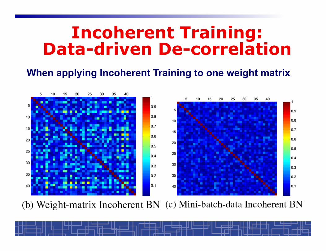
Incoherent Training: Data-driven De-correlation

When applying Incoherent Training to one weight matrix

Experiment (I): Incoherent Training

70-hour Chinese ASR Task (word error rate in %) MLE: maximum likelihood estimation

MPE: discriminative training DNN-HMM: 13.1%

Experiment (II): Incoherent Training

320-hour English Switchboard Task (word error rate in %) MLE: maximum likelihood estimation

MPE: discriminative training DNN-HMM: 31.2% (Hub5e98) and 23.7% (Hub5e01)

Conclusions (II) • Possible to compete with DNN under the

traditional GMMs/HMM framework.

• Promising to use bottleneck features learned from the proposed incoherent training.

• Benefits over DNN/HMM: o Slightly better performance o Enjoy other ASR techniques (adaptation, …) o Faster training process o Faster decoding process

Future works • Apply incoherent training to general DNN

learning

• Other nonlinear dimensional reduction methods for concatenated features