Who Works Where and Why? Parental Networks andthe Labor Market

Shmuel San∗

August 22, 2021

Click here for the latest version

Abstract

Relying on identifying variation from the timing of job movements of parents’ coworkers,I find that workers in Israel are three to four times more likely to find employmentin firms where their parents have professional connections than in otherwise similarfirms. I use the same variation to structurally estimate a two-sided matching modelwith search frictions and find that connections double the probability of meeting andincrease by 35% the likelihood of being hired after meeting. The estimated willingnessto pay for one additional meeting with a connected firm is 3.7% of the average wage.Connections matter for inequality; the wage gap between Arabs and Jews decreases by12% when equalizing the groups’ connections but increases by 56% when prohibitingthe hiring of connected workers. These seemingly opposing results are explained by thefact that Arabs have connections to lower-paying firms but use their connections moreextensively.

JEL codes: J31, J64

∗Department of Economics, The Hebrew University of Jerusalem, Jerusalem 91905, Israel. Email:muly.san@mail.huji.ac.il. Special thanks to my advisors, Christopher Flinn, Alfred Galichon, Petra Moser,and Martin Rotemberg, for guidance and support. For their helpful comments, I thank Milena Almagro, ZlilAloni, Jaime Arellano-Bover, Barbara Biasi, Pierre-André Chiappori, Tim Christensen, Christopher Conlon,Michael Gilraine, Walker Hanlon, Elena Manresa, Konrad Menzel, Maor Milgrom, Tzachi Raz, BernardSalanié, Sharon Traiberman, Miguel Uribe, and Daniel Waldinger and audiences at SOLE 2020, NEUDC2020, EGSC 2020, Econometric Society European Winter Meeting 2020, ZEW 2021, RES 2021, NYU, He-brew University, Bar Ilan University, Tel Aviv University, Florida State University, Ben-Gurion University,Haifa University, Collegio Carlo Alberto, IDC Herzliya, University of Oslo, and IIES Stockholm.

1

1 Introduction

That some firms pay workers with similar skills differently is well documented (Abowdet al. 1999; Mortensen 2003; Card et al. 2018). Much less is known about why some workersfind higher-paying jobs than their comparable peers. As many, if not most, jobs are obtainedthrough social contacts (Topa 2011), a natural answer to this question concerns differencesin social networks.1 This article studies the role of social connections in explaining wherepeople find their first job. I focus on one particular mechanism: firms where workers haveconnections through their parents.

This question has important implications for inequality. Differences in the quality oflabor-market ties can partly explain pay gaps between groups. This paper focuses on Israel,where there is a big pay gap between the two major ethnic groups, Jews and Arabs. Usinga matched employer-employee dataset linked to the Israeli population registry, I show thatArabs have parental connections to lower-paying firms, and I study the importance of thatmechanism in explaining the pay gap.

I distinguish between strong and weak parental connections. Strong (direct) connectionsare connections between employees and firms where their parents have worked. Weak (indi-rect) connections are between employees and firms where their parents’ past coworkers haveworked. The first part of the paper studies the reduced-form relationship between parentalconnections and first-job assignments as well as wages. My main focus is understanding theimpact of weak connections on a worker’s first job.

To identify the effect of weak connections, I leverage the timing of both the formationand destruction of links. In particular, I compare the likelihood of working in a firm wherethe employee had active links in the labor-market entry year ("weak connections") with thelikelihood of working in a firm where the contact had left a short time before or had joineda short time afterward ("phantom connections"). I show that firms with weak and phantomconnections are similar on a variety of characteristics such as sector and location.

I find that workers are 3.7 times more likely to find employment in firms with (real) weakparental connections than in phantom-connected firms. Workers’ probability of starting ata particular firm discretely falls the year after the link is destroyed.

To check for the possibility that estimated effects reflect endogenous separations, I esti-mate the effects using two exogenous causes of separation; coworkers’ deaths and retirements.Specifically, I compare the probability of working at firms in which parents’ coworkers diedor retired after the labor-market entry year and firms in which contacts died or retired a few

145% of the workers in 2016 in Israel reported they found their job through social connections (CBS2018).

2

years before.2 These estimates are similar in magnitude to the benchmark result, with oddsratios of 2.6 and 3.9 for the "death" and "retirement" connections, respectively. Likewise,to check the potential difference in employment trends in firms with weak and phantomconnections, I perform a placebo test, assigning a worker’s connections to a random workerwith similar observable characteristics. I find no hiring differences between phantom andreal connections of a placebo worker.

Connections are more effective if formed at smaller firms, for more extended periods,and more recently. Notably, connections are also stronger if the child, parent, and parent’scoworker share characteristics such as gender or ethnicity.3 Likewise, the effect is strongerfor males, Arabs, and less-educated workers.

I end the first part of the paper by studying the relationship between social connectionand pay. Weak connections are associated with 1.4 percent higher wages than phantomconnections. However, this analysis does not identify the causal effect of social connectionson wages since it ignores selection: without connections, a hired connected worker may havecounterfactually not received an offer at all instead of a different salary.4

To addresses this issue, together with other limitations of the reduced-form estimation,5

I develop and estimate a two-sided matching model of the labor market with search frictionsin the second part of the paper. The model addresses the selection problem by jointlystudying questions of matching and wage-setting. The model also helps to understand theexact ways social connections can be valuable for matching workers and firms. I focus ontwo mechanisms. First, social connections might alleviate search frictions by improving theinformation flow about a job opening at a specific firm and a potential job seeker. Second,conditional on that mutual knowledge, they may increase the probability of a match betweenthe job seeker and the firm.6

In particular, the model assumes that matching takes place in two stages. In the firststage, workers and firms meet randomly, and the probability of meeting can vary as a functionof connections. In the second stage, workers and firms that have met choose their optimal(stable) match based on the utility they obtain from the match, which also might be affected

2See Azoulay et al. (2010) and Jager (2016) for early use of death for exogenous variation in networks.3That is to say, for example, that fathers’ connections matter more for boys and mothers’ for girls.4Unlike the matching question where the outcome (working or not) is observed for each worker-firm

combination, the outcome of the wage-setting question is only observed if the firm hires the worker.5The reduced-form estimation abstracts from spillovers and equilibrium effects. The model addresses

it by considering the full structure of connections in the economy in an equilibrium framework. See thebeginning of section 5 for more details.

6Differentiating between these two mechanisms is essential for predicting the effectiveness of differentpolicy measures. For example, if the second mechanism is the one that matters, then merely encouragingjob interviews is unlikely to have a sizable impact. In contrast, other policies, such as subsidizing long-terminternships, are likely to have an impact through both mechanisms.

3

by social connections. To separately identify the two mechanisms, I use two distinct typesof information: where individuals end up working and how much they are paid.

I estimate the model using a simulation-based method that allows for rich and flexiblevalue functions. Finding the model’s equilibrium matches and wages is computationallyfeasible due to the sparsity of the data resulting from the model’s first stage, which restrictsthe set of potential matches. I estimate the parameters of the model using a novel updatemapping that "inverts" the information on the observed matches and wages into the meetingprobability and match-surplus parameters.

The model estimates suggest that both the "search frictions" and "match surplus" mech-anisms are important in explaining why parental connections increase the probability ofworking in a firm. Weak connections increase the meeting probability by 115% and thelikelihood of being hired given a meeting by 35%.

To study the wage effects of connections using the model, I evaluate two sets of coun-terfactuals. Both counterfactuals rely on the assumption that connections’ causal impactis the excess effect of real connections relative to phantom connections. In the first set ofcounterfactuals, I evaluate the wage-equivalent value of meetings and connections. I findthat the average value of one additional meeting with an unconnected firm is 2.2% of newworkers’ average wages. On the other hand, isolating only the match quality mechanism byadding a causal weak connection to a random existing meeting increases the wage by 1.5%the average wage. Combining the two mechanisms, the value of a new meeting with causalweak connections is 3.7% of the average wage. 84% of this effect is due to workers movingto the new connected firm, whereas the remaining 16% is due to improving workers’ choiceset without changing their job.

My model also allows me to evaluate the impact of parental connections on between-group wage inequality. Specifically, in the second set of counterfactual exercises, I checkhow much of the pay gap between Jews and Arabs in Israel is due to Jews having parentalconnections to higher-paying firms. I find that if Arabs and Jews had the same quantity andquality of connections, the ethnic wage gap would decrease by 12% compared with the actualgap. However, when prohibiting the hiring of connected workers, the ethnic pay gap wouldincrease by 56%. Two opposing forces are at play in these two scenarios. On the one hand,Arabs have connections to lower-paying firms than Jews. Therefore, equalizing connectionsprovides Arabs with better connections, which reduces the pay gap. On the other hand,Arabs rely more heavily on connections. Prohibiting the use of connections increases thegap as it hurts Arabs more than Jews.

I make five contributions in this paper. First, I offer a new identification strategy forthe effect of indirect parental connections on labor market outcomes. Studying the entire

4

network of parents’ coworkers provides more variation than looking only at parents’ employ-ment. Moreover, the assumption that the timing of job movements of parents’ colleaguesis orthogonal to the workers’ labor market entry makes much less sense if applied to theparents themselves.

Second, I develop and estimate a model that combines the two types of mechanismsusually studied in isolation in the literature regarding the impact of social connections onlabor market outcomes: search frictions and match surplus. To the best of my knowledge,this is the first work that studies these mechanisms in a joint framework. I combine theidentifying variation studied in the first part of the paper with the asymmetry relationshipsbetween the moments and the parameters implied by the model to separately identify thecausal impact of social connections through the two different mechanisms.7

Third, I contribute to the two-sided matching literature by introducing search frictionsinto this type of model. I exploit the assignment problem’s sparsity implied by the search-frictions assumption, together with recent developments in assignment problem algorithms,to simulate the model. Thus, I can perform a simulation-based estimation of the model withlarge-scale data, which allows for potentially rich and flexible utility functions.8

Fourth, I suggest a novel estimation procedure to estimate two sets of unobserved modelcharacteristics with two sets of data points. In each iteration, the parameters are updatedone by one to the direction that best fits the data.9 This directed updating procedure enablesestimating models with many parameters, even when the simulation of each model’s iterationis expensive. Taken together, the model proposed in this paper can serve as a workhorse forstudying various questions regarding the labor market.

Fifth, I use the model to study the impact of differences in the quality of connectionspeople inherit from their parents on between-group inequality. By that, I show that socialconnections are not only important for individuals but also matter for the society at large,particularly for income inequality.

Existing literature studying parental connections finds that direct links (where parentswork) increase the child’s probability of working there; however, there is less evidence for theimpact of indirect parental connections (Corak and Piraino 2011; Kramarz and Skans 2014;

7In the model, the group’s match surplus significantly impacts both the groups’ number of matches andwages. In contrast, the group’s meeting rate has a significant impact on the number of matches but (almost)no impact on wages.

8For example, the model relaxes the "separability assumption" which is in use in the majority of thisliterature (Salanié 2015; Chiappori et al. 2017; Galichon and Salanié 2020). However, see Fox et al. (2018)for a notable exception. See also Agarwal (2015) for a simulation-based estimation of a non-transferableutility model of the market for medical residents.

9This estimation procedure extends the contraction mapping algorithm proposed by Berry et al. (1995)to "invert" one set of data points into one set of parameters.

5

Plug et al. 2018; Staiger 2021). The positive effect I find for the channel of parent’s pastcoworkers’ network compared to other channels of indirect networks (e.g., parents of high-school classmates or high-school classmates of one’s parents) is consistent with a literatureshowing the importance of coworker networks for labor market outcomes (Granovetter 1973;Cingano and Rosolia 2012; Hensvik and Skans 2016; Caldwell and Harmon 2019).10

As mentioned earlier, the theoretical literature offers two main mechanisms for the impor-tance of social connections for matching workers and firms. First, social connections mightimprove the information flow about job opportunities and job seekers (Calvo-Armengol andJackson 2004; Fontaine 2008). Second, connections might impact the value of the prospec-tive match, which may be due to an impact on the productivity of the match (Athey etal. 2000; Bandiera et al. 2009), favoritism (Beaman and Magruder 2012; Dickinson et al.2018), or to reducing uncertainty about the productivity of the worker or the match (Mont-gomery 1991; Dustmann et al. 2016; Bolte et al. 2020). In this paper, I build and estimatea matching model that separately identifies these two mechanisms. Part of this literaturealso emphasizes the theoretical link between social connections and between-group inequality(Calvo-Armengol and Jackson 2004; Bolte et al. 2020). I use estimates from my model toempirically study this link in the context of the ethnic pay gap in Israel.

Finally, this paper introduces search frictions into a two-sided matching model (Choo andSiow 2006; Chiappori and Salanié 2016). This extension empowers the model to study labormarkets where search frictions are important (Mortensen and Pissarides 1994; Postel–Vinayand Robin 2002).11

2 Data

I use matched employer-employee administrative records from Israel. These data span1983-2015 and contain administrative information about the entire Israeli workforce collectedfrom tax records. The dataset includes person identifiers, firm identifiers, monthly indicatorsfor each firm in which a person worked, the yearly salary received from each employer in ayear, and the firms’ industry.12

The employment tax records are merged with the Israeli Population Registry. This10I also find that the effect of connections decays over time, which explains why links formed a long time

ago are not useful.11See Jaffe and Weber (2019) for an earlier theoretical study introduces differential meeting rates into

Choo and Siow (2006)’s matching model. See Del Boca and Flinn (2014) for a matching model (of themarriage market) with restricted choice sets. Finally, see Caldwell and Danieli (2021) for a recent study thatuses a two-sided matching model to derive a sufficient statistic for studying the effect of outside options onwages.

12The data do not include establishment/plant identifiers or an indicator for multi-plant firms.

6

dataset covers the full population of Israel. It includes demographic information: date ofbirth, date of death (if any), sex, ethnic group, country of birth, and date of immigrationto Israel. Most important for this study, the data include identifiers of the parents of eachindividual, which enables me to link parents and children. Finally, starting in 2000, I observeyearly geocoded information on the city of residence for each individual.

I also use data on higher-education enrollment of the individuals collected by the NationalInsurance Institute. Starting in 1996, I observe the higher-education institution and periodof enrollment of each individual in Israel.

2.1 Sample selection

I construct a panel dataset at the annual frequency. Following Kramarz and Skans (2014),I assign each person-year observation the firm in which that person was employed duringFebruary. I calculate the monthly salary by dividing the yearly salary in a firm by the numberof months worked there. If someone worked at more than one firm during February, I assignhim or her to the firm that paid a higher monthly salary. I exclude from the sample worker-year observations with less than 25% of the national average monthly wage.13 The period ofthe sample is 1991–2015. I construct a second dataset from this panel dataset, keeping onlyfirms with 5-500 workers each year. I use these data to build a parental network over time.14

My analysis sample comprises Israelis who found their first stable job (see definitionbelow) between ages 22-27 in the years 2006-2015 in a 5-500 workers firm. I exclude workerswithout any parent that worked in a 5-500 workers firm when they were 12-21 years old. Ifurther exclude immigrants and Ultraorthodox Jews from the sample.15

13The minimum monthly salary in 2015 was 48.8% of the average salary in that year. This ratio fluctuatedbetween 40%-50% in 1990-2015. Therefore, I exclude workers who earn approximately 50% or less theminimum wage, similarly to Kramarz and Skans (2014). See Appendix B for further details on the datacleaning.

14Intuitively, the probability that a random pair of workers form social connections decreases in the firm’ssize. Below, I show that, indeed, the effect of having a parental connection in a firm on the probability ofworking at that firm decreases when the firm’s size increases. Moreover, I show that the effect disappearsfor firms with more than 400 workers. Therefore, assuming that a pair of workers in large firms havesocial connections would increase the error in the measurement of connections and could downward-bias theestimates of the effect of connections. In 2006-2015, 392 unique firms in Israel employed more than 500workers (0.2% of the firms). Those firms employ, on average, 37.6% of the yearly labor force. Firms with1-4 workers account for 70.2% of the firms in that period but employed only 10.2% of the labor force. Firmswith 5-500 workers, for which this paper studies the effect of social connections, account for 29.6% of thefirms in 2006-2015, and employed 52.2% of the labor force (Table A1).

15Usually, immigrants do not have parental connections in the labor market. See Arellano-Bover andSan (2020) for the role firms play in explaining the pay gaps between former Soviet Union immigrantsand natives in Israel. Ultraorthodox Jews in Israel have unique labor-market characteristics, such as low(secular) education and employment rates, especially for males (Berman 2000; Fuchs and Epstein 2019).Specific research is needed to study this group.

7

2.2 Definition of first stable job and labor-market entry year

This paper focuses on the employment and salary of young people when they enter thelabor market. It does it for two reasons. First, young workers’ first job experiences areimportant for their future careers (Oreopoulos et al. 2012; Arellano-Bover 2020). Second,focusing on first-job outcomes enables isolating the impact of the initial set of connectionsthe workers enter the labor market with—parental professional network in this case—fromthe connections the worker herself forms at the labor market (and might be impacted by theinitial connections as well).

Following Kramarz and Skans (2014), I define the first stable job as the first job afterhigher-education graduation (if applicable) that lasts for at least four months during a cal-endar year and produces total annual earnings corresponding to at least 150% the nationalaverage monthly wage. Labor-market entry year is the year the new worker finds her firstjob.16

2.3 Definition of parental connections

The focus of this study is on the professional network of parents. I study two types ofparental professional connections: weak and strong.

Weak connections are connections between workers and firms in which precisely one oftheir parent’s past coworkers currently works. Specifically, a worker i is (weakly) connectedto a firm j if i’s parent and a worker k worked simultaneously at the same firm when i was12-21 years old, and k worked at a firm j at i’s labor-market entry year. Both past andcurrent firms employ between 5 and 500 employees.

Strong connections between a worker i and a firm j satisfy at least one of the followingconditions: 1) i’s parent worked at a firm j when i was 12-21 years old, 2) more than one ofi’s parent’s past coworkers worked at a firm j at any time within five years before or afteri’s labor market entry year.

16I do not distinguish between the year the fresh graduate looks for her first job and the year she findsher first job. Observing unemployment before starting the first job is difficult in administrative data as onlypreviously employed workers are eligible for unemployment benefits. Potentially, I could use the assignmentof workers at some fixed age or a fixed number of years after graduation and define people without a jobat that time as unemployed. I choose not to do this for two reasons. First, it is challenging to differentiatepeople who unsuccessfully looked for a job from those who did not look for a job based on employmentinformation alone. For example, many Israeli youths postpone their entry into the labor market becausethey take a long backpacking trip following military service (Noy and Cohen 2005). Second, using the job ata fixed age might bias the estimates of the effect of connections. For example, if the worker starts workingat the firm before that age and the contact left the firm right after she starts working there, I might definethat firm as a firm with phantom connections (see definition below) even though the worker had activeconnections there when she joined the firm.

8

Two components of these definitions are noteworthy. First, to reduce the "endogeneity"in measuring connections, I define the parent’s past firms and past coworkers using a fixedperiod of time (the child is 12-21 years old). I do not include connections formed at theyears between the child is 22 until the year she enters the labor market. Doing so wouldmechanically increase the set of connections available for workers that enter the labor marketlater.

Second, I assign worker-firm pairs with more than one past parental coworker to thegroup of strong connections for three reasons. One, it allows me to use the single coworker’scharacteristics for the classification of the connections. For example, I later define weak andphantom connections by the years the coworker worked at the firm. Likewise, the "death"and "retirement" connections are based on coworker’s demographic characteristics. It isunclear how to define those concepts when there is more than one contact in the firm. Two,when many parental coworkers work at the same firm, it might be the case that this firm issome continuation of the parent’s past firm, e.g., a firm that merged or acquired the parentfirm or merely the same firm with a different identifier. Grouping together firms with manyparental coworkers and parents’ past firms eliminates weak connections estimates’ upwardbias. Three, keeping both weak and phantom connections with only one contact makes themcomparable. It therefore provides a more accurate estimate for the main effect of interest,namely the effect of weak (indirect) connections. However, I also check the robustness of theresults for different definitions of connections (see Table A3).

2.4 Workers’ and Firms’ characteristics

The paper’s empirical analysis compares the firm assignment and wages of new workerswith similar observable characteristics. These characteristics include age, gender (male/fe-male), education (no college/college), ethnicity (Jew/Arab), and district of residence.

Firms’ characteristics include the industry, location, and firm pay premium for each firm.I use the 3-digit industry code of each firm (2011 Israeli classification). The firms’ locationsare determined by the median longitude and latitude of the workers’ city of residence. Thefirm pay premiums are estimated using the AKM model (Abowd et al. 1999). These pre-miums aim to capture the average differences in salary firms pay to similar workers.17 SeeAppendix B for further information about the definitions of the variables.

17The firm premiums are not necessarily a proxy for the productivity of the firms but might captureother factors that lead to differences in salary, such as differential rent sharing. See Card et al. (2018) for adiscussion of the AKM model and the critique of it. In this paper’s model, I use the AKM firm premiumsonly to classify firms into bins. The model’s "pay premium" of each bin of firms is estimated within themodel and not based on the AKM premiums.

9

2.5 Summary statistics

Table 1 shows sample sizes and sample means. The new workers’ sample—my mainanalysis sample—includes 220,877 workers, of which 29% are Arabs, 43% are female, and23% have some college education. The average age at first stable employment is 24, and theaverage monthly salary is 5,836 NIS, which is equivalent to 1,621 USD (2017 prices).

On average, Jews who enter the labor market earn more at their first job and work atbetter firms (in terms of pay premiums) than Arabs. Additionally, Jews are connected tohigher-paying firms via both strong and weak connections. However, the share of workerswho find their first job in a connected firm is higher for Arabs than for Jews (Table 1).

Comparing males and females, males earn more at their first job but work at similar-paying firms to females. Likewise, males are connected to firms with slightly lower rank (interms of pay premium) than females. Finally, the share of workers who find their first jobin a connected firm is higher for males than for females.

To better understand the distribution of connections, I group the firms into five binsusing the pay premiums. Figure 1 shows the number of weak and strong connections withineach bin of firms for different groups of workers. Panels A and B show that, on average,Jews and Arabs have the same number of connections with firms at the lowest quintile ofpay premiums. However, Jews have more connections with higher-ranked firms than Arabs,and the gap increases as the firm’s rank increases. Overall, the quality of connections (interms of the pay premium of the connected firms) is better for Jews than Arabs.

Females have a slightly higher number of weak and strong connections than males witheach of the firm types, except the lowest firm type, where both groups have a similar numberof connections (Figure 1, Panels C and D).18

3 Empirical framework

3.1 Identification strategy: comparing real and phantom con-

nections

How much more likely the average worker is to work in a connected firm than in anunconnected firm? A naive comparison between connected and unconnected worker-firmpairs might attribute the effect of omitted variables to the estimated impact of connections.

18See appendix C for the correlation between the ethnicity and gender pay gaps on the one hand, andfirm fixed-effects and measures of the quality of connections on the other. Correlational evidence suggeststhat, unlike the gender pay gap, most of the ethnic pay gap in Israel is explained by between-firm variation.Likewise, weak and strong parental connections are correlated with higher wages; this correlation accountsfor about 20% of the ethnic pay gap.

10

There might be several reasons why a worker is more likely to work in a connected firm,even without the impact of connections per se. For example, Galor and Tsiddon (1997)offer a theory claiming that children tend to choose their parents’ occupation because ofspecific human capital transmitted from parents to children. Suppose other workers workingat the parent’s firm also tend to have this particular human capital. In that case, the child’sprobability of working at a firm employing one of their parent’s previous coworkers might behigh because both have the same specific human capital. Another example is geographicalproximity that might be correlated with connections and impact the employment probability.

This paper addresses this potential endogeneity concern by comparing the probability ofworking in a firm with an active social tie with a firm with "phantom" social connections.Specifically, it compares the likelihood of working in a firm where the employee had activelinks in the labor-market entry year with the likelihood of working in a firm where the contacthad left a short time before or afterward. Comparing the treatment and the control groupindicates whether workers tend to work in firms with connections rather than in otherwisesimilar firms.

Formally, a worker i has a phantom connection at a firm j if i’s parent and a worker kworked simultaneously at the same firm when i was 12-21 years old, and k worked at a firmj at any time within five years before or after i’s labor-market entry year, but not that year.

The identification strategy suggested relies on the assumption that the movements of theparents’ past coworkers between firms are orthogonal to the job decision of the children.Alternatively, another type of "phantom" connection might be workers that worked at thesame past firm as the parents, but in different years.19 However, using that type of connectionas the control group assumes that the (past) job movements of the parents are orthogonalto the job decision of the children, which is less plausible in the contexts of this paper.

Compared to looking only at parents’ employment, studying the entire network of parents’coworkers provides more useful variation. Moreover, the assumption that the timing of jobmovements of parents’ colleagues is orthogonal to the workers’ labor market entry makesmuch less sense if applied to the parents themselves.

Note that phantom connections might still impact the probability of working in a firm.The past employer of a specific firm might deliver relevant information to her contact, eitherbecause of the past knowledge she has about the firm or the current links she still has in thefirm. Therefore, the estimates obtained using this identification strategy are lower boundsof the actual effect.

19See Hensvik and Skans (2016) for a similar approach.

11

3.2 Econometric model: employment

What is a fresh graduate’s propensity to work at a firm with social ties relative to afirm without social ties? To answer this question, I compare the probabilities that graduateswith similar observable characteristics work at a specific firm. Some of these graduatesare connected to the firm, and some are not. Workers’ groups include all combinations ofethnicity, gender, education, age, year of the first job, and district of residence of the newworkers.

Building on Kramarz and Skans (2014), the probability that worker i, belonging to groupx, starts working in firm j is

eixj = φxj +∑

c=p,w,s

δc ·Dcij + εixj. (1)

eixj is an indicator variable taking the value one if individual i from a group x startsworking in firm j. φxj is a match-specific effect that captures the propensity that a workerfrom a given group ends up working in a particular firm. Dp

ij, Dwij, and Ds

ij are indicatorvariables capturing whether worker i has phantom, weak, or strong connections to firm j.The parameters of interest that measure the effect of parental connections are δp, δw, andδs. They estimate how much more likely the average firm is to hire a new worker withphantom/weak/strong connections than an unconnected worker from the same group.20

Unlike Kramarz and Skans (2014), I do not assume that E(εixj|Dsij, D

wij, D

pij, x× j) = 0.

This assumption is not plausible as jobs with some sort of connections are different fromjobs without any connections. Instead, following my identification strategy, I assume thatE(εixj|Dw

ij, x× j) = E(εixj|Dpij, x× j). Using that assumption, I can identify δw− δp. Section

4 provides multiple types of evidence to support this identification assumption.Direct estimation of equation (1) is computationally infeasible, as it required one obser-

vation per worker-firm pair, which amounts to more than ten billion observations. In orderto estimate equation (1), I apply an extended version of the fixed-effects transformation,proposed by Kramarz and Thesmar (2013) and Kramarz and Skans (2014).

Let Dij ≡ maxc[Dcij, c ∈ {p, w, s}

]be a variable that indicates whether a worker i has

any type of connections in firm j. First, I restrict the sample under study to cases in whichthere is within group-firm variation in Dij. This restriction has no impact on the parameters

20This specification is abstract from spillovers and equilibrium effects. For example, the probability ofworking at a firm j might also depend on the probability of working at any other firm j′, which in turnwill depend on the connections to j′. The model in the second part of the paper explicitly addresses theseelements.

12

of interest since the discarded observations are uninformative conditional on the fixed effects(Kramarz and Skans 2014). I then aggregate the model by computing, for each group-firmcombination, the fraction of workers with connections in the firm that this firm hired

RCONxj =

∑i∈x eixjDij∑i∈xDij

= φxj +∑

c=p,w,s

δc ·Dcxj + εCONxj (2)

where Dcxj =

∑i∈xD

cij∑

i∈xDijis the share of c-type connections for workers in group x who are

connected to firm j. Similarly

R−CONxj =

∑i∈x eixj(1−Dij)∑i∈x(1−Dij)

= φxj + ε−CONxj (3)

Taking the difference between the two ratios eliminates the firm-group fixed effects φxj

Rxj ≡ RCONxj −R−CONxj =

∑c=p,w,s

δc ·Dcxj + εRxj. (4)

The variable R is computed for each firm-group combination as the fraction of hirees inthe firm from the group having any type of connection to that firm minus the fraction ofhirees in the firm from the same group having no parental connection to that firm. Theright-hand side variables Dc

xj , c ∈ {p, w, s} capture the fraction of connected workers fromgroup x who have the specific connection type c to a firm j. The estimates of δc fromequation (4) measure the effect of the different types of parental connections.21

3.3 Event study: Employment probability by the time the links

are destroyed

My identification strategy exploits the time the contact of a new worker left her firmrelative to the labor-market entry year to compare the probabilities of new workers workingat firms with and without active connections in that year. To better investigate the timingof the effect, I estimate the time-varying version of equation (1)

21Note that, by definition, Dpxj +Dw

xj +Dsxj = 1, which means that the independent variables in equation

(4) are collinear. However, the estimation of that equation is feasible because the regression is estimatedwithout an intercept.

13

eixj = φxj +∑c=p,w

5∑τ=−5

δc,τ ·Dc,τij + δsDs

ij + εixj (5)

where Dc,τij is a dummy variable which equals one if i has connections of type c at firm j,

and the last year i’s contact worked at firm j was τ years after i’s labor-market entry year.All other variables are defined as before. Note that, for τ < 0, the contact left the firm beforetime zero (the labor-market entry year), therefore Dw,τ<0

ij = 0 ∀i, j. Similarly, if i’s contactleft the firm at time zero, i cannot have phantom connections at that firm: Dp,τ=0

ij = 0 ∀i, j.This specification compares the probability of worker i working at a firm in which her

contact left the firm just before entering the labor market to the probability of working at afirm in which the contact left the firm shortly after that time. If social connections increasethe probability of finding a job at a firm, there should be a non-continuous increase in theestimated effect at time zero.

3.4 Correlation with salary and job tenure

To check the correlation between parental connections and wages, I compare workers fromthe same observable group, with and without connections to the firm where they found theirfirst job. To account for factors correlated with parental connections, I compare real andphantom connections. In some of the specifications, I also add firm fixed effects. Specifically,the (log) wage of new worker i equals

wi =∑

c=p,w,s

δcDci,j(i) + φx(i) + ψj(i) + εi. (6)

where Dci,j(i) is an indicator variable capturing whether a worker i has connections of type

c at her first job, where the possible types of connections are phantom, weak, and strong.φx(i) and ψj(i) are group and firm fixed effects, respectively. As before, the workers’ groupsinclude all combinations of ethnicity, gender, education, age, year of the first job, and districtof residence of the new workers.

Note that this analysis does not identify the causal effect of social connections on wagessince it ignores selection. For example, without connections, a hired connected worker mayhave counterfactually not received an offer at all instead of a different salary. Unlike theemployment question, where the outcome (working in the firm or not) is observed for eachworker-firm combination, the outcome of the wage-setting question is only observed if the

14

firm hires the worker. The model in the second part of the paper addresses this issue byjointly studying questions of matching and wage-setting.

I also check the relationship between parental connections and job tenure. To do so, Irun the same regression with the number of years at the first job as an outcome variable.

4 Regression results

4.1 Employment

This section estimates the probability that the worker finds her first stable job in a firmwhere she has parental connections using equation (4). The connection effects (δc) capturethe excess probability of a new worker finding her first job at a c-connected firm comparedto a worker without any connections. I simultaneously estimate the effect for the three typesof parental connections defined above: phantom, weak, and strong. Comparing the impactof weak and strong connections, and phantom connections, allows me to isolate the effect ofconnections from other factors that might be correlated with them.

Even after the fixed-effects transformation, limited computational resources prevent es-timation of the model using all observations. Therefore, I take a 20 percent random sampleof the new workers in each iteration and run 100 such iterations. Using the distribution ofestimates obtained, I calculate the mean and 95 percent confidence intervals of the regressioncoefficients and the other statistics of interest.

Table 2 presents estimates of the coefficients in equation (4).22 Each column shows aseparate estimate for a different population group based on ethnicity and gender. All esti-mates of the effect of the three types of connections are positive and statistically significant,implying that new workers with any connections to a firm are more likely to work there thanworkers with similar observable characteristics but no connections to the firm.

The regression results show that the effect is much more substantial for weak and strongconnections than phantom connections. Having weak (strong) connections at the firm in-creases the probability of working there by 0.05 (0.49) percentage points relative to someonewith no connections. In contrast, phantom connections increase this probability only by0.01 percentage points. To better understand the magnitude of the effect, I calculate theratio between the likelihood of working in weakly- or strongly-connected firms and phantom-connected firms. The estimated probability of working in a weakly- (strongly)-connectedfirm is 3.7 (32.5) times higher than the probability of working in a phantom-connected firm

22To ease visualization, I scale the employment outcome by 100 in all the employment specifications.Hence, the results are in terms of percentage points.

15

for the average new worker (Table 2, column 1).23

Columns 2 and 3 of Table 2 report the estimated effects separately for Jews and Arabs,the two main Israeli ethnic groups. The estimated impact of weak connections was strongerfor Arabs than for Jews; the probability of working in a weak-connected firm was 4.2 timeshigher than a phantom-connected firm for Arabs and 3.3 times for Jews. Similarly, the effectof weak connections was stronger for males (4.4) than females (2.7) (Table 2, columns 4-5).24

Overall, the findings here about positive and large impact of strong connections are con-sistent with existing literature (Corak and Piraino 2011; Kramarz and Skans 2014; Staiger2021). However, existing literature finds no impact for weak or indirect parental connections,such as parents of high-school classmates or high-school classmates of one’s parents (Kra-marz and Skans 2014; Plug et al. 2018). The positive effect I find for the channel of parent’spast coworkers’ network compared to other channels of indirect networks is consistent witha literature showing the importance of coworker networks for labor market outcomes (Gra-novetter 1973; Cingano and Rosolia 2012; Hensvik and Skans 2016; Caldwell and Harmon2019). 25

4.2 Event study

The estimates of the coefficients in equation (5) are plotted in Figure 2—the probabilityof working in a firm as a function of the lag between the last year the potential contact workedat the firm and the labor-market entry year. Negative lags represent phantom connections,and non-negative lags represent weak connections.26

The probability that a new worker began work at a firm that her parental contact leftbefore she entered the labor market was higher by 0.005-0.012 percentage points than theprobability of another worker with similar observable characteristics but no connections atall. The estimated effect increased to 0.040-0.057 percentage points when the contact left thefirm after time zero. The discrete increase in the employment probability happens exactly

23The weak-phantom ratio is calculated as follows. From equation (1), the estimated (average) probabilityof working in a weakly connected firm is 0.005 + 0.050 = 0.055. Likewise, the estimated (average) probabilityof working in a phantom connected firm is 0.005 + 0.010 = 0.015. The ratio between the two probabilitiesis 0.055/0.015 = 3.667. The strong-phantom ratio is calculated similarly.

24See section 4.7 below for a further discussion about the heterogeneous effect for different groups ofworkers.

25See also section 4.7 below, where I show that the effect of connections decays over time, which mightexplain why links formed a long time ago are not useful.

26The figure does not show the estimates for strong connections and phantom connections in which thepotential contact left the firm after time zero but did not work there at time zero (for example, she started towork at the firm after that time). Table A4 reports all estimated coefficients of equation (5). The estimatedeffect for strong connections is of a similar magnitude to that in the benchmark model presented in Table 2.The estimated effects for phantom connections with positive lag are significantly smaller than the paralleleffect for weak connections.

16

at time zero—the labor-market entry year, indicating that the existence of the contact atthe firm at that time accounts for the change in the probability of employment.

4.3 Balancing test

My identification strategy assumes that, without parental connections, there is no system-atic difference between the probability of working in a firm with a weak (active) connectionand in a firm with a phantom (non-active) connection. I support this assumption in threeways. First, I show that firms with weak and phantom connections are similar on sector andlocation characteristics. Second, I estimate the effects using two exogenous causes of sepa-ration, coworkers’ deaths and retirements, and show that the estimates obtained are similarin magnitude to the benchmark result using all causes of separation. Finally, I perform aplacebo test, assigning a worker’s connections to a random worker with similar observablecharacteristics, and find no hiring differences between phantom and real connections of aplacebo worker.

I start with the balancing test. As mentioned earlier, social connections between a workerand a firm might be correlated with other similarity measures between the worker and thefirm. Two leading examples are the geographical distance between the worker and the firmand the similarity between the firm and the firms in which the worker’s parents have worked.Indeed, in what follows, I show that the distance between workers and firms is smaller if thereare parental connections between the worker and the firm. Likewise, the probability thatthe firm is in the same industry as one of the parent firms is higher if there are connections.In the first test of the identification strategy, I check whether there are also such differencesbetween phantom and real parental connections.

To do so, I re-estimate equation (1) with the distance/similarity measures as the outcomevariable. The first measure is the distance between the worker’s location at age 21 and thefirm’s location.27 Column 1 of Table A2 shows the estimated coefficients. As expected,compared to firms with no connections, firms with all three types of social connections arecloser to the workers’ locations. However, the estimates for phantom and weak connectionsare virtually identical, with -0.369 and -0.368 log points.

The second measure is an indicator variable that equals one if the firm has the same 3-digit industry code as one of the parents’ previous firms. Once again, connected new workerswere more likely to have parents who worked in the same industry than unconnected workers.This correlation, however, is similar to phantom and weak connections, with estimates of0.077 and 0.076 percentage points, respectively (Table A2, column 2).

27I do not use the worker’s location at the labor-market entry year to avoid the mechanical correlationbetween the workers’ locations and the firm as a result of moving closer to the workplace.

17

4.4 Exogenous separation: Death and retirement of potential

contacts

This paper’s identification strategy exploits the timing of workers’ parents’ coworkers’employment relative to the workers’ labor market entry. I assume that other than the effectof social connections at the time of the job search, there is no systematic difference in theprobability of working in real- and phantom-connected firms. This assumption breaks ifthe separation time is correlated with other factors unrelated to social connections thataffect employment decisions. For example, workers that leave a firm might deliver to theircontacts a negative opinion about the possibility of working at that firm. This mechanismwould decrease the probability of working at the firm only for workers whose contacts leftthe firm before they started to work, not after. In this case, having phantom connectionsat the firm would decrease the job seeker’s probability of working there compared to realconnections.

To further investigate this possibility, I estimate the effect of connections for two ex-ogenous reasons for separations. The first specific separation cause is death. I classify theseparation cause as "death" if the contact died not more than one year after working atthe firm. I compare the probability of working at firms where the (dead) potential contactworked at the firm before time zero to the probability of working at firms in which theconnection worked at the firm after that time and died immediately afterward.

The second separation cause is quitting the job precisely at retirement age. In Israel, thestatutory retirement age is 62 for females and 67 for males. At that age, workers are entitledto leave their job and receive a pension. Figure A2 plots the distribution of workers’ agesin the last year of employment for males and females. This figure shows that it is commonto leave the labor force at the retirement age. I compare workers that quit their firm at theretirement age, before and after year zero.

For each special type of connection, I split the set of phantom and weak connectionsinto two subsets, each with connections belonging to the death/retirement group (i.e., thecontact died or left the job at the retirement age), and connections that do not belong tothat group. I then re-estimate equation (1) using the five types of connections (phantom-death/retirement, phantom-other, weak-death/retirement, weak-other, and strong).

Table 3 reports the results of this exercise. Compared to fresh graduates without con-nections to the firm, the probability of working at the firm with a contact that died whileemployed at the firm or immediately afterward is higher by 0.031 percentage points if thelast year the contact worked at the firm was before time zero and by 0.065 percentage pointsif it was after time zero. The estimates for firms with other contacts, i.e., contacts who did

18

not die at the year after leaving the firm, are virtually identical to the baseline results (0.01,0.05, and 0.49 for phantom, weak, and strong connections, receptively). The ratio betweenthe probability of working in a firm with weak connections compared to a firm with phantomconnections is 2.6 for "dead" connections and 3.7 for other connections (Table 3 column 1).However, due to the small number of such cases, the estimated ratio for "dead" connectionsis not statistically significantly different from 1.

Similar results were obtained when using the statutory retirement age as a special caseof job separation. Once again, the estimates for firms with contacts who left the firm exactlyat their retirement age are higher for weak connections than phantom connections (0.01 and0.03 percentage points, respectively). The ratio between weak and phantom connections is3.9 for connections in firms where the contacts left at the retirement age, compared to 3.7 forother connections. I also estimate the effect by combining the death and retirement causesof separation. The estimated ratio between weak and phantom connections is 2.8, comparedto 3.7 for other connections. These ratios are not statistically significantly different from 1(Table 3 columns 2 and 3).

Overall, the estimated effects of connections are quantitatively similar for contacts wholeft the firm for "exogenous" reasons (death or retirement) and other contacts. The ratiobetween the probability of working in a firm with weak connections and a firm with phantomconnections is slightly smaller for "death" and somewhat larger for "retirement" than otherconnections. However, due to the small number of connections belonging to these types, theestimates of the special types of connections are much noisier. These results suggest that theestimated effects of connections obtained from the benchmark model (with all connections)are not a result of endogenous separation that differentially impacts phantom and weakconnections but the effects of the connections themselves.

4.5 Placebo test: Assigning worker’s connections to another

worker

Another threat to the identification strategy is if firms with different types of connectionshave different hiring trends. For example, suppose connections leave (become "phantoms")when demand for a particular type of labor is falling. In that case, the firms that usuallyhire this type of labor will hire fewer new workers regardless of the impact of connections.

To address this concern, I perform a placebo test and assign a worker’s connectionsto another worker in her group. If the employment probability gap between actual- andphantom-connected firms is mediated by other factors correlated with the different types ofconnections, the probability of a worker working in a firm that another group member has

19

real connections to will be higher than in a firm that another group member has phantomconnections to. On the other hand, if the employment probability is higher only if theconnections are the worker’s true connections (and not the connections of someone else withsimilar observable characteristics), that suggests that the estimated effect is the effect of theconnections themselves.

Table 4 reports the estimates of equation (1) assuming each worker has the set of connec-tions of a random member of her group. None of the estimates are statistically significantlydifferent from zero. Moreover, there is no statistically significant difference between the esti-mated probability of working in a weak-connected firm and a phantom connected firm. Theevent study estimates of equation (5) also showed no difference between phantom and realconnected firms (Figure 3).28

4.6 Robustness check: changing the definitions of parental

connections

In the baseline specification, I combined firms with direct connections (parents’ pastfirms) and firms where multiple of the parents’ past coworkers worked later, in the groupof "strong connections".29 The first column of Table A3 reports the baseline specificationagain, where direct connections and multiple indirect connections (either real, phantomor any combination of them) are grouped. In the second column, I estimate a separatecoefficient for direct and multiple contacts. The weak and phantom connections coefficientsare 0.012 and 0.053, almost identical to the benchmark model with estimates of 0.010 and0.050, respectively. The ratio between the probability of working in a weakly connected firmcompared to a phantom connected firm is 3.4, compared to 3.7 in the benchmark model.The estimated coefficients for direct and multiple contacts are 3.091 and 0.171; both arestatistically significantly greater than the coefficient of weak connections. Comparing tothe baseline model, the effect of strong connections, which combined direct and multipleconnections, is 0.487, lower than the estimate for direct connections alone and higher thanthat for multiple connections alone.

In the third column of Table A3, I combine single and multiple phantom connectionsinto one group. Likewise, I combine single and multiple weak connections into one group.If both phantom and weak connections work at one firm, I assign that firm to the group of

28The fact that the estimated effect is not different from zero for the phantom-placebo connections isexpected because the control group ("no connections") only includes worker-firm pairs in which someonefrom the worker’s observable group has some type of connections in the firm (see the discussion after equation(1)).

29See the discussion in section 2.3.

20

weak connections. The coefficients for phantom and weak connections are now 0.015 and0.095, respectively, greater than the estimates from the benchmark model. The estimate forthe effect of direct connections is now 3.092. The weak-phantom ratio is 5, greater than theratio in the baseline model.

Taken together, the results of this robustness check indicate that the estimated effectsusing the baseline definition of parental connections are lower bound for both the effects ofindirect and direct connections. The impact of multiple contacts in a firm on the employmentprobability is stronger than a single indirect connection but weaker than direct connections.When combining single and multiple indirect and phantom connections in the same group,the effects of both weak (indirect) and strong (direct) connections is larger.

4.7 Heterogeneity of the effect

Is the impact of parental connections on employment similar for workers with differentcharacteristics? How do the characteristics of the connections themselves change the effect?To check the heterogeneity of the effect, I re-estimate equation (1) with separate coefficientsfor different categories of weak and phantom connections. Figure 4 shows the differencebetween the estimates of the effect of weak and phantom connections on employment foreach category. Below are the main findings.

Past and current firms’ size. Connections that formed at smaller firms are more ef-fective (Figure 4, Panel A). The effect disappears for firms with more than 400 workers. Thisresult is consistent with the intuitive view that the probability/intensity of the connectionsbetween a random pair of workers is higher the smaller is the firm. Moreover, finding a jobin a connected firm is more likely in smaller firms (Panel F). This fact also can be explainedby a higher probability that the contact can impact the hiring decisions in smaller firms.

Parent’s and coworker’s salary rank. I check both the countrywide salary rankand the rank within the firm. Panels B and D of Figure 4 show that, except for the twolowest wage percentiles, the overall relationship is negative, indicating that workers fromdisadvantaged backgrounds use connections more. This result is correct both concerningthe wage rank of the parent and the coworker. On the contrary, the firm’s salary rank ispositively correlated with the effect (Figure 4, Panels C, and E).

Length of co-working and time since co-working. As expected, the effect is moresubstantial the longer the parent and the contact worked together. Likewise, the effect isweaker for connections generated less recently (Figure 4, Panels H and I).

Gender. The effect is stronger for males than for females. This fact is true whenconsidering the gender of the worker, the parent, and the parent’s coworker (Figure 4, Panels

21

J-I). This result is in line with Bayer et al. (2008) and Kramarz and Skans (2014) who showthat social networks are less important for females.

Ethnicity and education. The effect is stronger for Arabs than Jews and weaker formore highly-educated workers (Panels M-O). This result is consistent with the findings abovethat the effect is stronger for workers with lower parental countrywide salary rank.30

Similarity between the child, the parent, and the coworker. The effect is strongerif the parent, the worker, or the parent’s coworker are of the same gender. Likewise, theeffect is stronger if the worker and the parent’s coworker are from the same ethnic group.Finally, the smaller the wage gap between the parent and the coworker, the stronger theeffect (Panels G, P, Q, and R).

Note that when comparing between the effects of two groups, one cannot distinguishbetween the two following alternatives without direct information on the actual connectionsbetween the workers: 1) the probability of connection formation is higher for one groupcompared to another, and 2) the impact of the connections is higher. Therefore, caution isneeded when interpreting the estimates.

4.8 Correlation with salary and job tenure

So far, I found that parental connections to a firm increase a worker’s probability ofhaving her first job there. Next, I turn to check the relationships between parental links andother labor-market outcomes of new workers. This subsection compares the wage and jobtenure of connected and unconnected workers working at the same firm.

The first two columns of Table 5 report the estimates of equation (6) with log salary asthe outcome variable, with and without firm fixed effects. Without controlling for the firmin which the workers found their first job, the salary of workers with phantom connections islower by 0.7 log points than observably similar workers without connections (not statisticallysignificant). However, having real connections at the firm, either weak or strong, is correlatedwith a higher salary than workers without connections. The coefficients are 1.8 and 7.4 logpoints for weak and strong connections, receptively. Compared to phantom connections,weakly and strongly connected workers’ salaries were higher by 2.5 and 8.3 log points (Table5, Column 1)

Column 2 of of Table 5 shows the estimates with firm fixed effects. The salary of workerswith phantom, weak, and strong connections to the firm is higher by 1.2, 2.6, and 8.3 logpoints than observably similar workers at the same firm without connections. Compared to

30Kramarz and Skans (2014) also find that parental ties matter more for young workers with less education,lower GPA grades, and generally with poor labor market prospects.

22

phantom connections, weakly and strongly connected workers’ salaries were higher by 1.4and 7.1 log points.

The third and fourth columns of Table 5 investigate whether workers with a connectionat their first firm stay at that firm for more extended periods than unconnected workers.The outcome variable in columns 3 and 4 is the number of years the worker stayed at herfirst firm. Without (with) firm fixed effects, the first-job duration of workers with phantom,weak, and strong connections is higher by 0.123 (0.098), 0.182 (0.187), and 0.601 (0.441)years, respectively, compared to workers without connections. Compared to phantom links,weak and strong connections are correlated with 0.059 (0.089) and 0.419 (0.343) more yearsat their first firm.

Overall, this subsection shows that, on average, connected workers receive higher wages atthe firm and stay at the same firm for longer periods. Comparing worker-firm pairs with realand phantom connections helps isolate the relationships between these outcomes and socialconnections from other factors correlated with connections, such as geographical distanceand industrial similarity. However, because connections also impact the identity of the firmsthe workers end up working at (and for which we observe the wage information), naivewage regressions cannot identify the causal impact of connections on wages. The structuralmodel in the next section addresses this issue by jointly studying questions of matchingand wage-setting. The wage differentials between connected and unconnected workers aretranslated into differences in the expected firm’s surplus for different worker-firm matches.Likewise, although not explicitly modeled, the correlation between parental connections andjob duration is consistent with my finding of higher match surplus the firms get from hiringconnected workers. I discuss these issues in more detail below.

5 A Matching Model of the Labor Market

Social connections are valuable for workers entering the labor market for two main rea-sons. First, they might alleviate search frictions by improving the information flow about ajob opening at a specific firm and a potential job seeker. Second, conditional on that mutualknowledge, they may increase the probability of a match between the job seeker and thefirm.

In what follows, I structurally estimate the different roles of social connections in thelabor market outcomes of young workers. I do that by building and evaluating a two-sidedmatching model of the labor market with search frictions. Typically, the two-sided matchingliterature assumes that each agent has perfect information about all other agents in theeconomy (Choo and Siow 2006; Chiappori and Salanié 2016). Agents choose a pairwise

23

stable match in which no pair of unmatched workers and firms strictly prefer each other.In my model, I depart from the perfect information assumption by restricting the feasiblechoice set of the agents.

Precisely, I assume that matching takes place in two stages. In the first stage, workers andfirms meet randomly, and the probability of meeting can vary as a function of connections.In the second stage, workers and firms that have met choose their optimal (stable) matchbased on the utility they obtain, which might also be affected by social connections.

Using this conceptual framework, I separate the potential mechanisms offered in the liter-ature for the importance of social connections for matching workers and firms into two groups.In the first group of mechanisms, social connections reduce job search frictions by improvingthe information flow about open vacancies and potential candidates (Calvo-Armengol andJackson 2004; Fontaine 2008). In the second group, connections directly impact the valueof the prospective match, which may be due to an impact on the productivity of the match(Athey et al. 2000; Bandiera et al. 2009), favoritism (Beaman and Magruder 2012; Dickinsonet al. 2018), or to reducing uncertainty about the productivity of the worker or the match(Montgomery 1991; Dustmann et al. 2016; Bolte et al. 2020).

Disentangling the two mechanisms described above is essential to predict the effectivenessof different policy measures. For example, suppose connections are valuable mainly becausethey alleviate search frictions. In that case, one might think that policies that aim to createmore job interviews between workers from disadvantaged groups and high-paying firms cansubstitute social links.31 However, it is less plausible to assume that such policies can generateadditional value to the match. Therefore, if the "match surplus" channel is dominant, theeffectiveness of such policies will be more moderate.

The structural estimation of the model also allows the evaluation of counterfactualsaccounting for spillovers and equilibrium effects. Using the reduced-form estimates to do somight lead to bias conclusions for at least three reasons. First, the reduced-form estimationimplicitly assumes no spillovers between workers and between firms. In reality, however,the probability of worker i of working at a firm j might depend on the probability of otherworkers working at that firm, which in turn will depend on the connections they have in thefirm. Likewise, the probability of worker i of working at a firm j might also depend on theprobability of working at any other firm j′, which will depend on the connections to j′.

Second, separately estimating employment and wage regressions cannot identify thecausal effect of social connections on wages since it ignores selection. Because connectionsalso impact the identity of the firms the workers end up working at (and for which we observe

31An example of such policy is "The Rooney Rule," which requires NFL teams to interview at least oneminority candidate any time their head coaching position comes open (Solow et al. 2011).

24

the wage information), there is a need to estimate the matching and wage-setting questionsjointly.

Three, counterfactual policies might lead to equilibrium effects that cannot be capturedby reduced-form estimation. For example, generating new connections between a set ofworkers and a set of firms might affect the structure of wages in the economy, which in turnwill change the equilibrium matching.

The model addresses these concerns by 1) taking into account the full structure of con-nections in the economy, 2) jointly study the matching and wage-setting questions, and 3)doing it in an equilibrium framework.

5.1 Setup

Each worker i belongs to one observable group x ∈ X in a market t ∈ T . Likewise, eachfirm j belongs to one observable group y ∈ Y in a market t ∈ T . There are Itx workers oftype x in market t, and Jty firms of type y in market t. In each market t, the overall numberof workers, It, and the overall number of firms, Jt are equal. Each firm/job belongs to aspecific year and can employ only one worker. Much like most of the matching literature, themodel is static. Each worker i and firm j are connected by exactly one type of connectionsc = 0, 1, ..., C. In practice, I use the same three types of connections above, namely phantom,weak and strong connections. c = 0 denotes no connections.

The matching process takes place in two stages. In the first stage, workers and firmsrandomly meet. Let mij be a binary variable equal to one if there is a meeting betweenworker i and firm j, then

mij = 1 (ρij ≤ pij) (7)

where ρij is a draw from an iid standard uniform distribution, and pij is the meetingprobability based on the observable characteristics of i and j. Only workers and firms fromthe same market can meet. Finally, denote mi = {j|m(i, j) = 1} and mj = {i|m(i, j) = 1}.

In the second stage, there is a matching process between all workers and firms in eachmarket, with the restriction that workers and firms that did not have a meeting at the firststage cannot form a match. Following Choo and Siow (2006), I assume transferable utilities(TU). The utility of a firm j which employs a worker i is

Vij = fij − wij (8)

25

where fij is the firm’s surplus from the match (in terms of dollars), and wij is the wagethe firm pays to the worker. The utility of workers is simply the wage they get

Uij = wij. (9)

The proposed two-stage model offers a computational advantage over existing matchingmodels. If M is the average number of meetings per worker, then in each market, there areabout (M − 1)!It possible allocations, relative to It! in the unconstrained matching problem.That means the optimal allocation can be found for small enough M , whereas it cannotbe found in standard matching models for large datasets. This computational advantageallows the estimation of a matching model based on simulations, which allows a richer set ofspecifications for the systematic and idiosyncratic utilities in the model. In particular, themodel relaxes the "separability assumption" which is in use in the majority of this literature(Salanié 2015; Chiappori et al. 2017; Galichon and Salanié 2020).32

5.2 Equilibrium

I follow the matching literature and use the pairwise stable matching for the definitionof equilibrium.

Definition 1 (equilibrium outcome). An equilibrium outcome (µ,w) consists of anequilibrium matching µ(i, j) ∈ {0, 1} and an equilibrium wage w(i, j) ∈ R such that

1. Matching µ(i, j) is feasible

J∑j=1

µ(i, j) ≤ 1 ,

I∑i=1

µ(i, j) ≤ 1 , µ(i, j) = 1 =⇒ m(i, j) = 1 (10)

2. Matching µ(i, j) is optimal for workers and firms given wages w and meetings m

µ(i, j) = 1 =⇒ j ∈ argmaxj∈miUij and i ∈ argmaxi∈mj

Vij (11)

32See Fox et al. (2018) for a notable exception.

26

5.3 Finding the equilibrium matching

Let fij = Uij+Vij be the joint surplus from a match between worker i and firm j. Shapleyand Shubik (1971) show that µ is an equilibrium matching if and only if it maximizes thetotal joint surplus

µ ∈ argmaxµ∑

µ(i,j)=1

fij

s.t. µ is feasible, i.e., equation (10) holds(12)

This claim transforms the decentralized matching problem into a centralized assignmentproblem. To find the equilibrium matching, we need to find the assignment that maximizesthe total surplus given the meeting constraints.33 The assignment problem can be solved bylinear programming or auction algorithms. In practice, I find the following version (Bertsekas1998) of the auction algorithm much faster for the problem at hand.

Definition 2 (the auction algorithm)

1. Start with an empty assignment S, a vector of initial wages wi, and some ε > 0

2. Iterate on the two following phases

(a) Bidding Phase

Let J(S) be a nonempty subset of firms j that are unassigned under the assign-ment S. For each firm j ∈ J(S)

i. Find a "best" worker ij having maximum value, i.e.,

ij = arg maxi∈m(j)

fij − wi (13)

and the corresponding value

vj = maxi∈m(j)

fij − wi (14)

and find the best value offered by workers other than ij33The equilibrium matching is generically not efficient. There might be matching with a higher total

surplus that involves a match between a worker and a firm that had not met at the first stage. However, theequilibrium matching is constrained efficient, given the meeting restriction.

27

qj = maxi∈m(j),i 6=ij

fij − wi (15)

ii. Compute the "bid" of firm j for worker i given by

bij = wij + vj − qj + ε (16)

(b) Assignment Phase

For each worker i, let B(i) be the set of firms from which i received a bid. If B(i)

is non-empty, increase wi to the highest bid

wi = maxj∈B(i)

bij (17)

and assign i to the firm in B(i) attaining the maximum above

3. Terminate when all workers are assigned to firms

Bertsekas (1998) showed that if at least one feasible assignment exists, the auction algo-rithm terminates with a feasible assignment within It · ε of being optimal, where It is thenumber of workers (and firms) in the market. Moreover, there exists a small enough ε suchthat the auction algorithm terminates with the optimal assignment.

The auction algorithm’s practical performance is considerably improved by applying thealgorithm several times, starting with a large value of ε and successively reducing it upto some final value ε such that It · ε is deemed sufficiently small. Each application of thealgorithm provides good initial wages for the next application (Bertsekas 1998). In practice,I exploit the data’s sparsity using the implementation of the auction algorithm proposed byBernard et al. (2016).

5.4 Finding the equilibrium wages

Generally, if there exists a feasible matching, there exists a unique equilibrium matching(Shapley and Shubik 1971).34 However, the equilibrium wages that support the equilibrium

34This is true under standard regular conditions. For example, if the joint surplus fij is drawn from acontinuous distribution, then with probability one, the equilibrium matching is unique.

28

matching are not unique. First, if w is an equilibrium wage schedule, so is w+r.35 Therefore,one needs to normalize the location of wages in each market.36

Second, even after that normalization, the set of equilibrium wages is generically not asingleton. Let wi be the the wage of worker i in equilibrium. Demange and Gale (1985)show that the set of equilibrium wages is a lattice. That is, there exist {

¯wi, wi}Ii=1 such that

{wi|¯wi ≤ wi ≤ wi}Ii=1 is the set of equilibrium wages.In words, the set of equilibrium wages is characterized by component-wise upper- and

lower-bound wages. The upper bound wages correspond to the workers’ preferred equilib-rium, while the lower bound wages correspond to the firms’ preferred equilibrium (Bonnetet al. 2018).

In a standard matching model, when every worker can work at any firm, the set ofequilibrium wages shrinks to a singleton when the number of agents goes to infinity (Gretskyet al. 1999). This result is not true in the current model, in which the meeting requirementrestricts the set of feasible matches. In this case, the set of equilibrium wages shrinks to asingleton only when the number of meetings per worker goes infinity. In practice, I simulatethe model with a small number of meetings per worker; therefore, the set of equilibriumwages has a non-trivial range.

Given the equilibrium matching, the bounds on the equilibrium wages can be found usingthe Bellman-Ford algorithm (Ahyja et al. 1993; Bonnet et al. 2018). Let wi and vj be theequilibrium payoffs for workers and firms, respectively, in a connected set G, where the firstworker’s wage is normalized to zero w1 = 0. The firm-optimal equilibrium wages are thefixed point of the mapping

wi = max(wi, maxj∈m(i)

(fij − vj)) , vj = min(vj, fi∗(j)j − wi∗(j)) , w1 = 0 (18)

where i∗(j) denotes the equilibrium match of firm j. The fixed point of this map can becomputed by iterating on (18) from the initial values {wi = −∞, w1 = 0; vj =∞}. Similarly,the worker-optimal equilibrium wages can be computed by iterating on

vj = max(vj, maxi∈m(j)

(fij − wi)) , wi = min(wi, fij(i) − vj(i)) , w1 = 0 (19)

35I assume that I do not observe unmatched workers and firms ("singles") in the data. Therefore themodel does not include outside options that might restrict the wages location. See Dupuy and Galichon(2014) for the case that singles are observed.

36Formally, consider the set of meetings between workers and firms as a non-directed graph G. A marketis a connected subgraph of G.

29

from the initial values {wi =∞, w1 = 0; vj = −∞}.

Definition 3 (double-connected set). A double-connected set of nodes is a connectedset in which each node is connected to at least two other nodes.

Claim 1 (existence of finite wage bounds). Let G be the graph of meetings. Let{G1, ..., GT} be the set of connected subgraphs of G. Assume that in each subgraph Gt, thenumber of workers and firms is equal, and let us normalize the first worker’s wages in eachsubgraph to zero. Then, the upper- and lower-bounds {

¯ui, ui}Ii=1 are finite if and only if all

subgraphs are double connected.Proof. Let Gt be a double connected set. Let {

¯wi}Iti=1 be the firm optimal wages. Assume

by contradiction that¯wi = −∞ for some i ∈ {2, ..., It}. Because Gt is double connected,

there exists a firm j 6= j∗(i) belonging to m(i). Let vj be an equilibrium payoff of j. Because

¯wi = −∞, there exist small enough wj such that wj < fij − vj. But this contradicts theoptimality of the match. The symmetric argument holds for the worker optimal wages.

Now, assumeGt is not double connected. WLOG, assume there exists a worker i such that|m(i)| = 1. Assume by contradiction that

¯wi is finite. Let (µ,w) be an equilibrium outcome.

Changing only the wage of i to wi =¯wi − 1 supports the same equilibrium matching.

To avoid the pathological cases of nodes with less than two edges, I assign two extrameetings for each worker and firm in each simulation, regardless of the meetings they drawbased on the parameters. Precisely, let i = 1, ..., It be the sequential number of workers andfirms in market t. I draw two random permutations of length It, Per1 and Per2, such thatPer1(i) 6= Per2(i) ∀i = 1, ..., It, and assume that worker i has meetings with firms Per1(i)and Per2(i).37

To get a unique prediction of the equilibrium wages, I assume the wages are

wi = λ¯wi + (1− λ)wi (20)

for some λ ∈ [0, 1]. In the main estimation of the model, i assume λ = 1/2. However, insection 6.3, I check the sensitivity of the results to different values of λ.

37As these extra meetings are orthogonal to the model’s parameters, there is no impact on the estimatedparameters. One obvious exception is the meeting parameters’ level, which needs to be reduced by an averageof two meetings per worker. However, as explained below, that level is not identified in the current modeland is normalized to a fixed value.

30

5.5 Parametrization

I assume a flexible model in which the meeting and surplus parameters are potentiallydifferent for each combination of market t, worker group x, firm group y, and connectiontype c. Specifically, the meeting probability between worker i and firm j depends on theirobservable characteristics

pij = ptxyc. (21)

Likewise, the surplus of a firm j is

log(fij) = b+ βtxyc + σ · ξij (22)

where βtxyc is the systematic surplus and depends on the observable characteristics of iand j, and ξij is drawn from an iid standard normal distribution, independent of the meetingerror term ρij.38 σ is a parameter that needs to be estimated. In line with the standardassumption in the labor economics literature that assumes an additive error in the log wageequations, I assume a log-linear specification of the systematic and idiosyncratic parts of thefirm’s surplus, which is closely related to the wages.

The meeting probability and the firm’s systematic surplus depend on the year, workercharacteristics, firm characteristics, and connection characteristics. In the estimation, Iassume that each year is a separate job market and consider the new workers from my samplewho find their first job in that year and the jobs that have been found as the participantsof the matching game that year. As in the reduced-form part, the years are 2006-2015 (tenyears). To classify workers, I use three binary characteristics: ethnicity (Jew/Arab), gender(male/female), and education (no college/some college or more). I classify workers into eightgroups based on all the possible combinations of these characteristics. Likewise, I classifyfirms into five bins of AKM pay premium.39 Finally, similarly to the first part of the paper,I use four categories of connections between a worker and a firm: no connections, phantomconnections, weak connections, and strong connections. Overall, there are 10× 8× 5× 4 =

1, 600 cells of observable characteristics.38Note, however, that the systematic parameters ptxyc and βtxyc can be correlated.39In this part of the paper, I do not use the geographic location of the workers and firms for classification

for computational reasons. However, differences in geographic location and other differences in observed andunobserved characteristics of the workers and the firms are netted out by focusing on the difference betweenreal and phantom connections.

31

Note that I use the AKM firm premiums only to classify firms. The model’s "pay pre-mium" of each bin of firms is estimated within the model and not based on the premiumsestimated in the AKM model. Likewise, I do not rely on the AKM-style log-additive as-sumption in worker’s and firm’s effects anywhere in the estimation but estimate a separatesurplus parameter for each txyc cell.

5.6 Moments

There are three sets of parameters in the model that need to be estimated: the firm’ssystematic surplus βtxyc, the meeting probability ptxyc, and the idiosyncratic standard devi-ation σ. To estimate them, I use three sets of moments obtained from the data. The first isthe number of matches in each (t, x, y, c) cell µtxyc. The second is the average wage in eachcell wtxyc. The last moment is the wage variance V arw. Denote the set of all moments byh = (µtxyc, wtxyc, V arw).

In practice, I divide each firm into several one-worker firms (or jobs) each year accordingto the number of new matches observed in the data. However, to determine the connectiontype between a firm/job and a worker, I use the definitions from the first part of the paper.Thus, if a firm hires multiple workers in one year and a worker i has connections of type cto that firm, I assume that the worker has a connection of type c to each of the firms/jobsbelonging to the original firm. See Appendix D for further information on the calculation ofthe moments.

Under the parametric assumptions described above, for a given parameter vector θ =

(β, p, σ) and a draw of the unobservables ζ = (ρ, ξ), a unique equilibrium matching µij(θ; ζ)

and wages wij(θ; ζ) exist and can be simulated:

1. Get the set of meetings mij

2. Calculate the joint surplus fij

3. Find a feasible equilibrium matching that maximizes the total joint surplus using theauction algorithm

4. Find the equilibrium wage bounds using the Bellman-Ford algorithm

Using the equilibrium outcome, I can compute the model analogs to the data momentsh(θ; ζ) = (µtxyc(θ; ζ), wtxyc(θ; ζ), ˆV arw(θ; ζ)).

32

5.7 Identification

This section discusses, informally, some of the identification issues of the model. Assumethat h(θ1, ζ) = h for some θ1 and ζ. Identification requires that h(θ2, ζ) 6= h for everyθ2 6= θ1. First, assume that p and σ are known and only β is unknown. This model is similarto standard matching models, and data on matches alone is enough for the identification ofβ (Salanié 2015; Galichon and Salanié 2020).

Second, assume that p and β are unknown and only σ is known. In this case, usingthe information on matches only without wage data, we cannot separately identify the twounderlying parameters of the model, namely the meeting probability and match surplusparameters. A high number of matches of a group of workers and firms could happen becausethe group’s meeting rate is high or because the surplus of those matches is high. However,the two parameters can be separately identified using both matches and wage data. Thereason is that the two sets of moments, namely the groups’ number of matches and wages,react differently to changes in the meeting rate and surplus parameters. The group’s matchsurplus significantly impacts both the groups’ number of matches and wages. In contrast,the group’s meeting rate has a significant impact on the number of matches but (almost) noimpact on wages.

To see the intuition for this, consider a single worker i and assume that she draws M iidwage offers from some distribution from firms in each of Y bins. Assume that the worker ischoosing to work at the firm offering the highest wage. Now, consider two interventions: 1)Increasing the value of each draw of firms of type y by t percent. 2) Increasing the numberof draws from firms of that type by t percent. In the first intervention, the impact on boththe worker’s probability of working at a firm of type y and the expected wage is large. Incontrast, in the second intervention, only the impact on the probability of working at a firmof type y is large, but the impact on the expected wage is moderate and goes to zero as MY

is getting large. The same intuition holds when considering equilibrium effects.To check if the model predictions fit the intuitive arguments mentioned, I run 10,000

simulations (100 for each of the 100 sets of estimated model parameters). Each time, Ichange the value of only one parameter of one xyc group in each market t. Then, I computethe difference between the model’s moments with the new and old parameters.

Figure 5 plots the distribution of the moment differences for the same txyc group ofworkers and firms for which the parameter is changed. As expected, a positive shock tothe group’s meeting probability and match surplus positively impact the number of matchesfor that group predicted by the model (Panels A-B). Also, there is a positive change tothe group’s average wages, given a change in the surplus parameter (Panel C). However, achange in the meeting parameter has little impact on wages (Panel D).

33

Table A5 reports the simulated elasticities between the moments and the model’s param-eters. The first row shows the same group of workers and firms for which the parameter ischanged. The matches-surplus, matches-meetings, and wages-surplus elasticities are all pos-itive and large, with estimated values of 3.51, 0.77, and 3.43. However, the wages-meetingselasticity is only 0.015, which is of the same order of magnitude as the indirect effects re-ported in the second row of Table A5. This small increase is due to a better choice set forthe workers.

Now, assume θ2 is identical to θ1 except for the meeting and surplus parameters of onetxyc group. Assume by contradiction that h(θ2, ζ) 6= h. If only one of the parameters isdifferent, then because of the monotonicity of µtxyc with respect to both ptxyc and βtxyc, wehave µ1

txyc 6= µ2txyc. Next, assume WLOG that β2

txyc > β1txyc. Because the number of matches

is increasing in β, it must be the case that p2txyc < p1txyc. But because the wages are (almost)not impacted by p, this implies w2

txyc > w1txyc.40

Third, identification of σ comes, again, from the fact that we observe wages. If wagesare not observed, only the ratio between the match systematic surplus and the idiosyncraticsurplus is identified using matches information. However, when wages are also observed,both the scale of the match systematic value and the amount of unobserved heterogeneitynecessary to rationalize the data can be identified (Dupuy and Galichon 2015). I use thevariance of the wages to pin down σ.

Finally, the level of ptxyc is not identified together with the other parameters of themodel. In a standard matching model (without the meeting restriction), the unobservedheterogeneity is the only source of imperfect sorting on observable characteristics. Themeeting restriction adds another channel for the imperfect sorting: even if some pairs wantto match if they knew each other, they cannot do so because of the search friction. Butthese two channels cannot be separately identified based on the observed amount of sorting.To see it, assume that we double the number of meetings per worker for all groups. Thatwould result in a better (observable) sorting. But that could also be done by decreasingthe amount of unobserved heterogeneity in the model. In the estimation, I normalize themeeting probability of the first txyc cell in each market to a fixed level corresponding to 20meetings per worker.41

40I did not show the identification in the case that the parameters of more than one txyc group are different.The intuition is that the direct effect of changing the parameters of one txyc group on the matches and wagesof the same group is much stronger than the indirect effect of another group’s parameters, say txy′c′, on themoments of txyc. Then, we need a larger change to the parameters of txy′c′ such that the indirect effectis equal to the direct effect. But then the moments of txy′c′ are different from the true moments. Thisargument can be extended to more than two groups. A formal proof of this argument is beyond the scopeof this paper.

41A key difference between the two sources of imperfect sorting is that the unobserved heterogeneity

34

In section 6.1, I support the informal identification arguments with Monte Carlo simula-tion.

5.8 Estimation

The large number of parameters in the model does not allow estimation using indirectsearch methods such as the method of simulated moments. I use an update mapping to"invert" the observed matches and wages into the parameters to estimate the model. Ineach iteration, the algorithm updates the parameters based on comparing the predicted andactual moments.

For computational reasons explained, I add the surplus constant b explicitly to the es-timation process and normalize the mean of βtxyc (weighted by µtxyc) to zero. Likewise, Iexplicitly add the within-group wage variance to the set of moments (besides the overall wagevariance). Starting with an initial guess (β0

txyc, p0txyc, σ

0, b0), the parameters are updated bythe mapping

βh+1txyc = βhtxyc + η

[log(µtxyc · wtxyc)− log(µtxyc(p

h, βh, σh, bh) · wtxyc(ph, βh, σh, bh))]

(23)

ph+1txyc = phtxyc + η

[log(µtxyc)− log(µtxyc(p

h, βh, σh, bh))]

(24)

σh+1 = σh + η[log(WithinV arw)− log( ˆWithinV arw(ph, βh, σh, bh))

](25)

bh+1 = bh + η[log(V arw)− log( ˆV arw(ph, βh, σh, bh))

](26)

where η > 0 is the update rate of the parameters. The variables µtxyc, wtxyc,WithinV arw,and V arw are the observed number of matches by a txyc cell, the average wage in a cell,the between-groups wage variance, and the overall wage variance, respectively. The samevariables with a "hat" are the corresponding moments predicted by the model for the pa-rameters indicated in parentheses.42 Finally, βhtxyc, phtxyc, σh, and bh are the parameters initeration h.

To define the update equation, I use the insights about the relationships between theparameters and the moments from the previous section. Starting with the match surplus pa-rameter in equation (23), a higher surplus of a specific group increases the share of matches

impacts only the observed sorting, but the meeting impacts both the observed and unobserved sorting.Therefore, better measures of unobserved heterogeneity might help to separately identify the two. Forexample, this could be done by observing the workers and firms several times. I do not explore this in thecurrent research.

42To ease notation, I do not explicitly denote the dependency of the predicted moments on the idiosyncraticshocks ζ, which are fixed within the estimation. See Appendix D for additional details on the estimation.

35

and the average wage of that group. Therefore, both the share of matches and the aver-age wage update this parameter. On the other hand, the meeting probability parameterpositively impacts the share of matches but does not significantly impact the average wagewithin a cell. Hence, it is updated only by the share of matches (equation (24)).

Two additional parameters that need to be estimated are the idiosyncratic surplus pa-rameter σ and the surplus constant b, which are updated by the within-group wage varianceWithinWageV ar and overall variance WageV ar (equations (25)-(26)). I add the surplusconstant explicitly to the estimation process, and normalize the mean of βtxyc (weightedby µtxyc) to zero. The reason is that a naive updating of the surplus parameters does nottake into account the impact it has on the overall wage variation, which, in turn, couldwrongly impact the estimation of σ. Updating the surplus parameter location such that thetotal wage variance fits the actual wage variance and updating σ by the within-group wagevariance directs the updating of both the surplus and σ in the right direction.

In sum, this section suggests a novel estimation procedure to estimate two sets of unob-served model characteristics with two sets of data points. In each iteration, the parametersare updated one by one to the direction that best fits the data. This estimation procedureextends the contraction mapping algorithm proposed by Berry et al. (1995) to "invert" oneset of data points into one set of parameters. This directed updating procedure enables es-timating models with many parameters, even when the simulation of each model’s iterationis expensive.

6 Model results

I estimate the model 100 times with different values of the shocks ζ. In the following twosections, I present the average results (and their standard errors) across the model’s 100 setsof estimated parameters.

6.1 Model fit and precision, and Monte Carlo simulation

Panel A of Table 6 reports measures of the model’s fit to the data. The average difference(in absolute values) between the model predictions and the data is 1.3 and 0.8 log pointsfor the matches share and average wage by a cell, respectively. The predicted wage varianceand within-group wage variance are also close to their true values, with a deviation of 0.08and 0.07 log points. Finally, the correlation between the predicted and observed moments isalmost perfect, with 1.000 for the share of matches and 0.998 for the average wage. Overall,Panel A of Table 6 shows that the model fits the data well, which means that the update

36

mapping successfully inverts the information on the moments into the parameters.43

The precision of the estimates is also high. Panel B of table 6 compares the the model’s100 sets of estimated parameters. The first row reports the average correlation in the surplusand meeting parameters across any possible pair within the 100 sets of estimated parame-ters. The average correlation is 0.980 for the surplus parameter and 0.988 for the meetingsparameter. To check the precision of the unobserved heterogeneity, σ, and the surplus-scale,b, I calculate the standard deviations of their estimates across the 100 simulations. Thestandard deviations of log(σ) and b are 0.007 and 0.011, which are small compared to theirestimates (-1.069 and 9.174, receptively).

Finally, I investigate the identification of the model by Monte Carlo simulation. I generatedata using the model, assuming the average parameter values described above. Pretendingthat the data generated by the model is the true data, I estimate the model’s parameters100 times again with different values of the shocks ζ and compare the estimates to the"true" parameters (the average over the 100 original estimates). The average correlationbetween each set of Monte Carlo estimates and the "true" parameters is 0.972 and 0.985for the surplus and meeting parameters, respectively (Table 6, Panel B, third row). Theaverage estimated unobserved heterogeneity and surplus-scale are -1.076 and 9.186, whichare also close to the "true" parameters, -1.069 and 9.174, respectively (Table 6, Panel B,fourth row). Overall, the results of the Monte Carlo simulation suggest that the proposedestimation procedure can identify the true parameters of the model.

6.2 Impact of parental connections

To summarize the model estimates, I project the model parameters on workers’, firms’,and connections’ characteristics. Table 7 reports the WLS estimates of the equation

θtxyc = b+ δc + γ1Arabx + γ2Femalex + γ3Collegex + ψy + εtxyc (27)

where each observation is weighted by the actual number of matches in the correspondingtxyc cell. θtxyc is the parameter of interest (either match surplus or meeting probability), δcis the connection-type effect, Arabx , Femalex, and Collegex are indicators equal to one ifthe workers in group x are Arab, female, and college-educated, respectively, and ψy is thefirm-type effect.

43This result does not say that the model performs well compared to other models. A large number ofparameters, which equals the number of moments, ensures that the model can fit almost any data. Thischeck shows that the algorithm successfully inverts the data, although I do not have formal theoretical resultsto guarantee it.

37

First, I study the contribution of the characteristics of connections, workers, and firmsto the meeting parameters by estimating equation (27) with log(ptxyc) as the outcome. Theeffect of all types of connections on meeting probability is positive and significant (Table 7,column 1). The average meeting probability for workers and firms with phantom connectionsis 7.1 times higher than worker-firm pairs with no connections. The effect is stronger for firmswith weak and strong connections, with an estimated 15.3 and 42.2 times higher meetingprobability than unconnected pairs. Comparing phantom and real connections, weak andstrong connections increase the meeting probability by 2.1 and 5.9, respectively.

Next, I estimate equation (27) with βtxyc as an outcome. The second column of Table 7shows that phantom connections only slightly affect the surplus parameter (1.2 log points,not statistically significant). Weak and strong connections increase the estimated surplusby 4.1 and 15.8 log points, respectively. Taking the difference between real and phantomconnections as a measure of the effect of connections, weak and strong connections increasethe surplus parameter by 2.8 and 14.6 log points, respectively.

The causal impact of weak connections on match surplus is translated into an increase of35% in the likelihood of a match given a meeting.44 The impact of this channel on matching issmaller in magnitude compared to the effect of the first channel (115% increase). Combiningthe two effects implies that workers are 2.9 times more likely to find employment in firmswith weak parental connections than phantom-connected firms. This effect is somewhatsmaller than the reduced form estimate (odds ratio of 3.7).

The differences in the firm surplus from connected and not connected hiring shouldnot necessarily be interpreted as productivity differences. For example, the firm (or someworkers at the firm) might benefit from hiring connected workers because of pure favoritism(or nepotism). Likewise, the firm’s surplus from hiring a connected worker might be higherbecause of a lower uncertainty about the productivity of the worker or the match. This loweruncertainty, in turn, increases the expected time the worker will stay at the firm and thereforereduce the expected hiring, firing, or training costs. The last interpretation is consistent withthe positive correlation that exists in the data between connections and tenure at the firstjob.45

The coefficients of the workers’ characteristics show the same sign as their sign in thewage regressions, with estimates of -1.1, -7.0, and 7.7 for Arabs, females, and college-educated

44I obtain this result using simulations comparing the probability of working in a firm with and withoutthe match surplus associated with connections. See section 7.2 for further details.

45Richer data are needed to estimate two or more of these sub-channels separately. For example, adirect measure of firms’ profits enables isolating pure favoritism from the other channels. Likewise, dynamicinformation on workers and firms (accompanied by a dynamic model) can help identify the informationuncertainty channel.

38

workers, respectively. These coefficients represent the differences in firm assignments andwages between new workers not explained by social connections. Other factors, such asdifferences in productivity, discrimination, and hours worked, might be the reason for thesedifferences. Finally, the estimated surplus is monotonically increasing with the job type, asexpected.

To further explore the model’s predictions about differences in meeting probabilities fordifferent worker groups, I run an additional regression, adding interactions between workers’characteristics and connection characteristics. Figure 6 shows the estimated meeting proba-bilities for each connection type by groups of ethnicity and gender. Panel A shows that themeeting probability without any connections is higher for Jews than for Arabs. However, themeeting probabilities are much higher for Arabs than for Jews for all types of connections.The difference in log points between Arabs and Jews is greater for weak and strong connec-tions relative to phantom connections, indicating that the effect of connections is strongerfor Arabs than for Jews.

6.3 Sensitivity of the results to the bargaining power param-

eter

I estimate the benchmark model assuming a workers’ bargaining power λ = 0.5. Theresults are not sensitive to the value of that parameter. Figure A4 plots the differencebetween the average estimated effects of weak connections and phantom connections on thesurplus and meeting parameters for different workers’ bargaining power values. Startingwith the match surplus parameter, the estimated effects of causal weak connections (thedifference between the effects of weak and phantom connections) are always positive. Theyvary between 2 and 5 log points for workers’ bargaining power between 0 and 0.9, comparedto 2.8 log points in the benchmark model.46 The only exception is the unrealistic scenariowhen workers have perfect bargaining power. In this case, the estimated effect is close tozero (Figure A4, Panel A).

Likewise, the estimated causal effects of weak connections on the surplus parameter arenot sensitive to the bargaining power parameter. The effects are between 60 and 80 logpoints, compared to 76 log points in the benchmark results (Figure A4, Panel B).

46The value in the benchmark model is the average across 100 different sets of estimated parameters of themodel with λ = 0.5, whereas in Figure A4 every point represent the results of a single estimation. Therefore,the value obtained in the single estimation for λ = 0.5 is not identical to the benchmark results.

39

7 Counterfactuals

7.1 Causal connections

To get the causal effect of connections (net of the impact of confounders), I exploit theidentification strategy from the first part of the paper and compare the estimated effects ofreal and phantom connections for each combination of workers and firms in each market.Precisely, the systematic match surplus of a weak "causal" connection for workers of type x,firms of type y, and year t is

βcausaltxy,weak = βtxy,none + βtxy,weak − βtxy,phantom. (28)

where βtxy,c is the estimated systematic surplus of that txy group with connections of typec ∈ {none, phantom,weak}. In other words, I consider the difference between the estimatesof the surplus with weak and phantom connections as a measure of the excess effect ofconnections on the surplus net of confounders correlated with connections. Likewise, themeeting probability of a weak "causal" connection is

pcausaltxy,weak = ptxy,none · ptxy,weak/ptxy,phantom (29)

where ptxy,c is the estimated meeting probability of that txy group with connections oftype c ∈ {none, phantom,weak}. The analogous definitions hold for strong connections.47

7.2 Value of connections and meetings

In this section, I use the model to estimate the value of connections and meetings. Todo so, I re-run the model with the estimated parameters and add a connection/meetingfor one random pair of a worker and a firm each year. I then compare the surplus of theaffected workers with and without the additional connection/meeting. The surplus differencemeasures the wage-equivalence value of a connection or a meeting—how much the averageworker will pay for one additional connection or meeting with a random firm.

I do this exercise in three ways. First, I add a new meeting between a random worker anda random firm assuming the systematic surplus associated with unconnected pairs. Second,I add the surplus associated with weak causal connections to an existing meeting. This

47Because the accuracy of the estimates of cells with no or a small number of matches is low, I censor theextreme values of the parameters in the calculation. See Appendix D for the exact definitions.

40

exercise isolates the effect of the surplus channel alone. Finally, I add a new meeting withthe assumption that the worker and firm have a weak causal connection.48

The first column of Table 8 reports the results of this exercise with 100,000 new meet-ings/connections (1,000 for each of the 100 sets of estimated parameters of the model). Forconvenience, I report all results in terms of percentages of new workers’ average wage. Theaverage value of one additional meeting without the surplus effect is 2.2 percent of new work-ers’ average wage. Adding connections to a random existing meeting, the wage increases by1.5 percent. Finally, adding a new meeting is with a causal weak connected firm increasesthe wage by 3.7 percent.

The model also allows decomposition of the effect into situations in which workers goto work at the firm with the new meeting/connection (with a higher wage compared to thebenchmark case) and situations in which the identity of the matched firms do not changebut the workers’ wage increases due to the better choice set they have.

Adding a new meeting with a firm without the surplus effect, in 4.0 percent of the cases,the worker is matched with that new firm. The average gains are 41.4 percent of the averagewage. In 6.4 percent of the cases, the new meeting does not lead to a new job but increasesthe salary due to that worker’s better choice set. The average gains, in that case, are 7.9percent of the average wage (Table 8, row 1).

If we add the surplus effect of causal weak connections to existing meetings, in 4.0 percentof the cases, the worker changes her job to a new connected job. The average gains are 20.3percent of the average wage, so the expected gains are 0.8 percent. In 10.1 percent of thecases, the wage changes without a job change, with expected gains of 6.4 percent of theaverage wage (Table 8, row 2).

Finally, if we assume that the new meeting is accompanied by the surplus of a causalweak connection, the probability that the workers will work at the new firm is 5.5 percent.In this case, the average gains are 57 percent of the average wage, and the contribution ofthis event to the total gains is 3.1 percent of the average wage. In 6.6 percent of the cases,the wage changes without a job change. These events yield average gains of 9 percent of theaverage wage (Table 8, row 3).

The decomposition of the contribution of events with and without job changes showsthat about 84 percent of the value of connections comes from a direct effect of the newmeeting/connection that leads to a better job with a better salary. However, an indirecteffect, namely the impact of the new meeting/connection on the salary through a betterchoice set of the worker, makes a non-negligible contribution to the overall value.

Using the simulation results, I can also translate the impact of connections on match48In each simulation, I add only one meeting/connection in each market (year).

41

surplus into matching probabilities. Specifically, given a meeting, the likelihood of workingin a random firm without the surplus effect of connections is 4.0 percent. However, theprobability of working at the same firm with the surplus effect of connections is 5.5 percent.Taken together, having a causal weak connection at a firm increases the probability of amatch by 35 percent.

Not all meetings/connections are equal. Figure A5 shows the expected effect by the jobtype of the new meeting/connection. The results indicate that having a new meeting witha high-ranked firm (i.e., a firm in the upper quintile of AKM firm premium) is much morevaluable than a meeting with a lower-ranked firm. This result is true in all scenarios (a newmeeting without the surplus effect, an existing meeting with the surplus effect, and a newmeeting with the surplus effect).

7.3 Between-group pay gaps

Social connections might not only be important for individuals, but also for the societyat large, in particular for income inequality (Calvo-Armengol and Jackson 2004; Bolte et al.2020). In what follows, I use the structural model to examine how much of the pay gapbetween different groups in Israel is due to differences in the quality of connections peopleinherit from their parents. I do it in two ways. First, I check the predicted inequality if thedifferent groups, Arabs and Jews or males and females, would have similar quantities andqualities of connections. Second, I check the predicted pay gaps given a policy that prohibitsusing different types of social connections.

I perform the first exercise by adding random connections to workers such that the numberof weak and strong connections per worker with each firm type is equal between the groups.For example, for the ethnicity characteristic, I compare the number of meetings per workerfor Jews and Arabs in the same year, the same gender and education characteristics, andthe same type of firm. Then, I add random connections of that type to the group with fewerconnections until the number of connections per worker equals.

To see the importance of my identification strategy—evaluating the effects of connectionsby comparing real and phantom connections—I check the model’s predictions with andwithout that strategy. Without the identification strategy, the counterfactual exercise naivelyassumes that new connections’ meeting and surplus parameters are the estimated parametersof real connections (either weak or strong) of the corresponding txyc cells. By that, it ignoresthe fact that these estimates combine the causal impact of connections with confounders.However, the counterfactual exercise with the identification strategy correctly assumes thatthe new connections have only the excess effect of real connections relative to phantom

42

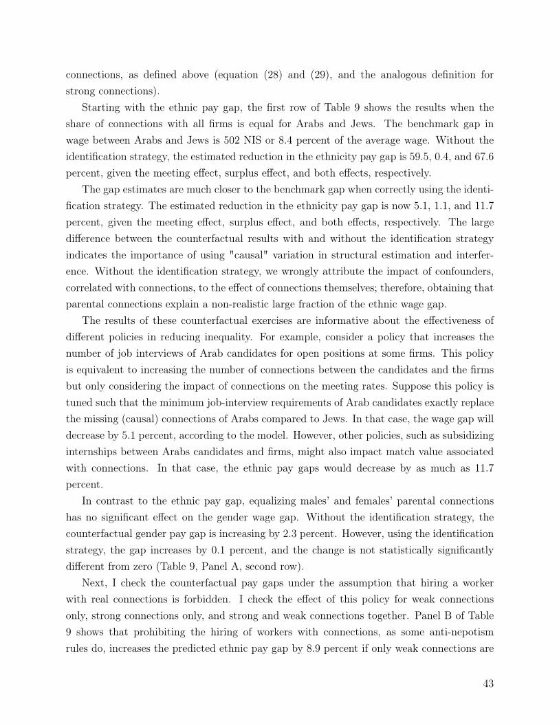
connections, as defined above (equation (28) and (29), and the analogous definition forstrong connections).

Starting with the ethnic pay gap, the first row of Table 9 shows the results when theshare of connections with all firms is equal for Arabs and Jews. The benchmark gap inwage between Arabs and Jews is 502 NIS or 8.4 percent of the average wage. Without theidentification strategy, the estimated reduction in the ethnicity pay gap is 59.5, 0.4, and 67.6percent, given the meeting effect, surplus effect, and both effects, respectively.

The gap estimates are much closer to the benchmark gap when correctly using the identi-fication strategy. The estimated reduction in the ethnicity pay gap is now 5.1, 1.1, and 11.7percent, given the meeting effect, surplus effect, and both effects, respectively. The largedifference between the counterfactual results with and without the identification strategyindicates the importance of using "causal" variation in structural estimation and interfer-ence. Without the identification strategy, we wrongly attribute the impact of confounders,correlated with connections, to the effect of connections themselves; therefore, obtaining thatparental connections explain a non-realistic large fraction of the ethnic wage gap.

The results of these counterfactual exercises are informative about the effectiveness ofdifferent policies in reducing inequality. For example, consider a policy that increases thenumber of job interviews of Arab candidates for open positions at some firms. This policyis equivalent to increasing the number of connections between the candidates and the firmsbut only considering the impact of connections on the meeting rates. Suppose this policy istuned such that the minimum job-interview requirements of Arab candidates exactly replacethe missing (causal) connections of Arabs compared to Jews. In that case, the wage gap willdecrease by 5.1 percent, according to the model. However, other policies, such as subsidizinginternships between Arabs candidates and firms, might also impact match value associatedwith connections. In that case, the ethnic pay gaps would decrease by as much as 11.7percent.

In contrast to the ethnic pay gap, equalizing males’ and females’ parental connectionshas no significant effect on the gender wage gap. Without the identification strategy, thecounterfactual gender pay gap is increasing by 2.3 percent. However, using the identificationstrategy, the gap increases by 0.1 percent, and the change is not statistically significantlydifferent from zero (Table 9, Panel A, second row).

Next, I check the counterfactual pay gaps under the assumption that hiring a workerwith real connections is forbidden. I check the effect of this policy for weak connectionsonly, strong connections only, and strong and weak connections together. Panel B of Table9 shows that prohibiting the hiring of workers with connections, as some anti-nepotismrules do, increases the predicted ethnic pay gap by 8.9 percent if only weak connections are

43

prohibited, 44.3 percent if only strong connections are prohibited, and 56.4 percent if bothweak and strong connections are prohibited. The gender pay gap declines by 4.0, 20.3, and25.3 percent, respectively, in these different scenarios.

The difference between the results of the two scenarios can be explained by consideringthe differences in the quality of connections and the "return" to connections of the differentgroups. For example, the model predicts that equalizing the connections between Arabs andJews reduces the ethnic pay gap, but prohibiting connections increases it. The explanationfor this comes from two opposing forces. On the one hand, Arabs have worse connections inthe labor market compared to Jews (Table 1 and Figure 1). On the other hand, the higherimpact of connections, obtained both in the reduced-form and structural estimation, indicatethat Arabs rely more heavily on connections compared to Jews (Figures 4 and 6). Therefore,equalizing Arabs and Jews’ connections provides them better connections, which reduces thepay gap. However, prohibiting the use of connections increases the gap as it hurts Arabsmore than Jews and increases the gap. The results of the gender gap are different. As thereis no big difference between the parental connections of males and females, equalizing theconnections does not impact the gender gap. However, because the return to connections ishigher for males than females, prohibiting connections hurts males more than females andreduces the gap.

8 Conclusion

In this paper, I study the role of parental social networks in shaping the distribution ofjob assignments and the wages of new workers. To do so, I leverage the timing of between-jobmoves of potential contacts relative to the labor-market entry year for exogenous variationof the social networks. In the first part of the paper, I use regression analysis to estimatethe effect of strong and weak parental connections on job assignments. Then, I build andestimate a matching model with search frictions where heterogeneous workers and firmschoose their best match given their choice set and the set of wages that clear the market. Iallow social connections to impact both the available choice sets and the match values.

In the first part, I find that workers are 3-4 times more likely to find employment infirms where a past coworker of the parent currently works than in otherwise similar firms. Ishow that the effect is more potent if the potential connections are formed in smaller firmsor, more recently. I also find a positive correlation between the wage of new workers andparental connections.

Estimates of the structural model show that parental connections increase the meetingprobability and the potential match value. Exploiting the same identification strategy, I

44

find that a weakly connected worker-firm pair is twice as likely to meet than a phantom-connected pair. Likewise, the match value is higher by 2.8 percent for weakly versus phantomconnected pairs. Using the model estimates, I find that workers are willing to pay, on average,3.7 percent of the average wage to get one additional meeting with a connected firm. I alsofind that differences in parental network quality explain a large proportion of Israel’s ethnicpay gap. Equalizing the quantity and quality of Arabs’ and Jews’ connections decreases theethnic pay gap by 12 percent. However, because Arabs rely more than Jews on connectedhiring, prohibiting the hiring of connected workers increases the gap by 56 percent.

My empirical results have nuanced consequences for policymakers. Policies to reducethe inequality implied by differential parental networks include, for example, subsidies forinternships in good firms for graduates with fewer connections or policies requiring interviewsof these candidates for open positions. The results of the model also shed light on theexpected outcomes of different policies. For instance, a long-term internship is likely toimpact not only the "search frictions" (e.g., the probability for a job interview at the firm) butalso the "match value" through better information on the workers and match quality. On theother hand, "Rooney Rule"-type policies are likely to impact only the "search frictions" andtherefore have a more moderate effect on inequality. Finally, the model suggests that policiesthat entirely prohibit the use of connections might have the opposite effect on inequality, asworkers from disadvantaged backgrounds rely more on social links in the labor market.

The framework employed here can be readily ported to other datasets and problems,and there is ample room for future research. First, like most of the matching literature,the model is static. Estimating a dynamic version of the model will enable studying howconnections matter over the life cycle and explicit modeling of the impact of referrals on thefirm’s uncertainty about worker quality. Additionally, observing the same workers over timeallows estimating workers’ and firms’ fixed effects, which cannot be separately identified ina static model. Second, having information on other labor market outcomes could allowthe estimation of additional unobserved parameters, such as the workers’ non-wage matchsurplus and differential workers’ bargaining power. Such data include direct information onfirms’ production or the meeting/interview process. Further unpacking the black box of thematching between workers and firms is essential in crafting policies to help reduce inequityin the labor market.

45

References

Abowd, John M., Francis Kramarz, and David N. Margolis, “High wage workersand high wage firms,” Econometrica, 1999, 67 (2), 251–333.

Agarwal, Nikhil, “An empirical model of the medical match,” American Economic Review,2015, 105 (7), 1939–78.

Ahyja, Ravindra K., James B. Orlin, and Thomas L. Magnanti, Network flows:theory, algorithms, and applications, Prentice-Hall, 1993.

Arellano-Bover, Jaime, “Career consequences of firm heterogeneity for young workers:First job and firm size,” Unpublished, 2020.

and Shmuel San, “The Role of Firms in the Assimilation of Immigrants,” Unpublished,2020.

Athey, Susan, Christopher Avery, and Peter Zemsky, “Mentoring and diversity,”American Economic Review, 2000, 90 (4), 765–786.

Azoulay, Pierre, Joshua S. Graff Zivin, and Jialan Wang, “Superstar extinction,”The Quarterly Journal of Economics, 2010, 125 (2), 549–589.

Bandiera, Oriana, Iwan Barankay, and Imran Rasul, “Social connections and in-centives in the workplace: Evidence from personnel data,” Econometrica, 2009, 77 (4),1047–1094.

Banfi, Stefano and Benjamin Villena-Roldan, “Do high-wage jobs attract more ap-plicants? Directed search evidence from the online labor market,” Journal of Labor Eco-nomics, 2019, 37 (3), 715–746.

Bayer, Patrick, Stephen L. Ross, and Giorgio Topa, “Place of work and place ofresidence: Informal hiring networks and labor market outcomes,” Journal of PoliticalEconomy, 2008, 116 (6), 1150–1196.

Beaman, Lori and Jeremy Magruder, “Who gets the job referral? Evidence from asocial networks experiment,” American Economic Review, 2012, 102 (7), 3574–93.

Berman, Eli, “Sect, subsidy, and sacrifice: an economist’s view of ultra-orthodox Jews,”The Quarterly Journal of Economics, 2000, 115 (3), 905–953.

46

Bernard, Florian, Nikos Vlassis, Peter Gemmar, Andreas Husch, Johan Thun-berg, Jorge Goncalves, and Frank Hertel, “Fast correspondences for statistical shapemodels of brain structures,” in “Medical Imaging 2016: Image Processing,” Vol. 9784 In-ternational Society for Optics and Photonics 2016, p. 97840R.

Berry, Steven, James Levinsohn, and Ariel Pakes, “Automobile prices in marketequilibrium,” Econometrica, 1995, pp. 841–890.

Bertsekas, Dimitri P., Network optimization: continuous and discrete models, AthenaScientific Belmont, MA, 1998.

Boca, Daniela Del and Christopher J. Flinn, “Household behavior and the marriagemarket,” Journal of Economic Theory, 2014, 150, 515–550.

Bolte, Lukas, Nicole Immorlica, and Matthew O. Jackson, “The Role of Referrals inInequality, Immobility, and Inefficiency in Labor Markets,” Unpublished, 2020.

Bonnet, Odran, Alfred Galichon, Keith O’Hara, and Matthew Shum, “YogurtsChoose Consumers? Estimation of Random Utility Models via Two-Sided Matching,”Unpublished, 2018.

Caldwell, Sydnee and Nikolaj Harmon, “Outside Options, Bargaining, and Wages:Evidence from Coworker Networks,” Unpublished, 2019.

and Oren Danieli, “Outside options in the labor market,” Unpublished, 2021.

Calvo-Armengol, Antoni and Matthew O. Jackson, “The effects of social networks onemployment and inequality,” American Economic Review, 2004, 94 (3), 426–454.

Card, David, Ana Rute Cardoso, Jörg Heining, and Patrick Kline, “Firms andlabor market inequality: Evidence and some theory,” Journal of Labor Economics, 2018,36 (S1), S13–S70.

CBS, “Social Survey 2016,” Technical Report, Central Bureau of Statistics, Jerusalem, Israel2018.

, “Statistical abstract of Israel,” Technical Report, Central Bureau of Statistics, Jerusalem,Israel 2019.

Chiappori, Pierre-André and Bernard Salanié, “The econometrics of matching mod-els,” Journal of Economic Literature, 2016, 54 (3), 832–61.

47

, , and Yoram Weiss, “Partner choice, investment in children, and the marital collegepremium,” American Economic Review, 2017, 107 (8), 2109–67.

Choo, Eugene and Aloysius Siow, “Who marries whom and why,” Journal of PoliticalEconomy, 2006, 114 (1), 175–201.

Cingano, Federico and Alfonso Rosolia, “People I know: job search and social networks,”Journal of Labor Economics, 2012, 30 (2), 291–332.

Cohen, Asher and Bernard Susser, “Jews and Others: Non-Jewish Jews in Israel,” IsraelAffairs, 2009, 15 (1), 52–65.

Corak, Miles and Patrizio Piraino, “The intergenerational transmission of employers,”Journal of Labor Economics, 2011, 29 (1), 37–68.

Demange, Gabrielle and David Gale, “The strategy structure of two-sided matchingmarkets,” Econometrica, 1985, pp. 873–888.

Dickinson, David L., David Masclet, and Emmanuel Peterle, “Discrimination asfavoritism: The private benefits and social costs of in-group favoritism in an experimentallabor market,” European Economic Review, 2018, 104, 220–236.

Dupuy, Arnaud and Alfred Galichon, “Personality traits and the marriage market,”Journal of Political Economy, 2014, 122 (6), 1271–1319.

and , “A Note on the Estimation of Job Amenities and Labor Productivity,” Unpub-lished, 2015.

Dustmann, Christian, Albrecht Glitz, Uta Schönberg, and Herbert Brücker,“Referral-based job search networks,” The Review of Economic Studies, 2016, 83 (2), 514–546.

Fontaine, Francois, “Why are similar workers paid differently? The role of social networks,”Journal of Economic Dynamics and Control, 2008, 32 (12), 3960–3977.

Fox, Jeremy T., Chenyu Yang, and David H. Hsu, “Unobserved heterogeneity inmatching games,” Journal of Political Economy, 2018, 126 (4), 1339–1373.

Fuchs, Hadas and Gil Epstein, “The Labor Market: An Overview,” State of the Nation:Policy, Economy and Society in Israel, 2019, pp. 139–162.

Galichon, Alfred and Bernard Salanié, “Cupid’s invisible hand: Social surplus andidentification in matching models,” Unpublished, 2020.

48

Galor, Oded and Daniel Tsiddon, “Technological progress, mobility, and economicgrowth,” American Economic Review, 1997, pp. 363–382.

Granovetter, Mark, Getting a job: A study of contacts and careers, University of Chicagopress, 1973.

Gretsky, Neil E., Joseph M. Ostroy, and William R. Zame, “Perfect competition inthe continuous assignment model,” Journal of Economic Theory, 1999, 88 (1), 60–118.

Hensvik, Lena and Oskar Nordström Skans, “Social networks, employee selection, andlabor market outcomes,” Journal of Labor Economics, 2016, 34 (4), 825–867.

Jaffe, Sonia and Simon Weber, “The effect of meeting rates on matching outcomes,”Economic Theory, 2019, 67 (2), 363–378.

Jager, Simon, “How substitutable are workers? evidence from worker deaths,” Unpublished,2016.

Kramarz, Francis and David Thesmar, “Social networks in the boardroom,” Journal ofthe European Economic Association, 2013, 11 (4), 780–807.

and Oskar Nordström Skans, “When strong ties are strong: Networks and youthlabour market entry,” Review of Economic Studies, 2014, 81 (3), 1164–1200.

Montgomery, James D., “Social networks and labor-market outcomes: Toward an eco-nomic analysis,” American Economic Review, 1991, 81 (5), 1408–1418.

Mortensen, Dale, Wage dispersion: why are similar workers paid differently?, MIT press,2003.

Mortensen, Dale T. and Christopher A. Pissarides, “Job creation and job destructionin the theory of unemployment,” The Review of Economic Studies, 1994, 61 (3), 397–415.

Noy, Chaim and Erik Cohen, Israeli backpackers: From tourism to rite of passage, SUNYPress, 2005.

Oreopoulos, Philip, Till Von Wachter, and Andrew Heisz, “The short-and long-term career effects of graduating in a recession,” American Economic Journal: AppliedEconomics, 2012, 4 (1), 1–29.

Plug, Erik, Bas van der Klaauw, and Lennart Ziegler, “Do Parental Networks Pay Off?Linking Children’s Labor-Market Outcomes to Their Parents’ Friends,” The ScandinavianJournal of Economics, 2018, 120 (1), 268–295.

49

Postel–Vinay, Fabien and Jean-Marc Robin, “Equilibrium wage dispersion with workerand employer heterogeneity,” Econometrica, 2002, 70 (6), 2295–2350.

Salanié, Bernard, “Identification in Separable Matching with Observed Transfers,” Unpub-lished, 2015.

Shapley, Lloyd S. and Martin Shubik, “The assignment game I: The core,” InternationalJournal of Game Theory, 1971, 1 (1), 111–130.

Solow, Benjamin L., John L. Solow, and Todd B. Walker, “Moving on up: TheRooney rule and minority hiring in the NFL,” Labour Economics, 2011, 18 (3), 332–337.

Staiger, Matthew, “The Intergenerational Transmission of Employers and the Earnings ofYoung Workers,” Unpublished, 2021.

Topa, Giorgio, “Labor markets and referrals,” in “Handbook of social economics,” Vol. 1,Elsevier, 2011, pp. 1193–1221.

50

Tables and Figures

Table 1: Summary statistics—new workers

All Ethnicity Gender

Jews Arabs Males Females

N. 220,806 157,023 63,783 126,233 94,573Arabs 0.29 0.00 1.00 0.37 0.19Females 0.43 0.49 0.28 0.00 1.00College 0.23 0.25 0.16 0.15 0.33

First jobAge 24.00 24.22 23.48 23.82 24.25Salary 5,839 6,053 5,312 6,223 5,325Tenure 2.01 1.97 2.10 2.04 1.98Firm rank 0.60 0.64 0.52 0.60 0.61Connections

Weak 0.03 0.02 0.04 0.03 0.02Strong 0.11 0.09 0.17 0.13 0.08

Age 30Salary 8,939 9,373 7,317 9,806 7,832Firm rank 0.68 0.70 0.58 0.67 0.68

ConnectionsAv. firm rank

Weak 0.64 0.66 0.58 0.63 0.65Strong 0.61 0.64 0.54 0.60 0.62

N. firmsWeak 43.66 50.40 26.78 41.71 46.26Strong 24.41 27.25 17.39 23.70 25.34

Notes: This table reports summary statistics for the sample of new workers. The first column reportsthe average value of the variables for the entire sample, and the other columns report for sub-samplesseparated according to ethnicity and gender. Firm rank is the rank of the firm-specific pay premiumestimated using an AKM model (Abowd et al. 1999). "Connections" indicates whether the workerhas weak or strong connections at the first job. Av. firm rank of connections is the average firmrank of firms with which the worker has weak and strong connections. N. firms is the number ofsuch firms.

51

Table 2: Effects of parental connections on firm assignment

All Jews Arabs Males Females

(1) (2) (3) (4) (5)

Phantom connections 0.010 0.006 0.030 0.011 0.008[0.009,0.011] [0.005,0.007] [0.025,0.032] [0.010,0.013] [0.006,0.010]

Weak connections 0.050 0.031 0.143 0.067 0.031[0.047,0.054] [0.028,0.034] [0.131,0.156] [0.061,0.071] [0.027,0.036]

Strong connections 0.487 0.366 0.917 0.617 0.338[0.472,0.501] [0.351,0.384] [0.878,0.956] [0.593,0.647] [0.320,0.354]

R0 (no connections) 0.005 0.005 0.006 0.005 0.006[0.005,0.005] [0.005,0.005] [0.006,0.006] [0.005,0.005] [0.005,0.006]

Ratio weak-phantom 3.666 3.259 4.177 4.409 2.731[3.316,4.081] [2.841,3.681] [3.651,4.803] [3.912,4.959] [2.262,3.303]

Ratio strong-phantom 32.52 33.99 25.91 38.37 25.37[30.02,35.53] [30.65,37.8] [23.52,30.03] [34.83,43.67] [22.41,29.39]

Observations 21,166,443 16,837,526 4,328,917 15,319,313 5,847,130N firms 149,729 144,186 117,746 145,939 134,555N groups 2,959 1,658 1,301 1,548 1,411N workers 220,684 157,009 63,675 170,872 49,812N connections 40,827,833 33,261,814 7,566,019 31,664,340 9,163,493

Notes: This table reports the probability of working in a firm with different types of connections,relative to working in a non-connected firm. The coefficients are the mean coefficients of phantom,weak, and strong connections across 100 estimations of equation (4) using a 20 percent randomsample of workers each time. The employment outcome is scaled by 100. I construct the bounds ofthe 95 percent confidence intervals using the 2.5 and 97.5 percentiles of the coefficients’ distribution.R0 is the average probability of working in a non-connected firm. "Ratio weak-phantom" is theestimated odds ratio between working at a weakly-connected firm and working in a phantom-connected firm. "Ratio strong-phantom" is defined similarly. The first column reports the resultsfor the entire sample, while the other columns report the results for a different sub-group of thenew workers each time.

52

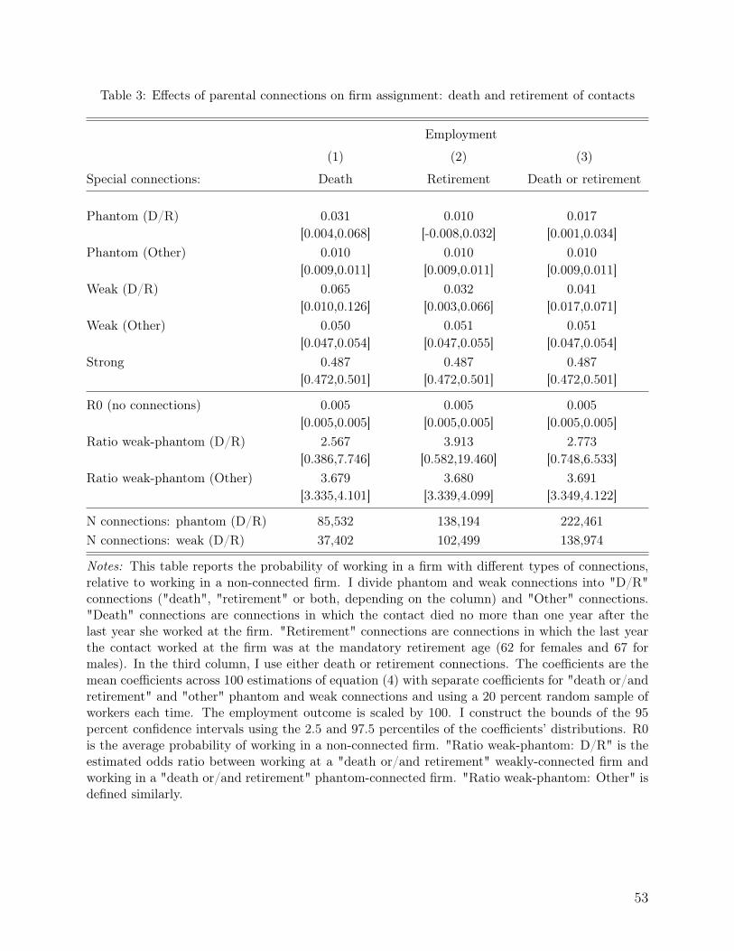
Table 3: Effects of parental connections on firm assignment: death and retirement of contacts

Employment

(1) (2) (3)

Special connections: Death Retirement Death or retirement

Phantom (D/R) 0.031 0.010 0.017[0.004,0.068] [-0.008,0.032] [0.001,0.034]

Phantom (Other) 0.010 0.010 0.010[0.009,0.011] [0.009,0.011] [0.009,0.011]

Weak (D/R) 0.065 0.032 0.041[0.010,0.126] [0.003,0.066] [0.017,0.071]

Weak (Other) 0.050 0.051 0.051[0.047,0.054] [0.047,0.055] [0.047,0.054]

Strong 0.487 0.487 0.487[0.472,0.501] [0.472,0.501] [0.472,0.501]

R0 (no connections) 0.005 0.005 0.005[0.005,0.005] [0.005,0.005] [0.005,0.005]

Ratio weak-phantom (D/R) 2.567 3.913 2.773[0.386,7.746] [0.582,19.460] [0.748,6.533]

Ratio weak-phantom (Other) 3.679 3.680 3.691[3.335,4.101] [3.339,4.099] [3.349,4.122]

N connections: phantom (D/R) 85,532 138,194 222,461N connections: weak (D/R) 37,402 102,499 138,974

Notes: This table reports the probability of working in a firm with different types of connections,relative to working in a non-connected firm. I divide phantom and weak connections into "D/R"connections ("death", "retirement" or both, depending on the column) and "Other" connections."Death" connections are connections in which the contact died no more than one year after thelast year she worked at the firm. "Retirement" connections are connections in which the last yearthe contact worked at the firm was at the mandatory retirement age (62 for females and 67 formales). In the third column, I use either death or retirement connections. The coefficients are themean coefficients across 100 estimations of equation (4) with separate coefficients for "death or/andretirement" and "other" phantom and weak connections and using a 20 percent random sample ofworkers each time. The employment outcome is scaled by 100. I construct the bounds of the 95percent confidence intervals using the 2.5 and 97.5 percentiles of the coefficients’ distributions. R0is the average probability of working in a non-connected firm. "Ratio weak-phantom: D/R" is theestimated odds ratio between working at a "death or/and retirement" weakly-connected firm andworking in a "death or/and retirement" phantom-connected firm. "Ratio weak-phantom: Other" isdefined similarly.

53

Table 4: Effect of weak parental connections on firm assignment, placebo test

All Jews Arabs Males Females

(1) (2) (3) (4) (5)

Phantom connections 0.000 0.000 0.000 0.000 0.000[-0.001,0.001] [-0.001,0.001] [-0.002,0.003] [-0.001,0.001] [-0.001,0.001]

Weak connections 0.000 0.000 0.000 0.000 0.000[-0.002,0.002] [-0.002,0.002] [-0.006,0.006] [-0.002,0.003] [-0.003,0.003]

Strong connections 0.000 0.000 0.001 0.000 0.000[-0.006,0.007] [-0.005,0.005] [-0.021,0.021] [-0.006,0.008] [-0.008,0.010]

R0 (no connections) 0.007 0.006 0.011 0.008 0.007[0.007,0.008] [0.006,0.007] [0.011,0.012] [0.007,0.008] [0.007,0.007]

Ratio weak-phantom 1.010 1.000 1.053 1.011 1.017[0.755,1.384] [0.727,1.330] [0.397,1.645] [0.660,1.334] [0.631,1.524]

Ratio strong-phantom 1.047 1.029 1.107 1.065 1.036[0.206,2.019] [0.189,1.805] [-0.938,3.233] [0.154,1.981] [-0.162,2.471]

Observations 21,166,443 16,837,526 4,328,917 15,319,313 5,847,130N firms 149,729 144,186 117,746 145,939 134,555N groups 2,959 1,658 1,301 1,548 1,411N workers 220,684 157,009 63,675 170,872 49,812N connections 40,827,833 33,261,814 7,566,019 31,664,340 9,163,493

Notes: This table shows placebo test results, assigning the worker’s connections to a random workerin her group. The table reports the probability of working in a firm with different types of con-nections, relative to working in a non-connected firm, based on the new (randomized) data. Thecoefficients are the mean coefficients of phantom, weak, and strong connections across 100 esti-mations of equation (4) using a 20 percent random sample of workers each time. I construct thebounds of the 95 percent confidence intervals using the 2.5 and 97.5 percentiles of the coefficients’distributions. The employment outcome is scaled by 100. R0 is the average probability of workingin a non-connected firm. "Ratio weak-phantom" is the estimated odds ratio between working at aweakly-connected firm and working in a phantom-connected firm. "Ratio strong-phantom" is de-fined similarly. The first column reports the results for the entire sample, while the other columnsreport the results for a different sub-group of the new workers each time.

54

Table 5: Correlation between parental connections at first job and salary and tenure

Log salary Job tenure

(1) (2) (3) (4)

Phantom connections -0.007 0.012 0.123 0.098(0.005) (0.004) (0.022) (0.022)

Weak connections 0.018 0.026 0.182 0.187(0.005) (0.004) (0.024) (0.025)

Strong connections 0.074 0.083 0.601 0.441(0.004) (0.003) (0.024) (0.020)

Group FE Yes Yes Yes YesFirm FE No Yes No YesObservations 220,806 220,806 220,806 220,806N firms 54,321 54,321 54,321 54,321R2 (full model) 0.169 0.624 0.127 0.414R2 (projected model) 0.004 0.006 0.014 0.007

Notes: This table reports the correlation between parental connections of different types and thesalary and tenure at the first job. The outcome variable in the first two columns is (log) monthlysalary in the first year of the first job. The outcome variable in the last two columns is the numberof sequential years the worker worked at the first job (truncated at 2015). All specifications includegroup fixed effects. The second and forth specifications also include firm fixed effects. Groups areconstructed using all combinations of the workers’ observable characteristics (ethnicity, education,gender, year of first job, age, and district of residence). Robust standard errors clustered by groupand firm are reported in parentheses.

55

Table 6: Model’s fit, Model’s precision, and Monte Carlo simulation

A. Model’s fit

Matches Av. wage Overall Within-group(µtxyc) (wtxyc) wage variance wage variance

(1) (2) (3) (4)

Abs. deviation 0.013 0.008 0.0008 0.0007(0.0006) (0.0006) (0.0006) (0.0005)

Correlation 1.000 0.998(0.00002) (0.0002)

B. Model’s precision and Monte Carlo simulation

Surplus Meetings Unobserved Surplus(βtxyc) (ptxyc) heterogeneity (log(σ)) scale (b)

(1) (2) (3) (4)

EstimatesCorrelation 0.980 0.988

(0.001) (0.0006)Value -1.069 9.174

(0.007) (0.011)Monte CarloCorrelation 0.972 0.985

(0.003) (0.0006)Value -1.076 9.186

(0.006) (0.009)

Notes: This table reports measures of the model’s fit to the data (Panel A), the model’s precision, andthe results of Monte Carlo simulation (Panel B). The first row reports the average difference between thepredicted and true moments on a logarithmic scale (averaged over all txyc cells with weights equal tothe observed matches in each cell µtxyc in the first two columns). The second row of Panel A shows thecorrelation between the true and predicted moments (with the same weights). Each statistic in Panel A iscalculated separately for each of the 100 estimations of the model, and the table reports the averages acrossthe 100 estimations (and their standard errors in parentheses). The first row of Panel B reports the averagecorrelation in the surplus and meeting parameters across any possible pair within the 100 estimations (andtheir standard errors in parentheses). The second row reports the average values (and standard errors) ofthe unobserved heterogeneity σ, and utility-scale b parameters across the 100 simulations. The last tworows report the results of Monte Carlo simulation, where I use the average parameter values as the "trueparameters" to generate data and estimate the model 100 times again with different idiosyncratic shocks. Thethird row reports the average correlation in the surplus and meeting parameters between the new estimatesand the "true parameters". The final row shows the average value of the other two parameters. Standarderrors across the 100 Monte Carlo estimations are reported in parentheses.

56

Table 7: Projection of the model estimates on workers’, firms’, and connections’ characteristics

Meeting probability (Log(ptxyc)) Firm’s surplus (βtxyc)

(1) (2)

Constant -6.900 8.809(0.015) (0.011)

Phantom connections 1.964 0.012(0.039) (0.007)

Weak connections 2.728 0.041(0.038) (0.008)

Strong connections 3.742 0.158(0.019) (0.004)

Arab 0.051 -0.011(0.010) (0.002)

Female -0.009 -0.070(0.010) (0.002)

College -0.066 0.077(0.011) (0.002)

Job type: 2 -0.067 0.120(0.012) (0.005)

Job type: 3 -0.028 0.268(0.012) (0.005)

Job type: 4 -0.002 0.459(0.013) (0.006)

Job type: 5 -0.093 0.967(0.021) (0.007)

Weak - phantom 0.764 0.028(0.054) (0.010)

Strong - phantom 1.779 0.146(0.042) (0.008)

R2 0.831 0.907(0.005) (0.003)

Notes: This table reports the results of regressing the meeting and surplus estimates on worker,firm, and connection characteristics. I estimate the regression using weighted least squares, withweights equal to the actual number of matches of the txyc cell. "Weak (Strong) - phantom" is thedifference between the coefficients of weak (strong) and phantom connections. Each regression iscalculated separately for each of the 100 estimations of the model, and the table reports the averagesacross the 100 estimations (and their standard errors in parentheses).

57

Table 8: Value of meetings and connections

Total expected gains Salary change with a job change Salary change without a job change

Probability Gains Expected gains Probability Gains Expected gains

(1) (2) (3) (4) (5) (6) (7)

New meeting, without surplus effect 2.2 0.040 41.4 1.7 0.064 7.9 0.5(0.417) (0.007) (6.543) (0.394) (0.008) (1.809) (0.135)

Existing meeting, with surplus effect 1.5 0.040 20.3 0.8 0.101 6.4 0.7(0.467) (0.007) (8.151) (0.373) (0.010) (2.974) (0.311)

New meeting, with surplus effect 3.7 0.055 57.0 3.1 0.066 9.0 0.6(0.819) (0.009) (9.323) (0.778) (0.008) (2.248) (0.153)

Notes: This table shows the impact of a new meeting or connection on the average worker’s expected value (in terms of percentages ofnew workers’ average wage). Each row reports the average change in the salary of workers in one of three different scenarios: 1) adding ameeting to a random worker and firm in each market, assuming no connections between them, 2) choosing a random non-connected pairin each market and changing the systematic match surplus to reflect the surplus of a causal weak connection, and 3) adding a randommeeting with causal weak connections. The surplus of a causal weak connection is the excess surplus of weak connections compared tophantom connections. The first column reports the total expected gains. In the rest of the columns, I decompose that effect into twoevents. In columns (2)-(4), the new meeting or connection impacts the identity of the firm the worker ends up working at (compared tothe job before the change). In the last three columns, the worker stays in the same position with and without the shock, but her salarychanges due to a change in the available choice set. For each event, I report the probability of this event to happen, the average gains, andthe expected gains of this event (probability multiplied by gains). Each statistic is calculated separately for each of the 100 estimationsof the model, based on 1,000 new meetings/connections for each estimation, and the table reports the averages across the 100 estimations(and their standard errors in parentheses).

58

Table 9: Counterfactual impacts of connections on between-group pay gaps

A. Equalizing number of connections per worker

Gap Without identification strategy With identification strategy

(% Average) Meetings effect Surplus effect Both effects Meetings effect Surplus effect Both effects

(1) (2) (3) (4) (5) (6) (7)

Ethnicity gap -8.4 -59.5 -0.4 -67.6 -5.1 -1.1 -11.7(0.351) (4.866) (0.168) (3.031) (0.679) (0.297) (1.638)

Gender gap -18.0 1.2 0.0 2.3 0.1 0.0 0.1(0.290) (0.180) (0.034) (0.197) (0.066) (0.045) (0.093)

B. Prohibiting hiring of connected workers

Baseline Weak Strong Weak + strong

(% Average)

(1) (2) (3) (4)

Ethnicity gap -8.4 8.9 44.3 56.4(0.351) (0.982) (2.820) (3.347)

Gender gap -18.0 -4.0 -20.3 -25.3(0.290) (0.320) (0.780) (0.798)

Notes: This table shows the contribution of parental connections to the ethnic and gender pay gaps in two scenarios. Panel A reports estimates fromequalizing the connections between the ethnic and gender group. Specifically, in the first row, I present the ethnic pay gap predicted by the modelassuming each group of Arabs and Jews (with similar gender and education characteristics) have the same number of weak and strong connectionsper worker with every type of firm. The second row reports the analogous results for the gender gap. Column (1) reports the benchmark pay gapas a share of the average wage. In columns (2)-(5), I estimate the counterfactual pay gaps under the assumption that new connections (either weakor strong) have the same impact on the meeting rate and the match surplus as a real connection of the same type in the same txyc cell. In columns(6)-(8), I assume that the impact of new connections on the meeting rate and the match surplus is the excess impact of strong or weak connections onthese parameters compared to phantom connections ("causal connections"). In columns (2) and (5), I shut down the surplus effect of new connections(assuming they are similar to the surplus of that txyc group without connections) to examine the impact of the meeting rate alone. Similarly, incolumns (2) and (5), I shut down the meetings effect. In columns (4) and (7), I estimate the ethnic wage gap with both effects. Panel B reportsthe estimated gaps from the scenario that hiring of connected workers is prohibited. Columns (2), (3), and (4) assume hiring of workers with weak,strong, or either is banned, respectively. Each statistic is calculated separately for each of the 100 estimations of the model, and the table reports theaverages across the 100 estimations (and their standard errors in parentheses).

59

Figure 1: Average connected firms per worker by worker characteristics, firm type, andconnection type

0

5

10

15

20

1 2 3 4 5Firm type

Ave

rgae

con

nect

ions

per

wor

ker

JewsArabs

A. Weak connections by ethnicity

0

5

10

15

20

1 2 3 4 5Firm type

Ave

rgae

con

nect

ions

per

wor

ker

JewsArabs

B. Strong connections by ethnicity

0

5

10

15

20

1 2 3 4 5Firm type

Ave

rgae

con

nect

ions

per

wor

ker

MalesFemales

C. Weak connections by gender

0

5

10

15

20

1 2 3 4 5Firm type

Ave

rgae

con

nect

ions

per

wor

ker

MalesFemales

D. Strong connections by gender

Notes: This figure shows the average number of weakly and strongly connected firms perworker by workers’ ethnicity and gender, and by quintiles of the AKM firm premium, aver-aged over the years 2006-2015.

60

Figure 2: Event-study plot of coefficients: Effect of weak parental connections on firm as-signment

0.00

0.02

0.04

0.06

0.08

−5 −4 −3 −2 −1 0 1 2 3 4 5Last year parent's coworker worked at the firm relative to child's labor−market entry year

Exc

ess

prob

abili

ty o

f wor

king

at t

he fi

rm

Notes: This figure shows the probability of working in a firm as a function of the differencebetween the last year the parent’s coworker worked at the firm and the worker’s labor-market entry year, relative to working in a non-connected firm. The points are the meancoefficients of phantom and weak connections across 100 estimations of equation (5) usinga 20 percent random sample of workers each time. The employment outcome is scaled by100. I construct the bounds of the 95 percent confidence intervals using the 2.5 and 97.5percentiles of the coefficients’ distribution. The vertical line between -1 and 0 indicates thechange from worker-firm pairs with phantom connections to pairs with weak connections.

61

Figure 3: Event-study plot of coefficients: Effect of weak parental connections on firm as-signment, placebo test

0.00

0.02

0.04

0.06

0.08

−5 −4 −3 −2 −1 0 1 2 3 4 5Last year parent's coworker worked at the firm relative to child's labor−market entry year

Exc

ess

prob

abili

ty o

f wor

king

at t

he fi

rm

Notes: This figure reports the results of a placebo test, assigning the worker’s connectionsto a random worker in her group. The figure shows the probability of working in a firm asa function of the difference between the last year the parent’s coworker worked at the firmand the worker’s labor-market entry year, relative to the probability of working in a non-connected firm, based on the new (randomized) data. The points are the mean coefficientsof phantom and weak connections across 100 estimations of equation (5) using a 20 percentrandom sample of workers each time. The employment outcome is scaled by 100. I constructthe bounds of the 95 percent confidence intervals using the 2.5 and 97.5 percentiles of thecoefficients’ distribution. The vertical line between -1 and 0 indicates the change fromworker-firm pairs with phantom connections to pairs with weak connections.

62

Figure 4: Effects of weak parental connections on firm assignment: Heterogeneity by char-acteristics of the workers and the connections

0.0

0.1

0.2

0.3

1 2 3 4 5 6 7 8 9 10Bin

A. Parent's firm size

0.0

0.1

0.2

0.3

1 2 3 4 5 6 7 8 9 10Bin

B. Parent's salary rank: overall

0.0

0.1

0.2

0.3

1 2 3 4 5 6 7 8 9 10Bin

C. Parent's salary rank: firm

0.0

0.1

0.2

0.3

1 2 3 4 5 6 7 8 9 10Bin

D. Coworker's past salary rank: overall

0.0

0.1

0.2

0.3

1 2 3 4 5 6 7 8 9 10Bin

E. Coworker's past salary rank: firm

0.0

0.1

0.2

0.3

1 2 3 4 5 6 7 8 9 10Bin

F. Coworker's current firm size

0.0

0.1

0.2

0.3

1 2 3 4 5 6 7 8 9 10Bin

G. Parent−coworker rank difference: firm

0.00.10.20.30.4

1 2 3 4 5 6 7 8 9 10Years

H. Length of co−working

0.0

0.1

0.2

0.3

1 2 3 4 5 6 7 8 9 101112131415Years

I. Time since co−working

0.0

0.1

0.2

0.3

Female Male

J. Child's gender

0.0

0.1

0.2

0.3

Female Male

K. Parent's gender

0.0

0.1

0.2

0.3

Female Male

L. Coworker's gender

0.0

0.1

0.2

0.3

Arab Jew

M. Child's ethnicity

0.0

0.1

0.2

0.3

Arab Jew

N. Coworker's ethnicity

0.0

0.1

0.2

0.3

College No college

O. Child's education

0.0

0.1

0.2

0.3

Different Same

P. Gender child−parent

0.0

0.1

0.2

0.3

Different Same

Q. Gender child−coworker

0.0

0.1

0.2

0.3

Different Same

R. Ethnicity child−coworker

Notes: Each figure shows the probability of working in a firm with weak connections for different charac-teristics of the workers and the connections, relative to the probability of working in a phantom-connectedfirm. The points are the mean coefficients of weak connections across 100 estimations of equation (1) withseparate coefficients for different groups of weak and phantom connections, using a 20 percent random sampleof workers each time. The employment outcome is scaled by 100. I construct the bounds of the 95 percentconfidence intervals using the 2.5 and 97.5 percentiles of that distribution of coefficients.

63

Figure 5: Scatter plot: Changes in moments as a result of changes in parameters of the samegroup of workers and firms

−4

−2

0

2

4

−1.0 −0.5 0.0 0.5 1.0Change in match surplus

Cha

nge

in a

ssig

nmen

ts

A. Matches−surplus

−4

−2

0

2

4

−1.0 −0.5 0.0 0.5 1.0Change in meetings probability

Cha

nge

in a

ssig

nmen

ts

B. Matches−meetings

−4

−2

0

2

4

−1.0 −0.5 0.0 0.5 1.0Change in match surplus

Cha

nge

in w

ages

C. Wages−surplus

−4

−2

0

2

4

−1.0 −0.5 0.0 0.5 1.0Change in meetings probability

Cha

nge

in w

ages

D. Wages−meetings

Notes: This figure shows the relationships between the parameters of the model and thepredicted moments. I run 10,000 simulations of the model. Each time, I change the value ofonly one parameter, either the match surplus βtxyc or the meeting probability ptxyc, of onexyc group in each market t by a random number between -1 and 1. Each graph’s y-axis isthe difference between the (log) number of matches and (log) average wage predicted by themodel with the new parameters and the moments predicted with the old parameters. Thex-axis is the size of the change to the parameters, β and log(p). The plots show only theresults of the moment changes in the txyc cells for which the parameter was changed.

64

Figure 6: Model estimates: Average meeting probability by workers’ group and connectiontype

−7

−6

−5

−4

−3

None

Phant

omW

eak

Strong

Causa

l wea

k

Causa

l stro

ng

Log

mee

ting

prob

abili

ty JewsArabs

A. Ethnicity

−7

−6

−5

−4

None

Phant

omW

eak

Strong

Causa

l wea

k

Causa

l stro

ng

Log

mee

ting

prob

abili

ty MalesFemales

B. Gender

Notes: This figure shows the results of regressing the log of the meeting probabilities obtainedfrom the model on worker, firm, and connection characteristics, and the interactions betweenworker and connection features. I estimate the regression using weighted least squares, withweights equal to the actual number of matches of the txyc cell. Each point on the graph isthe meeting probability by ethnicity and connections type predicted by this regression. Eachregression is calculated separately for each of the 100 estimations of the model, and the tablereports the averages across the 100 estimations (and their 95% confidence intervals).

65

Appendices

A Appendix Tables and Figures

Table A1: Summary statistics—firms

1-4 5-500 501+

Firms 123,677 51,999 392Workers 225,830 1,155,398 833,097Av. firm size 1.83 22.23 2131.56Share of firms 0.702 0.296 0.002Share of workers 0.102 0.522 0.376

Notes: This table reports summary statistics for firms according to the number of workers in thefirm. The first row is the overall number of unique firms in 2006-2015 matched employee-employerfiles. The second row is the total number of workers in each group of firms by year, averaged acrossthe years. The third row is the average number of workers in a firm by year, averaged across theyears. The fourth and fifth rows are the share of firms and the share of workers in each group offirms by year, averaged across the years.

66

Table A2: Balancing test: Correlation between parental connections and measures of proximitybetween workers and firms

Log distance Parent’s industry

(1) (2)

Phantom connections -0.369 0.077[-0.376,-0.362] [0.076,0.077]

Weak connections -0.368 0.076[-0.375,-0.361] [0.075,0.076]

Strong connections -0.926 0.281[-0.944,-0.909] [0.279,0.284]

R0 (no connections) 10.102 0.033[10.090,10.117] [0.032,0.033]

Ratio weak-phantom 1.000 0.989[1.000,1.001] [0.984,0.995]

Ratio strong-phantom 0.943 2.871[0.942,0.944] [2.850,2.887]

Observations (firms x groups) 21,166,443 21,166,443N firms 149,729 149,729N groups 2,959 2,959N workers 220,684 220,684

Notes: This table reports the (log) geographical distance from the firm and the probability thata firm belongs to the same 3-digit industry of the worker’s parent for firms with different types ofconnections, relative to non-connected firms. The coefficients are the mean coefficients of phantom,weak, and strong connections across 100 estimations of equation (4) with the outcome variablesmentioned using a 20 percent random sample of workers each time. I construct the bounds of the95 percent confidence intervals using the 2.5 and 97.5 percentiles of the coefficients’ distribution.R0 is the average outcome variable’s value for a non-connected firm. "Ratio weak-phantom" isthe estimated odds ratio between the outcome variable’s value for a weakly-connected firm andphantom-connected firm. "Ratio strong-phantom" is defined similarly.

67

Table A3: Effects of parental connections on firm assignment: Robustness to the definition ofconnection types

Employment

(1) (2) (3)

Phantom (single contact) 0.010 0.012[0.009,0.011] [0.011,0.013]

Phantom (single + multiple contacts) 0.015[0.014,0.016]

Weak (signle contact) 0.050 0.053[0.047,0.054] [0.049,0.056]

Weak (single + multiple contacts) 0.095[0.091,0.100]

Strong (direct + multiple contacts) 0.487[0.472,0.501]

Direct 3.091 3.092[2.977,3.206] [2.978,3.207]

Multiple contacts 0.171[0.161,0.181]

R0 (no connections) 0.005 0.005 0.005[0.005,0.005] [0.005,0.005] [0.005,0.005]

Observations (firms x groups) 21,166,443 21,166,443 21,166,443N firms 149,729 149,729 149,729N groups 2,959 2,959 2,959N workers 220,684 220,684 220,684N connections 40,827,833 40,827,833 40,827,833

Notes: This table reports the probability of working in a firm with different types of connections,relative to working in a non-connected firm. The coefficients are the mean coefficients of the differenttypes of connections across 100 estimations of the equivalent of equation (4) using a 20 percentrandom sample of workers each time. I construct the bounds of the 95 percent confidence intervalsusing the 2.5 and 97.5 percentiles of the coefficients’ distributions. The employment outcome isscaled by 100. R0 is the average probability of working in a non-connected firm. The first columnrepeats the baseline specification using three types of connections: phantom connection with a singlecontact, indirect connection with a single contact ("weak"), and either a direct connection or othertypes of connection with more than one contact ("strong"). Column 2 estimates a separate coefficientfor direct connections and for phantom/indirect connections with multiple contacts. Column 3combines phantom and indirect connections with one or more contacts.

68

Table A4: Event-study plot of coefficients: Effect of parental connections on firm assignment

Employment

Phantom connections Weak connections

-5 0.005 0 0.057[0.002,0.009] [0.052,0.063]

-4 0.005 1 0.052[0.003,0.008] [0.043,0.060]

-3 0.007 2 0.042[0.004,0.009] [0.033,0.053]

-2 0.009 3 0.040[0.006,0.013] [0.030,0.053]

-1 0.012 4 0.050[0.008,0.015] [0.035,0.067]

1 0.026 5 0.040[0.020,0.032] [0.032,0.048]

2 0.017 Strong connections[0.013,0.022]

3 0.013 0.487[0.009,0.017] [0.472,0.501]

4 0.009[0.006,0.014]

5 0.008[0.005,0.011]

Notes: This table reports the probability of working in a firm for a different types of connectionsrelative to working in a non-connected firm. Phantom and weak connections are divided accordingto the difference between the last year the parent’s coworker worked at the firm and the child’slabor-market entry year. The points are the mean coefficients across 100 estimations of equation(5) using a 20 percent random sample of workers each time. The employment outcome is scaled by100. I construct the bounds of the 95 percent confidence intervals using the 2.5 and 97.5 percentilesof the coefficients’ distribution.

69

Table A5: Moments-parameters elasticities

Matches-surplus Matches-meetings Wages-surplus Wages-meetings

dln(µ)/dβ dln(µ)/dln(p) dln(w)/dβ dln(w)/dln(p)

(1) (2) (3) (4)

Same workers and firms 3.511 0.777 3.427 0.015(0.078) (0.017) (0.325) (0.009)

Same workers, different firms -0.264 -0.033 0.001 0.014(0.026) (0.003) (0.011) (0.001)

Different workers -0.008 0.000 -0.032 -0.002(0.002) (0.000) (0.005) (0.000)

Notes: This table shows the elasticities between the parameters of the model and the predictedmoments. I run 10,000 simulations of the model. Each time, I change the value of only oneparameter, either the match surplus βtxyc or the meeting probability ptxyc, of one xyc group in eachmarket t by a random number between -1 and 1. Each value in the table is the slope coefficientobtained from regressing the changes in the moment on the parameter changes for different groupsof workers and firms. Assume a change in the txyc cell parameters. The first row reports theelasticities of changes in the same txyc cells. The second row reports the elasticities for cells of thetype txy′c′ where either y′ 6= y or c′ 6= c (or both). The last row reports the elasticities for cells ofthe type tx′y′c′ where x′ 6= x. Each statistic is calculated separately for each of the 100 estimationsof the model, based on 1,000 new meeting/surplus parameters for each estimation, and the tablereports the averages across the 100 estimations (and their standard errors in parentheses).

70

Figure A1: Raw data: probability of working in a firm for phantom and weak connections

0.00

0.05

0.10

0.15

−5 −4 −3 −2 −1 0 1 2 3 4 5Last year parent's coworker worked at the firm relative to child's labor−market entry year

Pro

babi

lity

of w

orki

ng a

t the

firm

Notes: This figure shows the raw probability of working in a firm as a function of thedifference between the last year the parent’s coworker worked at the firm and the worker’slabor-market entry year. The employment outcome is scaled by 100. The vertical linebetween -1 and 0 indicates the change from worker-firm pairs with phantom connections topairs with weak connections.

71

Figure A2: Age at last year of work by gender

0.025

0.050

0.075

50 60 70 80Age

Fre

quen

cy

A. Males

0.000

0.025

0.050

0.075

50 60 70 80Age

Fre

quen

cy

B. Females

Notes: This figure shows the frequency of the ages of workers when they last appear in theemployer-employee data between 2006-2014, separated by gender. Workers that worked in2015—the final year in the dataset—are not included in this figure. I keep workers that werebetween 50-80 in their last year of work.

72

Figure A3: Scatter plot: Lower and upper wage bounds

−10000

0

10000

20000

−15000 −10000 −5000 0 5000 10000Wage lower bound

Wag

e up

per

boun

d

Notes: This figure shows the relationships between lower and upper wage bounds thatsupport the equilibrium matching. The black line shows the mean value of the wage upperbounds for 100 bins of the lower bounds.

73

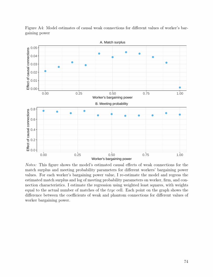
Figure A4: Model estimates of causal weak connections for different values of worker’s bar-gaining power

0.00

0.01

0.02

0.03

0.04

0.05

0.00 0.25 0.50 0.75 1.00Worker's bargaining power

Effe

ct o

f cau

sal c

onne

ctio

ns

A. Match surplus

0.0

0.2

0.4

0.6

0.8

0.00 0.25 0.50 0.75 1.00Worker's bargaining power

Effe

ct o

f cau

sal c

onne

ctio

ns

B. Meeting probability

Notes: This figure shows the model’s estimated causal effects of weak connections for thematch surplus and meeting probability parameters for different workers’ bargaining powervalues. For each worker’s bargaining power value, I re-estimate the model and regress theestimated match surplus and log of meeting probability parameters on worker, firm, and con-nection characteristics. I estimate the regression using weighted least squares, with weightsequal to the actual number of matches of the txyc cell. Each point on the graph shows thedifference between the coefficients of weak and phantom connections for different values ofworker bargaining power.

74

Figure A5: Value of a meeting by job type

0

2

4

6

8

1 2 3 4 5Job type

Wor

ker's

tota

l exp

ecte

d ga

ins

New meeting, without surplus effectExisting meeting, with surplus effectNew meeting, with surplus effect

Notes: This figure shows the impact of a new meeting or connection on the average worker’sexpected value separated according to the type of firm with which the meeting/connectionis generated. Each line reports the average change in the salary of workers in one of threedifferent scenarios: 1) adding a meeting to a random worker and firm in each market, as-suming no connections between them, 2) choosing a random non-connected pair in eachmarket and changing the systematic match surplus to reflect the surplus of a causal weakconnection, and 3) adding a random meeting with causal weak connections. The surplus ofa causal weak connection is the excess surplus of weak connections compared to phantomconnections. Each statistic is calculated separately for each of the 100 estimations of themodel, based on 1,000 new meetings/connections for each estimation, and the table reportsthe averages across the 100 estimations.

75

B Data Appendix

This appendix provides additional details on the data preparation and definitions of thevariables.

Employment and wages: The data contain observations at the worker × firm ×year level. For each observation, there are monthly employment indicators and total yearlysalaries. In each year, I: 1) drop observations with missing worker or firm identifiers, 2)replace empty monthly indicators with zeros, 3) drop observations that are duplicate inall variables, 4) for duplicate worker-firm observations, take the maximum of the monthlyindicators and the sum of the yearly earnings, 5) calculate the monthly salary by dividingthe yearly salary by the number of months worked at that firm, 6) keep only observationswith employment in February, 7) for each worker, keep the firm with the largest monthlysalary 8) keep workers aged 22-69, 9) drop observations with less than 25% of the yearlyaverage wage in the sample.

Parents and Children: The data include the identifiers of the mother and the fatherof each Israeli citizen, provided that they are also Israeli citizens.

Education: "No college" workers are defined as workers without any period of enroll-ment in higher education institutions. Workers with at least one year of admission to highereducation institutions (excluding religious schools) are defined as workers with "some college"or simply with "college" education.

Ethnicity: Workers are classified into two categories, Arabs and Jews. Arabs includeArab Muslims, Arab Christians, Druze, and Circassians. In the definition of Jews, I followthe practice of the Israeli Central Bureau of Statistics to include "Jews and Others" togetherand consider workers without ethnicity classification as Jews.49

Workers’ location: I measure the new worker’s residence location by the longitude andlatitude of the centroid of the city she lived in at age 21. I also use the worker’s district atage 21, one of seven districts (North, Haifa, Tel-Aviv, Center, Jerusalem, South, and Judeaand Samaria).

Natives: Individuals born in Israel and without information on the date of immigration.Ultra-orthodox: I use the internal algorithm of the National Insurance Institute, which

uses information on the residency neighborhoods, educational institutions, and family linksto identify Ultra-orthodox individuals.

Industry: I clean the industry variable such that each firm has a unique industry. Using49According to the Israeli Central Bureau of Statistics definitions, "Others" refer to Non-Arab Christians,

members of other religions, and not classified (CBS 2019). The majority of the people in this category areimmigrants from the former Soviet Union who immigrated to Israel in the past three decades. They are notJews according to the Jewish law but are included in the Law of Return because of their familial ties withJew (Cohen and Susser 2009).

76

the same employer-employee row file described above, with additional information on the4-digit industry code of the firm in each observation, In each year, I: 1) drop observationswith missing worker, firm, or industry identifiers, 2) for each firm, keep the industry withthe most occurrences. Now, if the number of firms in industry A in year t that changed theirindustry in year t + 1 to B is greater than the number of firms that stay in industry A, Iassume the classification of that industry had changed and update backward industry A toB. Finally, for each firm, I keep the latest industry. In practice, I use the implied 3-digitindustry code of each firm.

Firms’ location: Unfortunately, exact information on the location of the firms is miss-ing. As a proxy, I calculate the median longitude and latitude of the residence of the workers.I exclude new workers from the calculation of the firms’ locations.50

Firms’ pay premium: I estimate the following AKM model (Abowd et al. 1999)

wit = αi + ψJ(it) + Z ′itγ + εit (B1)

where αi is person fixed effect, ψJ(it) is firm fixed effect, Z ′it = are set of year fixed effectsand quartic polynomials age-restricted to be flat at age 40 (Card et al. 2018). I estimate themodel using workers ages 22-69. I exclude new workers, so their salary would not impactthe estimated firm premiums. To capture potential changes in a given firm’s premium overthe years, I estimate a separate regression each year. Precisely, firm premiums of firms atyear t are calculated using the full sample’s largest connected set in years [t− 4, t]. Finally,I rank the estimated firm premiums within a year ("firm rank").

50The data do not include establishment/plant identifiers or an indicator for multi-plant firms. Therefore,I assign the same location for all branches or plants of the same firm. This problem is alleviated by droppingfirms with more than 500 workers from the sample.

77

C The role of firms and social networks in earnings inequal-

ity

In this appendix, I decompose the ethnic and gender pay gaps into between- and within-firm variation. I also check the correlation of these gaps with measures of connection quality.

To get the raw ethnic and gender gaps, I estimate the equation

wi = γ1 · Arabi + γ2 · Femalei + φx(i) + εi (C1)

using all workers ages 22-69 in Israel in 2015. wi is the log wage of worker i, Arabi andFemalei equal 1 if worker i is an Arab or female, respectively. φx(i) and ψj(i) are groupand firm fixed effects, respectively. The workers’ groups include all combinations of age,education, and district of residence. Columns 1 and 2 of Table C1 report the OLS estimatesof equation (C1) without and with the firm fixed effects, respectively.

Starting with the ethnic pay gap, the overall gap between Jews and Arabs in 2015 is 25.3log points. Controlling for firms decreases the ethnic pay gap to 5.1 log points. Comparingthe ethnic pay gap estimates with and without firm fixed effects, about 80% of the ethnic paygap in Israel is explained by between-firm variation, and only 20% of the gap is explainedby within-firm variation.

The raw gender pay gap, without firm fixed effects, is 36.9 log points. Controlling forfirms decreases the gap to 28.8 log points. Those results indicate that, unlike the ethnic gap,most of the gender gap (78%) is explained by within-firm variation.

Table C2, column 1, reports OLS estimates of equation C1 for the sample of new workers.The raw first-job ethnic pay gap is smaller than the population-wide gap (7.7 log points).Controlling for the identity of the firm in which the worker finds her first job, the gap is nowpositive, where Arabs get 3.0 log points more than Jews (column 2).

Column 3 presents a re-estimate of equation (C1), including measures of the quality ofweak and strong parental connections. The correlation between the average rank of weaklyconnected firms and log salary at the first job is positive and statistically significant. Themagnitude of the correlation is 1.17 log points per 10 percentile points in the average rankof the connected firms. The magnitude of the correlation is higher for the quality of weakconnections than strong connections, with a correlation of 0.90 log points per 10 percentilepoints in the average rank of connected firms.

Comparing columns 1 and 3 of Table C2, the estimate of the raw ethnic pay gap de-creases by about 20 percent when controlling for the measures of parental connections. Thisresult suggests correlational evidence for the importance of parental social connections in

78

the between-group inequality in Israel.To further explore this, in column 4 of Table C2 I add firm fixed effects to the regression.

The coefficients of the correlation between parental connections and salary become close tozero. Moreover, a comparison between columns 2 and 4 reveals that the estimated within-firm ethnic pay gap is virtually the same, with and without measures of parental connections.Taken together, this suggests that parental social connections are important in explainingthe ethnic pay gap in the first job, and only through their impact on the identity of the firmthe young workers find for their first job.

To see if the patterns documented for the ethnic pay gap are exceptional, I also reportthe coefficients for the gender pay gap. Table C2 shows that the gender pay gap patterns aredifferent. First, most of the gender pay gap is explained by within-firm variation (columns1-2). Second, including connections in the regression does not affect the magnitude of thegender pay gap (columns 1 and 3).

In summary, this section suggests that most of the ethnic pay gap in Israel is explainedby between-firm variation. Moreover, correlational evidence suggests that better-connectedworkers find employment at better firms and that variation in the quality of parental con-nections explains about 20% of the ethnic pay gap.

79

Table C1: Ethnicity and gender pay gaps: workers at ages 22-69, 2015

Log salary

(1) (2)

Arab -0.253 -0.051(0.011) (0.006)

Female -0.369 -0.288(0.006) (0.005)

Firm FE No YesObservations 2,256,441 2,256,441N firms 188,808 188,808R2 (full model) 0.211 0.591R2 (projected model) 0.130 0.071

Notes: This table shows the OLS estimates of a wage regression using all workers at ages 22-69 in2015. The outcome variable is the log of the average monthly wage in 2015. All columns includetwo dummy variables indicate if the worker is Arab or female, respectively. All columns also includea set of dummy variables for every combination of age, education, and the residential district in2015. Columns 2 also includes a full set of firm fixed effects. Robust standard errors clustered bygroup (age-education-district) and firm are reported in parentheses.

80

Table C2: Ethnicity and gender pay gaps: new workers

Log salary

(1) (2) (3) (4)

Arab -0.077 0.030 -0.062 0.030(0.004) (0.003) (0.004) (0.003)

Female -0.203 -0.134 -0.203 -0.134(0.003) (0.002) (0.003) (0.002)

Weak con qualiy 0.117 -0.001(0.010) (0.008)

Strong con qualiy 0.090 -0.014(0.007) (0.006)

Firm FE No Yes No YesObservations 211,144 211,144 211,144 211,144N firms 52,963 52,963 52,963 52,963R2 (full model) 0.138 0.614 0.140 0.614R2 (projected model) 0.080 0.047 0.083 0.047

Notes: This table shows the OLS estimates of a wage regression using the new-workers sample. Theoutcome variable is the log of the average monthly wage at the first job. All columns include twodummy variables indicate if the worker is Arab or female, respectively. All columns also include aset of dummy variables for every combination of the year of the first job, age at that year, education,and the residential district at age 21. Columns 2 and 4 also include a full set of firm fixed effects.Finally, columns 3 and 4 include the average rank of the firm pay premiums of the firms that theworker has weak and strong parental connections at. Robust standard errors clustered by group(year-education-age-district) and firm are reported in parentheses.

81

D Model Appendix

This appendix provides additional details on the model, its estimation, and the counter-factual exercises.

Moments: I estimate the model using three sets of moments at the txyc-cell level: 1)the number of connections dtxyc, 2) the number of matches µtxyc, and 3) the average wagewtxyc. I also use the within-group and overall wage variance. I calculate the residuals of thewages controlling for groups of year by age, and then add the overall mean wage.

I performed the estimation of the model outside the National Insurance Institute’s re-search laboratory. To ensure data security, the National Insurance Institute prevents theexport of any information for groups of less than ten individuals. Therefore, I do not usematches and wage information on txyc cells with less than ten matches. In the estimation, Itreat these cells as cells with no matches (see below how I deal with such cells). 27.3% of thecells have less than ten matches, corresponding to less than 1.5% of the workers (and jobs).

Drawing data: I estimate the benchmark model 100 times, each time with a differentdraw of connections and shocks. Because I cannot use exact information on each workerand firm’s connections, I randomly draw dtxyc connections of type c between workers of typex and firms of type y at year t. Then, for each worker and firm, I draw random meetingshocks ρij from a standard uniform distribution. Likewise, I draw surplus shocks ξij from astandard normal distribution.

For computational reasons, I keep the information on the shocks of unconnected pairsonly if ρij < pmax0 . This is equivalent to the assumption that the meeting probability ofunconnected pairs is always smaller than pmax0 . I use the value pmax0 = M ∗ T/I , withM = 40, corresponding to an assumption that the average number of meetings per workerwith unconnected firms for each txy combination is smaller than 40.

As mentioned earlier, two extra meetings are added to each worker and firm regardlessof the model parameters. I do this by setting ρij = 0 for these pairs.

Normalization: As mentioned in the text, the location of the wages of each market(year) is not determined by the model. I normalize the average wage in each year to theobserved mean wage (across all years). I also normalize the meeting probability of the firstxyc cell in each market to p0 = M ∗ T/I, with M = 20 meetings per worker on average.51

Empty cells: To allow the possibility of txyc cells with no matches, in the estimationequations (23) and (24), I calculate log(z+1) instead of log(z). In equation (24), the averagewage of a cell wn is multiplied by the number of matches in the cell. Therefore, there is noneed to know the average wage of cells, only the total wage, which allows the inclusion of

51Using this normalization, I get average of 25 meetings per worker (and per job), which is similar to thenumber of applications per job in Banfi and Villena-Roldan (2019).

82

empty cells in the analysis.Because the number of meetings in a cell is bounded below by zero, there is an iden-

tification issue in estimating the parameters of empty cells. For example, assume that themodel predicts no matches for some txyc cell for a given set of parameters θ = (p, β, σ).In this case, decreasing this cell’s meeting or surplus parameter will also lead to the samepredicted moments. I address this problem in two ways. First, when calculating aggregatestatistics and results, such as the average impact of connections on the meeting and surplusparameters, I weight each observation by the observed number of matches, which gives noweight to empty cells. Second, when calculating the "causal" connection parameters in thecounterfactual exercise, I cut the top and bottom 1% of outliers, weighted by the number ofobservations (see more details below).

Negative wages: In principle, the assignment problem can lead to negative values. Inpractice, after normalizing the average wage in each year to the observed mean wage, I didnot get an average negative wage in any iteration in any of the 100 simulations. If thispractical problem does arise, one might use other functional forms instead of the log, suchas the Inverse Hyperbolic Sine.

Initial parameter values: To get initial values for the meeting probabilities, I estimatethe following equation

log(µtxyc/dtxyc) = a+ pc + εtxyc (D1)

where dtxyc is the share of x-type workers who are c-connected to y-type firms in yeart over all possible pairs of x-type workers and y-type firms in year t. Using the weightedleast squares estimates (WLS), with weights µtxyc, I calculate p0txyc = p0 · pc, where p0 is thenormalization level of the meeting parameter described above.

Similarly, to get initial values for the surplus parameters, I estimate the equation

log(wtxyc) = b+ φ1Arabx + φ2Educx + φ3Femalex + ψy + δc + εtxyc, (D2)

and use the WLS estimates to get the predicted values of each txyc cell. I also use theestimated variance of the error term in that regression for an initial value of σ.

Preliminary checks show that the initial values do not have a significant impact on theestimated parameters. I do not systematically explore this direction.

Stopping rule: The algorithm stops when there is no new minimum (lower in εtol

from the previous minimum) in the square difference between actual and predicted (log)

83

moments (averaged across txyc cells if applicable) of one of the four sets of moments(µtxyc, wtxyc, V arw,WithinV arw) in Ntol iterations in a row. I use εtol = 10−10 and Ntol = 50.

Update rate: I use η = 0.1. Using this value, all 100 simulations converged. I do notsystematically explore the conditions for convergence.

Causal connections: The surplus parameters of causal connections are calculated asthe excess impact of real connections and compared to phantom connections (see equations28-29). As mentioned above, the estimated accuracy is low for cells with a small number ofobservations. To account for that, I calculate

βcausaltxy,weak/strong = βtxy,weak/strong + max(min

(βtxy,none − βtxy,phantom, β99%

), β1%

)(D3)

where β1% and β99% are the 1 and 99 percentiles of βtxy,none − βtxy,phantom , weighted byµtxyc.

Likewise, the meeting probability of a causal connection is

pcausaltxy,weak/strong = ptxy,weak/strong ·max(min

(ptxy,none/ptxy,phantom, p

99%), p1%

)(D4)

where p1% and p99% are the 1 and 99 percentiles of ptxy,none/ptxy,phantom , weighted byµtxyc.

84