Embed Size (px)
Citation preview

1
1. Introduction
The severity and the synchronization of the collapse in world trade during the global financial crisis
surprised most forecasters. All standard reference models for trade, which performed reasonably well
in explaining trends in international trade prior to the crisis, clearly missed the magnitude of this
downturn. After reaching a trough in the first half of 2009, trade also staged a forceful recovery,
surprising again forecasters, though this time on the upside. Going forward, the medium‐term
trajectory for trade crucially depends on plausible assumptions about the long‐term implications of the
crisis; particularly to what extent the observed trade collapse is having transitory or permanent
repercussions for future trends.
This paper provides a structured discussion on where global and U.S. trade may be heading in the
aftermath of the most severe financial crisis in post‐war history. Crucially, we use a unified empirical
framework for both global and U.S. trade throughout the paper. Setting the scene, we present a stable long‐run relationship between trade and GDP, accounting for globalization trends and – in the model for
the U.S. – the real exchange rate. In contrast to other studies, we find that world trade responds
proportionally to movements in global GDP once globalization trends have been accounted for.
Although our models fail to account for the full impact of the global crisis on trade, they can still be used
as a framework for assessing trade prospects. Conditioning on IMF projections for global economic
activity, we provide a range of scenarios for world trade and U.S. exports. In the most optimistic
(baseline) case we assume that the global crisis constitutes only a transitory shock and trade returns to
its pre‐crisis trend over the medium term. To some extent, this would be consistent with the strong
trade recovery recorded in the second half of 2009 and in early 2010.
However, in light of the deceleration in world trade growth in the second half of 2010, our baseline
scenario appears to be too optimistic in the short and medium term. We therefore contrast this profile
with several plausible scenarios. Starting with world trade, we first explore the consequences of a lower
global GDP profile (Section 4.2), assuming that the global crisis might have longer‐term repercussions on
the world economy, e.g. in the form of prolonged balance‐sheet restructuring. In the second set of
scenarios (Section 4.3), we assume that the global financial crisis will have persistent effects on the
relationship between trade and GDP, e.g. due to an increase in protectionism or other trade‐specific
frictions, including those related to impaired credit or higher uncertainty. The resulting profile of world
trade is fairly close to that projected by most professional forecasters, including the IMF. We also try to
disentangle how financial distress alone could impact world trade.
Clearly, some of the factors shaping the future path of world trade will also affect U.S. trade, and vice
versa. Therefore, we also examine how U.S. exports would be affected by a crisis‐induced change in the
relationship between trade and foreign demand (Section 5.1), analogous to our analysis on global trade.
Looking at U.S. exports also allows us assess the recent performance of trade across disaggregated
regions and commodities. The results for the U.S. imply that U.S. exports remain (as of the third
quarter of 2010) depressed relative to their long‐run equilibrium, with weakness most apparent in
exports to the advanced economies and in the capital goods and automotive product categories. The
results also highlight the importance of any assumption regarding the persistence of the residual
weakness of U.S. exports to projecting the path of exports in the short to medium run.
2
The remainder of this paper is organized as follows: The next section presents some stylized facts
reviewing developments in global and U.S. trade over the past years and their relationship to economic
activity. Thereafter, we provide our benchmark econometric specification for global trade and discuss
several plausible scenarios. The last section turns to U.S. trade, presenting an export equation for the
U.S. and discussing the implications of the scenarios for U.S. exports.
2. Where we stand: Stylized facts on the Great Trade Collapse and the subsequent recovery
Historically, declines in global trade have been rather exceptional events.1 All the more striking is the
severity of the contraction in global trade during the period 2008‐09: From peak to trough, world
merchandize trade volumes contracted by 19 percent, thereby returning to their 2005 levels (see Chart
1). Moreover, the decline in international trade was truly global in scope and highly synchronized across
countries.2 Having expanded in the overwhelming majority of countries up to September 2008, exports
declined precipitously worldwide as the turmoil on the global financial markets intensified. By January
2009 nine in ten countries recorded a contraction in exports.
As regards the geographical dispersion of the trade collapse in 2008‐09, the contraction was of
comparable magnitude in the advanced and emerging economies on the import side, whereas, on the
export side, the advanced economies were more severely hit than the emerging economies (see Table
A.1 in the appendix). The subsequent recovery that started in mid‐2009 was significantly faster in the
emerging economies on both the import and the export side. In September 2010, the latest available
observation, the imports of the emerging economies stood 35 percent above the trough levels of early
2009 and 7 percent above the pre‐crisis peak. Particularly striking import growth was recorded in Asia
and Latin America. Similarly, the exports of the emerging economies were 27 percent and 6 percent
higher in September 2010 than the trough and peak levels, respectively. Thus, the recovery has so far
clearly been driven by the emerging economies. Imports and exports of the advanced economies, by
contrast, were still well below the respective pre‐ crisis peak
The collapse in world trade significantly exceeded the contraction in global GDP, resulting in a decrease
in the trade‐to‐GDP ratio of about 15 percentage points. While it is well known that trade flows are
generally more volatile than overall economic activity (and positively correlated with it), the decline in
global trade in the fourth quarter of 2008 and the first quarter of 2009 are clear outliers (see Chart 2).
Therefore, it is not surprising that standard quantitative trade models considerably underestimated the
downturn in world trade in 2008‐09. Interestingly, though, the observations from the second quarter of
2009 onwards were again roughly in line with historical relationships
1 In the aftermath of the burst of the dotcom bubble in 2001, global trade recorded a peak‐to‐trough decline of about 4 ½
percent. Before that there were globally only rare quarterly incidents of small negative growth rates in world trade. 2 For up‐to‐date analysis of business cycle synchronisation and the role of trade linkages, see di Mauro et al. (2010).

3
The United States was not an outlier in regard to the worldwide collapse in trade flows that occurred
over 2008‐09 (see Chart 1). The declines in U.S. exports and imports were neither exceptionally large nor
exceptionally small relative to global trends. Real exports of goods and services fell 15 percent from mid‐
2008 to mid‐2009, while real imports contracted 18 percent over the same time period. The declines in
both exports and imports were widespread across both categories of goods and trading partners.
As with global volumes more generally, U.S. trade has rebounded sharply since mid‐2009. By the third
quarter of 2010, real exports and imports had returned to within a hair of their second quarter 2008
levels. The rebound in imports has coincided with relatively weak U.S. GDP growth and the U.S. import‐
to‐GDP ratio has roughly returned to its pre‐crisis trend. In contrast to the modest pace of U.S. GDP
growth, foreign growth weighted by share of U.S. exports has been fairly robust and the level of foreign
GDP has surpassed its pre‐crisis peak. Thus, for exports, the comparison to the previous peak
understates the degree to which exports remain below their pre‐crisis trend.
3. Forecasting world trade: An error correction model
Against the backdrop of the recent developments in global and U.S. trade we now move on to develop a
model that allows us to assess the medium‐term outlook for global trade. Historical patterns over the
past 30 years suggest that global trade and global economic activity follow a common upward trend but
trade has increased faster than GDP (see Chart 1). While activity rose at an average rate of just above 3
percent over this period, global trade grew at an average rate of about 6 percent per year. This reflects
Chart 1: World GDP, world merchandize trade and U.S. exports of goods (indices, 2008Q3=100, log scale)
Chart 2: Quarterly growth in world trade and world GDP (quarterly percentage changes)
Sources: BEA and own calculations. Note: U.S. exports are defined as total U.S. exports less enduse code 213 (computers).
Source: Own calculations.
88
90
92
94
96
98
100
102
00 01 02 03 04 05 06 07 08 09
World GDPWorld tradeU.S. exports
-.10
-.08
-.06
-.04
-.02
.00
.02
.04
-.02 -.01 .00 .01 .02
GDP
Up to 2008Q3Since 2008Q4Pre-crisis regression
Tra
de
2008Q4
2009Q1

4
the globalization process in the wake of technological advances and falling transportation costs, the
rising importance of vertical specialization (Hummels et al. 2001, Kleinert and Zorell 2010) and, since the
early 1990s, the rapid integration of formerly Communist countries – such as China, Russia and the
Central and Eastern European countries – into the global economy (see Bussière and Schnatz 2009).
At the same time, global trade was also more cyclical than global GDP as evidenced by the standard
deviation of global trade growth, which has been almost four times higher than that of global GDP
growth. This partly reflects the fact that business cycles are commonly associated with large swings in
private investment, durable goods consumption and inventories, which are relatively trade‐intensive.3
Against this background, we estimate a dynamic standard global trade equation which relates world
trade (m) to global economic activity (y) and accounts for globalization trends (t). This trend is included
to proxy for several factors, which are difficult to measure in a transparent and more direct way. These
comprise, for instance, the decline in trade costs recorded in recent decades as global logistics became
more efficient and trade barriers were progressively removed. Moreover, the outsourcing of production
processes through global supply chains also led to an increase in international trade.
In order to verify that there is a long‐term relationship between global economic activity and global
trade, we first conduct a standard Johansen (1995) cointegration test, which confirms the presence of
one cointegration vector. In the second step, we run an error‐correction model of the following form:
tttttt mytymectm 12111 )(
Two coefficients are particularly noteworthy: First, β determines the long‐term relationship between
(the log of) trade (m) and (the log of) economic activity (y) at time t. If this coefficient would be (well)
above one, as occasionally suggested in the literature,4 this would imply that trade would grow without
bound as a proportion of GDP, which appears unreasonable, at least as a very long‐term representation.
Secondly, ect is the error‐correction coefficient, or “speed of adjustment”, which determines how fast
trade reverts to its long‐term equilibrium path after a disturbance. As regards the short‐term dynamics,
we include contemporaneous growth in global economic activity (Δyt) and lagged world trade growth
(Δmt‐1).5 εt represents the white noise residuals. We estimate this relationship over the period 1981Q1‐
2008Q3, excluding the actual crisis period to avoid that these observations (outliers) may steer the
results.6
3 For the role of durable goods, see Engel and Wang (2008) and Wang (2010). 4 Freund (2009) suggests an elasticity larger than 3, while Cheung and Guichard (2009) find a long‐run elasticity of about 2‐
2.5. This finding may be due to the fact that Cheung and Guichard argue that including a time trend leads in their data to inconclusive results. Accordingly, the autonomous globalisation trends, which are not (or only indirectly) specified in their model, may bias their parameter estimates for the relationship between economic activity and trade upwards.
5 We also considered additional lags of m and y . However, the refined lag structure was not robust across different
sub‐samples. 6 It is well known that such outliers can produce misleading inferences in the application of unit root tests; see, e. g. Maddala
and Kim (2003).
5
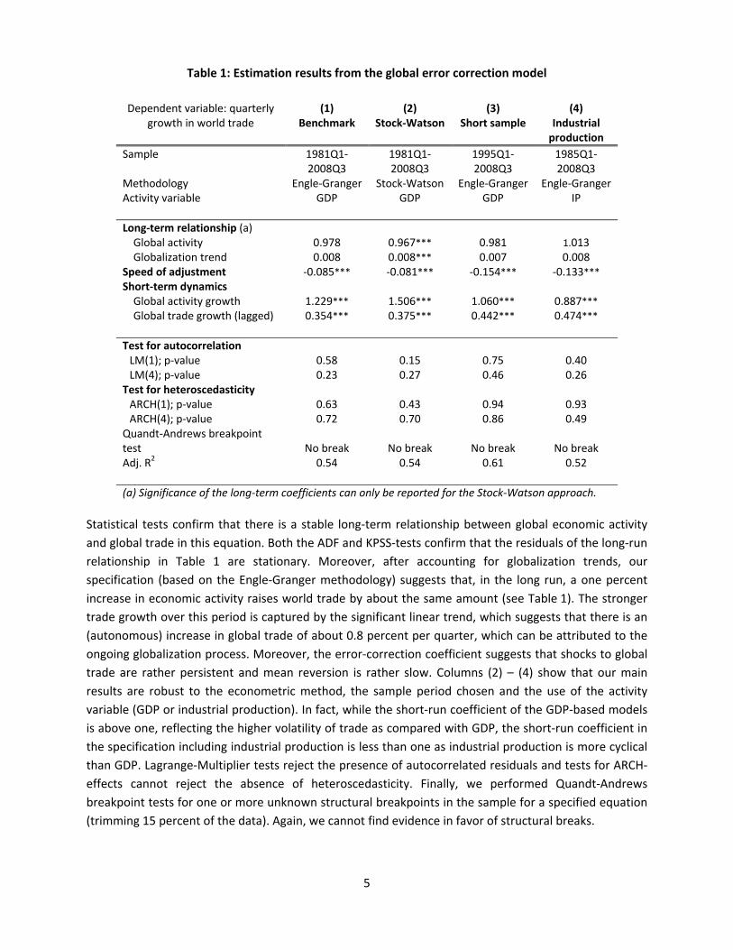
Table 1: Estimation results from the global error correction model
Dependent variable: quarterly growth in world trade
(1)Benchmark
(2)Stock‐Watson
(3)Short sample
(4) Industrial production
Sample 1981Q1‐2008Q3
1981Q1‐2008Q3
1995Q1‐2008Q3
1985Q1‐2008Q3
Methodology Engle‐Granger Stock‐Watson Engle‐Granger Engle‐GrangerActivity variable GDP GDP GDP IP
Long‐term relationship (a) Global activity 0.978 0.967*** 0.981 1.013 Globalization trend 0.008 0.008*** 0.007 0.008Speed of adjustment ‐0.085*** ‐0.081*** ‐0.154*** ‐0.133***Short‐term dynamics Global activity growth 1.229*** 1.506*** 1.060*** 0.887*** Global trade growth (lagged) 0.354*** 0.375*** 0.442*** 0.474***
Test for autocorrelation LM(1); p‐value 0.58 0.15 0.75 0.40 LM(4); p‐value 0.23 0.27 0.46 0.26 Test for heteroscedasticity ARCH(1); p‐value 0.63 0.43 0.94 0.93 ARCH(4); p‐value 0.72 0.70 0.86 0.49 Quandt‐Andrews breakpoint test No break No break No break
No break
Adj. R2 0.54 0.54 0.61 0.52
(a) Significance of the long‐term coefficients can only be reported for the Stock‐Watson approach.
Statistical tests confirm that there is a stable long‐term relationship between global economic activity
and global trade in this equation. Both the ADF and KPSS‐tests confirm that the residuals of the long‐run
relationship in Table 1 are stationary. Moreover, after accounting for globalization trends, our
specification (based on the Engle‐Granger methodology) suggests that, in the long run, a one percent
increase in economic activity raises world trade by about the same amount (see Table 1). The stronger
trade growth over this period is captured by the significant linear trend, which suggests that there is an
(autonomous) increase in global trade of about 0.8 percent per quarter, which can be attributed to the
ongoing globalization process. Moreover, the error‐correction coefficient suggests that shocks to global
trade are rather persistent and mean reversion is rather slow. Columns (2) – (4) show that our main
results are robust to the econometric method, the sample period chosen and the use of the activity
variable (GDP or industrial production). In fact, while the short‐run coefficient of the GDP‐based models
is above one, reflecting the higher volatility of trade as compared with GDP, the short‐run coefficient in
the specification including industrial production is less than one as industrial production is more cyclical
than GDP. Lagrange‐Multiplier tests reject the presence of autocorrelated residuals and tests for ARCH‐
effects cannot reject the absence of heteroscedasticity. Finally, we performed Quandt‐Andrews
breakpoint tests for one or more unknown structural breakpoints in the sample for a specified equation
(trimming 15 percent of the data). Again, we cannot find evidence in favor of structural breaks.

6
The overall fit of the relationship is also good, explaining around 50‐60 percent of the variation in global
trade. Chart 3 suggests that – based on the results reported in the first column of Table 1 – actual global
trade growth follows quite closely the growth rates projected by the model within the sample period.
However, in periods of large swings in global trade the model does not fully account for the peaks and
troughs in growth. For instance, in the early 2000s, vigorous global trade growth is only partly captured
by the model and the decline in trade in the context of the burst of the dotcom bubbles is also only
partly projected. The standard error of the regression indicates, however, that the margin of uncertainty
is non‐trivial.
Chart 3: One‐step‐ahead in‐sample forecast of world trade (quarter‐on‐quarter percentage change)
Chart 4: One‐step‐ahead forecast of world trade and actual outcomes in the midst of the crisis (quarter‐on‐quarter percentage change)
Note: The reference period is 1981‐2008. The shaded area shows the two‐standard error band.
Note: Based on the Engle‐Granger model estimated up to 2008Q3, including actual GDP realizations in the projections.
Given the strength of the collapse in global trade in 2008‐09 compared with the contraction in GDP, it is
hardly surprising that the model did not foresee the magnitude of the downturn in trade. Even if we
assume that we had perfect foresight of developments in global GDP, the model would have predicted
less than half of the actual contraction in global trade in the last quarter of 2008 and in the first quarter
of 2009 (see Chart 4), a failure shared with most standard trade models.
4. World trade at a crossroads: A scenario analysis
The Great Trade Collapse of 2008‐09 was not only hard to anticipate on the basis of standard trade
models but also poses major challenges for forecasters in the assessment of world trade going forward.
In particular, it is an open question whether the crisis will have transitory or persistent impacts on world
trade. Given that only a short period of time has gone by since the end of the downturn in global trade,
it is arguably too early to reliably detect possible structural breaks in the data associated with the global
financial crisis. Therefore, we take a different approach and use our model of world trade (see Section 3)
-2.0%
-1.0%
0.0%
1.0%
2.0%
3.0%
4.0%
5.0%
1981Q4 1985Q4 1989Q4 1993Q4 1997Q4 2001Q4 2005Q4
100
100
100
100
100
100
100
100
Actual trade
Projected trade
Standard error band
-10%
-8%
-6%
-4%
-2%
0%
2%
4%
6%
2008Q1 2008Q3 2009Q1 2009Q3 2010Q1
Model forecast Actual trade

7
as a starting point for a comprehensive scenario analysis. More specifically, we analyze in greater detail
how the shape of the recovery will look like under alternative assumptions on (i) the future profile of
world GDP, (ii) the relationship between global trade and GDP as well as (iii) the impact of renewed
financial distress.7 Before discussing each of these channels in turn, we briefly describe our baseline
scenario.
4.1 A “mechanistic” baseline scenario
In our “mechanistic” baseline
scenario, we assume that the
coefficients in our benchmark
error‐correction model in Table 1
remain unchanged and feed the
model with a plausible global GDP
profile. In more detail, we assume
– for the sake of comparability –
that world GDP growth will evolve
in line with the latest IMF
projections (World Economic
Outlook, October 2010). Following
the 0.6 percent contraction in
world GDP in 2009, the IMF expects
global economic activity to grow by
4.8 percent in 2010, 4.2 percent in
2011 and 4.5 percent in 2012 in
annual terms. Since we are mostly
interested in the overall shape of the trade recovery in the medium term, we assume that the quarterly
profile of world GDP for any given year is flat: 1.2 percent quarter‐on‐quarter throughout 2010, 1.0
percent in 2011 and 1.1 percent in 2012. Notably, these quarterly growth rates are considerably above
the average rate of 0.8 percent in our reference sample, which implies that the excess capacity in the
global economy is gradually (and partially) absorbed over this period (see Table A.2 in the appendix).
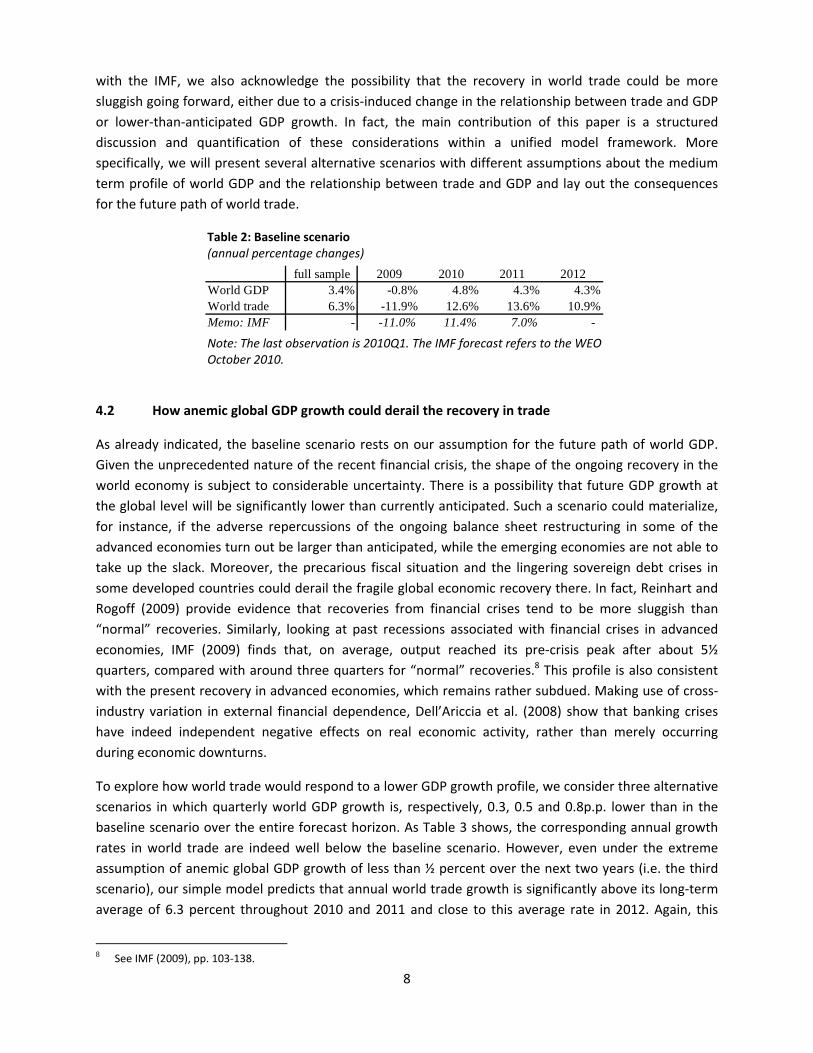
Taking our assumptions on the future path of world GDP as given, our benchmark model suggests a
strong recovery of world trade over the entire forecast horizon (see Table 2). In terms of annual growth
rates, world trade would expand 12.6 percent in 2010, 13.6 percent in 2011 and 10.9 percent in 2012.
To a notable extent, these strong growth rates are driven by the equilibrium correction mechanism in
the model. The benchmark model interprets the huge deviation of world trade growth from its
equilibrium level in late 2008 and early 2009 as an event that will be corrected by above‐average growth
in world trade – also compared to GDP – going forward. Since the estimated speed of adjustment to
disturbances is relatively low, the adjustment process takes several years (see Chart 5).
We should emphasize that the world trade growth rates implied by this mechanistic baseline scenario
are well above those in the IMF October 2010 World Economic Outlook, particularly beyond 2010In line
7 Another possibility – not discussed in this paper – would be a structural break in the globalisation (time) trend.
Chart 5: Contributions to the one‐step‐ahead out‐of‐sample projections of the global trade model (quarter‐on‐quarter growth)
Note: The last observation is 2010Q1.
-0.12
-0.10
-0.08
-0.06
-0.04
-0.02
0.00
0.02
0.04
0.06
1
2007 2008 2009 2010 2011 2012
Residuals
Error correction
Short-term dynamics
Trade
8
with the IMF, we also acknowledge the possibility that the recovery in world trade could be more
sluggish going forward, either due to a crisis‐induced change in the relationship between trade and GDP
or lower‐than‐anticipated GDP growth. In fact, the main contribution of this paper is a structured
discussion and quantification of these considerations within a unified model framework. More
specifically, we will present several alternative scenarios with different assumptions about the medium
term profile of world GDP and the relationship between trade and GDP and lay out the consequences
for the future path of world trade.
Table 2: Baseline scenario(annual percentage changes)
Note: The last observation is 2010Q1. The IMF forecast refers to the WEO October 2010.
4.2 How anemic global GDP growth could derail the recovery in trade
As already indicated, the baseline scenario rests on our assumption for the future path of world GDP.
Given the unprecedented nature of the recent financial crisis, the shape of the ongoing recovery in the
world economy is subject to considerable uncertainty. There is a possibility that future GDP growth at
the global level will be significantly lower than currently anticipated. Such a scenario could materialize,
for instance, if the adverse repercussions of the ongoing balance sheet restructuring in some of the
advanced economies turn out be larger than anticipated, while the emerging economies are not able to
take up the slack. Moreover, the precarious fiscal situation and the lingering sovereign debt crises in
some developed countries could derail the fragile global economic recovery there. In fact, Reinhart and
Rogoff (2009) provide evidence that recoveries from financial crises tend to be more sluggish than
“normal” recoveries. Similarly, looking at past recessions associated with financial crises in advanced
economies, IMF (2009) finds that, on average, output reached its pre‐crisis peak after about 5½
quarters, compared with around three quarters for “normal” recoveries.8 This profile is also consistent
with the present recovery in advanced economies, which remains rather subdued. Making use of cross‐
industry variation in external financial dependence, Dell’Ariccia et al. (2008) show that banking crises
have indeed independent negative effects on real economic activity, rather than merely occurring
during economic downturns.
To explore how world trade would respond to a lower GDP growth profile, we consider three alternative
scenarios in which quarterly world GDP growth is, respectively, 0.3, 0.5 and 0.8p.p. lower than in the
baseline scenario over the entire forecast horizon. As Table 3 shows, the corresponding annual growth
rates in world trade are indeed well below the baseline scenario. However, even under the extreme
assumption of anemic global GDP growth of less than ½ percent over the next two years (i.e. the third
scenario), our simple model predicts that annual world trade growth is significantly above its long‐term
average of 6.3 percent throughout 2010 and 2011 and close to this average rate in 2012. Again, this
8 See IMF (2009), pp. 103‐138.
full sample 2009 2010 2011 2012World GDP 3.4% -0.8% 4.8% 4.3% 4.3%World trade 6.3% -11.9% 12.6% 13.6% 10.9%Memo: IMF - -11.0% 11.4% 7.0% -

9
reflects the strong impact of the error‐correction mechanism implemented in the model. In the
following, we explore this issue in greater detail.
Table 3: World trade growth under alternative assumptions on world GDP growth (annual percentage growth)
Note: The last observation is 2010Q1. The IMF forecast refers to the WEO October 2010.
4.3 Impacts of changes in the relationship between world trade and world GDP
So far, we have implicitly assumed that, in the absence of renewed disturbances, world trade will
gradually return to levels consistent with its long‐run equilibrium relationship with global GDP. In other
words, we assumed that the crisis had only transitory effects that are unwinding over the horizon.
Moreover, we have taken for granted that the post‐crisis equilibrium relationship will be the same as
that observed before the crisis. In the following, we relax these assumptions and analyze the
consequences for the future path of world trade.
The recovery in global trade observed in the second half of 2009 and the first half of 2010 indeed
suggests that a significant part of the trade downturn in the crisis was transitory and has been
unwinding.9 In particular, the inventory dynamics magnified both the downturn and the subsequent
upturn in global trade (see Alessandria et al. 2010). This is also in line with the argument that the global
financial crisis led to a drop in demand for intermediate inputs, which explains the sharp fall in global
trade (see Bems et al. 2010). In mid‐2010, however, inventories have been approaching levels in line
with historical averages, which implies that the restocking is likely to have a less pronounced effect in
the period ahead. The same argument holds for the possible disruption of global supply chains.10
Moreover, the strength of the trade recovery in this period was also supported by factors that were
themselves transitory. Most notably, fiscal stimulus measures such as the car scrapping schemes
provided strong support to global trade.11 Given the need to retrain public finances, however, support
from these measures is also receding.
9 See ECB (2010) for an overview of the different factors shaping the downturn and the subsequent recovery in world trade. 10 See Di Giovanni and Levchenko (2009) for evidence on how the shock was transmitted via international production
networks. See also di Giovanni and Levchenko (2010) and Levchenko et al. (2010). 11 For an overview of the recent measures to support the car industry, see D. Haugh et al. (2010).
2010 2011 2012baseline 12.6% 13.6% 10.9%y 0.3p.p. lower 12.0% 11.7% 9.2%y 0.5p.p. lower 11.6% 10.4% 8.1%y 0.8p.p. lower 10.9% 8.4% 6.4%Memo: IMF 11.4% 7.0% -

10
Other factors argue in favor of a more
permanent adverse impact of the worst
financial crisis in post‐war history on global
trade, consistent with empirical evidence
showing that imports recover only
sluggishly in countries that underwent a
financial crisis, even when conditioning on
output (e.g. IMF 2010). Firstly, Kannan
(2010) presents evidence showing that
stressed credit conditions partly explain
the fact that recoveries from financial
crises tend to be sluggish. In light of the
ongoing sovereign debt crises and the
feeble state of the banking sector in many
advanced economies, global financial
conditions are unlikely to fully return to
the levels recorded prior to the crisis in the
near term.12 International trade would be
particularly exposed to such deterioration in financial conditions, as it is generally more sensitive to
financial distress than domestic transactions (Amiti and Weinstein 2009). To some extent, this can be
explained by the higher working capital requirements and risk associated with cross‐border trade.13
Therefore, the financial crisis made the downturn particularly trade‐intensive. This might have been
amplified by a drying‐up of trade finance in the midst of the crisis (Auboin 2009, Chauffour and Farole
2009, Dorsey 2009).
Second, policymakers might increasingly succumb to protectionism and thereby lower the trade
intensity of world GDP. While protectionism has so far been contained, protectionist pressures have
surfaced amid a sluggish recovery in many advanced economies, persisting global imbalances and the
growing risk of “currency wars” (Evenett 2010, Kee et al. 2010). Evidence on the Great Depression
suggests that governments are particularly prone to protectionism if they cannot resort to alternative
expansionary policies, such as fiscal or monetary policy (Eichengreen and Irwin 2009).
Third, a shift in demand from tradable to non‐tradable goods could also be reinforced by the crisis‐
induced increase in government expenditure relative to GDP across the globe, as the latter is typically
characterized by more pronounced home bias than private absorption.
In terms of the error correction model described in Section 3, there are several ways to capture
persistent changes in the relationship between trade and GDP. In our “downward shift” scenario, we
assume that there will be no further error correction in world trade going forward. Loosely speaking, we
force the model not to interpret the remaining deviation from the long‐run relationship of world trade
and world GDP over the projection horizon as a transitory event that is to be further corrected in the
12 Banking crises like the one observed in the recent past are typically followed by other episodes of financial distress,
particularly as far as sovereign debt is concerned. See Reinhart and Rogoff (2009). 13 For more details on the time lags involved in international trade, see Djankov et al. (2006) and Hummels (2001).
Chart 6: Impacts of changes in the relationship between global trade and GDP (log scale)
Note: The last observation is 2010Q1. Projections up to 2012Q4.
4.8
4.9
5.0
5.1
5.2
5.3
5.4
2005 2006 2007 2008 2009 2010 2011 2012
TradeBaseline"Downward shift""New normal"

11
subsequent quarters. As a consequence, there is a permanent one‐off downward shift in the level of
trade. Technically speaking, we set the residuals from the first‐step Engle‐Granger equation to zero from
2010Q2 onwards. Under this scenario, the projected profile for world trade growth for 2011 would be
much lower, but still above the path projected by the IMF (see Chart 6 and Table 4).
An alternative way to model a more inward‐oriented growth profile is to assume that the elasticity of
trade to GDP would be lower than before the crisis, at least for some time. We add these alternative
elasticities to the downward shift in the level of trade implemented before and call this scenario “new
normal”. In more detail, we assume that both the short‐run elasticity 1 and the long‐run elasticity ( )
shrink by a factor of 0.8. In this case, the positive impact of an increase in world GDP on world trade is
lower than in the baseline scenario. Taking the GDP profile as given, the trajectory of world trade is now
significantly flatter than in the “downward shift” or the baseline scenario, and very close to the IMF
projection.14
Table 4: World trade growth under alternative scenarios (annual percentage growth)
Note: The IMF forecast refers to the WEO October 2010. See main text for details on the various scenarios.
At first sight, it appears that the “new normal” scenario is at odds with the data. After all, world trade
expanded rapidly in the second half of 2009 and the first half of 2010, casting doubt on the notion of
lower trade elasticities. However, structural changes in the global economy might so far have been
concealed by the countervailing impact of temporary factors, such as the inventory cycle and the
extensive fiscal stimuli across the globe. These factors may have temporarily stimulated world trade
(also by propping up world GDP), but their impacts are already waning. Indeed, world trade growth
slowed down considerably in the second half of 2010. It seems fair to conclude that the jury is still out
on this, as more sophisticated econometric analysis has to wait until a sufficient number of post‐crisis
observations become available.
Clearly, imposing a lower elasticity of trade to GDP (Section 4.3) is observationally equivalent to
assuming a lower GDP profile compared to the baseline (Section 4.2) as far as the future path of world
trade is concerned. Nevertheless, these scenarios differ with respect to the underlying rationale. More
specifically, the “new normal” scenario assumes that trade will be hit more than overall economic
activity, due to trade‐specific frictions such as an increase in protectionism. By contrast, the “lower GDP
growth” scenarios are concerned with the possibility of prolonged economic weakness in overall
economic activity, which translates “one‐to‐one” into a lower trade profile.
14 If only the long‐run elasticity changed, the discrepancy between the “downward shift” and the “new normal” scenarios
would be relatively small in the short and medium term – due to the low speed of adjustment – but increase considerably over time.
2010 2011 2012baseline 12.6% 13.6% 10.9%"downward shift" 11.7% 9.3% 8.2%"new normal" 11.2% 7.7% 6.6%Memo: IMF 11.4% 7.0% -

12
In summary, there is a possibility that the fallout of the financial crisis will affect the relationship
between international trade and economic activity, at least in the near term. Our scenario analysis
illustrates that this would dramatically alter the future path of world trade. Crucially, such a scenario has
to be imposed by the modeler, as the equilibrating forces are inherent to our error correction model. In
the following section, we develop an alternative to this approach by augmenting the model with a
financial distress variable. As a result, the model will be able to generate a rather sluggish recovery in
world trade without turning off the error correction mechanism.
4.4 How financial distress affects world trade
As already indicated the near‐term growth in world trade might be hindered by the fact that financial
conditions have not yet returned to pre‐crisis levels. In this section we try to account for stressed credit
conditions more explicitly. We explore the role of financial conditions in determining the future path of
world trade by augmenting the short‐term dynamics of the error correction model with a widely‐used
measure of financial distress: the Chicago Board Options Exchange Market Volatility Index (VIX). The VIX
measures the implied volatility of S&P 500 index options and is available from 1990 onwards. Spikes in
the VIX tend to coincide with periods of financial distress (see Chart 7).
Interestingly, the VIX turns out to be
insignificant when included in levels or first
differences (results not reported here). Hence,
in general, the impact of financial conditions on
world trade appears to be well‐captured by the
other variables of the model, particularly world
GDP. However, the results change notably
when we differentiate between “normal times”
and periods of severe financial distress.
Technically speaking, we construct a dummy
variable that is equal to one if the VIX deviates
significantly (i.e. one‐and‐a‐half standard
deviations) from its longer‐term mean, and zero
otherwise. This financial distress dummy turns
out to be statistically significant and has a
negative sign, as expected (see Table 5, third
column). The estimated coefficient is relatively
small, with quarterly world trade growth being
around 1p.p. lower in periods of financial
distress as compared to “normal” times, ceteris
paribus. This is equivalent to about one standard deviation of world trade growth. However, one should
bear in mind that the dummy captures the effects of financial distress on world trade over and above
those already captured by the other variables, particularly world GDP and the history of world trade
itself. In other words, our results indicate that severe financial distress has a significant effect on world
trade growth, over and above its indirect impact through GDP. Moreover, episodes of severe financial
distress may last more than one quarter, in which case the estimated impact has to be cumulated.
Chart 7: Financial distress indicators
(VIX, global crisis index, Ted spread)
Sources: Bloomberg, Laeven and Valencia (2010) and IMF.
Note: The global “crisis index” is a GDP‐weighted index of
financial crises in individual countries. The crisis episodes
are taken from Laeven and Valencia (2010) and the GDP
weights from the IMF‐WEO database.
0
10
20
30
40
50
60
70
1980 1985 1990 1995 2000 2005 2010
0.0
0.5
1.0
1.5
2.0
2.5
3.0
3.5
VIX Crisis index Ted spread (rhs)

13
Table 5: The impact of financial distress – estimation results from the global error correction model
Dependent variable: quarterly growth in world trade
(1)Benchmark
(2)Short sample
(3)VIX
(4) Ted
spread
(5)Crisis index
1981Q1‐2008Q3
1990Q1‐2008Q3
1990Q1‐2008Q3
1985Q1‐2008Q3
1980Q1‐2008Q3
Long‐term relationship Global activity 0.978 0.978 0.981 0.981 0.981 Globalization trend 0.008 0.008 0.007 0.007 0.007Speed of adjustment ‐0.085*** ‐0.097*** ‐0.100*** ‐0.101*** ‐0.083***Short‐term dynamics Global activity growth 1.229*** 1.179*** 1.281*** 1.257*** 1.279*** Global trade growth (lagged) 0.354*** 0.416*** 0.384*** 0.377*** 0.351***Financial distress ‐ ‐ ‐0.006* ‐0.003* ‐0.003* adj. R2 0.54 0.56 0.59 0.53 0.55
To illustrate the impacts of renewed financial distress on the future path of world trade, we consider a
scenario in which financial conditions remain strained over the entire forecast horizon. More
specifically, we feed the estimated model (see Table 5, column 3) with a financial distress dummy that is
equal to unity from 2010Q2 onwards. Unfortunately, our simple model does not allow us to capture
interactions between financial distress and GDP growth, since both variables are treated as exogenous.
Therefore, we make the additional (and admittedly ad‐hoc) assumption that financial distress will be
associated with a 0.8 p.p. reduction in GDP growth over the horizon compared to the baseline (as in
Section 4.2). The corresponding path of world trade is well below the baseline (see Chart 8). At the end
of the forecast horizon, trade is 12 percent lower than it would have been in the baseline scenario with
benign financial conditions. Even if we assume that GDP growth remains unchanged with respect to the
baseline, annual world trade growth would be around one percentage point lower than in the baseline
in both 2011 and 2012.

14
Obviously, it is not straightforward to
capture the “global financial conditions”
with a single variable. To check for the
robustness of our results, we have
therefore considered alternative measures
of financial conditions, including the Ted
spread and a GDP‐weighted index of
financial crises. The key finding remains
that these financial variables are
insignificant when included in non‐binary
form, but turn out to be significant as a
dummy variable (see Table 5, columns 4
and 5).
5. An examination of U.S. exports
Having discussed the outlook for global trade, we now examine the performance of and prospects for
U.S. exports. Our interest in the U.S. is twofold. First, given the United States weight in global trade,
developments in U.S. exports are clearly an important driver of aggregate trade volumes. Second,
focusing on a single country allows for an examination of bilateral trade relationships that is not possible
when considering aggregates.
5.1 An error correction model for U.S. exports
What do the scenarios for world trade outlined above imply for the trajectory of U.S. exports? In order
to assess the impact of the various global trade scenarios on U.S. exports we first construct a baseline
model that mimics the structure of the global error correction model outlined earlier.
The global model was modified along two key dimensions. First, a trade‐weighted measure of the real
exchange rate was included as an independent variable in the U.S. model. In the global model, relative
price changes could be ignored, as they would be expected to change the cross‐country pattern of trade
but leave the aggregate volume of trade unaffected. However, when considering U.S. exports
separately, relative prices play a potentially important role in explaining both the long‐run equilibrium
level of exports as well as the short‐term dynamics. Second, attempts to include a trend were met with
counterintuitive results and hence the trend term was dropped from the estimation. (The estimated
trend was negative with the effect of blowing up the income elasticity.)
The estimated parameters of the U.S. model are presented in Table 6. The estimated long‐run income
elasticity is in the vicinity of 1½, greater than that in the global model, but in line with other models of
U.S. exports (including the Federal Reserve’s U.S. International Transactions model). The real exchange
Chart 8: The impacts of financial distress (log scale)
Note: The last observation is 2010Q1. Projections up to 2012Q4. For details see main text.
4.8
4.9
5.0
5.1
5.2
5.3
5.4
2005 2006 2007 2008 2009 2010 2011 2012
Trade"Financial distress""Baseline"

15
rate has a significant negative coefficient and is estimated to have a long lag structure, with changes in
the real exchange rate continuing to impact the level of exports for three years. Shocks to U.S. exports
are persistent, but the speed of adjustment back to equilibrium is considerably faster than that
estimated in the global model. A lagged dependent variable was included in the regression; however,
the coefficient was insignificant and is not reported. Overall the regression explains 48 percent of the
variation in U.S. exports, and hence performs on par with the global model.
Table 6: Estimation results from the U.S. exports error correction model
Dependent variable: quarterly growth in U.S. real exports of goods*
Benchmark
Sample 1981Q1‐2008Q3Methodology Engle‐Granger
Activity variable Export –Weighted Foreign
GDP
Long‐term relationship (a) Global activity 1.474 Real exchange rate: sum(0 to ‐12) ‐0.725Speed of adjustment ‐0.193***Short‐term dynamics Lagged global activity growth 1.755*** Real exchange rate: sum(0 to ‐12) ‐0.772***
Test for autocorrelation LM(1); p‐value 0.73 LM(4); p‐value 0.45Test for heteroscedasticity ARCH(1); p‐value 0.28 ARCH(4); p‐value 0.12 Adj. R2 0.48
*Goods excluding end‐use code 213 (Computers). Due to idiosyncratic price developments, real computer exports exhibit movements that are not well explained by the model determinates and obscure the overall analysis.
Projected U.S. exports from the baseline model are plotted in Chart 9, along with the model solution for
the long‐run level of exports. For the purposes of the projections the real exchange rate is assumed to
be unchanged from 2010:Q3 onward and foreign GDP expands in line with the IMF WEO forecast. As can
be seen by comparing the long‐run equilibrium with the data, a large model error opened up over the
2008‐09 period, such that even given the decline in foreign GDP, U.S. exports appeared exceptionally
weak. By the third quarter of 2010, the error had closed a bit from the mid‐2009 trough, but the gap
remains substantial. The “baseline” forecast, indicated by the dashed‐circle line, calls for the rapid
expansion of exports over the next two years, boosted importantly by the model’s error correction
mechanism..
The chart also plots the “downward shift” and “new normal” scenarios discussed previously. In the
“downward shift” scenario it is assumed that there is no further error correction in exports, such that

16
the gap between level of exports in the third quarter of 2010 and the estimated long‐run equilibrium
level remains constant. Under this scenario, export growth in the projection is determined only by the
path of foreign GDP growth and the lagged effect of previous exchange rate changes. The “new normal”
scenario maintains the no further bounce back assumption of the “downward shift” scenario, but also
assumes a 20 percent decline in the foreign income elasticity of exports going forward.
Chart 9: Baseline Projection and Alternative Scenarios: 2010Q4 – 2012Q4
A comparison of projected export growth rates is presented in Table 7. As can be seen by comparing the
“baseline” forecast with the “downward shift” scenario, the assumption of further export bounce back
in the baseline is adding almost 2½ percentage points to export growth in 2011 and over 1 percentage
point in 2012. Thus, the prospect of further bounce back and whether or not it materializes is central to
any near‐term and medium‐term forecast for U.S. export growth. Giving the importance of bounce back,
the lower income elasticity assumed in the “new normal” scenario is second‐order in the near‐term,
although would be of increasing importance going forward.
Table 7: U.S. Export Growth under Alternative Scenarios
2010 2011 2012
Baseline 8.7 9.5 8.6
“Downward Shift” 7.5 7.1 7.4
“New Normal” 7.5 6.1 6.9
700
800
900
1,000
1,100
1,200
1,300
2005 2006 2007 2008 2009 2010 2011 2012
Long-Run Model BaselineDownward Shift New NormalData
Bill
ion
s o
f 2
00
5 U
SD

17
5.2 U.S. exports by destination and the impact of a multi‐speed recovery
One of the advantages of examining U.S. trade as opposed to world trade is the ability to focus on
bilateral trading relationships. In this section we consider U.S. exports by destination disaggregated
across advanced foreign economies (AFEs) and emerging market economies (EMEs). This disaggregation
will allow two further avenues for examining the prospects for U.S. exports. First, we can decompose
the model error into components due to trade with the AFEs and EMEs. Since, as outlined earlier, the
prospect for further bounce back is key to the outlook for U.S. export growth; insight into the
distribution of the error can provide important information as to whether bounce back will actually
materialize. Second, given that the pace of EME growth is expected to far exceed AFE growth over the
next few years, a forecast embodied in the IMF WEO projection, we can examine the implications of the
projected multi‐speed recovery for U.S. exports.
We estimate separate error‐correction models for U.S. exports to AFE and EME country groupings. The
models are similar in structure to that estimated for aggregate exports. For each country group, the
dependent variable is the growth rate of real goods exports from the U.S. to that country group and the
independent variables are export‐weighted GDP and real exchange rates calculated within each
grouping. The results of the regressions are reported in Table 8. A few notable differences are apparent
across the two regions. First, the advanced economies have a higher income elasticity but lower price
elasticity for U.S. exports compared with the emerging market economies. Second, exports to the
emerging market economies tend to bounce back more quickly to their long‐run equilibrium than
exports to the advanced economies.
Table 8: Estimation results from the U.S. exports error correction model – Disaggregated markets
Dependent variable: quarterly growth in U.S. real exports
(1)AFEs
(2)EMEs
Sample 1981Q1‐2008Q3
1981Q1‐2008Q3
Long‐term relationship GDP 1.656 1.335 Real Exchange Rate (0 to ‐12) ‐0.484 ‐0.904Speed of adjustment ‐0.148*** ‐0.244*** Short‐term dynamics Lagged GDP growth 2.169*** 1.538*** Real Exchange Rate (0 to ‐12) ‐0.437*** ‐1.507*** adj. R2 0.36 0.33
Having estimated separate trade models for the AFE and EME countries, we can forecast exports to the
two country groupings independently. Before looking at the implications of the disaggregated forecasts
for the U.S. export outlook, it is instructive to use the model forecast to examine the 2008‐09 trade
collapse and the current state of the bounce back in exports. The disaggregated models allow us to
decompose the deviation between actual exports and the model‐predicted long‐run equilibrium
(apparent in Chart 9) into components due to underperformance of exports to the AFEs and EMEs
separately. As shown in Chart 10, the collapse in exports in 2008‐09 resulted in roughly equal model

18
errors for the AFEs and EMEs, with exports underperforming relative to GDP by about the same amount
in both regions. The model errors in both regions decreased through the second half of 2009, as exports
to both regions bounced back; however, exports to the EME countries appear to have retraced slightly
more of their unexplained weakness. So far through 2010, neither the AFE nor the EME model errors has
closed much further, and exports have remained weak relative to GDP in both markets. This does not
necessarily imply a loss in U.S. export market share, as it may partly reflect a change in the elasticity of
trade to GDP across all exporters worldwide, as discussed in Section 4. The model‐implied weakness of
exports to the EMEs may come as a surprise given the strong growth of apparent exports to the region
over 2010; however, EME GDP growth has also been robust over the period and the model would have
had exports increase by an even greater amount than was realized.
What does the error decomposition in Chart 10 tell us regarding the prospects for continued error
correction in U.S. exports? The relative importance of the AFE countries in the continued
underperformance of U.S. exports is not surprising given that a number of trading partners in this
grouping suffered severe financial crises. As noted earlier, empirical evidence points to only a sluggish
recovery of imports in countries impacted by financial crisis (IMF 2010). It therefore seems likely that
this residual may persist for some time. The persistence of the EME model error is harder to explain, in
that countries in this grouping largely avoided the financial crisis and have had robust recoveries in GDP.
It could be that GDP growth in these countries has been boosted largely by sectors that are less import
intensive, i.e. government spending and infrastructure, and as such the model, ignorant of the source of
GDP growth, is disappointed by the relative paucity of imports drawn in by such growth. As the impact
of fiscal stimulus fades and increased government spending is replaced by other components of GDP, it
is likely that imports will recover, pushing U.S. exports to the region closer in line with the level of GDP.
However, the persistent gap between actual exports and their estimated equilibrium level might also
partly reflect a change in the relationship of trade to GDP, as discussed in Section 4.
A disaggregated consideration of AFE and EME exports also allows us to examine the likely impact of the
multi‐speed recovery embodied in the IMF’s outlook for world growth. In the October 2010 WEO the
IMF projects that advanced economies will grow at a sluggish 0.5 percent quarter‐on‐quarter pace in
2011, picking up a bit to 0.7 percent in 2012. In contrast, emerging market economies are projected to
expand at a robust 1.6 percent rate through 2011 and 2012. Using the IMF’s growth projections and
keeping the real exchange rate flat for both AFEs and EMEs, we are able to project U.S. exports to each
region separately, and then aggregate up to a forecast for total U.S. export growth. As shown in Table 9,
it turns out that the multi‐speed recovery has only a small impact on the forecast in comparison with the
baseline aggregate model considered in the previous section.

19
Chart 10: Decomposition of U.S. export model error across destination markets
The relatively muted impact of the multi‐speed recovery on projected export growth is a result of two
factors. First, the AFEs and EMEs each accounted for roughly half of U.S. exports and half of global
output in the third quarter of 2010. Thus, from a weighting perspective it makes little difference if we
consider global GDP growth or disaggregated growth. Second, the higher growth rate of the EME
economies is almost balanced by their lower estimated income elasticity and vice versa for the AFE
economies, as such that there is little net impact on the projection for export growth.
Another scenario the disaggregated models allow us to consider is a multi‐speed adjustment back to
long‐run equilibrium. Given that the financial crisis has been centered in the AFEs, it is possible that U.S.
exports to the region will remain below their long‐run equilibrium for an extended period of time. The
“prolonged AFE weakness” scenario then is one where there is no further error correction on the part of
exports to the AFEs while exports to the EMEs are allowed to bounce back in line with the model. As
shown in Table 9, the lack of bounce back in the AFEs lowers projected export growth by 1 percentage
point in 2011 and 0.6 percentage point in 2012.
Table 9: U.S. export growth with a multi‐speed recovery
2010 2011 2012
Aggregate Baseline 8.7 9.5 8.6
“Multi‐speed recovery” 8.6 9.8 9.0
“Prolonged AFE weakness” 8.3 8.8 8.4
-160
-140
-120
-100
-80
-60
-40
-20
0
20
I II III IV I II III IV I II III
2008 2009 2010
Advanced Foreign EconomiesEmerging Market Economies
Bill
ion
s o
f 2
00
5 U
SD

20
5.3 U.S. exports by commodity
Having considered disaggregated markets, we now turn to an examination of U.S. exports of
disaggregated commodities. By separately modeling U.S. exports by category of good we can take
another cut at examining the weakness of exports through 2008‐09 and the prospects for growth going
forward.
We estimated error correction models of the same style as in the previous two sections for a
comprehensive breakdown of exports into six major commodity headings. For each regression the
independent variables, GDP and the real exchange rate, are identical to the series used in the aggregate
regression in Table 6. As can be seen in Table 10, there is considerable variation in the income and price
elasticity of exports across commodities. Exports of capital goods show the greatest price sensitivity,
while food and “other” goods are relatively price inelastic. Consumer goods are the most income
elastic, while exports of foods and “other” goods (importantly military goods) are less sensitive to
changes in income.
On the surface, the higher income elasticity of consumer goods may appear surprising given that
consumption, particularly of non‐durables, is generally less cyclical than investment. In part, this
surprising result is likely the outcome of the specific composition of U.S. exports of consumer goods. For
example in the second quarter of 2008, fully 20 percent of U.S. real consumer goods exports consisted
of artwork, jewellery, and gemstones, probably exceeding the weight on such goods in all but a few
consumption bundles. More surprising given the high estimated income elasticity, is that
pharmaceuticals comprised roughly a quarter of U.S. consumer goods exports, and it seems likely that
such exports would be particularly income inelastic.15
Table 10: Estimation results from the U.S. exports error correction model – Disaggregated commodities
Dependent variable: quarterly growth in U.S. real exports
(1)Food
(2)Industrial Materials
(3)Capital Goods
(4)Autos
(5) Consumer Goods
(6)Other
Sample 1995Q2‐2008Q3
1995Q2‐2008Q3
1995Q2‐2008Q3
1995Q2‐2008Q3
1995Q2‐2008Q3
1995Q2‐2008Q3
Long‐term relationship Global GDP 0.772 1.316 1.480 1.615 2.105 0.885 Real exchange rate: Sum(0 to ‐12) ‐0.318 ‐0.504 ‐0.889 ‐0.715 ‐0.766 0.0254Speed of adjustment ‐0.431*** ‐0.315*** ‐0.183*** ‐0.754*** ‐0.319*** ‐0.446***Short‐term dynamics Lagged global growth 0.324 1.219*** 1.770*** 1.964*** 1.813*** 1.332*** Real exchange rate: Sum(0 to ‐12) 0.114 ‐0.295 ‐.187 ‐0.345 ‐0.783*** 2.934*** adj. R2 0.18 0.26 0.33 0.42 0.32 0.20
15 In fact, looking just at the most recent downturn and rebound in exports, the greatest volatility in consumer goods exports was
recorded in the “gem diamonds” category which plunged 50 percent from the second quarter of 2008 through the second quarter of 2009 only to then rebound 50 percent through the third quarter of 2010. In contrast, exports of pharmaceuticals actually increased 25 percent during the downturn in trade and have fallen back a bit during the rebound.
21
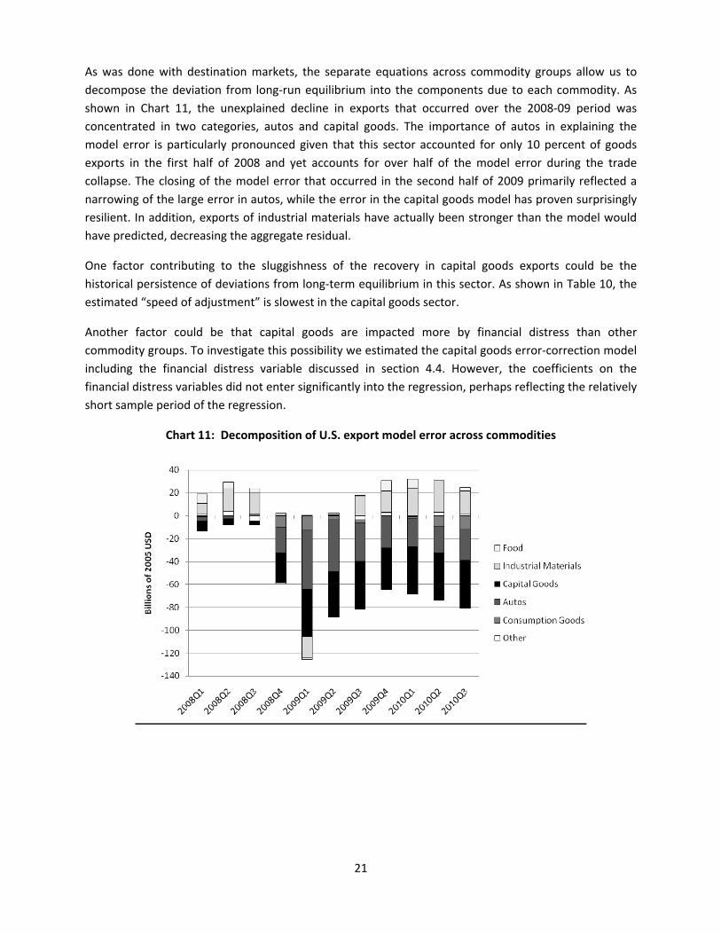
As was done with destination markets, the separate equations across commodity groups allow us to
decompose the deviation from long‐run equilibrium into the components due to each commodity. As
shown in Chart 11, the unexplained decline in exports that occurred over the 2008‐09 period was
concentrated in two categories, autos and capital goods. The importance of autos in explaining the
model error is particularly pronounced given that this sector accounted for only 10 percent of goods
exports in the first half of 2008 and yet accounts for over half of the model error during the trade
collapse. The closing of the model error that occurred in the second half of 2009 primarily reflected a
narrowing of the large error in autos, while the error in the capital goods model has proven surprisingly
resilient. In addition, exports of industrial materials have actually been stronger than the model would
have predicted, decreasing the aggregate residual.
One factor contributing to the sluggishness of the recovery in capital goods exports could be the
historical persistence of deviations from long‐term equilibrium in this sector. As shown in Table 10, the
estimated “speed of adjustment” is slowest in the capital goods sector.
Another factor could be that capital goods are impacted more by financial distress than other
commodity groups. To investigate this possibility we estimated the capital goods error‐correction model
including the financial distress variable discussed in section 4.4. However, the coefficients on the
financial distress variables did not enter significantly into the regression, perhaps reflecting the relatively
short sample period of the regression.
Chart 11: Decomposition of U.S. export model error across commodities

22
6. Conclusions
Our analysis suggests that during the crisis both world trade and U.S. exports declined significantly more
than would have been expected on the basis of historical relationships with economic activity.
Moreover, this gap between actual and equilibrium trade is closing only slowly and, under reasonable
assumptions, could persist for some time to come. Our analysis highlights that in assessing the near‐
and medium‐term outlook for trade, both globally and for the U.S. specifically, assumptions regarding
the speed and degree to which the gap between actual and equilibrium trade closes are absolutely
central to any projection for trade going forward. It is too soon to say with any certainty whether the
crisis will have only transitory or persistent effects on the relationship between trade and economic
activity. However, we have constructed plausible scenarios through which the impact on trade is both
long‐lasting and meaningful.
Our analysis has shown that many of the factors shaping the future path of world trade will affect U.S.
exports in a similar fashion. However, it is also clear that world trade and U.S. trade are highly
interdependent (di Mauro et al. 2010). While these linkages are not endogenous to our models, some of
the scenarios discussed in this paper can nevertheless be interpreted along these lines. For instance, the
scenario with lower world GDP growth (Section 4.2) could partly reflect lower activity growth in the U.S.
Of course, the interdependency also works in the other direction. For instance, a possible break in the
elasticity of world imports to GDP might further complicate the task of forecasting U.S. exports on the
basis of foreign GDP.
23
References
G. Alessandria, J. Kaboski and V. Midrigam, ”The Great Trade Collapse of 2008‐09: An Inventory
Adjustment?”, NBER Working Paper 16059, 2010.
M. Amiti and D. Weinstein, “Exports and financial shocks”, NBER Working Paper No. 15556, 2009.
M. Auboin, “Boosting the availability of trade finance in the current crisis: Background analysis for a
substantial G20 package”, CEPR Policy Insight No 35, 2009.
M. Bussière and B. Schnatz, “Evaluating China’s Integration in World Trade: A Benchmark Based on a
Gravity Model”, Open Economies Review, 2009, Vol. 20, No. 1, pp. 85‐111, 2009.
R. Bems, R. C. Johnson and K.‐M. Yi, ”Demand Spillovers and the Collapse of Trade in the Global
Recession”, IMF Working Papers 10/142, International Monetary Fund, 2010.
J.‐P. Chauffour and T. Farole, “Trade finance in crisis: market adjustment or market failure?”, Policy
Research Working Paper No 5003, The World Bank, 2009.
C. Cheung and S. Guichard, “Understanding the World Trade Collapse”, OECD Working Papers, No. 729,
2009.
G. Dell’Ariccia, E. Detragiache and R. Rajan, “The real effects of banking crises”, Journal of Financial
Intermediation, Vol. 17, pp. 89‐112, 2008.
J. di Giovanni and A. Levchenko, “Putting the parts together: Trade, vertical linkages, and business cycle
comovement”, American Economic Journal, Vol.2, Issue 2, 2010.
J. di Giovanni and A. Levchenko, ”International Trade and Aggregate Fluctuations in Granular
Economies”, Working Papers 585, University of Michigan, 2009.
F. di Mauro, S. Dées and M. Lombardi, “Catching the flu from the United States. Synchronisation and
transmission mechanisms to the euro area”, Palgrave Macmillan, 2010.
T. Dorsey, “Trade finance stumbles”, Finance and Development, Vol. 46, No 1, March 2009.
S. Djankov, C. Freund and C. Pham, “Trading on time”, Policy Research Working Paper No 3909, The
World Bank, 2006.
B. Eichengreen and D. Irwin, “The slide to protectionism in the Great Depression: Who succumbed and
why?”, Working Paper No. 15142, NBER, 2009.
C. Engel and J. Wang, “International trade in durable goods: Understanding volatility, cyclicality, and
elasticities”, NBER Working Paper No. 13814, 2008.
European Central Bank, “Recent developments in global and euro area trade”, article in the ECB Monthly
Bulletin, August 2010.
S. Evenett (ed.), “Tensions contained… for now: The 8th GTA Report”, CEPR, November 2010.

24
C. Freund, “The Trade Response to Global Downturns – Historical Evidence”, World Bank Policy Research
Paper, No. 5015, 2009.
D. Haugh, A. Mourougane and O. Chatal, “The automobile industry in and beyond the crisis”, Economics
Department Working Papers, No 745, OECD, 2010.
D. Hummels, “Time as a trade barrier”, GTAP Working Paper Series, No 18, 2001.
D. Hummels, J. Ishii and K.‐M. Yi, “The nature and growth of vertical specialization in world trade”,
Journal of International Economics, Vol. 54, Issue 1, 2001.
International Monetary Fund, “World Economic Outlook”, October 2010.
International Monetary Fund, “World Economic Outlook”, April 2009.
P. Kannan, “Credit conditions and recoveries from recessions associated with financial crises”, IMF
Working Paper, No. 83, 2010.
H. Kee, C. Neagu and A. Nicita, “Is protectionism on the rise? Assessing national trade policies during the
crisis of 2008”, Policy Research Working Paper No. 5274, The World Bank, 2010.
J. Kleinert and N. Zorell (2010), „The export magnification effect of offshoring”, IAW Discussion Papers,
No. 63.
A. Levchenko, L. Lewis and L. Tesar, “The collapse of international trade during the 2008‐2009 crisis: In
search of the smoking gun”, Working Paper No 16006, NBER, 2010.
G. Maddala and I. Kim, “Unit roots, cointegration, and structural change”, Cambridge University Press,
2003.
C. Reinhart and K. Rogoff, “This time is different: Eight centuries of financial folly”, Princeton University
Press, 2009.
J. Wang, “Durable goods and the collapse of global trade”, Economic Letter, Vol. 5, No 2, Federal
Reserve Bank of Dallas, 2010.

25
Appendix
Table A.1: International trade in goods during the recent episode (percentage changes)
Note: The country‐specific peaks and troughs are based on the period 2008‐09. The underlying
data are seasonally adjusted and transformed into three‐month‐moving averages. Aggregates
include intra‐regional trade.
Sources: CPB and ECB staff calculations.
Table A.2: Descriptive statistics (based on quarterly percentage growth rates)
Note: "Full sample" refers to 1980Q1‐2008Q3.
Exports Imports
peak to
trough
trough to
Sep-10
peak to
Sep-10
peak to
trough
trough to
Sep-10
peak to
Sep-10
W ORLD -18.5 21.6 -0.9 -20.0 22.2 -2.2
Advanced economies -21.2 18.2 -6.9 -21.8 17.2 -8.3
Euro area -20.8 15.3 -8.7 -19.5 11.7 -10.1
US -22.2 21.0 -6.0 -24.1 25.3 -4.9
Japan -39.5 53.1 -7.4 -22.0 25.3 -2.2
Emerging economies -16.1 26.7 6.3 -20.8 35.0 6.9
Asia -17.5 30.7 7.9 -23.0 45.4 12.0
China (1) -18.2 37.2 12.2 -29.4 62.0 14.4
CIS -20.3 4.6 -16.7 -34.3 31.3 -13.8
Latin America -12.4 22.8 7.6 -27.0 41.0 3.0
Brazil -21.5 43.0 12.3 -30.0 61.1 12.7
Mexico -16.2 25.4 5.2 -29.9 33.1 -6.7
MENA & SSA -16.5 19.7 -0.1 -16.3 10.2 -7.7
(1) "China" includes Hong Kong.
80s 90s2000s (up to
2008Q3)2000s (up to
2010Q1)full sample
y Mean 0.8 0.7 0.9 0.8 0.8 Median 0.8 0.8 1.1 1.0 0.9 Std. Dev. 0.3 0.3 0.4 0.6 0.3 Observations 38 40 35 41 113
m Mean 1.4 1.7 1.6 1.2 1.5 Median 1.3 1.7 2.0 2.0 1.7 Std. Dev. 0.8 0.8 1.3 2.5 1.0 Observations 35 40 35 41 110
m/y (*)1.7 2.2 1.7 1.4 1.9
Correlation 0.65 0.59 0.75 0.91 0.65