When States Get Excited or a Short Guide to time ...th.fhi-berlin.mpg.de/th/Meetings/FHImd2003/Dtalks/FHI-WS...Lecture 17th † When States Get Excited -or- a Short Guide to TDDFT

Lecture 17th • When States Get Excited -or- a Short Guide to TDDFT • Krzysztof TatarczykApplications of DFT...• Fritz-Haber-Institut, Berlin, 21-30 July, 2003

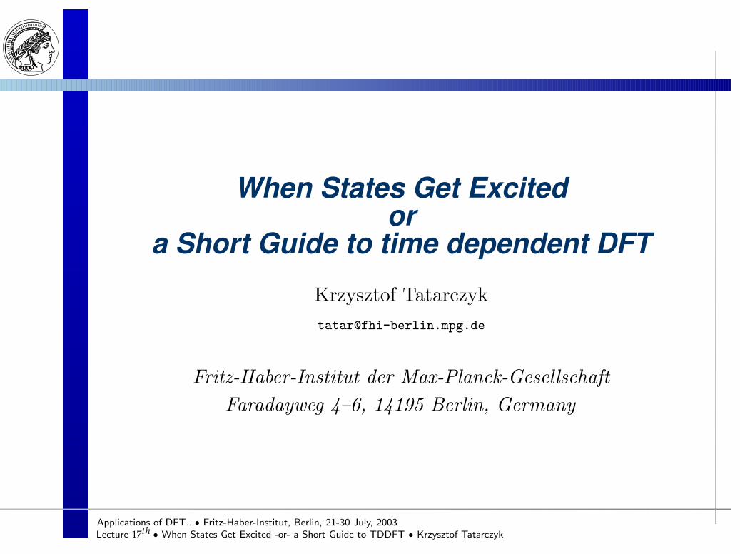
When States Get Excitedor

a Short Guide to time dependent DFT

Krzysztof Tatarczyk

[email protected]

Fritz-Haber-Institut der Max-Planck-Gesellschaft

Faradayweg 4–6, 14195 Berlin, Germany


Why study excited states ?

o Because they are there

o Motivation from experiments ⇒ progress in spectroscopymethods Example → Aluminum bulk

• Electron Energy LossSpectroscopy (EELS)

• Plasmon excitationsin bulk systems

• S(q, ω) = −q2=ε−1(q, ω)

• Anormalous behaviour ?P.M. Platzman et al., PRB 46,12 943(1992)

• Property of the materialA. Fleszar et al., PRL, 74, 590(1995)

Atomistic studies needed!

o The ultimate gainÃ more realistic description of exchange andcorrelation effects


How about surfaces ?

ë Sample EELS for a surface

4 Apart from the bulk plasmonthere exist two additional

4 The monopole surface plasmonωs due to the surface

4 The multipole surface plasmonωm due to diluted density profile

î

ë Photoemission Spectroscopy (PY)

4 The light usually excites onlythe multipole plasmon

4 features A & B ?P Detailed theoretical study desperately wanted P


Spectroscopies ?

ý Prototype Spectroscopy Measurements

q Absorption

O Electron-hole pair is createdO Charge-neutral excitation resultsO Number of electrons unchanged

q Photoemission Spectroscopy (PE)

O Electron is removed/added to the systemO Direct Photoemission scans occupied levelsO Inverse Photoemission probes unoccupied states

P I can’t directly use my ground-state code P


Kohn-Sham eigenvalues dilemma (?)

o Description of such measurements is intimately bound to theone-particle/-like energies

o These can be obtained from DFT, but...[

− 12∇

2 + Vext(r) + VH(r) + Vxc(r)]

φi(r) = ε iφi(r)

n(r) = ∑i fi|φi(r)|2 E0 = minEtot[n]

o Means ???n Static approach to many-body problem

n By design describes the ground-state properties

n Kohn-Sham eigenvalues aquire meaning via Janak theoremεi =

δE0[n]δ fiÃ all but the highest occupied one are mathematical

artifacts of the method

n the highest occupied KS eigenvalue corresponds to chemicalpotential of the system


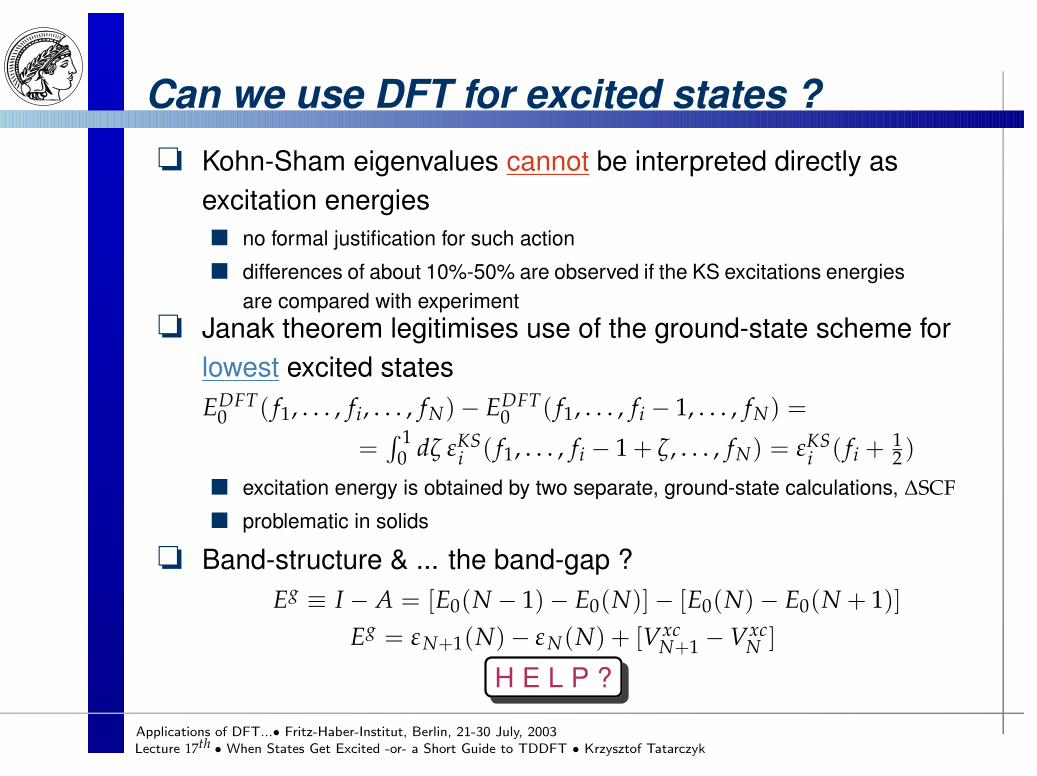
Can we use DFT for excited states ?

o Kohn-Sham eigenvalues cannot be interpreted directly asexcitation energiesn no formal justification for such action

n differences of about 10%-50% are observed if the KS excitations energiesare compared with experiment

o Janak theorem legitimises use of the ground-state scheme forlowest excited statesEDFT

0 ( f1, . . . , fi, . . . , fN) − EDFT0 ( f1, . . . , fi − 1, . . . , fN) =

=∫ 1

0 dζ εKSi ( f1, . . . , fi − 1 + ζ, . . . , fN) = εKS

i ( fi + 12 )

n excitation energy is obtained by two separate, ground-state calculations, ∆SCF

n problematic in solids

o Band-structure & ... the band-gap ?Eg ≡ I − A = [E0(N − 1) − E0(N)] − [E0(N) − E0(N + 1)]

Eg = εN+1(N) − εN(N) + [VxcN+1 − Vxc

N ]

H E L P ?


Ways to go...

In order to obtain excitation energies:

o Improve description of the bandstructuren in a way that it yields electron addition/removal energies seen in

spectroscopy experiments

n Means ? Solve the band-gap problem!F Employ the Many-Body Perturbation Theory (MBPT)

[

− 12∇

2 + VH(r)]

φi(r) +∫

d3r′ ∑(r, r′, εQPi )φi(r′) = εQP

i φi(r)

Ã Effective quasiparticle Hamiltonian with the optical mass(self-energy) operator → the GW method

F Stay within the DFT and improve the XC potential

Vx =δEx

δn

∣

∣

∣

∣

n=n0

, Ex = −12 ∑

i,j

∫

d3r d3r′φ∗i (r)φ∗

j (r′)v(r − r′)φi(r)φj(r′) Ã

the EXX method → it works (!)o How about charge-neutral excitations ?


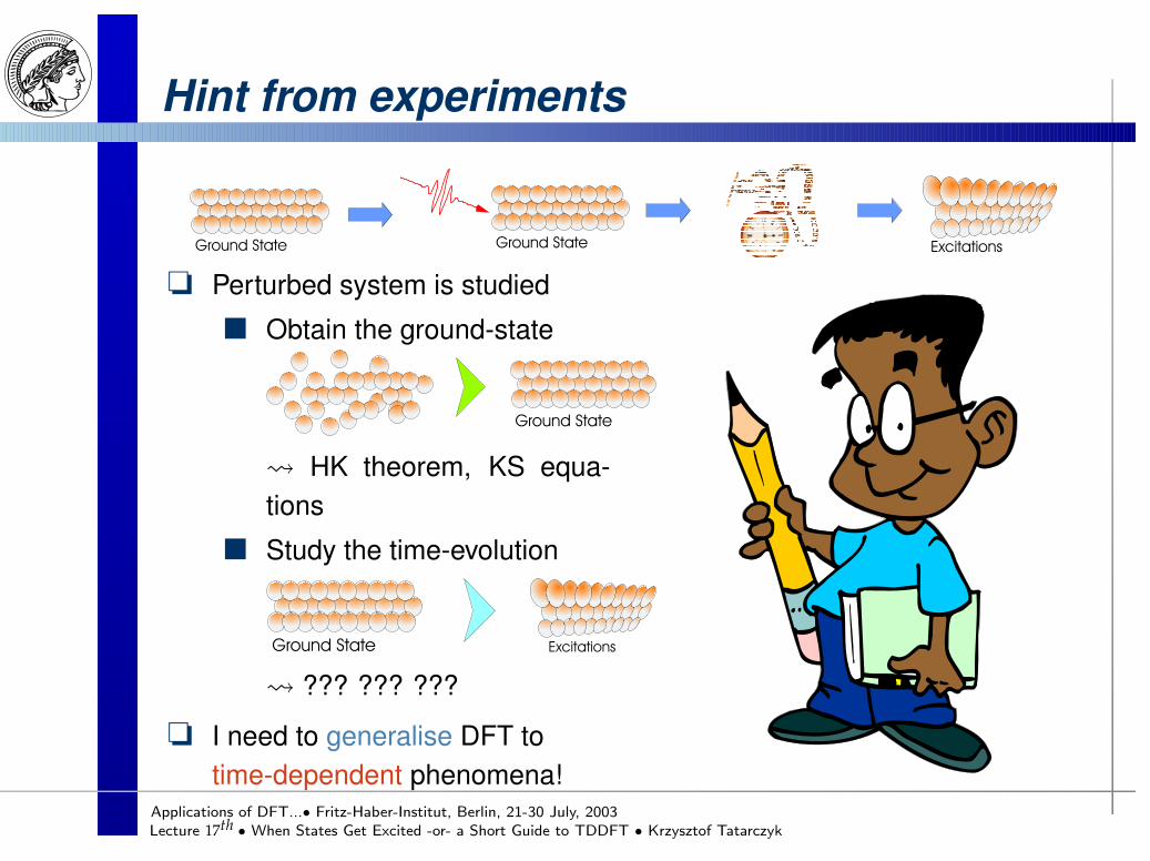
Hint from experiments

o Perturbed system is studied

n Obtain the ground-state

Ã HK theorem, KS equa-tions

n Study the time-evolution

Ã ??? ??? ???

o I need to generalise DFT totime-dependent phenomena!


Starting point

o Consider two separate systems of N electrons

¬ H¬ = T + V(t) + W H = T + V ′(t) + W ′

o and two continuity equations

n for the electron density ∂tn(r, t) = −∇ · j(r, t)

n for the current density ∂tj(r, t) = −i〈Ψ|[j(r, t), H¬,(t)]|Ψ〉

o Ask the question →

Could it be that n¬(r, t) ≡ n(r, t) ?

o Always true, if

n n¬(r, t0) ≡ n(r, t0) and P¬(t0) = P(t0)

n P currents and densities vanish at infinity P

. R. van Leeuwen, PRL, 82, 3863 (1999).


Conclusions ???

o Let O W¬ = W O Φ¬0 = Φ

0

o Ã Runge-Groß theorem

n Vext(t) = Vext[n] + C(t)

n δA[n]

δn= 0

A[n] =

∫ t1

t0

dt∫

d3Nrψ∗(r, t)

i∂t +12∇2 − Vee(r, t) − Vext(r, t)

ψ(r, t)

n time-dependent Kohn-Sham systemn(r, t) = ∑

ifiφ

∗i (r, t)φi(r, t)

i∂t +12∇2

φi(r, t) =

Vext(r, t) +

∫

d3r′n(r, t)|r − r′|

+δAxc[n]

δn

∣

∣

∣

∣

n=n(r,t)

φi(r, t)

o Questions :n What do I do with Axc ?

n Can I calculate things efficiently with this scheme ?. E. Runge and E.K.U. Gross, PRL, 52, 997(1984).


Take a look at experiments again

o Time-evolution of a system under perturbation

Ã quite demanding task

o situation in experiments

Ã the linear response → a shortcut

o The response function ≡ density-density correlation function

χ(r, r′, ω) = ∑i,j

( fi − f j)φi(r)φ∗

j (r′)φj(r′)φ∗i (r)

ε j − ε i + ω + iηfor noninteracting particles


Here we go again

o Assume external potential of the formvext(r, t) = vext

0 (r) + vext1 (r, t)Θ(t − t0)

o Expand electron density into Taylor seriesn(r, t) = n0(r) + n1(r, t) + . . .

The first-order term is :

n1(r, t) =

∫

dt′∫

d3r′ χ(r, t, r′, t′)vext1 (r′, t′), χ(r, t, r′, t′) =

δn(r, t)δvext(r′, t′)

o Due to utilising the Kohn-Sham system

χ0(r, t, r′, t′) =δn(r, t)

δveff(r′, t′)

χ0(r, r′, ω) = ∑i,j

( fi − f j)φi(r)φ∗

j (r′)φj(r′)φ∗i (r)

εKSj − εKS

i + ω + iη

o P poles at KS excitation energies P


Getting excited

o Play a little bit with definitions

χ(r, r′, ω) =δn(r, ω)

δvext(r, ω), χ0(r, r′, ω) =

δn(r, ω)

δveff(r, ω)

o functional chain ruleδn

δvext =δn

δveffδveff

δvext =δn

δveffδveff

δnδn

δvext

o The Dyson equation

χ = χ0 + χ0(vC + f xc)χ, f xc[n] =δvxc

δn

∣

∣

∣

∣

n=n0• shifts the poles • dynamic XC effects

o How do I search for the poles ?χ = [1 − χ0(vC + f xc)]−1 χ0 Ã R(ω) = 1 − χ0 (vC + f xc)

χ0(vC + f xc)|ζ〉 = λ(ω)|ζ〉 λ(Ω) ≡ 1. M. Petersilka, U.J. Gossmann, and E.K.U. Gross, PRL, 76, 1212(1996).


Mysterious kernel

o What is it ?f xc[n](r, r′, ω) =

δvxc[n](r)δn(r′, ω)

nonlocal and dynamic response of the exchange-correlation potentialo Why is it important ?

χ = χ0 + χ0(vC + f xc)χ

f xc introduces electron-hole attractiono Where does it come from ?

f xc = χ−1 − χ−10 − vC

χ has to be known firsto How do we use it ?

f xcALDA(r, r′, 0) = δ(r − r′)

δvxcLDAδn

f xcRPA ≡ 0

parameterisations are based on electron gas f xcgas(q, ω) = −vC(q)Ggas(q, ω)


Stiring the states

Recipe for excitation energiesTo obtain excitation energies :

o perform the ground-state calculationto aquire φi(r), ε i

o build up the KS response function χ0

o solve the Dyson equation toaccess χ

o find the poles of χ

P How does it work in practice ? P


The grey reality

, Theory gets a little bit schisofrenic ,

o Excitation energies contain two different approximationsn to XC potentialn to XC kernel

+ Localised systems + Extended systems

P TD-DFT works well only for finite systems P. C. Adamo, G.E. Scuseria, and V. Barone,

J.Chem.Phys, 111(7), 2889(1999).. K. Tatarczyk. A. Schindlmayr, and M. Scheffler,

PRB, 63, 235106(2001).


The Dyson equation at work

o Renormalization of the KS response function

χ = χ0 + χ0(vC + f xc)χ

Do we really need this kernel ?

+ Localised systems + Extended systems

P The kernel is necessary for quantitative results P

. M.A.L. Marques, A. Castro, and A. Rubio,J.Chem.Phys, 115, 3006(2001).

. A.G. Eguiluz, W. Ku, and J.M. Sullivan,J.Phys.Chem.Solids, 61, 383(2000).


Plasmon dispersion in bulk

o How do I calculate plasmons ? → S(q, ω) ≈ −=χ(q, ω)

• Alkali metals are free-electron systems

P The RPA catastrophe resolved. W. Ku and A.G. Eguiluz in Proceedings edited by A.Gonis and N. Kioussis (Plenum, NY’99).


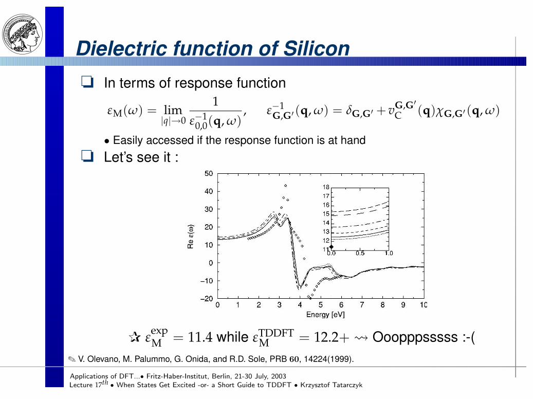
Dielectric function of Silicon

o In terms of response function

εM(ω) = lim|q|→0

1ε−1

0,0(q, ω), ε−1

G,G′ (q, ω) = δG,G′ + vG,G′

C (q)χG,G′ (q, ω)

• Easily accessed if the response function is at hand

o Let’s see it :

P εexpM = 11.4 while εTDDFT

M = 12.2+Ã Ooopppsssss :-(. V. Olevano, M. Palummo, G. Onida, and R.D. Sole, PRB 60, 14224(1999).


What is wrong ?

o The formulation strictly valid for localised systems onlyn we requested that the density & currents vanish at ∞

n RG theorem holds, provided that∮

n(r, t0)[∇u2(r)] · df ≡ 0

o The corespondence v(r, t) n(r, t) is proven by v(r, t) j(r, t)and then j(r, t) n(r, t)

o What happens if we choose the current density as a basicvariable ?

12

[

p +1c

Aeff[j](r, t)]2

+ veff(r, t)

φ(r, t) = i∂tφ(r, t)

j(r, t) = =∑iocc

φ∗i (r, t)∇φi(r, t) −

1c

n(r, t)Aeff(r, t)

o TD-Current-DFT Aeff = Aext + AH + AT + Axc

o Exc = iωc Axc = αPmac + ωβjT

. G. Vignale and W.Kohn, PRL, 77, 2037(1996). . N.T. Maitra, I. Souza, and K. Burke, to appear in PRB.


Dielectric function of Silicon...again

o Does it work now ?

P εexpM = 11.4 ≈ εALDA

M = 11.6. F. Koostra, P.L. de Boeij, and J.G. Snijders, J.Chem.Phys. 112, 6517(2000).



Summary

o Charge-neutral (optical) excitations can be convenientlyaccessed via time-generalisation of DFT

o The excitations can be studied through :

n time-evolution of a system under perturbation

n linear-response approach

o Due to early stage of development, the results usually are inqualitative/quantitative agreement with experiment

o Better description of XC effects desperately needed

o Many open questions await to be answered

Documents

When States Get Excited or a Short Guide to time ...th.fhi-berlin.mpg.de/th/Meetings/FHImd2003/Dtalks/FHI-WS...Lecture 17th † When States Get Excited -or- a Short Guide to TDDFT