simulating REALITY™

An Introductory Guide to Nonlinear Analysis

When f=Ku

sim

ula

ting

RE

ALI

TY

™

Nature is nonlinear. Although, for our own understanding, we often look to simplify the world around us, ultimately we need to come to terms with the fact that nature and hence engineering science is inherently nonlinear, either due to material or geometry effects or other multi-physics characteristics. With the increase of hardware capacity and software improvements in the last decade, the linearisation of real life engineering problems is no longer necessary, and more and more virtual simulations are being performed using nonlinear techniques. Automotive, aerospace, marine/naval, defense, construction, biomedical and packaging are just some of the industries where nonlinear techniques are used at this moment.

Virtual Product Development is already established as a standard component in nearly every commercial design to manufacture process. Widely accessible, infinitely variable, and highly cost effective, today’s computer aided technologies allow almost every aspect of design, performance, and manufacture, to be exhaustively explored by manipulation of potential design solutions in a virtual development environment.

This publication is intended as an introductory guide to some of the concepts of nonlinear simulation, and a description of some of the applications in engineering and manufacturing industry.

INDEX

1. INTRODUCTION 41.1 Structural Analysis Origins 41.2 Finite Element Analysis History 4

2. THE CHARACTERISTICS OF NONLINEARITY 52.1 Geometric Nonlinearity 52.2 Material Nonlinearity 52.3 Boundary Condition Nonlinearity 5

3. NONLINEAR FEA CONCEPTS 73.1 Small Strains 73.2 Nonlinear Strain-Displacement (Compatibility) Relationships 73.3 Nonlinear Stress-Strain (Constitutive) Relationships 73.4 Updated Equilibrium Confi guration 93.5 Incremental-Iterative Solution Procedure 9

4. LARGE DEFORMATIONS: MORE ABOUT GEOMETRIC NONLINEARITY 9 4.1 Total Lagrangian Description 114.2 Updated Lagrangian Description 114.3 Eulerian Description 11

5. PLASTICITY: MORE ABOUT MATERIAL NONLINEARITY 115.1 Time-Independent Behaviour 115.2 Time-Dependent Behaviour 115.3 Yield Criteria 135.4 Work Hardening 135.5 Creep 135.6 Visco-Elasticity & Visco-Plasticity 135.7 Rubbers & Elastomers 15

6. MORE ABOUT BOUNDARY CONDITION NONLINEARITY 156.1 Contact & Friction 15

7. NONLINEAR DYNAMIC ANALYSIS 167.1 Dynamic Solution Procedures 167.2 Implicit Methods 167.3 Explicit Methods 167.4 Implicit vs. Explicit 17

8. VIRTUAL MANUFACTURING 17

9. SOME PRACTICAL INFORMATION 179.1 Nonlinear Procedure 179.2 Mesh Refi nement & Rezoning 17

CASE STUDIES

Automotive Supply Nonlinear Simulation Aids Automotive Glass Development 6 Aerospace Sikorsky Aircraft Uses Nonlinear Solution to Reduce Design Bottlenecks 8 Manufacturing Process Invernizzi Presse Gain Precision and Safety with Nonlinear Simulation 10 Consumer Goods Simulation Helps LEGO Make Itt Right First Time 12 Construction Nonlinear Simulation of Infl atable Dam Enables Successful First Time Operation 14

3

(N). Hooke theorised a simple linear relationship between force applied and the associated defl ection, f = Ku. Thus, the defl ection (u) can be easily calculated by dividing the force applied by the stiffness coeffi cient. Today’s practical applications of such linear systems are somewhat more complex, and are solved by means of ‘matrix’ computational methods. The force and displacement quantities ‘become vectors‘. Potentially containing entries at all points in the structure, and the stiffness becomes a matrix of individual stiffness components assembled from each ‘element’ in the structure. However, the underlying principle is basically the same. Knowing the force (or in some cases the prescribed displacement) and the ‘stiffness’ of the structure, allows the associated ‘unknown’ to be calculated. Most analyses subsequently continue with downstream calculations to derive associated measures such as strain and stress, and then to use these for performance, design or other visualization purposes.

Such structural calculations are of course only valid where a linear relationship between force and displacement can be assumed to exist. That is, if one applies twice the force, the spring will defl ect twice as much. In reality all forms of structural mechanics exhibit nonlinear behaviour, whereby the stiffness of a structure progressively changes under increased loading, as a result of material changes, and/or geometric and contact effects. The end result is that the force applied and the displacement observed are no longer linearly proportional. The simulation of such behaviour characterises ‘nonlinear analysis’ and can be summarized by the equation f ≠ Ku. Both for mathematical and computational convenience early FE calculations assumed that a linear structural response was indeed a good approximation, especially for the relatively small

displacements (that is, relative to the structural dimensions themselves) and the materially elastic behaviour which were commonly considered in structures such as buildings and aircraft. However, as computational techniques have evolved, and computer hardware capacities expanded, it is now increasingly common for engineering designers to step closer to the physical reality of their designs, and to include nonlinear effects in their calculations. Indeed many designs, for example automotive crash structures, deformable packaging, locking & sealing systems, and many more, are completely reliant on nonlinear behaviour in order to function as intended. In these and many other cases the assumption of linearity is no longer an acceptable approximation. Nonlinear behaviour is also widely exploited in the simulation of the manufacturing process itself, with applications such as metal and plastics forming, pre-stressing, and heat treatment.

1.2 Finite Element Analysis History

In the mid-1950’s, American and British aero-nautical engineers developed the fi nite element method to analyse aircraft structures. Although the earliest calculations bore only a passing resemblance to FE method as we know it today, the underlying principles of discretisation (meshing), equilibrium (internal/external force balance), and constitutive modeling (materials) still formed the basis of the calculations.

Discretisation (more commonly known as ‘meshing’) refers to the way in which a complex structural component can be subdivided into a large, but fi nite number of relatively simple ‘elements’. By forming the stiffness characteristics of each individual element and combining those together into an inter-connected system of simultaneous equations, these engineers were

1. INTRODUCTION

Analysis in structural or mechanical engineering means the application of an acceptable analytical procedure based on engineering principles. Analysis is used to verify the structural, thermal, or other multi-physical integrity of a design. Sometimes, for simple structures, this can be done using handbook formulas or other closed form solutions. More often, however, this type of analysis relates to complex components or structural assemblies and is performed using computational simulation, part of the process of a Virtual Product Development (or VPD) approach.

The predominant type of engineering software used in these analyses is based on the Finite Element (FE) method, giving rise to the commonly used term Finite Element Analysis (FEA). Over the past 50 years, FEA has been successfully applied in all major industries, including: aerospace, automotive, energy, manufacturing, chemical, electronics, consumer, and medical industries. FEA is indeed one of the major breakthroughs of modern computational design engineering.

This guide is designed as an introduction to what is a complicated subject. It outlines some of the principles of nonlinear analysis, and describes some typical applications.

1.1 Structural Analysis Origins

The origins of structural mechanics go back to early scientists such as Isaac Newton and Robert Hooke. All physics students learn Hooke’s Law, as illustrated by a simple spring, with stiffness K (N/m), and loaded at the free end by a force F

4

able to extend Hooke’s basic principles into a robust and computationally efficient solution process. Although somewhat limited in complexity and restricted by the computational equipment of the time, these calculations formed the practical origins of today’s vast array of FE-based technologies.

In the 1960’s, researchers also began applying the finite element method to non-structural related fields in engineering science, such as fluid mechanics, heat transfer, electromagnetic wave propagation, and other field problems. In fact, many engineering a scientific computations can be solved based on similar principles, that is the solution of differential equations by setting up and solving systems of simultaneous equations. Theorists proved that in general, provided some mathematical conditions are met, the method converges to the correct theoretical results. Around this time, researchers also started applying FEA to nonlinear problems, looking at situations where linear assumptions were no longer vallid .

2. THE CHARACTERISTICS OF NONLINEARITY

As already described, all physical processes are to some degree nonlinear. For example, pressing an expanded balloon to create a dimple (the stiffness progressively increases, that is the rate of deflection decreases the more squeezing force is applied), or flexing a paper-clip until a permanent deformation is achieved (the material has undergone a permanent change in its

characteristic response). These cases and many other common everyday applications all exhibit either large deformations, and/or inelastic material behavior.

So where does nonlinear behaviour originate, and how can we assess its significance? In general there are three major, and most common, sources of nonlinear structural behaviour.

2.1 Geometric Nonlinearity

Structures whose stiffness is dependant on the displacement which they may undergo are termed geometrically nonlinear. Geometric nonlinearity accounts for phenomenen such as the stiffening of a loaded clamped plate, and buckling or ‘snap-through’ behaviour in slender structures or components. Geometric nonlinearity is often more difficult to characterize than purely material considerations. Geometric effects may be both sudden and unexpected, but without taking them into account any computational simulation may completely fail to predict the real structural behaviour.

2.2 Material Nonlinearity

Material Nonlinearity refers to the ability for a material to exhibit a nonlinear stress-strain (constitutive) response. Elasto-plastic, crushing, and cracking are good examples, but this can also include time-dependant effects such as visco-elasticity or visco-plasticity (creep). Material nonlinearity is often (but not always) characterised by a gradual weakening of the structural response as an increasing force is applied, due to some form of internal decomposition.

2.3 Boundary Condition Nonlinearity

Early FE analyses were typically performed on single structural components which underwent relatively small displacements. However, when considering either highly flexible components, or structural assemblies comprising multiple components, progressive displacement gives rise to the possibility of either self or component-to-component contact. This characterises to a specific class of geometrically nonlinear effects known collectively as boundary condition or ‘contact’ nonlinearity. In boundary condition nonlinearity the stiffness of the structure or assembly may change (considerably) when two or more parts either contact or separate from initial contact. Examples include bolted connections, toothed gears, and different forms of sealing or closing mechanisms.

Again, in reality many structures exhibit combinations of these three main sources of nonlinearity, and the algorithms which solve nonlinear equations are generally set up to handle nonlinear effects from a variety of sources.

To find evidence of possible nonlinear behavior, look for characteristics such as permanent deformations, and any gross changes in geometry. Cracks, necking, thinning, distortions in open section beams, buckling, stress values which exceed the elastic limits of the materials, evidence of local yielding, shear bands, and temperatures above 30% of the melting temperature are all indications that nonlinear effects may play a significant role in understanding the structural behaviour.

5www.mscsoftware.com

WHEN F≠KUAn Introductory Guide to Nonlinear Analysis

To predict the behaviour of the various materials, both in the different production stages and in their fi nal car-mounted position, Guardian Automotive use nonlinear simulation, with two main situations being considered. Firstly, to predict the temperature distribution over the entire window as the heating elements ar applied. This enables the identifi cation of hot spots, which may possibly cause weakness. Secondly, simulation of the manufacturing process in order to obtain the right shape for the window. Each car has its own characteristics, and each window must therefore be tailor-made. Windows are heated to obtain the right shape with various temperature situations being simulated in order to calculate how the bending process will develop. This is a complex nonlinear process taking into account the material construction, and the characteristics of the furnace and heating process itself. Simulation provides a repeatable and cost effective method for optimising the manufacturing process before production commences.

Guardian has worked with software from MSC.Software since 1983 and with MSC.Marc since 1998.

The decision to use MSC.Marc was based on its suitability for analysing the layout of the heating elements in rear windows. MSC.Marc was also used to simulate the glass bending process, providing vital information on the progress of various stages of the production. ”MSC.Marc is ideal for this; it was exactly what we were looking for. We were able to substitute numerical simulation for the physical development runs, which was very cost-effective”, Charles Courlander, Senior

AUTOMOTIVE SUPPLY

The manufacture of car windows requires a complex production process, as several variable factors are involved. Using nonlinear software tools from MSC.Software, Automotive manufacturer Guardian Automotive is developing simulation techniques to obtain an accurate prediction of how these factors will interact.

Employing 19,000 people around the world, Guardian is one of the largest global producers of fl at glass and the downstream automotive and architectural products made from this. The automotive products division has two European production plants, in Spain and in Luxembourg. These factories deliver directly to major car manufacturers as well as to car repair businesses. Both involve complex manufacturing processes, requiring a continuous operation environment.

One of the primary tasks is to optimize the production processes, on the one hand to enable Guardian to meet the wishes and demands of the car manufacturers, and on the other hand to generate the necessary internal effi ciency.

Nowadays all data relating to the production environment (for example attachment strips, rain detectors, mirrors, Aerial and heating elements) are stored in the CAD environment. For both single sheet and laminated glass the design factors include the requirements of sound insulation, security, visual distortion, and safety.

Nonlinear Simulation Enhances Production Process For Automotive Glass

Heating backliteHeating frontlite

6

CASE STUDY

Development Engineer, Gaurdian Automotive Luxembourg.

Nonlinear simulation has now become indispensable for Guardian. The automotive manufacturer presents the desired design layout for the window, including the position of the heating elements, mirrors, aerial and rain detector. All these factors are taken into account in the simulation allowing a rapid demonstration of the suitability or otherwise of any given confi guration.

Now that the current simulation methods have been developed effectively, Guardian is devoting time to the perfection of the methods. Implementation of a ‘gateway’ will facilitate the integration of the MSC.Software simulation software into Guardian’s existing CATIA design environment. This will allow for more effi cient meshing and geometry transfer, and will allow designers to work directly on the simulation models. ”With less time being spent on setting up the simulation environment, we can devote more time to our profession. We want to concern ourselves with the glass itself. Glass is our core business. Simulation is just a facilitator – but a very important one”.

3. NONLINEAR FEA CONCEPTS

For all FE analysis it is important to recognise that, whether linear or nonlinear, the FE method is an approximation to reality, the success of which is dependent on making good and overall balanced judgments on issues such as:

· The ‘quality’ of the FE model (geometric accuracy)· The discretisation process (choice, creation, and distribution of the mesh)· Material properties and related assumed behaviour· Representation of loadings and boundary conditions· The solution process itself (solution method, convergence criteria, etc.)

It is also important to recognise that, at least in principle, nonlinear applications are inherently more complex to execute than linear applications. For example the principle of ‘superposition’ (in which the resultant defl ection, stress, or strain in a system due to several forces is simply the algebraic sum of their effects when separately applied) no longer applies. Other linearising assumptions also require examination for their validity, such as the relationship between strain and displacement, that between stress and strain (the material or constitutive relationship), and the treatment of contacting bodies.

Although modern FE programs routinely include a signifi cant library of inherent intelligence, diagnostics, and self correction, the analyst‘s experience is still critical to the success or otherwise of a nonlinear analysis.

In nonlinear FEA, some or all of the following ‘linearising’ relationships may be violated:

3.1 Small Strains

Most metallic materials are no longer structurally useful when the strain exceeds one or two percent. However, some materials, notably rubbers, other elastomers, and plastics, can be strained to hundreds of a percent. Such applications require a redefi nition of traditional measures of ‘engineering’ (or small) strain.

3.2 Nonlinear Strain-Displacement (Compatibility) Relationhips

Applications involving large structural rotations (even for small strains) can violate traditional linear strain-displacement relationships. In such cases the changes in the deformed shape can no longer be ignored. The physics of buckling, rubber analysis, metal forming, and many other common applications, require that the often ignored higher derivative terms in the strain displacement relationship are incorporated into the formulation. Such analyses may use strain-displacement measures such as Green-strain or logarithmic strain. In these circumstances, traditional stress measures (often referred to as 2nd Piola-Kirchoff stress) are also invalid since the area over which the internal force is integrated in order to calculate the stress may have changed from the original undeformed confi guration. Consequently nonlinear strain-displacement relations are typically accompanied by the use of a Cauchy stress measure where the current state and position of the structure is always utilised in the stress calculation.

3.3 Nonlinear Stress-Strain (Constitutive) Relationships

Perhaps easiest to understand, nonlinear constitutive relationships relate to the progressive change in a material response according to the amount of strain (indirectly the displacement) which it experiences.

Plasticity is a very common example. Initially characterised by a near linear response, ‘plastic’ materials typically experience a yield ‘point’ after which their ability to carry increased load is signifi cantly reduced. If the material is unloaded the post-yield strain level produces a permament material deformation, or ‘set’. Under the continuation of loading, plasticity may continue develop until displacements effectively become infi nitely large for an infi nitely small increase in load. At this stage the material is assumed to be ‘fully’ plastic and has lost all structural engineering performance. Far from being a disadvantage, softening behaviour of this nature is specifi cally designed into the behaviour of many ‘designed to fail’ components such as safety enclosures in cars. Plastic fl ow is also central to manufacturing processes such as the forming or shaping of metals or other elasto-plastic materials.

In some cases post-yield hardening may occur as strains further increase. Plastic deformation also may exhibit sign (tension or compression), direction (fi bre reinforced plastics), time (visco/creep effects), or temperature (thermal) dependance, adding further to the complexity of the mathematical material description required. Metals, plastics, soils, rocks and many other materials exhibit different forms of elasto-plastic behaviour under a variety of different loading conditions. Many other

www.mscsoftware.com

WHEN F≠KU

7

An Introductory Guide to Nonlinear Analysis

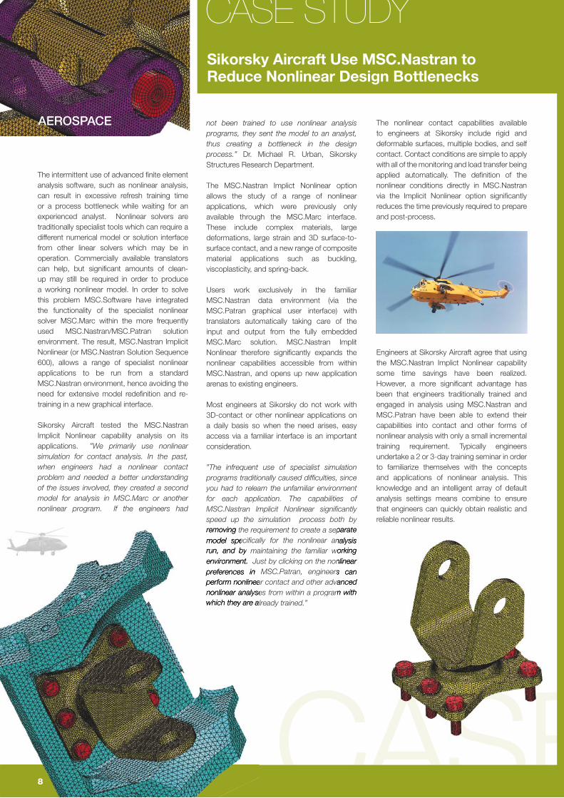
not been trained to use nonlinear analysis programs, they sent the model to an analyst, thus creating a bottleneck in the design process.” Dr. Michael R. Urban, Sikorsky Structures Research Department.

The MSC.Nastran Implict Nonlinear option allows the study of a range of nonlinear applications, which were previously only available through the MSC.Marc interface. These include complex materials, large deformations, large strain and 3D surface-to-surface contact, and a new range of composite material applications such as buckling, viscoplasticity, and spring-back.

Users work exclusively in the familiar MSC.Nastran data environment (via the MSC.Patran graphical user interface) with translators automatically taking care of the input and output from the fully embedded MSC.Marc solution. MSC.Nastran Implit Nonlinear therefore signifi cantly expands the nonlinear capabilities accessible from within MSC.Nastran, and opens up new application arenas to existing engineers.

Most engineers at Sikorsky do not work with 3D-contact or other nonlinear applications on a daily basis so when the need arises, easy access via a familiar interface is an important consideration.

”The infrequent use of specialist simulation programs traditionally caused diffi culties, since you had to relearn the unfamiliar environment for each application. The capabilities of MSC.Nastran Implicit Nonlinear signifi cantly speed up the simulation process both by removing the requirement to create a separate model specifi cally for the nonlinear analysis run, and by maintaining the familiar working environment. Just by clicking on the nonlinear preferences in MSC.Patran, engineers can perform nonlinear contact and other advanced nonlinear analyses from within a program with which they are already trained.”

The nonlinear contact capabilities available to engineers at Sikorsky include rigid and deformable surfaces, multiple bodies, and self contact. Contact conditions are simple to apply with all of the monitoring and load transfer being applied automatically. The defi nition of the nonlinear conditions directly in MSC.Nastran via the Implicit Nonlinear option signifi cantly reduces the time previously required to prepare and post-process.

Engineers at Sikorsky Aircraft agree that using the MSC.Nastran Implict Nonlinear capability some time savings have been realized. However, a more signifi cant advantage has been that engineers traditionally trained and engaged in analysis using MSC.Nastran and MSC.Patran have been able to extend their capabilities into contact and other forms of nonlinear analysis with only a small incremental training requirement. Typically engineers undertake a 2 or 3-day training seminar in order to familiarize themselves with the concepts and applications of nonlinear analysis. This knowledge and an intelligent array of default analysis settings means combine to ensure that engineers can quickly obtain realistic and reliable nonlinear results.

The intermittent use of advanced fi nite element analysis software, such as nonlinear analysis, can result in excessive refresh training time or a process bottleneck while waiting for an experienced analyst. Nonlinear solvers are traditionally specialist tools which can require a different numerical model or solution interface from other linear solvers which may be in operation. Commercially available translators can help, but signifi cant amounts of clean-up may still be required in order to produce a working nonlinear model. In order to solve this problem MSC.Software have integrated the functionality of the specialist nonlinear solver MSC.Marc within the more frequently used MSC.Nastran/MSC.Patran solution environment. The result, MSC.Nastran Implicit Nonlinear (or MSC.Nastran Solution Sequence 600), allows a range of specialist nonlinear applications to be run from a standard MSC.Nastran environment, hence avoiding the need for extensive model redefi nition and re-training in a new graphical interface. Sikorsky Aircraft tested the MSC.Nastran Implicit Nonlinear capability analysis on its applications. ”We primarily use nonlinear simulation for contact analysis. In the past, when engineers had a nonlinear contact problem and needed a better understanding of the issues involved, they created a second model for analysis in MSC.Marc or another nonlinear program. If the engineers had

Sikorsky Aircraft Use MSC.Nastran to Reduce Nonlinear Design Bottlenecks

removing the requirement to create a separate model specifi cally for the nonlinear analysis run, and by maintaining the familiar working environment. Just by clicking on the nonlinear preferences in MSC.Patran, engineers can perform nonlinear contact and other advanced nonlinear analyses from within a program with

removing the requirement to create a separate model specifi cally for the nonlinear analysis run, and by maintaining the familiar working environment. Just by clicking on the nonlinear preferences in MSC.Patran, engineers can perform nonlinear contact and other advanced nonlinear analyses from within a program with which they are already trained.”

AEROSPACE

8

CASE STUDY

forms of material nonlinearity also exist, of which cracking/fracture, crushing (concretes/foams), and de-lamination (laminated composites) are perhaps the most commonly encountered.

3.4 Updated Equilibrium Confi guration

Equilibrium is one of the under-pinning principles of the FE method, and ensures that externally applied forces and internally generated states of stress are balanced. The overall result of nonlinearity (from whatever source of origin) is that the force-displacement relationship requires continual updating in order to maintain equilibrium, and hence the physical validity of the simulation. As we will see, numerical equlibrium is typically maintained by solving nonlinear applications with an ‘incremental-iterative’ approach.

3.5 Incremental-Iterative Solution Procedures

As already discussed, FEA is an approximate technique. The method of solution of the simultaneous equations which describe the physics of any application is one of the important consideration, especially when the application is nonlinear in nature.

In a simple linear analysis, the load are applied and the displacements are calculated from a relatively simple inversion of the stiffness matrix. In theory the ‘value’ of the load is unimportant since the linearity of the response and the principle of superposition can be used to extrapolate to any desired loading magnitude.

In nonlinear analysis the non-proportionality between the applied load and the resulting displacements (the result of the inherent

nonlinearity in the structural stiffness) is accounted for by applying the load in a series of steps or ‘increments’. Early nonlinear analyses used a purely incremental approach, but depending on the size of the increments used and the degree of nonlinearity encountered such techniques often diverged from the true structural behaviour. In today’s solutions, within each load increment the loss of equilibrium between individual load increments is corrected using an iterative technique. The details of this process are unimportant here, suffi ce that the subsequent recalculation of internal stresses progresses until the equilibrium balance is restored (in practice a small out of balance is normally tolerated subject to some ‘convergence criteria‘). Such methods are therefore referred to as ‘incremental-iterative’ (or Newton-Raphson) methods and widely used in nonlinear analysis.

The construction and inversion of the stiffness matrix is one of the major computational overheads in performing a nonlinear analysis. This is especially true for models with a large number of degrees of freedom, and/or a large number of loading increments. In the standard Newton-Raphson method the stiffness matrix is reformed at each iteration of each increment in the process. The continually current nature of the structural stiffness means that using standard Newton-Raphson methods convergence is usually fairly rapid (few correcting iterations are required). However, the computational expense of each iteration can be considerable. For this reason ‘modifi ed’ Newton-Raphson methods are often used, in which the stiffness matrix is reformed less frequently (perhaps just on the fi rst or second iteration of each increment where the stiffness changes most signifi cantly). Modifi ed

Newton-Raphson methods as described above generally converge less rapidly (more iterations are required) but a net gain in computational effi ciency is achieved in the less frequent formation and inversion of the stiffness matrix.

The computational aspects of nonlinear equation solution have been subject to a great deal of research, and in most of today’s nonlinear FE codes you will fi nd a number of variations or alternative solution procedures such as:

· Strain Correction Methods· Secant or Conjugate-Gradient Methods· Direct Substitution Methods· Quasi-Newton Methods

4. LARGE DEFORMATIONS: MORE ABOUT GEOMETRIC NONLINEARITY

In implicit nonlinear analysis, using the Newton- Raphson procedure, the relationship between the incremental load and the associated displacement is called the tangent stiffness KT. In general this stiffness is comprised of three components: · Material stiffness · Initial stress stiffness· Geometric stiffness

The material stiffness may be the same elastic stiffness as used in linear FE solutions. The initial stress stiffness term represents the resistance to load caused by realigning the current internal stresses when displacements occur. The fi nal component, the geometric stiffness, represents the additional stiffness due to any nonlinearity in the strain-displacement relationship.

9www.mscsoftware.com

WHEN F≠KUAn Introductory Guide to Nonlinear Analysis

and connecting rods is used to evaluate the bending stresses in the pivot, the contact pressure on the bearing, and the resulting rod stiffness. The thermo-mechanical properties of the bearing is also considered since the heat generated by the friction between the parts increases the temperature of the mechanical components, and can break the oil fi lm causing seizure of the mechanism. Mechanical safety is also monitored with MSC.Marc allowing engineers to study the mechanical behaviour of the safety system used on all types of presses. The analysis uses fl exible contact elements and an external force representing the oil pressure. Finally, Epicycloidal analysis (study of a multi-stage gear transmission system) allows engineers to evaluate the stresses in complex gear systems in order to optimise the gear dimensions, avoid gear failure during duty cycles, and extend the life of the mechanism.

Using the results of these simulations, Invernizzi can demonstrate the functional performance of a press without having to build a physical prototype, illustrating to its customers that the press will fulfi l the requested tasks. This is especially important when a custom-made press is needed, since the production of a physical prototype would be impossible due to cost and time restraints. In addition to a virtual demonstration of how the press will work, suggestions for custom-made presses can be based on the analysis results provided by MSC.Marc and MSC.Patran.

Before using MSC.Marc, the development department of Invernizzi Presse used department of Invernizzi Presse used mathematical methods to complete the mathematical methods to complete the calculations for the presses. These methods calculations for the presses. These methods were time-consuming and less precise be-were time-consuming and less precise be-

cause only a certain number of design variations could be tested. Using MSC.Marc it is easy to change the geometry of the coupling and the material characteristics for each type of press, or to optimise the weight of any design confi guration. Different analyses with different materials can be performed easily and help to choose the best type of material in less time. MSC.Marc is also used to analyse critical safety issues associated with high operating temperatures of the working presses.

Luigi Piccamiglio is convinced that Invernizzi will continue using MSC.Marc and MSC.Patran, and will look to extend their capability by including other MSC.Software products into their process. ”MSC.Marc gives us confi dence in our results and offers a complete list of features. I am very satisfi ed with the results of our analyses, and our collaboration with MSC.Software has been a fruitful one. We are also interested in dynamic simulation with MSC.ADAMS in order to study and optimize the link-drive mechanisms. I expect the integration of MSC.ADAMS and MSC.Marc will bring many advantages to our development process.”

With more than 40 years experience in the construction and development of mechanical presses, Invernizzi Presse from Pescate LC in Italy produces some of the safest and most technologically advanced metal forming presses offered on the market today. In addition to their standard mechanical presses, Invernizzi Presse offers custom-made presses, designed and built to meet the needs of individual customers. Invernizzi’s broad product portfolio, high-quality materials, and technological expertise meet the industry’s stringent requirements for safety, robustness, functionality, versatility, and durability.

When introducing simulation to their product development process Invernizzi Presse performed a benchmark of different fi nite element method software packages to fi nd the best analysis tool.

”I studied the principal providers of nonlinear FEA software, and decided on MSC.Marc because it is the best solution for our application. We needed to study an assembly of parts that are in contact with one another. MSC.Marc is a very good product to study both contact and the thermo-mechanical behavior of contacting parts”. Luigi Piccamiglio, Research & Development Engineer, Invernizzi Presse.

Invernizzi Presse use the combination of MSC.Marc and MSC.Patran in a variety of applications in their forming process. Contact analysis between pivot, bearing,

Invernizzi Presse Gain Precision and Safety with Nonlinear Simulation

of applications in their forming process. Contact analysis between pivot, bearing,

MANUFACTURINGPROCESS

10

CASE STUDY

physical prototype would be impossible due to cost and time restraints. In addition to a virtual demonstration of how the press will work, suggestions for custom-made presses can be based on the analysis results provided by

Before using MSC.Marc, the development department of Invernizzi Presse used mathematical methods to complete the calculations for the presses. These methods were time-consuming and less precise be-

As previously described, in solving this type of problem the load is increased in small increments and the incremental displacement is found using the current (or near current) approximation to the tangent stiffness. However, in geometrically nonlinear (or large displacement) analyses there are a number of different ways in which the geometric state of the structure can be described. Understanding these descriptions is important as they have implications for interpreting the results of the analysis performed.

4.1 Total Lagrangian Description

In a ‘Total Lagrangian’ method all calculations, at each stage of the incremental loading history, are always referred to the original (undeformed) geometry. For example the calculation of items such as stress always utilise the original representative ’area’ in the force/area calculation. Total Lagrangian methods are therefore generally suitable for applications which exhibit large displacements and large rotations, but where strains are generally small.

4.2 Updated Lagrangian Description

As the name suggests, an ‘Updated Lagrangian’ method always uses the current (deformed) confi guration of the structure for calculation. This requires the FE mesh coordinates to be updated at each increment in order to form a new ‘reference geometry’. For this reason an Updated Lagrangian approach is more suitable to applications such as metal forining, which exhibit large inelastic strains.

4.3 Eulerian Description

A Eulerian description has a major difference in approach. In a Eulerian method it is assumed that as the material of the structure deforms its

motion is described relative to a fi xed spatial geometry, that is the material fl ows through a fi xed frame of geometric reference. This approach has major advantages when describing materials which essentially fl ow, such as structural forming, extrusion or classical fl uid dynamics.

In some cases it is highly convenient to mix these formulations. For example in MSC.Dytran the structure-fl uid coupling, is achieved by combining a Lagrangian type formulation for the structural aspects of the model, with a Eulerian approach to describe the motion of the fl uid components. Such descriptions are of course purely mathematical conveniences, but are highly useful for coupled applications such as the sloshing of fuel tanks, the gas dynamics of airbags in passenger safety, aero-engine bird strike, helicopter sea-ditching and many more.

5. PLASTICITY: MORE ABOUT MATERIAL NONLINEARITY

In reality all materials, even when subjected to relatively small loadings exhibit some degree of nonlinear behaviour. However, for the purposes of FE analysis it is convenient to idealise many everyday engineering materials as generally having an elastic initial response (that is, a proportionality of strain and stress, and a return to a initial state should a load be removed), and an inelastic (often plastic) response once some threshold of stress has been achieved. Plastically deformed materials exhibit different stiffness characteristics to their original elastic state and show permanent deformations if the loading is removed. As we will see, there are a large number of theoretical material models which attempt to describe both simple and complex elasto-plastic behaviour.

However, before we look at these material models in more detail, it should also be noted that when stresses increase beyond the linear elastic range, material behavior can be broadly divided into two classes:

· Time-Independent Behaviour· Time-Dependent Behaviour

5.1 Time-Independent Behaviour

In this case there is no subsequent straining should loadings be maintained over a long period of time. This applies to many ductile metals, and in the case of nonlinear elasticity to rubbers and other elastomers. Conversely strains are not assumed to be affected should very short term loadings be applied, for example in the case of highly dynamic loading conditions such as explosions.

5.2 Time-Dependent Behaviour

Often referred to as ‘visco’ effects (visco-elasticity, or visco-plasticity) or more simply ‘creep’, time-dependent materials are assumed to develop additional straining over long periods of time, or to demonstrate strain-rate effects typically under very short term but usually high intensity loadings. Elevated temperature conditions also contribute to time-dependent effects. Visco-plasticity is typically applicable to high-temperature applications. Visco-elasticity is used for elastomers, glass, and plastics.

Plasticity (material nonlinearity as a whole) is a huge science and the subject of a wealth of reference material. Here we hope to give an overview of the basics and a brief description of some of the more commonly used elasto-plastic material models.

11www.mscsoftware.com

WHEN F≠KUAn Introductory Guide to Nonlinear Analysis

cycle time, increase functionality of toys and make material/structural knowledge available to more people within the organization. By determining how a part will behave at an earlier stage, there are fewer changes made to tooling, so the costs associated with making a physical prototype and making changes to molds can be substantially cut.

FEM was implemented as a three-phase process, including proof of concept, training and production implementation. During the fi rst phase, LEGO benchmarked different FEM products, deciding on MSC.Marc, MSC.Patran and MSC.Nastran because of their features, ease of use and technical support. The second phase included training, and comparing simulation tests with known results to better understand how the software should be utilized. And the third phase, included implementing structural calculations in the development phase and establishing a FEM team that is capable of avoiding structural problems in LEGO tools and parts.

Testing conducted at LEGO Company specifi cally for safety includes compression, torque, tensile, drop and drop tests, as well as tests for sharp points and edges. Examples of these tests include linear stress analysis on a tool part for the 2x4 LEGO brick, using MSC.Nastran, and MSC.Marc, contact analysis on the same part to defi ne a more realistic boundary condition. Additionally MSC.Marc non-linear analysis is utilized to simulate a

compression test on the 1x16 LEGO TECHNIC element. On this same part, MSC.Marc can simulate a torque test or generate a force-displacement diagram for contact analysis.

One of many benefi ts LEGO Company has realized with FEM is improved design. “We’re not afraid to try a new solution. With simulation our designs have been more stable. Simulation provides an opportunity to try more solutions and have the confi dence that when you have a very strict schedule, and you come up with a virtual solution that it will work when it is made.”

With simulation, LEGO Company has reduced the overall cycle time, from concept to fi nished part. Another tangible benefi t of simulation is understanding where the stresses are and where they are not. With this knowledge an engineer can make what might seem to be a very insignifi cant change of mass. But the resulting material savings can be great, especially for high volume parts.

At the end of its two-year simulation implementation program, LEGO Company is quickly achieving its goals ensuring that safety and quality are the focus of new product development. At the same time, LEGO Company has reduced dependency on physical prototyping, eliminating costly changes to tooling, as well as substantially reduced manufacturing costs, including material and service life of molds.

Since 1932, the LEGO Company has been making its reputation for delivering quality products and experiences that stimulate creativity in children around the world. More than 1.4 million LEGO parts are produced every hour making up the 100 million LEGO sets produced annually. With this many parts, every part and every change, even small changes in material usage, have a tremendous impact on costs. To validate products before they go into production, maximizing safety, minimizing time-to-market and costs, the LEGO product development team uses MSC.Marc, MSC.Patran and MSC.Nastran simulation software. Over 300 engineers and managers develop new designs for the approximately 200 to 300 new parts designed each year. When you’re the leading manufacturer of products to stimulate creativity, imagination, fun and learning, you have everybody’s attention: customers and competitors. So maintaining state-of-the-art product development tools is imperative.

“The type of analyses that we do on plastic parts includes strength/stiffness, strength/thickness and fatigue analysis. Of course, the goal is to ensure safety, especially for products for the zero to fi ve year-old market, as well as reduce material usage where possible or change from one material to another. In the future, we will be coupling fl ow and structural analysis to get the ansiotropic material data and residual stresses that form the fi lling.” Mr. Jesper Kjærsgaard Christensen, LEGO Company CAE Consultant.

The FEM team at LEGO Company is responsible for virtual development of parts and tooling, beginning in the conceptual development phase. The objective is to focus on product safety, as well as reduce overall

Simulation Helps LEGO Make It Right First Time

CONSUMER GOODS

12

CASE STUDY

An elasto-plastic material may be defi ned as a material, which, upon reaching a certain stress state, undergoes continued deformation which is generally irreversible, resulting in behavior which is path-dependent. A basic assumption in elastic-plastic analysis is that deformation can be divided into an elastic part and an inelastic (plastic) part.

5.3 Yield Criteria

The yield stress is a measured stress value that marks the onset of lastic deformation. Its magnitude is usually obtained from a uniaxial test. However, since stresses in a structure are multi-axial, this uniaxial value is typically used in a multi-axial measure of yielding called the ‘yield condition’ or ‘yield criterion’.

The most widely used yield condition is the von Mises criterion in which yielding is assumed to occur when the level of effective stress (often referred to as ‘equivalent’ or von ‘Mises stress’) reaches the yield value as defi ned from a uni-axial test. This yield condition agrees fairly well with the observed behavior of many ductile metals such as low carbon steels and aluminum, and is widely used in materially nonlinear FE analysis.

Another commonly used yield condition is the Tresca condition, in which yielding occurs when the maximum shear stress reaches the value it has when yielding occurs in the tensile test.

Others such as the Drucker-Prager (or Mohr-Coulomb) methods, describe a yield surface which includes a dependence on an existing hydrostatic (or confi ning) state of stress. Mohr-Coulomb and Drucker-Prager models are often used to describe granular materials such as soils, rocks, ice, and concrete where confi ning or pre-stressing effects play an important part in the material behavior.

There are many more yield criteria such as modifi ed von Mises, Hill, Hoffman, Shima, and Gurson, accounting for the behaviour of a huge variety of materials, from clays, crushable foams, to fi bre-reinforced plastics. Many include different yield criteria for tensile, compressive, or mixed states of stress, or for materials which exhibit orthotropic or anisotropic properties. Other materials can be described by ‘progressive damage’ models in which the material degradation under increased stress is dealt with in a slightly different manner.

5.4 Work Hardening

In a uniaxial test, the work hardening slope (the post-yielding stiffness) is defi ned as the slope of the stress to plastic strain curve. It relates the incremental stress produced to the incremental plastic strain applied and dictates the conditions of post-yield material behaviour.

An ‘isotropic’ hardening rule assumes that the center of the yield surface remains stationary in the stress space, but the size (radius) of the yield surface expands due to strain hardening. This relates to generally non-dilatent materials and is considered suitable for problems in which the plastic straining far exceeds the incipient yield state. It is therefore widely used for simulations of the manufacturing processes and large-motion dynamic problems.

The ‘kinematic’ hardening rule assumes that the von Mises yield surface does not change in size or shape, but the center of the yield surface shifts in stress space. Straining in one direction reduces the yield stress in the opposite direction. It is therefore used in cases where it is important to model behaviour such as the Bauschinger effect.

5.5. Creep

Creep is continued deformation under constant load, and is a type of time-dependent inelastic behavior, which can occur at any stress level. It is an especially important consideration for elevated temperature stress analysis (e.g., in nuclear reactors) and in materials such as concrete. Creep behavior can be characterized in three stages: primary, secondary, and tertiary, and is generally represented by a Maxwell model, which consists of a series arrangement of a spring and a viscous dashpot.

For materials that undergo creep, with the passing of time the load decreases for a constant deformation. This phenomenon is termed ‘relaxation’.

5.6 Visco-Elasticity & Visco-Plasticity

Viscoelasticity, as its name implies, is a generali-sation of elasticity and viscosity. It is often represented by a Kelvin model, which assumes a spring and dashpot in parallel. Examples of visco-elastic materials are glass and plastics.

A viscoplastic material exhibits the effects of both creep and plasticity, and can be represented by a creep (Maxwell) model modifi ed to include a plastic element. Such a material behaves like a viscous fl uid when it is in the plastic state.

13

WHEN F≠KUAn Introductory Guide to Nonlinear Analysis

An FEA simulation using MSC.Marc was performed to calculate the effect of static stresses on the nonlinear material characteristics of the membrane, as well as understand performance of the infl atable dam and the infl ation/defl ation procedure. Scale models in the hydraulics lab were utilized for correlation with the FEA analysis and for investigating dynamic effects. Input for the analysis included environmental factors, such as temperature and pressure and the material properties of the fabric resulting from test coupons. The fabric for the membrane was made of rubber reinforced with nylon cord that is 16 mm thick, weighing 20 kilos per square meter. The membrane for one of the dams weighs in at 33 metric tons. The kinematic and constitutive equations of nonlinear material performance, as measured, are based on small strains, the so-called engineering values. In the MSC.Marc analysis the strains are measured in the large strain formulation, therefore to be able to apply the material data in the correct way, strains and stresses had to be converted between both formulations. This particular analysis was diffi cult since the membrane is built from a composite of rubber and nylon cord and is quite thin in comparison to its size, resulting in huge displacements which cause instability in the model. However, by applying consistent and very high tensile force to stretch the membrane it was possible to keep the model stable. As the stresses and loads were applied for the analysis, then the boundary conditions that kept the model stable were relieved.

The edges of the membrane are clamped to a sill at the bottom of the river so it is like a defl ated balloon lying on the bottom of the river. However, stresses were higher than acceptable at the clamping points in the fi rst analysis. By clamping the membrane away from the boundary, peak stresses reduced as the clamping forces were redistributed. Factors related to the excessive clamping stress were identifi ed in the fi rst analysis, enabling recommendations for improving the clamp design. MSC.Software worked together with the client to modify the design in such a way the stresses would be reasonable. The simulation determined a redesign with a sprung clamp and established the force required to start moving the membrane without inducing high stresses.

In October 2002, the sixth worst storm to hit the Netherlands since 1970 caused the infl atable dam to automatically deploy. Within an hour, the waters receded and the dam defl ated within one-hour’s time. ”The simulation performed by MSC.Software Professional Services using MSC.Marc has given us a good feeling for the behavior of the Ramspol rubber dam and has improved our knowledge of this kind of fl exible structures”.

Protecting the northwestern province of Overijssel in the Netherlands from fl ooding are three infl atable storm surge barriers designed by Hollandsche Beton-en Waterbouw bv (HBW), a design/build engineering fi rm head-quartered in the Netherlands. Because an infl atable dam of this size had never been built before, the concept had to be validated before it could be built. MSC.Software Professional Services was engaged to investigate the concept, as well as to make design improvement recommendations, using MSC.Marc nonlinear simulation software.

”A prototype, is typically a pass/fail situation, it either works or it doesn’t. Simulation of the infl atable dam provided the information that allowed us to understand its performance and ensure stresses were within the specifi ed margin of safety. With the infl atable dam, there was no alternative to simulation for validating the design.” Mr. Hans Dries, Project Manager, HBW.

The infl atable dams are 75m long, 13m wide, 8.35m high and made of rubber sheet reinforced with nylon cord. Automatically deployed by opening pipelines connecting upstream water with the interior of the infl atable dam, compressors located at each of its two ends simultaneously infl ate the membrane with air. The top of the infl atable dam is kept above the upstream water level normal with an internal air pressure, and as the water level rises, deformation of the membrane increases. The dams are defl ated by opening the air valves and pumping the water out.

Nonlinear Simulation Ensures First-Time Success of Infl atable Dam

CONSTRUCTION

CASE STUDY

14

5.7 Rubbers & Elastomers

An elastomer is a natural or synthetic polymeric material with rubber-like properties of high extensibility and fl exibility. Elastomers show nonlinear elastic stress-strain behavior, which means that upon unloading the stress-strain curve is retraced and there is no permanent deformation.

Rubber and elastomers also exhibit near incompressibility, showing almost zero volumetric change under load and a Poisson‘s ratio of approximately 0.5. This incompressibility constraint means that FEA codes can model these types of materials only if they have special element formulations (for example, ‘Herrmann elements’ or ‘mixed/hybrid formulations’) which are able to describe this type of extreme behaviour.

FEA codes with nonlinear elastic capability generally offer one or more hyper-elastic material models (strain energy functions), such as the two-constant Mooney-Rivlin model, one-constant Neo-Hookean model, and the fi ve-constant, third-order James-Green-Simpson model. The material constants used in these models are obtained from experimental data.

6. CONTACT: MORE ABOUT BOUNDARY CONDITION NONLINEARITY

Since the detection of contact (or separation) is dependent on a continual monitoring of an updated geometry confi guration, contact is by nature a type of geometric nonlinearity. However it is often referred to as boundary condition nonlinearity since the change in contact conditions act in a similar way to changes in boundary conditions such as loads or constraints.

During contact, mechanical loads, and perhaps thermal or other physical entities, are transmitted across the area of contact. If friction is present, shear forces are also transmitted.Contact can be modeled numerically in various ways. Early contact analysis required potential areas of contact to be pre-determined and connected by contact (or spring, or interface) elements. These elements exerted a contacting force once the separation of the contacting bodies was no longer evident. Although basically functional, such systems suffered the disadvantages of having to pre-defi ne and pre-connect potential areas of contact, and to assume a contacting stiffness through which to transfer loads. In practice this excludes all but the simplest of practical contact applications. Pre-defi ned contact in this manner was also unable to accurately model frictional or large relative sliding motions, and usually required a geometric simplifi cation of the contacting surfaces.

Consequently, most modern FE systems now use various forms of ‘slideline’ technology to model contact. For example, in MSC.Marc, areas of potential contact do neither need to be known nor specifi ed prior to the analysis. Potentially contacting surfaces are continually monitored, and the contact and separation conditions are automatically applied, transferring load (or other entities) accordingly.

Both deformable-to-rigid and deformable-to-deformable contact situations are generally allowed. Self-contact, such as is common in large deformation rubber problems, is also a comment requirement. The bodies can be either rigid or deformable, and the algorithm tracks variable contact conditions automatically. Rigid surfaces may be directly imported from a CAD system, and their exact mathematical form is used in the calculations. For a deformable body, the most modern techniques improve upon contact conditions monitored only at the edges of the

element by fi tting a curve or surface through the contacting boundary. This improves the accuracy of the solution by representing the geometry more faithfully than with discrete fi nite elements and is important for applications such as concentric shafts or rolling simulation. It also improves the typical slide/stick problems of curved contacting boundaries. The location and open/close status is handled automatically and there is no need to predetermine the ‘master’ and ‘slave’ components of early slideline technology. In coupled thermo-mechanical problems the contact or proximity of contact is also used to address convective, radiative and conductive heat transfer.

6.1 Contact & Friction

Two classical friction models are typically used: Coulomb friction and Shear friction. In addition, if necessary, user defi ned subroutines can be used to constantly monitor the interface conditions and modify the friction effect. In this way, friction can be made to vary arbitrarily as a function of location, pressure, temperature, amount of sliding, and other associated variables. In order to reduce numerical instabilities in the transition between sticking and slipping, a regularisation procedure is applied. Sometimes, the physics of deformation dictates modeling the regions of sticking fairly accurately (for example, driver pulley transferring torque through the belt to a driven pulley). For such cases, a stick-slip friction model based on Coulomb is also used.

Because friction generates heat, a coupled thermo-mechanical analysis is often required, especially in high friction rubber analyses such as rolling tyres. Frictional contact is used to model the behavior at the tyre footprint using Coulomb and shear friction models. The road surface and rim can also be represented as either rigid, or discretised into a deformable FEA mesh.

15www.mscsoftware.com

WHEN F≠KUAn Introductory Guide to Nonlinear Analysis

7. NONLINEAR DYNAMIC ANALYSIS

Incremental nonlinear FE solutions are often termed ‘quasi-static’. Although the loading is typically applied progressively in a number of increments, this process is purely a numerical convenience and does not represent the structural response over passing time. Even where creep or contact conditions are included, strictly speaking the nonlinear model is assumed to be ‘static’ (or at least quasi-static) in nature. In essence the structural mass is non-excitable (other than by gravity) and velocity and other acceleration effects are ignored.

Structural behaviour in which time effects are significant are referred to as ‘dynamic’ or ‘transient’. Again, for numerical purposes it is convenient to sub-classify dynamic FE applications into ‘modal’ or ‘frequency based’ problems, and those which are truly transient. Modal type applications use the frequency response of the structure to model effects such as natural and forced vibration. Although dynamic over given period these calculations can be simplified due to the ‘steady-state’ nature of their dynamic behaviour.

Truly transient effects are dealt with using a dynamic ‘step-by-step’ procedure in which the FE solution is progressed in a series of time steps. Dynamic FE simulations may of course be structurally linear, in terms of geometry, material response, or contact/boundary conditions. However where both transient and nonlinear effects are significant the FE solution performed is termed ‘nonlinear-dynamic’. Again, although in reality all applications are both nonlinear and dynamic in nature, the analyst may

look to make linearising or static assumptions about the behaviour in order to avoid such numerical complexity. Nonetheless, with improved FE technology, and faster and higher capacity computational systems, nonlinear dynamics analysis now makes up a significant proportion of the FE simulations performed. Automotive crash or other impact applications are good examples of where both nonlinear and dynamic effects are highly significant.

7.1 Dynamic Solution Procedures

In some respects, the solution of transient dynamics problems is a simple extension of standard linear or nonlinear static problems. The basic stiffness equations are augmented with velocity, damping, acceleration, and mass terms. In addition to a spatial or geometric discretisation, the time over which the dynamic effects take place is also ‘discretised’ into a number of time increments. The FE solution is then progressed through time in a step-by-step manner (hence the common reference to ‘step-by-step dynamics’) taking into account the velocity and acceleration response in addition to its pure force-displacement behaviour.

Most nonlinear dynamics FE codes offer one or both of two major approaches to dynamic equation solution, namely ‘implict’ and ‘explicit’ methods.

7.2 Implicit Dynamics Methods

An ‘implicit’ approach solves a matrix system, one or more times per step, in order to advance the solution. It is particularly appealing for a linear

transient problem, since it allows a relatively large time step to be applied – implicit methods can be shown to be numerically stable for large time steps, although it should be remembered that selection of a large time step may fail to capture some of higher frequency (or shorter time duration) components of dynamic structural behaviour. In implicit nonlinear analysis nonlinearities must occur within a time step, and this along with the frequent solution of potentially large systems of equations adds complexity and computational expense to implicit methods.

Examples of implicit approaches (or time-integration schemes) include: Newmark-beta (the most popular), Wilson-theta, Hilber-Hughes-Taylor, and Houbolt. Each has its own specific advantages and associated applications. Although generally highly stable some of these schemes have still been shown by researchers to exhibit numerical damping problems, sensitivity to time step size, or other stability problems, and the user should be aware of these when selecting a particular method.

7.3 Explicit Dynamics Methods

By contrast, an explicit approach advances the FE solution without (or at least less frequently) forming a stiffness matrix, a fact that makes the coding and the execution much more simple. For a given time step size, an explicit formulation generally requires fewer and less complicated computations per time step than an implicit one. Complicated boundary conditions or other forms of nonlinearity are also handled easily since nonlinearities are handled after a step has been taken. However explicit dynamics solution

16

methods are inherently unstable and rapidly diverge from a meaningful solution unless the time step applied is both relatively small and shorter than a calculated critical maximum value. This means that explicit analyses are generally charaterised by large number of relatively small time steps. This makes them much more suitable to short duration or highly dynamic applications such as explosive loading, or those where the material effects themselves are time dependent (strain-rate dependency). The most common explicit schemes use the ‘central-difference’ approach and should always be performed in conjunction with a time stepping algorithm which keeps below the critical stability limit.

7.4 Implicit vs. Explicit

The choice of whether to use implicit or explicit time integration schemes is an important consideration and depends on a number of factors including:

· Nature of the dynamic problem· Type of finite elements used in the model· Size of the model· Dynamic behaviour (notably the velocities of the problem compared to the speed of sound in the material).

8. VIRTUAL MANUFACTURING

Virtual Manufacturing involves the use of computational modeling to simulate not only a finished product but also the processes involved in its creation or fabrication. Such technology enables companies to optimise key manufacturing

factors which directly affect the profitability of their manufactured products. In addition to the overall product performance these factors include final shape, manufacturability, residual stress levels, and in service issues such as durability and robustness. Profitability is improved by reducing the cost of production, material usage, and warranty liabilities.

Nonlinear (and often nonlinear-dynamic) FEA technology lies at the core of Virtual Manufacturing, allowing companies to simulate fabrication and testing in a more realistic manner than ever before. Virtual Manufacturing reduces the cost of tooling, and reduces the need for multiple physical prototypes. The inherent repeatability of numerical modeling enables a ‘right the first time’ manufacturing environment, providing manufacturers with the confidence of knowing that they can deliver quality products to market on time and within budget.

From a business perspective, it is clear. Small improvements in manufacturing can have dramatic effects in terms of cost and quality. Return on Investment calculations show that small savings in material usage deliver potentially large returns in a manufacturing environment.

To summarize, some of the advantages of a Virtual Manufacturing process include:

· Improved performance and quality of product· Verification of designs before prototyping· Elimination of costly manufacturing iterations· Reduced material waste· Reduced time-to-market· Competitive advantage over Competitors

9. SOME PRACTICAL INFORMATION

9.1 Nonlinear Procedure

It is generally advisable to prepare for a nonlinear analysis by starting with a relatively simple model. Nonlinear behaviour can be complex to interpret so the gradual addition of new sources of nonlinearity into the model can help considerably with the understanding of the results obtained.

Whilst the final analysis should be executed with a refined mesh suitable to capture the nonlinearities involved, sample analyses involving coarser meshes will also help to keep the investigative trial models to a practical size and execution time.

9.2 Mesh Refinement & Rezoning

Due to potentially large relative deformations and the capture of nonlinear material effects it is common for nonlinear FE simulations to require more refined finite element meshes than for linear analysis. Finite elements are also known to lose accuracy when the original mesh becomes highly distorted. Modern FE codes account for this by providing facilities (either manual or automatic) to reconstruct or to rezone the mesh as the nonlinear solution progresses. The ability to improve the element shapes throughout the analysis is critical in large deformation applications such as metal forming.

17www.mscsoftware.com

WHEN F≠KUAn Introductory Guide to Nonlinear Analysis

www.mscsoftware.com

WHEN F≠KU

18 www.mscsoftware.com

This guide references a number of individual software products and services from MSC.Software. A brief description of the SimOffice, SimDesigner, and MSC.SimManager product lines is included for your information below. For further details please visit www.mscsoftware.com/products.

SimOffice™ is the stand-alone VPD environment for building, testing, reviewing, and improving integrated virtual prototypes. MSC.Software products including MSC.Nastran, MSC.Marc, MSC.ADAMS, MSC.Dytran, MSC.Patran and others, all form part of SimOffice and are accessible via the MSC.MasterKey licensing system. The MSC.Software vision is to evolve these stand-alone products to form a single, unified framework within which engineers can design and assess components and systems across a wide spectrum of disciplines.

SimDesigner™ is the CAD-embedded envi-ronment that delivers MSC.Software’s VPD technology to the designer’s desktop. Products in the SimDesigner line allow designers and design engineers to simulate for stress, motion, heat transfer, and other attributes within their preferred CAD environment. They can also share models and data with the stand-alone SimOffice environment.

MSC.SimManager™ is the web-based VPD environment that allows companies to manage and deploy their simulation data and processes across the product development enterprise. MSC.SimManager enables the consistent management of all simulation processes, data, and models, ensuring appropriate capture, control, and sharing of the simulation-generated knowledge. MSC.SimManager is designed to compliment existing enterprise PDM systems to provide a truly collaborative environment.

MSC.MasterKey™ is a versatile, efficient, and innovative solution to the real-world requirements for software product licencing. Using a flexible token-based system MSC.MasterKey eliminates the need to purchase individual software licences, instead providing ‘on-demand’ access to the full portfolio of MSC.Software products as and when they are needed. With more than 250 products available, including MSC.Nastran, MSC.Patran, MSC.Marc, MSC.Dytran and MSC.ADAMS, users of the MasterKey system can select their token usage to best suit their changing simulation requirements, and configure their product use to maximize their investment.

An Introductory Guide to Nonlinear Analysis

www.mscsoftware.com

WHEN F≠KUAn Introductory Guide to Nonlinear Analysis ���������� ������� ��

��������������������������������������������������������

�����������������������������������������������������������

����������������������������������������������������������������������������������������������www.mscsoftware.com/emea/nonlinear or email: info.europe@mscsoftware.com

Nonlinear simulation technology is at the heart of engineering innovation, but a comprehensive software capability can represent a significant investment. How can you be sure that your chosen solution combines high functionality with cost-effectiveness ? MSC.Software now offers scalable access to an integrated suite of nonlinear simulation tools, providing a complete solution for implicit, explicit, and coupled structure-fluid applications. With special entry level pricing for Basic, Advanced, and Upgrade options, and training included, it’s all the nonlinear simulation technology you will need, exactly when you need it.

Corporate HeadquartersMSC.Software Corporation

2 MacArthur Place

Santa Ana, California 92707

Telephone +1 714 540 8900

Fax +1 714 784 4056

Europe, Middle East, Africa (EMEA)MSC.Software GmbH

Am Moosfeld 13

81829 Munich, Germany

Telephone +49 89 431 98 70

Fax +49 89 436 17 16

Asia-PacificMSC.Software Japan Ltd.

Shinjuku First West 8F

23-7 Nishi Shinjuku

1-Chome, Shinjuku-Ku

Tokyo, Japan 160-0023

Telephone +81 3 6911 1200

Fax +81 3 6911 1201

For companies developing airplanes, automobiles, ships, buildings, machine tools, business equipment, medical devices, sporting equipment or children’s toys, MSC.Software’s goal is to help improve concept, design, test, review, and production activities through the application of Virtual Product Development.

AERO AUTO RAIL MACHINERY CONSUMER MEDICAL

MSC.Software Corporation is the leading global provider of Virtual Product Development tools, including simulation software and professional services, that helps companies make money, save time and reduce costs associated with designing and testing manufactured products.

MSC.Software has been a trusted partner of leading manufacturing firms for over forty years, developing software and simulation tools, building process knowledge and delivering vital engineering deci-sion-making capabilities.

Today, MSC.Software provides the world’s most complete portfolio of software technology, engineering expertise and process improvement capability, proudly accepting the technology and business challenges of industry leadership as focusing on delivering the benefits of Virtual Product Development to manu-facturing firms worldwide. Companies are turning to VPD as a highly visible enterprise business strategy, one with the proven ability to significantly improve the way they invent, design, test, build and support their products.

www.mscsoftware.com