Embed Size (px)
Citation preview

“What’s New in Econometrics”
Lecture 1
Estimation of Average Treatment Effects
Under Unconfoundedness
Guido Imbens
NBER Summer Institute, 2007

Outline
1. Introduction
2. Potential Outcomes
3. Estimands and Identification
4. Estimation and Inference
5. Assessing Unconfoundedness (not testable)
6. Overlap
7. Illustration based on Lalonde Data
1

1. Introduction
We are interested in estimating the average effect of a program
or treatment, allowing for heterogenous effects, assuming that
selection can be taken care of by adjusting for differences in
observed covariates.
This setting is of great applied interest.
Long literature, in both statistics and economics. Influential
economics/econometrics papers include Ashenfelter and Card
(1985), Barnow, Cain and Goldberger (1980), Card and Sulli-
van (1988), Dehejia and Wahba (1999), Hahn (1998), Heck-
man and Hotz (1989), Heckman and Robb (1985), Lalonde
(1986). In stat literature work by Rubin (1974, 1978), Rosen-
baum and Rubin (1983).
2

Unusual case with many proposed (semi-parametric) estima-tors (matching, regression, propensity score, or combinations),many of which are actually used in practice.
We discuss implementation, and assessment of the critical as-sumptions (even if they are not testable).
In practice concern with overlap in covariate distributions tendsto be important.
Once overlap issues are addressed, choice of estimators is lessimportant. Estimators combining matching and regression orweighting and regression are recommended for robustness rea-sons.
Key role for analysis of the joint distribution of treatment in-dicator and covariates prior to using outcome data.
3
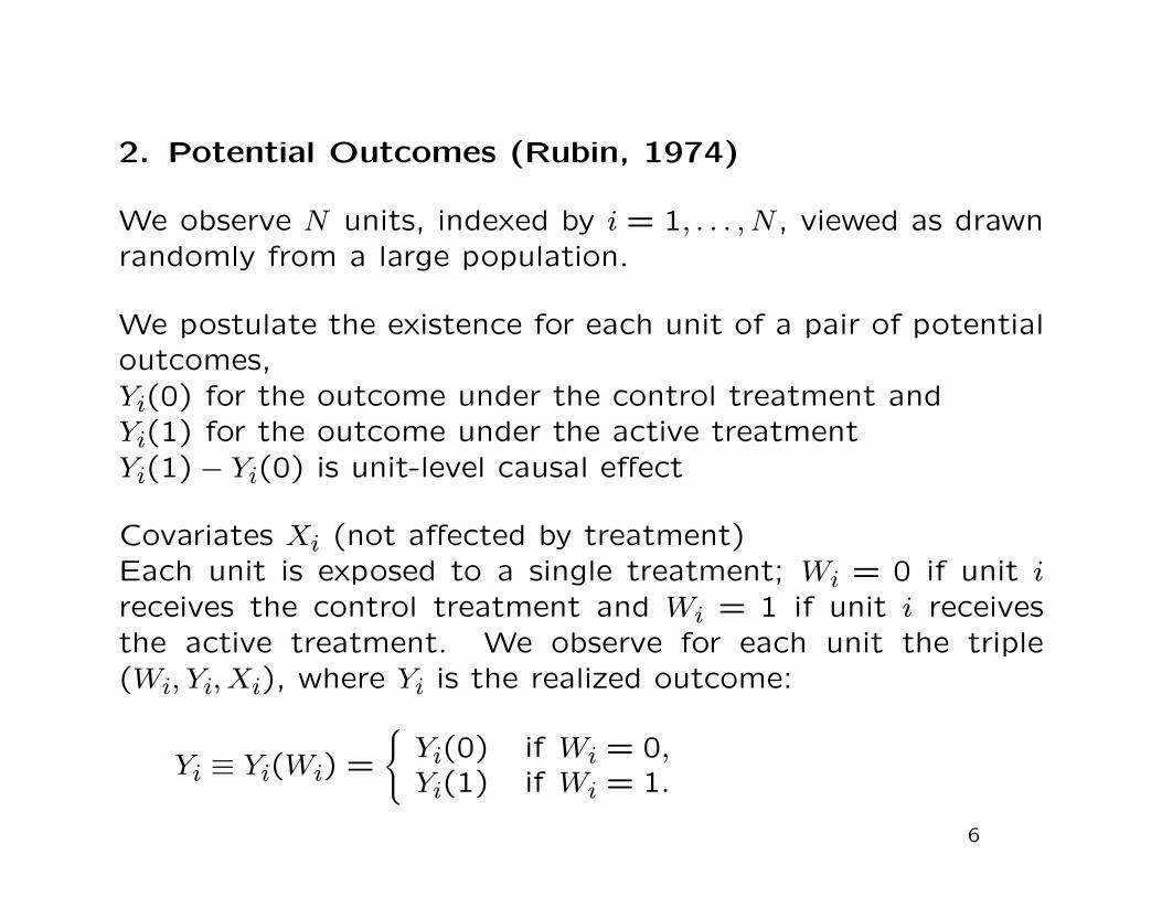
2. Potential Outcomes (Rubin, 1974)
We observe N units, indexed by i = 1, . . . , N , viewed as drawnrandomly from a large population.
We postulate the existence for each unit of a pair of potentialoutcomes,Yi(0) for the outcome under the control treatment andYi(1) for the outcome under the active treatmentYi(1) − Yi(0) is unit-level causal effect
Covariates Xi (not affected by treatment)Each unit is exposed to a single treatment; Wi = 0 if unit ireceives the control treatment and Wi = 1 if unit i receivesthe active treatment. We observe for each unit the triple(Wi, Yi, Xi), where Yi is the realized outcome:
Yi ≡ Yi(Wi) =
{Yi(0) if Wi = 0,Yi(1) if Wi = 1.
6

Several additional pieces of notation.
First, the propensity score (Rosenbaum and Rubin, 1983) is
defined as the conditional probability of receiving the treat-
ment,
e(x) = Pr(Wi = 1|Xi = x) = E[Wi|Xi = x].
Also the two conditional regression and variance functions:
μw(x) = E[Yi(w)|Xi = x], σ2w(x) = V(Yi(w)|Xi = x).
7

3. Estimands and Identification
Population average treatments
τP = E[Yi(1) − Yi(0)] τP,T = E[Yi(1)− Yi(0)|W = 1].
Most of the discussion in these notes will focus on τP , with
extensions to τP,T available in the references.
We will also look at the sample average treatment effect (SATE):
τS =1
N
N∑i=1
(Yi(1)− Yi(0))
τP versus τS does not matter for estimation, but matters for
variance.
8

4. Estimation and Inference
Assumption 1 (Unconfoundedness, Rosenbaum and Rubin, 1983a)
(Yi(0), Yi(1)) ⊥⊥ Wi | Xi.
“conditional independence assumption,” “selection on observ-ables.” In missing data literature “missing at random.”
To see the link with standard exogeneity assumptions, assumeconstant effect and linear regression:
Yi(0) = α + X′iβ + εi, =⇒ Yi = α + τ · Wi + X′
iβ + εi
with εi ⊥⊥ Xi. Given the constant treatment effect assumption,unconfoundedness is equivalent to independence of Wi and εi
conditional on Xi, which would also capture the idea that Wi
is exogenous.
9

Motivation for Unconfoundeness Assumption (I)
The first is a statistical, data descriptive motivation.
A natural starting point in the evaluation of any program is a
comparison of average outcomes for treated and control units.
A logical next step is to adjust any difference in average out-
comes for differences in exogenous background characteristics
(exogenous in the sense of not being affected by the treat-
ment).
Such an analysis may not lead to the final word on the efficacy
of the treatment, but the absence of such an analysis would
seem difficult to rationalize in a serious attempt to understand
the evidence regarding the effect of the treatment.
10

Motivation for Unconfoundeness Assumption (II)
A second argument is that almost any evaluation of a treatment
involves comparisons of units who received the treatment with
units who did not.
The question is typically not whether such a comparison should
be made, but rather which units should be compared, that is,
which units best represent the treated units had they not been
treated.
It is clear that settings where some of necessary covariates are
not observed will require strong assumptions to allow for iden-
tification. E.g., instrumental variables settings Absent those
assumptions, typically only bounds can be identified (e.g., Man-
ski, 1990, 1995).
11

Motivation for Unconfoundeness Assumption (III)
Example of a model that is consistent with unconfoundedness:suppose we are interested in estimating the average effect ofa binary input on a firm’s output, or Yi = g(W, εi).
Suppose that profits are output minus costs,
Wi = argmaxw
E[πi(w)|ci] = argmaxw
E[g(w, εi) − ci · w|ci],
implying
Wi = 1{E[g(1, εi) − g(0, εi) ≥ ci|ci]} = h(ci).
If unobserved marginal costs ci differ between firms, and thesemarginal costs are independent of the errors εi in the firms’forecast of output given inputs, then unconfoundedness willhold as
(g(0, εi), g(1, εi)) ⊥⊥ ci.
12

Overlap
Second assumption on the joint distribution of treatments and
covariates:
Assumption 2 (Overlap)
0 < Pr(Wi = 1|Xi) < 1.
Rosenbaum and Rubin (1983a) refer to the combination of the
two assumptions as ”stongly ignorable treatment assignment.”
13
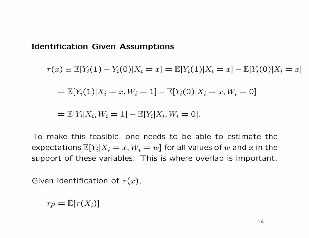
Identification Given Assumptions
τ(x) ≡ E[Yi(1)− Yi(0)|Xi = x] = E[Yi(1)|Xi = x] − E[Yi(0)|Xi = x]
= E[Yi(1)|Xi = x, Wi = 1] − E[Yi(0)|Xi = x, Wi = 0]
= E[Yi|Xi, Wi = 1] − E[Yi|Xi, Wi = 0].
To make this feasible, one needs to be able to estimate the
expectations E[Yi|Xi = x, Wi = w] for all values of w and x in the
support of these variables. This is where overlap is important.
Given identification of τ(x),
τP = E[τ(Xi)]
14

Alternative Assumptions
E[Yi(w)|Wi, Xi] = E[Yi(w)|Xi],
for w = 0,1. Although this assumption is unquestionably
weaker, in practice it is rare that a convincing case can be
made for the weaker assumption without the case being equally
strong for the stronger Assumption.
The reason is that the weaker assumption is intrinsically tied to
functional form assumptions, and as a result one cannot iden-
tify average effects on transformations of the original outcome
(e.g., logarithms) without the strong assumption.
If we are interested in τP,T it is sufficient to assume
Yi(0) ⊥⊥ Wi | Xi,
15

Propensity Score
Result 1 Suppose that Assumption 1 holds. Then:
(Yi(0), Yi(1)) ⊥⊥ Wi | e(Xi).
Only need to condition on scalar function of covariates, which
would be much easier in practice if Xi is high-dimensional.
(Problem is that the propensity score e(x) is almost never
known.)
16

Efficiency Bound
Hahn (1998): for any regular estimator for τP , denoted by τ ,
with
√N · (τ − τP )
d−→ N(0, V ),
the variance must satisfy:
V ≥ E
[σ21(Xi)
e(Xi)+
σ20(Xi)
1 − e(Xi)+ (τ(Xi)− τP )2
]. (1)
Estimators exist that achieve this bound.
17

Estimators
A. Regression Estimators
B. Matching
C. Propensity Score Estimators
D. Mixed Estimators (recommended)
18

A. Regression Estimators
Estimate μw(x) consistently and estimate τP or τS as
τreg =1
N
N∑i=1
(μ1(Xi) − μ0(Xi)).
Simple implementations include
μw(x) = β′x + τ · w,
in which case the average treatment effect is equal to τ . Inthis case one can estimate τ simply by least squares estimationusing the regression function
Yi = α + β′Xi + τ · Wi + εi.
More generally, one can specify separate regression functionsfor the two regimes, μw(x) = β′
wx.
19
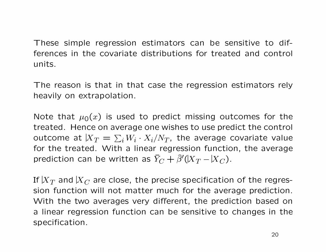
These simple regression estimators can be sensitive to dif-ferences in the covariate distributions for treated and controlunits.
The reason is that in that case the regression estimators relyheavily on extrapolation.
Note that μ0(x) is used to predict missing outcomes for thetreated. Hence on average one wishes to use predict the controloutcome at XT =
∑i Wi · Xi/NT , the average covariate value
for the treated. With a linear regression function, the averageprediction can be written as YC + β′(XT − XC).
If XT and XC are close, the precise specification of the regres-sion function will not matter much for the average prediction.With the two averages very different, the prediction based ona linear regression function can be sensitive to changes in thespecification.
20

−1 0 1 2 3 4 5 6 7 80
0.05
0.1
0.15
0.2
0.25
0.3
0.35
0.4
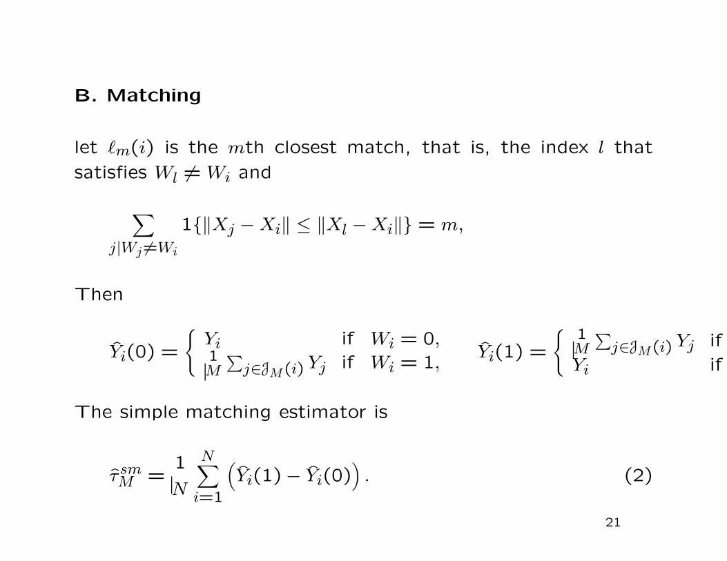
B. Matching
let �m(i) is the mth closest match, that is, the index l that
satisfies Wl = Wi and
∑j|Wj =Wi
1{‖Xj − Xi‖ ≤ ‖Xl − Xi‖} = m,
Then
Yi(0) =
{Yi if Wi = 0,1M
∑j∈JM(i) Yj if Wi = 1,
Yi(1) =
{1M
∑j∈JM(i) Yj if
Yi if
The simple matching estimator is
τ smM =
1
N
N∑i=1
(Yi(1)− Yi(0)
). (2)
21

Issues with Matching
Bias is of order O(N−1/K), where K is dimension of covariates.
Is important in large samples if K ≥ 2 (and dominates variance
asymptotically if K ≥ 3)
Not Efficient (but efficiency loss is small)
Easy to implement, robust.
22

C.1 Propensity Score Estimators: Weighting
E
[WY
e(X)
]= E
[E
[WYi(1)
e(X)
∣∣∣∣∣X]]
= E
[E
[e(X)Yi(1)
e(X)
]]= E[Yi(1)],
and similarly
E
[(1 − W )Y
1 − e(X)
]= E[Yi(0)],
implying
τP = E
[W · Ye(X)
− (1 − W ) · Y1 − e(X)
].
With the propensity score known one can directly implementthis estimator as
τ =1
N
N∑i=1
(Wi · Yi
e(Xi)− (1 − Wi) · Yi
1 − e(Xi)
). (3)
23

Implementation of Horvitz-Thompson Estimator
Estimate e(x) flexibly (Hirano, Imbens and Ridder, 2003)
τweight =N∑
i=1
Wi · Yi
e(Xi)/
N∑i=1
Wi
e(Xi)
−N∑
i=1
(1 − Wi) · Yi
1 − e(Xi)/
N∑i=1
(1 − Wi)
1 − e(Xi)
Is efficient given nonparametric estimator for e(x).
Potentially sensitive to estimator for propensity score.
24

Matching or Regression on the Propensity Score
Not clear what advantages are.
Large sample properties not known.
Simulation results not encouraging.
25
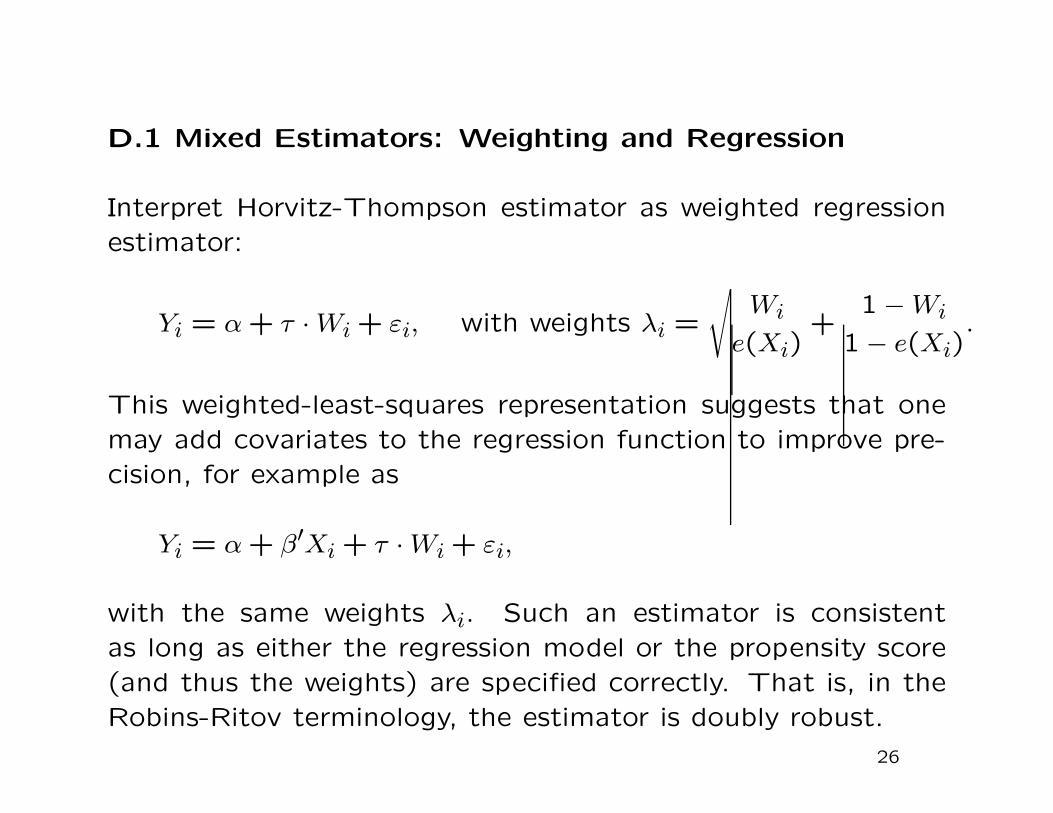
D.1 Mixed Estimators: Weighting and Regression
Interpret Horvitz-Thompson estimator as weighted regressionestimator:
Yi = α + τ · Wi + εi, with weights λi =
√Wi
e(Xi)+
1 − Wi
1 − e(Xi).
This weighted-least-squares representation suggests that onemay add covariates to the regression function to improve pre-cision, for example as
Yi = α + β′Xi + τ · Wi + εi,
with the same weights λi. Such an estimator is consistentas long as either the regression model or the propensity score(and thus the weights) are specified correctly. That is, in theRobins-Ritov terminology, the estimator is doubly robust.
26

Matching and Regression
First match observations.
Define
Xi(0) =
{Xi if Wi = 0,X�(i) if Wi = 1,
Xi(1) =
{X�(i) if Wi = 0,
Xi if Wi = 1.
Then adjust within pair difference for the within-pair differencein covariates Xi(1)− Xi(0):
τadjM =
1
N
N∑i=1
(Yi(1) − Yi(0) − β ·
(Xi(1)− Xi(0)
)),
using regression estimate for β.
Can eliminate bias of matching estimator given flexible speci-fication of regression function.
27
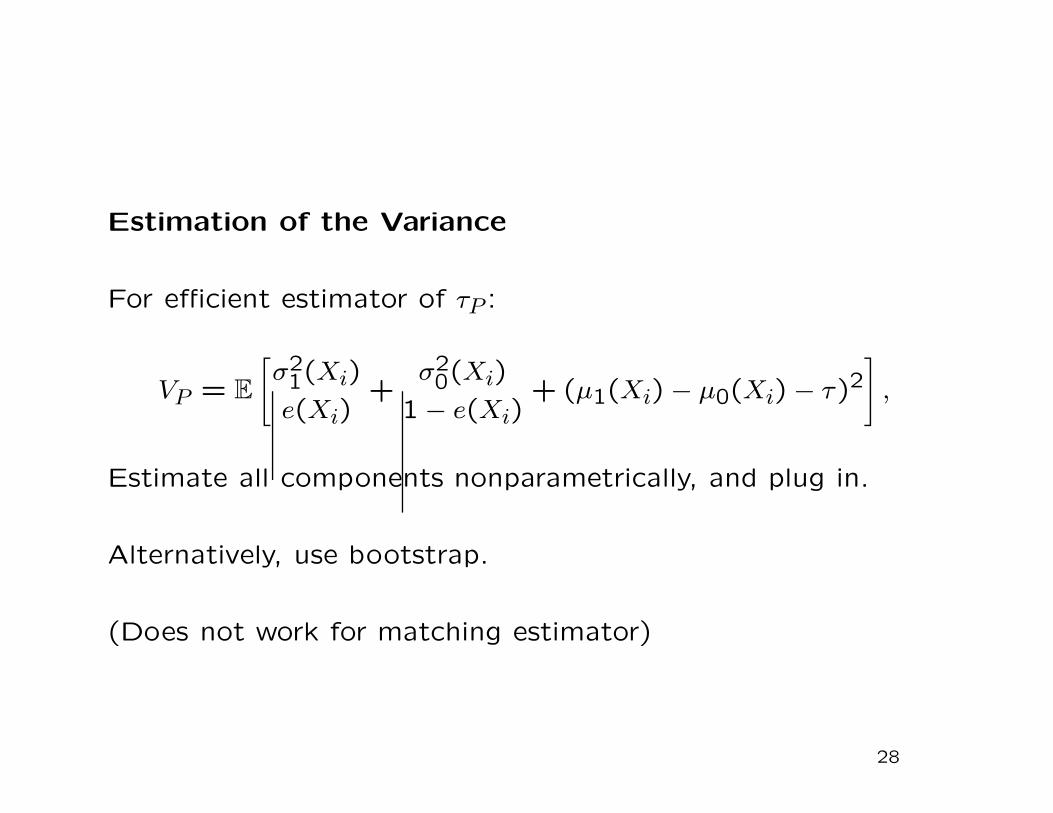
Estimation of the Variance
For efficient estimator of τP :
VP = E
[σ21(Xi)
e(Xi)+
σ20(Xi)
1 − e(Xi)+ (μ1(Xi) − μ0(Xi) − τ)2
],
Estimate all components nonparametrically, and plug in.
Alternatively, use bootstrap.
(Does not work for matching estimator)
28

Estimation of the Variance
For all estimators of τS, for some known λi(X,W)
τ =N∑
i=1
λi(X,W) · Yi,
V (τ |X, W) =N∑
i=1
λi(X, W)2 · σ2Wi
(Xi).
To estimate σ2Wi
(Xi) one uses the closest match within the setof units with the same treatment indicator. Let v(i) be theclosest unit to i with the same treatment indicator.
The sample variance of the outcome variable for these 2 unitscan then be used to estimate σ2
Wi(Xi):
σ2Wi
(Xi) =(Yi − Yv(i)
)2/2.
29
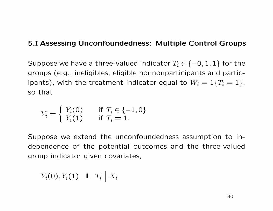
5.I Assessing Unconfoundedness: Multiple Control Groups
Suppose we have a three-valued indicator Ti ∈ {−0,1,1} for the
groups (e.g., ineligibles, eligible nonnonparticipants and partic-
ipants), with the treatment indicator equal to Wi = 1{Ti = 1},so that
Yi =
{Yi(0) if Ti ∈ {−1,0}Yi(1) if Ti = 1.
Suppose we extend the unconfoundedness assumption to in-
dependence of the potential outcomes and the three-valued
group indicator given covariates,
Yi(0), Yi(1) ⊥⊥ Ti
∣∣∣ Xi
30

Now a testable implication is
Yi(0) ⊥⊥ 1{Ti = 0}∣∣∣ Xi, Ti ∈ {−1,0},
and thus
Yi ⊥⊥ 1{Ti = 0}∣∣∣ Xi, Ti ∈ {−1,0}.
An implication of this independence condition is being tested
by the tests discussed above. Whether this test has much bear-
ing on the unconfoundedness assumption depends on whether
the extension of the assumption is plausible given unconfound-
edness itself.
31

5.II Assessing Unconfoundedness: Estimate Effects onPseudo Outcomes
Suppose the covariates consist of a number of lagged outcomesYi,−1, . . . , Yi,−T as well as time-invariant individual characteris-tics Zi, so that Xi = (Yi,−1, . . . , Yi,−T , Zi).
Now consider the following two assumptions. The first is un-confoundedness given only T − 1 lags of the outcome:
Yi,0(1), Yi,0(0) ⊥⊥ Wi | Yi,−1, . . . , Yi,−(T−1), Zi,
and the second assumes stationarity and exchangeability: Thenit follows that
Yi,−1 ⊥⊥ Wi | Yi,−2, . . . , Yi,−T , Zi,
which is testable.32

6.I Assessing Overlap
The first method to detect lack of overlap is to plot distribu-
tions of covariates by treatment groups. In the case with one
or two covariates one can do this directly. In high dimensional
cases, however, this becomes more difficult.
One can inspect pairs of marginal distributions by treatment
status, but these are not necessarily informative about lack of
overlap. It is possible that for each covariate the distribution
for the treatment and control groups are identical, even though
there are areas where the propensity score is zero or one.
A more direct method is to inspect the distribution of the
propensity score in both treatment groups, which can reveal
lack of overlap in the multivariate covariate distributions.
33

6.II Selecting a Subsample with Overlap
Define average effects for subsamples A:
τ(A) =N∑
i=1
1{Xi ∈ A} · τ(Xi)/N∑
i=1
1{Xi ∈ A}.
The efficiency bound for τ(A), assuming homoskedasticity, as
σ2
q(A)· E
[1
e(X)+
1
1 − e(X)
∣∣∣∣∣X ∈ A
],
where q(A) = Pr(X ∈ A).
They derive the characterization for the set A that minimizes
the asymptotic variance .
34

The optimal set has the form
A∗ = {x ∈ X|α ≤ e(X) ≤ 1 − α},
dropping observations with extreme values for the propensityscore, with the cutoff value α determined by the equation
1
α · (1 − α)=
2 · E
[1
e(X) · (1 − e(X))
∣∣∣∣∣ 1
e(X) · (1 − e(X))≤ 1
α · (1 − α)
].
Note that this subsample is selected solely on the basis of thejoint distribution of the treatment indicators and the covari-ates, and therefore does not introduce biases associated withselection based on the outcomes.
Calculations for Beta distributions for the propensity score sug-gest that α = 0.1 approximates the optimal set well in practice.
35
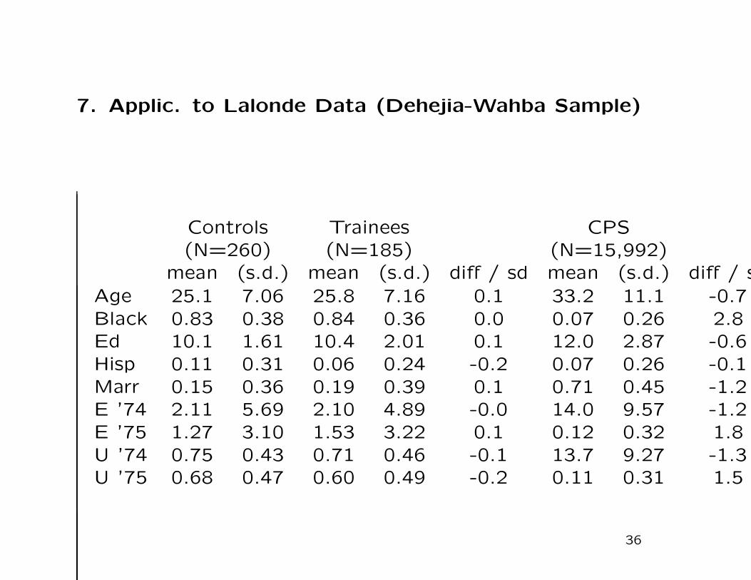
7. Applic. to Lalonde Data (Dehejia-Wahba Sample)
Controls Trainees CPS(N=260) (N=185) (N=15,992)
mean (s.d.) mean (s.d.) diff / sd mean (s.d.) diff / sAge 25.1 7.06 25.8 7.16 0.1 33.2 11.1 -0.7Black 0.83 0.38 0.84 0.36 0.0 0.07 0.26 2.8Ed 10.1 1.61 10.4 2.01 0.1 12.0 2.87 -0.6Hisp 0.11 0.31 0.06 0.24 -0.2 0.07 0.26 -0.1Marr 0.15 0.36 0.19 0.39 0.1 0.71 0.45 -1.2E ’74 2.11 5.69 2.10 4.89 -0.0 14.0 9.57 -1.2E ’75 1.27 3.10 1.53 3.22 0.1 0.12 0.32 1.8U ’74 0.75 0.43 0.71 0.46 -0.1 13.7 9.27 -1.3U ’75 0.68 0.47 0.60 0.49 -0.2 0.11 0.31 1.5
36

Table 2: Estimates for Lalonde Data with Earnings ’75 as Outcome
Experimental Controls CPS Comparison Groumean (s.e.) t-stat mean (s.e.) t-stat
Simple Dif 0.27 0.30 0.9 -12.12 0.68 -17.8OLS (parallel) 0.15 0.22 0.7 -1.15 0.36 -3.2OLS (separate) 0.12 0.22 0.6 -1.11 0.36 -3.1P Score Weighting 0.15 0.30 0.5 -1.17 0.26 -4.5P Score Blocking 0.10 0.17 0.6 -2.80 0.56 -5.0P Score Regression 0.16 0.30 0.5 -1.68 0.79 -2.1P Score Matching 0.23 0.37 0.6 -1.31 0.46 -2.9Matching 0.14 0.28 0.5 -1.33 0.41 -3.2Weighting and Regr 0.15 0.21 0.7 -1.23 0.24 -5.2Blocking and Regr 0.09 0.15 0.6 -1.30 0.50 -2.6Matching and Regr 0.06 0.28 0.2 -1.34 0.42 -3.2
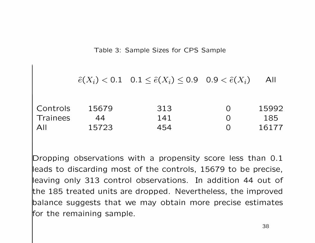
Table 3: Sample Sizes for CPS Sample
e(Xi) < 0.1 0.1 ≤ e(Xi) ≤ 0.9 0.9 < e(Xi) All
Controls 15679 313 0 15992Trainees 44 141 0 185All 15723 454 0 16177
Dropping observations with a propensity score less than 0.1
leads to discarding most of the controls, 15679 to be precise,
leaving only 313 control observations. In addition 44 out of
the 185 treated units are dropped. Nevertheless, the improved
balance suggests that we may obtain more precise estimates
for the remaining sample.
38

Table 4: Summary Statistics for Selected CPS Sample
Controls (N=313) Trainees (N=141)mean (s.d.) mean (s.d.) diff / sd
Age 26.60 10.97 25.69 7.29 -0.09Black 0.94 0.23 0.99 0.12 0.21Education 10.66 2.81 10.26 2.11 -0.15Hispanic 0.06 0.23 0.01 0.12 -0.21Married 0.22 0.42 0.13 0.33 -0.24Earnings ’74 1.96 4.08 1.34 3.72 -0.15Earnings ’75 0.57 0.50 0.80 0.40 0.49Unempl ’74 0.92 1.57 0.75 1.48 -0.11Unempl. ’75 0.55 0.50 0.69 0.46 0.28
39

Table 5: Estimates on Selected CPS Lalonde Data
Earn ’75 Outcome Earn ’78 Outcomemean (s.e.) t-stat mean (s.e.) t-stat
Simple Dif -0.17 0.16 -1.1 1.73 0.68 2.6OLS (parallel) -0.09 0.14 -0.7 2.10 0.71 3.0OLS (separate) -0.19 0.14 -1.4 2.18 0.72 3.0P Score Weighting -0.16 0.15 -1.0 1.86 0.75 2.5P Score Blocking -0.25 0.25 -1.0 1.73 1.23 1.4P Score Regression -0.07 0.17 -0.4 2.09 0.73 2.9P Score Matching -0.01 0.21 -0.1 0.65 1.19 0.5Matching -0.10 0.20 -0.5 2.10 1.16 1.8Weighting and Regr -0.14 0.14 -1.1 1.96 0.77 2.5Blocking and Regr -0.25 0.25 -1.0 1.73 1.22 1.4Matching and Regr -0.11 0.19 -0.6 2.23 1.16 1.9