Embed Size (px)
Citation preview
"Econometrics of Cross Section and Panel Data"
Lecture 1
Methods for Estimating Treatment Effects
Under Unconfoundedness, Part I
Guido Imbens
Cemmap Lectures, UCL, June 2014

1.A Introduction
Two applications where unconfoundedness/selection-on-observables
/exogeneity of treatment may be reasonable. How do we go
about analyzing these data?
• Summary Statistics
• Design: ensuring overlap
• Estimates of average treatment effects
• Assessing plausibility of unconfoundedness (should really be
done before estimation of average treatment effects)
2
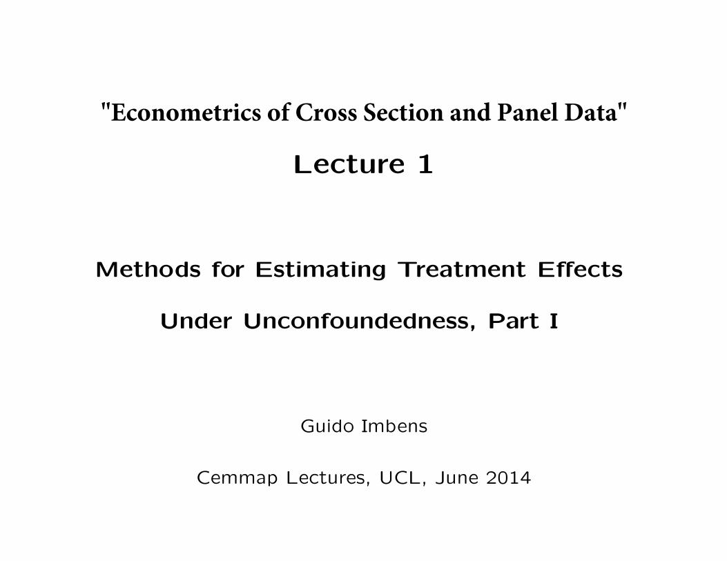
1.B outline
1. introduction/notation
2. description of applications and summary statistics
3. unconfoundedness
4. concerns with linear regression methods
5. design: assessing and ensuring overlap
6. estimation of average treatment effects
7. assessing unconfoundedness
3
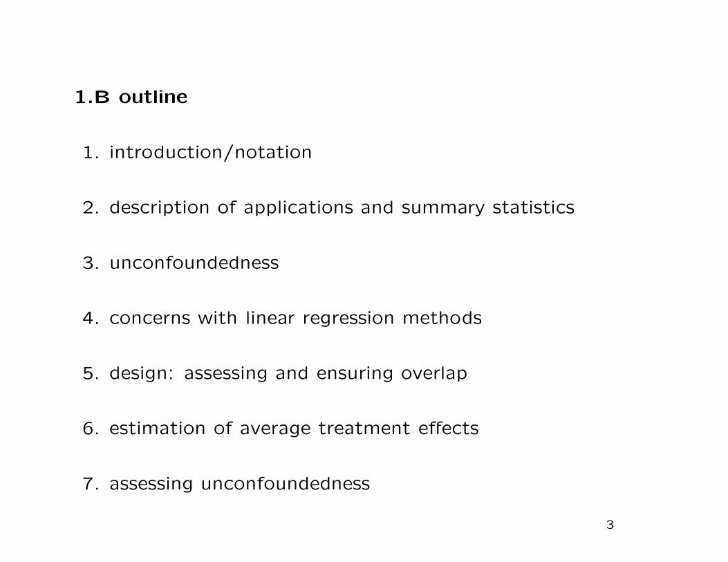
1.C Notation
Treatment indicator: Wi
Potential Outcomes Yi(0), Yi(1)
Covariates Xi
Observed outcome: Y obsi = Wi · Yi(1) + (1 − Wi) · Yi(0).
Nc =∑
(1 − Wi) number of controls, Nt =∑
i Wi number of
treated units.
Yobsc and Y
obst are average outcomes for controls and treated.
4

2. Application I: Imbens-Rubin-Sacerdote Lottery Study
IRS were interested in estimating the effect of unearned in-
come on economic behavior including effects on labor supply,
consumption and savings.
Those effects are important to understand and improve design
of social security programs.
IRS surveyed individuals who had played and won large sums of
money in the lottery (“winners”). As a comparison group they
collected data on a second set of individuals who also played
the lottery but who had not won big prizes (the “losers”) .
5

Nt = 259 winners and Nc = 237 losers in the sample of N = 496
lottery players.
We know the year individuals played the lottery, the number of
tickets they typically bought, age, sex, education, and their so-
cial security earnings for the six years preceeding their winning.
(what else should we have asked for?)
We present averages and standard deviations for the full sam-
ple, t-statistics for the null hypothesis of equal means in the
two groups, and the normalized differences in the means.
6

Normalized Difference in Covariates
Xc =1
Nc
∑
i:Wi=0
Xi S2c =
1
Nc − 1
∑
i:Wi=0
(
Xi − Xc
)2
Xt =1
Nt
∑
i:Wi=1
Xi S2t =
1
Nt − 1
∑
i:Wi=1
(
Xi − Xt
)2
Normalized difference:
nd =Xt − Xc
√
(S2c + S2
t )/2
More relevant for assessing balance than the t-statistic
t =Xt − Xc
√
S2c /Nc + S2
t /Nt
7

Summary Statistics Lottery Sample
Variable All Losers WinnersN=496 Nt=259 Nc=237 Norm.
mean (s.d.) mean mean [t-stat] Dif.
Year Won 6.23 1.18 6.38 6.06 -3.0 -0.27# Tickets 3.33 2.86 2.19 4.57 9.9 0.90Age 50.2 13.7 53.2 47.0 -5.2 -0.47Male 0.63 0.48 0.67 0.58 -2.1 -0.19Education 13.73 2.20 14.43 12.97 -7.8 -0.70Working Then 0.78 0.41 0.77 0.80 0.9 0.08Earn Y -6 13.8 13.4 15.6 12.0 -3.1 -0.27...Earn Y -1 16.3 15.7 18.0 14.5 -2.5 -0.23Pos Earn Y-6 0.69 0.46 0.69 0.70 0.3 0.03...Pos Earn Y-1 0.71 0.45 0.69 0.74 1.2 0.10
8
There are substantial differences between the two groups, in-
cluding in pre-winning earnings and the number of lottery tick-
ets bought. This suggests that simple regression methods will
not necessarily be adequate for removing the biases associated
with the differences in covariates.
Where do these differences come from?
• People buying more tickets are more likely to win.
• Nonresponse may differ by prize and individual characteris-
tics (including labor income)
Is unconfoundedness plausible?
9

Application II: Lalonde Study
Lalonde (1986) analyzed data from a randomized experiment
designed to evaluate the effect of a labor market program, the
National Supported Work (NSW) program.
Women with poor labor market histories.
Randomized evaluation shows average effect on earnings
≈ $2,000. (Substantial for participants).
Lalonde: could we have estimated this without random-
ized experiment?
10

Lalonde Evaluation of the Effectiveness of Observational
Methods to Recover Causal Effects:
Put aside experimental control group.
Constructs comparison sample from public use data set: Cur-
rent Population Survey (CPS), and Panel Study of Income
Dynamics (PSID).
Estimate average effect using CPS (or PSID) and trainees, as
observational study.
Is estimated effect close to experimental estimate?
Lalonde concludes that nonexperimental evaluations are
not credible. Influential conclusion in policy circles.
11
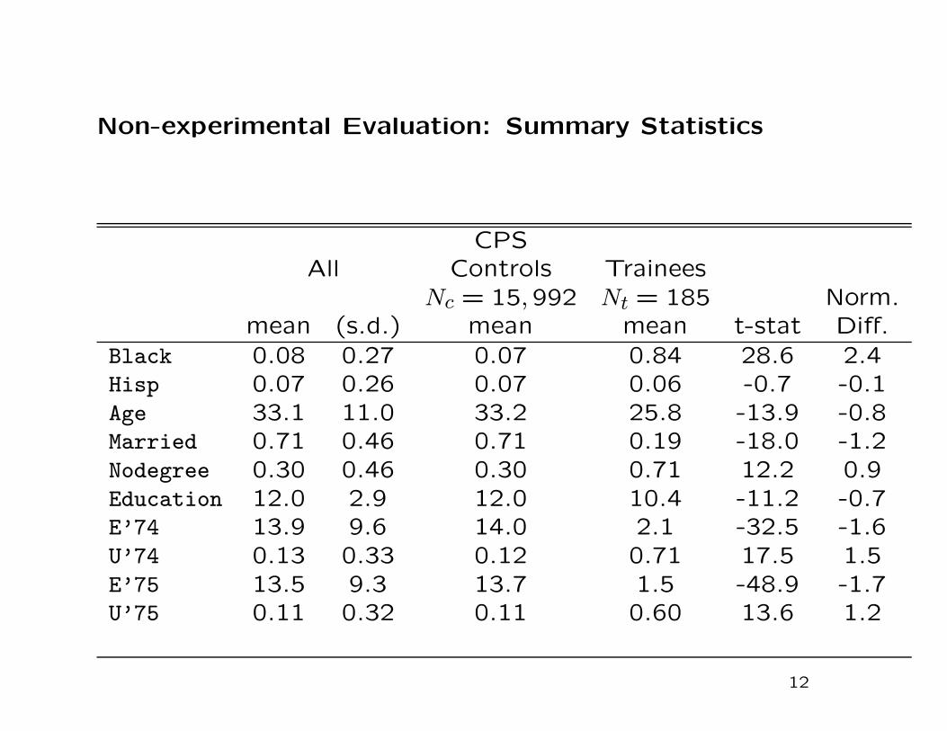
Non-experimental Evaluation: Summary Statistics
CPSAll Controls Trainees
Nc = 15,992 Nt = 185 Norm.mean (s.d.) mean mean t-stat Diff.
Black 0.08 0.27 0.07 0.84 28.6 2.4Hisp 0.07 0.26 0.07 0.06 -0.7 -0.1Age 33.1 11.0 33.2 25.8 -13.9 -0.8Married 0.71 0.46 0.71 0.19 -18.0 -1.2Nodegree 0.30 0.46 0.30 0.71 12.2 0.9Education 12.0 2.9 12.0 10.4 -11.2 -0.7E’74 13.9 9.6 14.0 2.1 -32.5 -1.6U’74 0.13 0.33 0.12 0.71 17.5 1.5E’75 13.5 9.3 13.7 1.5 -48.9 -1.7U’75 0.11 0.32 0.11 0.60 13.6 1.2
12

3. Assumptions
I. Unconfoundedness
Yi(0), Yi(1) ⊥ Wi
∣
∣
∣
∣
Xi.
This form due to Rosenbaum and Rubin (1983). Sometimes
referred to as “selection on observables”, or “exogeneity” but
those terms are not well defined.
Suppose
Yi(0) = α + β′Xi + εi, and Yi(1) = Yi(0) + τ,
then
Yi = α + τ · Wi + β′Xi + εi,
and unconfoundedness ⇐⇒ εi ⊥ Wi|Xi (exogeneity)
13
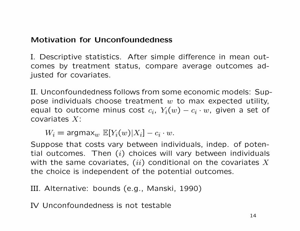
Motivation for Unconfoundedness
I. Descriptive statistics. After simple difference in mean out-comes by treatment status, compare average outcomes ad-justed for covariates.
II. Unconfoundedness follows from some economic models: Sup-pose individuals choose treatment w to max expected utility,equal to outcome minus cost ci, Yi(w) − ci · w, given a set ofcovariates X:
Wi = argmaxw E[Yi(w)|Xi]− ci · w.
Suppose that costs vary between individuals, indep. of poten-tial outcomes. Then (i) choices will vary between individualswith the same covariates, (ii) conditional on the covariates Xthe choice is independent of the potential outcomes.
III. Alternative: bounds (e.g., Manski, 1990)
IV Unconfoundedness is not testable
14

II. Overlap
0 < pr(Wi = 1|Xi) < 1.
For all X there are treated and control units.
This assumption is in principle testable: one can estimate the
propensity score
e(x) = pr(Wi = 1|Xi = x)
and assess whether it gets close to zero.
I and II combined: Strong Ignorability (Rosenbaum and Rubin,
1983)
This is what we will work with for these two applications.
15
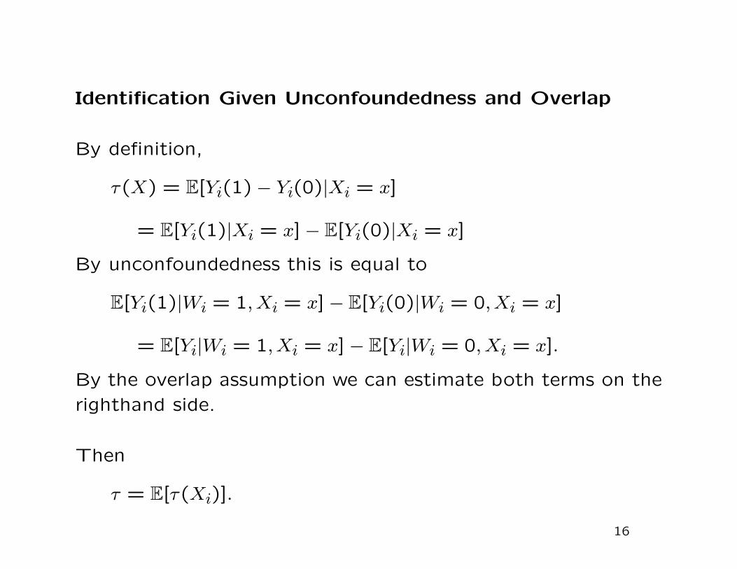
Identification Given Unconfoundedness and Overlap
By definition,
τ(X) = E[Yi(1) − Yi(0)|Xi = x]
= E[Yi(1)|Xi = x] − E[Yi(0)|Xi = x]
By unconfoundedness this is equal to
E[Yi(1)|Wi = 1, Xi = x] − E[Yi(0)|Wi = 0,Xi = x]
= E[Yi|Wi = 1,Xi = x] − E[Yi|Wi = 0, Xi = x].
By the overlap assumption we can estimate both terms on the
righthand side.
Then
τ = E[τ(Xi)].
16

4. Concern with regression estimators in cases with lim-
ited overlap in covariate distributions (distinct from plausi-
bility of unconfoundedness assumption)
Regression estimators are the most widely used methods for
estimating treatment effects
Sometimes simple linear regression:
Y obsi = β0 + τ · Wi + β1 · Xi + ε
Sometimes allowing for interactions:
Y obsi = β0 + τ · Wi + β1 · Xi + β2 · (Xi − X) · Wi + ε
What is the problem with these methods?
17
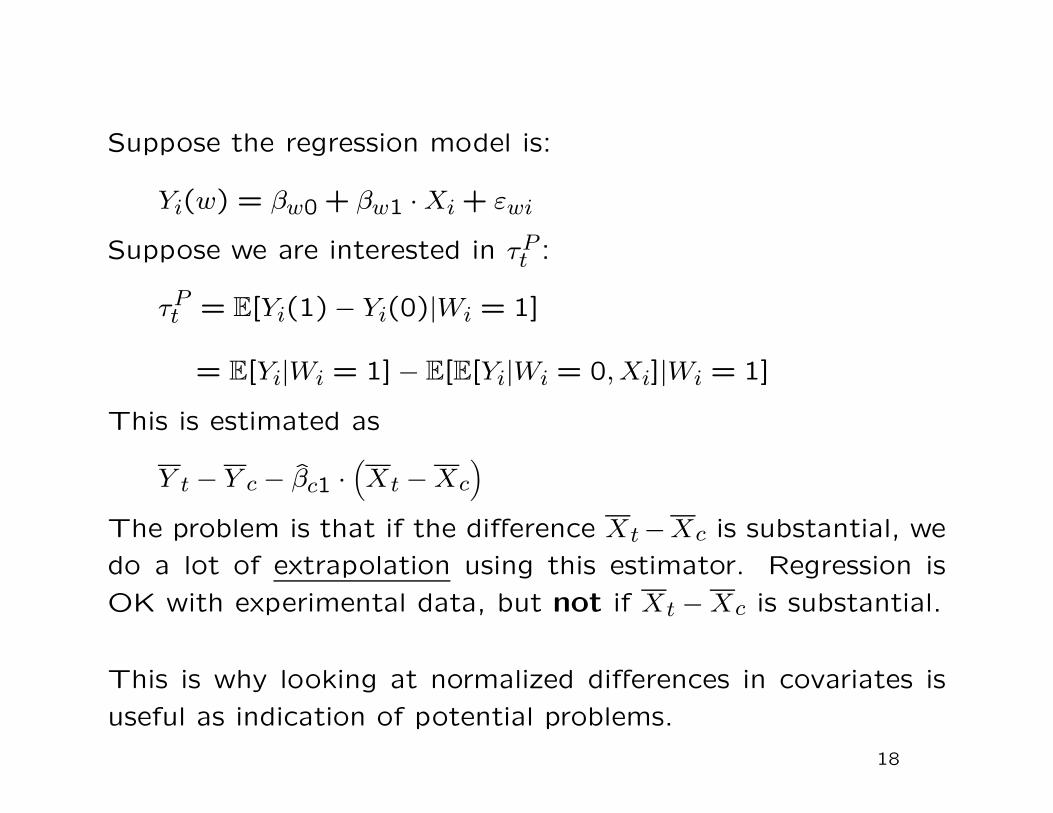
Suppose the regression model is:
Yi(w) = βw0 + βw1 · Xi + εwi
Suppose we are interested in τPt :
τPt = E[Yi(1)− Yi(0)|Wi = 1]
= E[Yi|Wi = 1] − E[E[Yi|Wi = 0, Xi]|Wi = 1]
This is estimated as
Y t − Y c − βc1 ·(
Xt − Xc
)
The problem is that if the difference Xt−Xc is substantial, we
do a lot of extrapolation using this estimator. Regression is
OK with experimental data, but not if Xt − Xc is substantial.
This is why looking at normalized differences in covariates is
useful as indication of potential problems.
18
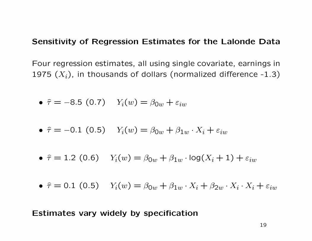
Sensitivity of Regression Estimates for the Lalonde Data
Four regression estimates, all using single covariate, earnings in
1975 (Xi), in thousands of dollars (normalized difference -1.3)
• τ = −8.5 (0.7) Yi(w) = β0w + εiw
• τ = −0.1 (0.5) Yi(w) = β0w + β1w · Xi + εiw
• τ = 1.2 (0.6) Yi(w) = β0w + β1w · log(Xi + 1) + εiw
• τ = 0.1 (0.5) Yi(w) = β0w + β1w · Xi + β2w · Xi · Xi + εiw
Estimates vary widely by specification
19
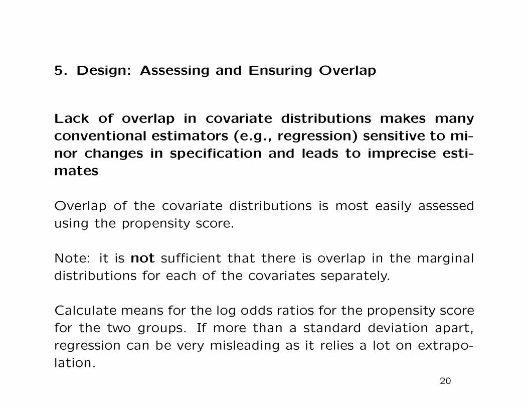
5. Design: Assessing and Ensuring Overlap
Lack of overlap in covariate distributions makes many
conventional estimators (e.g., regression) sensitive to mi-
nor changes in specification and leads to imprecise esti-
mates
Overlap of the covariate distributions is most easily assessed
using the propensity score.
Note: it is not sufficient that there is overlap in the marginal
distributions for each of the covariates separately.
Calculate means for the log odds ratios for the propensity score
for the two groups. If more than a standard deviation apart,
regression can be very misleading as it relies a lot on extrapo-
lation.
20
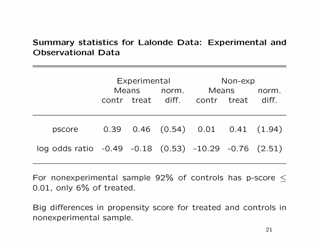
Summary statistics for Lalonde Data: Experimental and
Observational Data
Experimental Non-expMeans norm. Means norm.
contr treat diff. contr treat diff.
pscore 0.39 0.46 (0.54) 0.01 0.41 (1.94)
log odds ratio -0.49 -0.18 (0.53) -10.29 -0.76 (2.51)
For nonexperimental sample 92% of controls has p-score ≤
0.01, only 6% of treated.
Big differences in propensity score for treated and controls in
nonexperimental sample.
21

Two Alternatives in Case with Limited Overlap:
Under unconfoundedness, if overlap in covariates between treated
and controls is limited, the population average treatment effect
is difficult to estimate.
• Create matched sample to estimate average effect on treated.
• Create subsample with overlap.
22
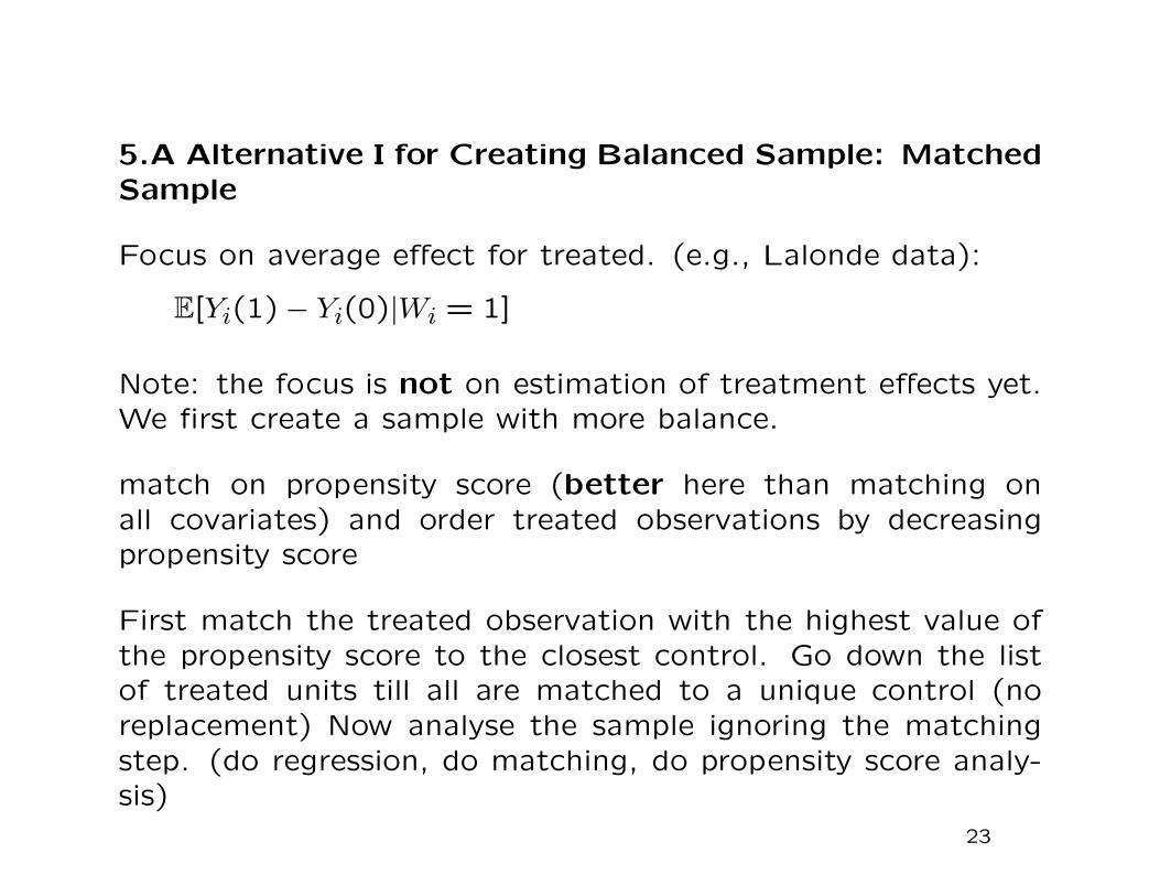
5.A Alternative I for Creating Balanced Sample: MatchedSample
Focus on average effect for treated. (e.g., Lalonde data):
E[Yi(1)− Yi(0)|Wi = 1]
Note: the focus is not on estimation of treatment effects yet.We first create a sample with more balance.
match on propensity score (better here than matching onall covariates) and order treated observations by decreasingpropensity score
First match the treated observation with the highest value ofthe propensity score to the closest control. Go down the listof treated units till all are matched to a unique control (noreplacement) Now analyse the sample ignoring the matchingstep. (do regression, do matching, do propensity score analy-sis)
23

Matching to Improve Balance
We first estimate the propensity score, using the 185 trainees
and 15,992 CPS controls.
Then we order the 185 trainees by the estimated propensity
score, the largest first.
Then, going down the list of trainees, we match each to the
nearest CPS control, in terms of the estimated propensity
score, without replacement.
Now we have a new data set with 185 treated and 185 matched
CPS controls.
Balance is much improved.
24
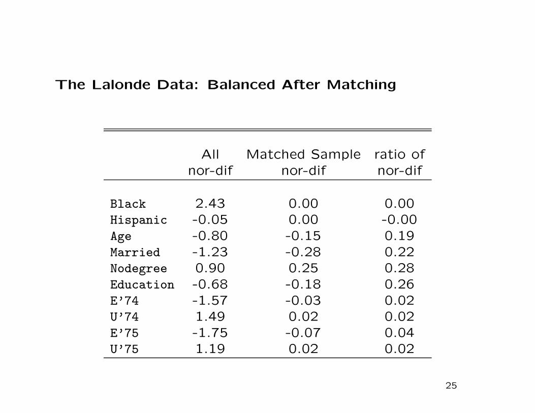
The Lalonde Data: Balanced After Matching
All Matched Sample ratio ofnor-dif nor-dif nor-dif
Black 2.43 0.00 0.00Hispanic -0.05 0.00 -0.00Age -0.80 -0.15 0.19Married -1.23 -0.28 0.22Nodegree 0.90 0.25 0.28Education -0.68 -0.18 0.26E’74 -1.57 -0.03 0.02U’74 1.49 0.02 0.02E’75 -1.75 -0.07 0.04U’75 1.19 0.02 0.02
25
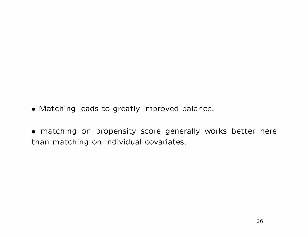
• Matching leads to greatly improved balance.
• matching on propensity score generally works better here
than matching on individual covariates.
26
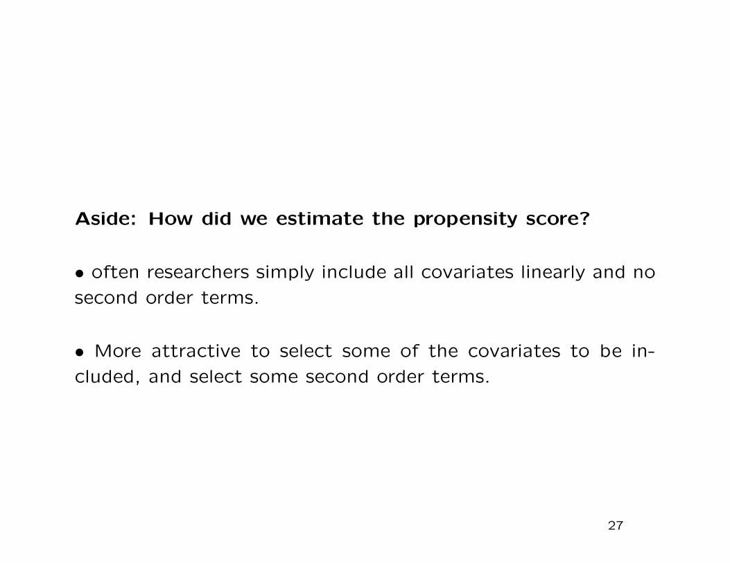
Aside: How did we estimate the propensity score?
• often researchers simply include all covariates linearly and no
second order terms.
• More attractive to select some of the covariates to be in-
cluded, and select some second order terms.
27
Specification Search
Given K covariates, we first choose a subset of the K covariates
for linear inclusion in the propensity score, and in a second
step we selection subset of all second order terms involving the
covariates that are selected in the first step.
Limitation: we only include linear, quadratic and interaction
terms, no third order terms (rarely substantitively important).
Sequential selection of covariates based on likelihood ratio test
and repeated estimation of logistic regression model. (see IR
book for details)
Other algorithms possible, e.g., lasso.
28
5.B Design Option II: Trimming the Sample
Traditional Estimand
τP = E[Yi(1)− Yi(0)] = E[τ(Xi)] (Population Average Treat-
ment Effect)
Problem:
τP can be difficult to estimate when there are values x ∈ X
such that e(x) close to zero or one.
• estimates are imprecise (high variance)
• estimates are sensitive to small changes in specification
29
Previous Solutions:
I Dehejia & Wahba (1999): Drop control units i with e(Xi) <
minj:Wj=1 e(Xj). Generalization (Lechner): discard all con-
trol units with e(Xi) smaller than kth smallest propensity score
among treated.
II Heckman, Ichimura, Todd (1998): Estimate f0(x) = f(X|W =
0), f1(x) = f(X|W = 1). Drop unit i if f0(Xi) ≤ q0 or
f1(Xi) ≤ q1, where q0 and q1 are quantiles of the distribution
of f0(X) and f1(X) respectively.
Both are ad hoc, and potentially sensitive to choice of threshold
(k for DW, q0 and q1 in HIT).
30
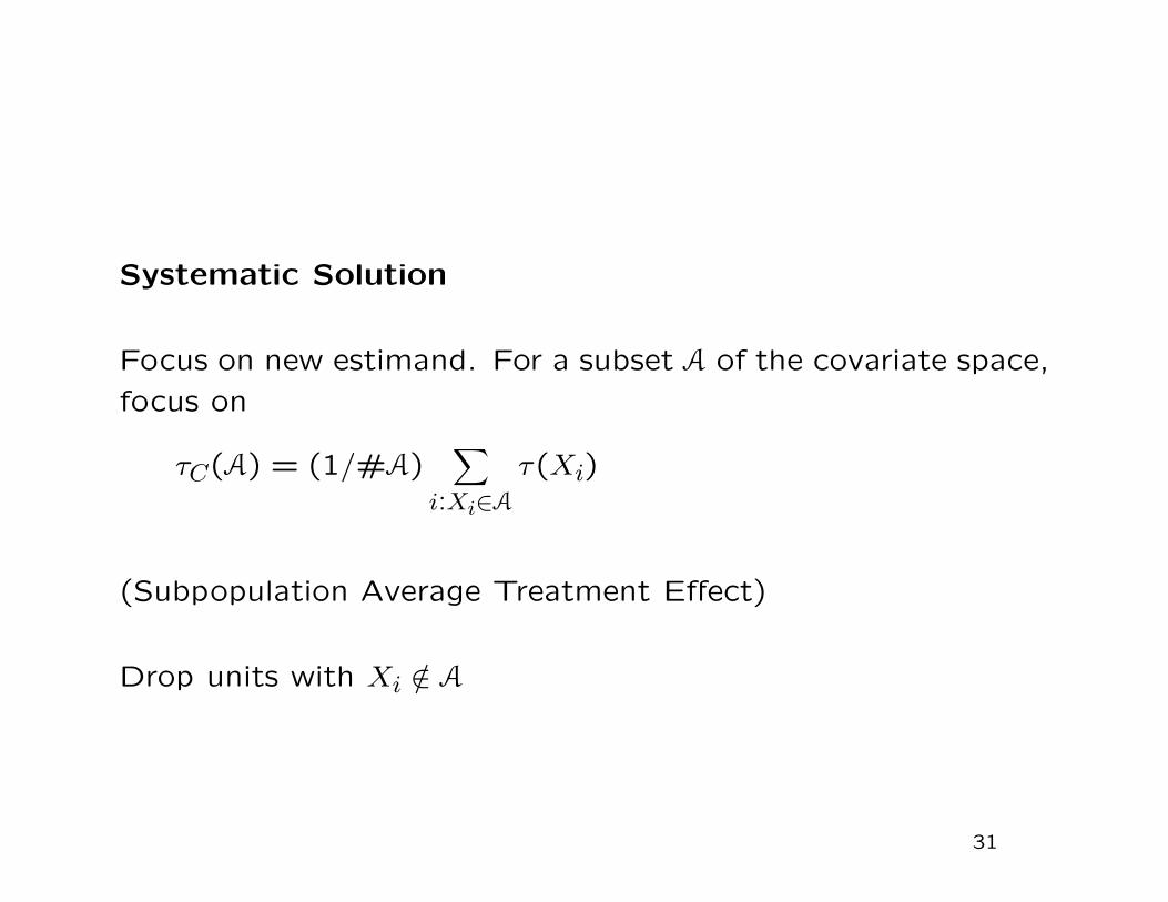
Systematic Solution
Focus on new estimand. For a subset A of the covariate space,
focus on
τC(A) = (1/#A)∑
i:Xi∈A
τ(Xi)
(Subpopulation Average Treatment Effect)
Drop units with Xi /∈ A
31
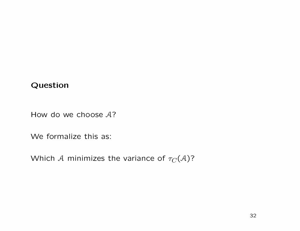
Question
How do we choose A?
We formalize this as:
Which A minimizes the variance of τC(A)?
32
Illustration: Binary X Case
X ∈ f, m
Nx is sample size for the subsample with X = x
p = Nm/N be the population share of X = 1 units.
τx is average treatment effect conditional on the covariate
τ = p · τm + (1 − p) · τf . Nxw is number of observations with
covariate Xi = x and treatment indicator Wi = w.
ex = Nxt/Nx is propensity score for x = f, m.
Y cx =∑
i:Wi=0,Xi=x Yi/Nxc, Y tx =∑
i:Wi=1,Xi=x Yi/Nxt
Assume that the variance of Yi(w) given Xi = x is σ2 for all x.
33

τx = Y tx − Y cx
with variances
V (τf) =σ2
N · (1 − p)·
1
ef · (1 − ef),
V (τm) =σ2
N · p·
1
em · (1 − em),
The estimator for the population average treatment effect is
τ = p · τm + (1 − p) · τf .
with variance
V (τ) =σ2
N· E
[
1
eX · (1 − eX)
]
.
34
Define V = min(V (τ), V (τf), V (τm). Then
V =
V (τf) if em(1−em)ef(1−ef)
≤ 1−p2−p,
V (τ) if 1−p2−p ≤ em(1−em)
ef(1−ef)≤ 1+p
p ,
V (τm) if 1+pp ≤ em(1−em)
ef(1−ef).
If ef is close to zero or one, we may be better of focusing on
τm, and the other way around. If both are far from zero and
one, we can focus on τ .
“Better off” here means that we can estimate the correspond-
ing estimand more accurately.
35
General Case
Optimal set:
A = x ∈ X |α < e(x) < 1 − α ,
where α depends on the distribution of the propensity score
in the sample. (See Crump, Hotz, Imbens, Mitnik, Biometrika
2009)
Approximate solution:
A∗ = x ∈ X |0.1 < e(x) < 0.9
Practical recommendation: drop units with a propensity
score below 0.1 or above 0.9.
36
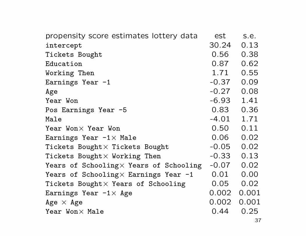
propensity score estimates lottery data est s.e.intercept 30.24 0.13Tickets Bought 0.56 0.38Education 0.87 0.62Working Then 1.71 0.55Earnings Year -1 -0.37 0.09Age -0.27 0.08Year Won -6.93 1.41Pos Earnings Year -5 0.83 0.36Male -4.01 1.71Year Won× Year Won 0.50 0.11Earnings Year -1× Male 0.06 0.02Tickets Bought× Tickets Bought -0.05 0.02Tickets Bought× Working Then -0.33 0.13Years of Schooling× Years of Schooling -0.07 0.02Years of Schooling× Earnings Year -1 0.01 0.00Tickets Bought× Years of Schooling 0.05 0.02Earnings Year -1× Age 0.002 0.001Age × Age 0.002 0.001Year Won× Male 0.44 0.25
37
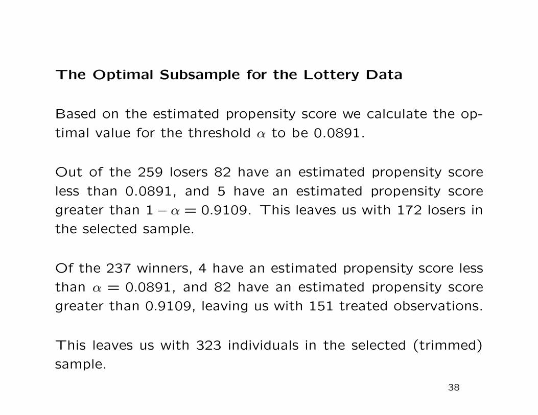
The Optimal Subsample for the Lottery Data
Based on the estimated propensity score we calculate the op-
timal value for the threshold α to be 0.0891.
Out of the 259 losers 82 have an estimated propensity score
less than 0.0891, and 5 have an estimated propensity score
greater than 1− α = 0.9109. This leaves us with 172 losers in
the selected sample.
Of the 237 winners, 4 have an estimated propensity score less
than α = 0.0891, and 82 have an estimated propensity score
greater than 0.9109, leaving us with 151 treated observations.
This leaves us with 323 individuals in the selected (trimmed)
sample.
38
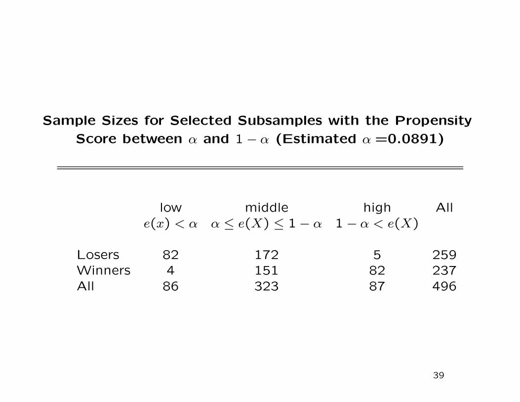
Sample Sizes for Selected Subsamples with the Propensity
Score between α and 1 − α (Estimated α =0.0891)
low middle high Alle(x) < α α ≤ e(X) ≤ 1 − α 1 − α < e(X)
Losers 82 172 5 259Winners 4 151 82 237All 86 323 87 496
39
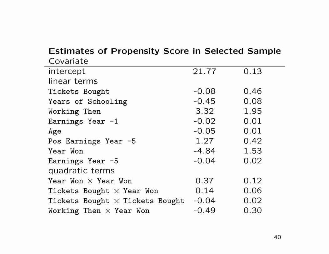
Estimates of Propensity Score in Selected SampleCovariate
intercept 21.77 0.13linear termsTickets Bought -0.08 0.46Years of Schooling -0.45 0.08Working Then 3.32 1.95Earnings Year -1 -0.02 0.01Age -0.05 0.01Pos Earnings Year -5 1.27 0.42Year Won -4.84 1.53Earnings Year -5 -0.04 0.02quadratic termsYear Won × Year Won 0.37 0.12Tickets Bought × Year Won 0.14 0.06Tickets Bought × Tickets Bought -0.04 0.02Working Then × Year Won -0.49 0.30
40

"Econometrics of Cross Section and Panel Data"
Lecture 2
Methods for Estimating Treatment Effects
Under Unconfoundedness, Part II
Guido Imbens
Cemmap Lectures, UCL, June 2014
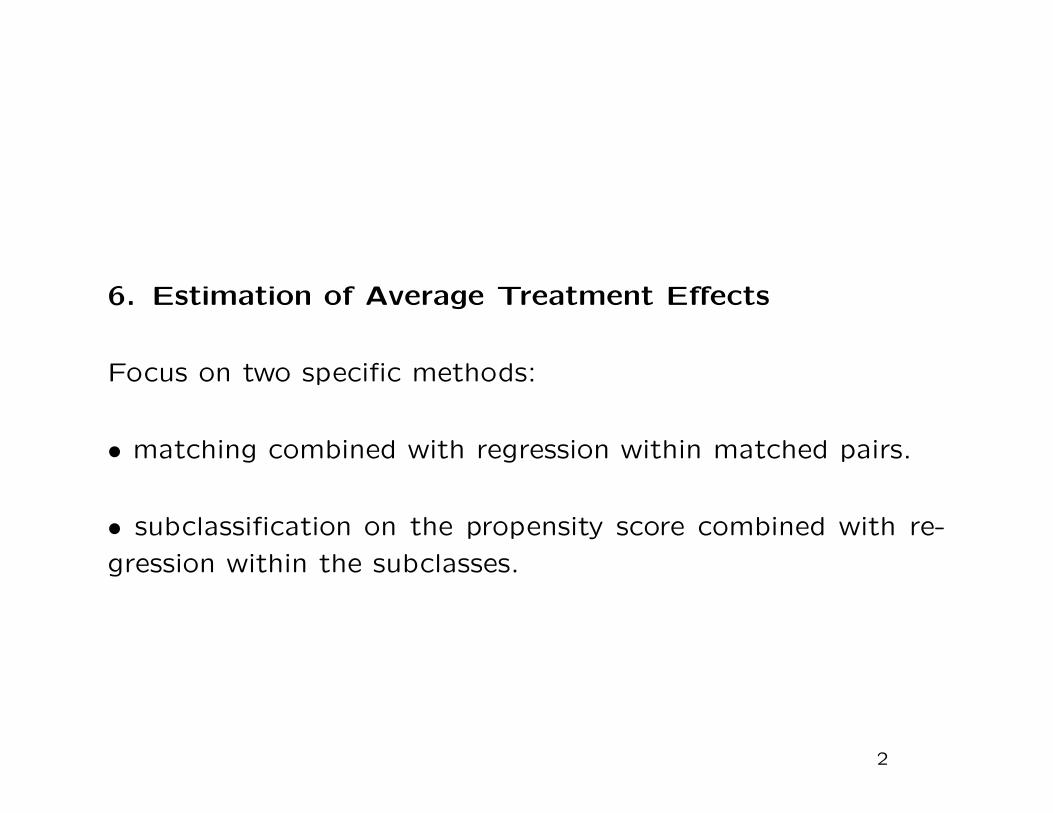
6. Estimation of Average Treatment Effects
Focus on two specific methods:
• matching combined with regression within matched pairs.
• subclassification on the propensity score combined with re-
gression within the subclasses.
2
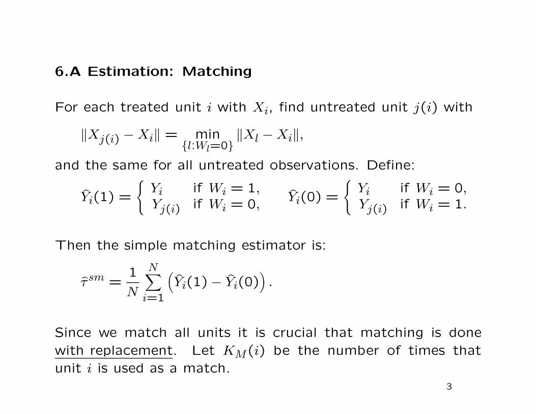
6.A Estimation: Matching
For each treated unit i with Xi, find untreated unit j(i) with
‖Xj(i) − Xi‖ = minl:Wl=0
‖Xl − Xi‖,
and the same for all untreated observations. Define:
Yi(1) =
Yi if Wi = 1,Yj(i) if Wi = 0,
Yi(0) =
Yi if Wi = 0,Yj(i) if Wi = 1.
Then the simple matching estimator is:
τsm =1
N
N∑
i=1
(Yi(1)− Yi(0)
).
Since we match all units it is crucial that matching is done
with replacement. Let KM(i) be the number of times that
unit i is used as a match.
3
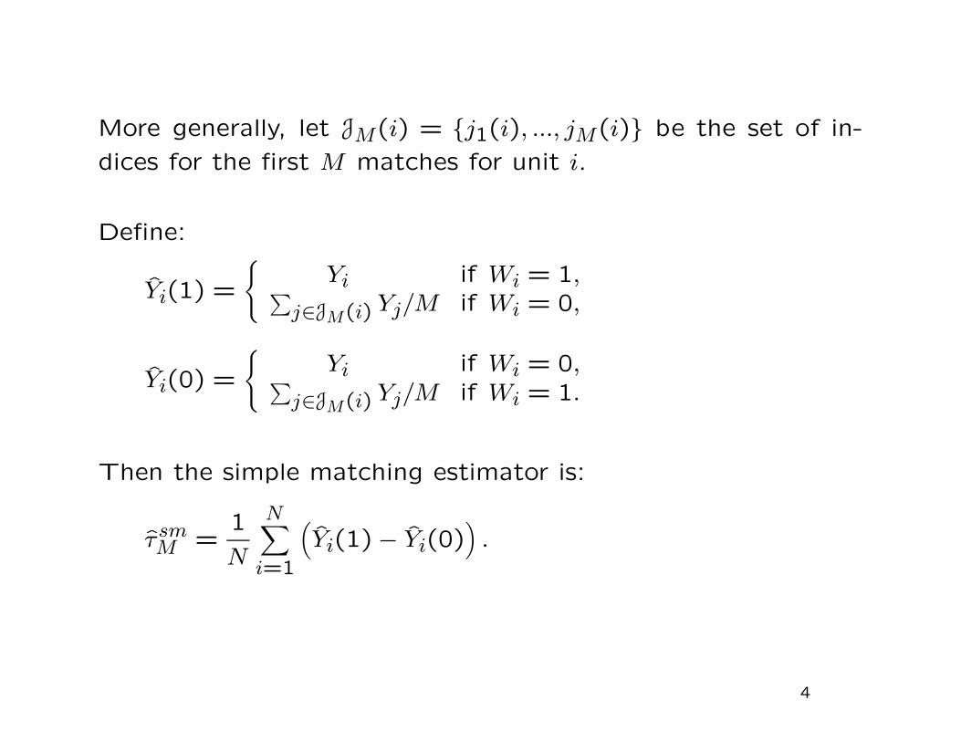
More generally, let JM(i) = j1(i), ..., jM(i) be the set of in-
dices for the first M matches for unit i.
Define:
Yi(1) =
Yi if Wi = 1,∑
j∈JM(i) Yj/M if Wi = 0,
Yi(0) =
Yi if Wi = 0,∑
j∈JM(i) Yj/M if Wi = 1.
Then the simple matching estimator is:
τsmM =
1
N
N∑
i=1
(Yi(1)− Yi(0)
).
4
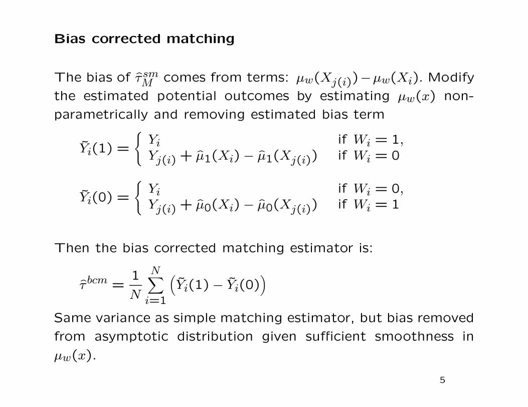
Bias corrected matching
The bias of τsmM comes from terms: µw(Xj(i))−µw(Xi). Modify
the estimated potential outcomes by estimating µw(x) non-
parametrically and removing estimated bias term
Yi(1) =
Yi if Wi = 1,Yj(i) + µ1(Xi) − µ1(Xj(i)) if Wi = 0
Yi(0) =
Yi if Wi = 0,Yj(i) + µ0(Xi) − µ0(Xj(i)) if Wi = 1
Then the bias corrected matching estimator is:
τ bcm =1
N
N∑
i=1
(Yi(1) − Yi(0)
)
Same variance as simple matching estimator, but bias removed
from asymptotic distribution given sufficient smoothness in
µw(x).
5

Variance of Matching Estimators
The variance of τsmM conditional on W and X, normalized by
the sample size N , is
1
N
N∑
i=1
(
1 +KM(i)
M
)2
· σ2Wi
(Xi).
6
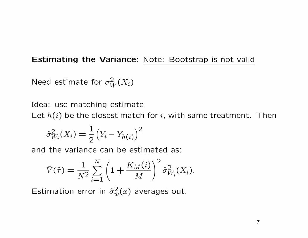
Estimating the Variance: Note: Bootstrap is not valid
Need estimate for σ2W (Xi)
Idea: use matching estimate
Let h(i) be the closest match for i, with same treatment. Then
σ2Wi
(Xi) =1
2
(Yi − Yh(i)
)2
and the variance can be estimated as:
V (τ) =1
N2
N∑
i=1
(
1 +KM(i)
M
)2
σ2Wi
(Xi).
Estimation error in σ2w(x) averages out.
7
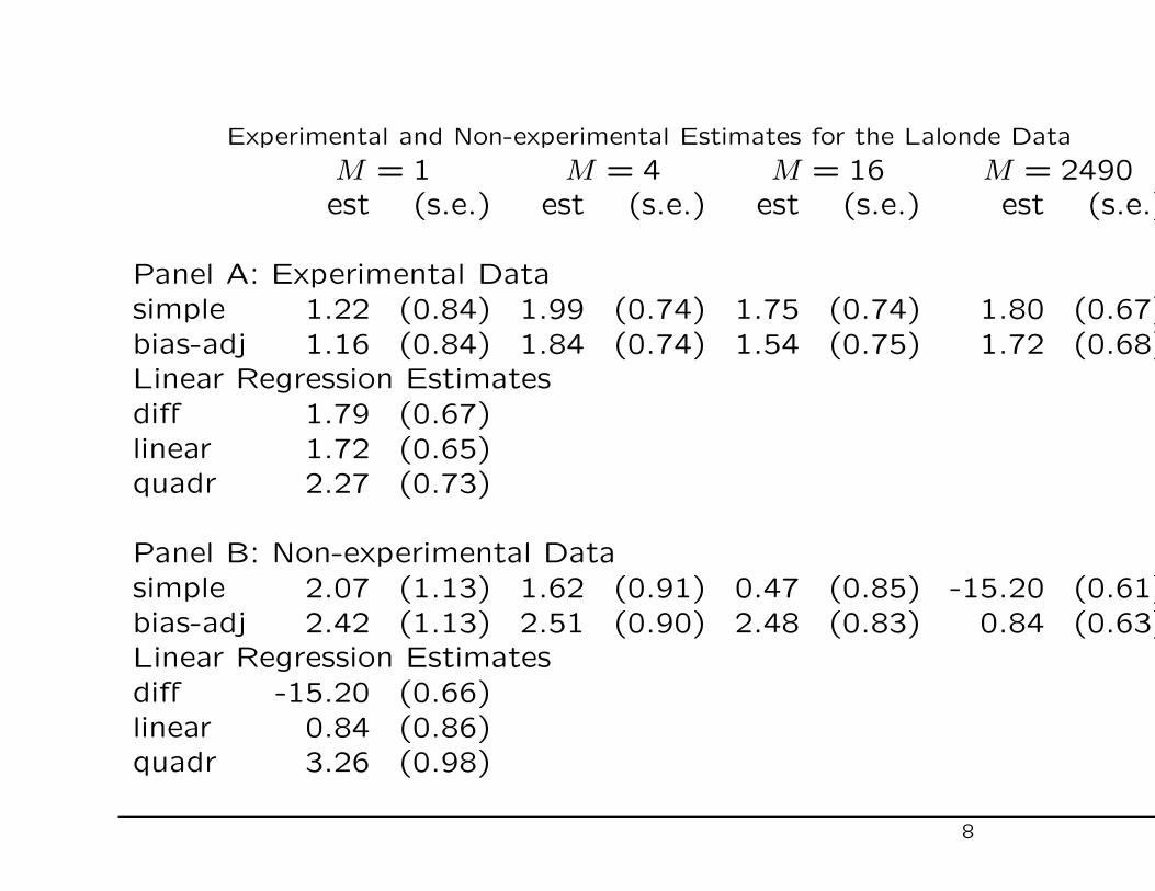
Experimental and Non-experimental Estimates for the Lalonde Data
M = 1 M = 4 M = 16 M = 2490est (s.e.) est (s.e.) est (s.e.) est (s.e.)
Panel A: Experimental Datasimple 1.22 (0.84) 1.99 (0.74) 1.75 (0.74) 1.80 (0.67)bias-adj 1.16 (0.84) 1.84 (0.74) 1.54 (0.75) 1.72 (0.68)Linear Regression Estimatesdiff 1.79 (0.67)linear 1.72 (0.65)quadr 2.27 (0.73)
Panel B: Non-experimental Datasimple 2.07 (1.13) 1.62 (0.91) 0.47 (0.85) -15.20 (0.61)bias-adj 2.42 (1.13) 2.51 (0.90) 2.48 (0.83) 0.84 (0.63)Linear Regression Estimatesdiff -15.20 (0.66)linear 0.84 (0.86)quadr 3.26 (0.98)
8
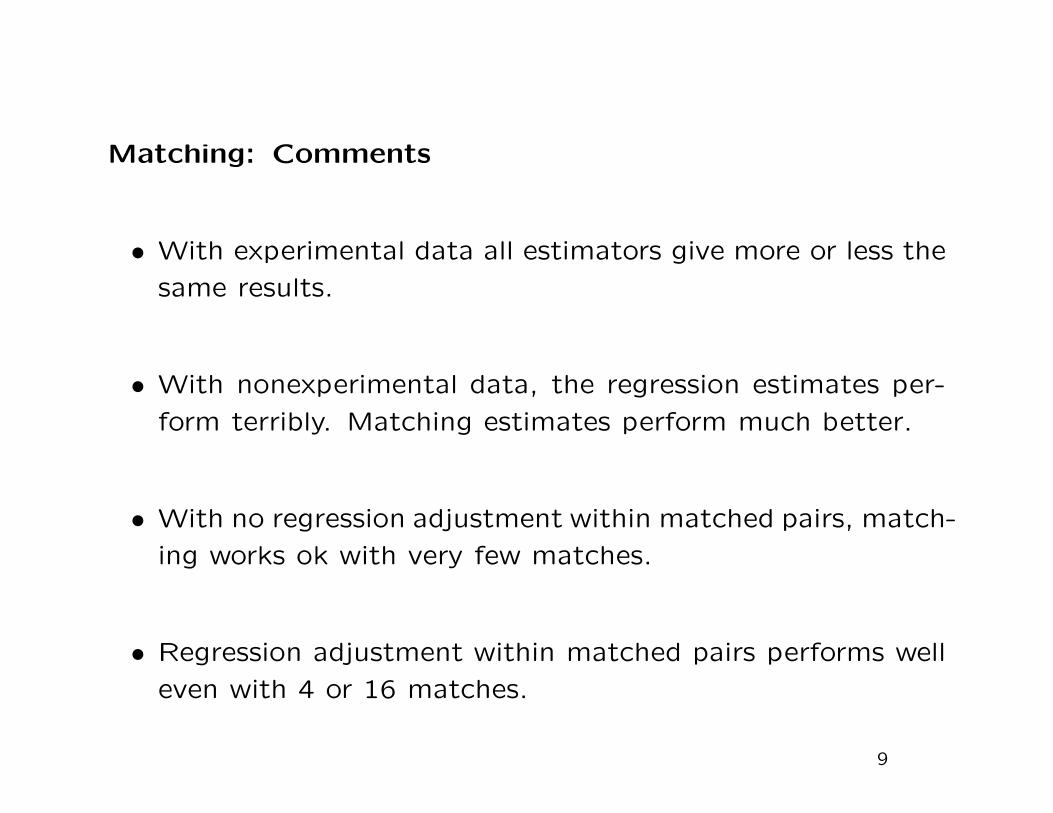
Matching: Comments
• With experimental data all estimators give more or less the
same results.
• With nonexperimental data, the regression estimates per-
form terribly. Matching estimates perform much better.
• With no regression adjustment within matched pairs, match-
ing works ok with very few matches.
• Regression adjustment within matched pairs performs well
even with 4 or 16 matches.
9
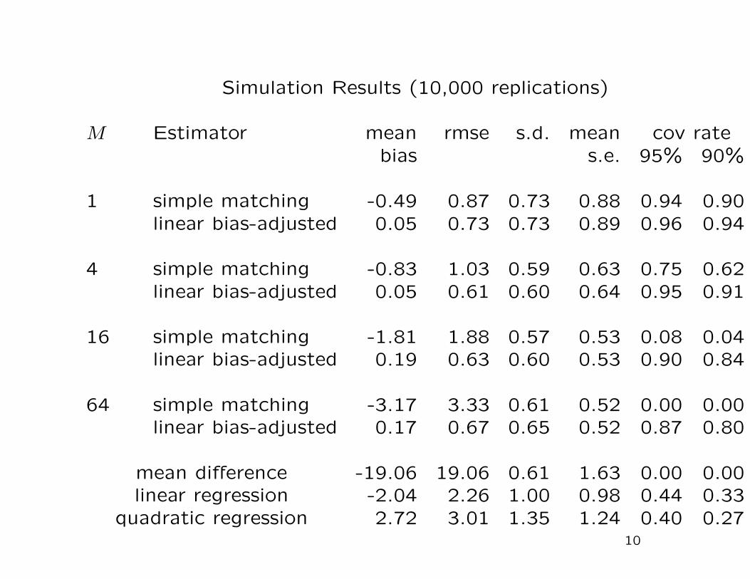
Simulation Results (10,000 replications)
M Estimator mean rmse s.d. mean cov ratebias s.e. 95% 90%
1 simple matching -0.49 0.87 0.73 0.88 0.94 0.90linear bias-adjusted 0.05 0.73 0.73 0.89 0.96 0.94
4 simple matching -0.83 1.03 0.59 0.63 0.75 0.62linear bias-adjusted 0.05 0.61 0.60 0.64 0.95 0.91
16 simple matching -1.81 1.88 0.57 0.53 0.08 0.04linear bias-adjusted 0.19 0.63 0.60 0.53 0.90 0.84
64 simple matching -3.17 3.33 0.61 0.52 0.00 0.00linear bias-adjusted 0.17 0.67 0.65 0.52 0.87 0.80
mean difference -19.06 19.06 0.61 1.63 0.00 0.00linear regression -2.04 2.26 1.00 0.98 0.44 0.33
quadratic regression 2.72 3.01 1.35 1.24 0.40 0.2710
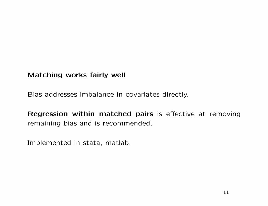
Matching works fairly well
Bias addresses imbalance in covariates directly.
Regression within matched pairs is effective at removing
remaining bias and is recommended.
Implemented in stata, matlab.
11
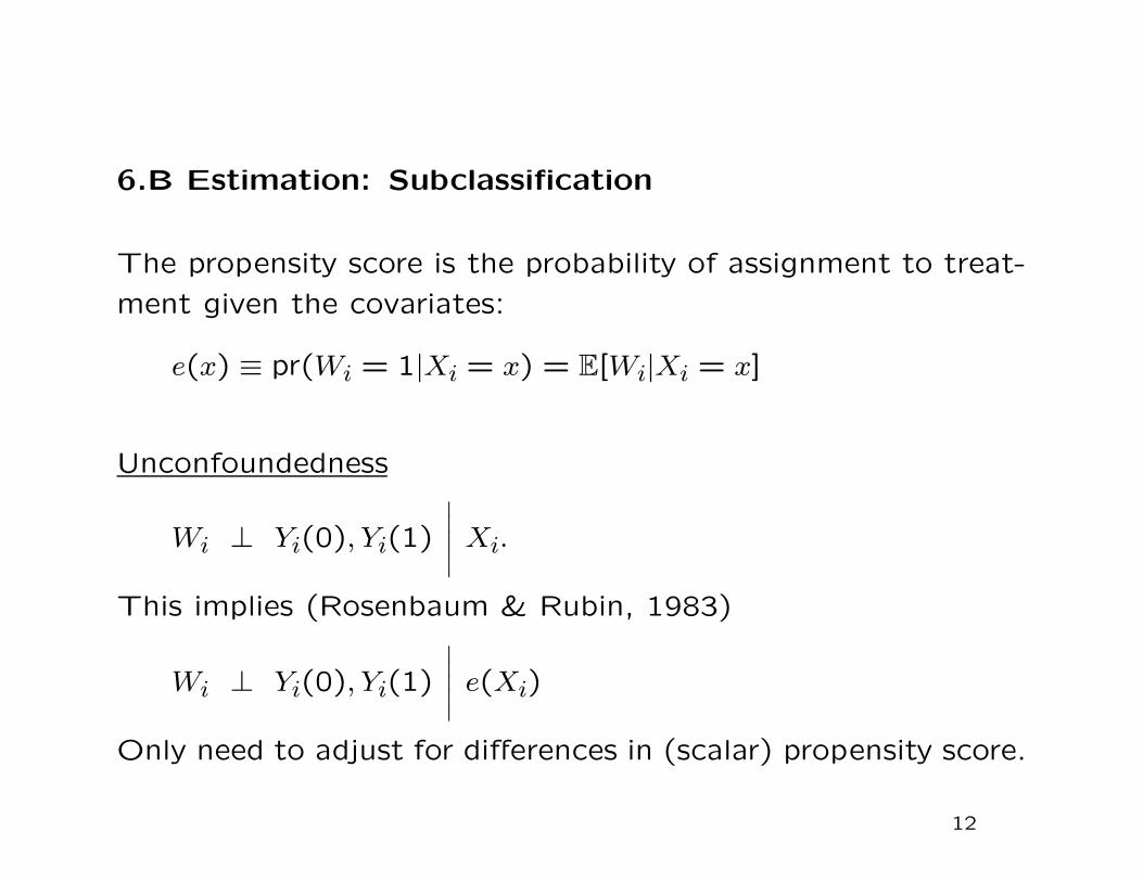
6.B Estimation: Subclassification
The propensity score is the probability of assignment to treat-
ment given the covariates:
e(x) ≡ pr(Wi = 1|Xi = x) = E[Wi|Xi = x]
Unconfoundedness
Wi ⊥ Yi(0), Yi(1)
∣∣∣∣∣ Xi.
This implies (Rosenbaum & Rubin, 1983)
Wi ⊥ Yi(0), Yi(1)
∣∣∣∣∣ e(Xi)
Only need to adjust for differences in (scalar) propensity score.
12

Implementation Using the Propensity Score
• Regression (compare to regression estimator with all covari-
ates)
Not recommended: not efficient (Hahn, 1998), functional
form is difficult to justify.
• Weighting on the Propensity Score
Exploit idea that
E
[Wi · Yi
e(Xi)
]
= E[Yi(1)] E
[(1 − Wi) · Yi
1 − e(Xi)
]
= E[Yi(0)]
Not recommended: sensitive to parametric form of propensity
score.
13
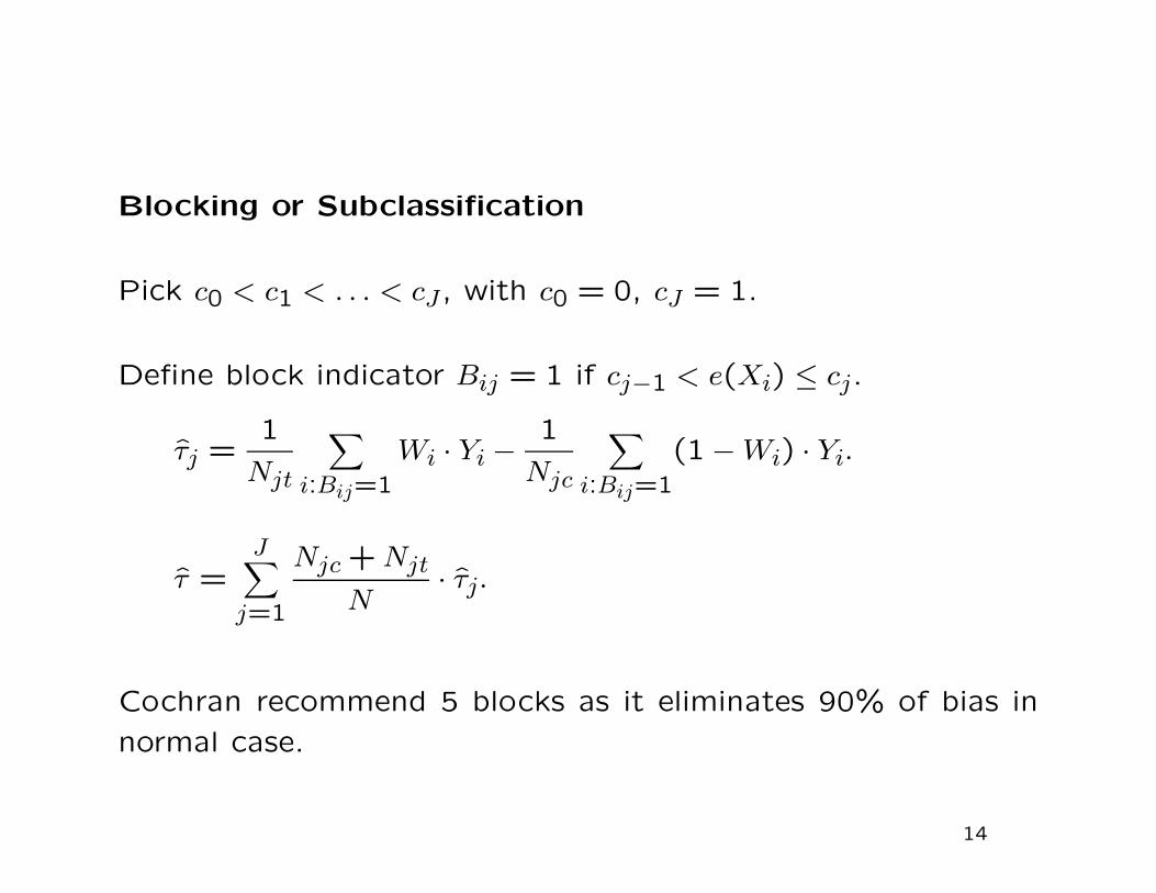
Blocking or Subclassification
Pick c0 < c1 < . . . < cJ , with c0 = 0, cJ = 1.
Define block indicator Bij = 1 if cj−1 < e(Xi) ≤ cj.
τj =1
Njt
∑
i:Bij=1
Wi · Yi −1
Njc
∑
i:Bij=1
(1 − Wi) · Yi.
τ =J∑
j=1
Njc + Njt
N· τj.
Cochran recommend 5 blocks as it eliminates 90% of bias in
normal case.
14

Lottery Data: Normalized Diffs in Covariates after SubclassificationFull Selected 2 Subclasses 5 Subclasses
Year Won -0.27 -0.06 0.03 -0.07Tickets Bought 0.90 0.51 -0.18 -0.07Age -0.47 -0.08 0.02 -0.04Male -0.19 -0.11 0.10 0.14Years of Schooling -0.70 -0.47 0.19 0.10Working Then 0.08 0.03 -0.03 -0.02Earnings Year -6 -0.27 -0.19 0.10 0.03...Earnings Year -1 -0.23 -0.19 0.02 -0.00Pos Earnings Year -6 0.03 -0.00 0.08 0.08...Pos Earnings Year -1 0.10 -0.01 0.04 0.07
15
Optimal Subclassification
Subclass Min P-score Max P-score # Controls # Treated
1 0.03 0.24 67 132 0.24 0.32 32 83 0.32 0.44 24 174 0.44 0.69 34 465 0.69 0.99 15 66
16
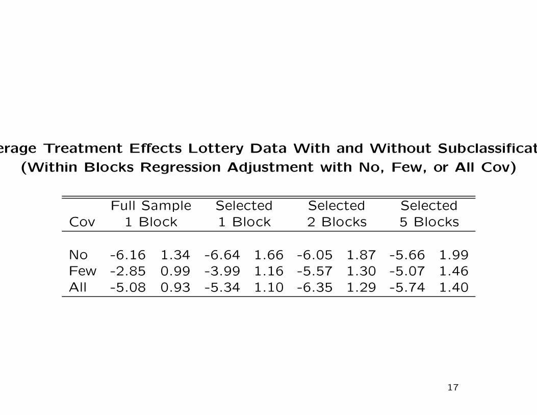
Average Treatment Effects Lottery Data With and Without Subclassification
(Within Blocks Regression Adjustment with No, Few, or All Cov)
Full Sample Selected Selected SelectedCov 1 Block 1 Block 2 Blocks 5 Blocks
No -6.16 1.34 -6.64 1.66 -6.05 1.87 -5.66 1.99Few -2.85 0.99 -3.99 1.16 -5.57 1.30 -5.07 1.46All -5.08 0.93 -5.34 1.10 -6.35 1.29 -5.74 1.40
17
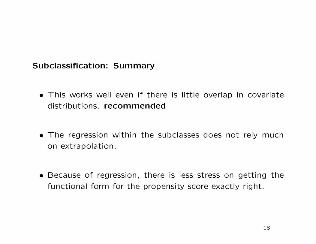
Subclassification: Summary
• This works well even if there is little overlap in covariate
distributions. recommended
• The regression within the subclasses does not rely much
on extrapolation.
• Because of regression, there is less stress on getting the
functional form for the propensity score exactly right.
18

7. Assessing Unconfoundedness
Main question:
• what can we say about the plausibility of unconfounded-
ness?
• Recall, unconfoundedness is not testable.
19

Assessing Unconfoundedness: Two Approaches
Both approaches estimate zero effects:
• Estimate effect of treatment on pseudo outcome
• Estimate effectof pseudo treatment on outcome
20
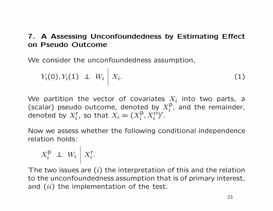
7. A Assessing Unconfoundedness by Estimating Effecton Pseudo Outcome
We consider the unconfoundedness assumption,
Yi(0), Yi(1) ⊥⊥ Wi
∣∣∣∣∣ Xi. (1)
We partition the vector of covariates Xi into two parts, a(scalar) pseudo outcome, denoted by Xp
i , and the remainder,denoted by Xr
i , so that Xi = (Xpi , Xr′
i )′.
Now we assess whether the following conditional independencerelation holds:
Xpi ⊥⊥ Wi
∣∣∣∣∣ Xri .
The two issues are (i) the interpretation of this and the relationto the unconfoundedness assumption that is of primary interest,and (ii) the implementation of the test.
21

The first issue concerns the link between the conditional inde-
pendence relation and unconfoundedness . This link is indirect,
as unconfoundedness cannot be tested directly.
First consider a related condition:
Yi(0), Yi(1) ⊥⊥ Wi
∣∣∣∣∣ Xri .
If this modified unconfoundedness condition were to hold, one
could use the adjustment methods using only the subset of
covariates Xri . In practice this is a stronger condition than the
original unconfoundedness condition.
The modified unconfoundedness condition is not testable. We
use the pseudo outcome Xpi as a proxy variable Yi(0), and test
Xpi ⊥⊥ Wi
∣∣∣∣∣ Xri .
22
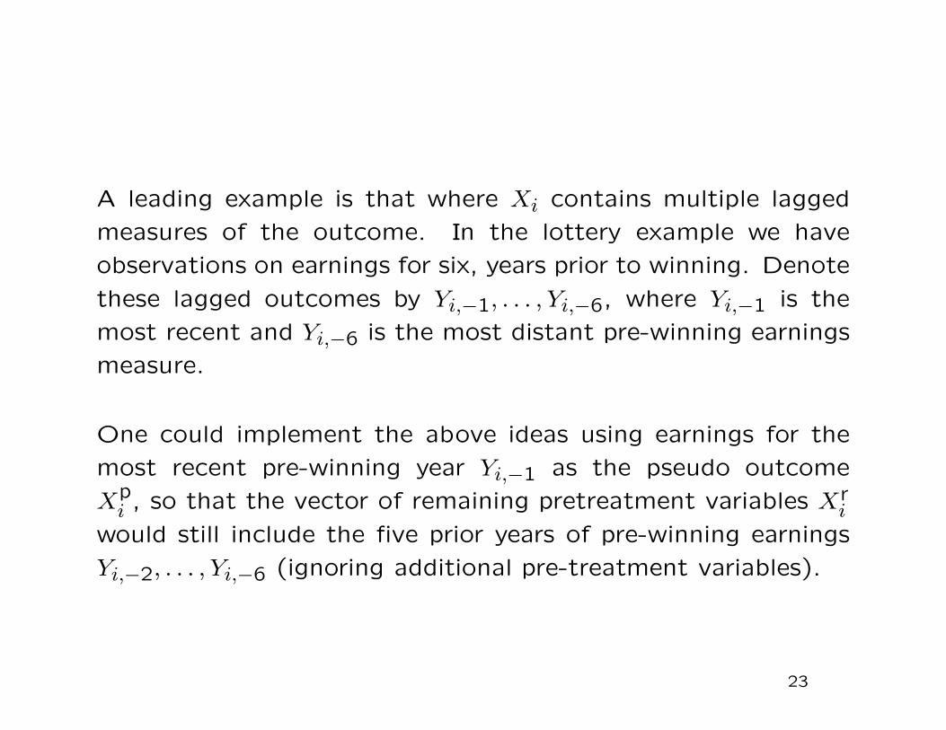
A leading example is that where Xi contains multiple lagged
measures of the outcome. In the lottery example we have
observations on earnings for six, years prior to winning. Denote
these lagged outcomes by Yi,−1, . . . , Yi,−6, where Yi,−1 is the
most recent and Yi,−6 is the most distant pre-winning earnings
measure.
One could implement the above ideas using earnings for the
most recent pre-winning year Yi,−1 as the pseudo outcome
Xpi , so that the vector of remaining pretreatment variables Xr
i
would still include the five prior years of pre-winning earnings
Yi,−2, . . . , Yi,−6 (ignoring additional pre-treatment variables).
23

Now we turn to the second issue, the implementation. One
approach to testing the conditional independence assumption
is to estimate the average difference in Xpi by treatment status,
after adjusting for differences in Xri .
This is exactly the same problem as estimating the average
effect of the treatment, using Xpi as the pseudo outcome and
Xri as the vector of pretreatment variables. We can do this
using any of the methods discussed so far.
24
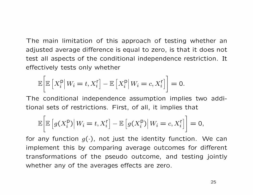
The main limitation of this approach of testing whether an
adjusted average difference is equal to zero, is that it does not
test all aspects of the conditional independence restriction. It
effectively tests only whether
E
[
E
[Xp
i
∣∣∣Wi = t,Xri
]− E
[Xp
i
∣∣∣Wi = c, Xri
]]
= 0.
The conditional independence assumption implies two addi-
tional sets of restrictions. First, of all, it implies that
E
[
E
[g(Xp
i )∣∣∣Wi = t,Xr
i
]− E
[g(Xp
i )∣∣∣Wi = c, Xr
i
]]
= 0,
for any function g(·), not just the identity function. We can
implement this by comparing average outcomes for different
transformations of the pseudo outcome, and testing jointly
whether any of the averages effects are zero.
25
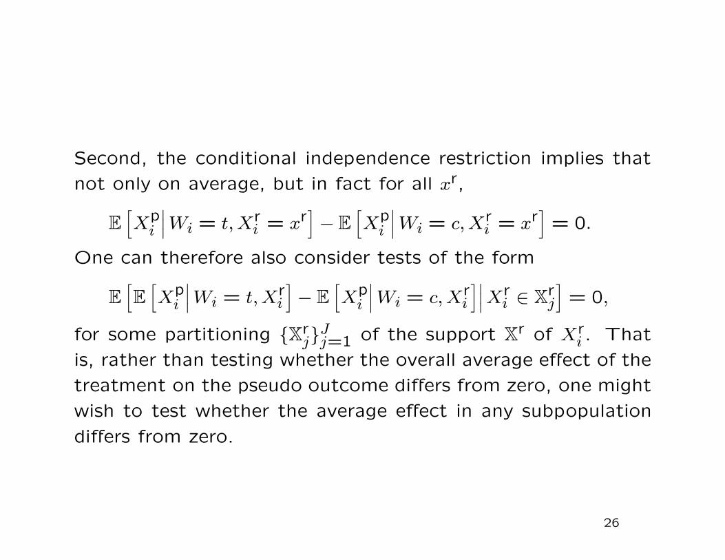
Second, the conditional independence restriction implies that
not only on average, but in fact for all xr,
E
[Xp
i
∣∣∣Wi = t, Xri = xr
]− E
[Xp
i
∣∣∣Wi = c, Xri = xr
]= 0.
One can therefore also consider tests of the form
E
[E
[Xp
i
∣∣∣Wi = t, Xri
]− E
[Xp
i
∣∣∣Wi = c, Xri
]∣∣∣Xri ∈ X
rj
]= 0,
for some partitioning Xrj
Jj=1 of the support X
r of Xri . That
is, rather than testing whether the overall average effect of the
treatment on the pseudo outcome differs from zero, one might
wish to test whether the average effect in any subpopulation
differs from zero.
26
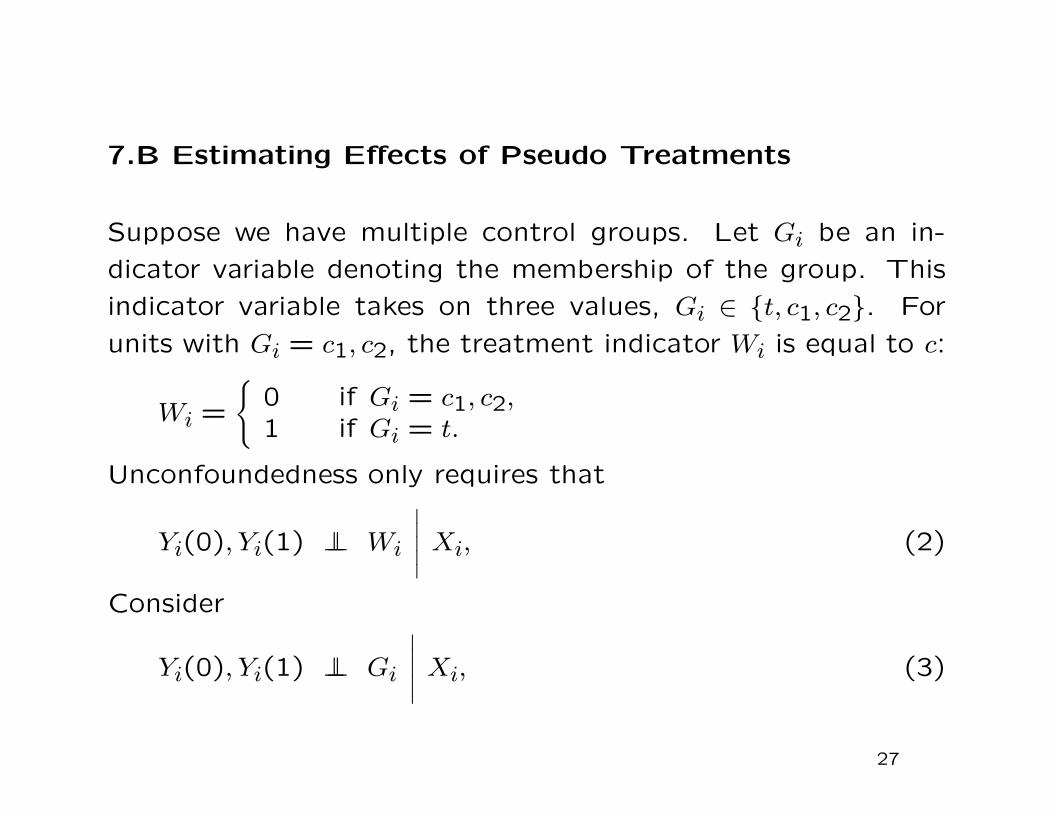
7.B Estimating Effects of Pseudo Treatments
Suppose we have multiple control groups. Let Gi be an in-
dicator variable denoting the membership of the group. This
indicator variable takes on three values, Gi ∈ t, c1, c2. For
units with Gi = c1, c2, the treatment indicator Wi is equal to c:
Wi =
0 if Gi = c1, c2,1 if Gi = t.
Unconfoundedness only requires that
Yi(0), Yi(1) ⊥⊥ Wi
∣∣∣∣∣ Xi, (2)
Consider
Yi(0), Yi(1) ⊥⊥ Gi
∣∣∣∣∣ Xi, (3)
27
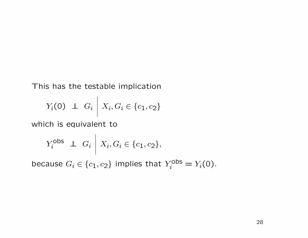
This has the testable implication
Yi(0) ⊥⊥ Gi
∣∣∣∣∣ Xi, Gi ∈ c1, c2
which is equivalent to
Y obsi ⊥⊥ Gi
∣∣∣∣∣ Xi, Gi ∈ c1, c2,
because Gi ∈ c1, c2 implies that Y obsi = Yi(0).
28
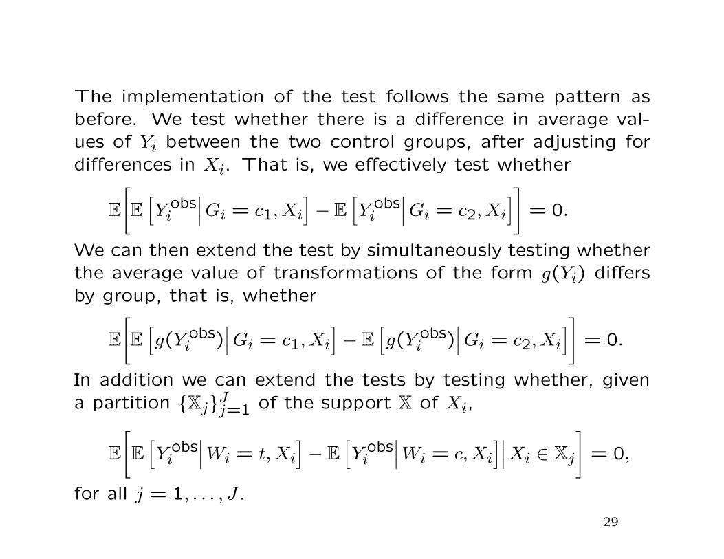
The implementation of the test follows the same pattern as
before. We test whether there is a difference in average val-
ues of Yi between the two control groups, after adjusting for
differences in Xi. That is, we effectively test whether
E
[
E
[Y obs
i
∣∣∣Gi = c1, Xi
]− E
[Y obs
i
∣∣∣Gi = c2, Xi
]]
= 0.
We can then extend the test by simultaneously testing whether
the average value of transformations of the form g(Yi) differs
by group, that is, whether
E
[
E
[g(Y obs
i )∣∣∣Gi = c1, Xi
]− E
[g(Y obs
i )∣∣∣Gi = c2, Xi
]]
= 0.
In addition we can extend the tests by testing whether, given
a partition XjJj=1 of the support X of Xi,
E
[
E
[Y obs
i
∣∣∣Wi = t, Xi
]− E
[Y obs
i
∣∣∣Wi = c, Xi
]∣∣∣Xi ∈ Xj
]
= 0,
for all j = 1, . . . , J.
29
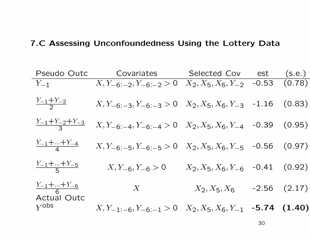
7.C Assessing Unconfoundedness Using the Lottery Data
Pseudo Outc Covariates Selected Cov est (s.e.)
Y−1 X, Y−6:−2, Y−6:−2 > 0 X2, X5, X6, Y−2 -0.53 (0.78)
Y−1+Y−22 X, Y−6:−3, Y−6:−3 > 0 X2, X5, X6, Y−3 -1.16 (0.83)
Y−1+Y−2+Y−33 X, Y−6:−4, Y−6:−4 > 0 X2, X5, X6, Y−4 -0.39 (0.95)
Y−1+...+Y−44 X, Y−6:−5, Y−6:−5 > 0 X2, X5, X6, Y−5 -0.56 (0.97)
Y−1+...+Y−55 X, Y−6, Y−6 > 0 X2, X5, X6, Y−6 -0.41 (0.92)
Y−1+...+Y−66 X X2, X5, X6 -2.56 (2.17)
Actual Outc
Y obs X, Y−1:−6, Y−6:−1 > 0 X2, X5, X6, Y−1 -5.74 (1.40)
30

Estimates of Average Treatment Effect
on Transformations of Pseudo Outcome for Subpopulations
Pseudo Subpopulation est (s.e.)Outcome
1Y−1 = 0 Y−2 = 0 -0.07 (0.78)1Y−1 = 0 Y−2 > 0 0.02 (0.02)Y−1 Y−2 = 0 -0.31 (0.30)Y−1 Y−2 > 0 0.05 (0.06)
statistic p-valueCombined Statistic(chi-squared, dof 4) 2.20 0.135
31
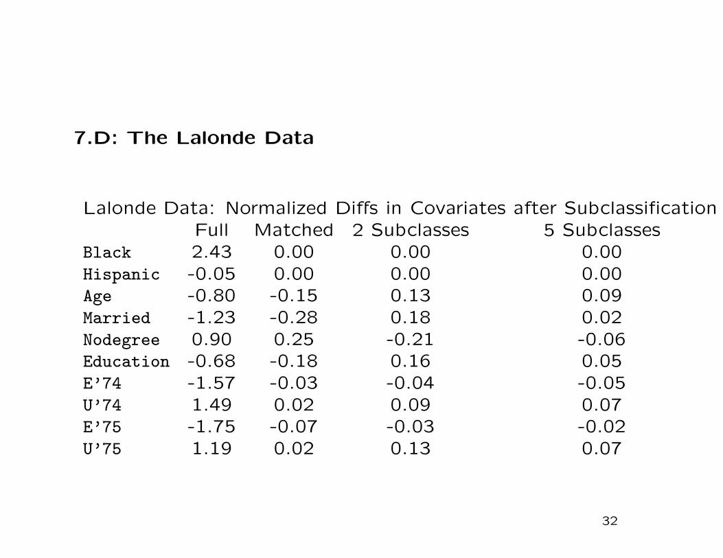
7.D: The Lalonde Data
Lalonde Data: Normalized Diffs in Covariates after SubclassificationFull Matched 2 Subclasses 5 Subclasses
Black 2.43 0.00 0.00 0.00Hispanic -0.05 0.00 0.00 0.00Age -0.80 -0.15 0.13 0.09Married -1.23 -0.28 0.18 0.02Nodegree 0.90 0.25 -0.21 -0.06Education -0.68 -0.18 0.16 0.05E’74 -1.57 -0.03 -0.04 -0.05U’74 1.49 0.02 0.09 0.07E’75 -1.75 -0.07 -0.03 -0.02U’75 1.19 0.02 0.13 0.07
32

Next let us look at the estimates for effect on 1978 earnings.
We use the matched sample and use subclassification to re-
move additional bias.
Full Sample Matched Matched MatchedCov 1 Block 1 Block 2 Blocks 4 Blocks
No -8.50 0.58 1.72 0.74 1.81 0.75 1.86 0.76Few 0.69 0.59 1.81 0.73 1.80 0.73 1.99 0.75All 1.07 0.55 1.97 0.66 1.90 0.67 2.06 0.66
33

Covariate still make some difference, but reasonably robust.
With all covariates included the estimate is close to experimen-
tal one, but would we have known that?
With only the trainee and CPS comparison data would we have
concluded that the evaluation was succesful?
34
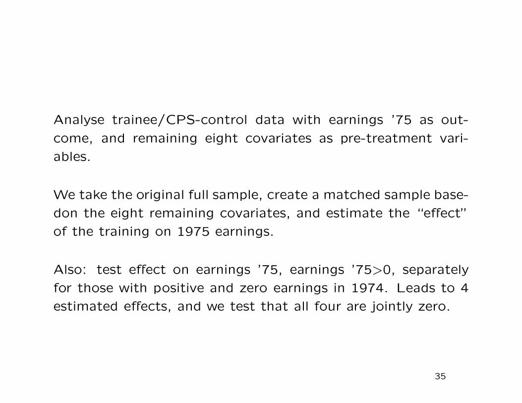
Analyse trainee/CPS-control data with earnings ’75 as out-
come, and remaining eight covariates as pre-treatment vari-
ables.
We take the original full sample, create a matched sample base-
don the eight remaining covariates, and estimate the “effect”
of the training on 1975 earnings.
Also: test effect on earnings ’75, earnings ’75>0, separately
for those with positive and zero earnings in 1974. Leads to 4
estimated effects, and we test that all four are jointly zero.
35
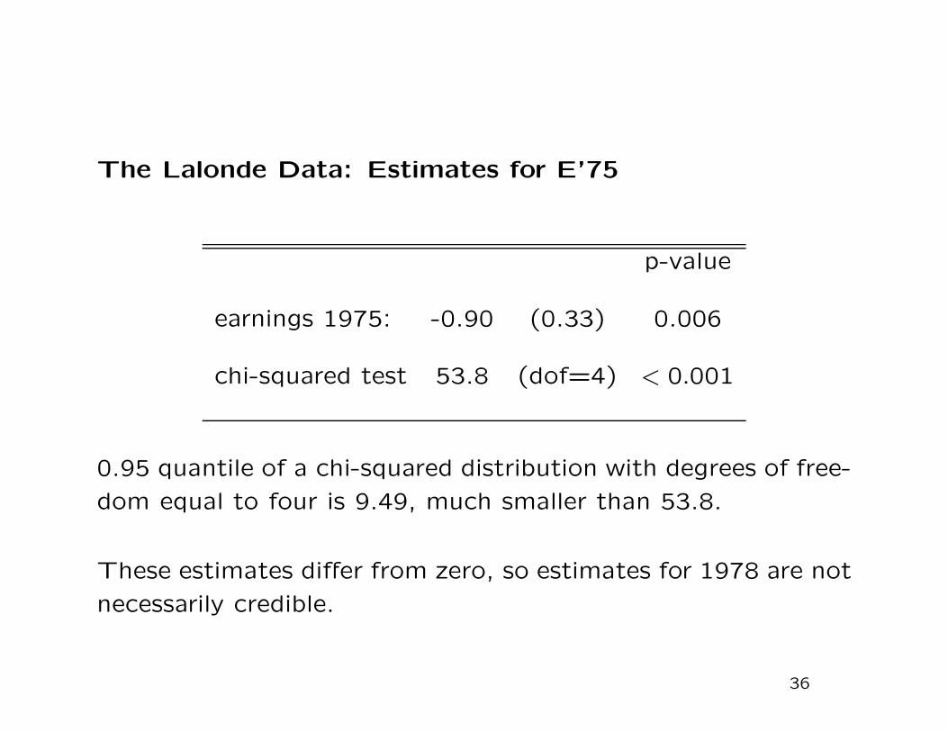
The Lalonde Data: Estimates for E’75
p-value
earnings 1975: -0.90 (0.33) 0.006
chi-squared test 53.8 (dof=4) < 0.001
0.95 quantile of a chi-squared distribution with degrees of free-
dom equal to four is 9.49, much smaller than 53.8.
These estimates differ from zero, so estimates for 1978 are not
necessarily credible.
36

In the Lalonde case, had we done this analysis first, we would
not necessarily have even estimated the effect for 1978 earn-
ings: the initial analysis suggests that the estimates would not
necessarily be credible.
37

7.E Assessing Unconfoundedness: Summary
Whenever possible, assess the plausibility of unconfoundedness.
Having good covariates available is important here.
Analysis may suggest that results are not credible. They dont
point in direction of alternative analysis, only suggest that pro-
ceeding under the assumption of unconfoundedness is not rea-
sonable.
38

• for the lottery data we obtain credible and precise estimates,
robust to small changes in the specification and with uncon-
foundedness plausible.
• for the lalonde data the results are more mixed. the estimates
are robust to changes in the specification, but the assessments
of unconfoundedness raises doubts.
39

Econometrics of Cross Section and Panel DataLecture 3: Linear Panel Data Models I
Jeff WooldridgeMichigan State University
cemmap/PEPA, June 2014
1. Introduction and Summary2. The Basic Model and Assumptions3. The Standard Estimators4. Comparing RE and FE5. Comparing FE and FD
1
1. Introduction and Summary∙Microeconometric setting: Access to a large cross sectionand short time series.∙ Random sampling in the cross section.∙ Important to think through the assumptions that implyconsistency for the different estimators. What is the sourceof bias?∙ Distinguish between “ideal” assumptions and thosesufficient for consistent estimation.
2
∙ Inference robust to general serial correlation andheteroskedasticity should be used.∙When using specification tests (Hausman test), make testsas robust as inference on the coefficients.
3
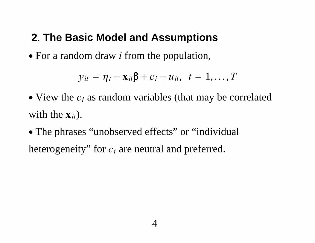
2. The Basic Model and Assumptions∙ For a random draw i from the population,
yit t xit ci uit, t 1, . . . ,T
∙ View the ci as random variables (that may be correlatedwith the xit).∙ The phrases “unobserved effects” or “individualheterogeneity” for ci are neutral and preferred.
4

yit t xit ci uit, t 1, . . . ,T
∙ The uit : t 1, . . . ,T are the idiosyncratic errors.∙ The composite error at time t is
vit ci uit
∙ Except by fluke vit : t 1, . . . ,T is serially correlated,and could be heteroskedastic.
5
yit t xit ci uit, t 1, . . . ,T
∙ xit is a 1 K row vector; it can contain variables thatchange across i only, or across i and t.∙With a short panel, the time period intercepts, t, are
usually treated as parameters that can be estimated.∙ Separate period intercepts are handled easily with timedummies.
6
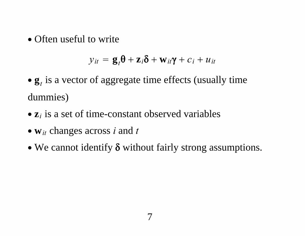
∙ Often useful to write
yit gt zi wit ci uit
∙ gt is a vector of aggregate time effects (usually time
dummies)∙ zi is a set of time-constant observed variables∙ wit changes across i and t∙We cannot identify without fairly strong assumptions.
7
Assumptions about Covariates and IdiosyncraticErrors
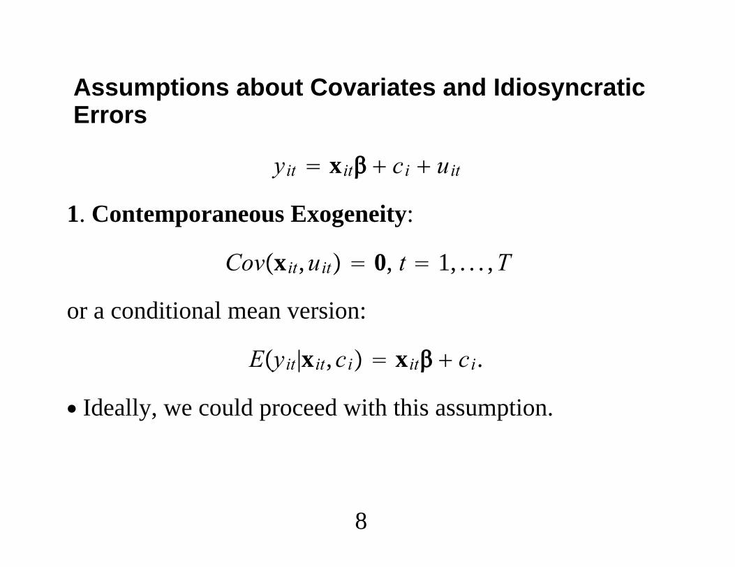
yit xit ci uit
1. Contemporaneous Exogeneity:
Covxit,uit 0, t 1, . . . ,T
or a conditional mean version:
Eyit|xit,ci xit ci.
∙ Ideally, we could proceed with this assumption.
8
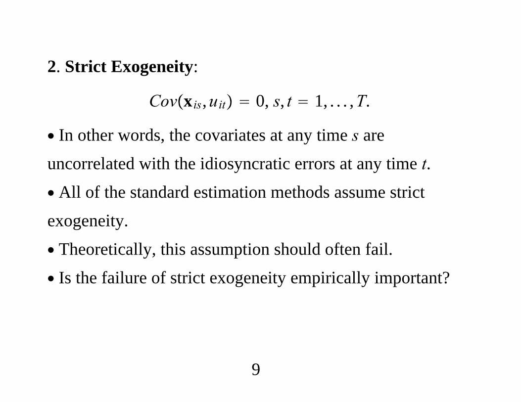
2. Strict Exogeneity:
Covxis,uit 0, s, t 1, . . . ,T.
∙ In other words, the covariates at any time s areuncorrelated with the idiosyncratic errors at any time t.∙ All of the standard estimation methods assume strictexogeneity.∙ Theoretically, this assumption should often fail.∙ Is the failure of strict exogeneity empirically important?
9
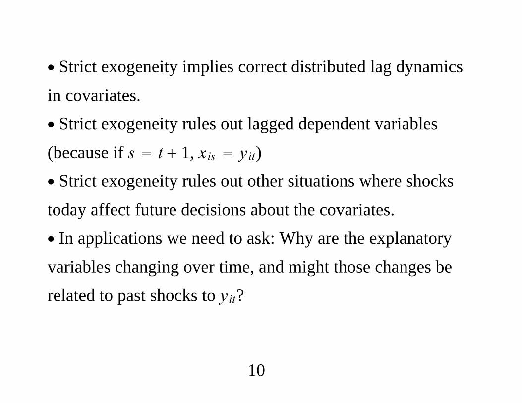
∙ Strict exogeneity implies correct distributed lag dynamicsin covariates.∙ Strict exogeneity rules out lagged dependent variables(because if s t 1, xis yit)∙ Strict exogeneity rules out other situations where shockstoday affect future decisions about the covariates.∙ In applications we need to ask: Why are the explanatoryvariables changing over time, and might those changes berelated to past shocks to yit?
10

∙ Example: If a worker changes his union status, is hereacting to past shocks to earnings?∙ Example: Do shocks to air fares feed back into futurechanges in route concentration?∙ Example: Might a principal assign students to classroomsbased on past shocks to academic performance?
11

3. Sequential Exogeneity:
Covxis,uit 0, s ≤ t
∙ This assumption can hold with lagged dependent variables,but it does require correct dynamic specification.∙ Key: Sequential exogeneity is silent on feedback. It allowsxi,t1 to be correlated with uit.
12

Assumptions about Covariates and UnobservedEffect
yit xit ci uit
1. “Random effects” means
Covxit,ci 0, t 1, . . . ,T.
2. “Fixed effects” means that no restrictions are placed onthe relationship between ci and xit.3. “Correlated random effects” (CRE): We model therelationship between ci and xit.
13

3. The Standard Estimators∙ Best to think of there being one model, the unobservedeffects model
yit xit ci uit, i 1, . . . ,T.
∙ There are several possible estimators of .
∙ “OLS Model”?
14

3.1. Pooled OLS∙ Pool the observations and apply OLS:
yit xit vitvit ci uit
∙ Consistency (fixed T, N → ) of POLS ensured by
Covxit,ci 0Covxit,uit 0, t 1, . . . ,T.
15
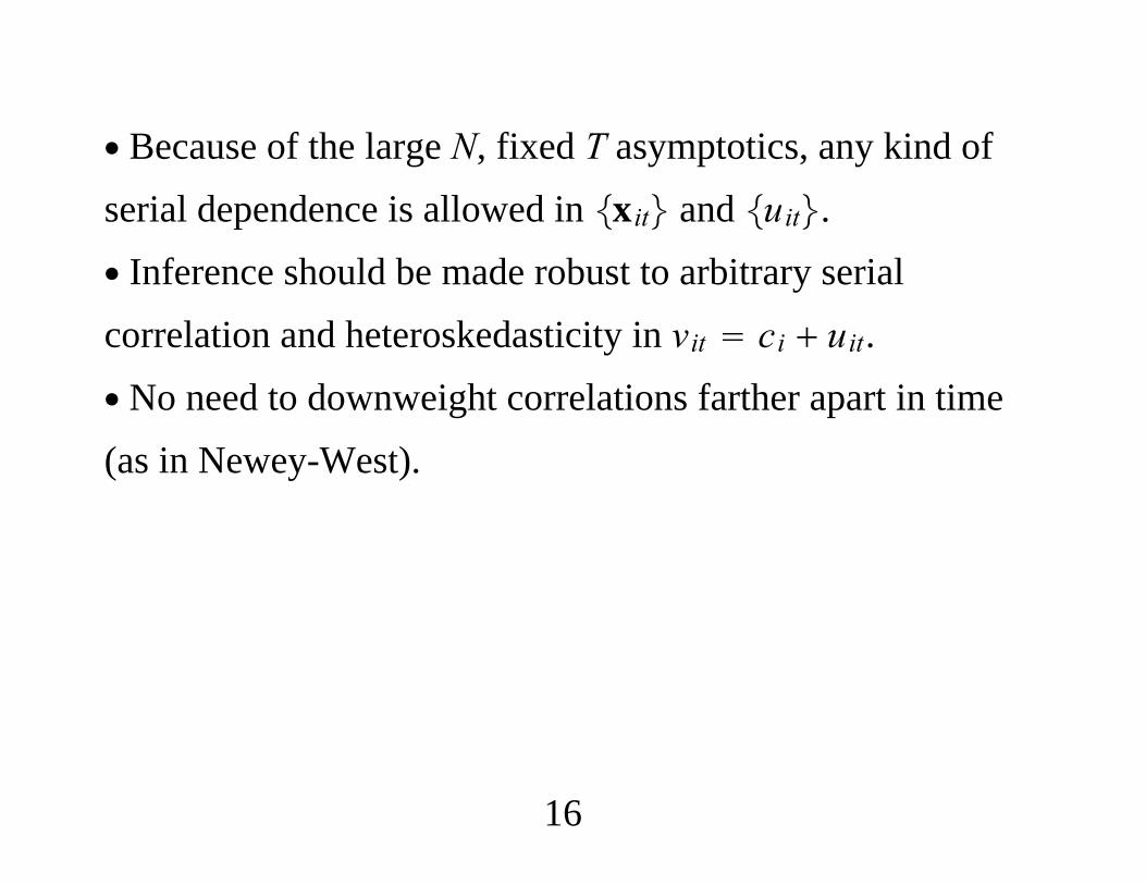
∙ Because of the large N, fixed T asymptotics, any kind ofserial dependence is allowed in xit and uit.∙ Inference should be made robust to arbitrary serialcorrelation and heteroskedasticity in vit ci uit.∙ No need to downweight correlations farther apart in time(as in Newey-West).
16
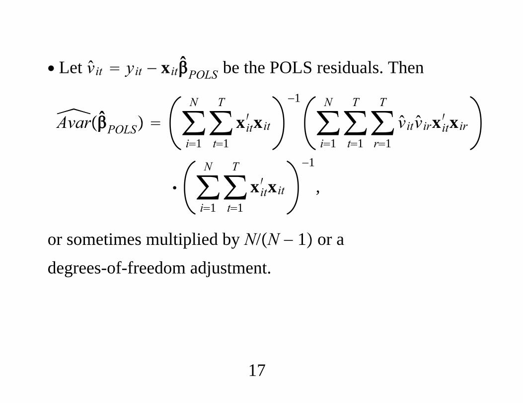
∙ Let vit yit − xitPOLS be the POLS residuals. Then
AvarPOLS ∑i1
N
∑t1
T
xit′ xit−1
∑i1
N
∑t1
T
∑r1
T
vitvirxit′ xir
∑i1
N
∑t1
T
xit′ xit−1
,
or sometimes multiplied by N/N − 1 or adegrees-of-freedom adjustment.
17

∙ Can include aggregate time effects, variables that changeonly across units, and variables that change across i and t.∙With good controls – say, industry dummies when we havefirm-level data or state dummies with county-level data – wemight find Covxit,ci 0 plausible.∙ (Quasi-)randomization of an intervention?∙ Dynamic OLS, which includes lagged yit, useful for“astructural” treatment effects estimation.
18

3.2. Random Effects Estimation∙ RE assumes
Covxit,ci 0Covxis,uit 0, s, t 1, . . . ,T.
∙ Letting xi xi1,xi2, . . . ,xiT, vit ci uit is uncorrelatedwith xi (not just xit).∙We can apply generalized least squares methods.
19
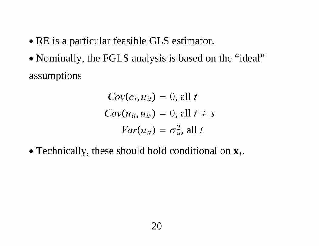
∙ RE is a particular feasible GLS estimator.∙ Nominally, the FGLS analysis is based on the “ideal”assumptions
Covci,uit 0, all tCovuit,uis 0, all t ≠ s
Varuit u2, all t
∙ Technically, these should hold conditional on xi.
20

Evivi′
c2 u2 c2 c2
c2 c2 u2
c2
c2 c2 c2 u2
∙ Depends on only two parameters, c2 Varci andu2 Varuit, rather than TT 1/2.
21
∙ Two ways that RE can fail to be true GLS: The unconditional variance-covariance matrix, Varvi,does not have the RE form. It could be any T T symmetric,positive definite matrix. Varvi|xi ≠ Varvi so there is “systemheteroskedasticity”: the conditional variances or covariancesdepend on xi.
22
∙ Important: RE is generally consistent provided
Covxit,vis 0, all t, s
and we rule out perfect collinearity in xit.∙ The true Varvi|xi can be of any form and not affectconsistency.
23
∙ RE is “quasi-” GLS when the RE variance structure doesnot hold.∙ RE still can be notably better than pooled OLS. (Keyinsight in Generalized Estimating Equations literature.)∙ Serial correlation in uit or heteroskedasticity in ci or uitmeans we should make inference fully robust.
24
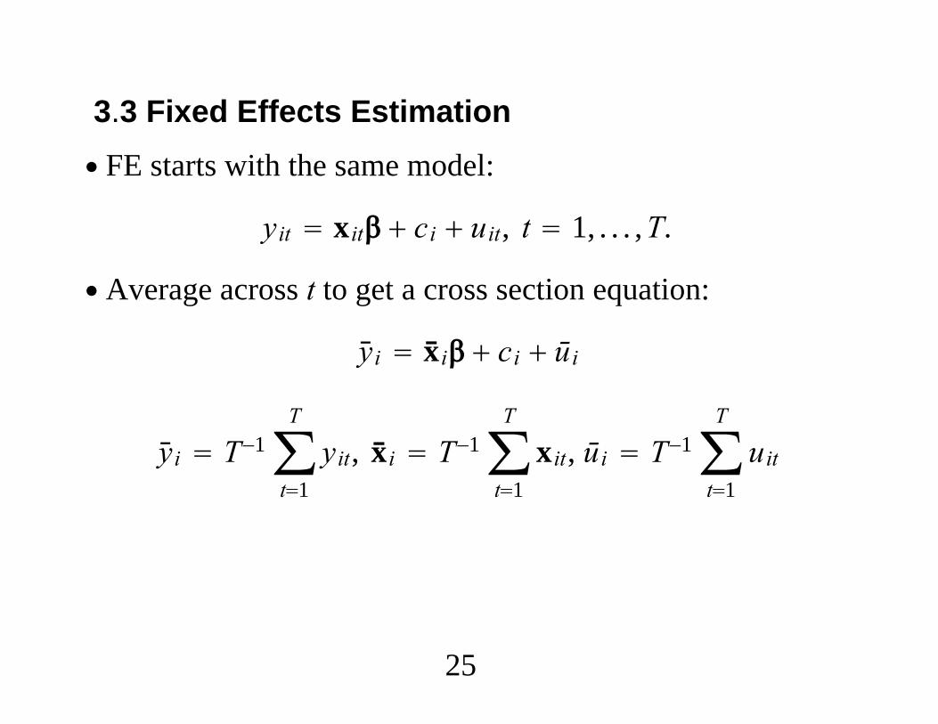
3.3 Fixed Effects Estimation∙ FE starts with the same model:
yit xit ci uit, t 1, . . . ,T.
∙ Average across t to get a cross section equation:
yi xi ci ūi
yi T−1∑t1
T
yit, xi T−1∑t1
T
xit, ūi T−1∑t1
T
uit
25
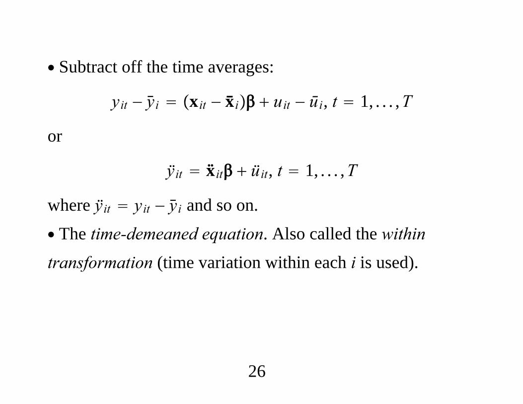
∙ Subtract off the time averages:
yit − yi xit − xi uit − ūi, t 1, . . . ,T
or
ÿit xit üit, t 1, . . . ,T
where ÿit yit − yi and so on.∙ The time-demeaned equation. Also called the withintransformation (time variation within each i is used).
26
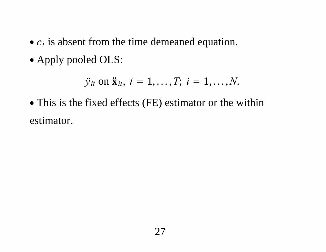
∙ ci is absent from the time demeaned equation.∙ Apply pooled OLS:
ÿit on xit, t 1, . . . ,T; i 1, . . . ,N.
∙ This is the fixed effects (FE) estimator or the withinestimator.
27

∙ Least restrictive exogeneity condition for consistency:
∑t1
T
Exit − xi′uit 0.
∙ Essentially, for t 1, . . . ,T,
Exit′ uit 0Exi′uit 0
∙ Relationship between ci and xit is unrestricted.
28
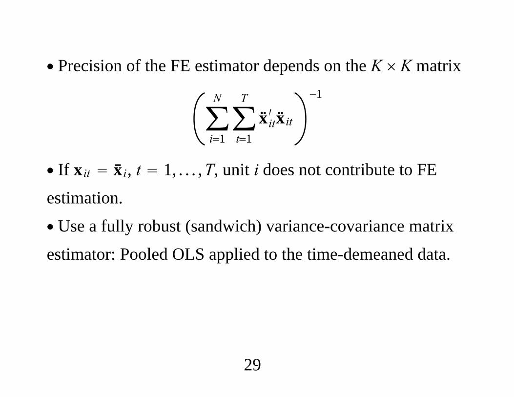
∙ Precision of the FE estimator depends on the K K matrix
∑i1
N
∑t1
T
xit′ xit−1
∙ If xit xi, t 1, . . . ,T, unit i does not contribute to FEestimation.∙ Use a fully robust (sandwich) variance-covariance matrixestimator: Pooled OLS applied to the time-demeaned data.
29
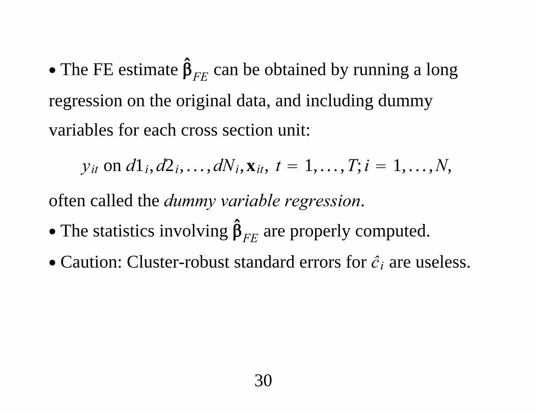
∙ The FE estimate FE can be obtained by running a long
regression on the original data, and including dummyvariables for each cross section unit:
yit on d1i,d2i, . . . ,dNi,xit, t 1, . . . ,T; i 1, . . . ,N,
often called the dummy variable regression.
∙ The statistics involving FE are properly computed.
∙ Caution: Cluster-robust standard errors for ĉi are useless.
30
Practical Hints1. Possible confusion concerning “fixed effects.” Suppose i is a firm. Then the phrase “firm fixed effect”corresponds to allowing ci in the model to be correlated withthe covariates. Instead, we can include in xit a set of industry dummyvariables and then account for the presence of the firmeffect, ci, in a random effects framework.
31
If there are many firms per industry, the industry “fixedeffects” can be precisly estimated. Including dummies for more aggregated levels and thenapplying RE is common when the covariates of interest varyby firm but not (much) by time.
32
2. For most applications, unless T is large, a full set oftime-period effects should be included.(i) Any aggregate time variables are automatically accountedfor.(ii) It guards against spuriously concluding that a policy didor did not have an effect.(iii) Using time dummies can reduce cross-sectionalcorrelation.
33
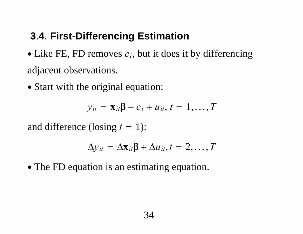
3.4. First-Differencing Estimation∙ Like FE, FD removes ci, but it does it by differencingadjacent observations.∙ Start with the original equation:
yit xit ci uit, t 1, . . . ,T
and difference (losing t 1):
Δyit Δxit Δuit, t 2, . . . ,T
∙ The FD equation is an estimating equation.
34
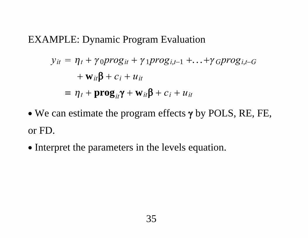
EXAMPLE: Dynamic Program Evaluation
yit t 0progit 1progi,t−1 . . .Gprogi,t−G wit ci uit
≡ t progit wit ci uit
∙We can estimate the program effects by POLS, RE, FE,
or FD.∙ Interpret the parameters in the levels equation.
35
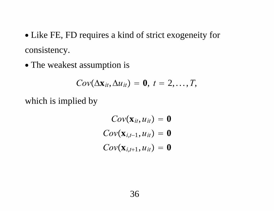
∙ Like FE, FD requires a kind of strict exogeneity forconsistency.∙ The weakest assumption is
CovΔxit,Δuit 0, t 2, . . . ,T,
which is implied by
Covxit,uit 0Covxi,t−1,uit 0Covxi,t1,uit 0
36
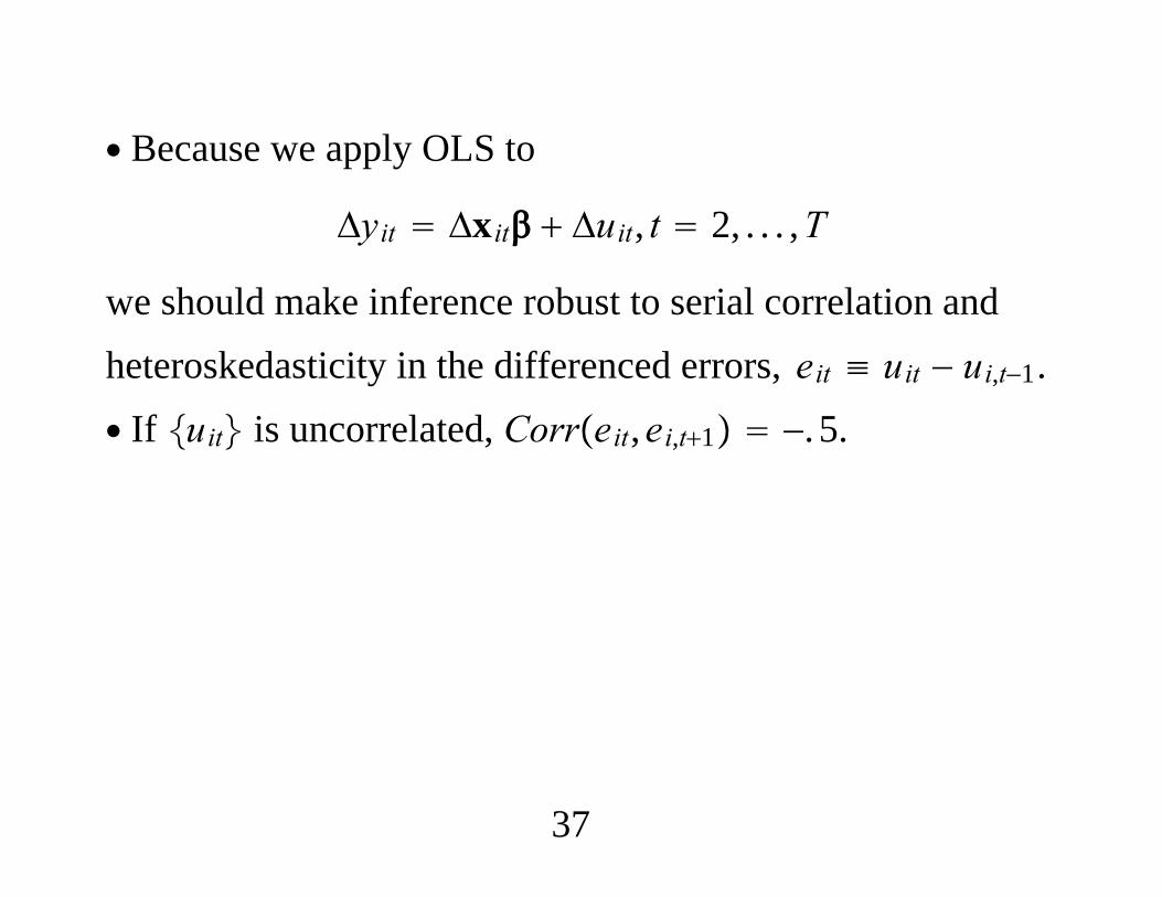
∙ Because we apply OLS to
Δyit Δxit Δuit, t 2, . . . ,T
we should make inference robust to serial correlation andheteroskedasticity in the differenced errors, eit ≡ uit − ui,t−1.∙ If uit is uncorrelated, Correit,ei,t1 −. 5.
37

AIRFARE EXAMPLE:∙ For N 1,149 U.S. air routes and the years 1997 through2000, yit is logfareit and the key explanatory variable isconcenit, the concentration ratio for route i.. des fare concen dist
storage display valuevariable name type format label variable label----------------------------------------------------------------------------fare int %9.0g avg. one-way fare, $concen float %9.0g pass. share, larg. carrierdist int %9.0g distance, in miles
38
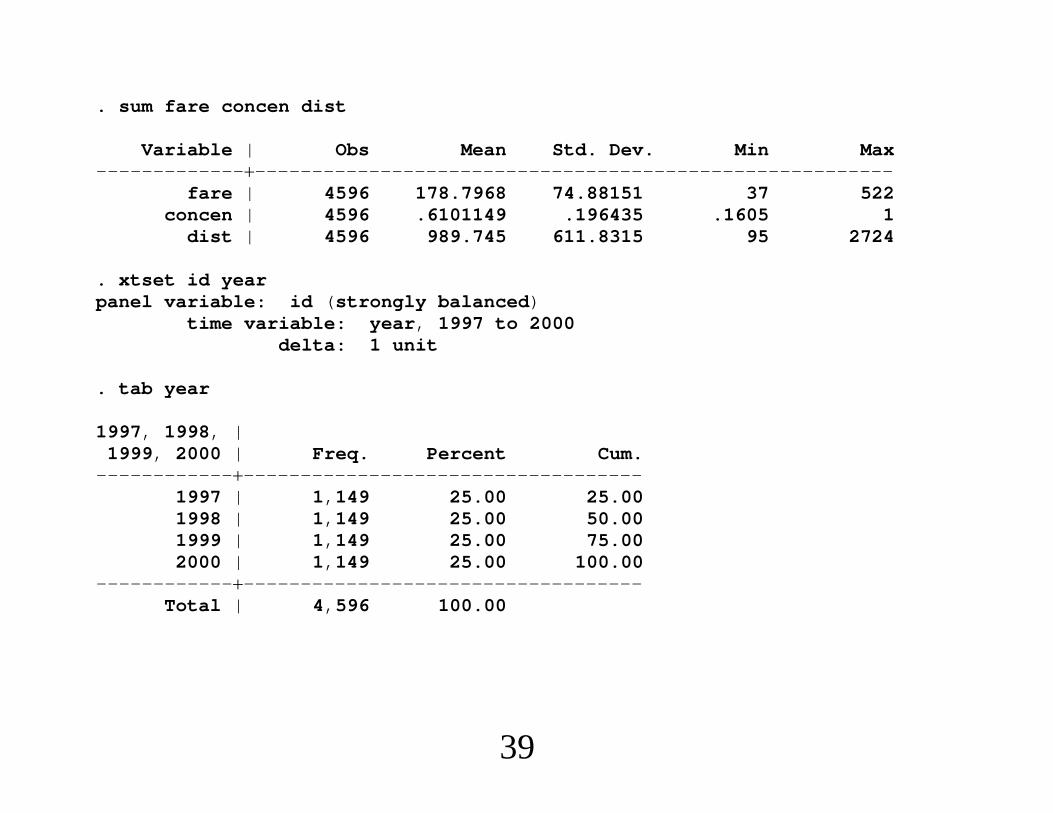
. sum fare concen dist
Variable | Obs Mean Std. Dev. Min Max---------------------------------------------------------------------
fare | 4596 178.7968 74.88151 37 522concen | 4596 .6101149 .196435 .1605 1
dist | 4596 989.745 611.8315 95 2724
. xtset id yearpanel variable: id (strongly balanced)
time variable: year, 1997 to 2000delta: 1 unit
. tab year
1997, 1998, |1999, 2000 | Freq. Percent Cum.
-----------------------------------------------1997 | 1,149 25.00 25.001998 | 1,149 25.00 50.001999 | 1,149 25.00 75.002000 | 1,149 25.00 100.00
-----------------------------------------------Total | 4,596 100.00
39

. reg lfare concen ldist ldistsq y98 y99 y00
Source | SS df MS Number of obs 4596------------------------------------------- F( 6, 4589) 523.
Model | 355.453858 6 59.2423096 Prob F 0.0000Residual | 519.640516 4589 .113236112 R-squared 0.4062
------------------------------------------- Adj R-squared 0.4054Total | 875.094374 4595 .190444913 Root MSE .33651
----------------------------------------------------------------------------lfare | Coef. Std. Err. t P|t| [95% Conf. Interval
---------------------------------------------------------------------------concen | .3601203 .0300691 11.98 0.000 .3011705 .4190702
ldist | -.9016004 .128273 -7.03 0.000 -1.153077 -.6501235ldistsq | .1030196 .0097255 10.59 0.000 .0839529 .1220863
y98 | .0211244 .0140419 1.50 0.133 -.0064046 .0486533y99 | .0378496 .0140413 2.70 0.007 .010322 .0653772y00 | .09987 .0140432 7.11 0.000 .0723385 .1274015
_cons | 6.209258 .4206247 14.76 0.000 5.384631 7.033884----------------------------------------------------------------------------
. * The above standard errors assume no serial correlation.
40

. reg lfare concen ldist ldistsq y98 y99 y00, cluster(id)
(Std. Err. adjusted for 1149 clusters in id----------------------------------------------------------------------------
| Robustlfare | Coef. Std. Err. t P|t| [95% Conf. Interval
---------------------------------------------------------------------------concen | .3601203 .058556 6.15 0.000 .2452315 .4750092
ldist | -.9016004 .2719464 -3.32 0.001 -1.435168 -.3680328ldistsq | .1030196 .0201602 5.11 0.000 .0634647 .1425745
y98 | .0211244 .0041474 5.09 0.000 .0129871 .0292617y99 | .0378496 .0051795 7.31 0.000 .0276872 .048012y00 | .09987 .0056469 17.69 0.000 .0887906 .1109493
_cons | 6.209258 .9117551 6.81 0.000 4.420364 7.998151----------------------------------------------------------------------------
. * Indirect evidence of plenty of serial correlation in the composite error
. * Other than introspection we have no way of knowing whether .360 is a
. * reliable estimate of the concentration effect.
41
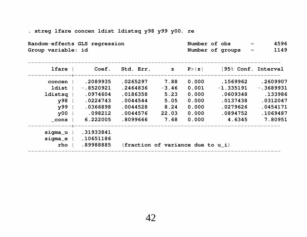
. xtreg lfare concen ldist ldistsq y98 y99 y00, re
Random-effects GLS regression Number of obs 4596Group variable: id Number of groups 1149
----------------------------------------------------------------------------lfare | Coef. Std. Err. z P|z| [95% Conf. Interval
---------------------------------------------------------------------------concen | .2089935 .0265297 7.88 0.000 .1569962 .2609907
ldist | -.8520921 .2464836 -3.46 0.001 -1.335191 -.3689931ldistsq | .0974604 .0186358 5.23 0.000 .0609348 .133986
y98 | .0224743 .0044544 5.05 0.000 .0137438 .0312047y99 | .0366898 .0044528 8.24 0.000 .0279626 .0454171y00 | .098212 .0044576 22.03 0.000 .0894752 .1069487
_cons | 6.222005 .8099666 7.68 0.000 4.6345 7.80951---------------------------------------------------------------------------
sigma_u | .31933841sigma_e | .10651186
rho | .89988885 (fraction of variance due to u_i)----------------------------------------------------------------------------
42
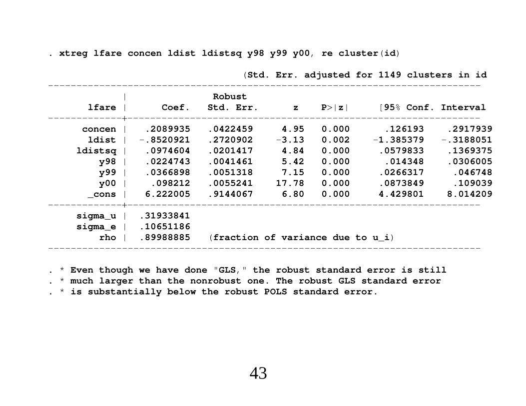
. xtreg lfare concen ldist ldistsq y98 y99 y00, re cluster(id)
(Std. Err. adjusted for 1149 clusters in id----------------------------------------------------------------------------
| Robustlfare | Coef. Std. Err. z P|z| [95% Conf. Interval
---------------------------------------------------------------------------concen | .2089935 .0422459 4.95 0.000 .126193 .2917939
ldist | -.8520921 .2720902 -3.13 0.002 -1.385379 -.3188051ldistsq | .0974604 .0201417 4.84 0.000 .0579833 .1369375
y98 | .0224743 .0041461 5.42 0.000 .014348 .0306005y99 | .0366898 .0051318 7.15 0.000 .0266317 .046748y00 | .098212 .0055241 17.78 0.000 .0873849 .109039
_cons | 6.222005 .9144067 6.80 0.000 4.429801 8.014209---------------------------------------------------------------------------
sigma_u | .31933841sigma_e | .10651186
rho | .89988885 (fraction of variance due to u_i)----------------------------------------------------------------------------
. * Even though we have done "GLS," the robust standard error is still
. * much larger than the nonrobust one. The robust GLS standard error
. * is substantially below the robust POLS standard error.
43
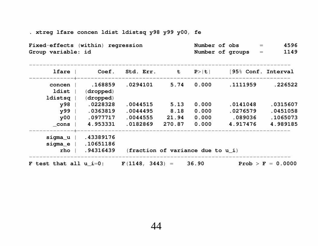
. xtreg lfare concen ldist ldistsq y98 y99 y00, fe
Fixed-effects (within) regression Number of obs 4596Group variable: id Number of groups 1149
----------------------------------------------------------------------------lfare | Coef. Std. Err. t P|t| [95% Conf. Interval
---------------------------------------------------------------------------concen | .168859 .0294101 5.74 0.000 .1111959 .226522
ldist | (dropped)ldistsq | (dropped)
y98 | .0228328 .0044515 5.13 0.000 .0141048 .0315607y99 | .0363819 .0044495 8.18 0.000 .0276579 .0451058y00 | .0977717 .0044555 21.94 0.000 .089036 .1065073
_cons | 4.953331 .0182869 270.87 0.000 4.917476 4.989185---------------------------------------------------------------------------
sigma_u | .43389176sigma_e | .10651186
rho | .94316439 (fraction of variance due to u_i)----------------------------------------------------------------------------F test that all u_i0: F(1148, 3443) 36.90 Prob F 0.0000
44
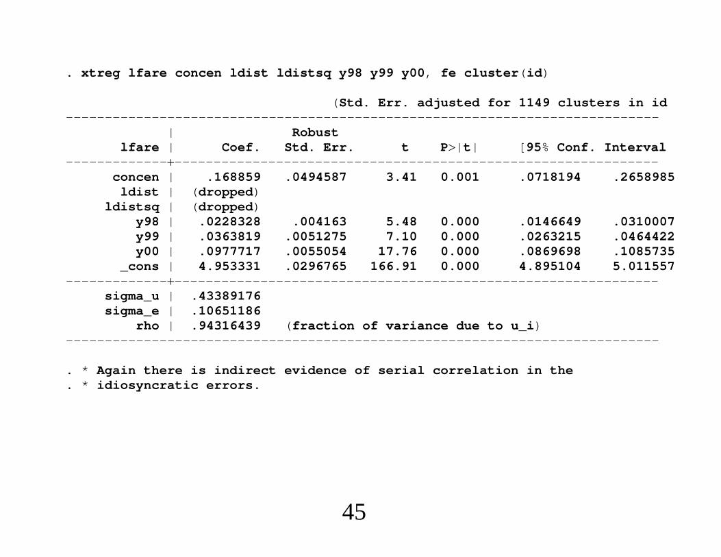
. xtreg lfare concen ldist ldistsq y98 y99 y00, fe cluster(id)
(Std. Err. adjusted for 1149 clusters in id----------------------------------------------------------------------------
| Robustlfare | Coef. Std. Err. t P|t| [95% Conf. Interval
---------------------------------------------------------------------------concen | .168859 .0494587 3.41 0.001 .0718194 .2658985
ldist | (dropped)ldistsq | (dropped)
y98 | .0228328 .004163 5.48 0.000 .0146649 .0310007y99 | .0363819 .0051275 7.10 0.000 .0263215 .0464422y00 | .0977717 .0055054 17.76 0.000 .0869698 .1085735
_cons | 4.953331 .0296765 166.91 0.000 4.895104 5.011557---------------------------------------------------------------------------
sigma_u | .43389176sigma_e | .10651186
rho | .94316439 (fraction of variance due to u_i)----------------------------------------------------------------------------
. * Again there is indirect evidence of serial correlation in the
. * idiosyncratic errors.
45
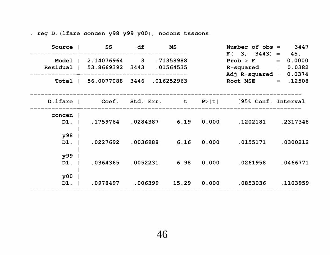
. reg D.(lfare concen y98 y99 y00), nocons tsscons
Source | SS df MS Number of obs 3447------------------------------------------- F( 3, 3443) 45.
Model | 2.14076964 3 .71358988 Prob F 0.0000Residual | 53.8669392 3443 .01564535 R-squared 0.0382
------------------------------------------- Adj R-squared 0.0374Total | 56.0077088 3446 .016252963 Root MSE .12508
----------------------------------------------------------------------------D.lfare | Coef. Std. Err. t P|t| [95% Conf. Interval
---------------------------------------------------------------------------concen |
D1. | .1759764 .0284387 6.19 0.000 .1202181 .2317348|
y98 |D1. | .0227692 .0036988 6.16 0.000 .0155171 .0300212
|y99 |D1. | .0364365 .0052231 6.98 0.000 .0261958 .0466771
|y00 |D1. | .0978497 .006399 15.29 0.000 .0853036 .1103959
----------------------------------------------------------------------------
46

. reg D.(lfare concen y98 y99 y00), nocons tsscons cluster(id)
Linear regression Number of obs 3447F( 3, 1148) 26.Prob F 0.0000
(Std. Err. adjusted for 1149 clusters in id----------------------------------------------------------------------------
| RobustD.lfare | Coef. Std. Err. t P|t| [95% Conf. Interval
---------------------------------------------------------------------------concen |
D1. | .1759764 .0430367 4.09 0.000 .0915371 .2604158|
y98 |D1. | .0227692 .0041573 5.48 0.000 .0146124 .030926
|y99 |D1. | .0364365 .005153 7.07 0.000 .026326 .0465469
|y00 |D1. | .0978497 .0055468 17.64 0.000 .0869666 .1087328
----------------------------------------------------------------------------
47

4. Comparing RE and FE∙ FE allows for correlation between ci and xit.∙ Time-constant variables drop out of FE estimation.Removes much of the covariate variation.∙ FE has more robustness to heterogeneous slopes.
48
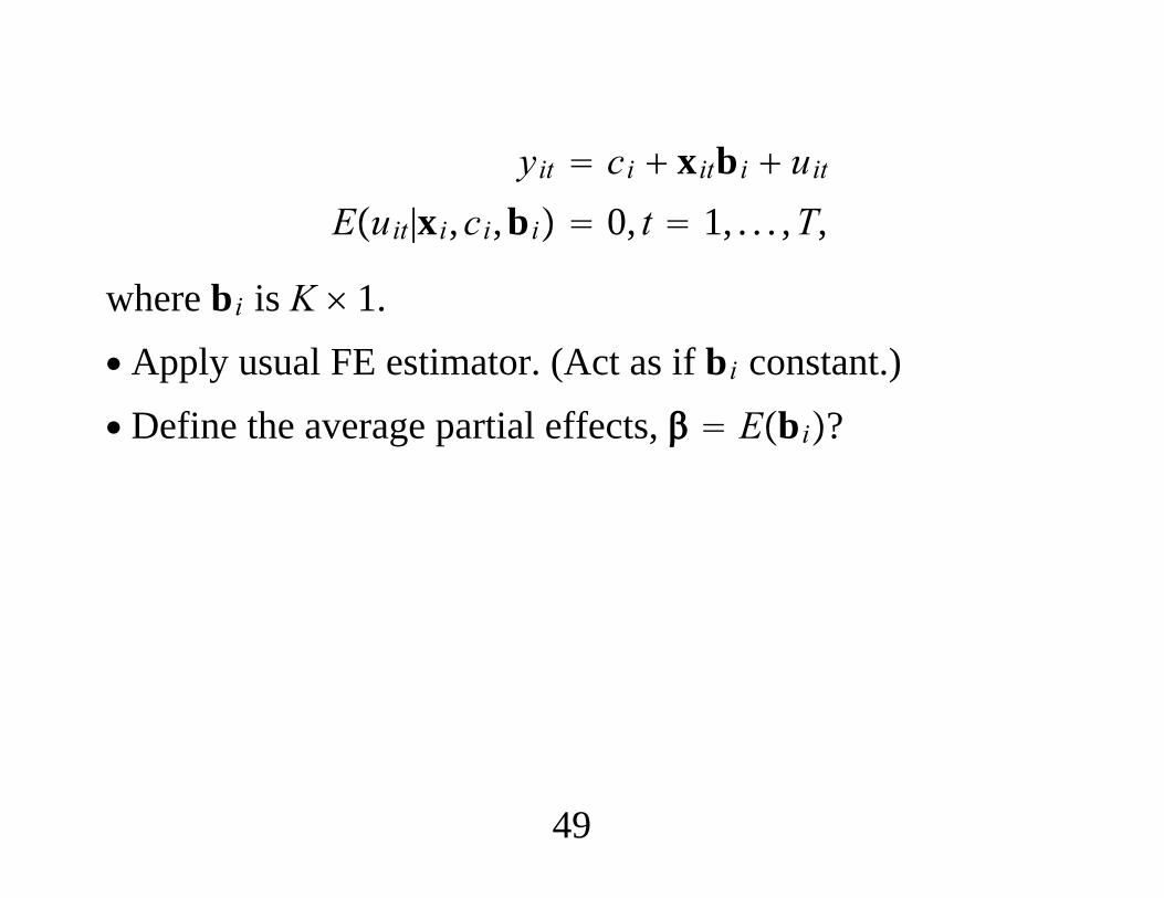
yit ci xitbi uitEuit|xi,ci,bi 0, t 1, . . . ,T,
where bi is K 1.∙ Apply usual FE estimator. (Act as if bi constant.)∙ Define the average partial effects, Ebi?
49
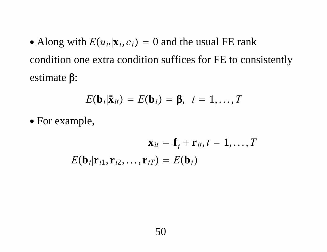
∙ Along with Euit|xi,ci 0 and the usual FE rankcondition one extra condition suffices for FE to consistentlyestimate :
Ebi|xit Ebi , t 1, . . . ,T
∙ For example,
xit fi rit, t 1, . . . ,TEbi|ri1,ri2, . . . ,riT Ebi
50
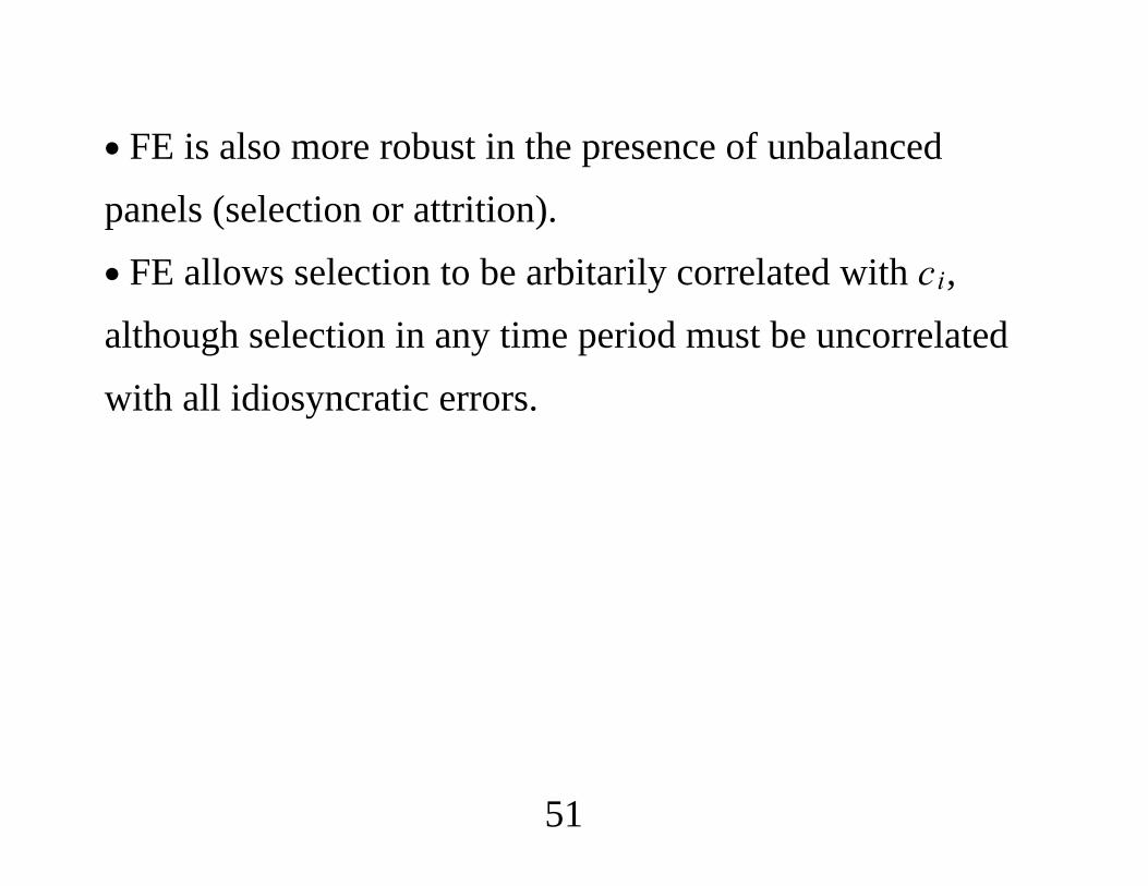
∙ FE is also more robust in the presence of unbalancedpanels (selection or attrition).∙ FE allows selection to be arbitarily correlated with ci,although selection in any time period must be uncorrelatedwith all idiosyncratic errors.
51
∙ How come RE and FE sometimes give similar estimates?∙ Define the parameter
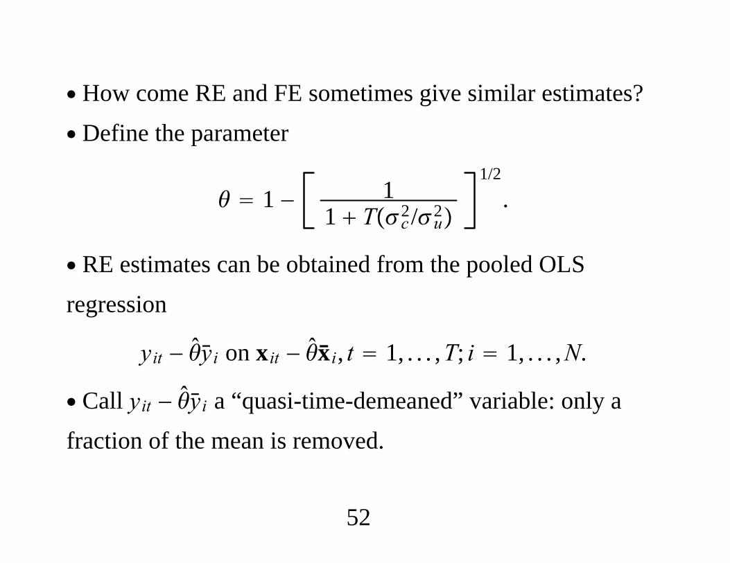
1 − 11 Tc2/u2
1/2
.
∙ RE estimates can be obtained from the pooled OLSregression
yit − yi on xit − xi, t 1, . . . ,T; i 1, . . . ,N.
∙ Call yit − yi a “quasi-time-demeaned” variable: only afraction of the mean is removed.
52
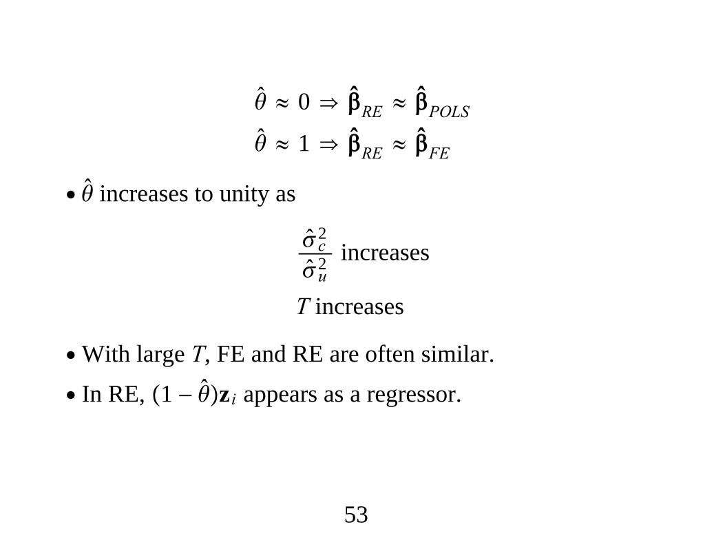
≈ 0 RE ≈ POLS ≈ 1 RE ≈ FE
∙ increases to unity as
c2
u2increases
T increases
∙With large T, FE and RE are often similar.
∙ In RE, 1 − zi appears as a regressor.
53
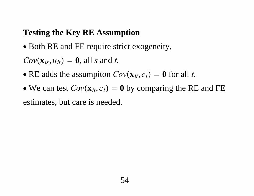
Testing the Key RE Assumption∙ Both RE and FE require strict exogeneity,Covxis,uit 0, all s and t.∙ RE adds the assumpiton Covxit,ci 0 for all t.∙We can test Covxit,ci 0 by comparing the RE and FEestimates, but care is needed.
54
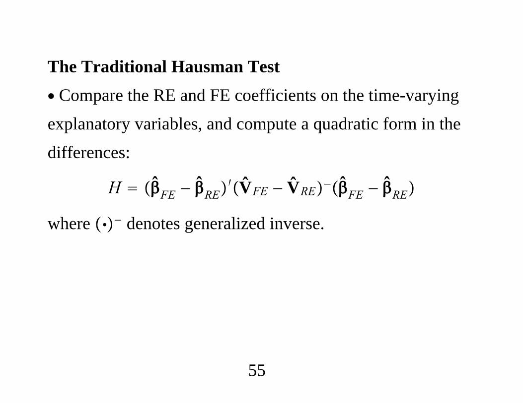
The Traditional Hausman Test∙ Compare the RE and FE coefficients on the time-varyingexplanatory variables, and compute a quadratic form in thedifferences:
H FE − RE′VFE − VRE−FE − RE
where − denotes generalized inverse.
55
∙ Cautions1. Usual Hausman test maintains the RE second momentassumptions yet has no systematic power for detectingviolations of these assumptions.2. With time dummies (aggregate time effects), must usegeneralized inverse.3. Easy to get the degrees of freedom wrong with aggregatetime effects.
56

Variable Addition Test (VAT)∙Write the model as
yit gt zi wit ci uit.
∙ Cannot compare FE and RE estimates of .∙ Less obvious: Cannot compare FE and RE estimates of .
We can obtain FE and RE, but there is a degeneracy.∙We can only compare FE and RE.
57
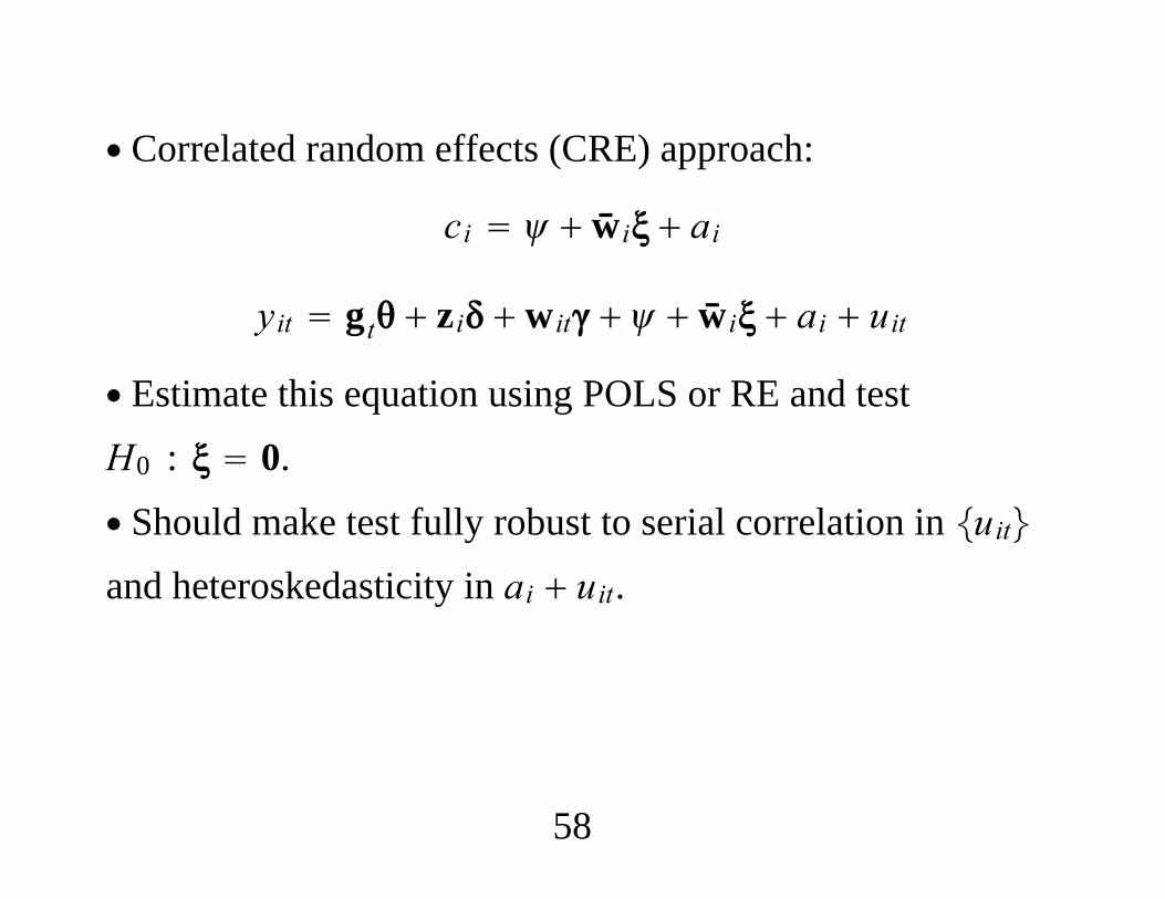
∙ Correlated random effects (CRE) approach:
ci wi ai
yit gt zi wit wi ai uit
∙ Estimate this equation using POLS or RE and testH0 : 0.
∙ Should make test fully robust to serial correlation in uitand heteroskedasticity in ai uit.
58

∙ Important Algebraic Result: The RE estimate of ,
when wi is included is the FE estimate.∙ POLS and RE of all coefficients with wi are identical.∙ Including wi effectively proxies for ci (even though ai isstill in error term).∙ Implication of Algebraic Result: Test is valid for anyrelationship between ci and wi1,wi2, . . . ,wiT.
59
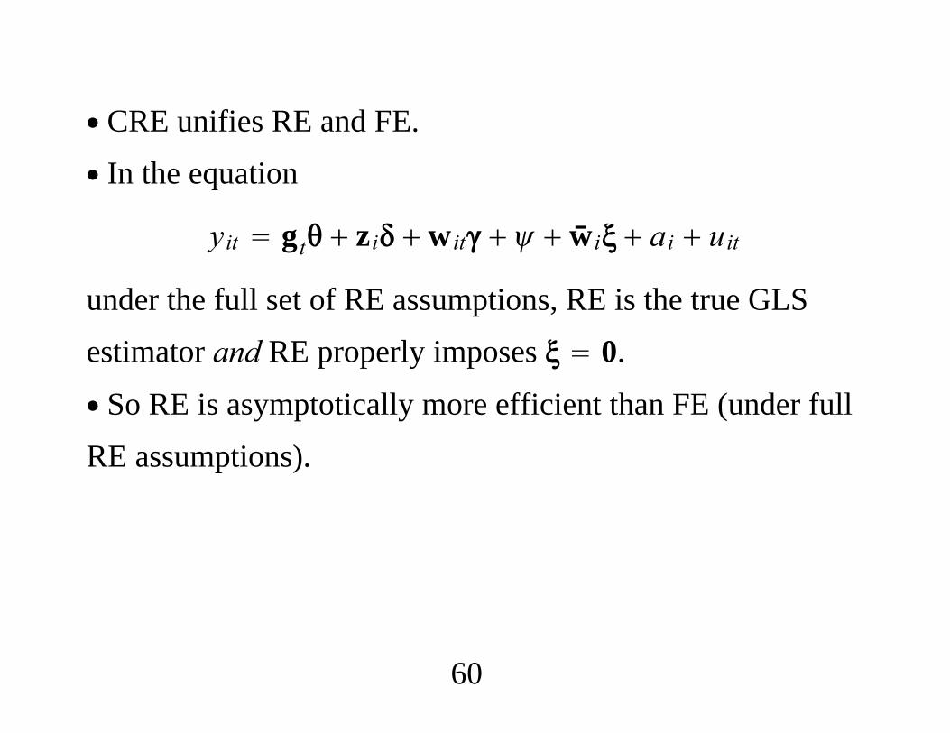
∙ CRE unifies RE and FE.∙ In the equation
yit gt zi wit wi ai uit
under the full set of RE assumptions, RE is the true GLSestimator and RE properly imposes 0.
∙ So RE is asymptotically more efficient than FE (under fullRE assumptions).
60
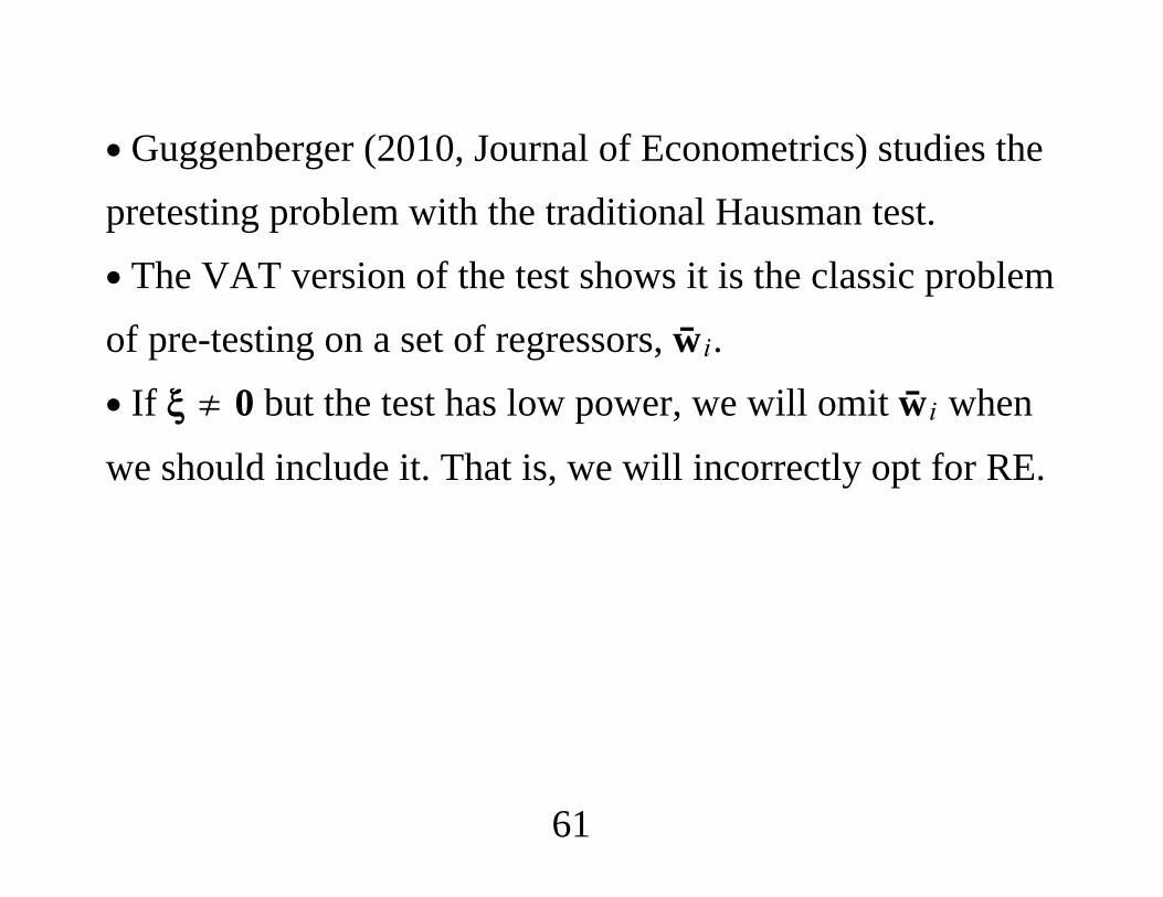
∙ Guggenberger (2010, Journal of Econometrics) studies thepretesting problem with the traditional Hausman test.∙ The VAT version of the test shows it is the classic problemof pre-testing on a set of regressors, wi.∙ If ≠ 0 but the test has low power, we will omit wi when
we should include it. That is, we will incorrectly opt for RE.
61

∙ Apply to airfare model:. * First use the Hausman test that maintains all of the RE assumptions under. * the null:
. qui xtreg lfare concen ldist ldistsq y98 y99 y00, fe
. estimates store b_fe
. qui xtreg lfare concen ldist ldistsq y98 y99 y00, re
. estimates store b_re
62
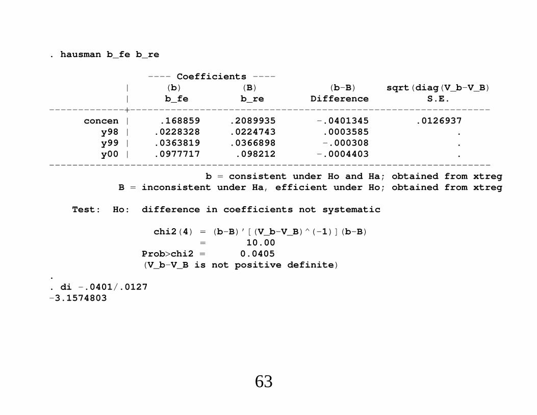
. hausman b_fe b_re
---- Coefficients ----| (b) (B) (b-B) sqrt(diag(V_b-V_B)| b_fe b_re Difference S.E.
---------------------------------------------------------------------------concen | .168859 .2089935 -.0401345 .0126937
y98 | .0228328 .0224743 .0003585 .y99 | .0363819 .0366898 -.000308 .y00 | .0977717 .098212 -.0004403 .
----------------------------------------------------------------------------b consistent under Ho and Ha; obtained from xtreg
B inconsistent under Ha, efficient under Ho; obtained from xtreg
Test: Ho: difference in coefficients not systematic
chi2(4) (b-B)’[(V_b-V_B)^(-1)](b-B) 10.00
Probchi2 0.0405(V_b-V_B is not positive definite)
.
. di -.0401/.0127-3.1574803
63
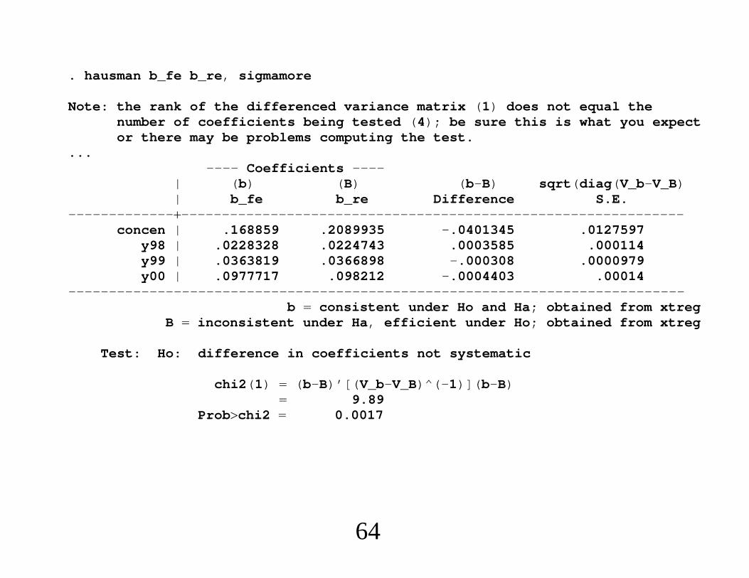
. hausman b_fe b_re, sigmamore
Note: the rank of the differenced variance matrix (1) does not equal thenumber of coefficients being tested (4); be sure this is what you expector there may be problems computing the test.
...---- Coefficients ----
| (b) (B) (b-B) sqrt(diag(V_b-V_B)| b_fe b_re Difference S.E.
---------------------------------------------------------------------------concen | .168859 .2089935 -.0401345 .0127597
y98 | .0228328 .0224743 .0003585 .000114y99 | .0363819 .0366898 -.000308 .0000979y00 | .0977717 .098212 -.0004403 .00014
----------------------------------------------------------------------------b consistent under Ho and Ha; obtained from xtreg
B inconsistent under Ha, efficient under Ho; obtained from xtreg
Test: Ho: difference in coefficients not systematic
chi2(1) (b-B)’[(V_b-V_B)^(-1)](b-B) 9.89
Probchi2 0.0017
64

. egen concenbar mean(concen), by(id)
. xtreg lfare concen concenbar ldist ldistsq y98 y99 y00, re cluster(id)
(Std. Err. adjusted for 1149 clusters in id----------------------------------------------------------------------------
| Robustlfare | Coef. Std. Err. z P|z| [95% Conf. Interval
---------------------------------------------------------------------------concen | .168859 .0494749 3.41 0.001 .07189 .2658279
concenbar | .2136346 .0816403 2.62 0.009 .0536227 .3736466ldist | -.9089297 .2721637 -3.34 0.001 -1.442361 -.3754987
ldistsq | .1038426 .0201911 5.14 0.000 .0642688 .1434164y98 | .0228328 .0041643 5.48 0.000 .0146708 .0309947y99 | .0363819 .0051292 7.09 0.000 .0263289 .0464349y00 | .0977717 .0055072 17.75 0.000 .0869777 .1085656
_cons | 6.207889 .9118109 6.81 0.000 4.420773 7.995006---------------------------------------------------------------------------
sigma_u | .31933841sigma_e | .10651186
rho | .89988885 (fraction of variance due to u_i)----------------------------------------------------------------------------
. * The robust t statistic is 2.62 --- still a rejection, but not as strong.
65

Coefficients on Time-Constant Variables∙What if in
yit gt zi wit ci uit
we assume
Covzi,ci 0
but want to allow
Covwit,ci ≠ 0?
66

∙ Simple estimator: Use 1,gt,zi, wit as instruments in a
pooled IV procedure. Special case of Hausman-Taylor.∙ The estimator of , is the usual FE estimator.
∙ Use cluster-robust inference.∙ Contrast with the CRE approach: POLS (RE) applied to
yit gt zi wit wi ai uit,
which partials out wi.∙ Identical to pooled IV with instruments 1,gt,zi, wit, wi.
67
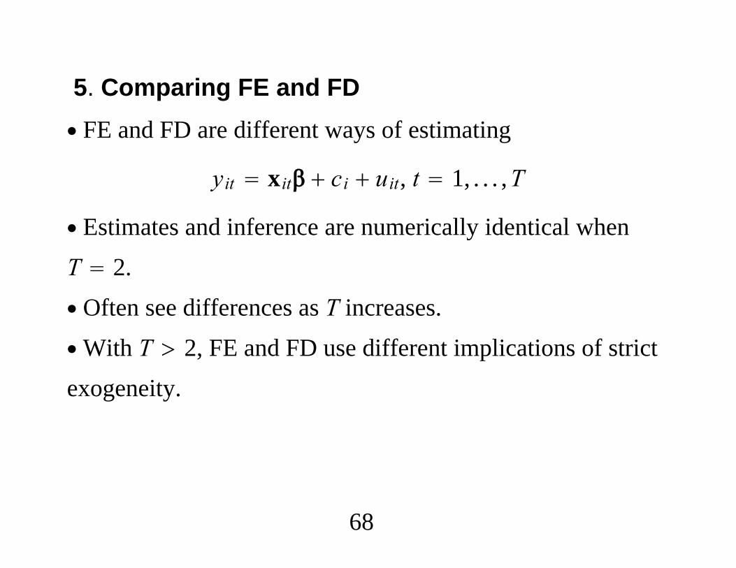
5. Comparing FE and FD∙ FE and FD are different ways of estimating
yit xit ci uit, t 1, . . . ,T
∙ Estimates and inference are numerically identical whenT 2.∙ Often see differences as T increases.∙With T 2, FE and FD use different implications of strictexogeneity.
68
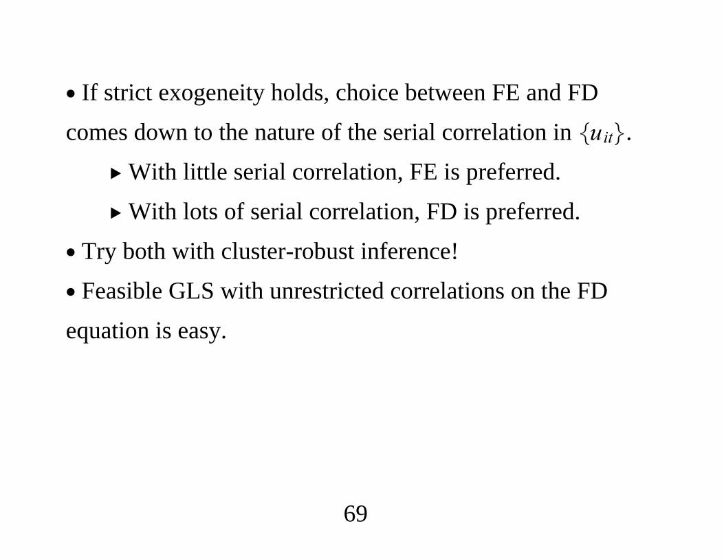
∙ If strict exogeneity holds, choice between FE and FDcomes down to the nature of the serial correlation in uit.
With little serial correlation, FE is preferred. With lots of serial correlation, FD is preferred.
∙ Try both with cluster-robust inference!∙ Feasible GLS with unrestricted correlations on the FDequation is easy.
69
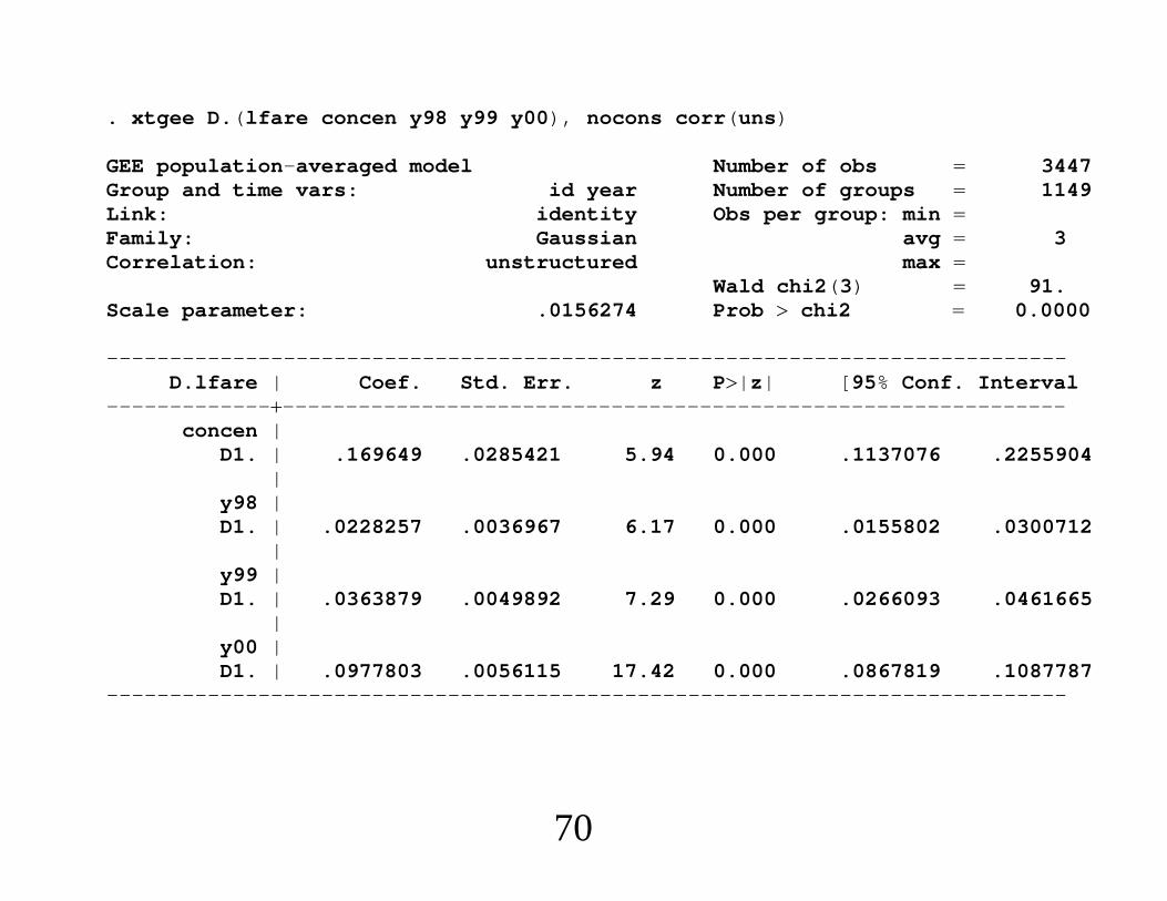
. xtgee D.(lfare concen y98 y99 y00), nocons corr(uns)
GEE population-averaged model Number of obs 3447Group and time vars: id year Number of groups 1149Link: identity Obs per group: min Family: Gaussian avg 3Correlation: unstructured max
Wald chi2(3) 91.Scale parameter: .0156274 Prob chi2 0.0000
----------------------------------------------------------------------------D.lfare | Coef. Std. Err. z P|z| [95% Conf. Interval
---------------------------------------------------------------------------concen |
D1. | .169649 .0285421 5.94 0.000 .1137076 .2255904|
y98 |D1. | .0228257 .0036967 6.17 0.000 .0155802 .0300712
|y99 |D1. | .0363879 .0049892 7.29 0.000 .0266093 .0461665
|y00 |D1. | .0977803 .0056115 17.42 0.000 .0867819 .1087787
----------------------------------------------------------------------------
70
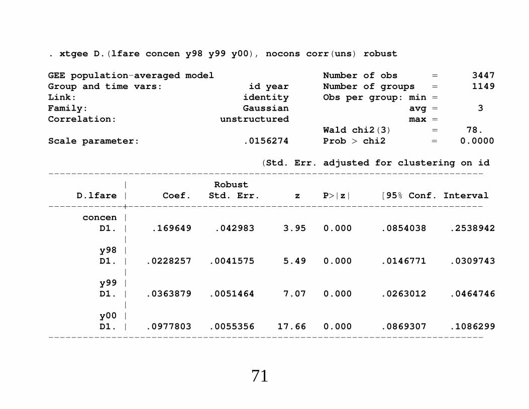
. xtgee D.(lfare concen y98 y99 y00), nocons corr(uns) robust
GEE population-averaged model Number of obs 3447Group and time vars: id year Number of groups 1149Link: identity Obs per group: min Family: Gaussian avg 3Correlation: unstructured max
Wald chi2(3) 78.Scale parameter: .0156274 Prob chi2 0.0000
(Std. Err. adjusted for clustering on id----------------------------------------------------------------------------
| RobustD.lfare | Coef. Std. Err. z P|z| [95% Conf. Interval
---------------------------------------------------------------------------concen |
D1. | .169649 .042983 3.95 0.000 .0854038 .2538942|
y98 |D1. | .0228257 .0041575 5.49 0.000 .0146771 .0309743
|y99 |D1. | .0363879 .0051464 7.07 0.000 .0263012 .0464746
|y00 |D1. | .0977803 .0055356 17.66 0.000 .0869307 .1086299
----------------------------------------------------------------------------
71
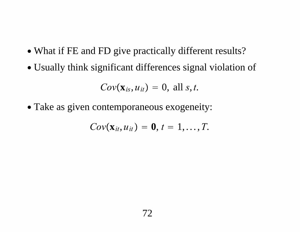
∙What if FE and FD give practically different results?∙ Usually think significant differences signal violation of
Covxis,uit 0, all s, t.
∙ Take as given contemporaneous exogeneity:
Covxit,uit 0, t 1, . . . ,T.
72
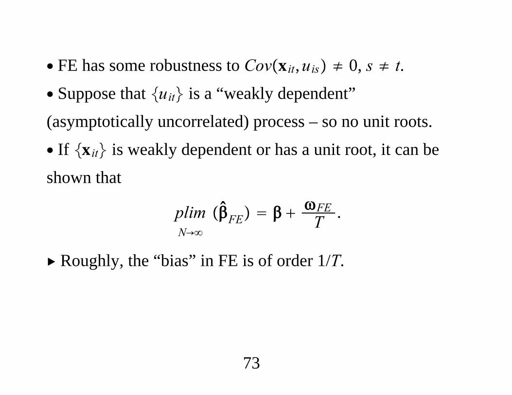
∙ FE has some robustness to Covxit,uis ≠ 0, s ≠ t.∙ Suppose that uit is a “weakly dependent”(asymptotically uncorrelated) process – so no unit roots.∙ If xit is weakly dependent or has a unit root, it can beshown that
N→plim FE FE
T .
Roughly, the “bias” in FE is of order 1/T.
73
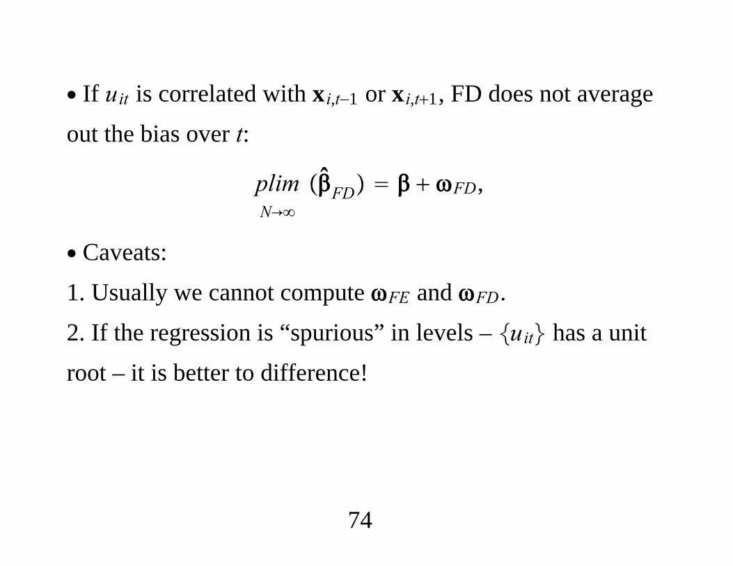
∙ If uit is correlated with xi,t−1 or xi,t1, FD does not averageout the bias over t:
N→plim FD FD,
∙ Caveats:1. Usually we cannot compute FE and FD.2. If the regression is “spurious” in levels – uit has a unitroot – it is better to difference!
74
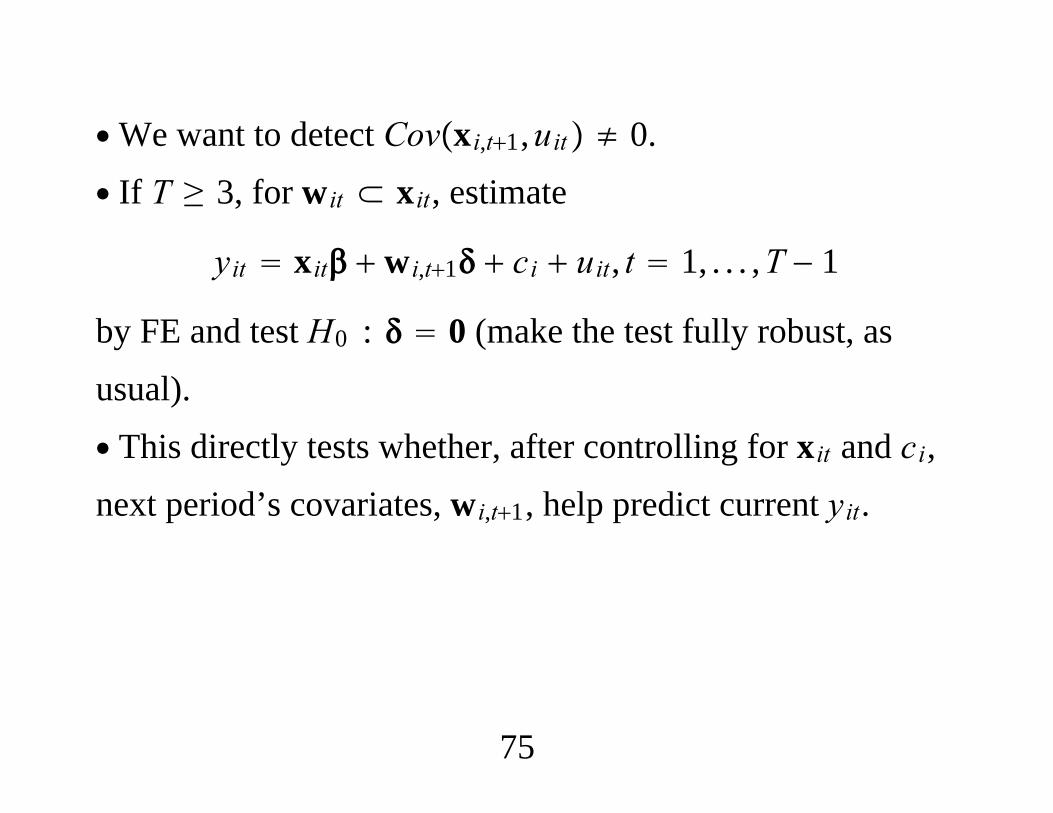
∙We want to detect Covxi,t1,uit ≠ 0.∙ If T ≥ 3, for wit ⊂ xit, estimate
yit xit wi,t1 ci uit, t 1, . . . ,T − 1
by FE and test H0 : 0 (make the test fully robust, asusual).∙ This directly tests whether, after controlling for xit and ci,next period’s covariates, wi,t1, help predict current yit.
75
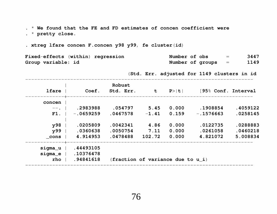
. * We found that the FE and FD estimates of concen coefficient were
. * pretty close.
. xtreg lfare concen F.concen y98 y99, fe cluster(id)
Fixed-effects (within) regression Number of obs 3447Group variable: id Number of groups 1149
(Std. Err. adjusted for 1149 clusters in id----------------------------------------------------------------------------
| Robustlfare | Coef. Std. Err. t P|t| [95% Conf. Interval
---------------------------------------------------------------------------concen |
--. | .2983988 .054797 5.45 0.000 .1908854 .4059122F1. | -.0659259 .0467578 -1.41 0.159 -.1576663 .0258145
|y98 | .0205809 .0042341 4.86 0.000 .0122735 .0288883y99 | .0360638 .0050754 7.11 0.000 .0261058 .0460218
_cons | 4.914953 .0478488 102.72 0.000 4.821072 5.008834---------------------------------------------------------------------------
sigma_u | .44493105sigma_e | .10376478
rho | .94841618 (fraction of variance due to u_i)----------------------------------------------------------------------------
76

Econometrics of Cross Section and Panel DataLecture 4: Linear Panel Data Models II
Jeff WooldridgeMichigan State University
cemmap/PEPA, June 2014
1. Linear Models under Sequential Exogeneity2. Estimating Production Functions Using Proxy Variables3. Pseudo Panels from Pooled Cross Sections
1
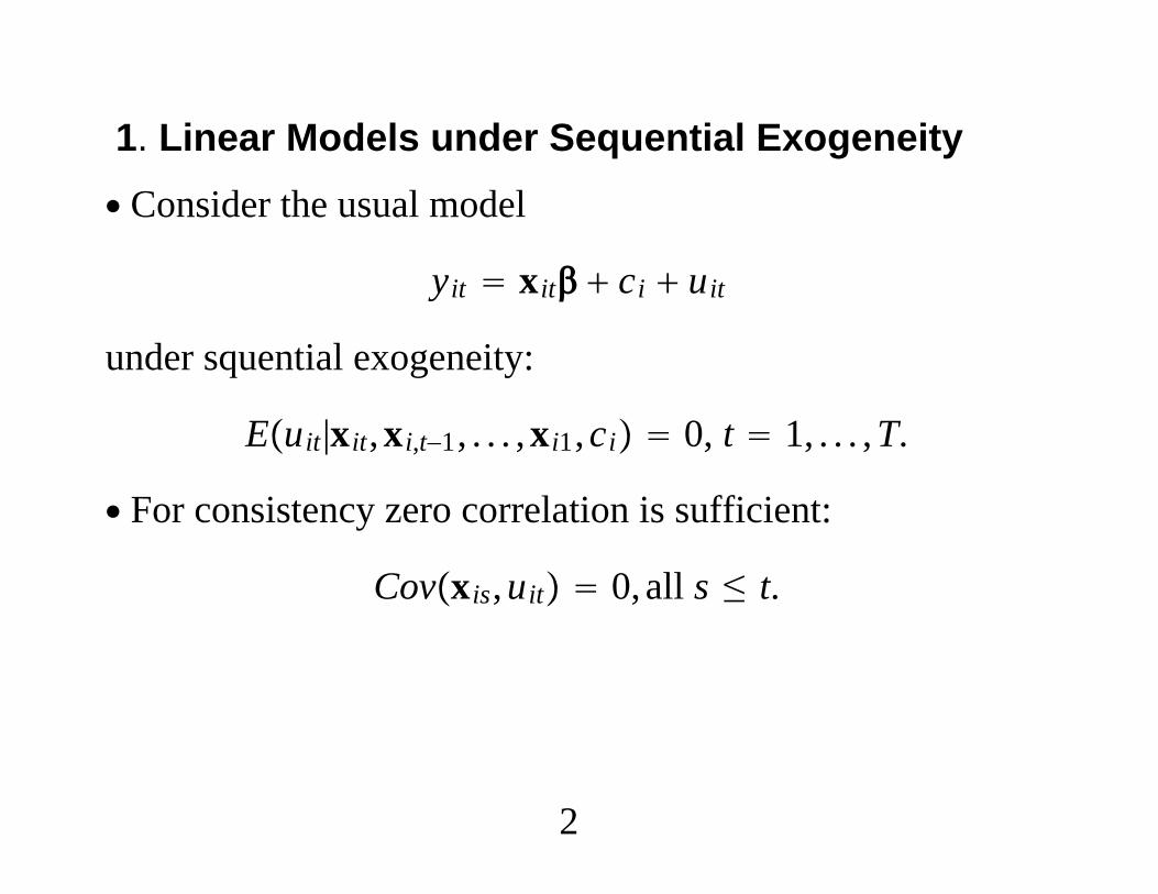
1. Linear Models under Sequential Exogeneity∙ Consider the usual model
yit xit ci uit
under squential exogeneity:
Euit|xit,xi,t−1, . . . ,xi1,ci 0, t 1, . . . ,T.
∙ For consistency zero correlation is sufficient:
Covxis,uit 0, all s ≤ t.
2
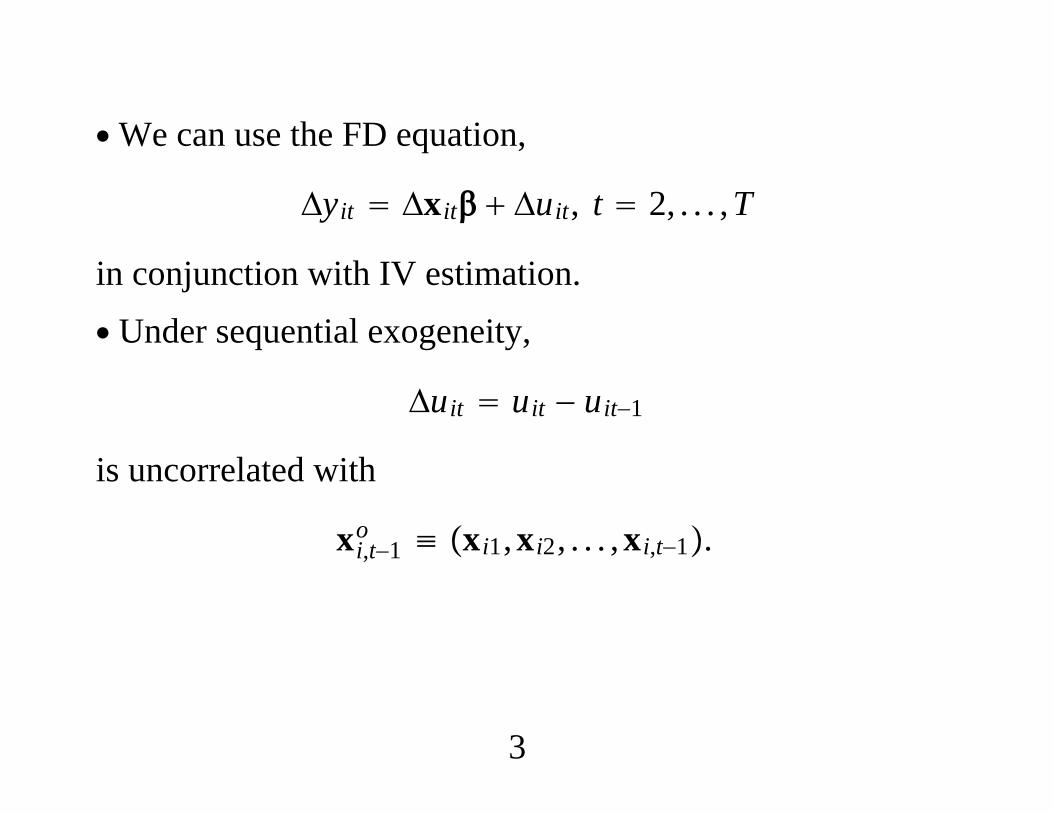
∙We can use the FD equation,
Δyit Δxit Δuit, t 2, . . . ,T
in conjunction with IV estimation.∙ Under sequential exogeneity,
Δuit uit − uit−1
is uncorrelated with
xi,t−1o ≡ xi1,xi2, . . . ,xi,t−1.
3

∙We have the moment conditions
Exi,t−1o′ Δuit 0, t 2, . . . ,T.
∙ Fairly routine to apply GMM estimation.∙ For each t, first run the reduced form regressions
Δxit on xi,t−1o , i 1, . . . ,N
to determine if there is a “weak instrument” problem.
4

∙ If Δxit is the 1 K vector of fitted values, can use these asIVs (not regressors!) in the equation
Δyit Δxit Δuit, t 2, . . . ,T
∙ Just pooled IV using serial correlation-roust inference.
5

∙ One case where xi,t−1o are irrelevant instruments for Δxit:
xit t xi,t−1 rit
Erit|xi,t−1,xi,t−2, . . . ,xi0 0
∙ Then EΔxit|xi,t−1o EΔxit t, and IV in a model with
time effects fails.∙ One solution to the weak instrument problem is to searchfor more moment conditions.
6

∙ Arellano and Bover (1995) suggested adding
CovΔxit′ ,ci 0, t 2, . . . ,T.
∙ Suppose xit follows
xit fi rit
Then sufficient is
Covrit,ci 0, t 1, 2, . . .
∙ Covfi,ci is unrestricted.
7
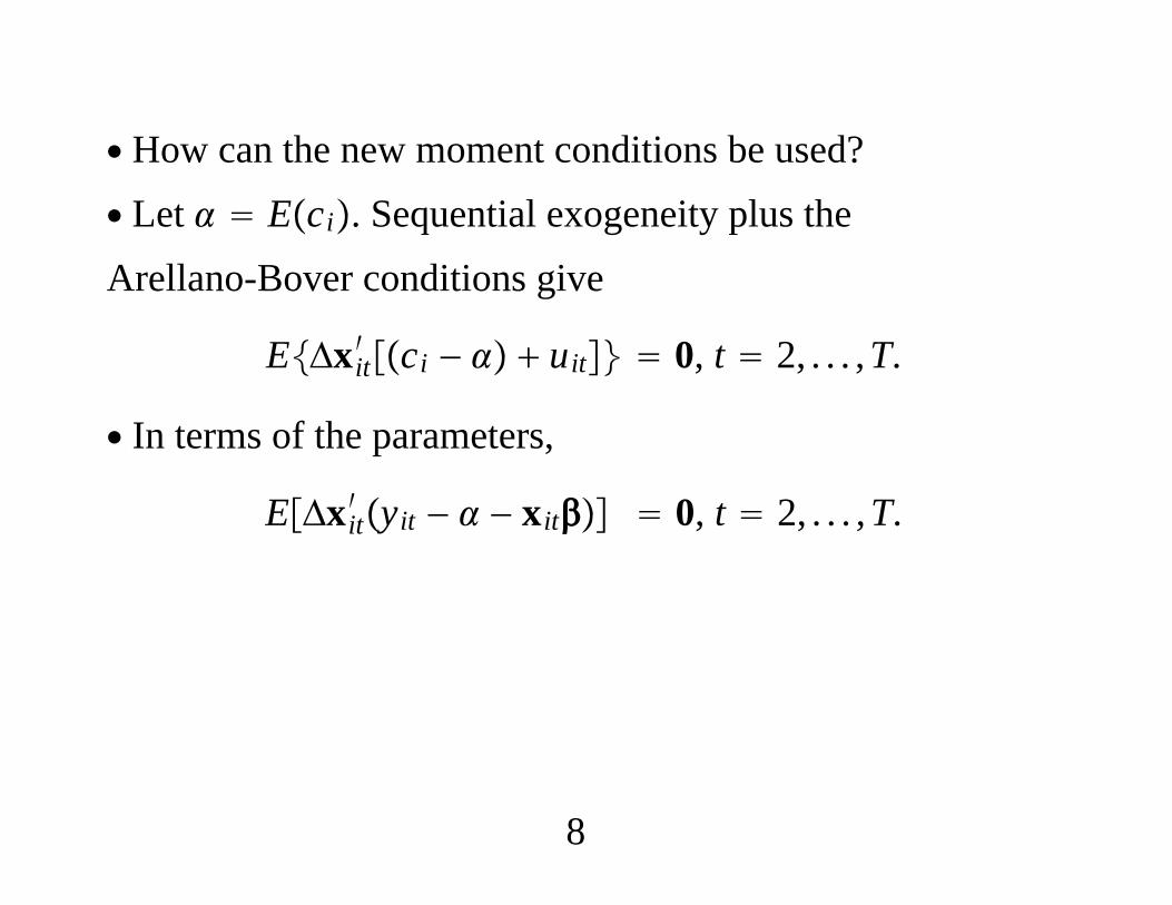
∙ How can the new moment conditions be used?∙ Let Eci. Sequential exogeneity plus theArellano-Bover conditions give
EΔxit′ ci − uit 0, t 2, . . . ,T.
∙ In terms of the parameters,
EΔxit′ yit − − xit 0, t 2, . . . ,T.
8
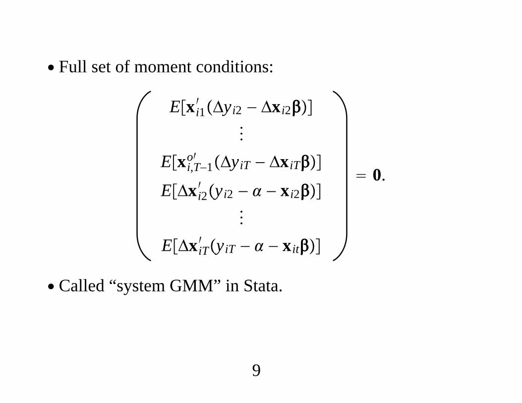
∙ Full set of moment conditions:
Exi1′ Δyi2 − Δxi2
Exi,T−1o′ ΔyiT − ΔxiT
EΔxi2′ yi2 − − xi2
EΔxiT′ yiT − − xit
0.
∙ Called “system GMM” in Stata.
9
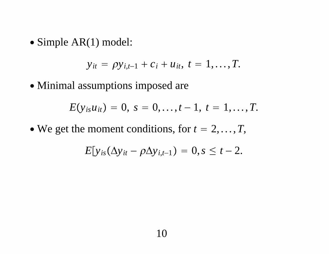
∙ Simple AR(1) model:
yit yi,t−1 ci uit, t 1, . . . ,T.
∙Minimal assumptions imposed are
Eyisuit 0, s 0, . . . , t − 1, t 1, . . . ,T.
∙We get the moment conditions, for t 2, . . . ,T,
EyisΔyit − Δyi,t−1 0, s ≤ t − 2.
10
∙ Can suffer from weak instruments when is close to unity.
∙ Blundell and Bond (1998) showed that if
Covyi1 − yi0,ci 0
is added then the Arellano and Bover condition holds:
EΔyi,t−1yit − − yi,t−1 0.
11
∙ Extensions of the AR(1) model,
yit yi,t−1 zit ci uit, t 1, . . . ,T
are easily handled using FD:
Δyit Δyi,t−1 Δzit Δuit, t 2, . . . ,TEyisΔuit 0, s ≤ t − 2
∙ Can use Δzit as own IVs if they are strictly exogenous.
12

∙ If zit is not strictly exogenous, can use zi,t−1, . . . ,zi1 asIVs, along with yi,t−2, . . . ,yi0 in the FD equation at time t.∙ And, we still might use, for t 2, . . . ,T, momentconditions on the levels:
EΔyi,t−1yit − − yi,t−1 − zit 0EΔzit
′ yit − − yi,t−1 − zit 0
∙ Airfare Example:
lfareit t lfarei,t−1 concenit cit uit
13

Dep. Var. lfare(1) (2) (3) (4)
Expl. Var. FD-OLS FE FD-IV A-Blfare−1
.027−. 126
.032. 077
.062. 219
.055. 333
concen.053. 076
.053. 058
.056. 126
.040. 152
N 1, 149 1, 149 1, 149 1, 149
14
. gen dlfare d.lfare(1149 missing values generated). gen dlfare_1 l.dlfare(2298 missing values generated). gen dconcen d.concen(1149 missing values generated)
. reg dlfare dlfare_1 dconcen y99, cluster(id)
Linear regression Number of obs 2298
(Std. Err. adjusted for 1149 clusters in id----------------------------------------------------------------------------
| Robustdlfare | Coef. Std. Err. t P|t| [95% Conf. Interval
---------------------------------------------------------------------------dlfare_1 | -.1264673 .0267104 -4.73 0.000 -.1788739 -.0740606
dconcen | .0762671 .0527226 1.45 0.148 -.0271763 .1797106y99 | -.0473536 .0050308 -9.41 0.000 -.0572241 -.037483
_cons | .0624434 .0032977 18.94 0.000 .0559732 .0689136----------------------------------------------------------------------------
15
. xtreg lfare lfare_1 concen y99 y00, fe cluster(id)
Fixed-effects (within) regression Number of obs 3447Group variable: id Number of groups 1149
(Std. Err. adjusted for 1149 clusters in id----------------------------------------------------------------------------
| Robustlfare | Coef. Std. Err. t P|t| [95% Conf. Interval
---------------------------------------------------------------------------lfare_1 | .0773594 .0318913 2.43 0.015 .0147877 .1399311
concen | .0579086 .0533893 1.08 0.278 -.0468428 .1626601y99 | .0098236 .0037176 2.64 0.008 .0025296 .0171177y00 | .0700164 .0043967 15.92 0.000 .06139 .0786428
_cons | 4.653928 .1628858 28.57 0.000 4.334341 4.973515---------------------------------------------------------------------------
sigma_u | .38891209sigma_e | .09055856
rho | .94856899 (fraction of variance due to u_i)----------------------------------------------------------------------------
16
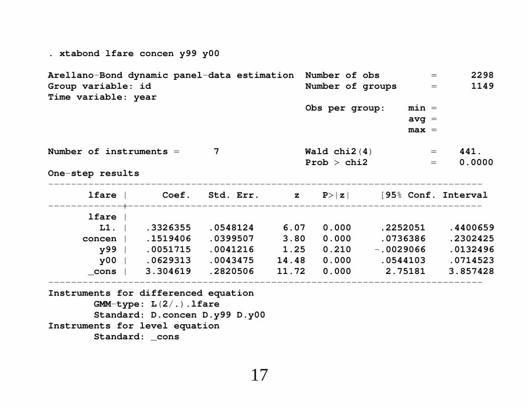
. xtabond lfare concen y99 y00
Arellano-Bond dynamic panel-data estimation Number of obs 2298Group variable: id Number of groups 1149Time variable: year
Obs per group: min avg max
Number of instruments 7 Wald chi2(4) 441.Prob chi2 0.0000
One-step results----------------------------------------------------------------------------
lfare | Coef. Std. Err. z P|z| [95% Conf. Interval---------------------------------------------------------------------------
lfare |L1. | .3326355 .0548124 6.07 0.000 .2252051 .4400659
concen | .1519406 .0399507 3.80 0.000 .0736386 .2302425y99 | .0051715 .0041216 1.25 0.210 -.0029066 .0132496y00 | .0629313 .0043475 14.48 0.000 .0544103 .0714523
_cons | 3.304619 .2820506 11.72 0.000 2.75181 3.857428----------------------------------------------------------------------------Instruments for differenced equation
GMM-type: L(2/.).lfareStandard: D.concen D.y99 D.y00
Instruments for level equationStandard: _cons
17
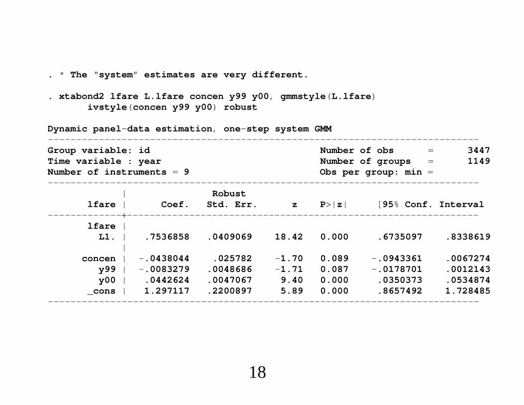
. * The “system” estimates are very different.
. xtabond2 lfare L.lfare concen y99 y00, gmmstyle(L.lfare)ivstyle(concen y99 y00) robust
Dynamic panel-data estimation, one-step system GMM----------------------------------------------------------------------------Group variable: id Number of obs 3447Time variable : year Number of groups 1149Number of instruments 9 Obs per group: min ----------------------------------------------------------------------------
| Robustlfare | Coef. Std. Err. z P|z| [95% Conf. Interval
---------------------------------------------------------------------------lfare |
L1. | .7536858 .0409069 18.42 0.000 .6735097 .8338619|
concen | -.0438044 .025782 -1.70 0.089 -.0943361 .0067274y99 | -.0083279 .0048686 -1.71 0.087 -.0178701 .0012143y00 | .0442624 .0047067 9.40 0.000 .0350373 .0534874
_cons | 1.297117 .2200897 5.89 0.000 .8657492 1.728485----------------------------------------------------------------------------
18

2. Estimating Production Functions Using ProxyVariables∙ Olley and Pakes (1996) show how investment can be usedas a proxy variable for unobserved, time-varyingproductivity.∙ Productivity can be expressed as an unknown function ofcapital and investment (when investment is strictly positive).∙ Approach does not assume inputs are strictly exogenous(but omits firm heterogeneity).
19
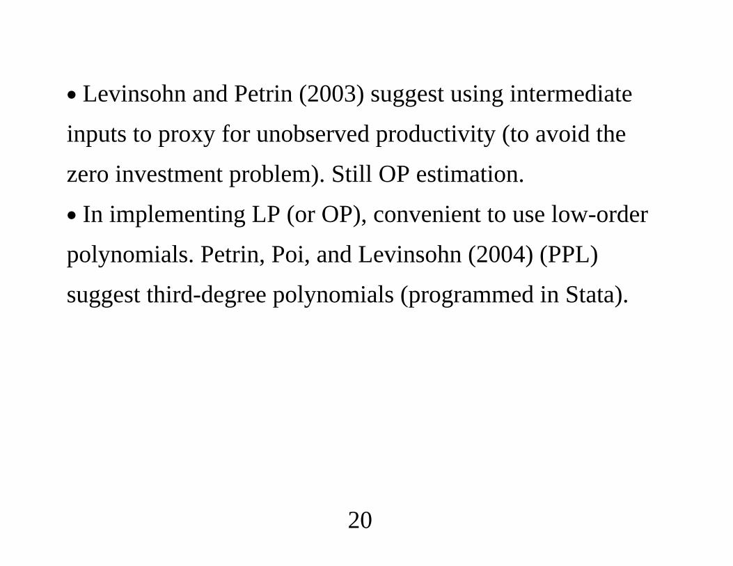
∙ Levinsohn and Petrin (2003) suggest using intermediateinputs to proxy for unobserved productivity (to avoid thezero investment problem). Still OP estimation.∙ In implementing LP (or OP), convenient to use low-orderpolynomials. Petrin, Poi, and Levinsohn (2004) (PPL)suggest third-degree polynomials (programmed in Stata).
20

∙Wooldridge (2009, Economics Letters): Set up as atwo-equation system for panel data with the same dependentvariable, but where the set of instruments differs acrossequation.∙ Simpler, more efficient, leads to insights aboutidentification.
21

∙ Production function for firm i in period t:
yit lit kit vit eit, t 1, . . . ,T, (1)
yit logarithm of the firm’s outputlit 1 J vector of variable inputs (labor)
kit 1 K vector of observed state variables (capital)
∙ vit : t 1, . . . ,T is unobserved productivity andeit : t 1, 2, . . . ,T is a sequence of shocks.
22

∙ Key implication of the theory underlying OP and LP: Forsome function g, ,
vit gkit,mit, t 1, . . . ,T, (2)
where mit is a 1 M vector of proxy variables.∙ In OP, mit consists of investment; in LP, mit isintermediate inputs.∙ Can somewhat relax time invariance of g, .
23
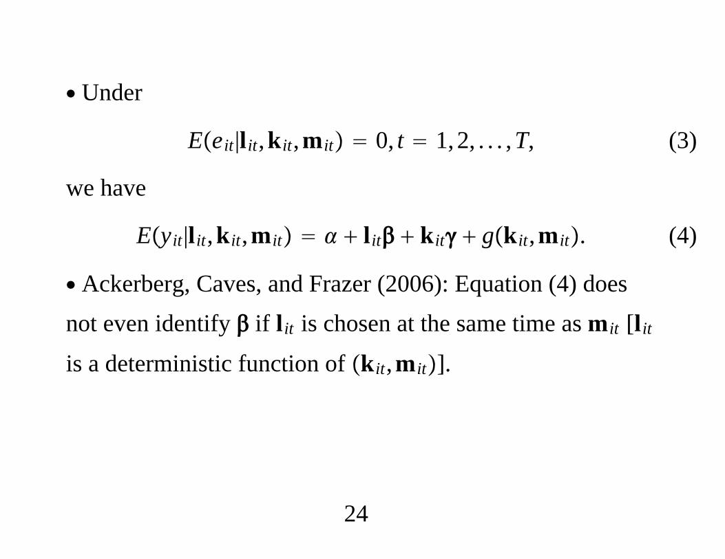
∙ Under
Eeit|lit,kit,mit 0, t 1, 2, . . . ,T, (3)
we have
Eyit|lit,kit,mit lit kit gkit,mit. (4)
∙ Ackerberg, Caves, and Frazer (2006): Equation (4) doesnot even identify if lit is chosen at the same time as mit [lit
is a deterministic function of kit,mit].
24
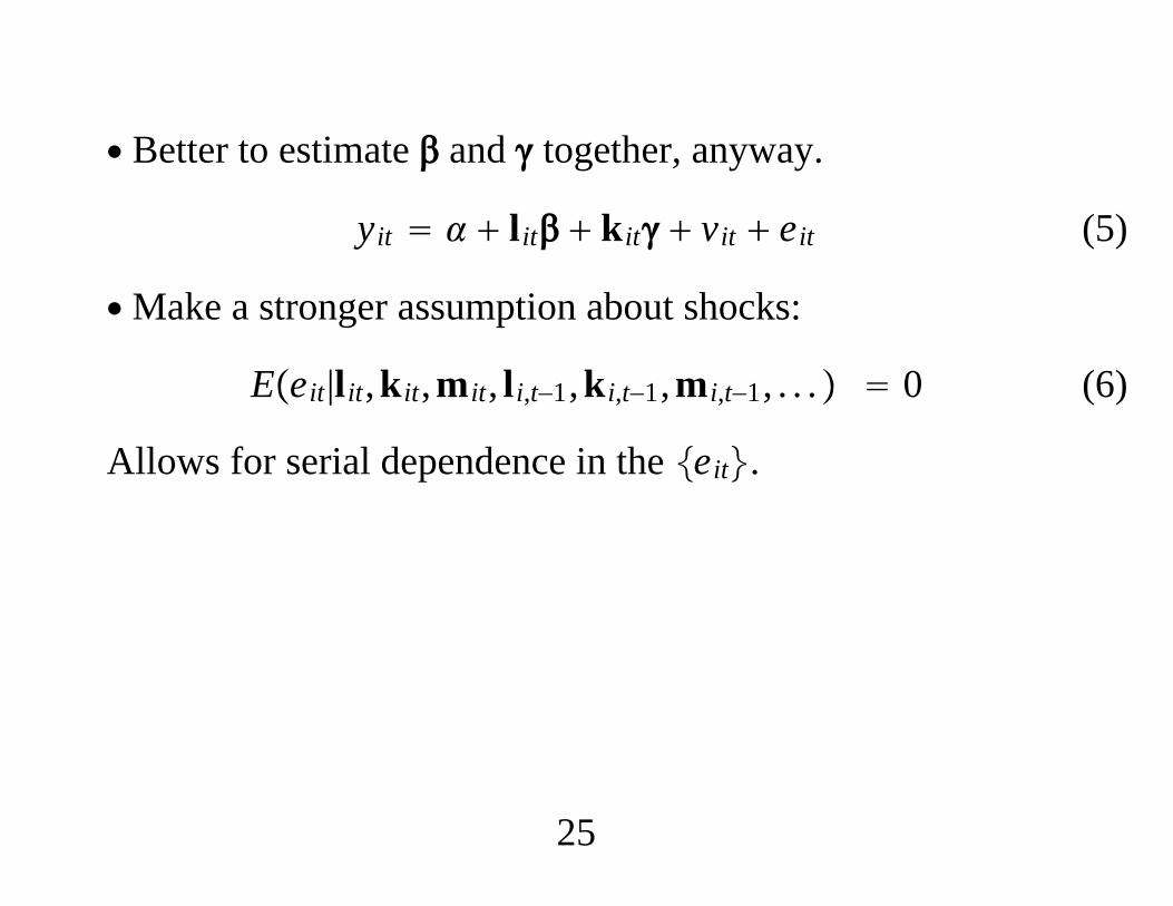
∙ Better to estimate and together, anyway.
yit lit kit vit eit (5)
∙Make a stronger assumption about shocks:
Eeit|lit,kit,mit, li,t−1,ki,t−1,mi,t−1, . . . 0 (6)
Allows for serial dependence in the eit.
25
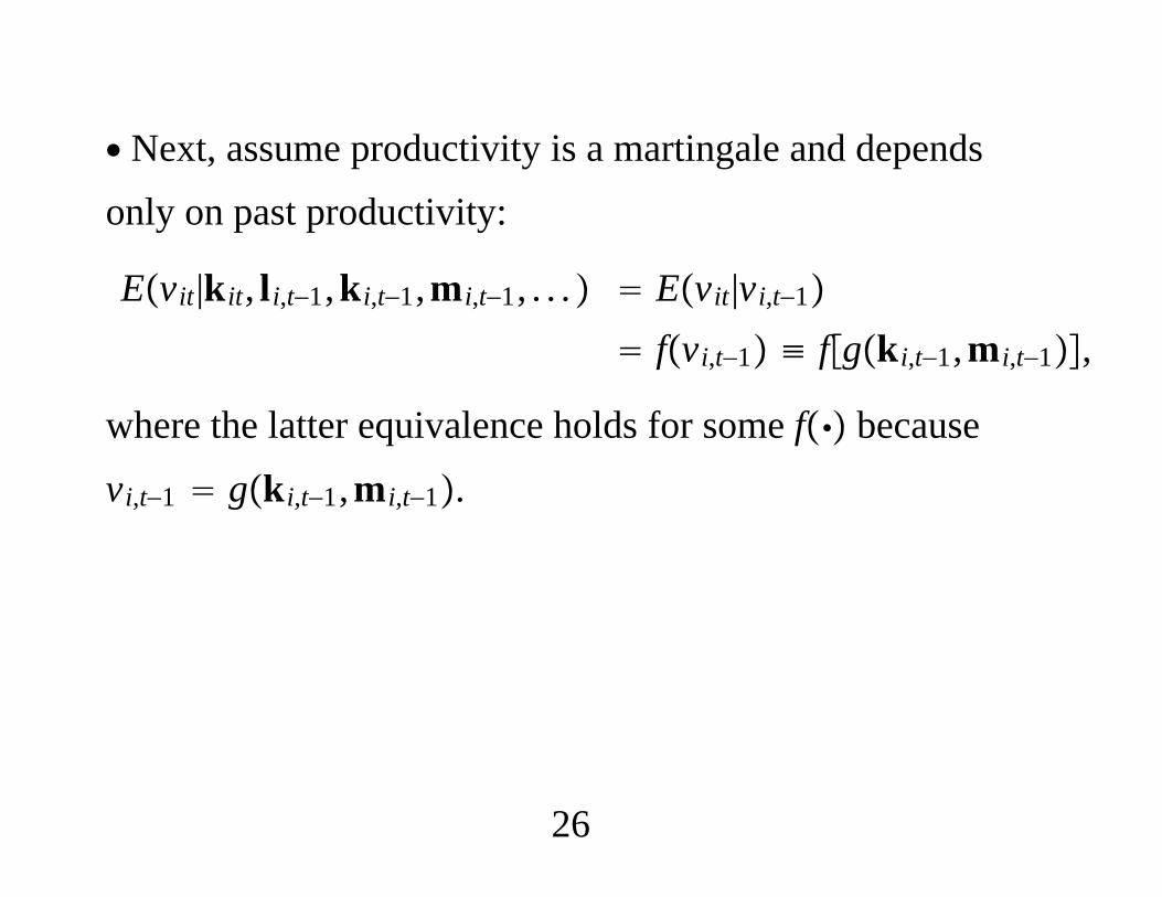
∙ Next, assume productivity is a martingale and dependsonly on past productivity:
Evit|kit, li,t−1,ki,t−1,mi,t−1, . . . Evit|vi,t−1
fvi,t−1 ≡ fgki,t−1,mi,t−1,
where the latter equivalence holds for some f becausevi,t−1 gki,t−1,mi,t−1.
26
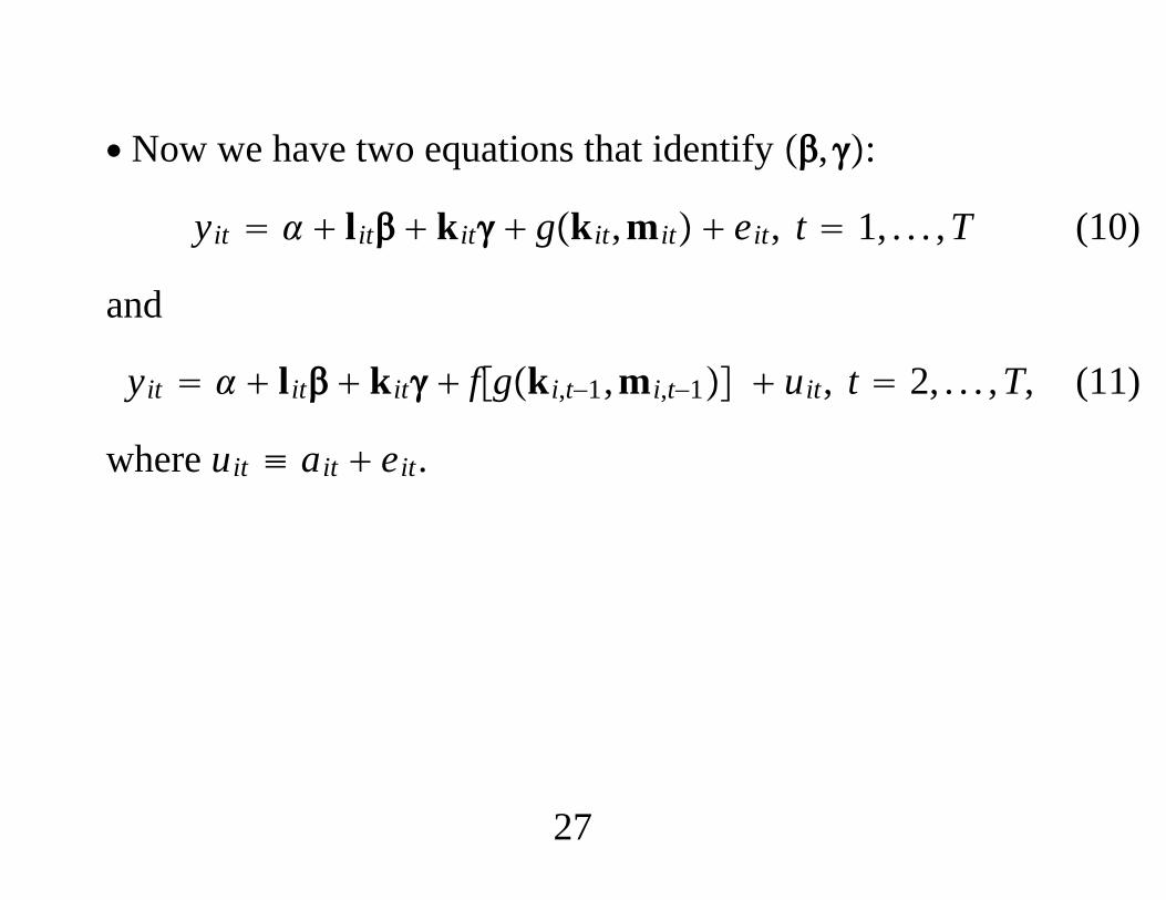
∙ Now we have two equations that identify ,:
yit lit kit gkit,mit eit, t 1, . . . ,T (10)
and
yit lit kit fgki,t−1,mi,t−1 uit, t 2, . . . ,T, (11)
where uit ≡ ait eit.
27
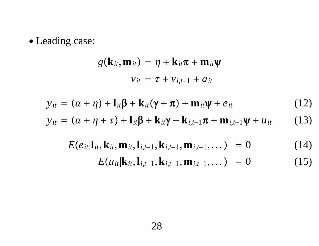
∙ Leading case:
gkit,mit kit mit
vit vi,t−1 ait
yit lit kit mit eit
yit lit kit ki,t−1 mi,t−1 uit
(12) (13)
Eeit|lit,kit,mit, li,t−1,ki,t−1,mi,t−1, . . . 0Euit|kit, li,t−1,ki,t−1,mi,t−1, . . . 0
(14) (15)
28

∙ In (12), lit, kit, and mit act as their own instruments – andthere are many extras obtained from lags of everything.∙ In (13), lit is endogenous but kit, ki,t−1, and mi,t−1 act astheir own instruments. We can use li,t−1 and other lags ofeverything as instruments for lit.
29
∙ Can use a single-equation panel data method to estimate
yit 0 lit kit ki,t−1 mi,t−1 uit (16)
∙ Could be pooled IV using instrumentsli,t−1,kit,ki,t−1,mi,t−1, pooled 2SLS with more instruments,
or efficient GMM (that accounts for serial dependence andheteroskedasticity). Petrin and Levinsohn, (2012, Rand).
30
∙ Acharya and Keller (2006, CJE) apply the two-step OPmethod and the joint GMM (OP/W) approach, and get morestable estimates of capital elasticity using the latter.∙ The labor elasticity for OP is . 548 . 054 and . 557 . 018for OP/W. For capital, the OP elasticity is . 234 . 164 forOP and the OP/W elasticity is . 513 . 105, with the OPestimate changing much more across specification.
31
3. Pseudo Panels from Pooled Cross Sections∙ Important to distinguish between the population model andthe sampling scheme. Model is
yt t xt f ut, t 1, . . . ,T,
which represents a population defined over T time periods.∙ Normalize Ef 0. Assume all elements of xt have sometime variation.∙ The current literature does not even use
Eut|xt, f 0, t 1, . . . ,T.
32
∙ Instead, we use
Eut|f 0, t 1, . . . ,T.
∙ Because f aggregates all time-constant unobservables, weare at least willing to assume
Eut|g 0
for any time-constant variable g, whether unobserved orobserved.
33
∙ Deaton (1985) considered the case of independentlysampled cross sections.∙ Assume that the population is divided into G groups (orcohorts). Common is birth year.∙ For a random draw i at time t, let gi be the group indicator,taking on a value in 1, 2, . . . ,G.
34
∙ By the previous discussion, for a random draw i,
Euit|gi 0.
∙ Taking the expected value of yt t xt f ut
conditional on group membership gives
Eyt|g t Ext|g Ef|g, t 1, . . . ,T.
∙ This is Deaton’s starting point, and Moffitt’s (1993). No“randomness” in this equation.
35

∙ Define the population means
g Ef|g, gty Eyt|g, gt
x Ext|g
for g 1, . . . ,G and t 1, . . . ,T. Then for g 1, . . . ,G andt 1, . . . ,T, we have
gty t gt
x g
∙ Important: This last equation holds without anyassumptions restricting the dependence between xt and ur
across t and r.
36
∙ xt can contain lagged dependent variables orcontemporaneously endogenous variables (due to omittedvariables, simultaneity, measurement error). Seemssuspicious.∙What is the source of identification in pseudo panels if notexogeneity restrictions?
37
∙ The equation
gty t gt
x g
looks like a linear regression model in the population cellmeans, gt
y and gtx .
∙ In the Deaton setup, with reasonable cell sizes, Ngt, treat as
a minimum distance (MD) problem.
38
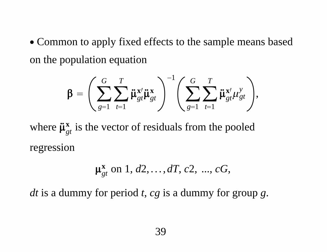
∙ Common to apply fixed effects to the sample means basedon the population equation
∑g1
G
∑t1
T
gtx′gt
x
−1
∑g1
G
∑t1
T
gtx′gt
y ,
where gtx is the vector of residuals from the pooled
regression
gtx on 1, d2, . . . ,dT, c2, ..., cG,
dt is a dummy for period t, cg is a dummy for group g.
39

∙ The population model cannot contain a full set ofgroup/time interactions.∙We would be regressing gt
x on a full set of dummy
variables dgt and then gtx 0, all g and t.
∙ If we use individual-level data we can allow forunrestricted group time effects.∙ The absense of a full cohort/time effects in the populationmodel is a key identifying restriction.
40
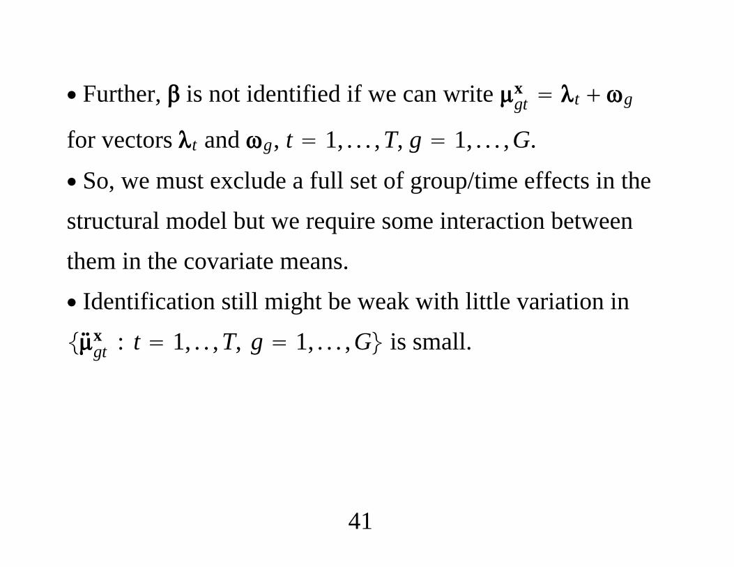
∙ Further, is not identified if we can write gtx t g
for vectors t and g, t 1, . . . ,T, g 1, . . . ,G.
∙ So, we must exclude a full set of group/time effects in thestructural model but we require some interaction betweenthem in the covariate means.∙ Identification still might be weak with little variation ingt
x : t 1, . . ,T, g 1, . . . ,G is small.
41
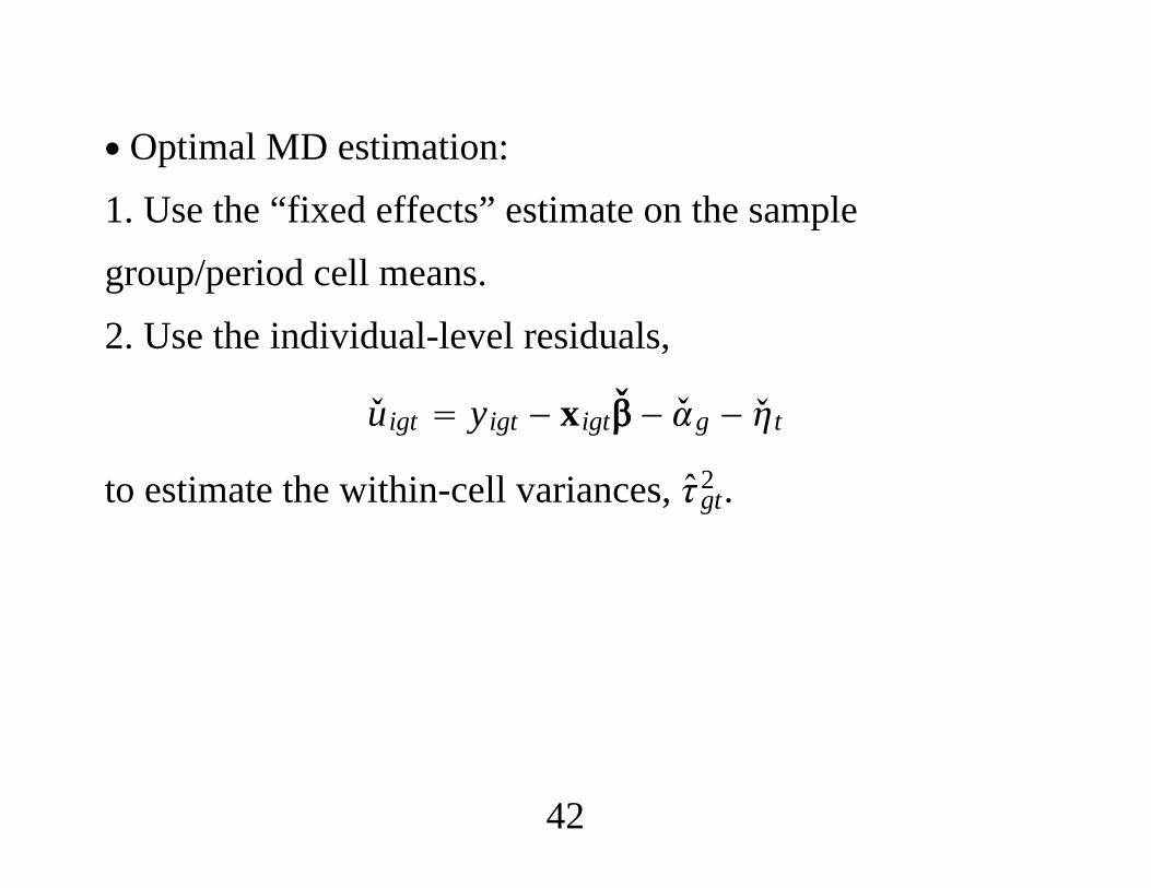
∙ Optimal MD estimation:1. Use the “fixed effects” estimate on the samplegroup/period cell means.2. Use the individual-level residuals,
u igt yigt − xigt − g − t
to estimate the within-cell variances, gt2 .
42
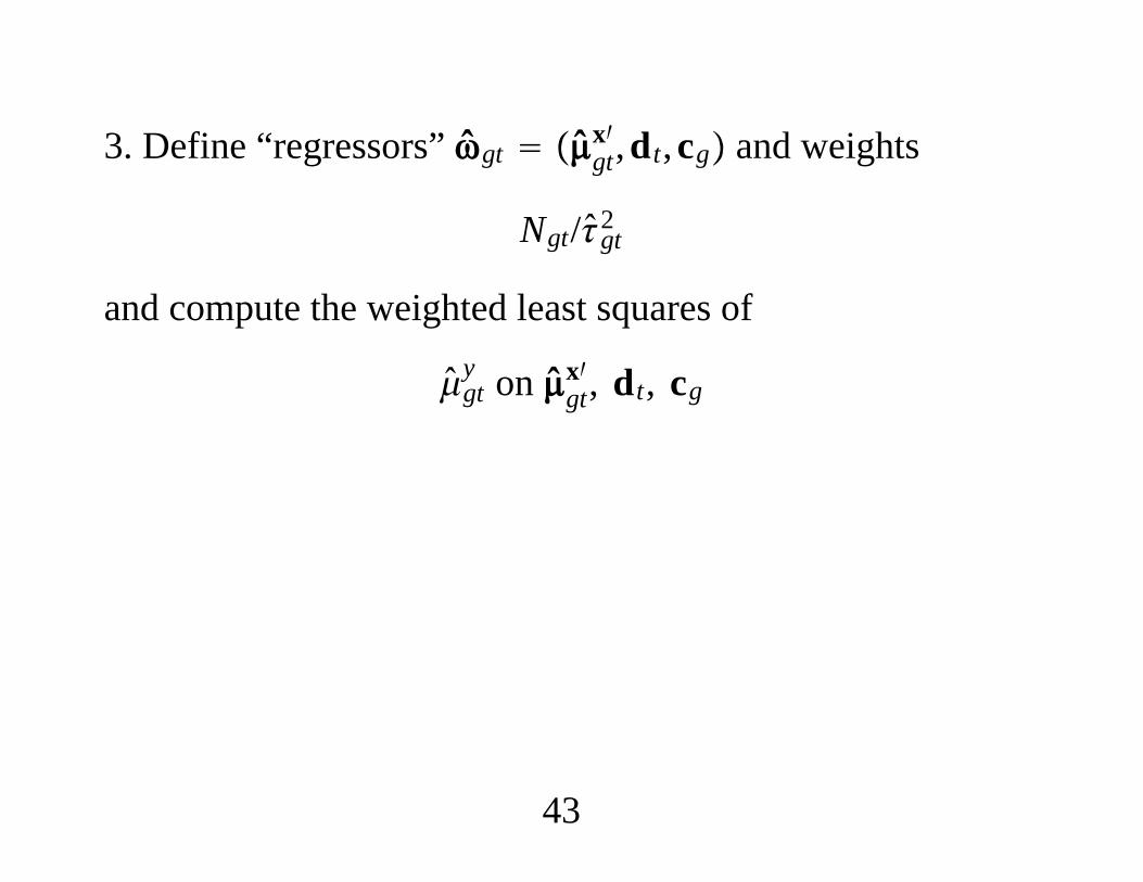
3. Define “regressors” gt gtx′,dt,cg and weights
Ngt/gt2
and compute the weighted least squares of
gty on gt
x′, dt, cg
43
∙ The asymptotic variance is estimated as the usual“weighted least squares” variance matrix.∙ GTK 1 − K T G − 1 overidentification conditions.The sum of squared residuals from the weighted leastsquares regression is distributed as GTK1−KTG−1
2 if the
restrictions are true.
44
∙ Deaton (1985), VN (1993), and Collado (1998), use adifferent asymptotic analysis: GT → with fixed cell sizes.∙ Some authors try to have it both ways (first ignoring theestimation error in the cell means, so Ngt is large, and then
assuming a large number of groups and/or time periods).∙ Open question: If one just wants to use the “fixed effects”estimator, and not use the individual-level data, how can oneperform valid inference?
45

"Econometrics of Cross Section and Panel Data"
Lecture 5
Instrumental Variables
Guido Imbens
Cemmap Lectures, UCL, June 2014

Outline
1. Introduction
2. Linear Instrumental Variables with Constant Coefficients
3. Potential Outcomes
4. Local Average Treatment Effects
5. Effects of Military Service on Earnings
6. Multivalued Instruments
1

7. Multivalued Endogenous Variables
8. Instrumental Variables Estimates of the Returns to Educa-
tion Using Quarter of Birth as an Instrument
1. Introduction
Here we investigate the interpretation of instrumental variables
estimators allowing for general heterogeneity in the effect of
the endogenous regressor.
The general theme is that with heterogenous effects endo-
geneity creates severe problems for identification of population
parameters. In general we can only identify average effects for
subpopulations that are induced by the instrument to change
the value of the endogenous regressors. We refer to such sub-
populations as compliers.
These complier subpopulations are not always the subpopu-
lations that are ex ante the most interesting subpopulations,
but there the data may just not be informative about average
effects for other subpopulations without extrapolation.
2
2. Linear Instrumental Variables with Constant Coeffi-
cients
In the example we are interested in the causal effect of military
service on earnings. Let Yi be the outcome for unit i, Wi the
endogenous regressor, and Zi the instrument. A linear model
is postulated for the relation between the outcome and the
endogenous regressor:
Yi = β0 + β1 · Wi + εi.
This is a structural/behavioral/causal relationshiup. There is
concern that the regressor Wi is endogenous, that is, that Wiis correlated with εi.
Suppose that we are confident that a second variable, the in-
strument Zi is uncorrelated with the unobserved component
and correlated with the endogenous regressor. The solution is
to use Zi as an instrument for Wi.
3

In Two-Stage-Least-Squares we first estimate a linear regres-
sion of the endogenous regressor on the instrument by least
squares. Let the estimated regression function be
Wi = α0 + α1 · Zi.
Then we regress the outcome on the predicted value of the
endogenousr regressor, using least squares:
Yi = β0 + βTSLS1 · Wi.
4
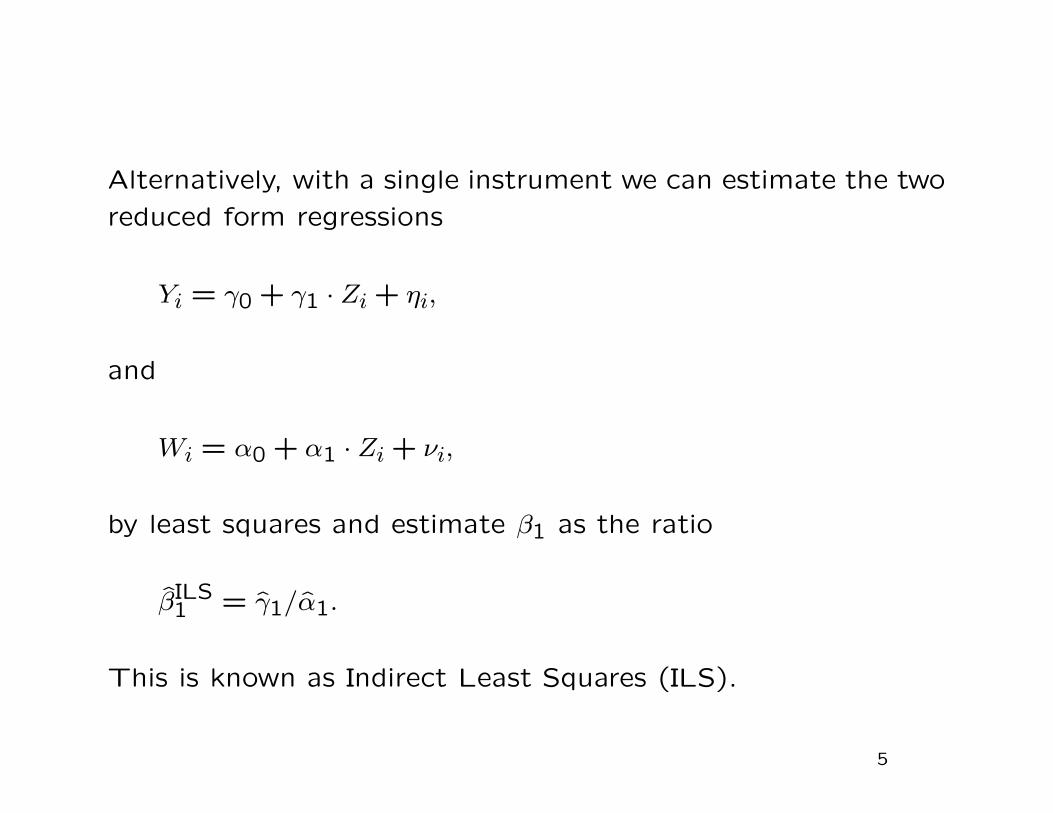
Alternatively, with a single instrument we can estimate the two
reduced form regressions
Yi = γ0 + γ1 · Zi + ηi,
and
Wi = α0 + α1 · Zi + νi,
by least squares and estimate β1 as the ratio
βILS1 = γ1/α1.
This is known as Indirect Least Squares (ILS).
5

If there is a single instrument and single endogenous regressor,
we end up in both cases with the ratio of the sample covariance
of Y and Z to the sample covariance of W and Z.
β1 = βTSLS1 = βILS
1 =1N
∑Ni=1(Yi − Y ) · (Zi − Z)
1N
∑Ni=1(Wi − W ) · (Zi − Z)
.
Using a central limit theorem for all the moments and the
delta method we can infer the large sample distribution without
additional assumptions.
With multiple instruments TSLS and ILS generally differ. (There
are multiple ratios that can be used in the ILS derivation.)
6
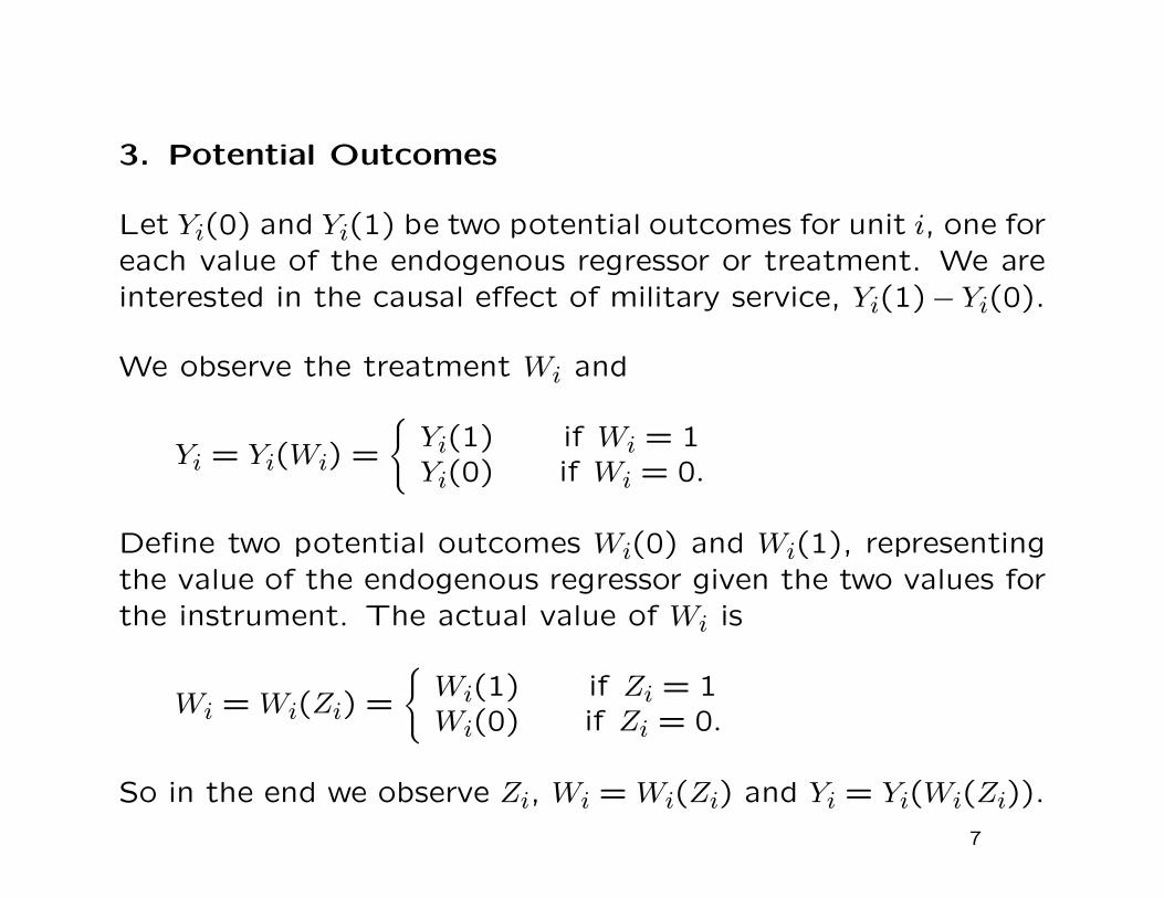
3. Potential Outcomes
Let Yi(0) and Yi(1) be two potential outcomes for unit i, one for
each value of the endogenous regressor or treatment. We are
interested in the causal effect of military service, Yi(1)− Yi(0).
We observe the treatment Wi and
Yi = Yi(Wi) =
Yi(1) if Wi = 1Yi(0) if Wi = 0.
Define two potential outcomes Wi(0) and Wi(1), representing
the value of the endogenous regressor given the two values for
the instrument. The actual value of Wi is
Wi = Wi(Zi) =
Wi(1) if Zi = 1Wi(0) if Zi = 0.
So in the end we observe Zi, Wi = Wi(Zi) and Yi = Yi(Wi(Zi)).
7
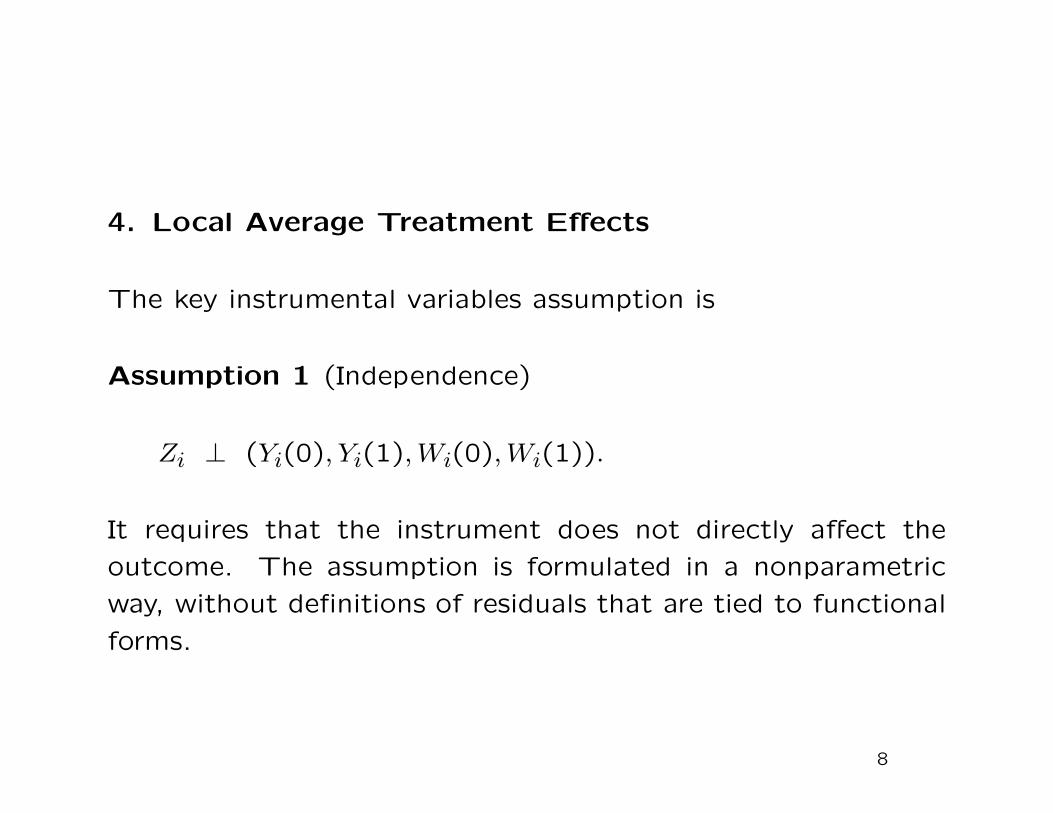
4. Local Average Treatment Effects
The key instrumental variables assumption is
Assumption 1 (Independence)
Zi ⊥ (Yi(0), Yi(1), Wi(0), Wi(1)).
It requires that the instrument does not directly affect the
outcome. The assumption is formulated in a nonparametric
way, without definitions of residuals that are tied to functional
forms.
8
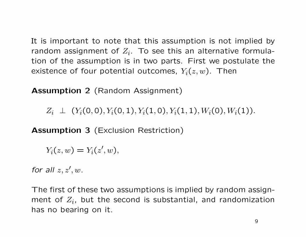
It is important to note that this assumption is not implied by
random assignment of Zi. To see this an alternative formula-
tion of the assumption is in two parts. First we postulate the
existence of four potential outcomes, Yi(z, w). Then
Assumption 2 (Random Assignment)
Zi ⊥ (Yi(0,0), Yi(0,1), Yi(1,0), Yi(1,1), Wi(0), Wi(1)).
Assumption 3 (Exclusion Restriction)
Yi(z, w) = Yi(z′, w),
for all z, z′, w.
The first of these two assumptions is implied by random assign-
ment of Zi, but the second is substantial, and randomization
has no bearing on it.
9
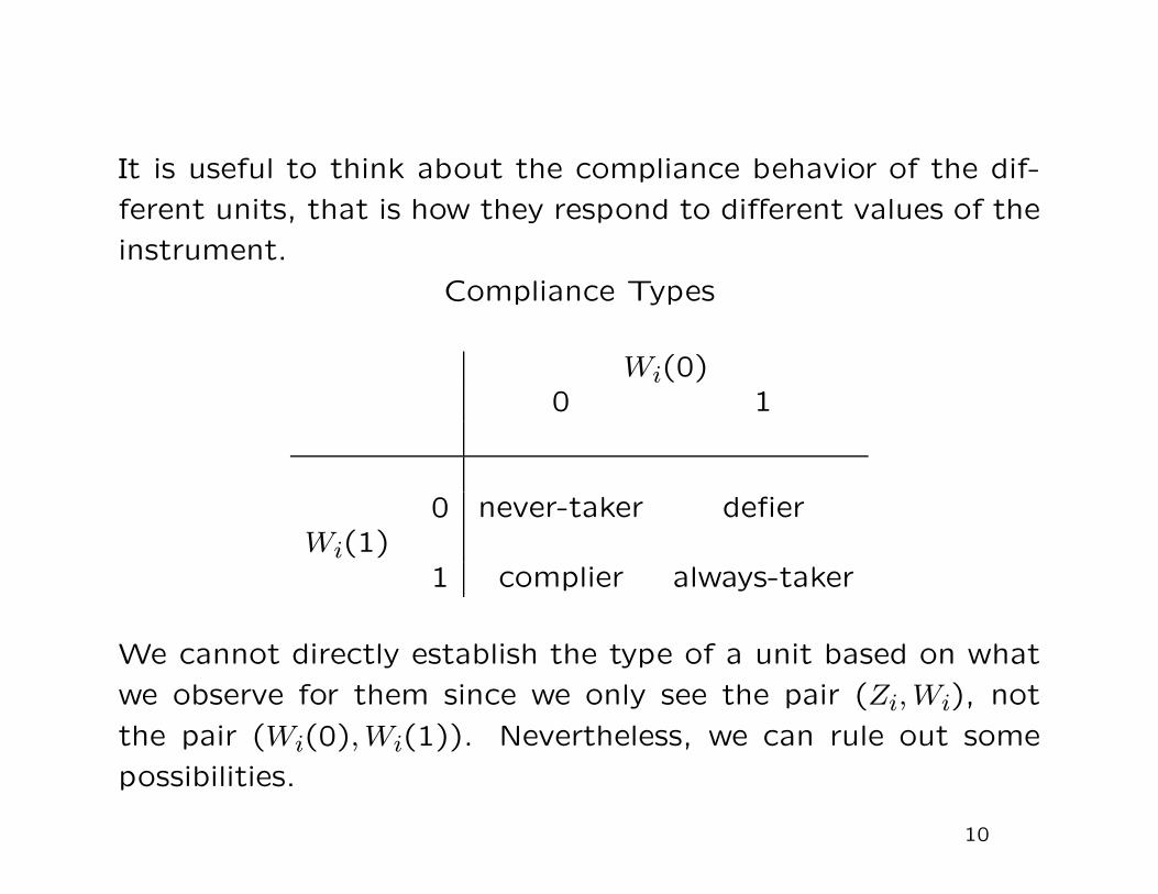
It is useful to think about the compliance behavior of the dif-
ferent units, that is how they respond to different values of the
instrument.
Compliance Types
Wi(0)0 1
0 never-taker defierWi(1)
1 complier always-taker
We cannot directly establish the type of a unit based on what
we observe for them since we only see the pair (Zi, Wi), not
the pair (Wi(0), Wi(1)). Nevertheless, we can rule out some
possibilities.
10
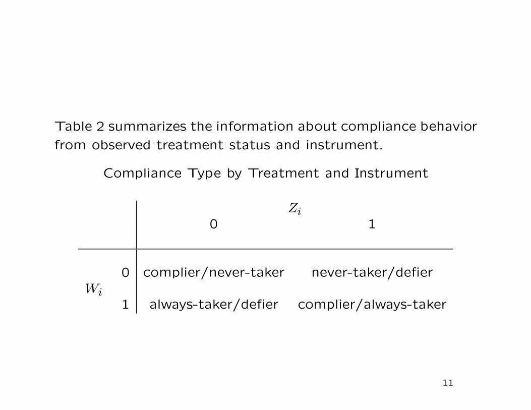
Table 2 summarizes the information about compliance behavior
from observed treatment status and instrument.
Compliance Type by Treatment and Instrument
Zi0 1
0 complier/never-taker never-taker/defierWi
1 always-taker/defier complier/always-taker
11
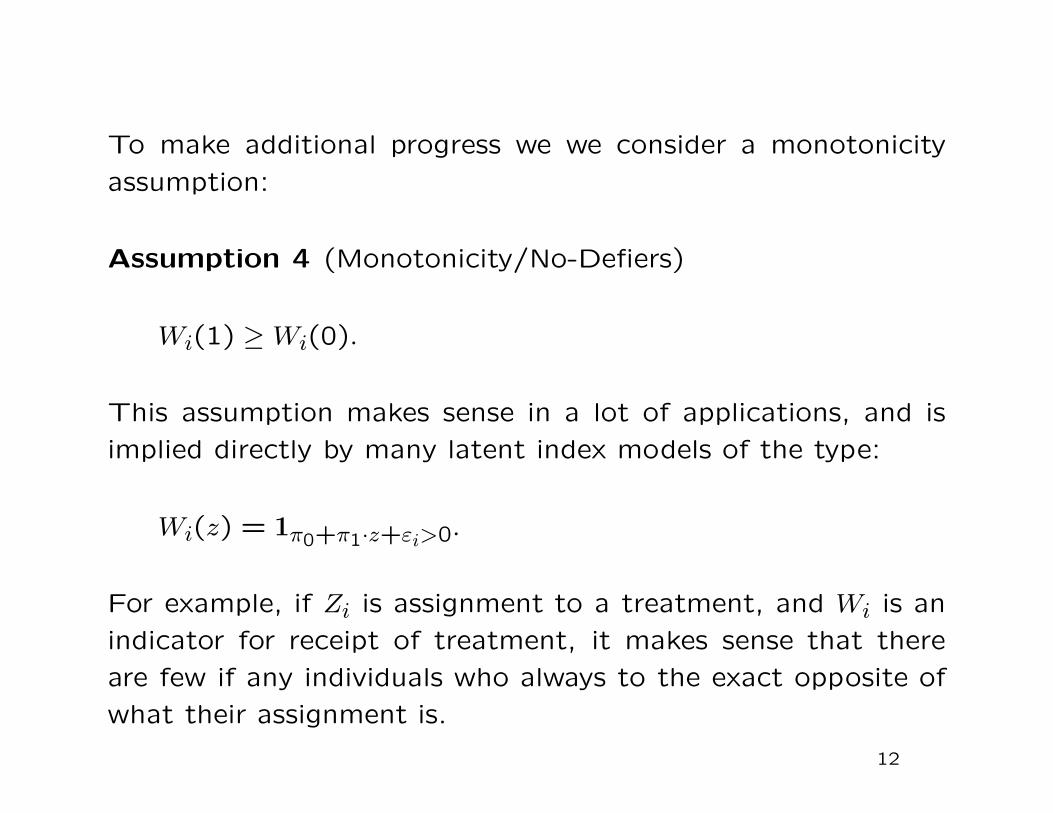
To make additional progress we we consider a monotonicity
assumption:
Assumption 4 (Monotonicity/No-Defiers)
Wi(1) ≥ Wi(0).
This assumption makes sense in a lot of applications, and is
implied directly by many latent index models of the type:
Wi(z) = 1π0+π1·z+εi>0.
For example, if Zi is assignment to a treatment, and Wi is an
indicator for receipt of treatment, it makes sense that there
are few if any individuals who always to the exact opposite of
what their assignment is.
12
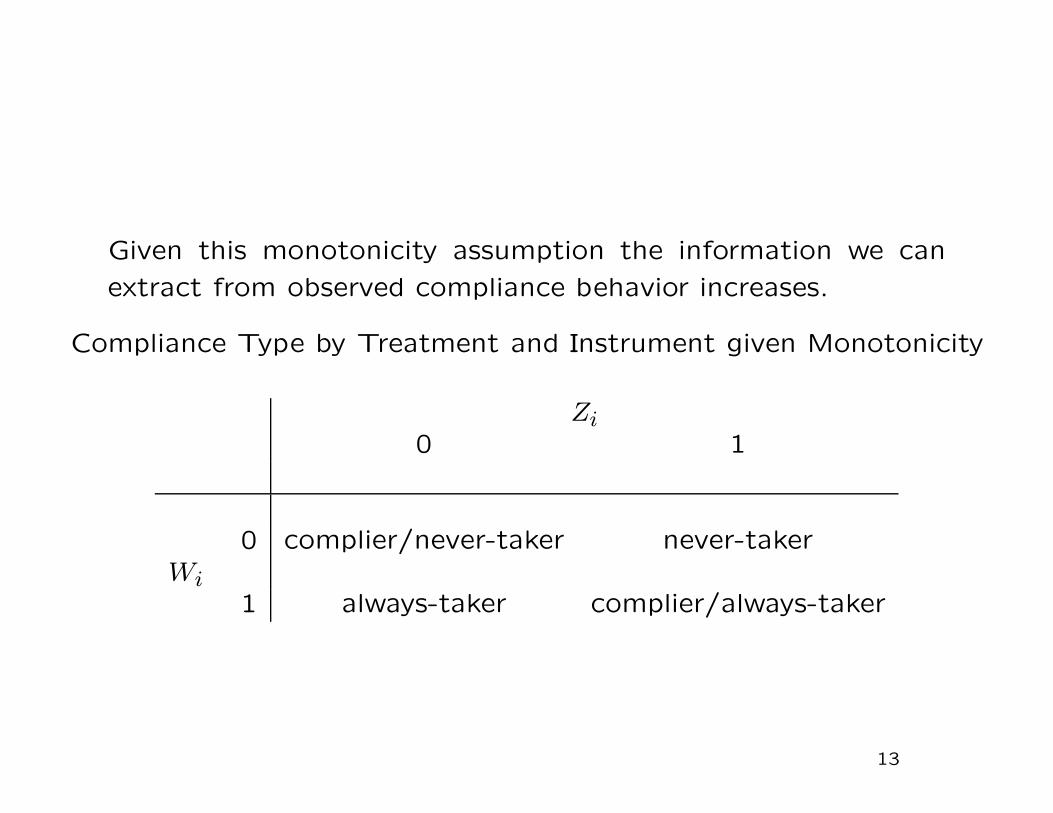
Given this monotonicity assumption the information we can
extract from observed compliance behavior increases.
Compliance Type by Treatment and Instrument given Monotonicity
Zi0 1
0 complier/never-taker never-takerWi
1 always-taker complier/always-taker
13
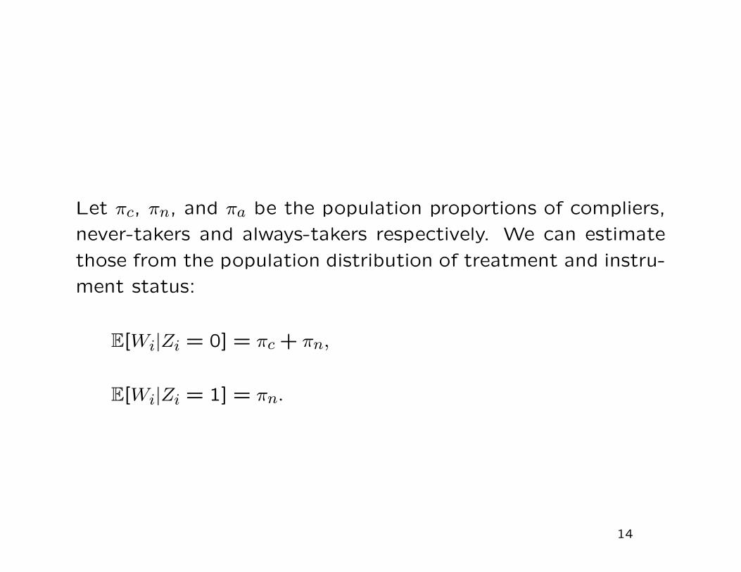
Let πc, πn, and πa be the population proportions of compliers,
never-takers and always-takers respectively. We can estimate
those from the population distribution of treatment and instru-
ment status:
E[Wi|Zi = 0] = πc + πn,
E[Wi|Zi = 1] = πn.
14
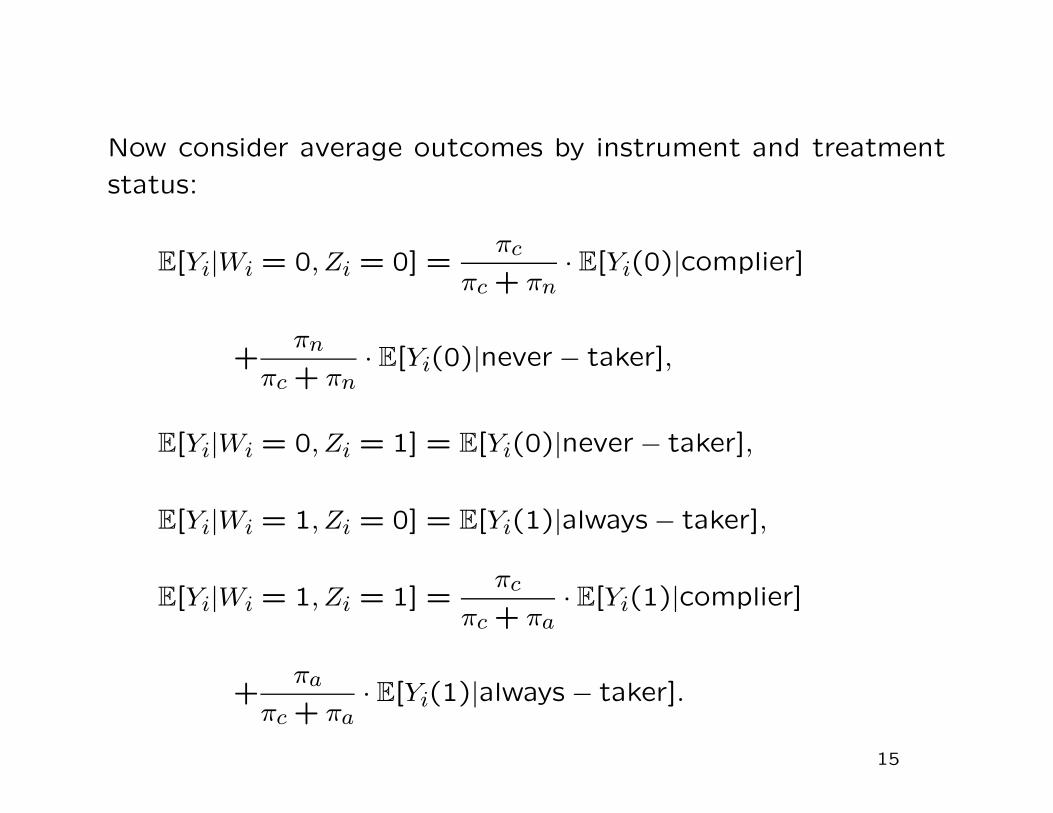
Now consider average outcomes by instrument and treatment
status:
E[Yi|Wi = 0, Zi = 0] =πc
πc + πn· E[Yi(0)|complier]
+πn
πc + πn· E[Yi(0)|never − taker],
E[Yi|Wi = 0, Zi = 1] = E[Yi(0)|never − taker],
E[Yi|Wi = 1, Zi = 0] = E[Yi(1)|always − taker],
E[Yi|Wi = 1, Zi = 1] =πc
πc + πa· E[Yi(1)|complier]
+πa
πc + πa· E[Yi(1)|always − taker].
15
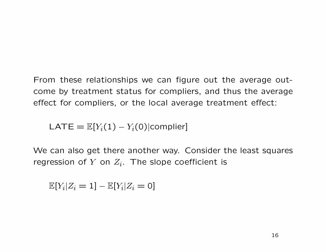
From these relationships we can figure out the average out-
come by treatment status for compliers, and thus the average
effect for compliers, or the local average treatment effect:
LATE = E[Yi(1)− Yi(0)|complier]
We can also get there another way. Consider the least squares
regression of Y on Zi. The slope coefficient is
E[Yi|Zi = 1] − E[Yi|Zi = 0]
16

Consider the first term:
E[Yi|Zi = 1] = E[Yi|Zi = 1, complier] · Pr(complier|Zi = 1)
+E[Yi|Zi = 1,never − taker] · Pr(never − taker|Zi = 1)
+E[Yi|Zi = 1,always− taker] · Pr(always − taker|Z = 1)
= E[Yi(1)|complier] · πc
+E[Yi(0)|never − taker] · πn + E[Yi(1)|always − taker] · πa.
17
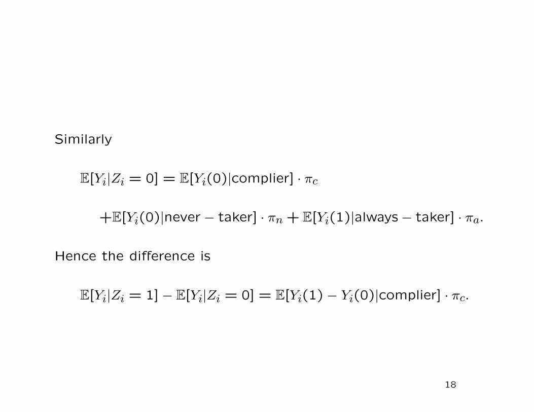
Similarly
E[Yi|Zi = 0] = E[Yi(0)|complier] · πc
+E[Yi(0)|never − taker] · πn + E[Yi(1)|always − taker] · πa.
Hence the difference is
E[Yi|Zi = 1] − E[Yi|Zi = 0] = E[Yi(1) − Yi(0)|complier] · πc.
18
The same argument can be used to show that the slope coef-
ficient in the regression of Wi on Zi is
E[Wi|Zi = 1] = E[Wi|Zi = 0] = πc.
Hence the instrumental variables estimand is the ratio, equal
to the local average treatment effect E[Yi(1)−Yi(0)|complier].
The key insight is that the data are informative about the
average effect for compliers only. Put differently, the data
are not informative about the average effect for nevertakers
because they are never seen receiving the treatment, and they
are not informative about the average effect for alwaystakers
because they are never seen without the treatment.
19

5. Effects of Military Service on Earnings
Angrist (1989) was interested in estimating the effect of serving
in the military on earnings. There is obvious concern about the
fact that those choosing to serve in the military are likely to
be different from those who dont. Which way do you expect
the bias to go?
To avoid such biases he exploited the Vietnam era draft lottery.
Specifically he uses the binary indicator whether or not your
draft lottery number made you eligible to be drafted as an
instrument.
This was tied to your day of birth, so more or less random.
Even so, that does not make it valid as an instrument. What
are potential reasons for this instrument not to be valid?
As the outcome of interest we take log earnings.
20

The simple ols regression leads to:
log(earnings)i = 5.4364 − 0.0205 · veterani
(0079) (0.0167)
21
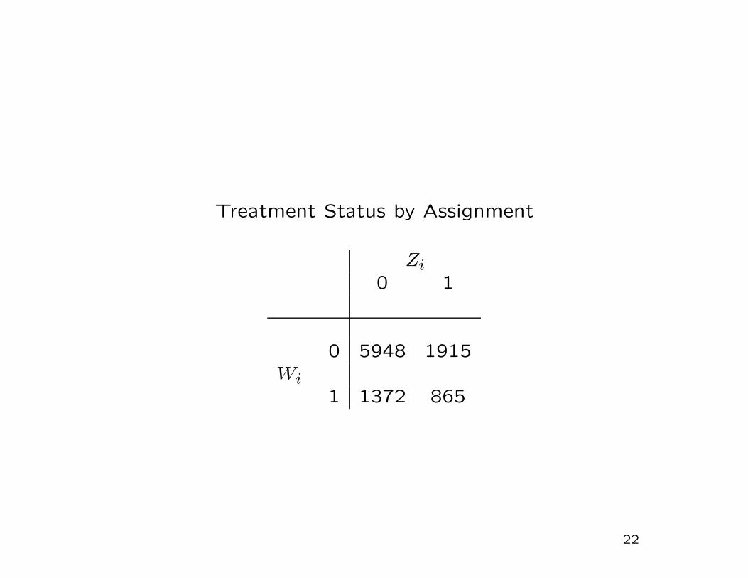
Treatment Status by Assignment
Zi0 1
0 5948 1915Wi
1 1372 865
22
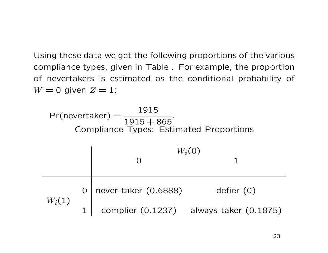
Using these data we get the following proportions of the various
compliance types, given in Table . For example, the proportion
of nevertakers is estimated as the conditional probability of
W = 0 given Z = 1:
Pr(nevertaker) =1915
1915 + 865.
Compliance Types: Estimated Proportions
Wi(0)0 1
0 never-taker (0.6888) defier (0)Wi(1)
1 complier (0.1237) always-taker (0.1875)
23

Table gives the average outcomes for the four groups, by
treatment and instrument status.
Estimated Average Outcomes by Treatment and Instrument
Zi0 1
0 E[Yi] = 5.4472 E[Yi] = 5.4028Wi
1 E[Yi] = 5.4076, E[Yi] = 5.4289
24
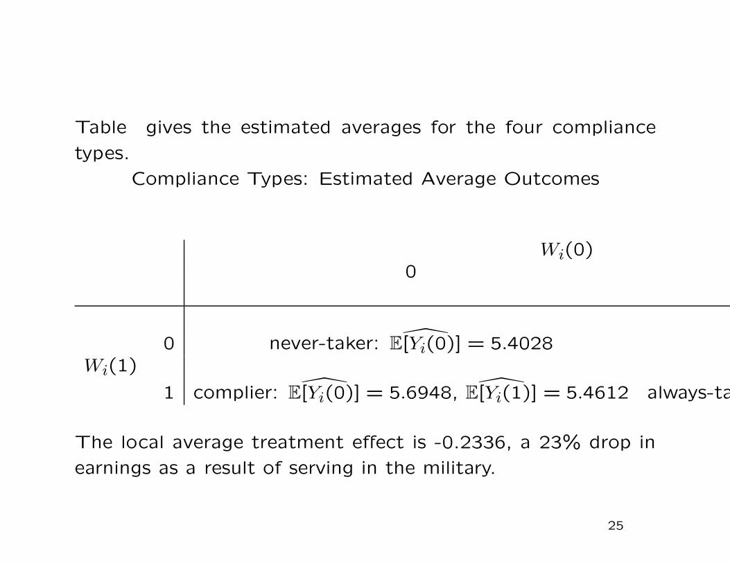
Table gives the estimated averages for the four compliance
types.
Compliance Types: Estimated Average Outcomes
Wi(0)0
0 never-taker: E[Yi(0)] = 5.4028Wi(1)
1 complier: E[Yi(0)] = 5.6948, E[Yi(1)] = 5.4612 always-tak
The local average treatment effect is -0.2336, a 23% drop in
earnings as a result of serving in the military.
25
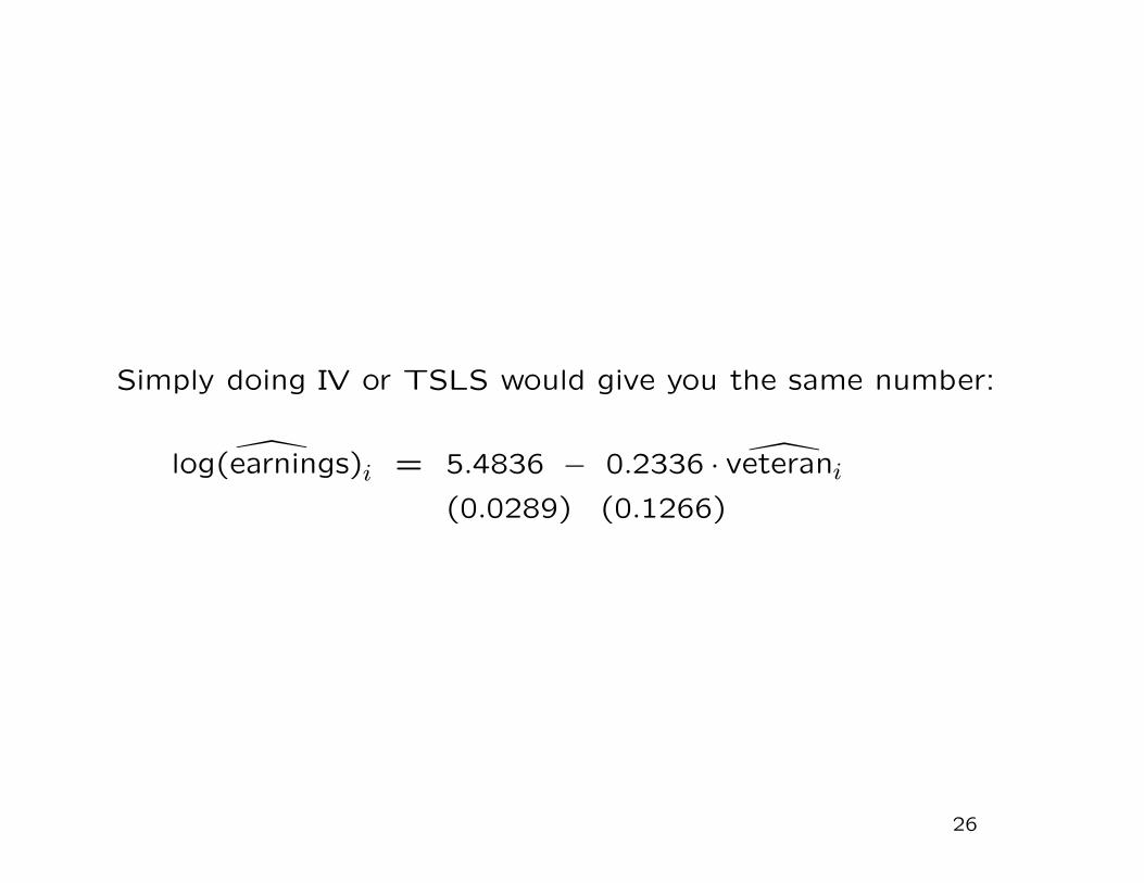
Simply doing IV or TSLS would give you the same number:
log(earnings)i = 5.4836 − 0.2336 · veterani
(0.0289) (0.1266)
26
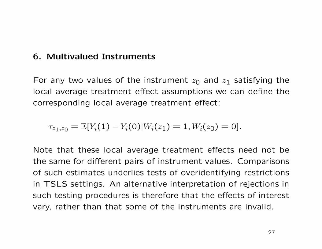
6. Multivalued Instruments
For any two values of the instrument z0 and z1 satisfying the
local average treatment effect assumptions we can define the
corresponding local average treatment effect:
τz1,z0 = E[Yi(1) − Yi(0)|Wi(z1) = 1, Wi(z0) = 0].
Note that these local average treatment effects need not be
the same for different pairs of instrument values. Comparisons
of such estimates underlies tests of overidentifying restrictions
in TSLS settings. An alternative interpretation of rejections in
such testing procedures is therefore that the effects of interest
vary, rather than that some of the instruments are invalid.
27

Suppose that we have an instrument Zi with support z0, z1, . . . , zK,
ordered in such a way that
p(zk−1) ≤ p(zk),
where
p(z) = E[Wi|Zi = z].
This is like a monotonicity assumption.
Also suppose that the instrument is relevant,
E[g(Zi) · Wi] 6= 0.
28
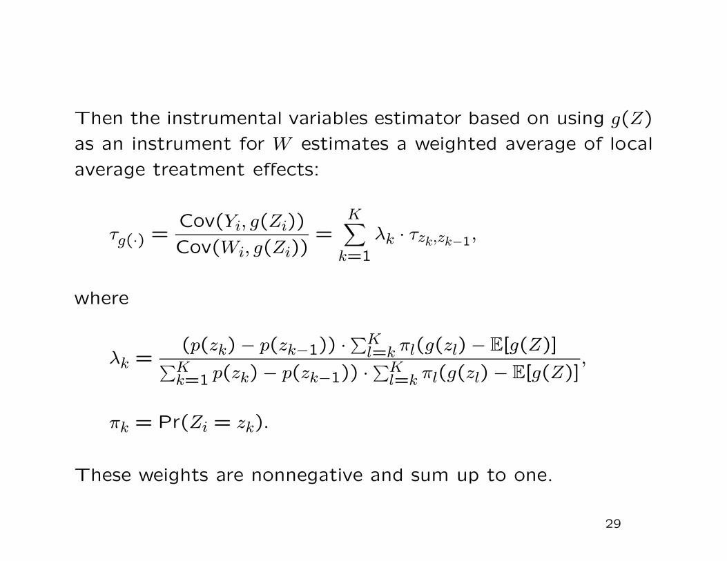
Then the instrumental variables estimator based on using g(Z)
as an instrument for W estimates a weighted average of local
average treatment effects:
τg(·) =Cov(Yi, g(Zi))
Cov(Wi, g(Zi))=
K∑
k=1
λk · τzk,zk−1,
where
λk =(p(zk) − p(zk−1)) ·
∑Kl=k πl(g(zl) − E[g(Z)]
∑Kk=1 p(zk) − p(zk−1)) ·
∑Kl=k πl(g(zl) − E[g(Z)]
,
πk = Pr(Zi = zk).
These weights are nonnegative and sum up to one.
29
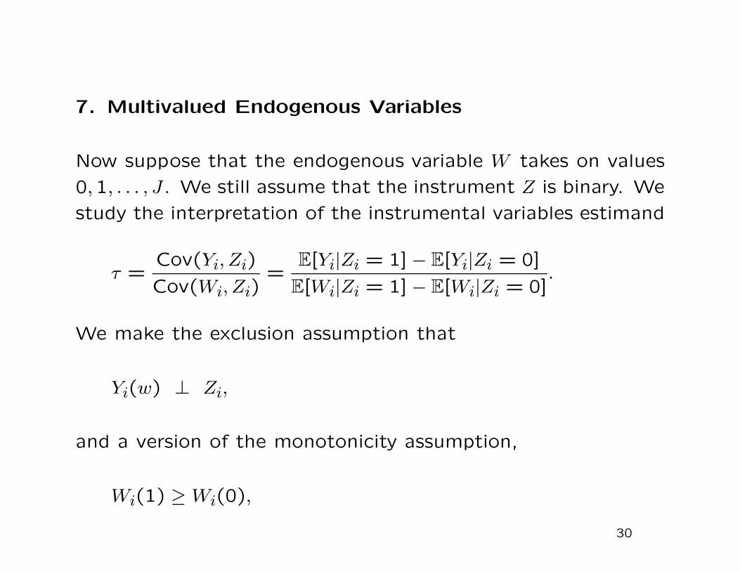
7. Multivalued Endogenous Variables
Now suppose that the endogenous variable W takes on values
0,1, . . . , J. We still assume that the instrument Z is binary. We
study the interpretation of the instrumental variables estimand
τ =Cov(Yi, Zi)
Cov(Wi, Zi)=
E[Yi|Zi = 1] − E[Yi|Zi = 0]
E[Wi|Zi = 1] − E[Wi|Zi = 0].
We make the exclusion assumption that
Yi(w) ⊥ Zi,
and a version of the monotonicity assumption,
Wi(1) ≥ Wi(0),
30

Then we can write the instrumental variables estimand as
τ =J∑
j=1
λj · E[Yi(j)− Yi(j − 1)|Wi(1) ≥ j > Wi(0)],
where
λj =Pr(Wi(1) ≥ j > Wi(0)
∑Ji=1 Pr(Wi(1) ≥ i > Wi(0)
.
31

Note that we can estimate the weights λj because
Pr(Wi(1) ≥ j > Wi(0) = Pr(Wi(1) ≥ j)− Pr(Wi(0) ≥ j)
= Pr(Wi(1) ≥ j|Zi = 1)− Pr(Wi(0) ≥ j|Zi = 0)
= Pr(Wi ≥ j|Zi = 1)− Pr(Wi ≥ j|Zi = 0).
32

8. Instrumental Variables Estimates of the Returns to
Education Using Quarter of Birth as an Instrument
Here we use a subset of the data used by Angrist and Krueger
in their 1991 study of the returns to education.
Their idea was that individuals born in different parts of the
year are subject to slightly different compulsory schooling laws.
Angrist and Krueger implement this using census data with
quarter of birth indicators as the instrument.
33

Average Level of Education by Quarter of Birth
quarter 1 2 3 4
average level of education 12.69 12.74 12.81 12.84
standard error 0.01 0.01 0.01 0.01
number of observations 81,671 80,138 86,856 80,844
34

In the illustrations below we just use a single instrument, an
indicator for being born in the first quarter. First let us look
at the reduced form regressions of log earnings and years of
education on the first quarter of birth dummy:
educi = 12.797 − 0.109 · educi
(0.006) (0.013)
and
log(earnings)i = 5.903 − 0.011 · educi
(0.001) (0.003)
The instrumental variables estimate is the ratio of the reduced
form coefficients,
βIV =−0.1019
−0.011= 0.1020.
35

Now let us interpret this in the context of heterogeneous re-
turns to education.
This estimate is an average of returns to education, consisting
of two types of averaging.
The first is over different levels of education.
In addition, for any level, e.g., to moving from nine to ten
years of education, it is an average effect where the averag-
ing is over those people whose schooling would have been at
least ten years of education if the compulsory schooling laws
had been those effective for individuals born in the second to
fourth quarter, and who would have had less than ten years of
education had they been subject to the compulsory schooling
laws in effect for individuals born in the first quarter.
36
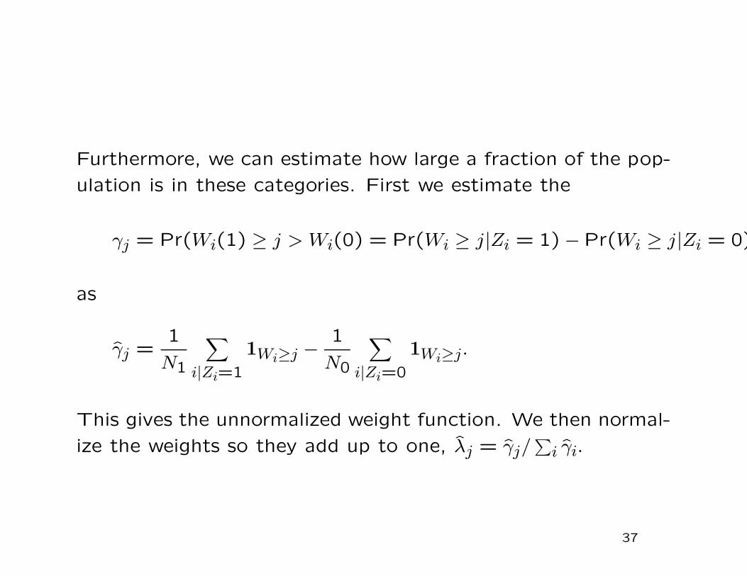
Furthermore, we can estimate how large a fraction of the pop-
ulation is in these categories. First we estimate the
γj = Pr(Wi(1) ≥ j > Wi(0) = Pr(Wi ≥ j|Zi = 1) −Pr(Wi ≥ j|Zi = 0)
as
γj =1
N1
∑
i|Zi=1
1Wi≥j −1
N0
∑
i|Zi=0
1Wi≥j.
This gives the unnormalized weight function. We then normal-
ize the weights so they add up to one, λj = γj/∑
i γi.
37

Econometrics of Cross Section and Panel DataLecture 6: Nonlinear Panel Data Models
Jeff WooldridgeMichigan State University
cemmap/PEPA, June 2014
1. Linear versus Nonlinear Models2. Quantities of Interest: Average Partial Effects3. Assumptions for Nonlinear Models4. Binary/Fractional Response Models5. Exponential Models6. Dynamic Models
1
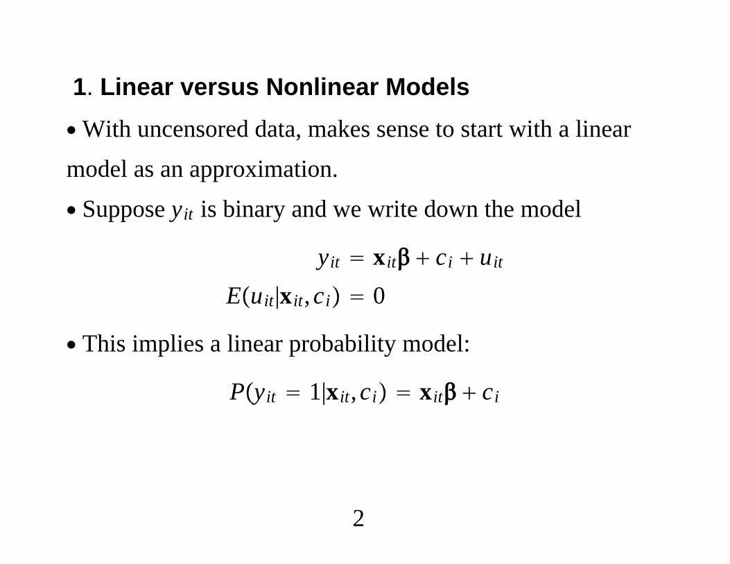
1. Linear versus Nonlinear Models∙With uncensored data, makes sense to start with a linearmodel as an approximation.∙ Suppose yit is binary and we write down the model
yit xit ci uit
Euit|xit,ci 0
∙ This implies a linear probability model:
Pyit 1|xit,ci xit ci
2
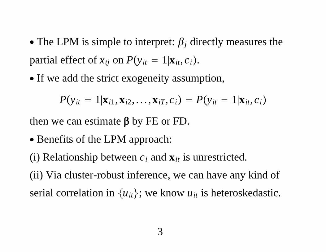
∙ The LPM is simple to interpret: j directly measures the
partial effect of xtj on Pyit 1|xit,ci.
∙ If we add the strict exogeneity assumption,
Pyit 1|xi1,xi2, . . . ,xiT,ci Pyit 1|xit,ci
then we can estimate by FE or FD.
∙ Benefits of the LPM approach:(i) Relationship between ci and xit is unrestricted.(ii) Via cluster-robust inference, we can have any kind ofserial correlation in uit; we know uit is heteroskedastic.
3
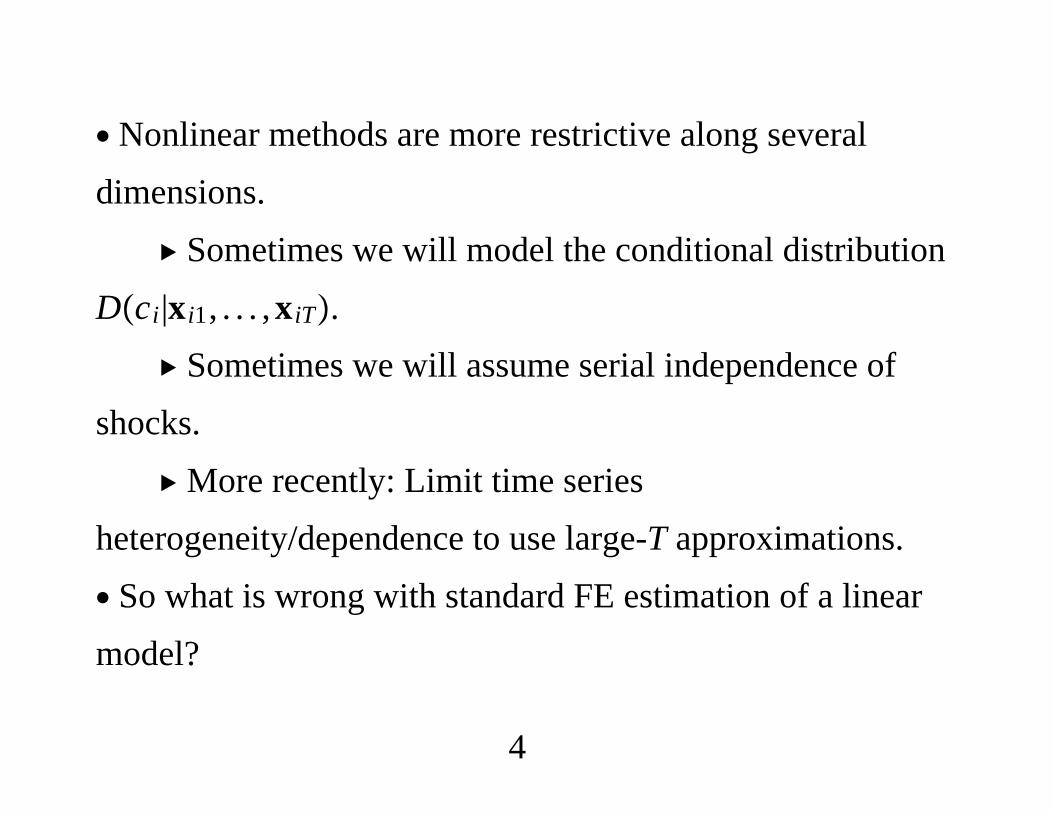
∙ Nonlinear methods are more restrictive along severaldimensions.
Sometimes we will model the conditional distributionDci|xi1, . . . ,xiT.
Sometimes we will assume serial independence ofshocks.
More recently: Limit time seriesheterogeneity/dependence to use large-T approximations.∙ So what is wrong with standard FE estimation of a linearmodel?
4
∙ Answer: The linear functional form for Pyit 1|xit,ci
cannot hold over a wide range of values for xit and ci.∙ If we take the LPM literally, we must have
0 ≤ xit ci ≤ 1, all xit,
which puts strange restrictions on the heterogeneitydistribution.∙ Should view the LPM as a linear approximation. FEestimates of the j can give reasonable estimates of average
marginal effects.
5
2. Quantities of Interest: Average Partial Effects∙ Start with the unobserved effects probit model:
Pyit 1|xit,ci xit ci, t 1, . . . ,T
where is the standard normal cdf∙ Logit replaces z with
z expz/1 expz.
6
∙What are the quantities of interest? Parameters, but alsopartial effects.∙ For a continuous xtj, the PE is
∂Pyt 1|xt,c∂xtj
jxt c,
where is the standard normal pdf.
∙ The PE depends on xt and c.∙ The sign of the PE is the same as the sign of j, but we
usually want a magnitude.
7
∙ If we have two continuous variables, the ratio of the partialeffects is constant and equal to the ratio of coefficients:
jxt chxt c
jh
But this still does not tell us the size of each effect.
8

∙ General Setup: Suppose we are interested in
Eyit|xit,ci mtxit,ci,
where ci can be a vector of unobserved heterogeneity.∙ Partial effects: If xtj is continuous, then its PE is
jxt,c ≡∂mtxt,c∂xtj
.
∙ Issues for discrete changes are similar.
9
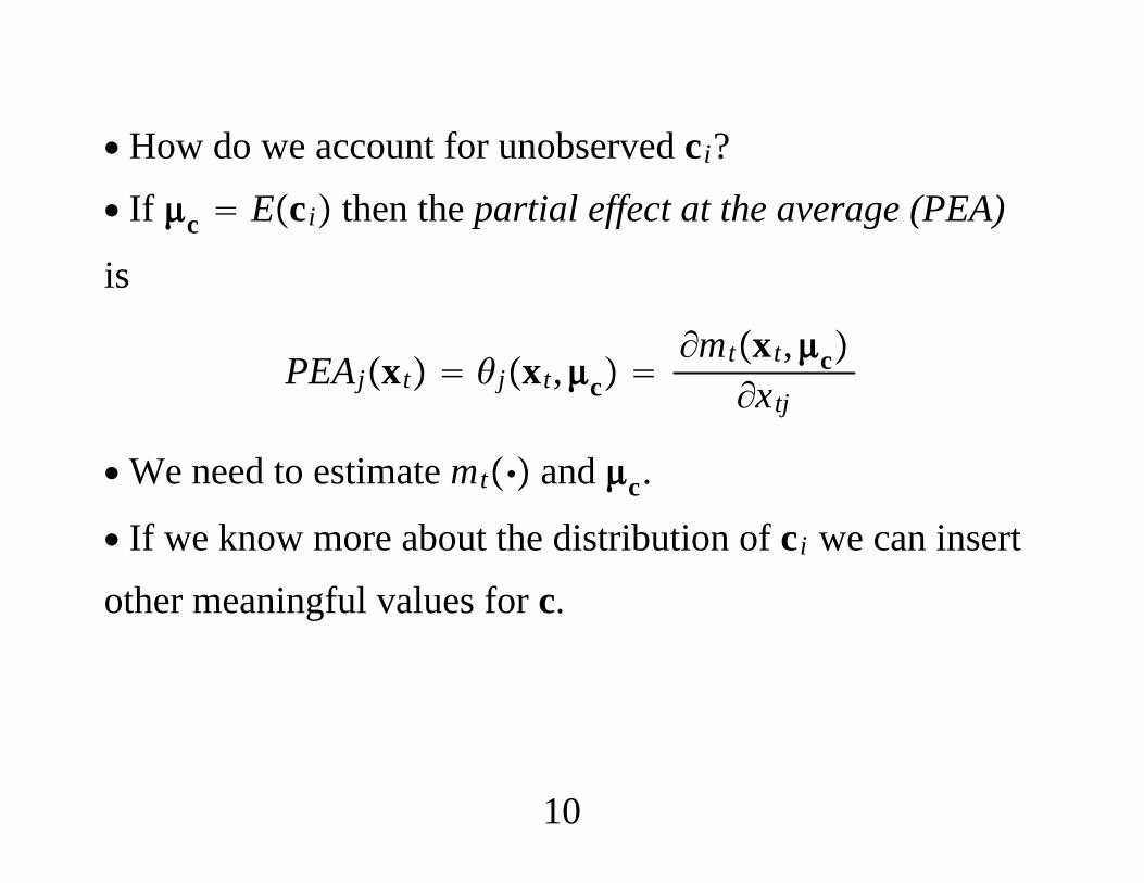
∙ How do we account for unobserved ci?∙ If c Eci then the partial effect at the average (PEA)
is
PEAjxt jxt,c ∂mtxt,c∂xtj
∙We need to estimate mt and c.
∙ If we know more about the distribution of ci we can insertother meaningful values for c.
10
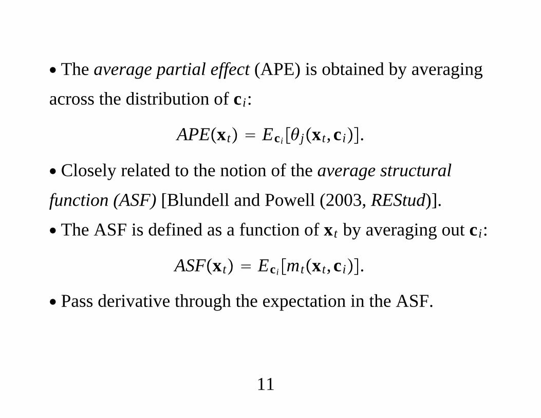
∙ The average partial effect (APE) is obtained by averagingacross the distribution of ci:
APExt Ecijxt,ci.
∙ Closely related to the notion of the average structuralfunction (ASF) [Blundell and Powell (2003, REStud)].∙ The ASF is defined as a function of xt by averaging out ci:
ASFxt Ecimtxt,ci.
∙ Pass derivative through the expectation in the ASF.
11
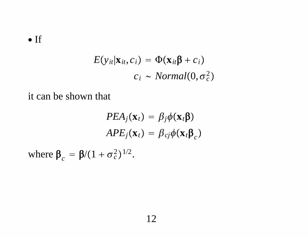
∙ If
Eyit|xit,ci xit ci
ci Normal0,c2
it can be shown that
PEAjxt jxt
APEjxt cjxtc
where c /1 c21/2.
12
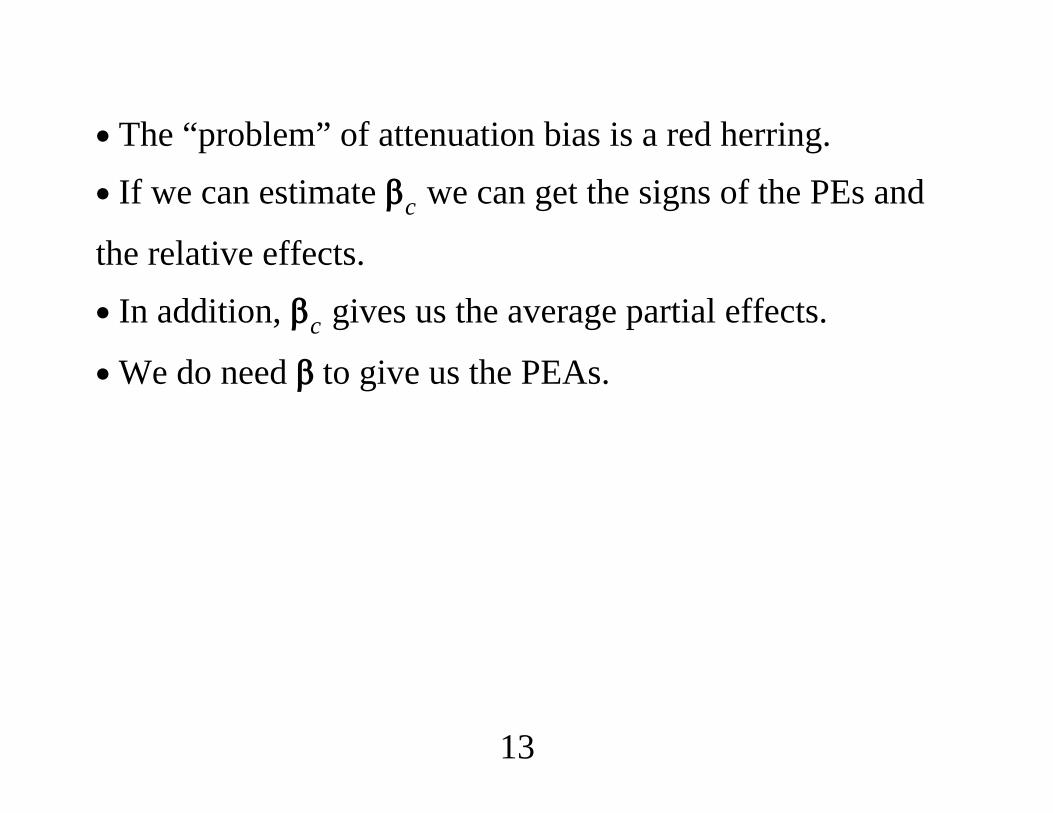
∙ The “problem” of attenuation bias is a red herring.∙ If we can estimate c we can get the signs of the PEs and
the relative effects.∙ In addition, c gives us the average partial effects.
∙We do need to give us the PEAs.
13

∙ Important: Definitions of partial effects do not depend onwhether xit is correlated with ci.∙ xit could include variables correlated with ci, includingyi,t−1.∙Whether we can estimate the PEs does depend on what weassume about the relationship beween ci and xit.∙ Focus on APEs means very general analyses are available– even nonparametric analyses. Altonji and Matzkin (2005,Econometrica).
14

3. Assumptions for Nonlinear ModelsAssumptions Relating xit : t 1, . . . ,T and Shocks∙ A general definition of strict exogeneity (conditional onthe heterogeneity) is
Dyit|xi1, . . . ,xiT,ci Dyit|xit,ci.
∙ In some cases strict exogeneity in the conditional mean issufficient.
15
Conditional Independence∙ In linear models, serial dependence of idiosyncratic shocksis easily dealt with by “cluster robust” inference.∙ Or, can use a GLS method. In the linear case with strictlyexogenous covariates, improperly modeled serial correlationnever results in inconsistent estimation.∙ Different with nonlinear models estimated by full MLE: Ifindependence is used it is usually needed for consistency.
16
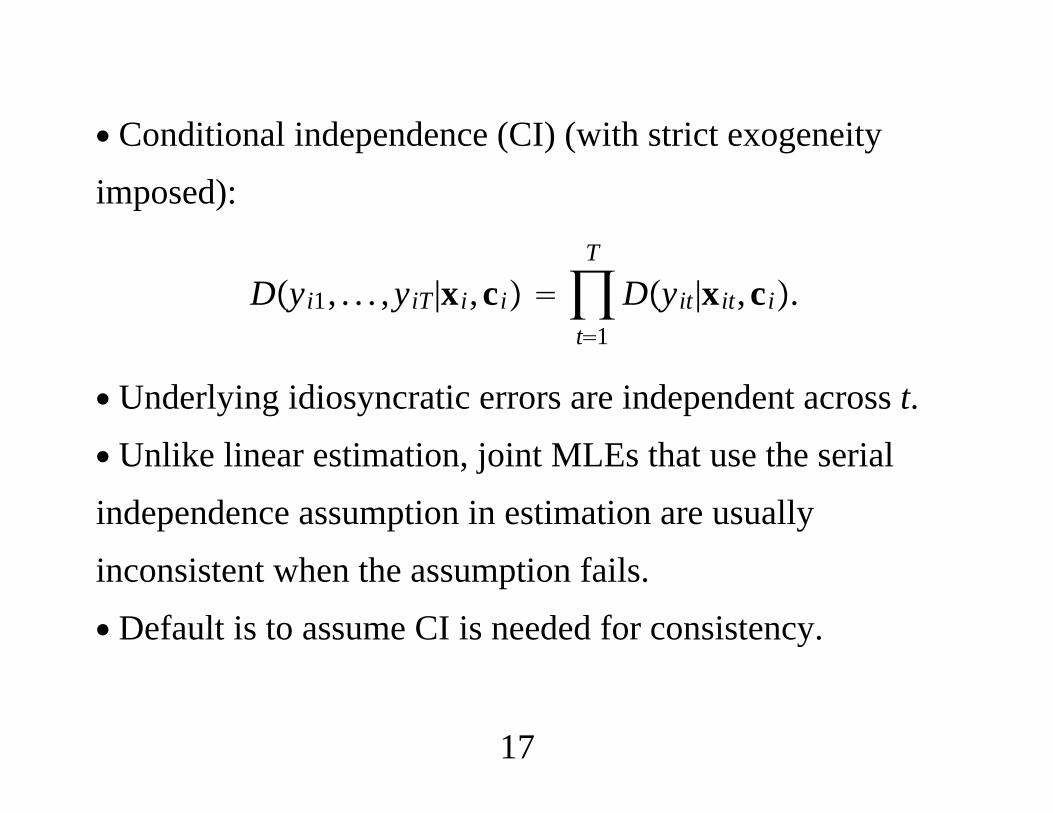
∙ Conditional independence (CI) (with strict exogeneityimposed):
Dyi1, . . . ,yiT|xi,ci t1
T
Dyit|xit,ci.
∙ Underlying idiosyncratic errors are independent across t.∙ Unlike linear estimation, joint MLEs that use the serialindependence assumption in estimation are usuallyinconsistent when the assumption fails.∙ Default is to assume CI is needed for consistency.
17

∙ In the CRE framework, CI plays a critical role in beingable to estimate the “structural” parameters and theparameters in the distribution of ci.∙ In a broad class of popular models, CI plays no essentialrole in estimating APEs using pooled methods.
18
Assumptions Relating ci and xit : t 1, . . . ,TRandom Effects∙ Generally stated, the key RE assumption is
Dci|xi1, . . . ,xiT Dci.
∙ Then Dci is modeled. The RE assumption is very strong.
19
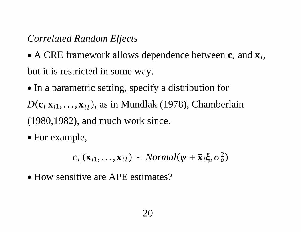
Correlated Random Effects∙ A CRE framework allows dependence between ci and xi,but it is restricted in some way.∙ In a parametric setting, specify a distribution forDci|xi1, . . . ,xiT, as in Mundlak (1978), Chamberlain(1980,1982), and much work since.∙ For example,
ci|xi1, . . . ,xiT Normal xi,a2
∙ How sensitive are APE estimates?
20
Fixed Effects∙ “Fixed effects” is used in two different ways.1. The ci, i 1, . . . ,N are parameters to be estimated alongwith fixed parameters. Usually leads to an “incidentalparameters problem” unless T is “large.”2. Dci|xi is unrestricted and we look for objectivefunctions that do not depend on ci but identify thepopulation parameters.
21

∙ Leads to “conditional MLE” (CMLE).∙ In the rare cases where CMLE is applicable, conditionalindependence is usually maintained.∙ PEAs and APEs are rarely identified by methods that useconditioning to eliminate ci. We can get directions andsometimes relative magnitudes, but not APEs.
22

Ideal FE CMLE CRE
Restricts Dci |xi? No No No Yes
Incidental Parameters with Small T? No Yes No No
Restricts Time Series Dependence/Heterogeneity? No Yes 1 Yes 2 No
Only Special Models? No No 3 Yes No
APEs Identified? Yes Yes 4 No Yes
Unbalanced Panels? Yes Yes Yes Yes 5
Can Estimate Dci? Yes Yes 4 No Yes 6
1. The large T approximations assume weak dependence and often stationarity.2. Usually conditional independence, unless estimator is inherently fully robust (linear, Poisson).3. Need at least one more time period than sources of heterogeneity.4. Subject to the incidental parameters problem.5. Subject to exchangeability restrictions.6. Under conditional independence or some other restriction.
23
4. Binary/Fractional Response ModelsCorrelated Random Effects Probit∙ The model is
Pyit 1|xit,ci xit ci, t 1, . . . ,T.
∙ Strict exogeneity conditional on ci:
Pyit 1|xi1, . . . ,xiT,ci Pyit 1|xit,ci
∙ Could have xit zit, . . . ,zi,t−Q.
24
∙ Conditional independence:
Dyi1, . . . ,yiT|xi,ci Dyi1|xi,ciDyiT|xi,ci
∙Model for Dci|xi:
ci xi ai, ai|xi Normal0,a2.
∙ Chamberlain: Replace xi with xi xi1, . . . ,xiT.
25

∙ Can obtain the first three assumptions from a latentvariable model:
yit 1xit ci uit 0uit|xit,ci Normal0,1
Duit|xi,ci Duit|xit,ci
uit : t 1, . . . ,T independent
26
∙With conditional independence we can estimate features ofthe unconditional distribution of ci:
c x
c2 ≡
′ N−1∑i1
N
xi − x′xi − x a2
∙ Can evaluate PEs at c, or insert c kc for various k.
27
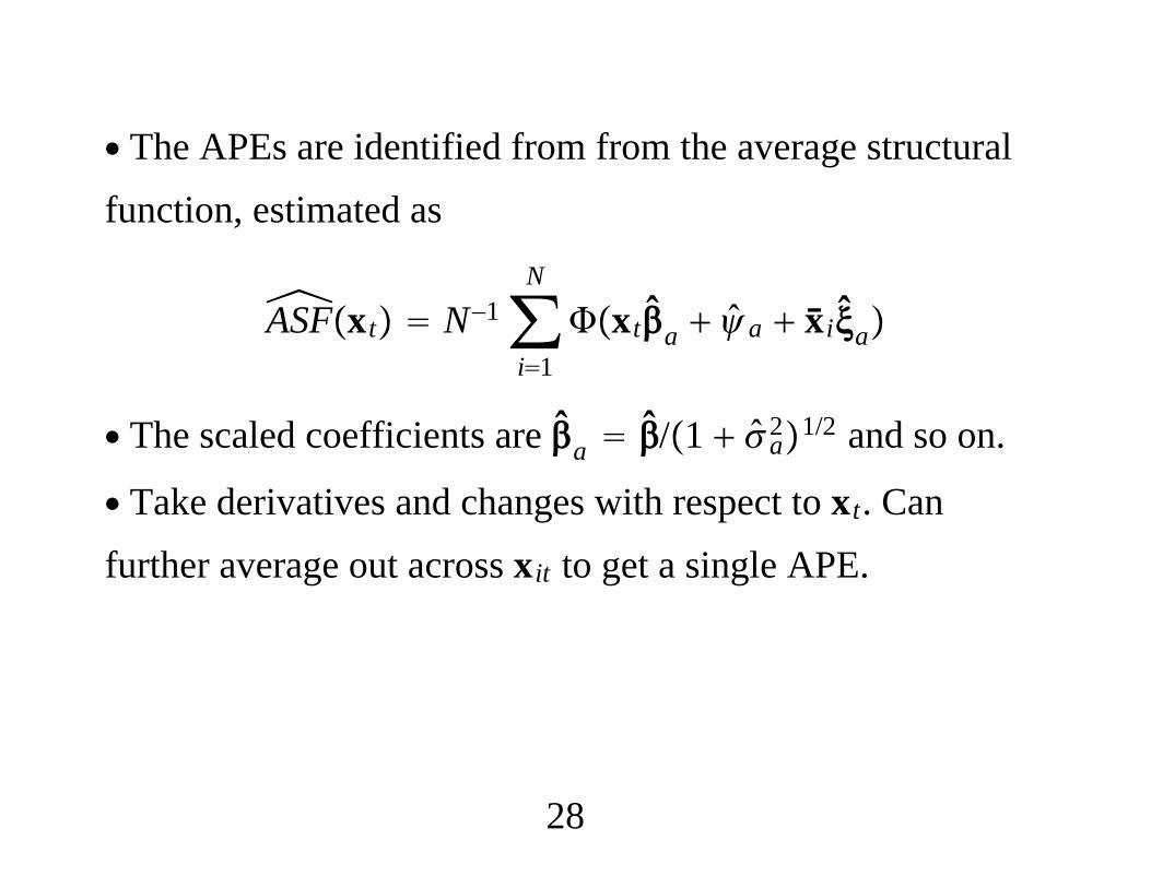
∙ The APEs are identified from from the average structuralfunction, estimated as
ASFxt N−1∑i1
N
xta a xia
∙ The scaled coefficients are a /1 a21/2 and so on.
∙ Take derivatives and changes with respect to xt. Canfurther average out across xit to get a single APE.
28

∙ Conditional independence is strong, and the joint MLE isnot robust to its violation. (Contrast RE estimation of thelinear model.)∙ If we focus on APEs, can use pooled probit method anddrop the serial independence assumption.∙ Pooled probit estimates the scaled coefficients directlybecause
Pyit 1|xi Pyit 1|xit, xi
xita a xia.
29
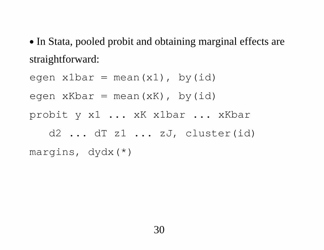
∙ In Stata, pooled probit and obtaining marginal effects arestraightforward:egen x1bar mean(x1), by(id)
egen xKbar mean(xK), by(id)
probit y x1 ... xK x1bar ... xKbar
d2 ... dT z1 ... zJ, cluster(id)
margins, dydx(*)
30
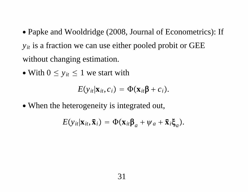
∙ Papke and Wooldridge (2008, Journal of Econometrics): Ifyit is a fraction we can use either pooled probit or GEEwithout changing estimation.∙With 0 ≤ yit ≤ 1 we start with
Eyit|xit,ci xit ci.
∙When the heterogeneity is integrated out,
Eyit|xit, xi xita a xia.
31
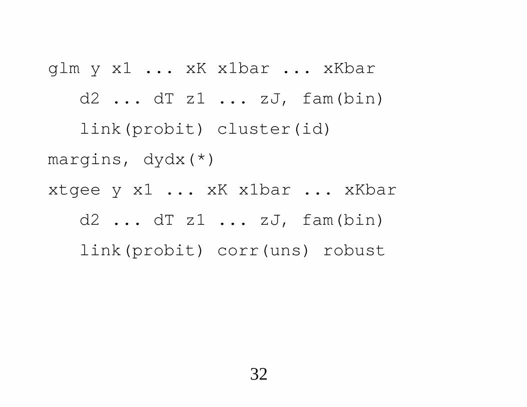
glm y x1 ... xK x1bar ... xKbar
d2 ... dT z1 ... zJ, fam(bin)
link(probit) cluster(id)
margins, dydx(*)
xtgee y x1 ... xK x1bar ... xKbar
d2 ... dT z1 ... zJ, fam(bin)
link(probit) corr(uns) robust
32
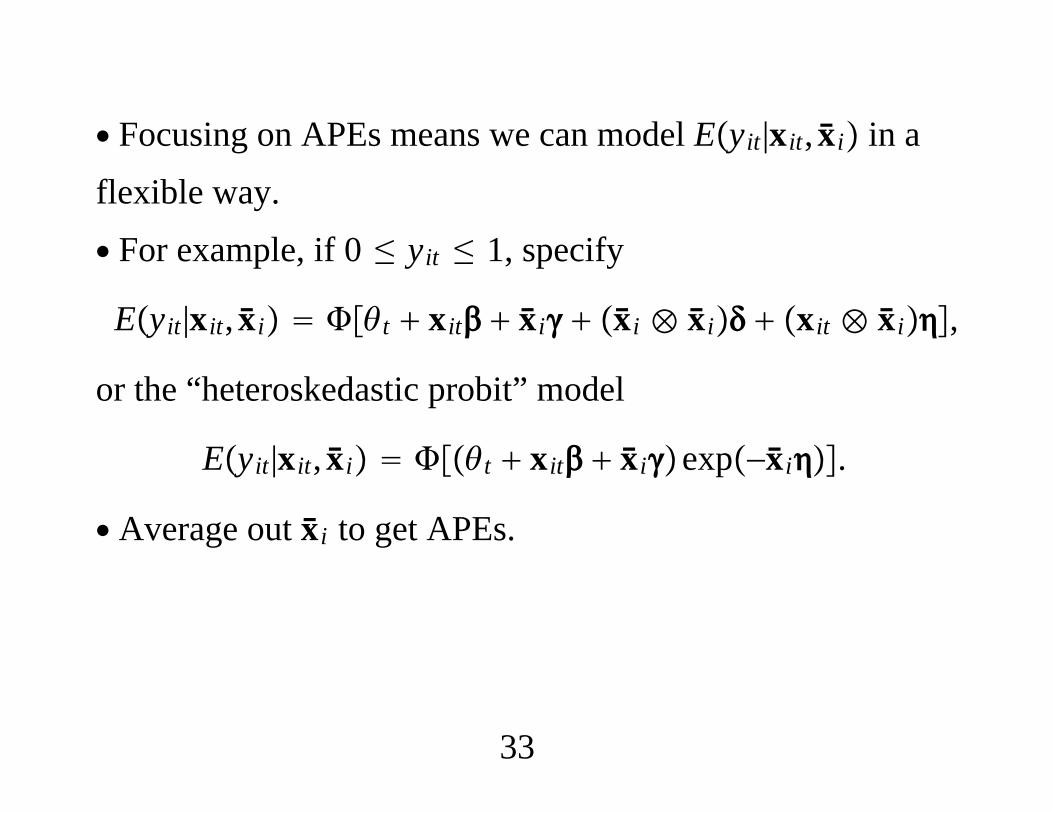
∙ Focusing on APEs means we can model Eyit|xit, xi in aflexible way.∙ For example, if 0 ≤ yit ≤ 1, specify
Eyit|xit, xi t xit xi xi ⊗ xi xit ⊗ xi,
or the “heteroskedastic probit” model
Eyit|xit, xi t xit xiexp−xi.
∙ Average out xi to get APEs.
33
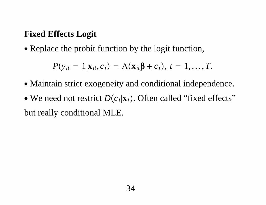
Fixed Effects Logit∙ Replace the probit function by the logit function,
Pyit 1|xit,ci xit ci, t 1, . . . ,T.
∙Maintain strict exogeneity and conditional independence.∙We need not restrict Dci|xi. Often called “fixed effects”but really conditional MLE.
34
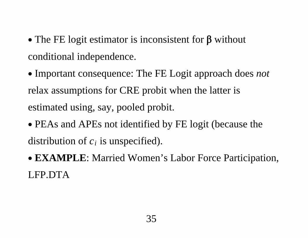
∙ The FE logit estimator is inconsistent for without
conditional independence.∙ Important consequence: The FE Logit approach does notrelax assumptions for CRE probit when the latter isestimated using, say, pooled probit.∙ PEAs and APEs not identified by FE logit (because thedistribution of ci is unspecified).∙ EXAMPLE: Married Women’s Labor Force Participation,LFP.DTA
35
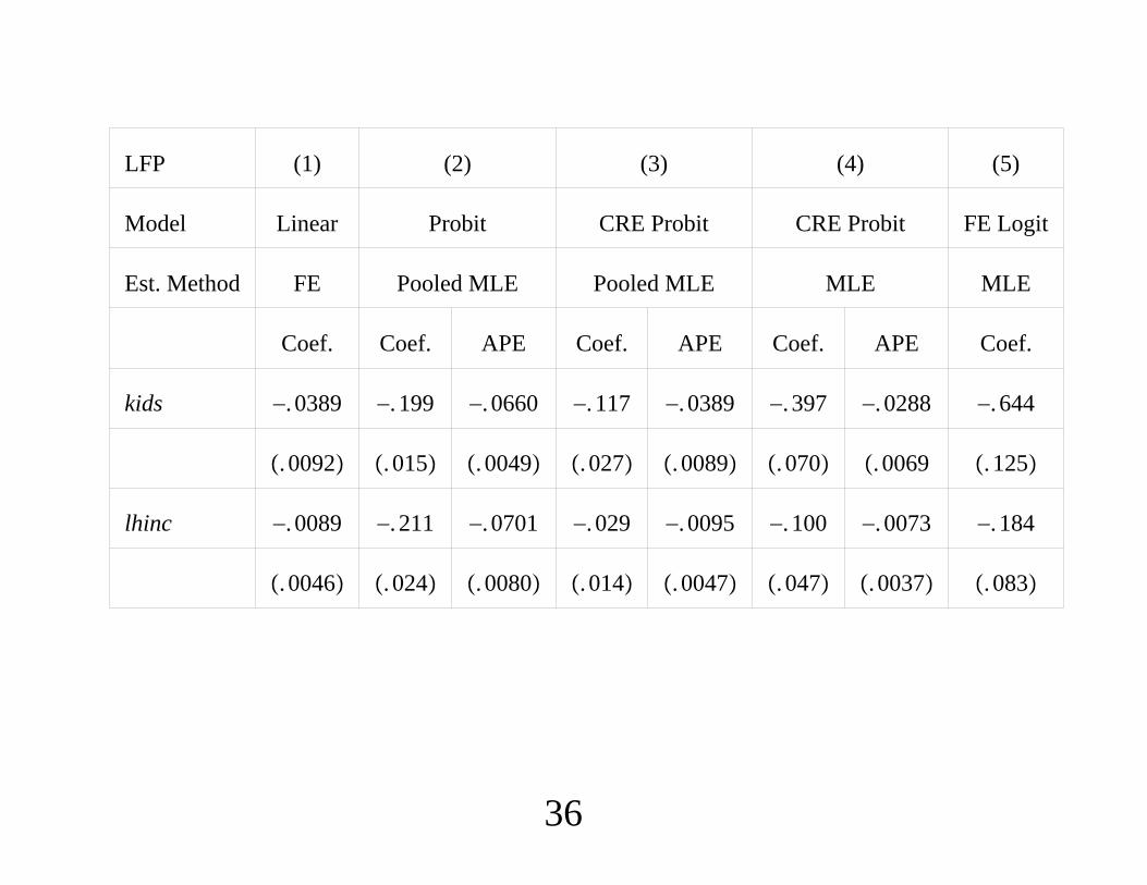
LFP (1) (2) (3) (4) (5)
Model Linear Probit CRE Probit CRE Probit FE Logit
Est. Method FE Pooled MLE Pooled MLE MLE MLE
Coef. Coef. APE Coef. APE Coef. APE Coef.
kids −. 0389 −. 199 −. 0660 −. 117 −. 0389 −. 397 −. 0288 −. 644
. 0092 . 015 . 0049 . 027 . 0089 . 070 . 0069 . 125
lhinc −. 0089 −. 211 −. 0701 −. 029 −. 0095 −. 100 −. 0073 −. 184
. 0046 . 024 . 0080 . 014 . 0047 . 047 . 0037 . 083
36
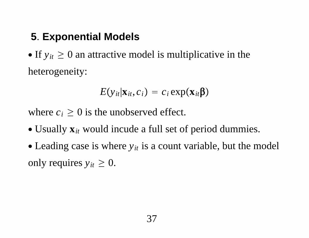
5. Exponential Models∙ If yit ≥ 0 an attractive model is multiplicative in theheterogeneity:
Eyit|xit,ci ci expxit
where ci ≥ 0 is the unobserved effect.∙ Usually xit would incude a full set of period dummies.∙ Leading case is where yit is a count variable, but the modelonly requires yit ≥ 0.
37
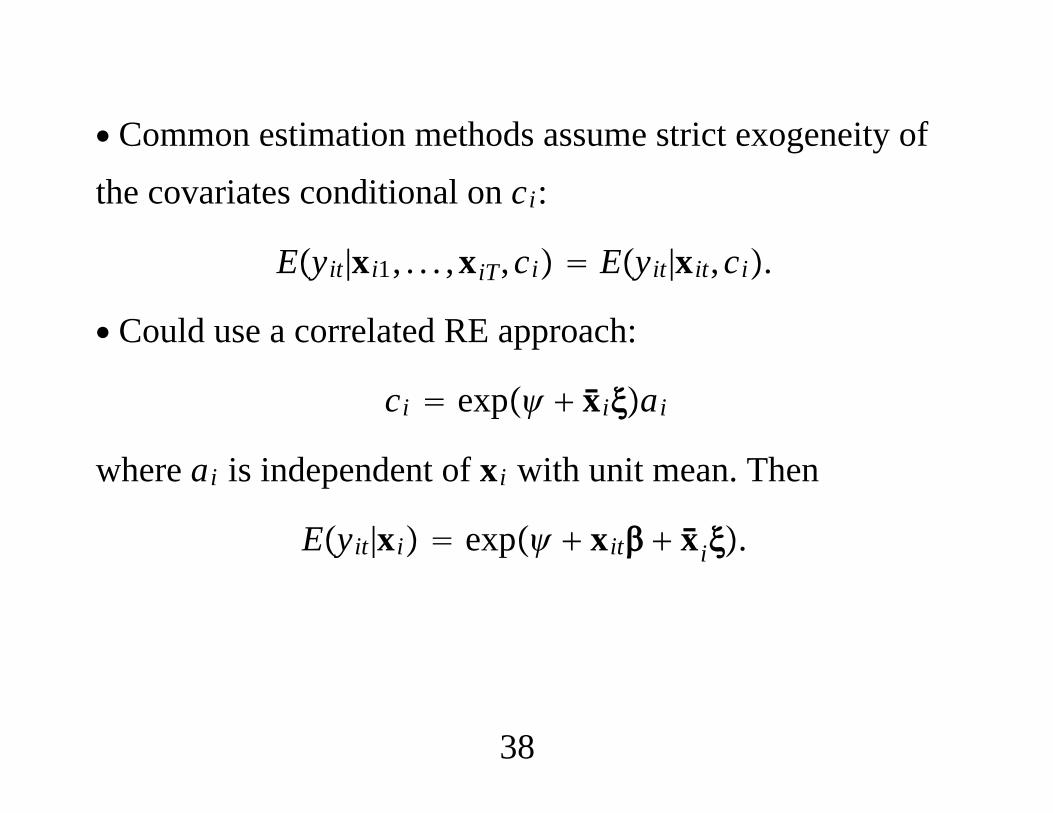
∙ Common estimation methods assume strict exogeneity ofthe covariates conditional on ci:
Eyit|xi1, . . . ,xiT,ci Eyit|xit,ci.
∙ Could use a correlated RE approach:
ci exp xiai
where ai is independent of xi with unit mean. Then
Eyit|xi exp xit xi.
38

∙ The most robust estimator is the “fixed effects Poisson”estimator, which was originally derived as a conditionalMLE under strong assumptions.∙ Important Result: The FE Poisson estimator is consistentunder
Eyit|xi,ci Eyit|xit,ci ci expxit.
only.∙ The Poisson distribution can be arbitrarily misspecified,and any kind of serial correlation can be present.
39
∙ yit need not even be a count variable. It could becontinuous, or a corner solution. The mean functionci expxit should make logical sense.
∙Whether or not yit is a count, should make inference fullyrobust to serial correlation and violation of the Poissondistribution.∙ Stata:xtpoisson y x1 ... xK, fe vce(robust)
40
∙Why not FE Negative Binomial?1. FE NegBin imposes a very specific version ofoverdispersion for each unit i:
Varyit|xi,ci 1 ciEyit|xi,ci
2. FE NegBin imposes conditional independence.3. It is not known to be robust to failure of eitherassumption.
41
∙ For getting effects on the mean, FE Poisson is preferredbecause it is fully robust and robust inference is now easilyavailable.∙ Can use GMM to impose higher order momentassumptions for improved efficiency.∙ Even if the FE NegBin estimates are close to FE Poisson,inference for NegBin might be very misleading.
42
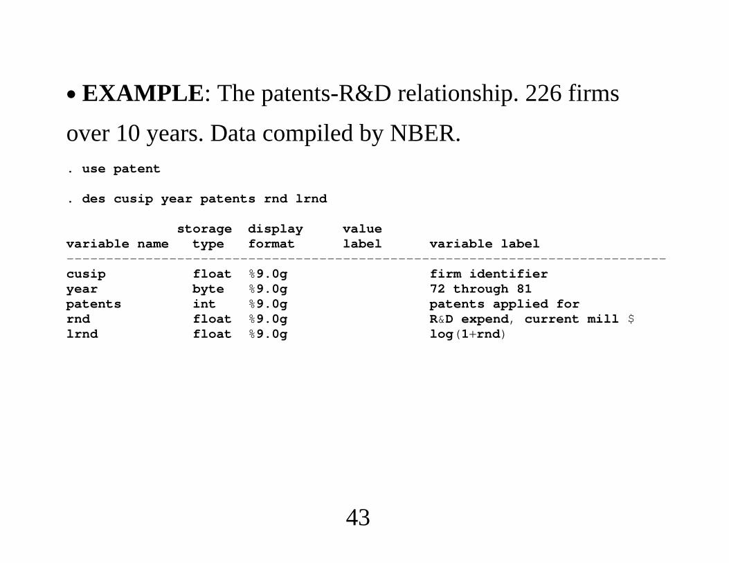
∙ EXAMPLE: The patents-R&D relationship. 226 firmsover 10 years. Data compiled by NBER.. use patent
. des cusip year patents rnd lrnd
storage display valuevariable name type format label variable label----------------------------------------------------------------------------cusip float %9.0g firm identifieryear byte %9.0g 72 through 81patents int %9.0g patents applied forrnd float %9.0g R&D expend, current mill $lrnd float %9.0g log(1rnd)
43
. xtreg patents lrnd lrnd_1 lrnd_2 lrnd_3 lrnd_4 lrnd_5 lrnd_6 y79-y81,fe cluster(cusip)
Fixed-effects (within) regression Number of obs 904Group variable: cusip Number of groups 226
(Std. Err. adjusted for 226 clusters in cusip----------------------------------------------------------------------------
| Robustpatents | Coef. Std. Err. t P|t| [95% Conf. Interval
---------------------------------------------------------------------------lrnd | -4.891047 4.487274 -1.09 0.277 -13.73351 3.951412
lrnd_1 | -8.770371 5.825649 -1.51 0.134 -20.25018 2.70944lrnd_2 | -1.399383 3.024928 -0.46 0.644 -7.360195 4.561428lrnd_3 | -3.218844 3.173328 -1.01 0.312 -9.472087 3.034399lrnd_4 | -8.89406 4.729909 -1.88 0.061 -18.21464 .4265244lrnd_5 | -4.574966 5.090455 -0.90 0.370 -14.60603 5.456098lrnd_6 | -13.7178 6.755444 -2.03 0.043 -27.02983 -.4057713
y79 | 2.282507 1.051129 2.17 0.031 .2111897 4.353824y80 | .6192547 1.261851 0.49 0.624 -1.867302 3.105811y81 | -9.543918 2.827286 -3.38 0.001 -15.11526 -3.972572
_cons | 93.2246 18.58406 5.02 0.000 56.60353 129.8457---------------------------------------------------------------------------
44
. * Pooled Poisson but no heterogeneity:
. poisson patents lrnd lrnd_1 lrnd_2 lrnd_3 lrnd_4 lrnd_5 lrnd_6 y79-y81,cluster(cusip)
Poisson regression Number of obs 904
(Std. Err. adjusted for 226 clusters in cusip----------------------------------------------------------------------------
| Robustpatents | Coef. Std. Err. z P|z| [95% Conf. Interval
---------------------------------------------------------------------------lrnd | .7310869 .3421723 2.14 0.033 .0604416 1.401732
lrnd_1 | -.3529964 .3324251 -1.06 0.288 -1.004538 .2985449lrnd_2 | -.2556217 .4482509 -0.57 0.568 -1.134177 .6229339lrnd_3 | .5953963 .5041567 1.18 0.238 -.3927328 1.583525lrnd_4 | .3925039 .2426363 1.62 0.106 -.0830545 .8680624lrnd_5 | -.0209466 .3541238 -0.06 0.953 -.7150165 .6731232lrnd_6 | -.3143883 .436545 -0.72 0.471 -1.170001 .5412242
y79 | -.1004726 .0618751 -1.62 0.104 -.2217455 .0208004y80 | -.4389727 .0639321 -6.87 0.000 -.5642773 -.3136681y81 | -1.871174 .0994861 -18.81 0.000 -2.066163 -1.676185
_cons | .8720311 .2072225 4.21 0.000 .4658825 1.27818----------------------------------------------------------------------------
45
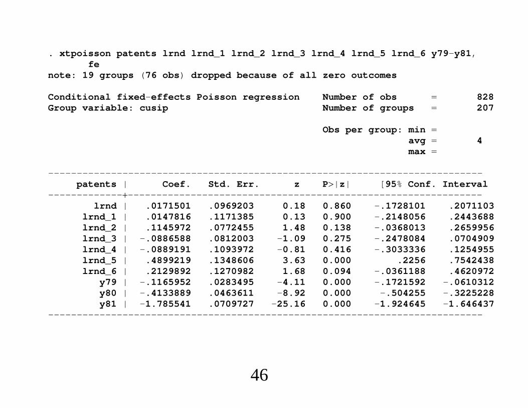
. xtpoisson patents lrnd lrnd_1 lrnd_2 lrnd_3 lrnd_4 lrnd_5 lrnd_6 y79-y81,fe
note: 19 groups (76 obs) dropped because of all zero outcomes
Conditional fixed-effects Poisson regression Number of obs 828Group variable: cusip Number of groups 207
Obs per group: min avg 4max
----------------------------------------------------------------------------patents | Coef. Std. Err. z P|z| [95% Conf. Interval
---------------------------------------------------------------------------lrnd | .0171501 .0969203 0.18 0.860 -.1728101 .2071103
lrnd_1 | .0147816 .1171385 0.13 0.900 -.2148056 .2443688lrnd_2 | .1145972 .0772455 1.48 0.138 -.0368013 .2659956lrnd_3 | -.0886588 .0812003 -1.09 0.275 -.2478084 .0704909lrnd_4 | -.0889191 .1093972 -0.81 0.416 -.3033336 .1254955lrnd_5 | .4899219 .1348606 3.63 0.000 .2256 .7542438lrnd_6 | .2129892 .1270982 1.68 0.094 -.0361188 .4620972
y79 | -.1165952 .0283495 -4.11 0.000 -.1721592 -.0610312y80 | -.4133889 .0463611 -8.92 0.000 -.504255 -.3225228y81 | -1.785541 .0709727 -25.16 0.000 -1.924645 -1.646437
----------------------------------------------------------------------------
46
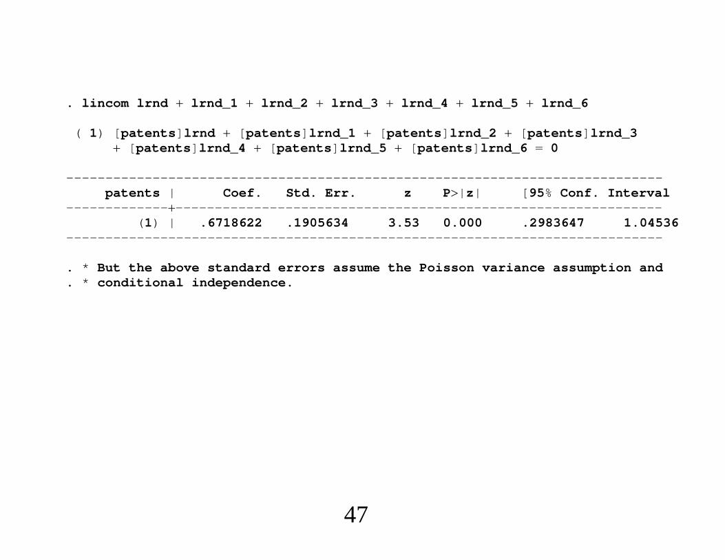
. lincom lrnd lrnd_1 lrnd_2 lrnd_3 lrnd_4 lrnd_5 lrnd_6
( 1) [patents]lrnd [patents]lrnd_1 [patents]lrnd_2 [patents]lrnd_3 [patents]lrnd_4 [patents]lrnd_5 [patents]lrnd_6 0
----------------------------------------------------------------------------patents | Coef. Std. Err. z P|z| [95% Conf. Interval
---------------------------------------------------------------------------(1) | .6718622 .1905634 3.53 0.000 .2983647 1.04536
----------------------------------------------------------------------------
. * But the above standard errors assume the Poisson variance assumption and
. * conditional independence.
47
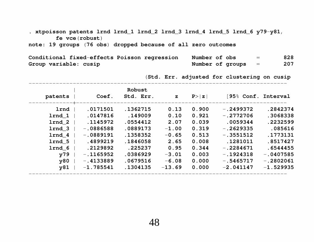
. xtpoisson patents lrnd lrnd_1 lrnd_2 lrnd_3 lrnd_4 lrnd_5 lrnd_6 y79-y81,fe vce(robust)
note: 19 groups (76 obs) dropped because of all zero outcomes
Conditional fixed-effects Poisson regression Number of obs 828Group variable: cusip Number of groups 207
(Std. Err. adjusted for clustering on cusip----------------------------------------------------------------------------
| Robustpatents | Coef. Std. Err. z P|z| [95% Conf. Interval
---------------------------------------------------------------------------lrnd | .0171501 .1362715 0.13 0.900 -.2499372 .2842374
lrnd_1 | .0147816 .149009 0.10 0.921 -.2772706 .3068338lrnd_2 | .1145972 .0554412 2.07 0.039 .0059344 .2232599lrnd_3 | -.0886588 .0889173 -1.00 0.319 -.2629335 .085616lrnd_4 | -.0889191 .1358352 -0.65 0.513 -.3551512 .1773131lrnd_5 | .4899219 .1846058 2.65 0.008 .1281011 .8517427lrnd_6 | .2129892 .225237 0.95 0.344 -.2284671 .6544455
y79 | -.1165952 .0386929 -3.01 0.003 -.1924318 -.0407585y80 | -.4133889 .0679516 -6.08 0.000 -.5465717 -.2802061y81 | -1.785541 .1304135 -13.69 0.000 -2.041147 -1.529935
----------------------------------------------------------------------------
48
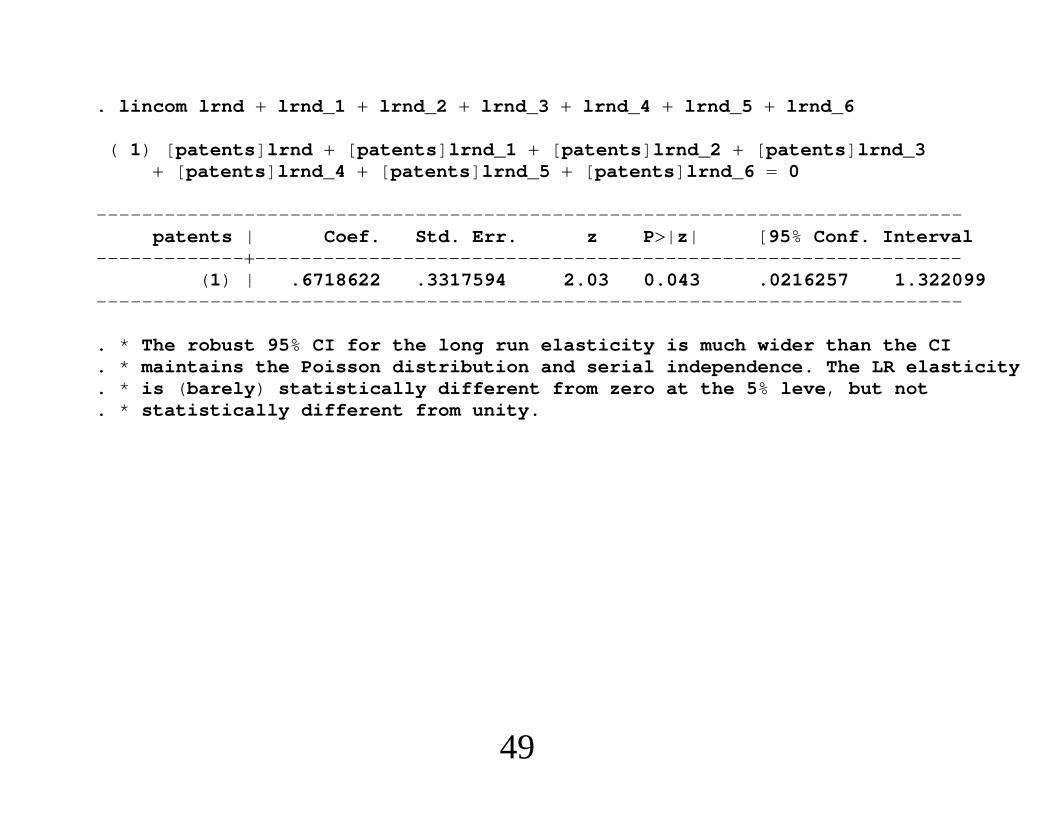
. lincom lrnd lrnd_1 lrnd_2 lrnd_3 lrnd_4 lrnd_5 lrnd_6
( 1) [patents]lrnd [patents]lrnd_1 [patents]lrnd_2 [patents]lrnd_3 [patents]lrnd_4 [patents]lrnd_5 [patents]lrnd_6 0
----------------------------------------------------------------------------patents | Coef. Std. Err. z P|z| [95% Conf. Interval
---------------------------------------------------------------------------(1) | .6718622 .3317594 2.03 0.043 .0216257 1.322099
----------------------------------------------------------------------------
. * The robust 95% CI for the long run elasticity is much wider than the CI
. * maintains the Poisson distribution and serial independence. The LR elasticity
. * is (barely) statistically different from zero at the 5% leve, but not
. * statistically different from unity.
49
6. Dynamic Models∙ Difficult to specify and estimate models with heterogeneityif we only assume sequential exogeneity.∙ Generally, have to model feedback mechanisms.∙ Completely specified dynamic models with can beestimated under certain assumptions.
50
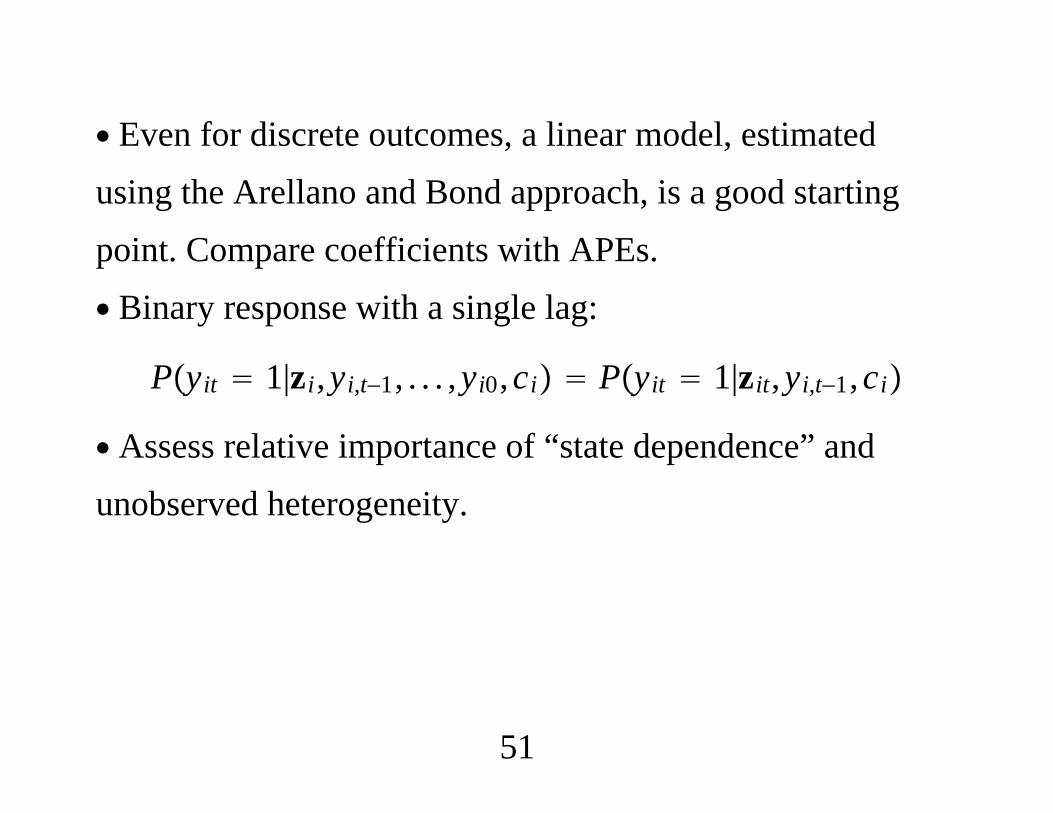
∙ Even for discrete outcomes, a linear model, estimatedusing the Arellano and Bond approach, is a good startingpoint. Compare coefficients with APEs.∙ Binary response with a single lag:
Pyit 1|zi,yi,t−1, . . . ,yi0,ci Pyit 1|zit,yi,t−1,ci
∙ Assess relative importance of “state dependence” andunobserved heterogeneity.
51
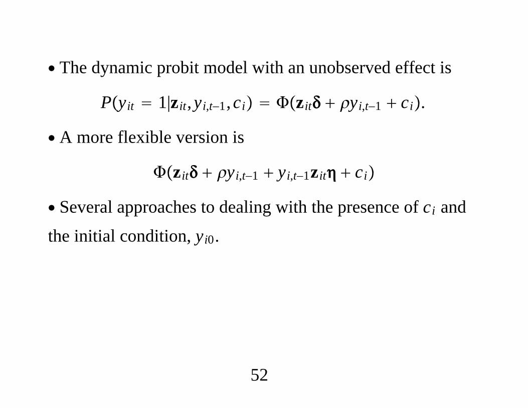
∙ The dynamic probit model with an unobserved effect is
Pyit 1|zit,yi,t−1,ci zit yi,t−1 ci.
∙ A more flexible version is
zit yi,t−1 yi,t−1zit ci
∙ Several approaches to dealing with the presence of ci andthe initial condition, yi0.
52
(i) Treat the ci as parameters to estimate: Incidentalparameters problem and computationally intensive.(ii) Try to estimate and without specifying conditional or
unconditional distributions for ci: Available only in specialcases. Cannot estimate partial effects.
53
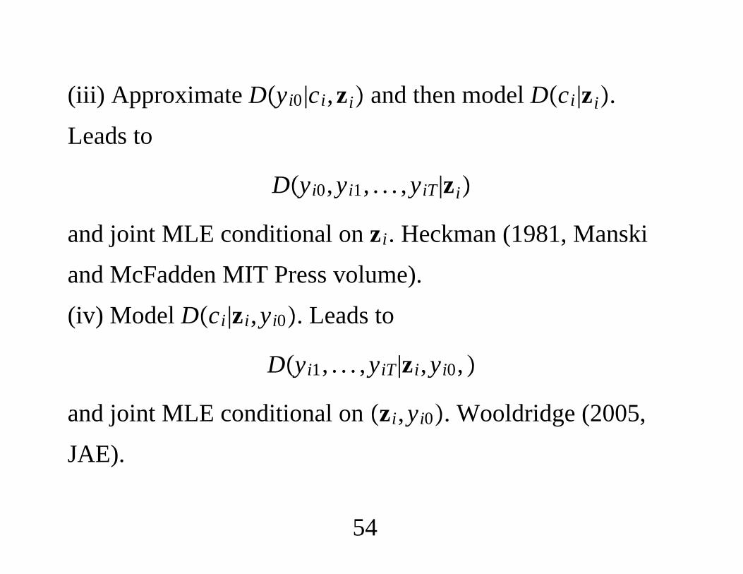
(iii) Approximate Dyi0|ci,zi and then model Dci|zi.
Leads to
Dyi0,yi1, . . . ,yiT|zi
and joint MLE conditional on zi. Heckman (1981, Manskiand McFadden MIT Press volume).(iv) Model Dci|zi,yi0. Leads to
Dyi1, . . . ,yiT|zi,yi0,
and joint MLE conditional on zi,yi0. Wooldridge (2005,JAE).
54
∙ Average partial effects are generally identified, and inleading cases take simple forms.∙With large N and small T, the panel data bootstrap(resampling all time periods from the cross-sectional units)can be used for standard errors and inference.
55
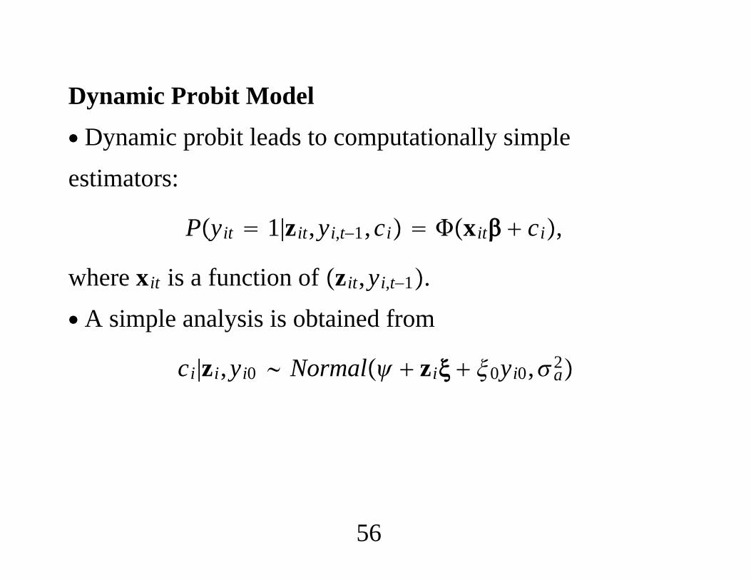
Dynamic Probit Model∙ Dynamic probit leads to computationally simpleestimators:
Pyit 1|zit,yi,t−1,ci xit ci,
where xit is a function of zit,yi,t−1.∙ A simple analysis is obtained from
ci|zi,yi0 Normal zi 0yi0,a2
56
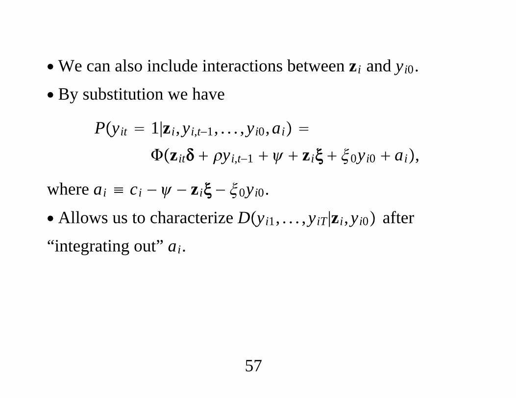
∙We can also include interactions between zi and yi0.∙ By substitution we have
Pyit 1|zi,yi,t−1, . . . ,yi0,ai
zit yi,t−1 zi 0yi0 ai,
where ai ≡ ci − − zi − 0yi0.
∙ Allows us to characterize Dyi1, . . . ,yiT|zi,yi0 after“integrating out” ai.
57
∙ The likelihood function has the same form as when thexit are strictly exogenous.∙We can use standard random effects probit software, wherethe explanatory variables in time t are 1,zit,yi,t−1,zi,yi0, .∙ Tempting, but wrong, to apply pooled probit withexplanatory variables 1,zit,yi,t−1,zi,yi0, .
58
∙ Easily get the average partial effects, too:
ASFzt,yt−1 N−1∑i1
N
zta ayt−1 a
zia a0yi0
and take differences or derivatives with respect to elementsof zt,yt−1.
∙ The scaled coefficients are a 1 a2−1/2.
59

EXAMPLE: (Dynamic Married Women’s Labor ForceParticipation)
Plfpit 1|kidsit, lhincit, lfpi,t−1,ci
t 1kidsit 2lhincit lfpi,t−1 ci
ci|zi, lfpi0 Normal zi 0lfpi0,a2
∙ To measure the magnitude of state dependence, estimate
Ecit 1kidst 2lhinct ci
− t 1kidst 2lhinct ci
and put in interesting values for kidst and lhinct.
60
∙ Data from LFP.DTA.∙ The APE from dynamic probit with heterogeneity is about. 260 se . 026. If we ignore the heterogeneity, estimatedAPE is . 837 se . 005; standard errors from 500 panelbootstrap replications.∙ Linear model estimates: . 382 se . 020 withheterogeneity, . 851 se . 004 without.
61
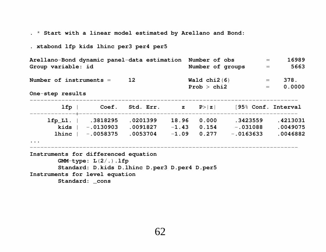
. * Start with a linear model estimated by Arellano and Bond:
. xtabond lfp kids lhinc per3 per4 per5
Arellano-Bond dynamic panel-data estimation Number of obs 16989Group variable: id Number of groups 5663
Number of instruments 12 Wald chi2(6) 378.Prob chi2 0.0000
One-step results----------------------------------------------------------------------------
lfp | Coef. Std. Err. z P|z| [95% Conf. Interval---------------------------------------------------------------------------
lfp_L1. | .3818295 .0201399 18.96 0.000 .3423559 .4213031kids | -.0130903 .0091827 -1.43 0.154 -.031088 .0049075
lhinc | -.0058375 .0053704 -1.09 0.277 -.0163633 .0046882...----------------------------------------------------------------------------Instruments for differenced equation
GMM-type: L(2/.).lfpStandard: D.kids D.lhinc D.per3 D.per4 D.per5
Instruments for level equationStandard: _cons
62
. * Accounting for heterogeneity is important, even in the linear
. * approximation:
. reg lfp l.lfp kids lhinc per3 per4 per5, robust
Linear regression Number of obs 22652F( 6, 22645) 7938.Prob F 0.0000R-squared 0.7207Root MSE .24664
----------------------------------------------------------------------------| Robust
lfp | Coef. Std. Err. t P|t| [95% Conf. Interval---------------------------------------------------------------------------
lfp |L1. | .8510015 .0039478 215.57 0.000 .8432637 .8587394
|kids | -.0021431 .0014379 -1.49 0.136 -.0049615 .0006754
lhinc | -.0071892 .0025648 -2.80 0.005 -.0122164 -.0021619...---------------------------------------------------------------------------
63
. * Generate variables needed for dynamic probit.
tsset id period
* Lagged dependent variable:bysort id (period): gen lfp_1 L.lfp* Put initial condition in periods 2-5:by id: gen lfp1 lfp[1]* Create kids variables for periods 2-5:forv i2/5 by id: gen kids‘i’ kids[‘i’]* Create lhinc variables for periods 2-5:forv i2/5 by id: gen lhinc‘i’ lhinc[‘i’]
* Could include kids1 and lhinc1 as well, in which case change loop* to i1/5.
64
. * Now full RE probit:
.
. xtprobit lfp lfp_1 lfp1 kids kids2-kids5 lhinc lhinc2-lhinc5 educblack age agesq per3-per5, re
Random-effects probit regression Number of obs 22652Group variable (i): id Number of groups 5663
Wald chi2(19) 4091.Log likelihood -5028.9785 Prob chi2 0.0000
----------------------------------------------------------------------------lfp | Coef. Std. Err. z P|z| [95% Conf. Interval
---------------------------------------------------------------------------lfp_1 | 1.541288 .066803 23.07 0.000 1.410357 1.67222
lfp1 | 2.530053 .1565322 16.16 0.000 2.223256 2.836851kids | -.1455379 .0787386 -1.85 0.065 -.2998626 .0087868
kids2 | .3236282 .0968499 3.34 0.001 .133806 .5134504kids3 | .1072842 .1235197 0.87 0.385 -.1348099 .3493784kids4 | .01792 .1275595 0.14 0.888 -.2320921 .2679322kids5 | -.3912412 .1058482 -3.70 0.000 -.5986998 -.1837825
65
lhinc | -.0748846 .0508406 -1.47 0.141 -.1745304 .0247612lhinc2 | -.0232267 .0590167 -0.39 0.694 -.1388973 .0924438lhinc3 | -.083386 .0626056 -1.33 0.183 -.2060908 .0393188lhinc4 | -.0862979 .060961 -1.42 0.157 -.2057793 .0331835lhinc5 | .0627793 .0592742 1.06 0.290 -.053396 .1789547
educ | .049906 .0100314 4.97 0.000 .0302447 .0695672black | .1316009 .0982941 1.34 0.181 -.061052 .3242539
age | .1278946 .0193999 6.59 0.000 .0898715 .1659177agesq | -.0016882 .00024 -7.03 0.000 -.0021586 -.0012177
per3 | -.0560723 .0458349 -1.22 0.221 -.1459071 .0337625per4 | -.029532 .0463746 -0.64 0.524 -.1204245 .0613605per5 | -.0784793 .0464923 -1.69 0.091 -.1696025 .012644
_cons | -2.946082 .4367068 -6.75 0.000 -3.802011 -2.090152---------------------------------------------------------------------------
/lnsig2u | .0982792 .1225532 -.1419206 .338479---------------------------------------------------------------------------
sigma_u | 1.050367 .0643629 .9314989 1.184404rho | .52455 .0305644 .4645793 .583821
----------------------------------------------------------------------------Likelihood-ratio test of rho0: chibar2(01) 160.73 Prob chibar2 0.000
66

. predict xdh, xb
. gen xd0 xdh - _b[lfp_1]*lfp_1
. gen xd1 xd0 _b[lfp_1]
. gen xd0a xd0/sqrt(1 e(sigma_u)^2)
. gen xd1a xd1/sqrt(1 e(sigma_u)^2)
. gen PHI0 norm(xd0a)
. gen PHI1 norm(xd1a)
. gen pelfp_1 PHI1 - PHI0
. sum pelfp_1
Variable | Obs Mean Std. Dev. Min Max---------------------------------------------------------------------
pelfp_1 | 22652 .2591284 .0551711 .0675151 .4047995
. * .259 is the average probability of being in the labor force in
. * period t, given participation in t-1. This is somewhat lower than
. * the linear model estimate, .382.
67
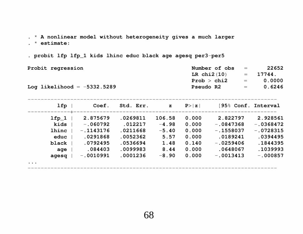
. * A nonlinear model without heterogeneity gives a much larger
. * estimate:
. probit lfp lfp_1 kids lhinc educ black age agesq per3-per5
Probit regression Number of obs 22652LR chi2(10) 17744.Prob chi2 0.0000
Log likelihood -5332.5289 Pseudo R2 0.6246
----------------------------------------------------------------------------lfp | Coef. Std. Err. z P|z| [95% Conf. Interval
---------------------------------------------------------------------------lfp_1 | 2.875679 .0269811 106.58 0.000 2.822797 2.928561
kids | -.060792 .012217 -4.98 0.000 -.0847368 -.0368472lhinc | -.1143176 .0211668 -5.40 0.000 -.1558037 -.0728315
educ | .0291868 .0052362 5.57 0.000 .0189241 .0394495black | .0792495 .0536694 1.48 0.140 -.0259406 .1844395
age | .084403 .0099983 8.44 0.000 .0648067 .1039993agesq | -.0010991 .0001236 -8.90 0.000 -.0013413 -.000857
...----------------------------------------------------------------------------
68
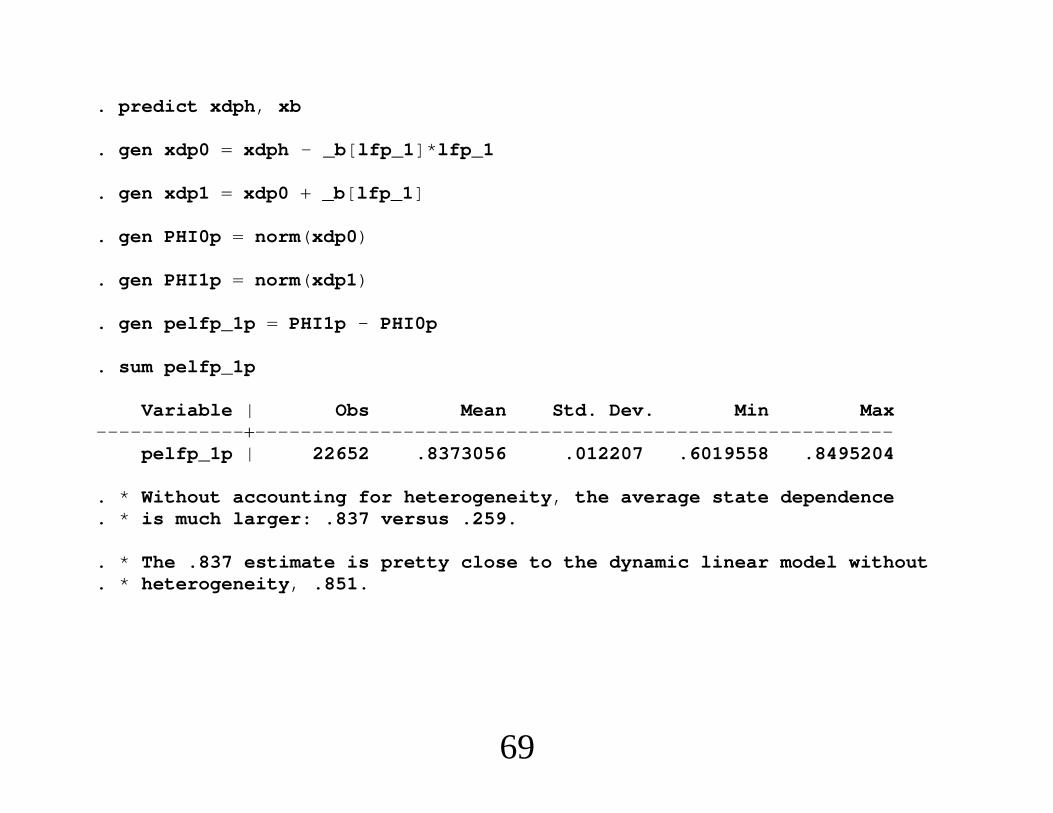
. predict xdph, xb
. gen xdp0 xdph - _b[lfp_1]*lfp_1
. gen xdp1 xdp0 _b[lfp_1]
. gen PHI0p norm(xdp0)
. gen PHI1p norm(xdp1)
. gen pelfp_1p PHI1p - PHI0p
. sum pelfp_1p
Variable | Obs Mean Std. Dev. Min Max---------------------------------------------------------------------
pelfp_1p | 22652 .8373056 .012207 .6019558 .8495204
. * Without accounting for heterogeneity, the average state dependence
. * is much larger: .837 versus .259.
. * The .837 estimate is pretty close to the dynamic linear model without
. * heterogeneity, .851.
69

Econometrics of Cross Section and Panel Data Lecture 7: Difference-in-Differences
Jeff WooldridgeMichigan State University
cemmap/PEPA, June 2014
1. The Linear Model with Cluster Sampling2. Cluster-Robust Inference with Large Group Sizes3. Ex Post Clustering After Random Sampling4. Cluster Samples with Unit-Specific Panel Data
1
1. The Linear Model with Cluster Sampling∙ Assume a large population of clusters. We randomlysample clusters from the population.∙ Assume the sampling is independent across clusters; inparticular, sampling with replacement.∙ If sampling without replacement, finite populationcorrections are available.
2

∙ Example: Randomly draw fourth-grade schools from alarge population of schools.∙ Each school is a cluster and the students within a schoolare the invididual units. We collect information on thestudents (and probably the schools).∙ Or we draw hospitals and then we survey patients within ahospital.
3
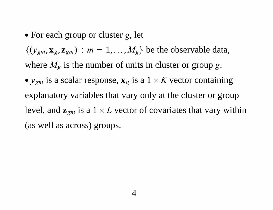
∙ For each group or cluster g, letygm,xg,zgm : m 1, . . . ,Mg be the observable data,
where Mg is the number of units in cluster or group g.
∙ ygm is a scalar response, xg is a 1 K vector containing
explanatory variables that vary only at the cluster or grouplevel, and zgm is a 1 L vector of covariates that vary within
(as well as across) groups.
4
∙Without a cluster identifier, a cluster sample looks like across section data set. Statistically, the difference is thatclusters, not individuals, have been drawn.∙ The clusters are assumed to be independent of each other,but outcomes within a cluster should be allowed to becorrelated.
5
∙ Linear model with additive error:
ygm xg zgm vgm
for m 1, . . . ,Mg, g 1, . . . ,G.
∙ Key questions:(1) Are we primarily interested in (group-level
coefficients) or (individual-level coefficients)?
6

(2) Does vgm contain a common group effect, as in
vgm cg ugm,m 1, . . . ,Mg,
where cg is an unobserved group (cluster) effect and ugm is
the idiosyncratic component? (Act as if it does.)(3) Are the regressors xg,zgm appropriately exogenous?
(4) How big are the group sizes (Mg) and number of groups
(G)? For now, we are assuming “large” G and “small”Mg,
but we cannot give specific values.
7
Pooled OLS Estimation∙ The theory with G → and fixed group sizes, Mg, is well
developed [White (1984), Arellano (1987)].∙ If we assume
Evgm|xg,zgm 0
then pooled OLS estimator of ygm on
1,xg,zgm,m 1, . . . ,Mg; g 1, . . . ,G, is consistent for
≡ ,′,′′ (as G → with Mg fixed) and and
G -asymptotically normal.
8

∙ Robust variance matrix is needed to account for correlationwithin clusters.∙Write Wg as the Mg 1 K L matrix of all regressors
for group g.∙ Estimator:
∑g1
G
Wg′ Wg
−1
∑g1
G
Wg′ vgvg′ Wg ∑
g1
G
Wg′ Wg
−1
,
where vg is the Mg 1 vector of pooled OLS residuals for
group g.
9

∙ This “sandwich” estimator is now computed routinelyusing “cluster” options.∙ Sometimes an adjustment is made, such as multiplying byG/G − 1.∙ These standard errors are robust to heteroskedasticity.∙ Structure of asymptotic variance is identical to panel datacase (G N, Mg T).
∙ Cluster samples are usually “unbalanced” (Mg vary across
g).
10
Random Effects Estimation∙ GLS: Strengthen the exogeneity assumption to
Evgm|xg,Zg 0,m 1, . . . ,Mg;g 1, . . . ,G,
where Zg is the Mg L matrix of unit-specific covariates.
∙ “Strict exogeneity” for cluster samples (without a timedimension).∙ Correlation of zgm with ugr violates the assumption. Might
want to include peer effects.
11
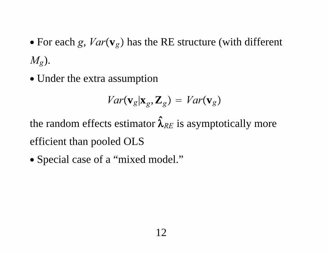
∙ For each g, Varvg has the RE structure (with different
Mg).
∙ Under the extra assumption
Varvg|xg,Zg Varvg
the random effects estimator RE is asymptotically moreefficient than pooled OLS∙ Special case of a “mixed model.”
12

∙ Important point: One can, and probably should, make REinference robust to an unknown form of Varvg|xg,Zg,
even though there is no time dimension (serial correlation).∙ The RE estimator may be more efficient than OLS even ifVarvg|xg,Zg does not have the RE structure.
13
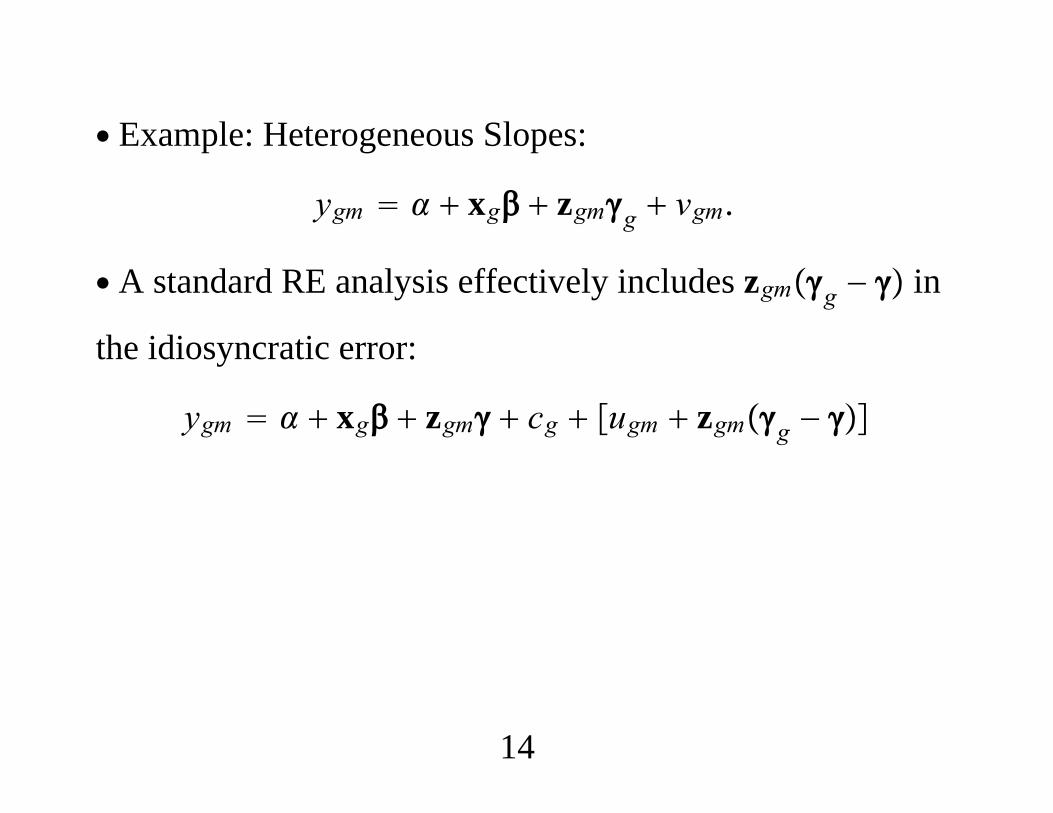
∙ Example: Heterogeneous Slopes:
ygm xg zgmg vgm.
∙ A standard RE analysis effectively includes zgmg − in
the idiosyncratic error:
ygm xg zgm cg ugm zgmg −
14
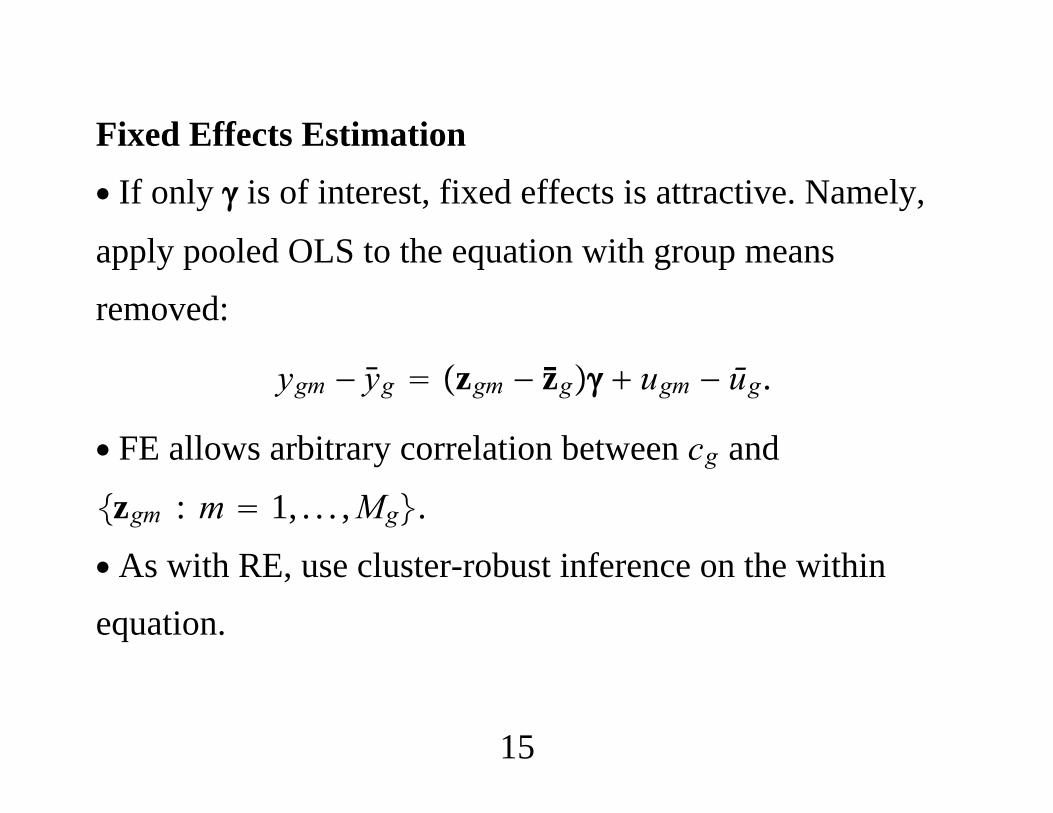
Fixed Effects Estimation∙ If only is of interest, fixed effects is attractive. Namely,
apply pooled OLS to the equation with group meansremoved:
ygm − yg zgm − zg ugm − ūg.
∙ FE allows arbitrary correlation between cg and
zgm : m 1, . . . ,Mg.
∙ As with RE, use cluster-robust inference on the withinequation.
15
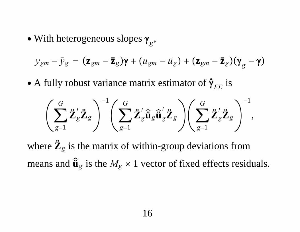
∙With heterogeneous slopes g,
ygm − yg zgm − zg ugm − ūg zgm − zgg −
∙ A fully robust variance matrix estimator of FE is
∑g1
G
Zg′ Zg
−1
∑g1
G
Zg′ üg
üg′Zg ∑
g1
G
Zg′ Zg
−1
,
where Zg is the matrix of within-group deviations from
means andüg is the Mg 1 vector of fixed effects residuals.
16
∙ Can also use the regression-based Hausman test forcomparing RE and FE: Pooled OLS or RE on
ygm xg zgm zg egm,
and test H0 : 0 using cluster-robust robust inference.
∙ POLS and RE are identical and both give the FE estimateof [Wooldridge (2009)].
17

∙ Example: Salary-Benefits Tradeoff for Elementary SchoolTeachers in Michigan.∙ Assumes the sampling was done at the school districtlevel. Units are schools within a district.
18

. des
Contains data from C:\mitbook1_2e\statafiles\benefits.dtaobs: 1,848
distid float %9.0g district identifierschid int %9.0g school identifierlunch float %9.0g percent eligible, free lunchenroll int %9.0g school enrollmentstaff float %9.0g staff per 1000 studentsexppp int %9.0g expenditures per pupilavgsal float %9.0g average teacher salary, $avgben int %9.0g average teacher non-salary
benefits, $math4 float %9.0g percent passing 4th grade math
testbs float %9.0g avgben/avgsallavgsal float %9.0g log(avgsal)lenroll float %9.0g log(enroll)lstaff float %9.0g log(staff)----------------------------------------------------------------------------Sorted by: distid schid
19

. reg lavgsal bs lstaff lenroll lunch
Source | SS df MS Number of obs 1848------------------------------------------- F( 4, 1843) 429.
Model | 48.3485452 4 12.0871363 Prob F 0.0000Residual | 51.8328336 1843 .028124164 R-squared 0.4826
------------------------------------------- Adj R-squared 0.4815Total | 100.181379 1847 .054240054 Root MSE .1677
----------------------------------------------------------------------------lavgsal | Coef. Std. Err. t P|t| [95% Conf. Interval
---------------------------------------------------------------------------bs | -.1774396 .1219691 -1.45 0.146 -.4166518 .0617725
lstaff | -.6907025 .0184598 -37.42 0.000 -.7269068 -.6544981lenroll | -.0292406 .0084997 -3.44 0.001 -.0459107 -.0125705
lunch | -.0008471 .0001625 -5.21 0.000 -.0011658 -.0005284_cons | 13.72361 .1121095 122.41 0.000 13.50374 13.94349
----------------------------------------------------------------------------
20
. reg lavgsal bs lstaff lenroll lunch, cluster(distid)
(Std. Err. adjusted for 537 clusters in distid----------------------------------------------------------------------------
| Robustlavgsal | Coef. Std. Err. t P|t| [95% Conf. Interval
---------------------------------------------------------------------------bs | -.1774396 .2596214 -0.68 0.495 -.6874398 .3325605
lstaff | -.6907025 .0352962 -19.57 0.000 -.7600383 -.6213666lenroll | -.0292406 .0257414 -1.14 0.256 -.079807 .0213258
lunch | -.0008471 .0005709 -1.48 0.138 -.0019686 .0002744_cons | 13.72361 .2562909 53.55 0.000 13.22016 14.22707
----------------------------------------------------------------------------
21
. xtreg lavgsal bs lstaff lenroll lunch, re
Random-effects GLS regression Number of obs 1848Group variable: distid Number of groups 537
R-sq: within 0.5453 Obs per group: min between 0.3852 avg 3overall 0.4671 max 162
----------------------------------------------------------------------------lavgsal | Coef. Std. Err. z P|z| [95% Conf. Interval
---------------------------------------------------------------------------bs | -.3812698 .1118678 -3.41 0.001 -.6005267 -.162013
lstaff | -.6174177 .0153587 -40.20 0.000 -.6475202 -.5873151lenroll | -.0249189 .0075532 -3.30 0.001 -.0397228 -.0101149
lunch | .0002995 .0001794 1.67 0.095 -.0000521 .0006511_cons | 13.36682 .0975734 136.99 0.000 13.17558 13.55806
---------------------------------------------------------------------------sigma_u | .12627558sigma_e | .09996638
rho | .61473634 (fraction of variance due to u_i)----------------------------------------------------------------------------
22

. xtreg lavgsal bs lstaff lenroll lunch, re cluster(distid)
Random-effects GLS regression Number of obs 1848Group variable: distid Number of groups 537
(Std. Err. adjusted for 537 clusters in distid----------------------------------------------------------------------------
| Robustlavgsal | Coef. Std. Err. z P|z| [95% Conf. Interval
---------------------------------------------------------------------------bs | -.3812698 .1504893 -2.53 0.011 -.6762235 -.0863162
lstaff | -.6174177 .0363789 -16.97 0.000 -.688719 -.5461163lenroll | -.0249189 .0115371 -2.16 0.031 -.0475312 -.0023065
lunch | .0002995 .0001963 1.53 0.127 -.0000852 .0006841_cons | 13.36682 .1968713 67.90 0.000 12.98096 13.75268
---------------------------------------------------------------------------sigma_u | .12627558sigma_e | .09996638
rho | .61473634 (fraction of variance due to u_i)----------------------------------------------------------------------------
23

. xtreg lavgsal bs lstaff lenroll lunch, fe
Fixed-effects (within) regression Number of obs 1848Group variable: distid Number of groups 537
----------------------------------------------------------------------------lavgsal | Coef. Std. Err. t P|t| [95% Conf. Interval
---------------------------------------------------------------------------bs | -.4948449 .133039 -3.72 0.000 -.7558382 -.2338515
lstaff | -.6218901 .0167565 -37.11 0.000 -.6547627 -.5890175lenroll | -.0515063 .0094004 -5.48 0.000 -.0699478 -.0330648
lunch | .0005138 .0002088 2.46 0.014 .0001042 .0009234_cons | 13.61783 .1133406 120.15 0.000 13.39548 13.84018
---------------------------------------------------------------------------sigma_u | .15491886sigma_e | .09996638
rho | .70602068 (fraction of variance due to u_i)----------------------------------------------------------------------------F test that all u_i0: F(536, 1307) 7.24 Prob F 0.0000
24
. xtreg lavgsal bs lstaff lenroll lunch, fe cluster(distid)
Fixed-effects (within) regression Number of obs 1848Group variable: distid Number of groups 537
(Std. Err. adjusted for 537 clusters in distid----------------------------------------------------------------------------
| Robustlavgsal | Coef. Std. Err. t P|t| [95% Conf. Interval
---------------------------------------------------------------------------bs | -.4948449 .1937316 -2.55 0.011 -.8754112 -.1142785
lstaff | -.6218901 .0431812 -14.40 0.000 -.7067152 -.5370649lenroll | -.0515063 .0130887 -3.94 0.000 -.0772178 -.0257948
lunch | .0005138 .0002127 2.42 0.016 .0000959 .0009317_cons | 13.61783 .2413169 56.43 0.000 13.14379 14.09187
---------------------------------------------------------------------------sigma_u | .15491886sigma_e | .09996638
rho | .70602068 (fraction of variance due to u_i)----------------------------------------------------------------------------
25

. * Create within-district means of all covariates.
. egen bsbar mean(bs), by(distid)
. egen lstaffbar mean(lstaff), by(distid)
. egen lenrollbar mean(lenroll), by(distid)
. egen lunchbar mean(lunch), by(distid)
26

. xtreg lavgsal bs lstaff lenroll lunch bsbar lstaffbar lenrollbar lunchbar,re cluster(distid)
Random-effects GLS regression Number of obs 1848Group variable: distid Number of groups 537
(Std. Err. adjusted for 537 clusters in distid----------------------------------------------------------------------------
| Robustlavgsal | Coef. Std. Err. z P|z| [95% Conf. Interval
---------------------------------------------------------------------------bs | -.4948449 .1939422 -2.55 0.011 -.8749646 -.1147252
lstaff | -.6218901 .0432281 -14.39 0.000 -.7066157 -.5371645lenroll | -.0515063 .013103 -3.93 0.000 -.0771876 -.025825
lunch | .0005138 .000213 2.41 0.016 .0000964 .0009312bsbar | .2998553 .3031961 0.99 0.323 -.2943981 .8941088
lstaffbar | -.0255493 .0651932 -0.39 0.695 -.1533256 .1022269lenrollbar | .0657285 .020655 3.18 0.001 .0252455 .1062116
lunchbar | -.0007259 .0004378 -1.66 0.097 -.0015839 .0001322_cons | 13.22003 .2556139 51.72 0.000 12.71904 13.72103
---------------------------------------------------------------------------
27

. test bsbar lstaffbar lenrollbar lunchbar
( 1) bsbar 0( 2) lstaffbar 0( 3) lenrollbar 0( 4) lunchbar 0
chi2( 4) 20.70Prob chi2 0.0004
28
2. Cluster-Robust Inference with Large GroupSizes∙What if one applies robust inference when the fixedMg,
G → asymptotic analysis is not realistic?∙ Hansen (2007): With G and Mg both getting large, the
usual inference based on the cluster-robust robust estimatoris valid with arbitrary within-group correlation among thevgm. (Independence across groups is maintained.)
29
∙ For example, if we have a sample of G 100 schools androughly Mg 100 students per school cluster-robust
inference for pooled OLS should produce inference ofroughly the correct size.
30
∙ The presence of cluster effects with a small number ofgroups (G) and large group sizes (Mg), cluster-robust
inference with pooled OLS falls outside Hansen’s theoreticalfindings.∙ Cameron, Gelbach, and Miller (2008) find that clusteringcan work well with G as small as five, and especiallyG ≥ 10.
31
∙ Usual “pairs cluster” bootstrap works less well thanresidual-based bootstrap.∙ Bootstrapping the t statistic works better thanbootstrapping the standard error. (Asymptotic refinement.)
32

∙ If the explanatory variables of interest vary within group,FE is attractive.1. Allows cg to be arbitrarily correlated with the zgm.
2. With largeMg, can treat the cg as parameters to estimate,
and then assume that the observations are independentacross m (as well as g). Usual inference, perhaps maderobust to heteroskedasticity, is valid.
33

3. Ex Post Clustering of a Random Sample∙ Growing use of clustered standard errors after randomsampling from a large population. “Ex post clustering.”∙ County, state, occupation, industry.∙ Even with heterogeneity across groups, no need to cluster.It can be very conservative.
34
∙ Abadie, Imbens, Wooldridge (in progress).∙ Suppose fourth graders are randomly sampled fromMichigan. For each student we learn their school, schooldistrict, intermediate school district. At which level shouldwe cluster?∙ Answer: We should not cluster at all.∙ Ex post clustering induces within-group correlation thatblows up standard errors.
35

∙ Consider estimating the mean, , from a population.
Randomly draw N observations.∙ There are G groups and the within-group means areheterogeneous.∙ The usual standard error is valid.∙ If we cluster, we compute the variance estimator
GG − 1 N−2 ∑
i1
N
êi2 ∑i1
N
∑h≠i
N
∑g1
G
sigshgêiêh
36

∙ The sig are the group indicators, collect along with
yi ei.
∙ Can show that, replacing êi yi − y with ei, the expectedvalue is
GG − 1
e2N N − 1
N 2
2 ≡ ∑g1
G
g2g2 ≥ 0
g Psig 1, g Eei|sig 1
37
∙ Formula works well in simulations, for both small andlarge G.∙ Similar result can be shown for regression.∙ Important: The clustering produces upward biasedvariances even if the covariate is fixed at the group level.For example, xg 1 if school g is a charter school, zero
otherwise.
38

∙ Caveat: Sampling experiment is that the group feature isfixed and then we repeatedly sample individual units. So, ata point in time, some schools are charter schools and someare not. Some states are right-to-work, others are not.
39
∙ Two cases where clustering an initial random sample isneeded:1. The group-level variable, xg, is reassigned with the
random draws of individuals.2. A group-level variable, such as an average, is used in theanalysis. For example, peer effects computed at the schoollevel. (Contrast school-level poverty rates known fromadministrative records and a poverty rate computed afterrandom sampling.)
40

∙ Claims hold whether we use pooled OLS or add groupindicators (group “fixed effects”).Simulations∙ Findings hold with infinite population and randomsampling or random sampling (without replacement) from afinite population.∙ Following are finite population, 10 percent randomsampling.∙ Heterogeneity in population.∙ N 10,000, G 50, H 10.
41
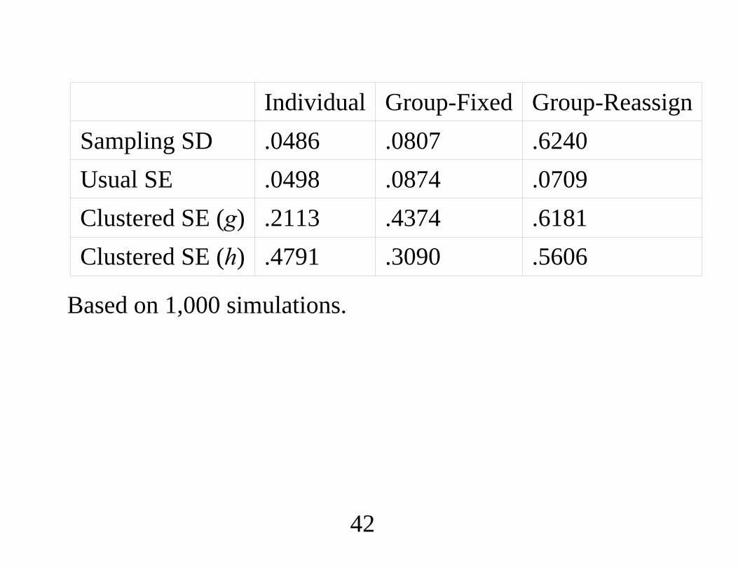
Individual Group-Fixed Group-ReassignSampling SD .0486 .0807 .6240Usual SE .0498 .0874 .0709Clustered SE (g) .2113 .4374 .6181Clustered SE (h) .4791 .3090 .5606
Based on 1,000 simulations.
42
4. Cluster Samples with Unit-Specific Panel Data∙ Cluster samples can come with a time component, so thatthere are two potential sources of correlation acrossobservations: across time within the same individual andacross individuals within the same group.∙ Assume there is a natural nesting. Each unit belongs to acluster and the cluster identification does not change overtime.
43

∙ For example, we might have annual panel data at the firmlevel, and each firm belongs to the same industry (cluster)for all years.∙ Or, we have panel data for schools that each belong to adistrict.∙ The sampling is done at the higher level.
44
∙ Have three data subscripts on at least some variables thatwe observe. For example, the response variable is ygmt,
where g indexes the group or cluster, m is the unit within thegroup, and t is the time index.∙ Assume we have a balanced panel with the time periodsrunning from t 1, . . . ,T.
45

∙We assume that we have many groups, G, and relativelyfew members of the group.∙ Asymptotics: fixed Mg and T fixed with G getting large.
∙ For example, we sample several hundred school districtswith a few to maybe a few dozen schools per district, over ahandful of years.∙ Hansen’s (2007) results apply for small T but where Mg is
also “large.”
46
∙ One example of a linear model with constant slopes:
ygmt t wg xgm zgmt hg cgm ugmt,
where, say, hg is the district effect, cgm is the school effect
(school m in district g), and ugmt is the idiosyncratic effect.
∙ The composite error is
vgmt hg cgm ugmt.
47
∙ The model can include variables that change at any level.∙ Some elements of zgmt might change only across g and t,
and not by unit.∙With the presence of wg, or variables that change across g
and t, need to recognize hg.
48
∙ If assume the error vgmt is uncorrelated with
wg,xgm,zgmt, pooled OLS is simple and attractive.
Consistent as G → for any cluster or serial correlationpattern.∙ The most general inference for pooled OLS – stillmaintaining independence across clusters – is to allow anykind of serial correlation across units or time, or both, withina cluster.
49
∙ In Stata:reg y w1 ... wJ x1 ... xK z1 ... zL,
cluster(districtid)
∙ Compare with inference robust only to serial correlation:reg y w1 ... wJ x1 ... xK z1 ... zL,
cluster(schoolid)
50
∙ In the context of cluster sampling with panel data, thelatter is no longer “fully robust” because it ignores possiblewithin-cluster correlation.
51
Generalized Least Squares∙ Can apply a generalized least squares analysis that makesassumptions about the components of the composite error.∙ Typically, assume components are pairwise uncorrelated,the cgm are uncorrelated within cluster (with common
variance), and the ugmt are uncorrelated within cluster and
across time (with common variance).
52
∙ Resulting feasible GLS estimator is an extension of theusual random effects estimator for panel data.∙ To guard against heteroskedasticity in any of the errors andserial correlation in the ugmt, one should use fully robust
inference that does not rely on the form of the unconditionalvariance matrix.∙ In Stata, command is xtmixed. Current version now
allows robust inference.
53

∙ Simpler strategy: apply random effects at the individuallevel, effectively ignoring the clusters in estimation. In otherwords, treat the data as a standard panel data set inestimation and apply usual RE. To account for the clustersampling in inference, one computes a fully robust variancematrix estimator for the usual random effects estimator.
54

∙ In Stata:xtset schoolid year
xtreg y w1 ... wJ x1 ... xK
z1 ... zL, re cluster(districtid)
55
∙We have available different versions of fixed effectsestimators.∙ Removing cluster averages eliminates hg; when wgt wg
for all t, wg is also eliminated. But the unit-specific effects,
cmg, are still part of the error term.
∙ If we are mainly interested in , the coefficients on thetime-varying variables zgmt, then removing cgm (along with
hg) is attractive. In other words, use a standard fixed effects
analysis at the individual level.
56
∙ Even if we use unit “fixed effects” – that is, we demean thedata at the unit level – we should still use inference robust toclustering at the aggregate level.∙ As with simpler models, neglected heterogeneous slopescan cause extra cluster correlation.
57

∙ Example: Effects of Funding on Student Performance. use meap94_98
. des
Contains data from meap94_98.dtaobs: 7,150
variable name type format label variable label----------------------------------------------------------------------------distid float %9.0g district identifierschid int %9.0g school identifierlunch float %9.0g % eligible for free lunchenrol int %9.0g number of studentsexppp int %9.0g expenditure per pupilmath4 float %9.0g % satisfactory, 4th grade math
testSorted by: schid year
58

. * egen tobs sum(1), by(schid)
. tab tobs if y98
number of |time |
periods | Freq. Percent Cum.-----------------------------------------------
3 | 487 29.28 29.284 | 254 15.27 44.565 | 922 55.44 100.00
-----------------------------------------------Total | 1,663 100.00
59
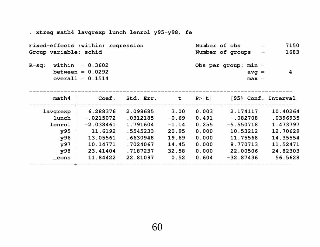
. xtreg math4 lavgrexp lunch lenrol y95-y98, fe
Fixed-effects (within) regression Number of obs 7150Group variable: schid Number of groups 1683
R-sq: within 0.3602 Obs per group: min between 0.0292 avg 4overall 0.1514 max
----------------------------------------------------------------------------math4 | Coef. Std. Err. t P|t| [95% Conf. Interval
---------------------------------------------------------------------------lavgrexp | 6.288376 2.098685 3.00 0.003 2.174117 10.40264
lunch | -.0215072 .0312185 -0.69 0.491 -.082708 .0396935lenrol | -2.038461 1.791604 -1.14 0.255 -5.550718 1.473797
y95 | 11.6192 .5545233 20.95 0.000 10.53212 12.70629y96 | 13.05561 .6630948 19.69 0.000 11.75568 14.35554y97 | 10.14771 .7024067 14.45 0.000 8.770713 11.52471y98 | 23.41404 .7187237 32.58 0.000 22.00506 24.82303
_cons | 11.84422 22.81097 0.52 0.604 -32.87436 56.5628---------------------------------------------------------------------------
60
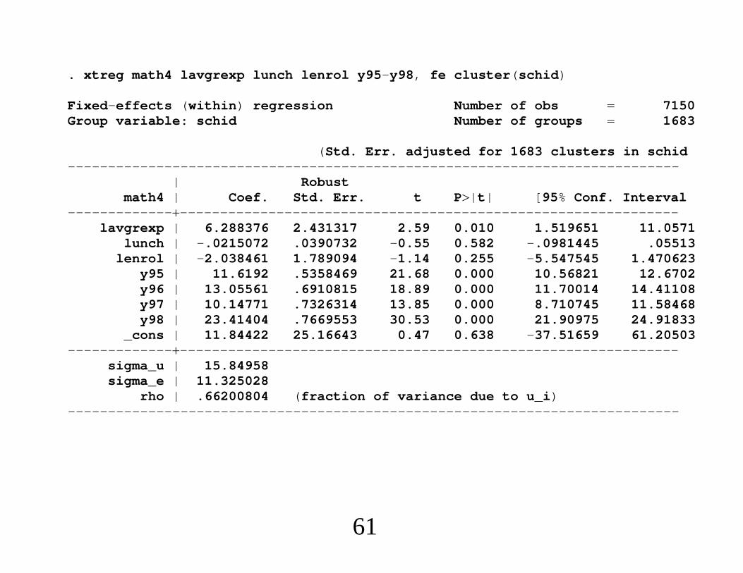
. xtreg math4 lavgrexp lunch lenrol y95-y98, fe cluster(schid)
Fixed-effects (within) regression Number of obs 7150Group variable: schid Number of groups 1683
(Std. Err. adjusted for 1683 clusters in schid----------------------------------------------------------------------------
| Robustmath4 | Coef. Std. Err. t P|t| [95% Conf. Interval
---------------------------------------------------------------------------lavgrexp | 6.288376 2.431317 2.59 0.010 1.519651 11.0571
lunch | -.0215072 .0390732 -0.55 0.582 -.0981445 .05513lenrol | -2.038461 1.789094 -1.14 0.255 -5.547545 1.470623
y95 | 11.6192 .5358469 21.68 0.000 10.56821 12.6702y96 | 13.05561 .6910815 18.89 0.000 11.70014 14.41108y97 | 10.14771 .7326314 13.85 0.000 8.710745 11.58468y98 | 23.41404 .7669553 30.53 0.000 21.90975 24.91833
_cons | 11.84422 25.16643 0.47 0.638 -37.51659 61.20503---------------------------------------------------------------------------
sigma_u | 15.84958sigma_e | 11.325028
rho | .66200804 (fraction of variance due to u_i)----------------------------------------------------------------------------
61

. xtreg math4 lavgrexp lunch lenrol y95-y98, fe cluster(distid)
(Std. Err. adjusted for 467 clusters in distid----------------------------------------------------------------------------
| Robustmath4 | Coef. Std. Err. t P|t| [95% Conf. Interval
---------------------------------------------------------------------------lavgrexp | 6.288376 3.132334 2.01 0.045 .1331271 12.44363
lunch | -.0215072 .0399206 -0.54 0.590 -.0999539 .0569395lenrol | -2.038461 2.098607 -0.97 0.332 -6.162365 2.085443
y95 | 11.6192 .7210398 16.11 0.000 10.20231 13.0361y96 | 13.05561 .9326851 14.00 0.000 11.22282 14.8884y97 | 10.14771 .9576417 10.60 0.000 8.26588 12.02954y98 | 23.41404 1.027313 22.79 0.000 21.3953 25.43278
_cons | 11.84422 32.68429 0.36 0.717 -52.38262 76.07107---------------------------------------------------------------------------
sigma_u | 15.84958sigma_e | 11.325028
rho | .66200804 (fraction of variance due to u_i)----------------------------------------------------------------------------
62

"Econometrics of Cross Section and Panel Data"
Lecture 8
Discrete Choice Models
Guido Imbens
Cemmap Lectures, UCL, June 2014

Outline
1. Introduction
2. Multinomial and Conditional Logit Models
3. Independence of Irrelevant Alternatives
4. Models without IIA
5. Berry-Levinsohn-Pakes
6. Models with Multiple Unobserved Choice Characteristics
7. Hedonic Models
1
1. Introduction
Various versions of multinomial logit models developed by Mc-
Fadden in 70’s.
In IO applications with substantial number of choices IIA prop-
erty found to be particularly unattractive because of unrealistic
implications for substitution patterns.
Random effects approach is more appealing generalization than
either nested logit or unrestricted multinomial probit
Generalization by BLP to allow for endogenous choice charac-
teristics, unobserved choice characteristics, using only aggre-
gate choice data.
2
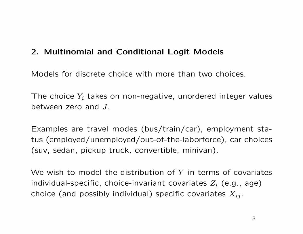
2. Multinomial and Conditional Logit Models
Models for discrete choice with more than two choices.
The choice Yi takes on non-negative, unordered integer values
between zero and J.
Examples are travel modes (bus/train/car), employment sta-
tus (employed/unemployed/out-of-the-laborforce), car choices
(suv, sedan, pickup truck, convertible, minivan).
We wish to model the distribution of Y in terms of covariates
individual-specific, choice-invariant covariates Zi (e.g., age)
choice (and possibly individual) specific covariates Xij.
3
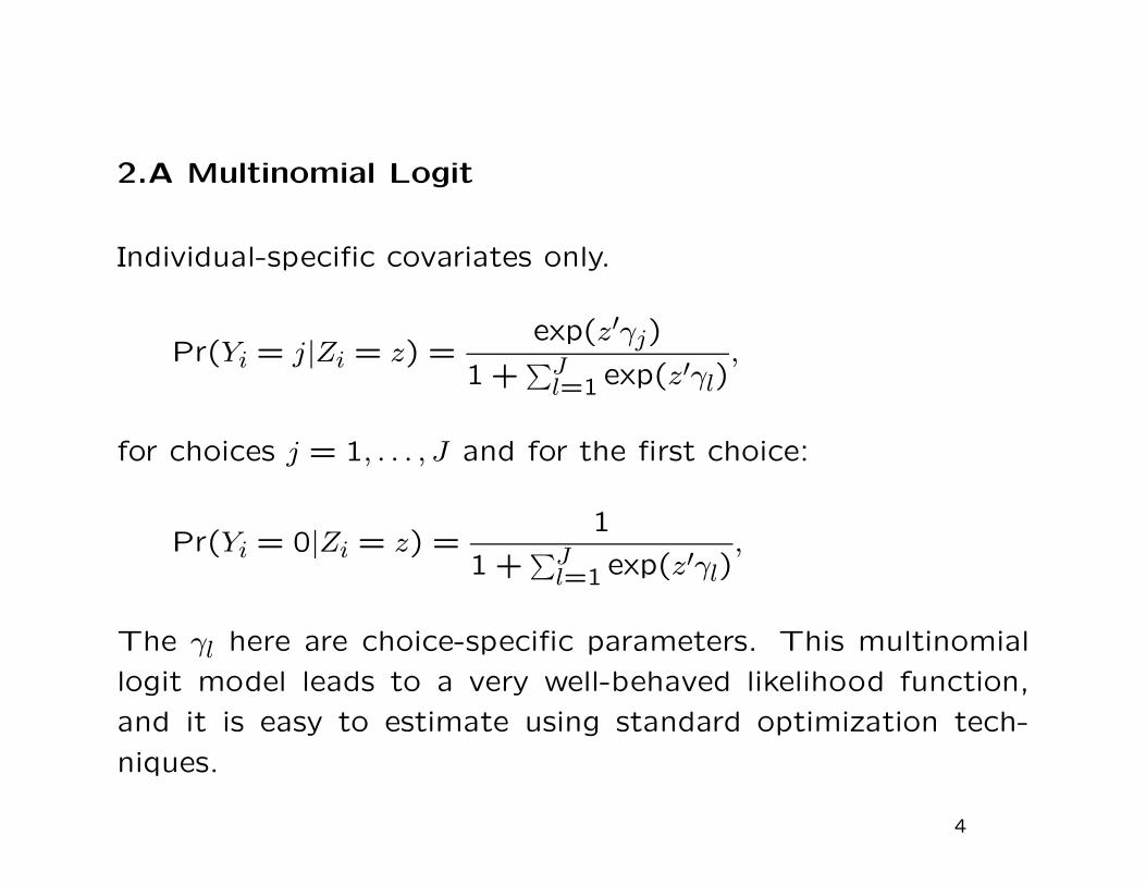
2.A Multinomial Logit
Individual-specific covariates only.
Pr(Yi = j|Zi = z) =exp(z′γj)
1 +∑J
l=1 exp(z′γl),
for choices j = 1, . . . , J and for the first choice:
Pr(Yi = 0|Zi = z) =1
1 +∑J
l=1 exp(z′γl),
The γl here are choice-specific parameters. This multinomial
logit model leads to a very well-behaved likelihood function,
and it is easy to estimate using standard optimization tech-
niques.
4
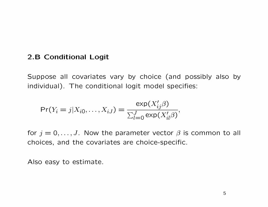
2.B Conditional Logit
Suppose all covariates vary by choice (and possibly also by
individual). The conditional logit model specifies:
Pr(Yi = j|Xi0, . . . , XiJ) =exp(X′
ijβ)∑J
l=0 exp(X′ilβ)
,
for j = 0, . . . , J. Now the parameter vector β is common to all
choices, and the covariates are choice-specific.
Also easy to estimate.
5

The multinomial logit model can be viewed as a special case
of the conditional logit model. Suppose we have a vector of
individual characteristics Zi of dimension K, and J vectors of
coefficients γj, each of dimension K. Then define
Xi1 =
Zi0......0
, . . . . . . XiJ =
0......0Zi
, and Xi0 =
0...0...0
,
and define the parameter vector as β = (γ′1, . . . , γ′
J)′. Then
Pr(Yi = j|Zi) =exp(Z′
iγj)
1 +∑J
k=1 exp(Z′iγk)
=exp(X′
ijβ)∑J
k=0 exp(X′ikβ)
= Pr(Yi = j|Xi0, . . . , XiJ)
6
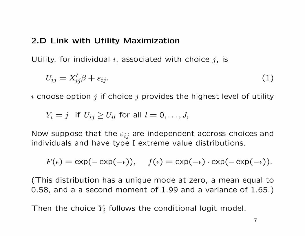
2.D Link with Utility Maximization
Utility, for individual i, associated with choice j, is
Uij = X′ijβ + εij. (1)
i choose option j if choice j provides the highest level of utility
Yi = j if Uij ≥ Uil for all l = 0, . . . , J,
Now suppose that the εij are independent accross choices and
individuals and have type I extreme value distributions.
F (ε) = exp(− exp(−ε)), f(ε) = exp(−ε) · exp(− exp(−ε)).
(This distribution has a unique mode at zero, a mean equal to
0.58, and a a second moment of 1.99 and a variance of 1.65.)
Then the choice Yi follows the conditional logit model.
7
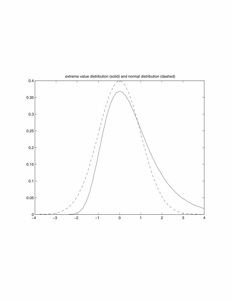
−4 −3 −2 −1 0 1 2 3 40
0.05
0.1
0.15
0.2
0.25
0.3
0.35
0.4extreme value distribution (solid) and normal distribution (dashed)
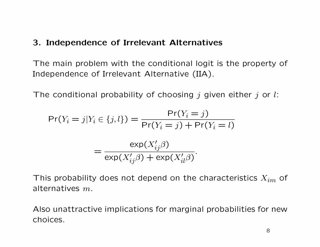
3. Independence of Irrelevant Alternatives
The main problem with the conditional logit is the property of
Independence of Irrelevant Alternative (IIA).
The conditional probability of choosing j given either j or l:
Pr(Yi = j|Yi ∈ j, l) =Pr(Yi = j)
Pr(Yi = j) + Pr(Yi = l)
=exp(X′
ijβ)
exp(X′ijβ) + exp(X′
ilβ).
This probability does not depend on the characteristics Xim of
alternatives m.
Also unattractive implications for marginal probabilities for new
choices.
8

Although multinomial and conditional logit models may fit well,
they are not necessarily attractive as behavior/structural mod-
els. because they generates unrealistic substitution patterns.
Suppose that individuals have the choice out of three restau-
rants, Chez Panisse (C), Lalime’s (L), and the Bongo Burger
(B). Suppose we have two characteristics, price and quality
price PC = 95, PL = 80, PB = 5,
quality QC = 10, QL = 9, QB = 2
market share SC = 0.10, SL = 0.25, SB = 0.65.
These numbers are roughly consistent with a conditional logit
model where the utility associated with individual i and restau-
rant j is
Uij = −0.2 · Pj + 2 · Qj + εij ,
9
Now suppose that we raise the price at Lalime’s to 1000 (or
raise it to infinity, corresponding to taking it out of business).
The conditional logit model predicts that the market share for
Lalime’s gets divided by Chez Panisse and the Bongo Burger,
proportional to their original market share, and thus SC = 0.13
and SB = 0.87: most of the individuals who would have gone
to Lalime’s will now dine (if that is the right term) at the
Bongo Burger.
That seems implausible. The people who were planning to
go to Lalime’s would appear to be more likely to go to Chez
Panisse if Lalime’s is closed than to go to the Bongo Burger,
implying SC ≈ 0.35 and SB ≈ 0.65.
10
Recall the latent utility set up with the utility
Uij = X′ijβ + εij. (2)
In the conditional logit model we assume independent extreme
value εij. The independence is essentially what creates the
IIA property. (This is not completely correct, because other
distributions for the unobserved, say with normal errors, we
would not get IIA exactly, but something pretty close to it.)
The solution is to allow in some fashion for correlation between
the unobserved components in the latent utility representation.
In particular, with a choice set that contains multiple versions
of similar choices (like Chez Panisse and LaLime’s), we should
allow the latent utilities for these choices to be similar.
11
4. Models without IIA
Here we discuss 3 ways of avoiding the IIA property. All can
be interpreted as relaxing the independence between the εij.
The first is the nested logit model where the researcher groups
together sets of choices. This allows for non-zero correlation
between unobserved components of choices within a nest and
maintains zero correlation across nests.
Second, the unrestricted multinomial probit model with no re-
strictions on the covariance between unobserved components,
beyond normalizations.
Third, the mixed or random coefficients logit where the marginal
utilities associated with choice characteristics vary between
individuals, generating positive correlation between the un-
observed components of choices that are similar in observed
choice characteristics.
12
Nested Logit Models
Partition the set of choices 0,1, . . . , J into S sets B1, . . . , BS
Now let the conditional probability of choice j given that your
choice is in the set Bs, be equal to
Pr(Yi = j|Xi, Yi ∈ Bs) =exp(ρ−1
s X′ijβ)
∑l∈Bs exp(ρ
−1s X′
ilβ),
for j ∈ Bs, and zero otherwise. In addition suppose the marginal
probability of a choice in the set Bs is
Pr(Yi ∈ Bs|Xi) =
(∑l∈Bs exp(ρ
−1s X′
ilβ))ρs
∑St=1
(∑l∈Bt
exp(ρ−1t X′
ilβ))ρs .
13

If we fix ρs = 1 for all s, then
Pr(Yi = j|Xi) =exp(X′
ijβ)∑S
t=1
∑l∈Bt
exp(X′ilβ)
,
and we are back in the conditional logit model.
The implied joint distribution function of the εij is
F (εi0, . . . , εiJ) = exp
−
S∑
s=1
∑
j∈Bs
exp(−ρ−1
s εij)
ρs .
Within the sets the correlation coefficient for the εij is approxi-
mately equal to 1−ρ. Between the sets the εij are independent.
The nested logit model could capture the restaurant example
by having two nests, the first B1 = Chez Panisse,LaLime′s,
and the second one B2 = Bongoburger.
14
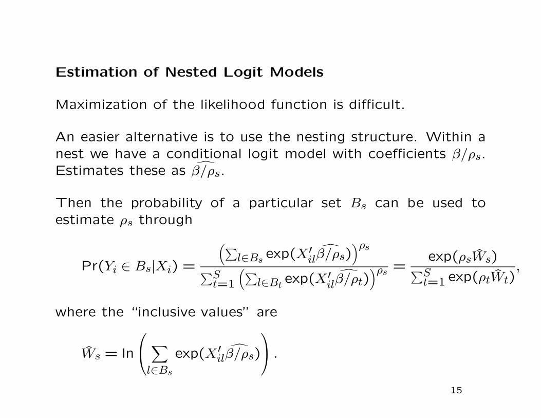
Estimation of Nested Logit Models
Maximization of the likelihood function is difficult.
An easier alternative is to use the nesting structure. Within a
nest we have a conditional logit model with coefficients β/ρs.
Estimates these as β/ρs.
Then the probability of a particular set Bs can be used to
estimate ρs through
Pr(Yi ∈ Bs|Xi) =
(∑l∈Bs exp(X′
ilβ/ρs))ρs
∑St=1
(∑l∈Bt
exp(X′ilβ/ρt)
)ρs =exp(ρsWs)
∑St=1 exp(ρtWt)
,
where the “inclusive values” are
Ws = ln
∑
l∈Bs
exp(X′ilβ/ρs)
.
15

These models can be extended to many layers of nests. See
for an impressive example of a complex model with four layers
of multiple nests Goldberg (1995). Figure 2 shows the nests
in the Goldberg application.
The key concern with the nested logit models is that results
may be sensitive to the specification of the nest structure.
The researcher chooses which choices are potentially close
substitutes, with the data being used to estimate the amount
of correlation.
Researcher would have to choose nest for new good to estimate
market share.
16
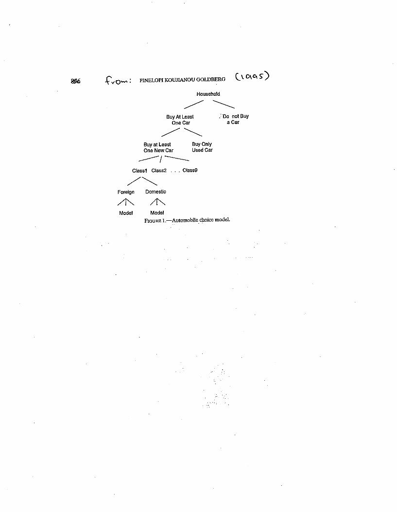

Multinomial Probit with Unrestricted Covariance Matrix
A second possibility is to directly free up the covariance matrix
of the error terms. This is more natural to do in the multino-
mial probit case.
We specify:
Ui =
Ui0Ui1...
UiJ
=
X′i0β + εi0
X′i1β + εi1
...X′
iJβ + εiJ
εi =
εi0εi1...
εiJ
|Xi ∼ N(0,Ω),
for some relatively unrestricted (J + 1) × (J + 1) covariance
matrix Ω (beyond normalizations).
17
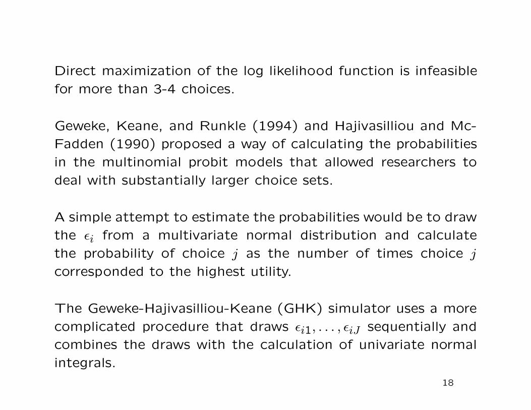
Direct maximization of the log likelihood function is infeasible
for more than 3-4 choices.
Geweke, Keane, and Runkle (1994) and Hajivasilliou and Mc-
Fadden (1990) proposed a way of calculating the probabilities
in the multinomial probit models that allowed researchers to
deal with substantially larger choice sets.
A simple attempt to estimate the probabilities would be to draw
the εi from a multivariate normal distribution and calculate
the probability of choice j as the number of times choice j
corresponded to the highest utility.
The Geweke-Hajivasilliou-Keane (GHK) simulator uses a more
complicated procedure that draws εi1, . . . , εiJ sequentially and
combines the draws with the calculation of univariate normal
integrals.
18

From a Bayesian perspective drawing from the posterior dis-
tribution of β and Ω is straightforward. The key is setting up
the vector of unobserved random variables as
θ = (β,Ω, Ui0, . . . , UiJ) ,
and defining the most convenient partition of this vector.
Suppose we know the latent utilities Ui for all individuals. Then
the normality makes this a standard linear model problem.
Given the parameters drawing from the unobserved utilities
can be done sequentially: for each unobserved utility given
the others we would have to draw from a truncated normal
distribution, which is straightforward. See McCulloch, Polson,
and Rossi (2000) for details.
19

Merits of Unrestriced Multinomial Probit
The attraction of this approach is that there are no restrictions
on which choices are close substitutes.
The difficulty, however, with the unrestricted multinomial pro-
bit approach is that with a reasonable number of choices there
are a large number of parameters: all elements in the (J +
1) × (J + 1) dimensional Ω minus some normalizations and
symmetry restrictions.
Estimating all these covariance parameters precisely, based on
only first choice data (as opposed to data where we know
for each individual additional orderings, e.g., first and second
choices), is difficult.
Prediction for new good would require specifying correlations
with all other goods.
20
Random Effects Models
A third possibility to get around the IIA property is to allow for
unobserved heterogeneity in the slope coefficients.
Why do we fundamentally think that if Lalime’s price goes
up, the individuals who were planning to go Lalime’s go to
Chez Panisse instead, rather than to the Bongo Burger? One
argument is that we think individuals who have a taste for
Lalime’s are likely to have a taste for close substitute in terms
of observable characteristics, Chez Panisse as well, rather than
for the Bongo Burger.
22

We can model this by allowing the marginal utilities to vary at
the individual level:
Uij = X′ijβi + εij,
We can also write this as
Uij = X′ijβ + νij,
where
νij = εij + Xij · (βi − β),
which is no longer independent across choices.
23
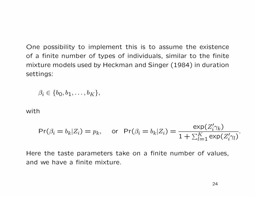
One possibility to implement this is to assume the existence
of a finite number of types of individuals, similar to the finite
mixture models used by Heckman and Singer (1984) in duration
settings:
βi ∈ b0, b1, . . . , bK,
with
Pr(βi = bk|Zi) = pk, or Pr(βi = bk|Zi) =exp(Z′
iγk)
1 +∑K
l=1 exp(Z′iγl)
.
Here the taste parameters take on a finite number of values,
and we have a finite mixture.
24
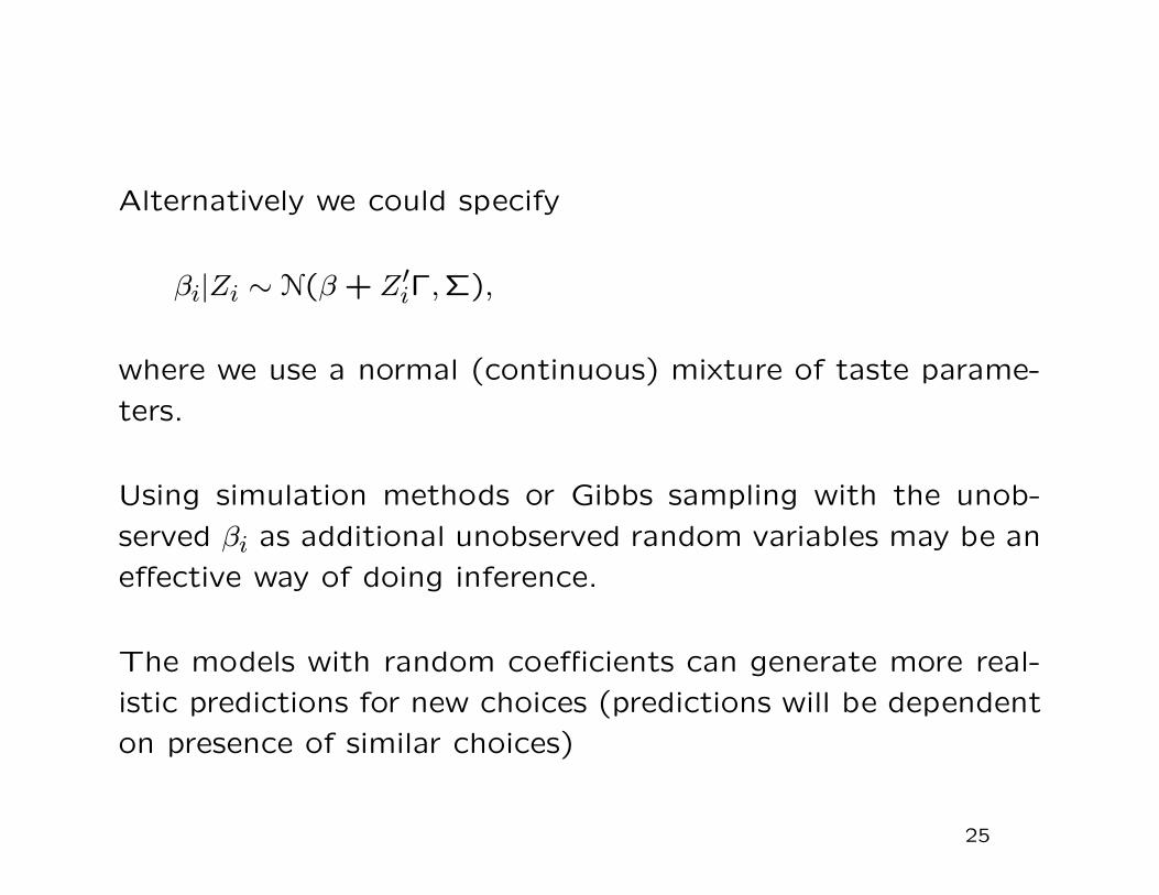
Alternatively we could specify
βi|Zi ∼ N(β + Z′iΓ,Σ),
where we use a normal (continuous) mixture of taste parame-
ters.
Using simulation methods or Gibbs sampling with the unob-
served βi as additional unobserved random variables may be an
effective way of doing inference.
The models with random coefficients can generate more real-
istic predictions for new choices (predictions will be dependent
on presence of similar choices)
25
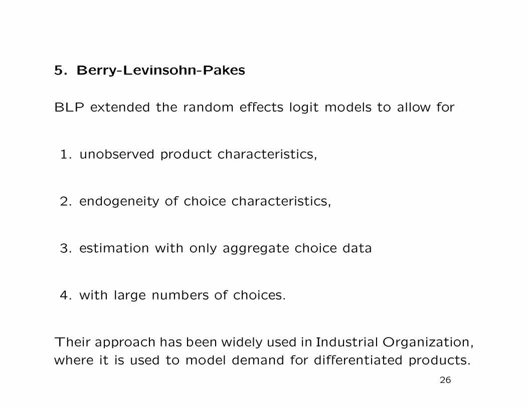
5. Berry-Levinsohn-Pakes
BLP extended the random effects logit models to allow for
1. unobserved product characteristics,
2. endogeneity of choice characteristics,
3. estimation with only aggregate choice data
4. with large numbers of choices.
Their approach has been widely used in Industrial Organization,
where it is used to model demand for differentiated products.
26
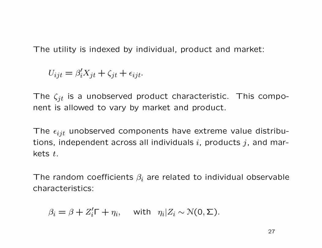
The utility is indexed by individual, product and market:
Uijt = β′iXjt + ζjt + εijt.
The ζjt is a unobserved product characteristic. This compo-
nent is allowed to vary by market and product.
The εijt unobserved components have extreme value distribu-
tions, independent across all individuals i, products j, and mar-
kets t.
The random coefficients βi are related to individual observable
characteristics:
βi = β + Z′iΓ + ηi, with ηi|Zi ∼ N(0,Σ).
27

The data consist of
• estimated shares stj for each choice j in each market t,
• observations from the marginal distribution of individual
characteristics (the Zi’s) for each market, often from rep-
resentative data sets such as the CPS.
First write the latent utilities as
Uijt = δjt + νijt + εijt,
where
δjt = β′Xjt + ζjt, and νijt = (Z′iΓ + ηi)
′Xjt.
28
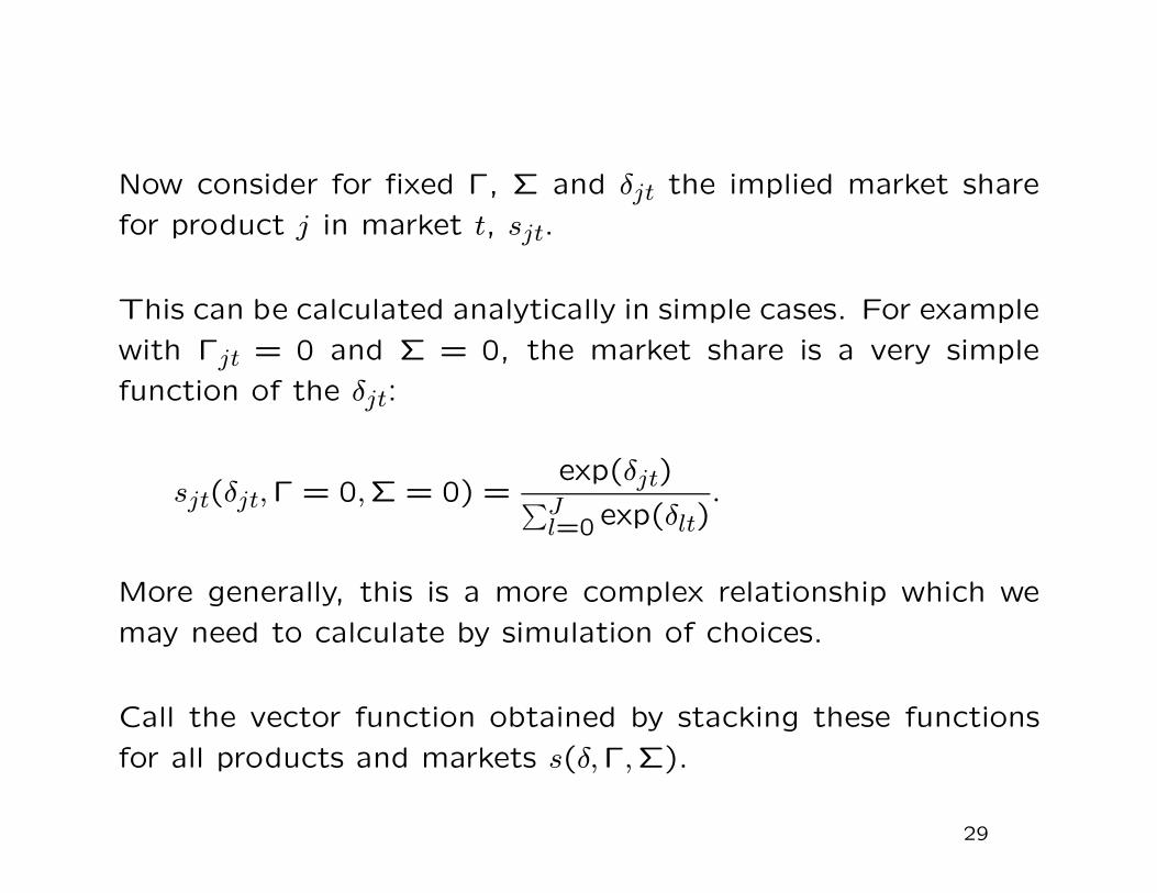
Now consider for fixed Γ, Σ and δjt the implied market share
for product j in market t, sjt.
This can be calculated analytically in simple cases. For example
with Γjt = 0 and Σ = 0, the market share is a very simple
function of the δjt:
sjt(δjt,Γ = 0,Σ = 0) =exp(δjt)∑J
l=0 exp(δlt).
More generally, this is a more complex relationship which we
may need to calculate by simulation of choices.
Call the vector function obtained by stacking these functions
for all products and markets s(δ,Γ,Σ).
29
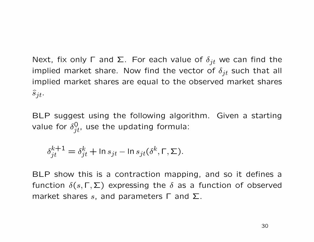
Next, fix only Γ and Σ. For each value of δjt we can find the
implied market share. Now find the vector of δjt such that all
implied market shares are equal to the observed market shares
sjt.
BLP suggest using the following algorithm. Given a starting
value for δ0jt, use the updating formula:
δk+1jt = δk
jt + ln sjt − ln sjt(δk,Γ,Σ).
BLP show this is a contraction mapping, and so it defines a
function δ(s,Γ,Σ) expressing the δ as a function of observed
market shares s, and parameters Γ and Σ.
30
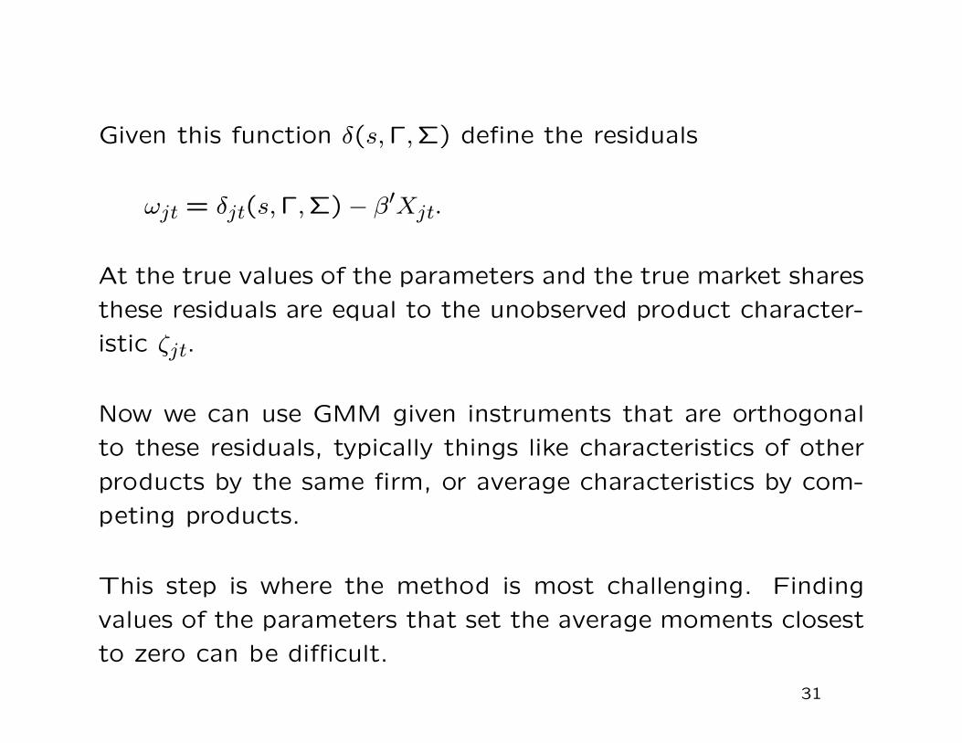
Given this function δ(s,Γ,Σ) define the residuals
ωjt = δjt(s,Γ,Σ) − β′Xjt.
At the true values of the parameters and the true market shares
these residuals are equal to the unobserved product character-
istic ζjt.
Now we can use GMM given instruments that are orthogonal
to these residuals, typically things like characteristics of other
products by the same firm, or average characteristics by com-
peting products.
This step is where the method is most challenging. Finding
values of the parameters that set the average moments closest
to zero can be difficult.
31
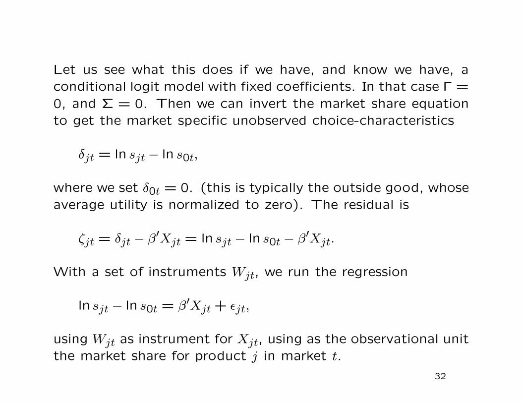
Let us see what this does if we have, and know we have, a
conditional logit model with fixed coefficients. In that case Γ =
0, and Σ = 0. Then we can invert the market share equation
to get the market specific unobserved choice-characteristics
δjt = ln sjt − ln s0t,
where we set δ0t = 0. (this is typically the outside good, whose
average utility is normalized to zero). The residual is
ζjt = δjt − β′Xjt = ln sjt − ln s0t − β′Xjt.
With a set of instruments Wjt, we run the regression
ln sjt − ln s0t = β′Xjt + εjt,
using Wjt as instrument for Xjt, using as the observational unit
the market share for product j in market t.
32
6. Models with Multiple Unobserved Choice Characteris-
tics
The BLP approach can allow only for a single unobserved
choice characteristic. This is essential for their estimation
strategy with aggregate data.
With individual level data one may be able to establish the
presence of two unobserved product characteristics (invariant
across markets). Elrod and Keane (1995), Goettler and Shachar
(2001), and Athey and Imbens (2007) study such models.
These models can be viewed as freeing up the covariance ma-
trix of unobserved components relative to the random coef-
ficients model, but using a factor structure instead of a fully
unrestricted covariance matrix as in the multinomial probit.
33
Athey and Imbens model the latent utility for individual i in
market t for choice j as
Uijt = X′itβi + ζ ′jγi + εijt,
with the individual-specific taste parameters for both the ob-
served and unobserved choice characteristics normally distributed:
(βiγi
)|Zi ∼ N(ΓZi,Σ).
Even in the case with all choice characteristics exogenous, max-
imum likelihood estimation would be difficult (multiple modes).
Bayesian methods, and in particular markov-chain-monte-carlo
methods are more effective tools for conducting inference in
these settings.
34
7. Hedonic Models
Recently researchers have reconsidered using pure characteris-
tics models for discrete choices, that is models with no idiosyn-
cratic error εij, instead relying solely on the presence of a small
number of unobserved product characteristics and unobserved
variation in taste parameters to generate stochastic choices.
Why can it still be useful to include such an εij?
35
First, the pure characteristics model can be extremely sensi-
tive to measurement error, because it can predict zero market
shares for some products.
Consider a case where choices are generated by a pure char-
acteristics model that implies that a particular choice j has
zero market share. Now suppose that there is a single unit i
for whom we observe, due to measurement error, the choice
Yi = j.
Irrespective of the number of correctly measured observations
available that were generated by the pure characteristics model,
the estimates of the latent utility function will not be close to
the true values due to a single mismeasured observation.
36

Thus, one might wish to generalize the model to be more
robust. One possibility is to related the observed choice Yi to
the optimal choice Y ∗i :
Pr(Yi = y|Y ∗i , Xi, νi, Z1, . . . , ZJ , ζ1, . . . , ζJ)
=
1 − δ if Y = Y ∗
i ,δ/(J − 1) if Y 6= Y ∗
i .
This nests the pure characteristics model (by setting δ = 0),
without the extreme sensitivity.
However, if the optimal choice Y ∗i is not observed, all of the
remaining choices are equally likely.
37

An alternative modification of the pure characteristics model
is based on adding an idiosyncratic error term to the utility
function. This model will have the feature that, conditional
on the optimal choice not being observed, a close-to-optimal
choice is more likely than a far-from-optimal choice.
Suppose the true utility is U∗ij but individuals base their choice
on the maximum of mismeasured version of this utility:
Uij = U∗ij + εij,
with an extreme value εij, independent across choices and in-
dividuals. The εij here can be interpreted as an error in the
calculation of the utility associated with a particular choice.
38
Second, this model approximately nests the pure characteristics
model in the following sense. If the data are generated by the
pure characteristics model with the utility function g(x, ν, z, ζ),
then the model with the utility function λ·g(x, ν, z, ζ)+εij leads,
for sufficiently large λ, to choice probabilities that are arbitrarily
close to the true choice probabilities (e.g., Berry and Pakes,
2007).
Hence, even if the data were generated by a pure characteristics
model, one does not lose much by using a model with an
additive idiosyncratic error term, and one gains a substantial
amount of robustness to measurement or optimization error.
39

Econometrics of Cross Section and Panel DataLecture 9: Stratified Sampling
Jeff WooldridgeMichigan State University
cemmap/PEPA, June 2014
1. Basics of Stratified Sampling2. Regression Analysis3. Clustering and Stratification
1
1. Basics of Stratified Sampling∙With stratified sampling, some segments of the populationare overrepresented or underrepresented by the samplingscheme.∙ If we know enough information about the stratificationscheme, we can modify standard econometric methods andconsistently estimate population parameters.
2
∙ There are two simple types of stratified sampling:1. Standard stratified (SS) sampling.2. Variable probability (VP) sampling.∙ A third type of sampling, called multinomial sampling, ispractically indistinguishable from SS sampling, but itgenerates a random sample from a modified population.(Random sampling makes some of the asymptotic theoryeasier.)
3
∙ SS Sampling: Let w be the random vector representing thepopulation.∙ The sample spaceW is partitioned into G non-overlapping,exhaustive groups, Wg : g 1, . . .G.
∙ A random sample is taken from each group g, saywgi : i 1, . . . ,Ng, where Ng is the number of
observations drawn from stratum g and
N N1 N2 NG
is the total number of observations.
4

∙ The sample sizes, Ng, are assumed to be fixed ahead of
time.∙We only know we have an SS sample if we are told.∙ To fully analyze SS sampled data we need to know eachobservation’s stratum.
5
∙ Each random draw wgi from stratum g has the same
distribution as w conditional on w belonging toWg:
Dwgi Dw|w ∈ Wg, i 1, . . . ,Ng.
∙ Let
g Pw ∈ Wg
be the probability that w falls into stratum g.∙ The population frequencies, g, are often called the
“aggregate shares.” Sometimes the g are obtained from
census data.
6

∙ Suppose w is a scalar and we want to estimate w Ew.
∙We can always write
w 1Ew|w ∈ W1 GEw|w ∈ WG.
∙With known g, an unbiased estimator of Ew|w ∈ Wg is
the sample average from stratum g, wg. Then, an unbiased
estimator of w is
w 1w1 2w2 GwG.
7
∙ As the stratum sample sizes grow, w is also a consistent
estimator of w.
∙ The variance is easy to calculate because the sampleaverages are independent across strata and the sampling israndom within each stratum:
Varw 12Varw1 G
2 VarwG
121
2/N1 G2 G
2 /NG
8
∙ Each g2 can be estimated using the usual unbiased (and
consistent) variance estimator within stratum:
g2 Ng − 1−1∑
i1
Ng
wgi − wg2
∙We can estimate the sampling variance Varw as
Varw 121
2/N1 G2 G
2 /NG,
and so the standard error of w is
sew 121
2/N1 G2 G
2 /NG1/2.
9

∙ It is common to express w as a weighted average across
all observations.∙ Define hg Ng/N as the fraction of observations in
stratum g. Then
w 1/h1N−1∑i1
N1
w1i G/hGN−1∑i1
NG
wGi
N−1∑i1
N
gi /hgiwi,
where gi is the stratum for observation i.
10

∙ Notice that g/hg is the population share of stratum g
relative to the sample share. If hg g then stratum g is
under represented in the sample relative to the population, soan observation in stratum g gets a weight above unity.∙ The sampling weights, gi /hgi , are reported for each
observation i.∙ Often use weights that sum to unity (“self-normalizing”).
11
∙ Variable Probability Sampling: Often used where little,if anything, is known about respondents ahead of time.∙ Partition the sample space. A unit drawn at random fromthe entire population.∙ If the unit falls into stratum g, it is kept with (nonzero)sampling probability, pg. Random draw wi is kept with
probability pg if wi ∈ Wg.
∙ The pg are chosen as part of the sampling scheme.
(Contrast the population shares, g.)
12
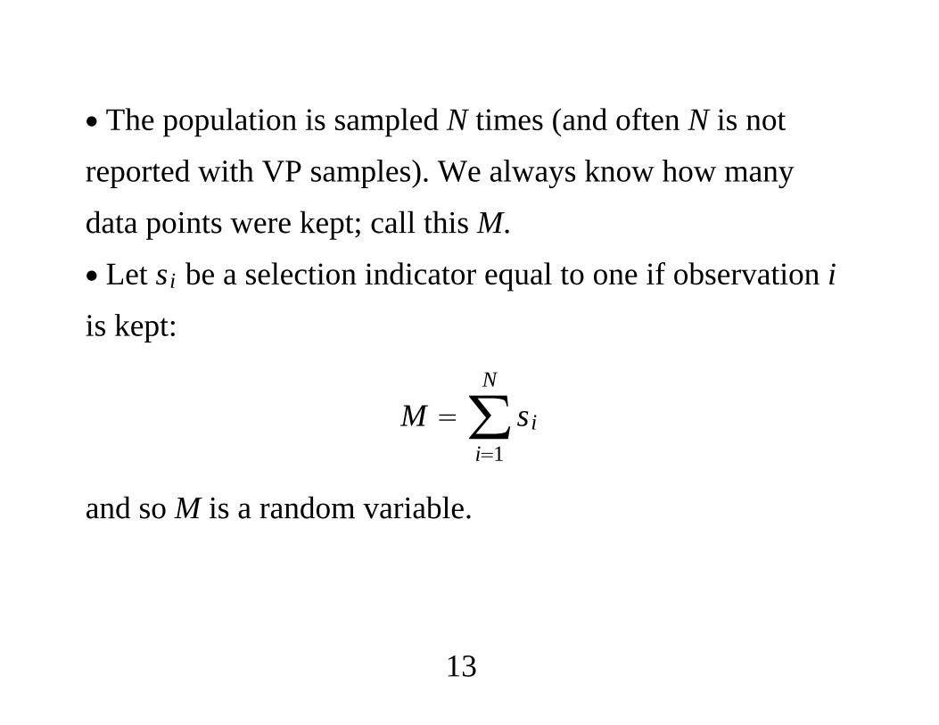
∙ The population is sampled N times (and often N is notreported with VP samples). We always know how manydata points were kept; call this M.∙ Let si be a selection indicator equal to one if observation iis kept:
M ∑i1
N
si
and so M is a random variable.
13
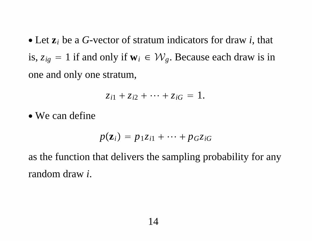
∙ Let zi be a G-vector of stratum indicators for draw i, thatis, zig 1 if and only if wi ∈ Wg. Because each draw is in
one and only one stratum,
zi1 zi2 ziG 1.
∙We can define
pzi p1zi1 pGziG
as the function that delivers the sampling probability for anyrandom draw i.
14
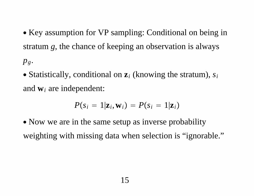
∙ Key assumption for VP sampling: Conditional on being instratum g, the chance of keeping an observation is alwayspg.
∙ Statistically, conditional on zi (knowing the stratum), si
and wi are independent:
Psi 1|zi,wi Psi 1|zi
∙ Now we are in the same setup as inverse probabilityweighting with missing data when selection is “ignorable.”
15
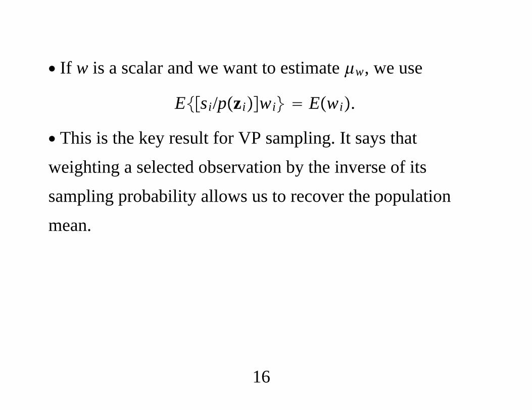
∙ If w is a scalar and we want to estimate w, we use
Esi/pziwi Ewi.
∙ This is the key result for VP sampling. It says thatweighting a selected observation by the inverse of itssampling probability allows us to recover the populationmean.
16

∙ It follows that
w N−1∑i1
N
si/pziwi
is a consistent estimator of Ewi.∙We can also write w as
M/NM−1∑i1
N
si/pziwi M−1∑i1
M
viwi
where vi M/N/pzi.
17

2. Regression Analysis∙ Almost any estimation method can be used with SS or VPsampled data, including OLS. Let w x,y.∙ Linear population model:
y x u
∙ Consider two exogeneity assumptions on x:
Eu|x 0
Ex′u 0
18
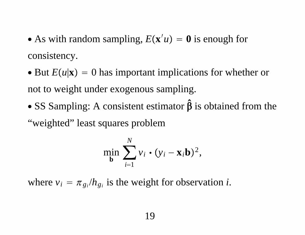
∙ As with random sampling, Ex′u 0 is enough forconsistency.∙ But Eu|x 0 has important implications for whether ornot to weight under exogenous sampling.
∙ SS Sampling: A consistent estimator is obtained from the
“weighted” least squares problem
minb∑i1
N
vi yi − xib2,
where vi gi /hgi is the weight for observation i.
19
∙ The weighted estimator is consistent for any stratificationscheme, whether stratification depends on x or y or both.∙ The weighting is not to address heteroskedasticity. Wereweight the sample in order to consistently estimate thepopulation parameter .
∙ In the population it may or may not be true that Varu|x isconstant.
∙ How can we conduct valid inference using ?
20

∙ Can show a proper asymptotic variance estimator is
∑i1
N
gi /hgixi′xi
−1
∑g1
G
g/hg2 ∑i1
Ng
xgi′ ûgi − xg
′ ûgxgi′ ûgi − xg
′ ûg′
∑i1
N
gi /hgixi′xi
−1
,
where xg′ ûg Ng
−1∑i1Ng xgi
′ ûgi.
21
∙ The usual White estimator ignores the information on thestrata of the observations: it drops the within-stratum
averages, xg′ ûg.
∙ The correct estimate is always smaller than the usualWhite estimate – an algebraic fact and legitimate based onasymptotic theory.
22
∙ Stata has a survey sampling option, svy, that will compute
the correct estimator provided stratum membership isincluded along with the weights.∙ If only the weights are provided, the larger asymptoticvariance is computed.∙ The command that describes the nature of the stratificationand weights is svyset.
23

∙ There is no gain from subtracting off within-strata meanswhen
Ex′u|w ∈ Wg 0, g 1, . . . ,G.
∙ Then Exg′ ug 0 and so
Ng−1∑
i1
Ng
xgi′ ûgi
p→ 0 as Ng → .
∙ A sufficient condition is Eu|x 0 and stratification isbased on x.
24
∙ The debate about whether or not to weight whenstratification depends on x centers on two facts:1. If Eu|x 0 and stratification is based on x, theunweighted estimator is also consistent. If we addVaru|x 2 then the weighted estmator is asymptoticallyless efficient than the unweighted (OLS) estimator. Thisargues against weighting.
25
2. The unweighted estimator is generally inconsistent for if
we only assume
y x u, Ex′u 0,
even when stratification is based on x. The weightedestimator consistently estimates under Ex′u 0. This
argues for weighting.
26
Summary∙ If stratification depends on y, or other variables correlatedwith u, we need to use the weights for consistent estimation.This is true even if Eu|x 0.∙When stratification depends on x we should still weight ifwe want to ensure that consistent estimation of thepopulation linear projection of y on x (where x may includenonlinear functions).
27

∙ If the linear projection is the same as the conditional mean,and we think homoskedasticity is reasonable, then we shouldnot weight (when stratification depends on x). This is anefficiency issue.∙ If Eu|x 0 and Varu|x ≠ Varu, we cannot generallyrank the weighted and unweighted estimators in terms ofefficiency.∙ Analogous results hold for maximum likelihood,quasi-MLE, nonlinear least squares, instrumental variables.
28
∙ Results for VP sampling are similar.1. With endogenous stratification one must use theprobability weights for consistency.2. With exogenous stratification the same results andconsiderations from the SS case hold.
29

∙ There are some additional results for VP sampling:1. The Huber-White sandwich matrix applied to theweighted objective function (with weights 1/pg) is consistent
when the known pg are used. Otherwise it is conservative.
2. Improve asymptotic efficiency by using the retentionfrequencies, pg Mg/Ng, assuming we observe Ng (number
of times stratum g was sampled).
30
Example: G 6 strata with variable probability sampling inaddition to an initial stratification.∙Within each stratum, VP sampling is used. The weightsaccount for SS and VP sampling.
31
. use http://www.stata-press.com/data/r10/nmihs
. des idnum stratan finwgt marital age race birthwgt
storage display valuevariable name type format label variable label----------------------------------------------------------------------------idnum long %10.0f ID numberstratan byte %8.0g Strata indicator 1-6finwgt double %10.0g Adjusted sampling weightmarital byte %8.0g marital 0single, 1marriedage byte %8.0g Mother’s age in yearsrace byte %8.0g race Race: 1black, 0white/otherbirthwgt int %8.0g Birthweight in grams
32
. svyset [pweight finwgt] , strata(stratan)
pweight: finwgtVCE: linearized
Single unit: missingStrata 1: stratan
SU 1: observationsFPC 1: zero
. mean birthwgt
Mean estimation Number of obs 9946
--------------------------------------------------------------| Mean Std. Err. [95% Conf. Interval]
-------------------------------------------------------------birthwgt | 2845.094 9.861422 2825.764 2864.424
--------------------------------------------------------------
33
. svy: mean birthwgt(running mean on estimation sample)
Survey: Mean estimation
Number of strata 6 Number of obs 9946Number of PSUs 9946 Population size 3895562
Design df 9940
--------------------------------------------------------------| Linearized| Mean Std. Err. [95% Conf. Interval]
-------------------------------------------------------------birthwgt | 3355.452 6.402741 3342.902 3368.003
--------------------------------------------------------------
34

. svyset [pweight finwgt]
pweight: finwgtVCE: linearized
Single unit: missingStrata 1: one
SU 1: observationsFPC 1: zero
. svy: mean birthwgt(running mean on estimation sample)
Survey: Mean estimation
Number of strata 1 Number of obs 9946Number of PSUs 9946 Population size 3895562
Design df 9945
--------------------------------------------------------------| Linearized| Mean Std. Err. [95% Conf. Interval]
-------------------------------------------------------------birthwgt | 3355.452 6.933529 3341.861 3369.044
--------------------------------------------------------------
. * So the standard error is, as expected, larger if we ignore the strata.
35
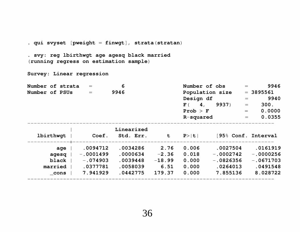
. qui svyset [pweight finwgt], strata(stratan)
. svy: reg lbirthwgt age agesq black married(running regress on estimation sample)
Survey: Linear regression
Number of strata 6 Number of obs 9946Number of PSUs 9946 Population size 3895561
Design df 9940F( 4, 9937) 300.Prob F 0.0000R-squared 0.0355
----------------------------------------------------------------------------| Linearized
lbirthwgt | Coef. Std. Err. t P|t| [95% Conf. Interval---------------------------------------------------------------------------
age | .0094712 .0034286 2.76 0.006 .0027504 .0161919agesq | -.0001499 .0000634 -2.36 0.018 -.0002742 -.0000256black | -.074903 .0039448 -18.99 0.000 -.0826356 -.0671703
married | .0377781 .0058039 6.51 0.000 .0264013 .0491548_cons | 7.941929 .0442775 179.37 0.000 7.855136 8.028722
----------------------------------------------------------------------------
36
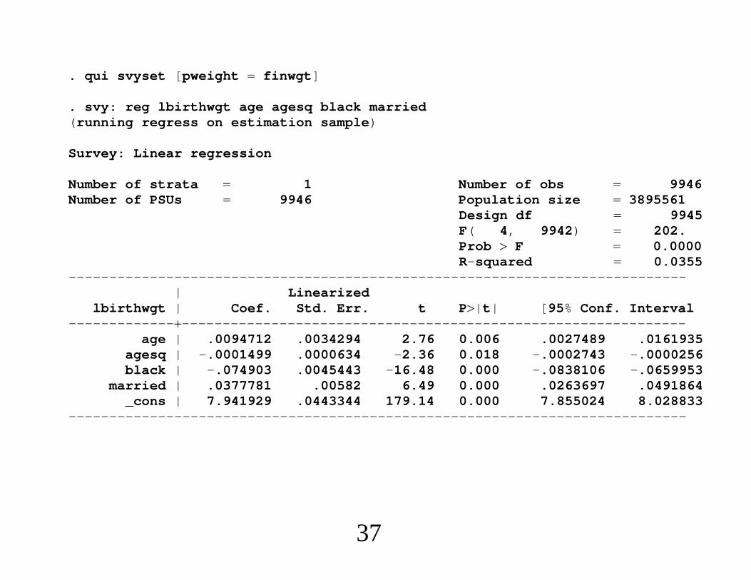
. qui svyset [pweight finwgt]
. svy: reg lbirthwgt age agesq black married(running regress on estimation sample)
Survey: Linear regression
Number of strata 1 Number of obs 9946Number of PSUs 9946 Population size 3895561
Design df 9945F( 4, 9942) 202.Prob F 0.0000R-squared 0.0355
----------------------------------------------------------------------------| Linearized
lbirthwgt | Coef. Std. Err. t P|t| [95% Conf. Interval---------------------------------------------------------------------------
age | .0094712 .0034294 2.76 0.006 .0027489 .0161935agesq | -.0001499 .0000634 -2.36 0.018 -.0002743 -.0000256black | -.074903 .0045443 -16.48 0.000 -.0838106 -.0659953
married | .0377781 .00582 6.49 0.000 .0263697 .0491864_cons | 7.941929 .0443344 179.14 0.000 7.855024 8.028833
----------------------------------------------------------------------------
37

. reg lbirthwgt age agesq black married, robust
Linear regression Number of obs 9946F( 4, 9941) 28.Prob F 0.0000R-squared 0.0114Root MSE .49611
----------------------------------------------------------------------------| Robust
lbirthwgt | Coef. Std. Err. t P|t| [95% Conf. Interval---------------------------------------------------------------------------
age | .0161755 .0074639 2.17 0.030 .0015448 .0308062agesq | -.0003198 .000138 -2.32 0.020 -.0005902 -.0000493black | -.0136733 .0116097 -1.18 0.239 -.0364307 .0090841
married | .0961381 .0129681 7.41 0.000 .0707181 .1215582_cons | 7.615568 .0969574 78.55 0.000 7.425512 7.805624
----------------------------------------------------------------------------
38
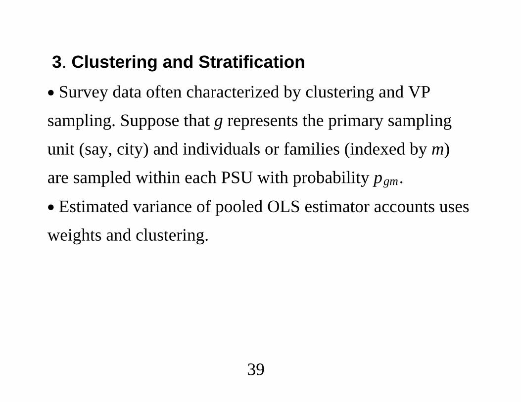
3. Clustering and Stratification∙ Survey data often characterized by clustering and VPsampling. Suppose that g represents the primary samplingunit (say, city) and individuals or families (indexed by m)are sampled within each PSU with probability pgm.
∙ Estimated variance of pooled OLS estimator accounts usesweights and clustering.
39
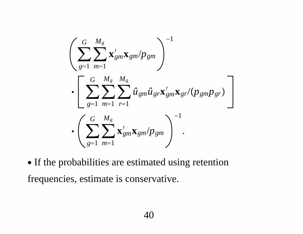
∑g1
G
∑m1
Mg
xgm′ xgm/pgm
−1
∑g1
G
∑m1
Mg
∑r1
Mg
ûgmûgrxgm′ xgr/pgmpgr
∑g1
G
∑m1
Mg
xgm′ xgm/pgm
−1
.
∙ If the probabilities are estimated using retentionfrequencies, estimate is conservative.
40

∙Multi-stage sampling schemes introduce even morecomplications.∙ Let there be S strata (e.g., states in the U.S.), exhaustiveand mutually exclusive.∙Within stratum s, there are Cs clusters (e.g.,neighborhoods).∙ Large-sample approximations: the number of clusterssampled, Ns, gets large. This allows for arbitrary correlation(say, across households) within cluster.
41
∙Within stratum s and cluster c, let there be Msc total units(household or individuals).∙ The total number of units in the population is
M ∑s1
S
∑c1
Cs
Msc.
42
∙ List all population values of a variable z:
zscmo : m 1, . . . ,Msc,c 1, . . . ,Cs, s 1, . . . ,S,
so the population mean is
M−1∑s1
S
∑c1
Cs
∑m1
Msc
zscmo .
Define the total in the population as
∑s1
S
∑c1
Cs
∑m1
Msc
zscmo M.
43
∙ Totals within each cluster and then stratum are,respectively,
sc ∑m1
Msc
zscmo
s ∑c1
Cs
sc
44
∙ Sampling scheme:1. For each stratum s, randomly draw Ns clusters, withreplacement. (The “with replacement” assumption is notrealistic but is a fine approximation for “large” Cs.)2. For each cluster c drawn in step 1, randomly sample Ksc
households (with replacement).
45
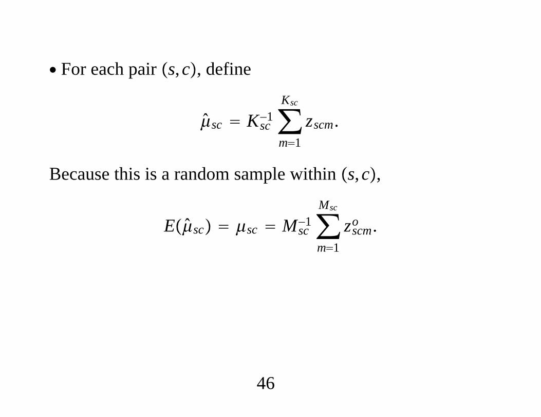
∙ For each pair s,c, define
sc Ksc−1∑
m1
Ksc
zscm.
Because this is a random sample within s,c,
Esc sc Msc−1∑
m1
Msc
zscmo .
46
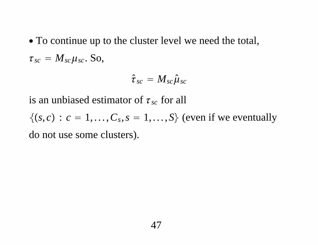
∙ To continue up to the cluster level we need the total,sc Mscsc. So,
sc Mscsc
is an unbiased estimator of sc for alls,c : c 1, . . . ,Cs, s 1, . . . ,S (even if we eventuallydo not use some clusters).
47
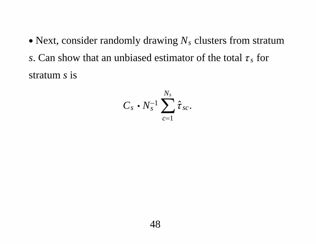
∙ Next, consider randomly drawing Ns clusters from stratums. Can show that an unbiased estimator of the total s forstratum s is
Cs Ns−1∑
c1
Ns
sc.
48

∙ Finally, the total in the population is estimated as
∑s1
S
Cs Ns−1∑
c1
Ns
sc ≡ ∑s1
S
∑c1
Ns
∑m1
Ksc
sczscm
where, after simple algebra, the weight for stratum-clusterpair s,c is
sc ≡ CsNs
MscKsc
.
49

∙ Note how
sc ≡ CsNs
MscKsc
accounts for under- or over-sampled clusters within strataand under- or over-sampled units within clusters.∙ These weights appear in the literature on complex surveysampling, sometimes without Msc/Ksc when each cluster issampled as a complete unit, and so Msc/Ksc 1.
50
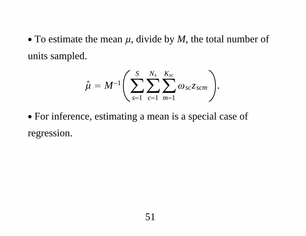
∙ To estimate the mean , divide by M, the total number of
units sampled.
M−1 ∑s1
S
∑c1
Ns
∑m1
Ksc
sczscm .
∙ For inference, estimating a mean is a special case ofregression.
51
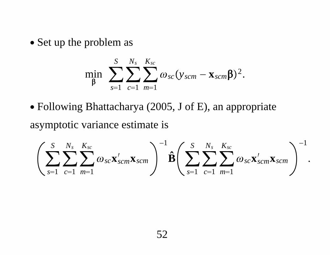
∙ Set up the problem as
min∑s1
S
∑c1
Ns
∑m1
Ksc
scyscm − xscm2.
∙ Following Bhattacharya (2005, J of E), an appropriateasymptotic variance estimate is
∑s1
S
∑c1
Ns
∑m1
Ksc
scxscm′ xscm
−1
B ∑s1
S
∑c1
Ns
∑m1
Ksc
scxscm′ xscm
−1
.
52
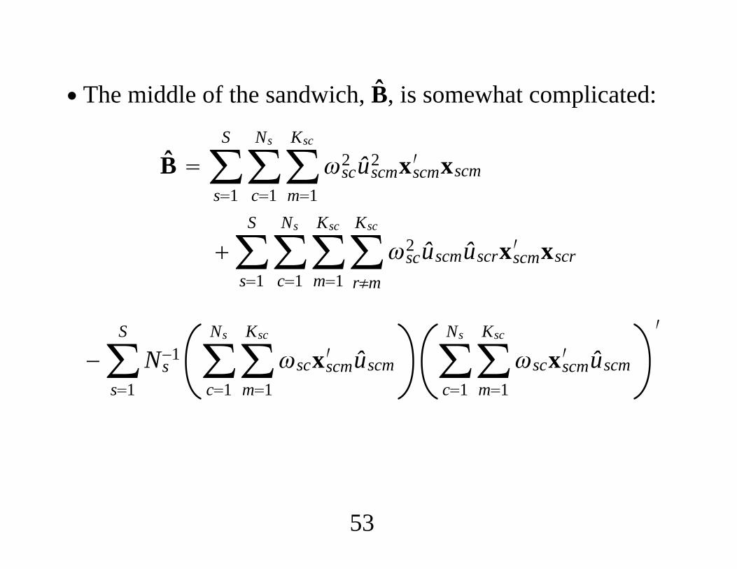
∙ The middle of the sandwich, B, is somewhat complicated:
B ∑s1
S
∑c1
Ns
∑m1
Ksc
sc2 ûscm
2 xscm′ xscm
∑s1
S
∑c1
Ns
∑m1
Ksc
∑r≠m
Ksc
sc2 ûscmûscrxscm
′ xscr
−∑s1
S
Ns−1 ∑
c1
Ns
∑m1
Ksc
scxscm′ ûscm ∑
c1
Ns
∑m1
Ksc
scxscm′ ûscm
′
53
∙ The first part of B is obtained using the White“heteroskedasticity”-robust form.∙ The second piece accounts for the cluster sampling.∙ The third piece reduces the variance by accounting for thenonzero means of the “score” within strata.∙With linearization via the delta method, similar formulashold for nonlinear models.
54
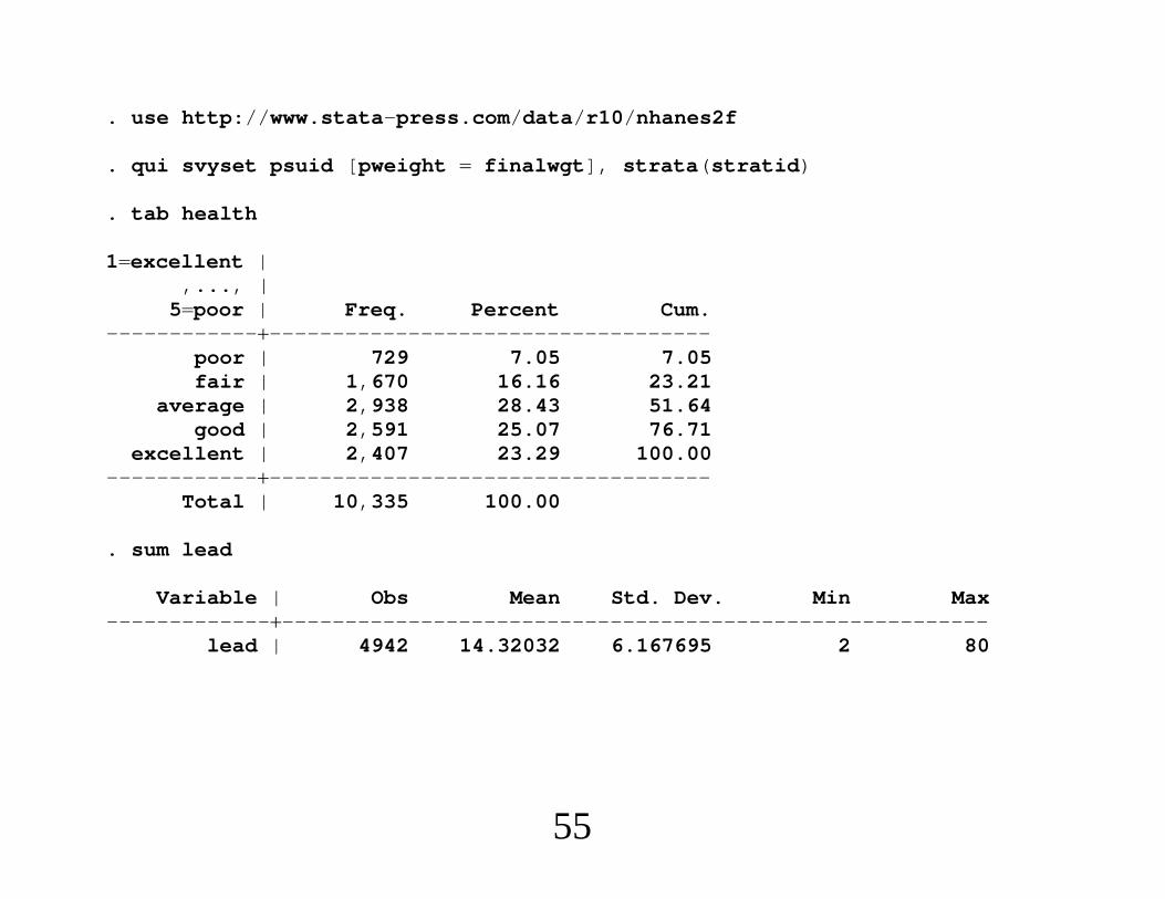
. use http://www.stata-press.com/data/r10/nhanes2f
. qui svyset psuid [pweight finalwgt], strata(stratid)
. tab health
1excellent |,..., |
5poor | Freq. Percent Cum.-----------------------------------------------
poor | 729 7.05 7.05fair | 1,670 16.16 23.21
average | 2,938 28.43 51.64good | 2,591 25.07 76.71
excellent | 2,407 23.29 100.00-----------------------------------------------
Total | 10,335 100.00
. sum lead
Variable | Obs Mean Std. Dev. Min Max---------------------------------------------------------------------
lead | 4942 14.32032 6.167695 2 80
55
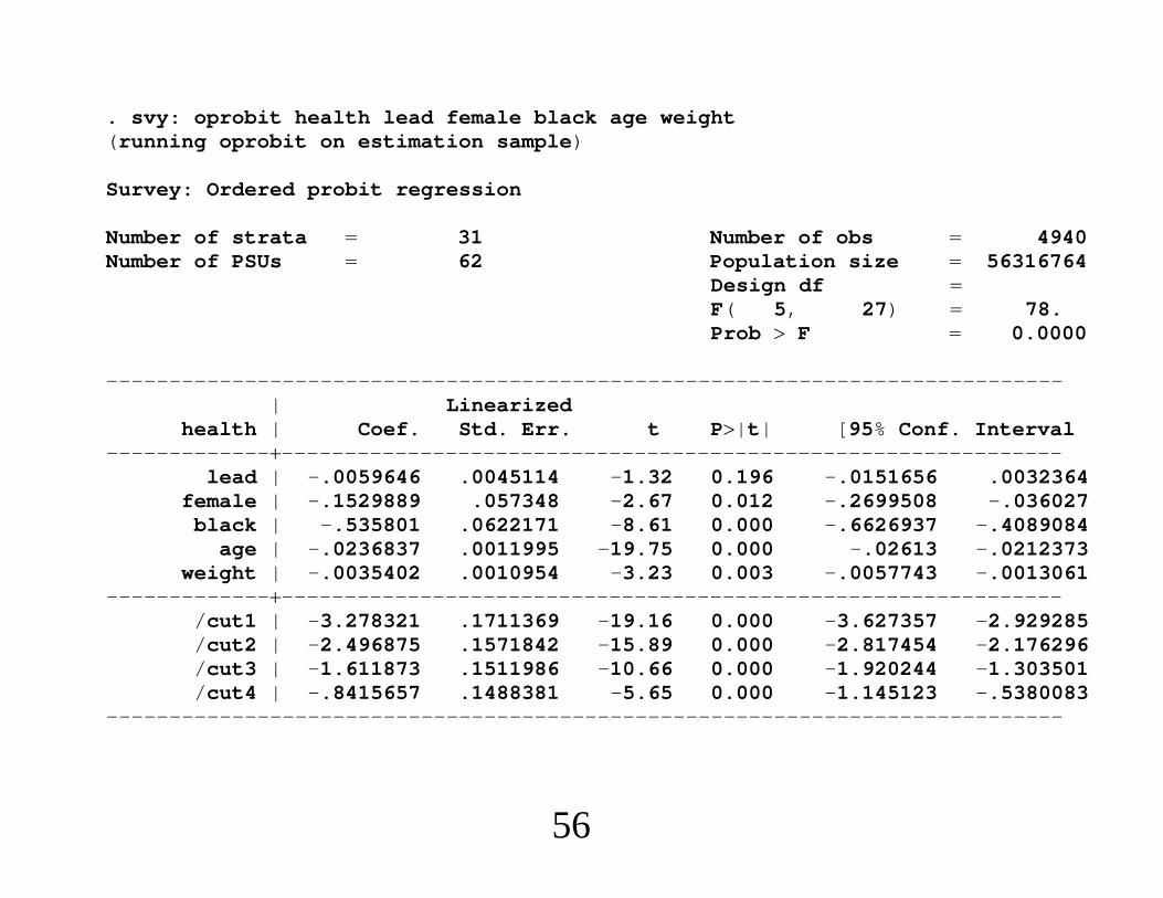
. svy: oprobit health lead female black age weight(running oprobit on estimation sample)
Survey: Ordered probit regression
Number of strata 31 Number of obs 4940Number of PSUs 62 Population size 56316764
Design df F( 5, 27) 78.Prob F 0.0000
----------------------------------------------------------------------------| Linearized
health | Coef. Std. Err. t P|t| [95% Conf. Interval---------------------------------------------------------------------------
lead | -.0059646 .0045114 -1.32 0.196 -.0151656 .0032364female | -.1529889 .057348 -2.67 0.012 -.2699508 -.036027
black | -.535801 .0622171 -8.61 0.000 -.6626937 -.4089084age | -.0236837 .0011995 -19.75 0.000 -.02613 -.0212373
weight | -.0035402 .0010954 -3.23 0.003 -.0057743 -.0013061---------------------------------------------------------------------------
/cut1 | -3.278321 .1711369 -19.16 0.000 -3.627357 -2.929285/cut2 | -2.496875 .1571842 -15.89 0.000 -2.817454 -2.176296/cut3 | -1.611873 .1511986 -10.66 0.000 -1.920244 -1.303501/cut4 | -.8415657 .1488381 -5.65 0.000 -1.145123 -.5380083
----------------------------------------------------------------------------
56
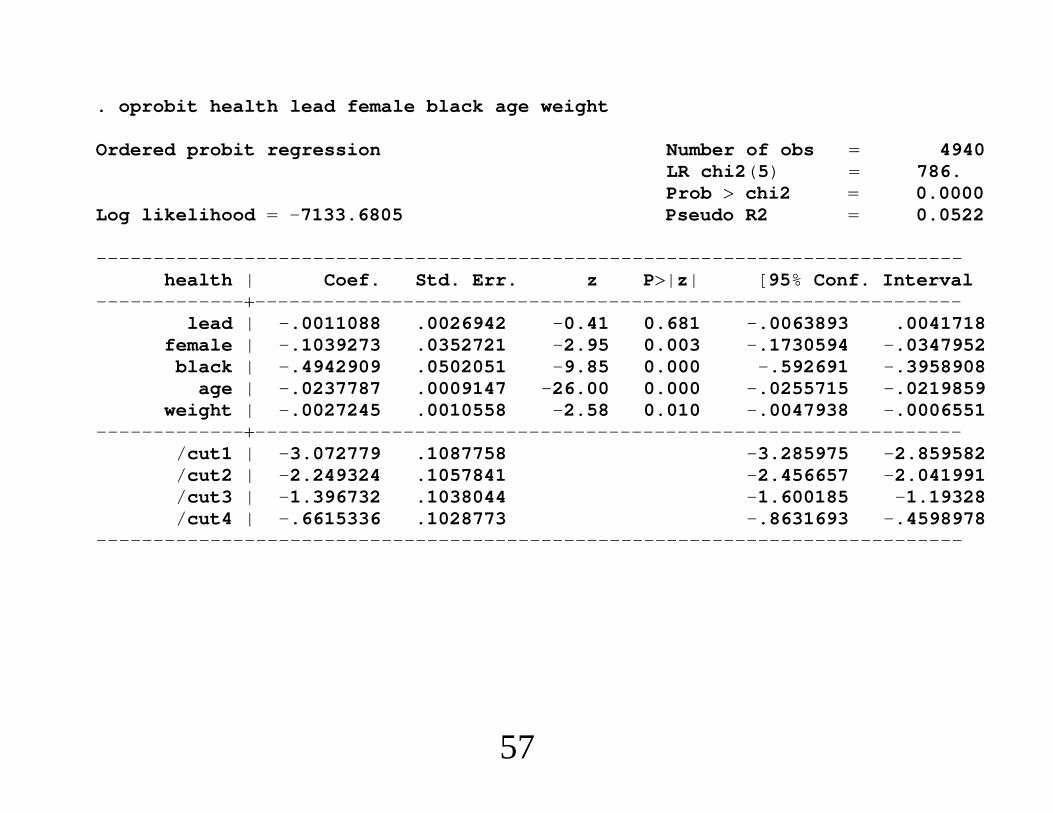
. oprobit health lead female black age weight
Ordered probit regression Number of obs 4940LR chi2(5) 786.Prob chi2 0.0000
Log likelihood -7133.6805 Pseudo R2 0.0522
----------------------------------------------------------------------------health | Coef. Std. Err. z P|z| [95% Conf. Interval
---------------------------------------------------------------------------lead | -.0011088 .0026942 -0.41 0.681 -.0063893 .0041718
female | -.1039273 .0352721 -2.95 0.003 -.1730594 -.0347952black | -.4942909 .0502051 -9.85 0.000 -.592691 -.3958908
age | -.0237787 .0009147 -26.00 0.000 -.0255715 -.0219859weight | -.0027245 .0010558 -2.58 0.010 -.0047938 -.0006551
---------------------------------------------------------------------------/cut1 | -3.072779 .1087758 -3.285975 -2.859582/cut2 | -2.249324 .1057841 -2.456657 -2.041991/cut3 | -1.396732 .1038044 -1.600185 -1.19328/cut4 | -.6615336 .1028773 -.8631693 -.4598978
----------------------------------------------------------------------------
57

"Econometrics of Cross Section and Panel Data"
Lecture 10
Partial Identification
Guido Imbens
Cemmap Lectures, UCL, June 2014

1. Introduction
2. Example I: Missing Data
3. Example II: Returns to Schooling
4. Example III: Initial Conditions Problems in Panel Data
5. Example IV: Auction Data
6. Example V: Entry Models
7. Estimation and Inference
1

1. Introduction
Traditionally in constructing statistical or econometric models
researchers look for models that are (point-)identified: given
a large (infinite) data set, one can infer without uncertainty
what the values are of the objects of interest.
It would appear that a model where we cannot learn the pa-
rameter values even in infinitely large samples would not be
very useful.
However, it turns out that even in cases where we cannot learn
the value of the estimand exactly in large samples, in many
cases we can still learn a fair amount, even in finite samples. A
research agenda initiated by Manski has taken this perspective.
2
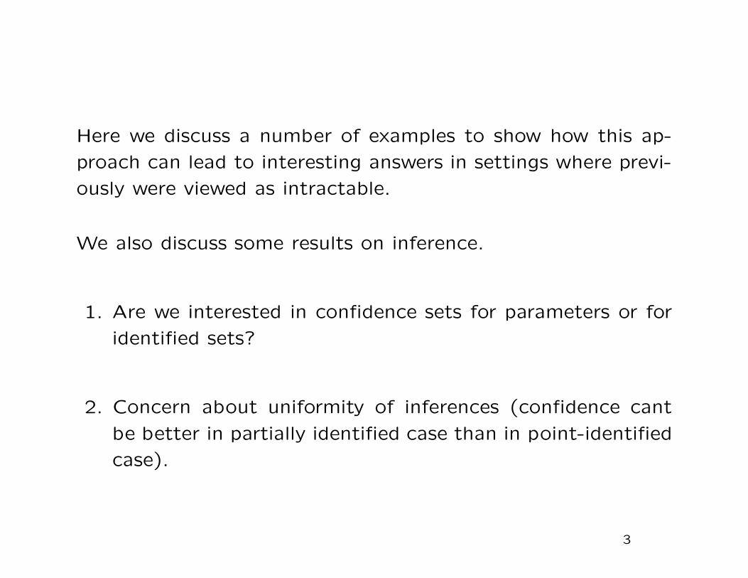
Here we discuss a number of examples to show how this ap-
proach can lead to interesting answers in settings where previ-
ously were viewed as intractable.
We also discuss some results on inference.
1. Are we interested in confidence sets for parameters or for
identified sets?
2. Concern about uniformity of inferences (confidence cant
be better in partially identified case than in point-identified
case).
3
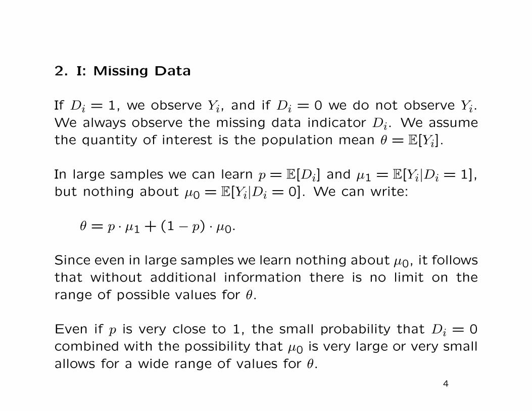
2. I: Missing Data
If Di = 1, we observe Yi, and if Di = 0 we do not observe Yi.
We always observe the missing data indicator Di. We assume
the quantity of interest is the population mean θ = E[Yi].
In large samples we can learn p = E[Di] and µ1 = E[Yi|Di = 1],
but nothing about µ0 = E[Yi|Di = 0]. We can write:
θ = p · µ1 + (1 − p) · µ0.
Since even in large samples we learn nothing about µ0, it follows
that without additional information there is no limit on the
range of possible values for θ.
Even if p is very close to 1, the small probability that Di = 0
combined with the possibility that µ0 is very large or very small
allows for a wide range of values for θ.
4
Now suppose we know that the variable of interest is binary:
Yi ∈ 0,1. Then natural (not data-informed) lower and upper
bounds for µ0 are 0 and 1 respectively. This implies bounds on
θ:
θ ∈ [θLB, θUB] = [p · µ1, p · µ1 + (1 − p)] .
These bounds are sharp, in the sense that without additional
information we can not improve on them.
Formally, for all values θ in [θLB, θUB], we can find a joint distri-
bution of (Yi,Wi) that is consistent with the joint distribution
of the observed data and with θ.
5
We can also obtain informative bounds if we modify the object
of interest a little bit.
Suppose we are interested in the median of Yi, θ0.5 = med(Yi).
Define qτ(Yi) to be the τ quantile of the conditional distribution
of Yi given Di = 1. Then the median cannot be larger than
q1/(2p)(Yi) because even if all the missing values were large, we
know that at least p · (1/(2p)) = 1/2 of the units have a value
less than or equal to q1/(2p)(Yi).
Then, if p > 1/2, we can infer that the median must satisfy
θ0.5 ∈ [θLB, θUB] =[
q(2p−1)/(2p)(Yi), q1/(2p)(Yi)]
,
and we end up with a well defined, and, depending on the data,
more or less informative identified interval for the median.
6
If fewer than 50% of the values are observed, or p < 1/2,
then we cannot learn anything about the median of Yi without
additional information (for example, a bound on the values of
Yi), and the interval is (−∞,∞).
More generally, we can obtain bounds on the τ quantile of the
distribution of Yi, equal to
θτ ∈ [θLB, θUB] =[
q(τ−(1−p))/p(Yi|Di = 1), qτ/p(Yi|Di = 1)]
.
which is bounded if the probability of Yi being missing is less
than min(τ,1 − τ).
7
3. Example II: Returns to Schooling
Manski-Pepper are interested in estimating returns to school-
ing. They start with an individual level response function Yi(w).
∆(s, t) = E[Yi(t)− Yi(s)],
is the object of interest, the difference in average log earnings
given t rather than s years of schooling.
Wi is the actual years of school, and Yi = Yi(Wi) be the actual
log earnings.
If one makes an unconfoundedness/exogeneity assumption that
Yi(w) ⊥⊥ Wi | Xi,
for some set of covariates, one can estimate ∆(s, t) consistently
given some support conditions. MP relax this assumption.
8
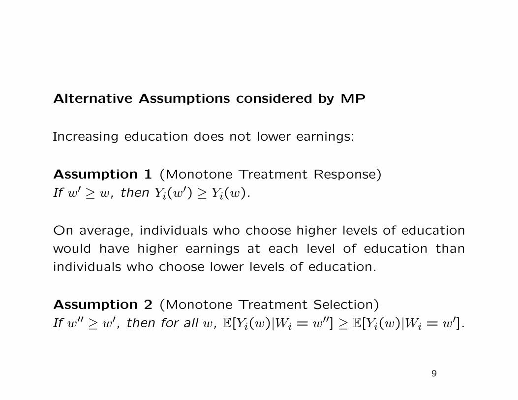
Alternative Assumptions considered by MP
Increasing education does not lower earnings:
Assumption 1 (Monotone Treatment Response)
If w′ ≥ w, then Yi(w′) ≥ Yi(w).
On average, individuals who choose higher levels of education
would have higher earnings at each level of education than
individuals who choose lower levels of education.
Assumption 2 (Monotone Treatment Selection)
If w′′ ≥ w′, then for all w, E[Yi(w)|Wi = w′′] ≥ E[Yi(w)|Wi = w′].
9
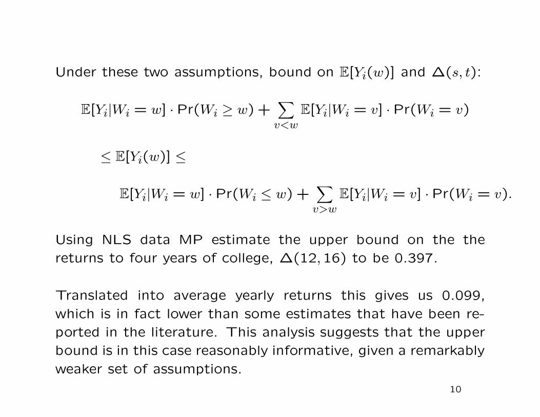
Under these two assumptions, bound on E[Yi(w)] and ∆(s, t):
E[Yi|Wi = w] · Pr(Wi ≥ w) +∑
v<w
E[Yi|Wi = v] · Pr(Wi = v)
≤ E[Yi(w)] ≤
E[Yi|Wi = w] · Pr(Wi ≤ w) +∑
v>w
E[Yi|Wi = v] ·Pr(Wi = v).
Using NLS data MP estimate the upper bound on the the
returns to four years of college, ∆(12,16) to be 0.397.
Translated into average yearly returns this gives us 0.099,
which is in fact lower than some estimates that have been re-
ported in the literature. This analysis suggests that the upper
bound is in this case reasonably informative, given a remarkably
weaker set of assumptions.
10
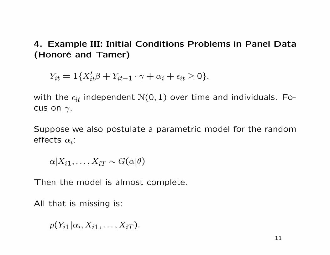
4. Example III: Initial Conditions Problems in Panel Data
(Honore and Tamer)
Yit = 1X′itβ + Yit−1 · γ + αi + εit ≥ 0,
with the εit independent N(0,1) over time and individuals. Fo-
cus on γ.
Suppose we also postulate a parametric model for the random
effects αi:
α|Xi1, . . . , XiT ∼ G(α|θ)
Then the model is almost complete.
All that is missing is:
p(Yi1|αi, Xi1, . . . , XiT ).
11

HT assume a discrete distribution for α, with a finite and
known set of support points. They fix the support to be
−3,−2.8, . . . ,2.8,3, with unknown probabilities.
In the case with T = 3 they find that the range of values for
γ consistent with the data generating process (the identified
set) is very narrow.
If γ is in fact equal to zero, the width of the set is zero.
If the true value is γ = 1, then the width of the interval is
approximately 0.1. (It is largest for γ close to, but not equal
to, -1.) See Figure 1, taken from HT.
The HT analysis shows nicely the power of the partial identifi-
cation approach: A problem that had been viewed as essentially
intractable, with many non-identification results, was shown to
admit potentially precise inferences. Point identification is not
a big issue here.
12


5. Example IV: Auction Data
Haile and Tamer study English or oral ascending bid auctions.
In such auctions bidders offer increasingly higher prices until
only one bidder remains. HT focus on a symmetric independent
private values model. In auction t, bidder i has a value νit,
drawn independently from the value for bidder j, with cdf Fν(v)
HT are interested in the value distribution Fν(v). This is as-
sumed to be the same in each auction (after adjusting for
observable auction characteristics).
One can imagine observing exactly when each bidder leaves the
auction, thus directly observing their valuations. This is not
what is typically observed. For each bidder we do not know
at any point in time whether they are still participating unless
they subsequently make a higher bid.
13

Haile-Tamer Assumptions
Assumption 3 No bidder ever bids more than their valuation
Assumption 4 No bidder will walk away and let another bidder
win the auction if the winning bid is lower than their own
valuation
14
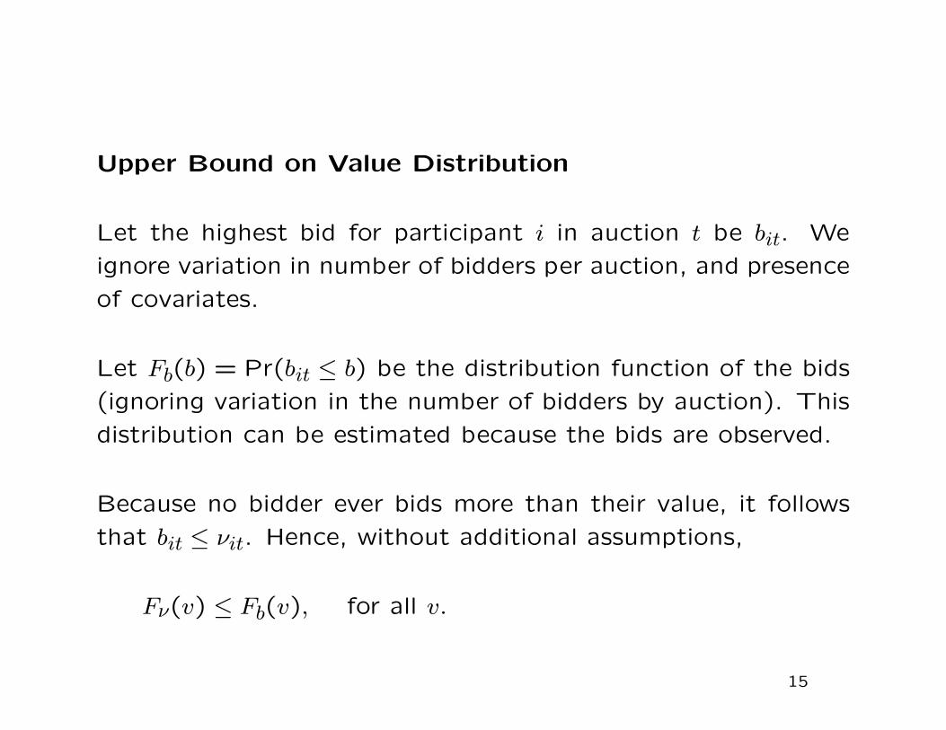
Upper Bound on Value Distribution
Let the highest bid for participant i in auction t be bit. We
ignore variation in number of bidders per auction, and presence
of covariates.
Let Fb(b) = Pr(bit ≤ b) be the distribution function of the bids
(ignoring variation in the number of bidders by auction). This
distribution can be estimated because the bids are observed.
Because no bidder ever bids more than their value, it follows
that bit ≤ νit. Hence, without additional assumptions,
Fν(v) ≤ Fb(v), for all v.
15
Lower Bound on Value Distribution
The second highest of the values among the n participants
in auction t must be less than or equal to the winning bid.
This follows from the assumption that no participant will let
someone else win with a bid below their valuation.
Let Fν,m:n(v) denote the mth order statistic in a random sample
of size n from the value distribution, and let FB,n:n(b) denote
the distribution of the winning bid in auctions with n partici-
pants. Then
FB,n:n(v) ≤ Fν,n−1:n(v).
The distribution of the any order statistic is monotonically re-
lated to the distribution of the parent distribution, and so a
lower bound on Fν,n−1:n(v) implies a lower bound on Fν(v).
16

6. Example V: Entry Models (Cilberto & Tamer)
Suppose two firms, A and B, contest a set of markets. In
market m, m = 1, . . . ,M , the profits for firms A and B are
πAm = αA + δA · dBm + εAm, πBm = αB + δB · dAm + εBm.
where dFm = 1 if firm F is present in market m, for F ∈ A,B,and zero otherwise.
Decisions assuming complete information satisfy Nash equilib-
rium condition
dAm = 1πAm ≥ 0, dBm = 1πBm ≥ 0.
17
Incomplete Model
For pairs of values (εAm, εBm) such that
−αA < εA ≤ −αA − δA, −αB < εB ≤ −αB − δB,
both (dA, dB) = (0,1) and (dA, dB) = (1,0) satisfy the profit
maximization condition.
In the terminology of this literature, the model is incomplete.
It does not specify the outcomes given the inputs. Missing is
an equilibrium selection mechanism, which is typically difficult
to justify.
Figure 1, adapted from CM, shows the different regions in the
(εAm, εBm) space.
18
Implication: Inequality Conditions
The implication of this is that the probability of the outcome
(dAm, dBm) = (0,1) cannot be written as a function of the
parameters of the model, θ = (αA, δA, αB, δB), even given dis-
tributional assumptions on (εAm, εBm).
Instead the model implies a lower and upper bound on this
probability:
HL,01(θ) ≤ Pr ((dAm, dBm) = (0,1)) ≤ HU,01(θ).
Thus in general we can write the information about the pa-
rameters in large samples as
HL,00(θ)HL,01(θ)HL,10(θ)HL,11(θ)
≤
Pr ((dAm, dBm) = (0,0))Pr ((dAm, dBm) = (0,1))Pr ((dAm, dBm) = (1,0))Pr ((dAm, dBm) = (1,1))
≤
HU,00(θ)HU,01(θ)HU,11(θ)HU,11(θ)
.
19

7.A Estimation
Chernozhukov, Hong, and Tamer study Generalized Inequality
Restriction (GIR) setting:
E[ψ(Z, θ)] ≥ 0,
where ψ(z, θ) is known. Fits CT entry example
Define for a vector x the vector (x)+ to be the component-
wise non-negative part, and (x)− to be the component-wise
non-positive part, so that for all x, x = (x)− + (x)+.
20
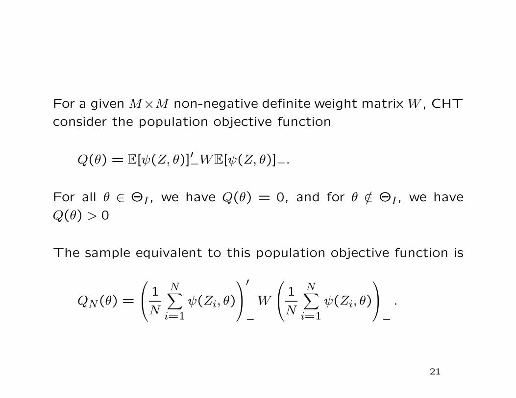
For a given M×M non-negative definite weight matrix W , CHT
consider the population objective function
Q(θ) = E[ψ(Z, θ)]′−WE[ψ(Z, θ)]−.
For all θ ∈ ΘI, we have Q(θ) = 0, and for θ /∈ ΘI, we have
Q(θ) > 0
The sample equivalent to this population objective function is
QN(θ) =
1
N
N∑
i=1
ψ(Zi, θ)
′
−W
1
N
N∑
i=1
ψ(Zi, θ)
−.
21
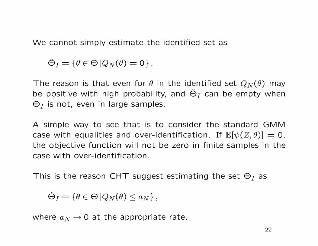
We cannot simply estimate the identified set as
ΘI = θ ∈ Θ |QN(θ) = 0 ,
The reason is that even for θ in the identified set QN(θ) may
be positive with high probability, and ΘI can be empty when
ΘI is not, even in large samples.
A simple way to see that is to consider the standard GMM
case with equalities and over-identification. If E[ψ(Z, θ)] = 0,
the objective function will not be zero in finite samples in the
case with over-identification.
This is the reason CHT suggest estimating the set ΘI as
ΘI = θ ∈ Θ |QN(θ) ≤ aN ,
where aN → 0 at the appropriate rate.
22
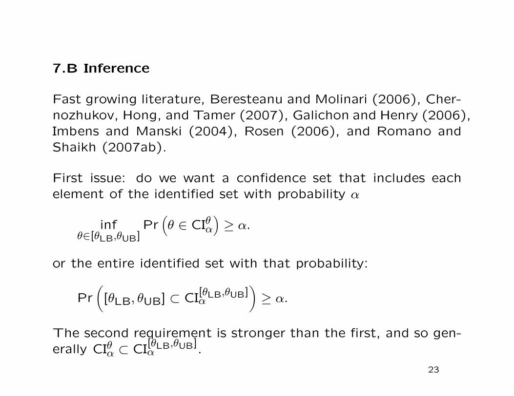
7.B Inference
Fast growing literature, Beresteanu and Molinari (2006), Cher-
nozhukov, Hong, and Tamer (2007), Galichon and Henry (2006),
Imbens and Manski (2004), Rosen (2006), and Romano and
Shaikh (2007ab).
First issue: do we want a confidence set that includes each
element of the identified set with probability α
infθ∈[θLB,θUB]
Pr(
θ ∈ CIθα
)
≥ α.
or the entire identified set with that probability:
Pr
(
[θLB, θUB] ⊂ CI[θLB,θUB]α
)
≥ α.
The second requirement is stronger than the first, and so gen-
erally CIθα ⊂ CI[θLB,θUB]α .
23
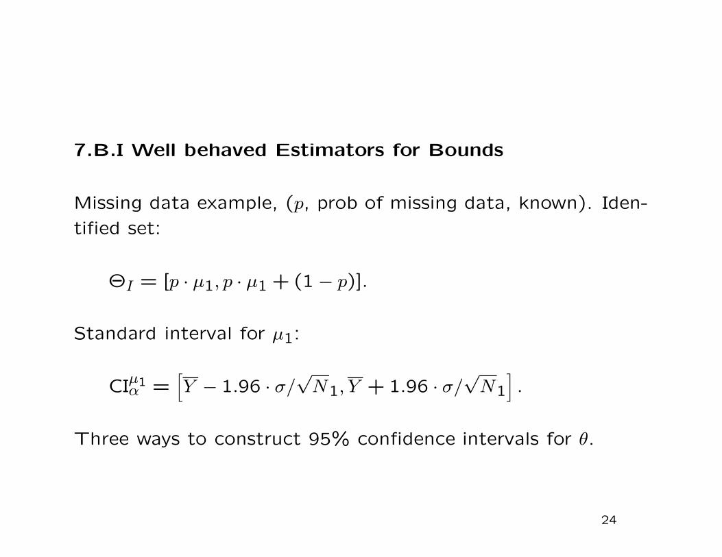
7.B.I Well behaved Estimators for Bounds
Missing data example, (p, prob of missing data, known). Iden-
tified set:
ΘI = [p · µ1, p · µ1 + (1 − p)].
Standard interval for µ1:
CIµ1α =
[
Y − 1.96 · σ/√N1, Y + 1.96 · σ/
√N1
]
.
Three ways to construct 95% confidence intervals for θ.
24
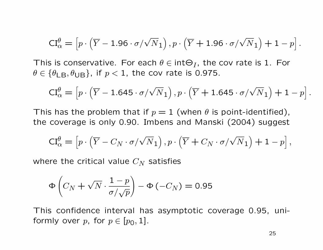
CIθα =[
p ·(
Y − 1.96 · σ/√N1
)
, p ·(
Y + 1.96 · σ/√N1
)
+ 1 − p]
.
This is conservative. For each θ ∈ intΘI, the cov rate is 1. For
θ ∈ θLB, θUB, if p < 1, the cov rate is 0.975.
CIθα =[
p ·(
Y − 1.645 · σ/√N1
)
, p ·(
Y + 1.645 · σ/√N1
)
+ 1 − p]
.
This has the problem that if p = 1 (when θ is point-identified),
the coverage is only 0.90. Imbens and Manski (2004) suggest
CIθα =[
p ·(
Y − CN · σ/√N1
)
, p ·(
Y + CN · σ/√N1
)
+ 1 − p]
,
where the critical value CN satisfies
Φ
(
CN +√N · 1 − p
σ/√p
)
− Φ(−CN) = 0.95
This confidence interval has asymptotic coverage 0.95, uni-
formly over p, for p ∈ [p0,1].
25

7.B.II Irregular Estimators for Bounds
Simple example of Generalized Inequality Restrictions (GIR)
set up.
E[X] ≥ θ, and E[Y ] ≥ θ.
The parameter space is Θ = [0,∞). Let µX = E[X], and
µY = E[Y ]. We have a random sample of size N of the pairs
(X,Y ). The identified set is
ΘI = [0,min(µX, µY )].
26
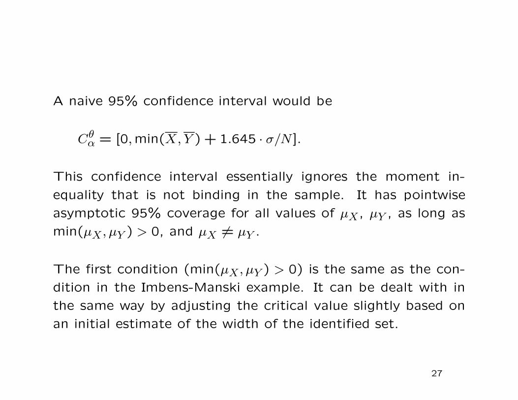
A naive 95% confidence interval would be
Cθα = [0,min(X,Y ) + 1.645 · σ/N ].
This confidence interval essentially ignores the moment in-
equality that is not binding in the sample. It has pointwise
asymptotic 95% coverage for all values of µX, µY , as long as
min(µX , µY ) > 0, and µX 6= µY .
The first condition (min(µX , µY ) > 0) is the same as the con-
dition in the Imbens-Manski example. It can be dealt with in
the same way by adjusting the critical value slightly based on
an initial estimate of the width of the identified set.
27
The naive confidence interval essentially assumes that the re-
searcher knows which moment conditions are binding. This is
true in large samples, unless there is a tie.
However, in finite samples ignoring uncertainty regarding the
set of binding moment inequalities may lead to a poor approxi-
mation, especially if there are many inequalities. One possibility
is to construct conservative confidence intervals (e.g., Pakes,
Porter, Ho, and Ishii, 2007). However, such intervals can be
unnecessarily conservative if there are moment inequalities that
are far from binding.
One would like construct confidence intervals that asymptot-
ically ignore irrelevant inequalities, and at the same time are
valid uniformly over the parameter space. For some propos-
als see Romano and Shaikh (2007a) and Andrews and Soares
(2007). Little is known about finite sample properties in real-
istic settings.
28

Econometrics of Cross Section and Panel DataLecture 11: Difference-in-Differences
Jeff WooldridgeMichigan State University
cemmap/PEPA, June 2014
1. The Basic Methodology2. How Should We View Uncertainty in DD Settings?3. The Donald and Lang Approach4. Multiple Groups and Time Periods5. Individual-Level Panel Data6. Semiparametric and Nonparametric Approaches
1
1. The Basic Methodology∙ Outcomes are observed for two groups for two timeperiods.∙ The treated group is subject to an intervention in thesecond period but not in the first period. The control groupis not exposed to the intervention during either period.∙ Structure can apply to repeated cross sections or paneldata. First assume repeated cross sections.
2
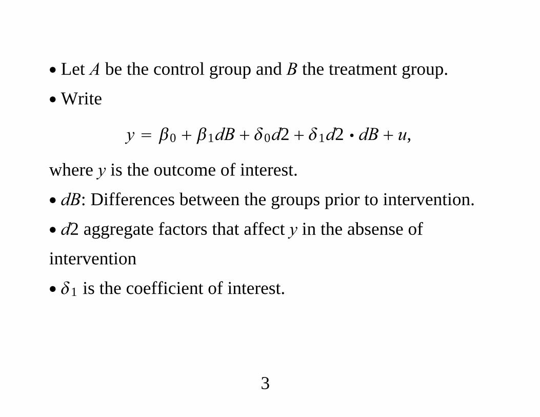
∙ Let A be the control group and B the treatment group.∙Write
y 0 1dB 0d2 1d2 dB u,
where y is the outcome of interest.∙ dB: Differences between the groups prior to intervention.∙ d2 aggregate factors that affect y in the absense ofintervention∙ 1 is the coefficient of interest.
3
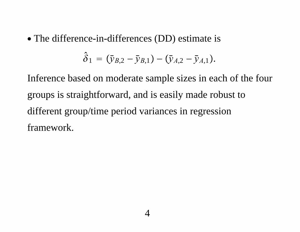
∙ The difference-in-differences (DD) estimate is
1 yB,2 − yB,1 − yA,2 − yA,1.
Inference based on moderate sample sizes in each of the fourgroups is straightforward, and is easily made robust todifferent group/time period variances in regressionframework.
4

∙ Can refine the definition of treatment and control groups.∙ Change in state health care policy aimed at elderly. Coulduse data only on people in the state with the policy change,both before and after the change, with the control groupbeing people 55 to 65 (say) and and the treatment groupbeing people over 65.∙ A standard DD analysis assumes that the paths of healthoutcomes for the younger and older groups would not besystematically different in the absense of intervention.
5

∙ Instead, use the same two groups from an “untreated” stateas an additional control.∙ dE is an indicator equal to one for someone over 65; dB isliving in the treated state; d2 is the second time period
y 0 1dB 2dE 3dB dE 0d2 1d2 dB 2d2 dE 3d2 dB dE u
where 3 is the average treatment effect.
6
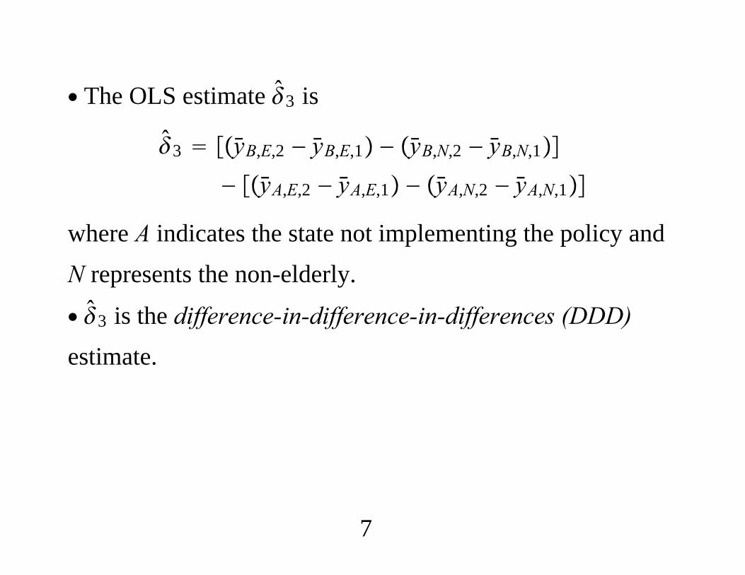
∙ The OLS estimate 3 is
3 yB,E,2 − yB,E,1 − yB,N,2 − yB,N,1
− yA,E,2 − yA,E,1 − yA,N,2 − yA,N,1
where A indicates the state not implementing the policy andN represents the non-elderly.
∙ 3 is the difference-in-difference-in-differences (DDD)estimate.
7
∙ Can add covariates to either the DD or DDD analysis tocontrol for compositional changes.∙ Even if the intervention is independent of observedcovariates, adding those covariates may improve precisionof the DD or DDD estimate.
8
2. How Should We View Uncertainty in DDSettings?
∙ Standard approach: All uncertainty in inference entersthrough sampling error in estimating the means of eachgroup/time period combination.∙ Long history in analysis of variance.∙ Often the data come from random samples in the differenttime periods and perhaps different geographical regions.
9
∙ Recently, different approaches have been suggested thatfocus on different kinds of uncertainty – perhaps in additionto sampling error in estimating means.∙ Bertrand, Duflo, and Mullainathan (2004, QJE), Donaldand Lang (2007, REStat), Hansen (2007a,b, JE), andAbadie, Diamond, and Hainmueller (2010, JASA) argue fordifferent sources of uncertainty.
10
∙ In the “new” view, the additional uncertainty is oftenassumed to swamp the sampling error in estimatinggroup/time period means.∙ ADH: Uncertainty is introduced because for a treated unitthere are many possible control groups.∙ The DL framework adds uncertainty in sampling thecontrol and treatment groups.
11

∙ Practical Issue: In the standard DD and DDD cases, thepolicy effect is just identified if we do not assumehomogeneity in the treatment and controls.∙ Example from Meyer, Viscusi, and Durbin (1995) onestimating the effects of benefit generosity on length of timea worker spends on workers’ compensation. MVD have thestandard DD before-after setting. INJURY.DTA.
12

. reg ldurat afchnge highearn afhigh if ky, robust
Linear regression Number of obs 5626F( 3, 5622) 38.Prob F 0.0000R-squared 0.0207Root MSE 1.2692
----------------------------------------------------------------------------| Robust
ldurat | Coef. Std. Err. t P|t| [95% Conf. Interval---------------------------------------------------------------------------
afchnge | .0076573 .0440344 0.17 0.862 -.078667 .0939817highearn | .2564785 .0473887 5.41 0.000 .1635785 .3493786
afhigh | .1906012 .068982 2.76 0.006 .0553699 .3258325_cons | 1.125615 .0296226 38.00 0.000 1.067544 1.183687
----------------------------------------------------------------------------
13
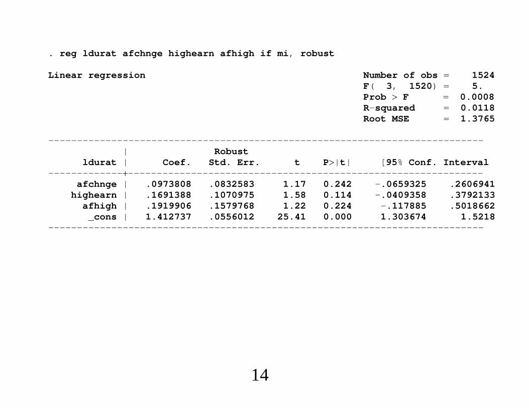
. reg ldurat afchnge highearn afhigh if mi, robust
Linear regression Number of obs 1524F( 3, 1520) 5.Prob F 0.0008R-squared 0.0118Root MSE 1.3765
----------------------------------------------------------------------------| Robust
ldurat | Coef. Std. Err. t P|t| [95% Conf. Interval---------------------------------------------------------------------------
afchnge | .0973808 .0832583 1.17 0.242 -.0659325 .2606941highearn | .1691388 .1070975 1.58 0.114 -.0409358 .3792133
afhigh | .1919906 .1579768 1.22 0.224 -.117885 .5018662_cons | 1.412737 .0556012 25.41 0.000 1.303674 1.5218
----------------------------------------------------------------------------
14
3. The Donald and Lang Approach∙ Donald and Lang (2007) propose a different perspective oninference when comparing differences among groups.∙ DL treat the problem as a small number of random drawsfrom a large population of clusters (because they assumeindependence across clusters).∙ A cluster-sampling problem but with small G.
15
∙ Simplest case: A single regressor that varies only bygroup:
ygm xg cg ugm
∙ DL focus on first equation, where cg is assumed to be
independent of xg with zero mean.
∙ So the DL criticism is not one of endogeneity of xg; it is
one of inference.
16

∙ DL highlight the problems of applying standard inferenceleaving cg as part of the error term, vgm cg ugm.
∙With actual cluster sampling, pooled OLS inference on
ygm xg cg ugm
can produce badly biased standard errors because it ignoresthe cluster correlation.
17
∙With a small G we cannot cluster. We cannot we cannotuse group fixed effects.∙ DL propose studying the regression in averages:
yg xg vg,g 1, . . . ,G.
∙ Add some strong assumptions:
Mg Mcg|xg Normal0,c2
ugm|xg,cg Normal0,u2
18
∙ Then
vg|xg Normal0,c2 u2/M
∙Model in averages satisfies the classical linear modelassumptions (we assume independent sampling across g).∙We can just use the “between” regression
yg on 1,xg,g 1, . . . ,G.
19
∙ The estimates of and are identical to pooled OLS
across g and m when Mg M for all g.
∙ Conditional on the xg, inherits its distribution from
vg : g 1, . . . ,G, the within-group averages of the
composite errors.∙ Inference can be based on the tG−2 distribution to testhypotheses about , provided G 2.
20

∙ So it is
tG−2 versus tM1M2MG−2
∙We can apply the DL method without normality of the ugmif the group sizes are large because Varvg c2 u2/Mg
so that ūg is a negligible part of vg. But we still need to
assume cg is normally distributed.
21
∙ If G 2 in the DL setting, we cannot do inference (thereare zero degrees of freedom).∙ Suppose xg is binary, indicating treatment and control
(g 2 is the treated, g 1 is the control).
∙ The DL estimate of is the usual one: y2 − y1. But we
cannot compute a standard error for .
∙ One way to see this is to write
y2 − y1 c2 − c1 ū2 − ū1
22
E|c1,c2 c2 − c1 ≡ a
Var|c1,c2 1
2
M12
2
M2
E
Var EVar|a VarE|a
1
2
M12
2
M2 a2
12
M12
2
M2 2c2
∙We cannot estimate c2.
23
∙ An implication of the DL framework is that the traditionaldifference-in-means approach to policy analysis cannot beused. Should we just give up when G 2?∙ In a sense the problem is an artifact of saying there arethree group-level parameters. If we write
ygm g xg ugm
where x1 0 and x2 1, then Ey1m 1 andEy2m 2 . There are only two means but three
parameters.
24
∙ The usual approach simply defines 1 Ey1m,
2 Ey2m, and then uses random samples from each
group to estimate the means. Any “cluster effect” isestimated as part of the mean.
25

∙ Applies to simple difference-in-differences settings withtwo periods of panel data.∙With G 2, let
ygm wgm2 − wgm1
be the change in a variable w from period one to two. Wehave a before period and an after period with a treated group(x2 1) and a control group (x1 0).
26

∙ The DL estimator of is the DD estimator:
Δw2 − Δw1
where Δw2 is the average of changes for the treament groupand Δw1 is the average change for the control.∙Well-known is the Card and Krueger (1994) minimumwage example. According to DL, cannot put a confidenceinterval around the estimated difference of employmentchanges.
27
∙ Even when the DL approach applies, should we use it?∙ Suppose G 4 with two control groups (x1 x2 0) andtwo treated groups (x3 x4 1).∙ DL involves the OLS regression yg on 1,xg, g 1, . . . , 4;
inference is based on the t2 distribution.
28
∙ Can show
y3 y4/2 − y1 y2/2.
∙ In the traditional setting, is approximately normal (for
almost any underlying population distributions) even withmoderate group sizes Mg.
29
∙ The DL approach essentially rejects usual inferencebecause it may not be the case that 1 2 and 3 4.
∙Why not allow heterogeneous means in the control andtreated groups?∙ Could just define the treatment effect as, say,
3 4/2 − 1 2/2,
and then plug in the unbiased, consistent, asymptoticallynormal estimators of the g under random sampling within
each g.
30

∙ Choice between traditional and DL approaches: Do wewant to estimate the effect with a fixed environment, orextrapolate to counterfactual scenarios?∙ Some schools are charter schools, others are not.Traditional inference takes the current assignments as given.∙ Can imagine reassigning the control and treatment groups(Donald and Lang).
31
Simulations∙ Sampling from fixed population or infinite population doesnot matter.∙ Fixed population results: Two control and two treatedgroups, with four different means fixed in the population.∙ Take 10 percent random samples (N 10,000), 1,000draws.∙ In one case keep the control and treatment groups fixed. Inthe other, reassign control and treatment with every newdraw.
32

∙ Traditional inference:reg y g1 g2 g3 g4, robust
lincom (g3 g4)/2 - (g1 g2)/2
∙ Donald and Lang:gen x g3 | g4
collapse y x, by(g)
reg y x
33
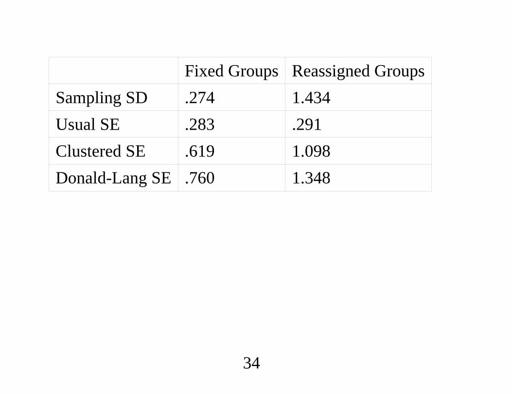
Fixed Groups Reassigned GroupsSampling SD .274 1.434Usual SE .283 .291Clustered SE .619 1.098Donald-Lang SE .760 1.348
34

4. Multiple Groups and Time Periods∙ Underlying model is a the individual level:
yigt t g xgt zigtgt vgt uigt,
i 1, . . . ,Mgt,
∙ Time effects, t, group effects, g.
∙ Policy variables xgt, individual-specific covariates, zigt,
unobserved group/time effects, vgt, and individual-specific
errors, uigt. Interested in .
35
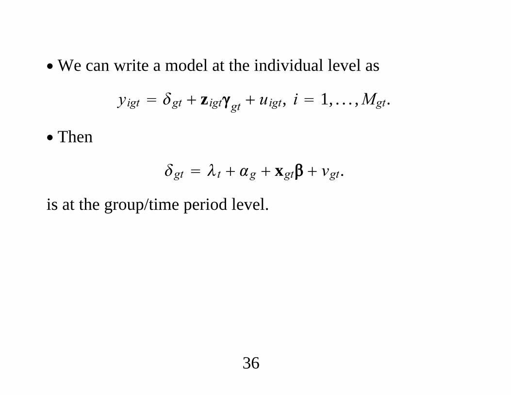
∙We can write a model at the individual level as
yigt gt zigtgt uigt, i 1, . . . ,Mgt.
∙ Then
gt t g xgt vgt.
is at the group/time period level.
36
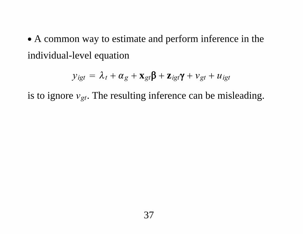
∙ A common way to estimate and perform inference in theindividual-level equation
yigt t g xgt zigt vgt uigt
is to ignore vgt. The resulting inference can be misleading.
37

∙ Bertrand, Duflo, and Mullainathan (2004) and Hansen(2007a) allow serial correlation in vgt : t 1,2, . . . ,T but
assume independence across g.∙We cannot replace t g a full set of group/time
interactions because that would eliminate xgt.
38

∙ If we view in gt t g xgt vgt as ultimately of
interest – which is usually the case because xgt contains the
aggregate policy variables – there are simple ways toproceed. We observe xgt, t is handled with year
dummies,and g just represents group dummies. The
problem, then, is that we do not observe gt.
39
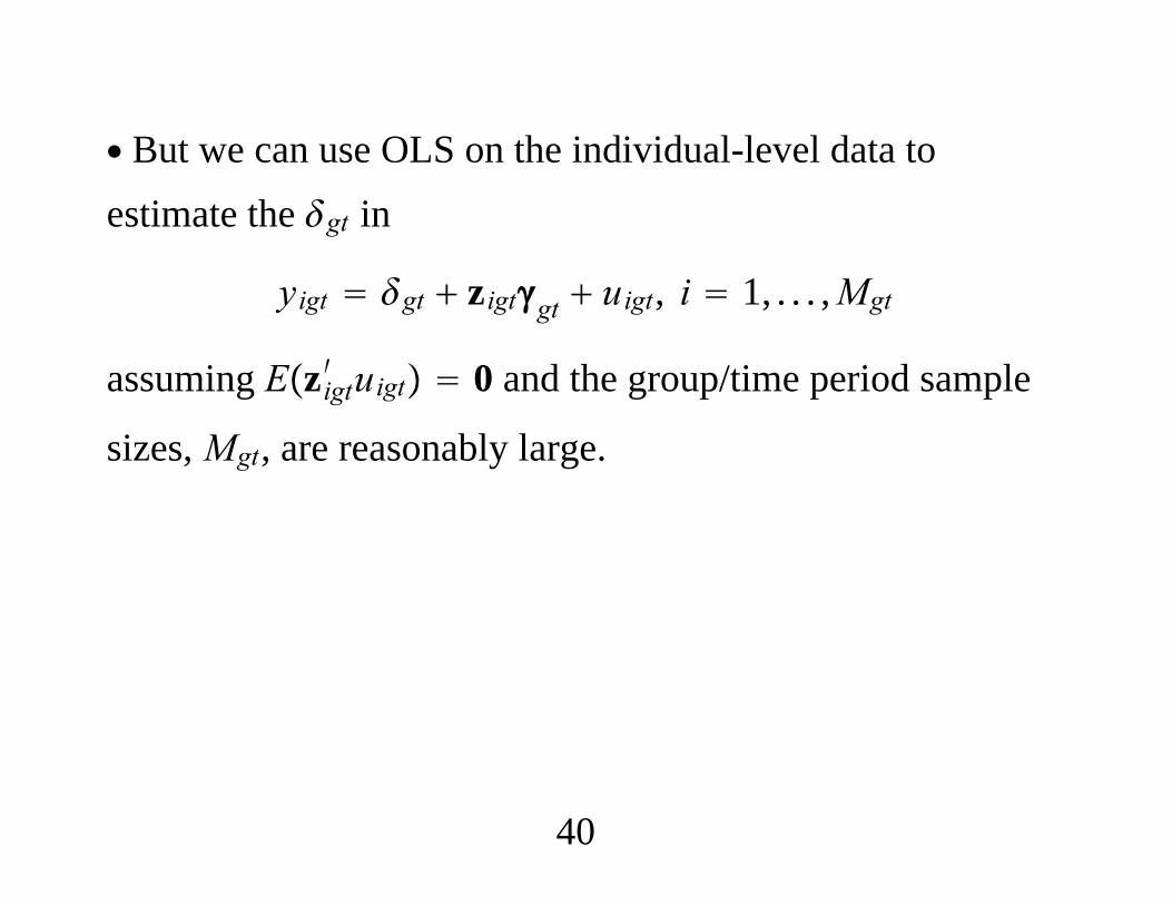
∙ But we can use OLS on the individual-level data toestimate the gt in
yigt gt zigtgt uigt, i 1, . . . ,Mgt
assuming Ezigt′ uigt 0 and the group/time period sample
sizes, Mgt, are reasonably large.
40
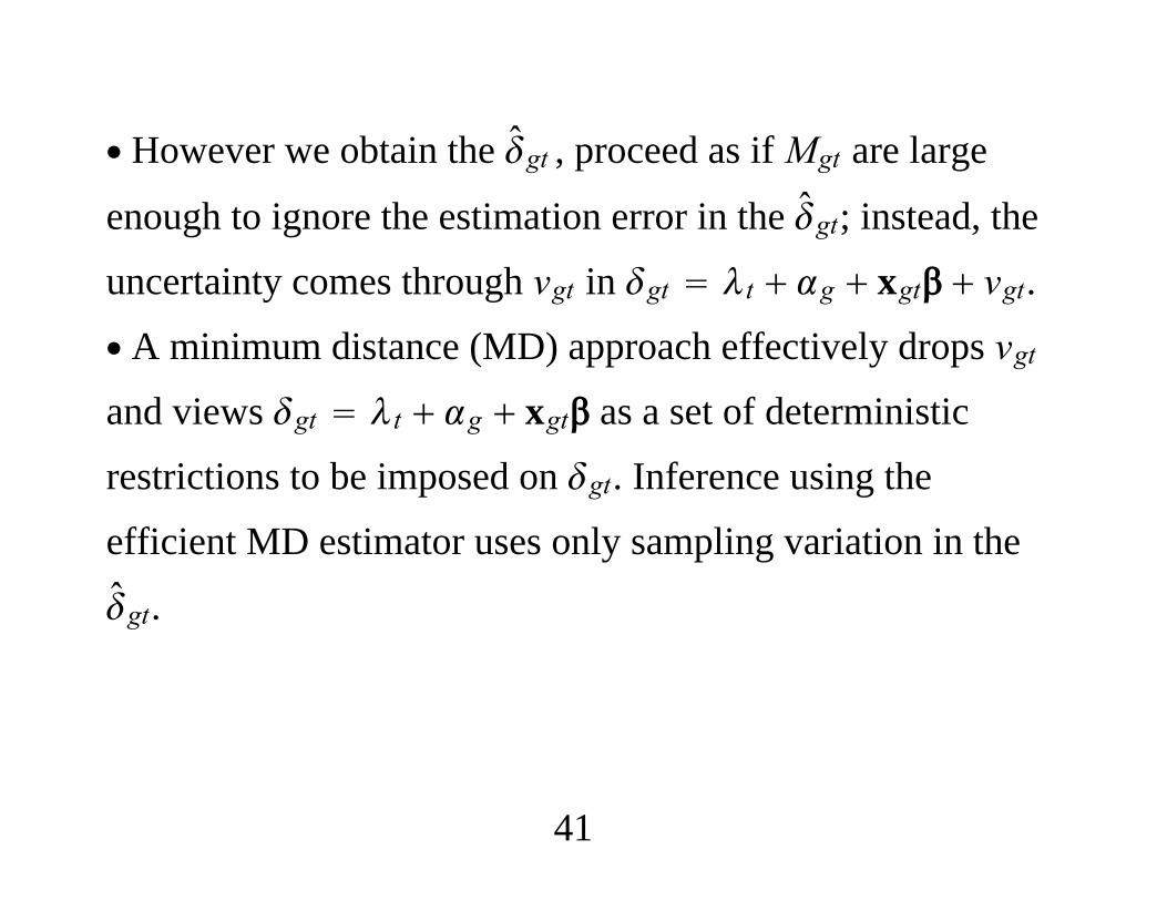
∙ However we obtain the gt , proceed as ifMgt are large
enough to ignore the estimation error in the gt; instead, the
uncertainty comes through vgt in gt t g xgt vgt.
∙ A minimum distance (MD) approach effectively drops vgtand views gt t g xgt as a set of deterministic
restrictions to be imposed on gt. Inference using the
efficient MD estimator uses only sampling variation in the
gt.
41

∙ Here, proceed ignoring estimation error, and act as if
gt t g xgt vgt.
∙We can apply the BDM findings and Hansen (2007a)results directly to this equation.∙ The OLS estimator and cluster-robust standard errors havegood large-sample properties as G and T both increase,provided vgt : t 1,2, . . . ,T is a weakly dependent time
series for all g.
42

5. Individual-Level Panel Data∙ Let wit be a binary indicator, which is unity if unit iparticipates in the program at time t. Consider
yit d2t wit ci uit, t 1,2,
where d2t 1 if t 2 and zero otherwise, ci is an observedeffect is the treatment effect.
43
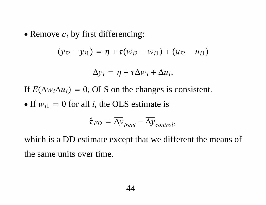
∙ Remove ci by first differencing:
yi2 − yi1 wi2 − wi1 ui2 − ui1
Δyi Δwi Δui.
If EΔwiΔui 0, OLS on the changes is consistent.∙ If wi1 0 for all i, the OLS estimate is
FD Δytreat − Δycontrol,
which is a DD estimate except that we different the means ofthe same units over time.
44
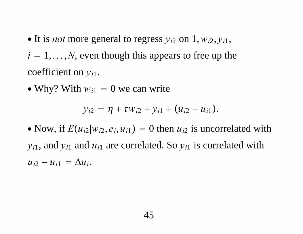
∙ It is not more general to regress yi2 on 1,wi2,yi1,i 1, . . . ,N, even though this appears to free up thecoefficient on yi1.∙Why? With wi1 0 we can write
yi2 wi2 yi1 ui2 − ui1.
∙ Now, if Eui2|wi2,ci,ui1 0 then ui2 is uncorrelated withyi1, and yi1 and ui1 are correlated. So yi1 is correlated withui2 − ui1 Δui.
45
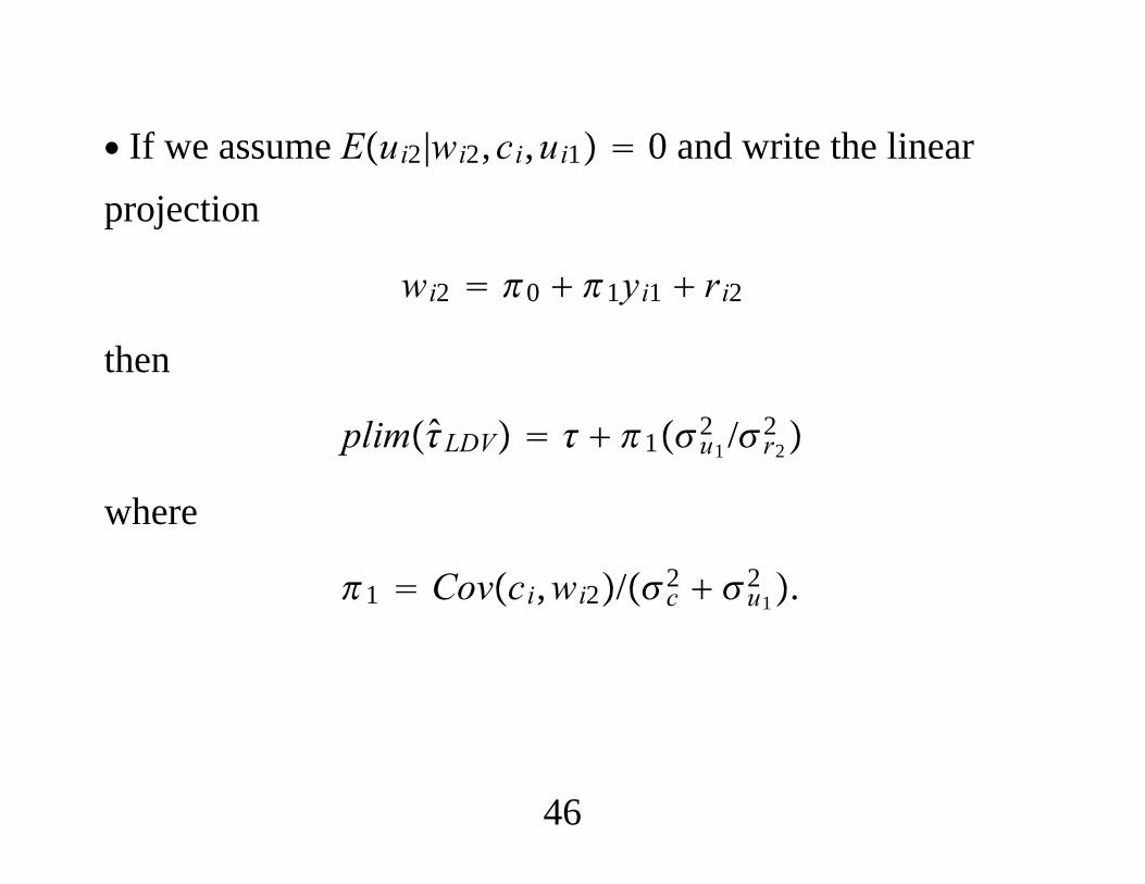
∙ If we assume Eui2|wi2,ci,ui1 0 and write the linearprojection
wi2 0 1yi1 ri2
then
plimLDV 1u12 /r22
where
1 Covci,wi2/c2 u12 .
46
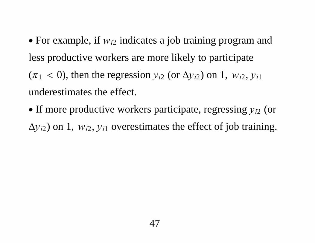
∙ For example, if wi2 indicates a job training program andless productive workers are more likely to participate(1 0), then the regression yi2 (or Δyi2) on 1, wi2, yi1underestimates the effect.∙ If more productive workers participate, regressing yi2 (orΔyi2) on 1, wi2, yi1 overestimates the effect of job training.
47
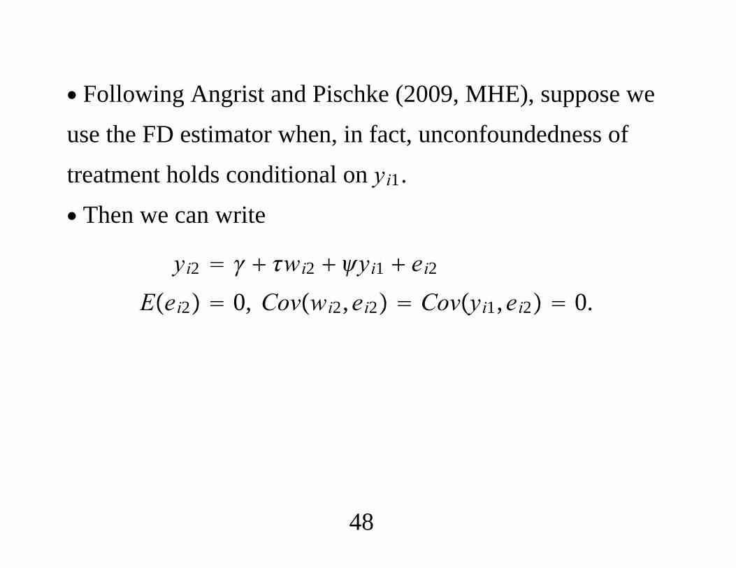
∙ Following Angrist and Pischke (2009, MHE), suppose weuse the FD estimator when, in fact, unconfoundedness oftreatment holds conditional on yi1.∙ Then we can write
yi2 wi2 yi1 ei2Eei2 0, Covwi2,ei2 Covyi1,ei2 0.
48
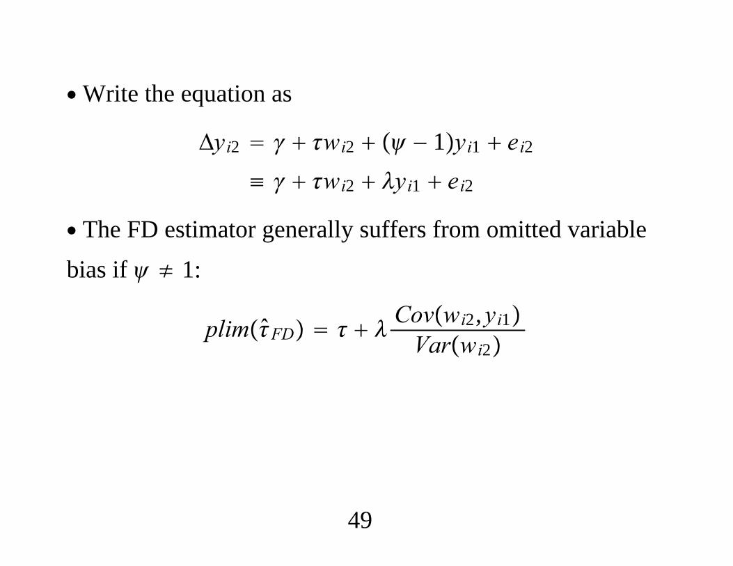
∙Write the equation as
Δyi2 wi2 − 1yi1 ei2≡ wi2 yi1 ei2
∙ The FD estimator generally suffers from omitted variablebias if ≠ 1:
plimFD Covwi2,yi1Varwi2
49
∙ If 0 ( 1) and Covwi2,yi1 0 – workers observed
with low first-period earnings are more likely to participate– the plimFD , and so FD overestimates the effect.∙We might expect to be close to unity for processes such
as earnings, which tend to be persistent. ( measures
persistence without conditioning on unobservedheterogeneity.)
50
∙ Algebraic fact: If 0 (as it usually will be even if 1) and wi2 and yi1 are negatively correlated in the
sample, FD LDV.
∙ If either is close to zero or wi2 and yi1 are weaklycorrelated, adding yi1 can have a small effect on the estimateof .
51

"Econometrics of Cross Section and Panel Data"
Lecture 12
Regression Discontinuity Designs:
New Developments and Practical Advice
Guido Imbens
Cemmap Lectures, UCL, June 2014

1. Introduction
2. Basics
3. Graphical Analyses
4. Local Linear Regression
5. Choosing the Bandwidth
6. Variance Estimation
7. External Validity
8. Specification Checks
1
What to Do and Not Do
1. Graphical Analyses: Non-smooth estimates of regression
functions of outcome on forcing variable.
2. Local linear/quadratic regression, not high order polyno-
mial regression.
3. Estimates of density of forcing variable to assess validity
4. Estimates of regression function of outcome on forcing vari-
able by treatment to assess external validity.
2
1. Introduction
A Regression Discontinuity (RD) Design is a powerful and
widely applicable identification strategy.
Often access to, or incentives for participation in, a service
or program is assigned based on transparent rules with crite-
ria based on clear cutoff values, rather than on discretion of
administrators.
Comparisons of individuals that are similar but on different sides
of the cutoff point can be credible estimates of causal effects
for a specific subpopulation.
Good for internal validity, but external validity is concern.
Long history in Psychology literature (Thistlewaite and Camp-
bell, 1960), early work by Goldberger (1972), recent resurgence
in economics.
3
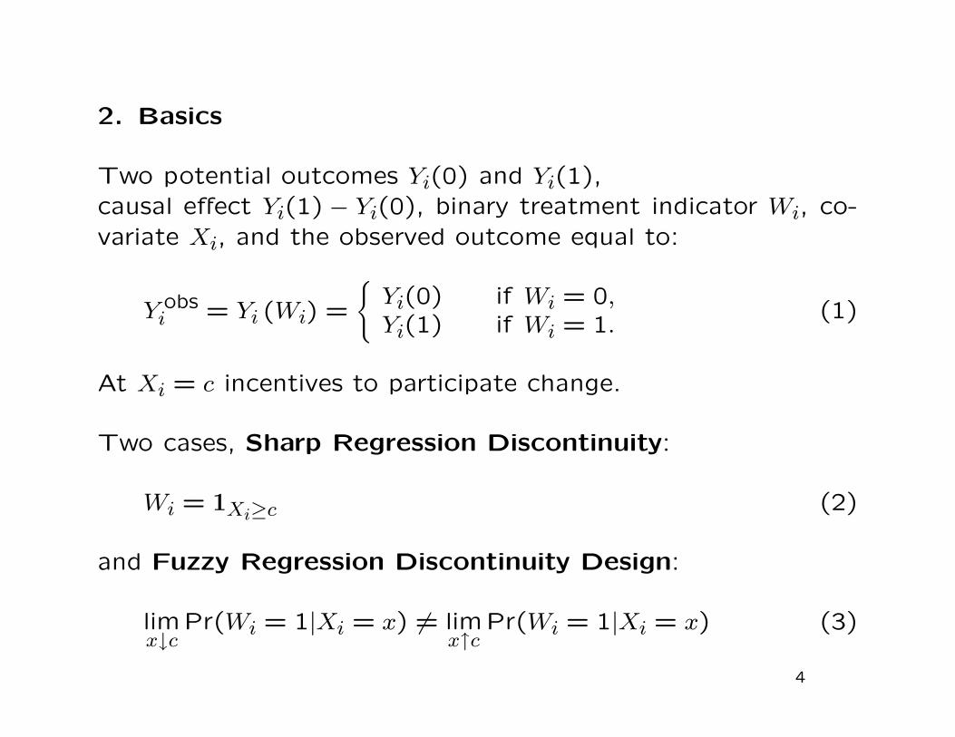
2. Basics
Two potential outcomes Yi(0) and Yi(1),
causal effect Yi(1) − Yi(0), binary treatment indicator Wi, co-
variate Xi, and the observed outcome equal to:
Y obsi = Yi (Wi) =
Yi(0) if Wi = 0,Yi(1) if Wi = 1.
(1)
At Xi = c incentives to participate change.
Two cases, Sharp Regression Discontinuity:
Wi = 1Xi≥c (2)
and Fuzzy Regression Discontinuity Design:
limx↓c
Pr(Wi = 1|Xi = x) 6= limx↑c
Pr(Wi = 1|Xi = x) (3)
4
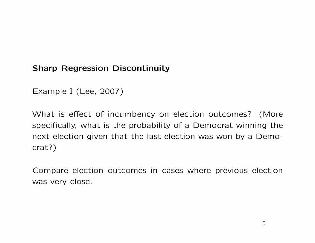
Sharp Regression Discontinuity
Example I (Lee, 2007)
What is effect of incumbency on election outcomes? (More
specifically, what is the probability of a Democrat winning the
next election given that the last election was won by a Demo-
crat?)
Compare election outcomes in cases where previous election
was very close.
5
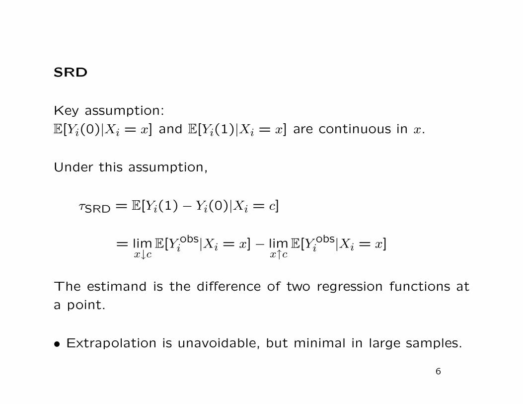
SRD
Key assumption:
E[Yi(0)|Xi = x] and E[Yi(1)|Xi = x] are continuous in x.
Under this assumption,
τSRD = E[Yi(1) − Yi(0)|Xi = c]
= limx↓c
E[Y obsi |Xi = x] − lim
x↑cE[Y obs
i |Xi = x]
The estimand is the difference of two regression functions at
a point.
• Extrapolation is unavoidable, but minimal in large samples.
6

Fuzzy Regression Discontinuity
Example II (VanderKlaauw, 2002)
What is effect of financial aid offer on acceptance of college
admission.
College admissions office puts applicants in a few categories
based on numerical score.
Financial aid offer is highly correlated with category.
Compare individuals close to cutoff score.
7

Example III, IV, Matsudaira (2008), Jacob and Lefgren (2004)
What is causal effect of participating in summer program on
test scores.
Summer program is mandatory for students who score below
a threshold on end-of-year tests. Not all students comply with
requirement.
Compare students close to threshold.
8
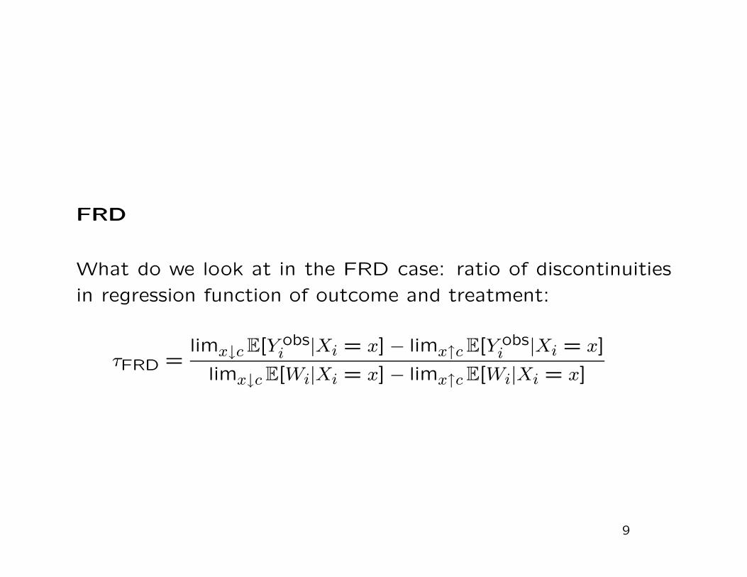
FRD
What do we look at in the FRD case: ratio of discontinuities
in regression function of outcome and treatment:
τFRD =limx↓c E[Y obs
i |Xi = x] − limx↑c E[Y obsi |Xi = x]
limx↓c E[Wi|Xi = x] − limx↑c E[Wi|Xi = x]
9
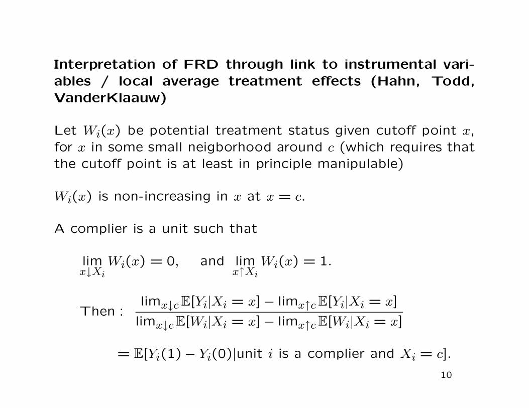
Interpretation of FRD through link to instrumental vari-
ables / local average treatment effects (Hahn, Todd,
VanderKlaauw)
Let Wi(x) be potential treatment status given cutoff point x,
for x in some small neigborhood around c (which requires that
the cutoff point is at least in principle manipulable)
Wi(x) is non-increasing in x at x = c.
A complier is a unit such that
limx↓Xi
Wi(x) = 0, and limx↑Xi
Wi(x) = 1.
Then :limx↓c E[Yi|Xi = x] − limx↑c E[Yi|Xi = x]
limx↓c E[Wi|Xi = x] − limx↑c E[Wi|Xi = x]
= E[Yi(1)− Yi(0)|unit i is a complier and Xi = c].
10
3. Graphical Analyses
A. Plot regression function E[Y obsi |Xi = x] for assessing effect
of treatment and validity
B. Plot regression function E[Wi|Xi = x] (for fuzzy rd’s) for
assessing strength of design
C. Plot regression functions E[Zi|Xi = x] for covariates Zi that
do not enter in the assignment rule for assessing validity
D. Plot density fX(x) for assessing validity.
In all cases use estimators that do not smooth everywhere.
For example, use bins and average outcomes within bins.
11

−1 −0.8 −0.6 −0.4 −0.2 0 0.2 0.4 0.6 0.8 10
0.1
0.2
0.3
0.4
0.5
0.6
0.7
0.8
0.9
1Fig 1: Regression Function for Democratic Vote Share, Lee Congressional Vote Data
difference in vote share last election
dem
ocra
tic v
ote
shar
e

1 1.5 2 2.5 3 3.5 4 4.5 5 5.50
0.2
0.4
0.6
0.8
1Fig 2: Jacob, Regression Function for Participation
initial reading score
sum
mer
sch
ool p
artic
ipat
ion
1 1.5 2 2.5 3 3.5 4 4.5 5 5.5−4
−3
−2
−1
0
1
2
3
4Fig 3: Regression Function for Math Score
initial reading score
final
mat
h sc
ore

−1 −0.8 −0.6 −0.4 −0.2 0 0.2 0.4 0.6 0.8 10
0.1
0.2
0.3
0.4
0.5
0.6
0.7
0.8
0.9
1Fig 4: Regression Function for Democratic Vote Share in Previous Election, Lee Congressional Vote Data
difference in vote share last election
dem
ocra
tic v
ote
shar
e in
pre
viou
s el
ectio
n

−1 −0.8 −0.6 −0.4 −0.2 0 0.2 0.4 0.6 0.8 10
0.2
0.4
0.6
0.8
1
1.2
1.4
1.6
1.8Fig 5: Density for Forcing Variable
difference in vote share last election
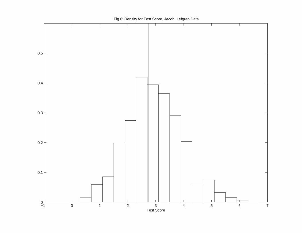
−1 0 1 2 3 4 5 6 70
0.1
0.2
0.3
0.4
0.5
Fig 6: Density for Test Score, Jacob−Lefgren Data
Test Score

4. Estimation: Local Linear Regression
We are interested in the value of a regression function at the
boundary of the support.
Do not use standard kernel regression
µl(c) =N∑
i|c−h<Xi<c
Yi
/ N∑
i|c−h<Xi<c
1
This does not work well for that case (slower convergence
rates) because we estimate regression functions at the bound-
ary of the support.
12
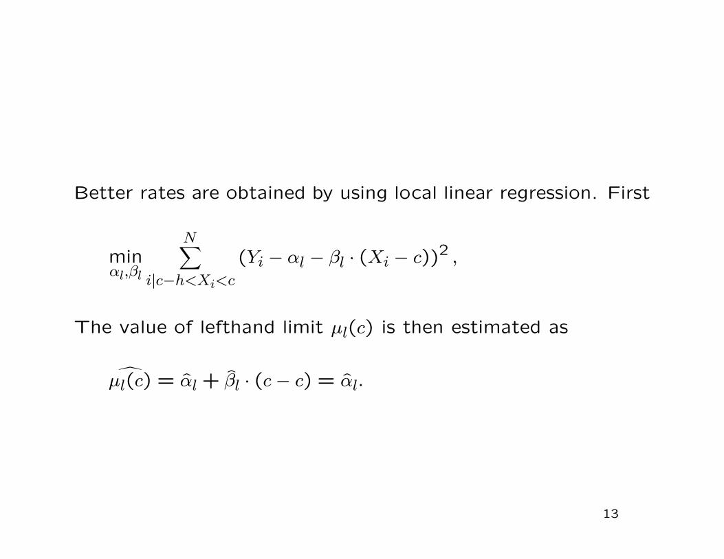
Better rates are obtained by using local linear regression. First
minαl,βl
N∑
i|c−h<Xi<c
(Yi − αl − βl · (Xi − c))2 ,
The value of lefthand limit µl(c) is then estimated as
µl(c) = αl + βl · (c − c) = αl.
13
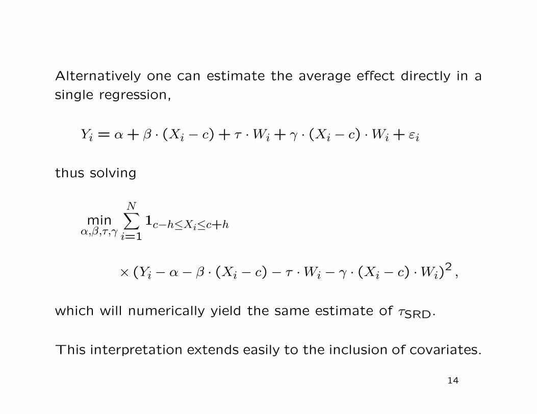
Alternatively one can estimate the average effect directly in a
single regression,
Yi = α + β · (Xi − c) + τ · Wi + γ · (Xi − c) · Wi + εi
thus solving
minα,β,τ,γ
N∑
i=1
1c−h≤Xi≤c+h
× (Yi − α − β · (Xi − c) − τ · Wi − γ · (Xi − c) · Wi)2 ,
which will numerically yield the same estimate of τSRD.
This interpretation extends easily to the inclusion of covariates.
14
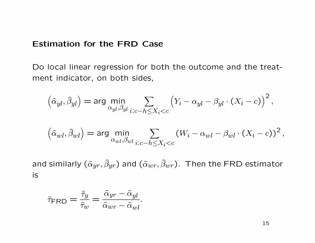
Estimation for the FRD Case
Do local linear regression for both the outcome and the treat-
ment indicator, on both sides,
(αyl, βyl
)= arg min
αyl,βyl
∑
i:c−h≤Xi<c
(Yi − αyl − βyl · (Xi − c)
)2,
(αwl, βwl
)= arg min
αwl,βwl
∑
i:c−h≤Xi<c
(Wi − αwl − βwl · (Xi − c))2 ,
and similarly (αyr, βyr) and (αwr, βwr). Then the FRD estimator
is
τFRD =τy
τw=
αyr − αyl
αwr − αwl.
15
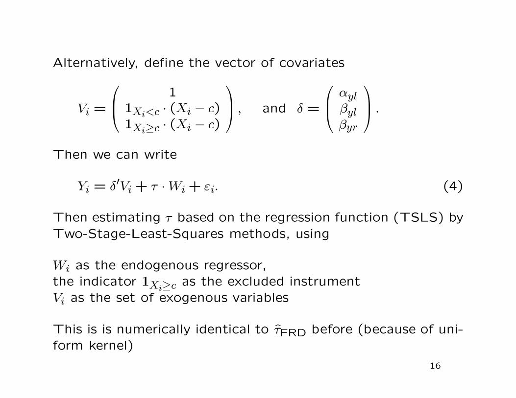
Alternatively, define the vector of covariates
Vi =
11Xi<c · (Xi − c)1Xi≥c · (Xi − c)
, and δ =
αylβylβyr
.
Then we can write
Yi = δ′Vi + τ · Wi + εi. (4)
Then estimating τ based on the regression function (TSLS) by
Two-Stage-Least-Squares methods, using
Wi as the endogenous regressor,
the indicator 1Xi≥c as the excluded instrument
Vi as the set of exogenous variables
This is is numerically identical to τFRD before (because of uni-
form kernel)
16
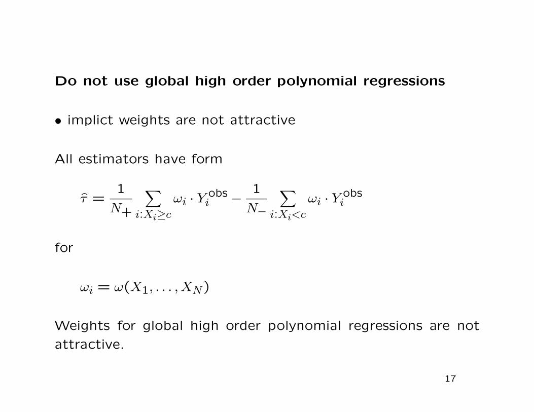
Do not use global high order polynomial regressions
• implict weights are not attractive
All estimators have form
τ =1
N+
∑
i:Xi≥c
ωi · Y obsi − 1
N−
∑
i:Xi<c
ωi · Y obsi
for
ωi = ω(X1, . . . , XN)
Weights for global high order polynomial regressions are not
attractive.
17
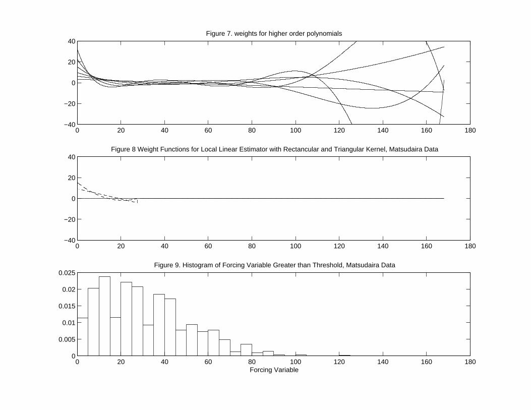
0 20 40 60 80 100 120 140 160 180−40
−20
0
20
40Figure 8 Weight Functions for Local Linear Estimator with Rectancular and Triangular Kernel, Matsudaira Data
0 20 40 60 80 100 120 140 160 180−40
−20
0
20
40Figure 7. weights for higher order polynomials
0 20 40 60 80 100 120 140 160 1800
0.005
0.01
0.015
0.02
0.025
Forcing Variable
Figure 9. Histogram of Forcing Variable Greater than Threshold, Matsudaira Data

• global high order polynomial estimates are sensitive to order
of polynomial.
Matsudaira Data - Estimates of Effect of Summer Program
order of polynomial estimates se
global 1 0.167 (0.008)global 2 -0.079 (0.010)global 3 -0.112 (0.011)global 4 -0.077 (0.013)global 5 -0.069 (0.016)global 6 -0.104 (0.018)
local 1 -0.080 (0.012)local 2 -0.063 (0.017)
18
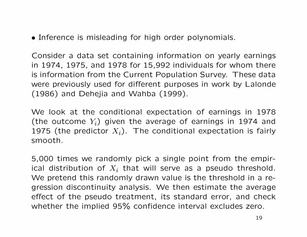
• Inference is misleading for high order polynomials.
Consider a data set containing information on yearly earnings
in 1974, 1975, and 1978 for 15,992 individuals for whom there
is information from the Current Population Survey. These data
were previously used for different purposes in work by Lalonde
(1986) and Dehejia and Wahba (1999).
We look at the conditional expectation of earnings in 1978
(the outcome Yi) given the average of earnings in 1974 and
1975 (the predictor Xi). The conditional expectation is fairly
smooth.
5,000 times we randomly pick a single point from the empir-
ical distribution of Xi that will serve as a pseudo threshold.
We pretend this randomly drawn value is the threshold in a re-
gression discontinuity analysis. We then estimate the average
effect of the pseudo treatment, its standard error, and check
whether the implied 95% confidence interval excludes zero.
19

0 5 10 15 20 250
5
10
15
20
25Fig 10: Lalonde Data, Regression of Earnings in 1978 on Average of Earnings in 1974, 1975
Average of Earnings in 1974, 1975
Ear
ning
s in
197
8
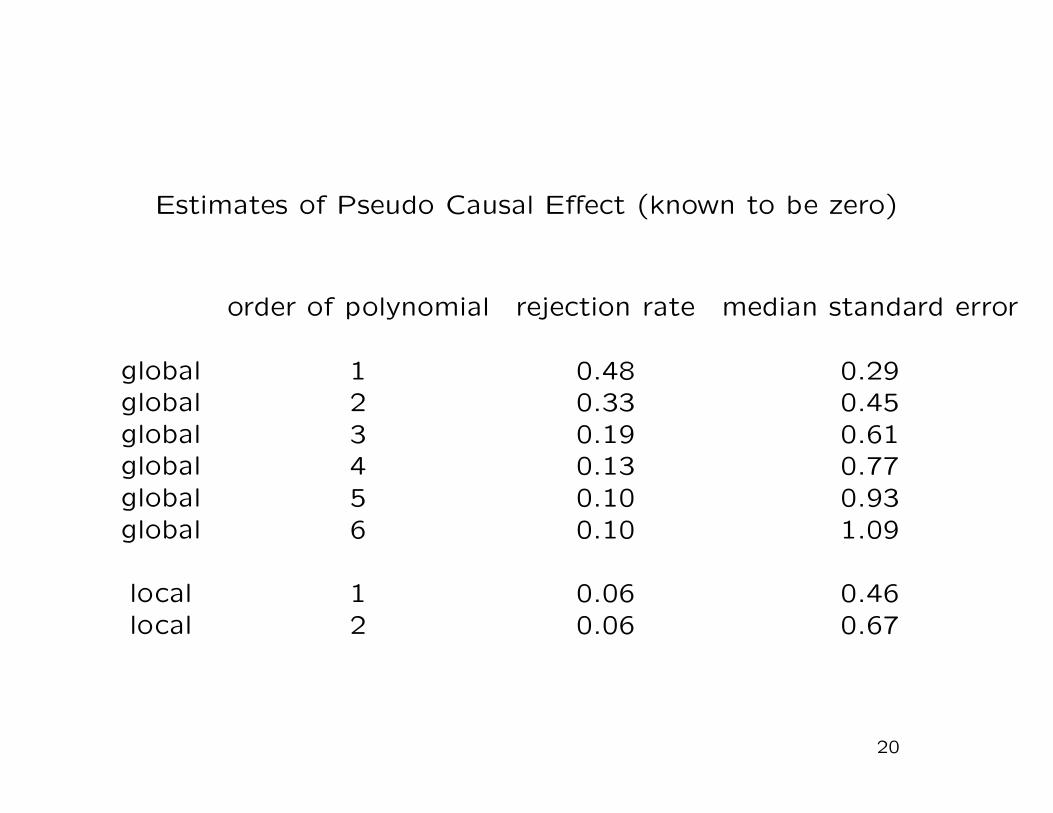
Estimates of Pseudo Causal Effect (known to be zero)
order of polynomial rejection rate median standard error
global 1 0.48 0.29global 2 0.33 0.45global 3 0.19 0.61global 4 0.13 0.77global 5 0.10 0.93global 6 0.10 1.09
local 1 0.06 0.46local 2 0.06 0.67
20

5. Choosing the Bandwidth (Imbens-Kalyanaraman)
We wish to take into account that (i) we are interested in the
regression function at the boundary of the support, and (ii)
that we are interested in the regression function at x = c.
IK focus on minimizing
E[(µl(c) − µl(c))
2 + (µr(c) − µr(c))2]
Both µl(c) and µr(c) are based on local linear estimators, with
the same bandwidth h.
21
Optimal Bandwidth
hopt =
(C2
C1
)1/5
·
σ2r (c)
p·fr(c)+
σ2l (c)
(1−p)·fl(c)(∂2mr∂x2 (c)
)2+
(∂2ml∂x2 (c)
)2
1/5
· N−1/5
p is share of observations above threshold.
C1 =1
4·(
ν22 − ν1ν3
ν2ν0 − ν21
)2
C2 =
∫∞0 (ν2 − uν1))
2 K2(u)du(ν2ν0 − ν2
1
)2
νj =∫ ∞
0ujK(u)du
If K(u) = 1|u|<0.5, then (C2/C1) = 5.40
22

Bandwidth for FRD Design
1. Calculate optimal bandwidth separately for both regression
functions and choose smallest.
2. Calculate optimal bandwidth only for outcome and use that
for both regression functions.
Typically the regression function for the treatment indicator
is flatter than the regression function for the outcome away
from the discontinuity point (completely flat in the SRD case).
So using same criterion would lead to larger bandwidth for
estimation of regression function for treatment indicator. In
practice it is easier to use the same bandwidth, and so to
23

avoid bias, use the bandwidth from criterion for SRD design or
smallest.
Cattaneo et al (2014) suggest using this bandwidth with a local
quadratic to improve coverage properties.
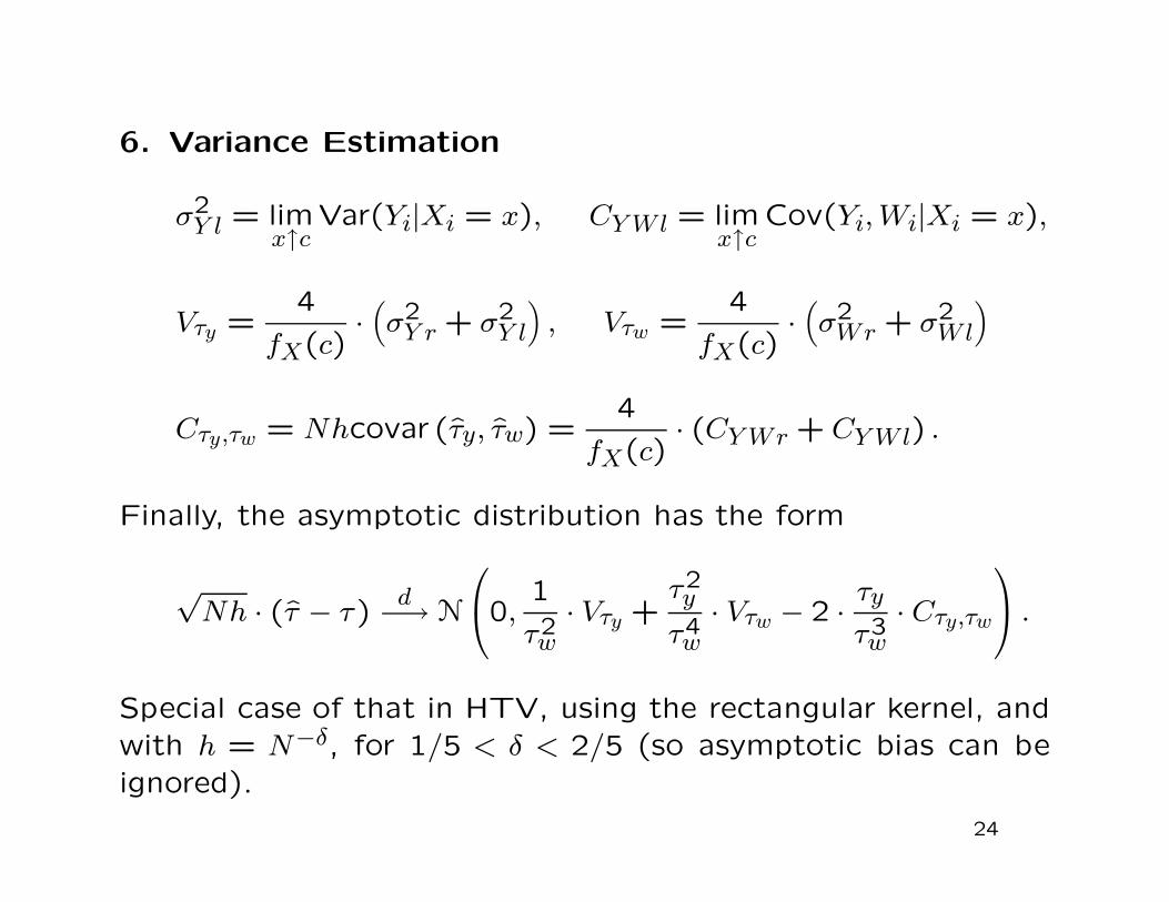
6. Variance Estimation
σ2Y l = lim
x↑cVar(Yi|Xi = x), CY Wl = lim
x↑cCov(Yi, Wi|Xi = x),
Vτy =4
fX(c)·(σ2
Y r + σ2Y l
), Vτw =
4
fX(c)·(σ2
Wr + σ2Wl
)
Cτy,τw = Nhcovar (τy, τw) =4
fX(c)· (CY Wr + CY Wl) .
Finally, the asymptotic distribution has the form
√Nh · (τ − τ)
d−→ N
0,
1
τ2w· Vτy +
τ2y
τ4w· Vτw − 2 · τy
τ3w· Cτy,τw
.
Special case of that in HTV, using the rectangular kernel, and
with h = N−δ, for 1/5 < δ < 2/5 (so asymptotic bias can be
ignored).
24
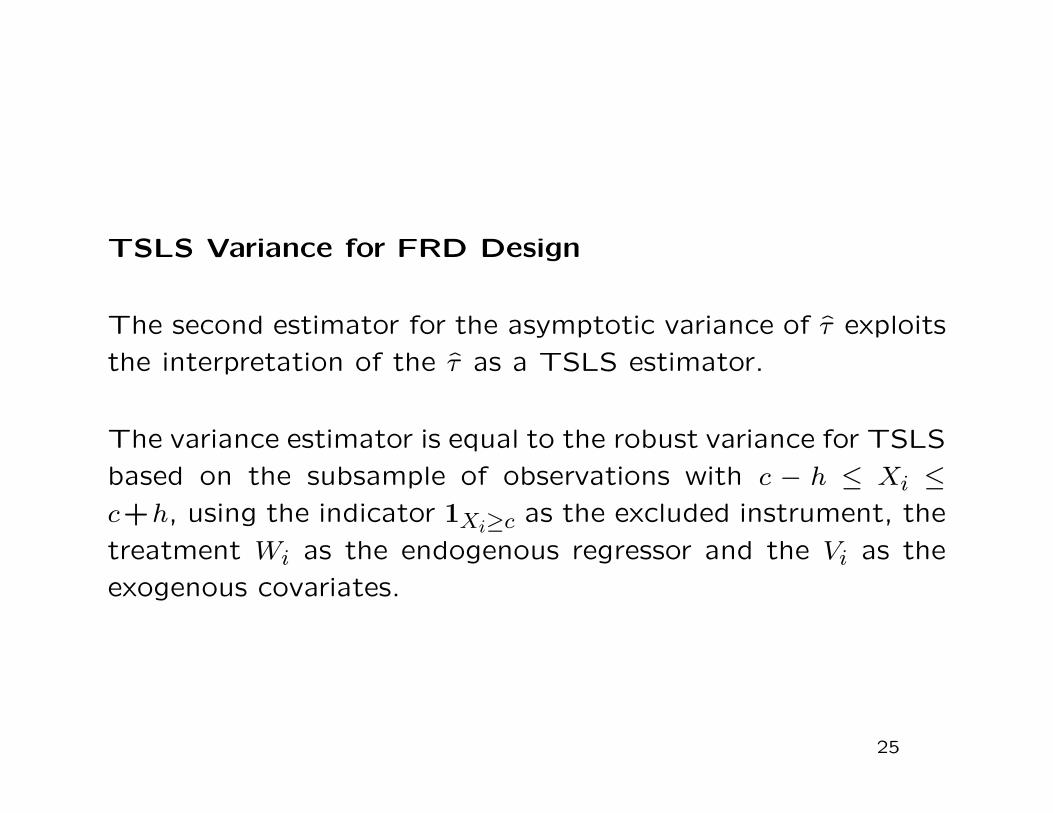
TSLS Variance for FRD Design
The second estimator for the asymptotic variance of τ exploits
the interpretation of the τ as a TSLS estimator.
The variance estimator is equal to the robust variance for TSLS
based on the subsample of observations with c − h ≤ Xi ≤c+h, using the indicator 1Xi≥c as the excluded instrument, the
treatment Wi as the endogenous regressor and the Vi as the
exogenous covariates.
25

7. External Validity
The estimand has little external validity. It is at best valid for
a population defined by the cutoff value c, and by the complier
subpopulation that is affected at that value.
26

FRD versus Unconfoundedness
Yi(0), Yi(1) ⊥⊥ Wi | Xi. (5)
Under this assumption:
E[Yi(1)− Yi(0)|Xi = c] = E[Yi|Wi = 1,Xi = c]− E[Yi|Wi = 0,Xi = c].
This approach assumes that differences between treated and
control units with Xi = c have a causal interpretation, without
exploiting the discontinuity. Unconfoundedness is based on
units being comparable if their covariates are similar. This is
not an attractive assumption in the current setting where the
probability of receiving the treatment is discontinuous in the
covariate.
Even if unconfoundedness holds, under continuity of potential
outcome regression functions FRD approach will be consistent
for the average effect for compliers at Xi = c.
27
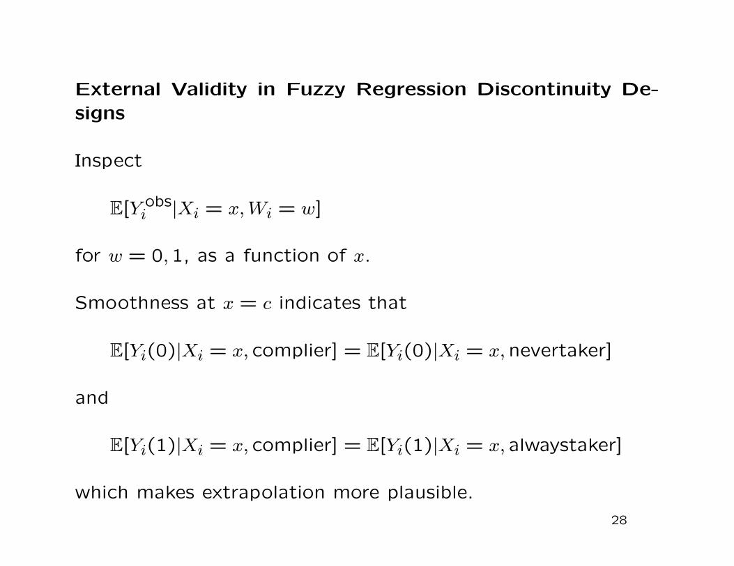
External Validity in Fuzzy Regression Discontinuity De-
signs
Inspect
E[Y obsi |Xi = x, Wi = w]
for w = 0,1, as a function of x.
Smoothness at x = c indicates that
E[Yi(0)|Xi = x, complier] = E[Yi(0)|Xi = x, nevertaker]
and
E[Yi(1)|Xi = x, complier] = E[Yi(1)|Xi = x, alwaystaker]
which makes extrapolation more plausible.
28
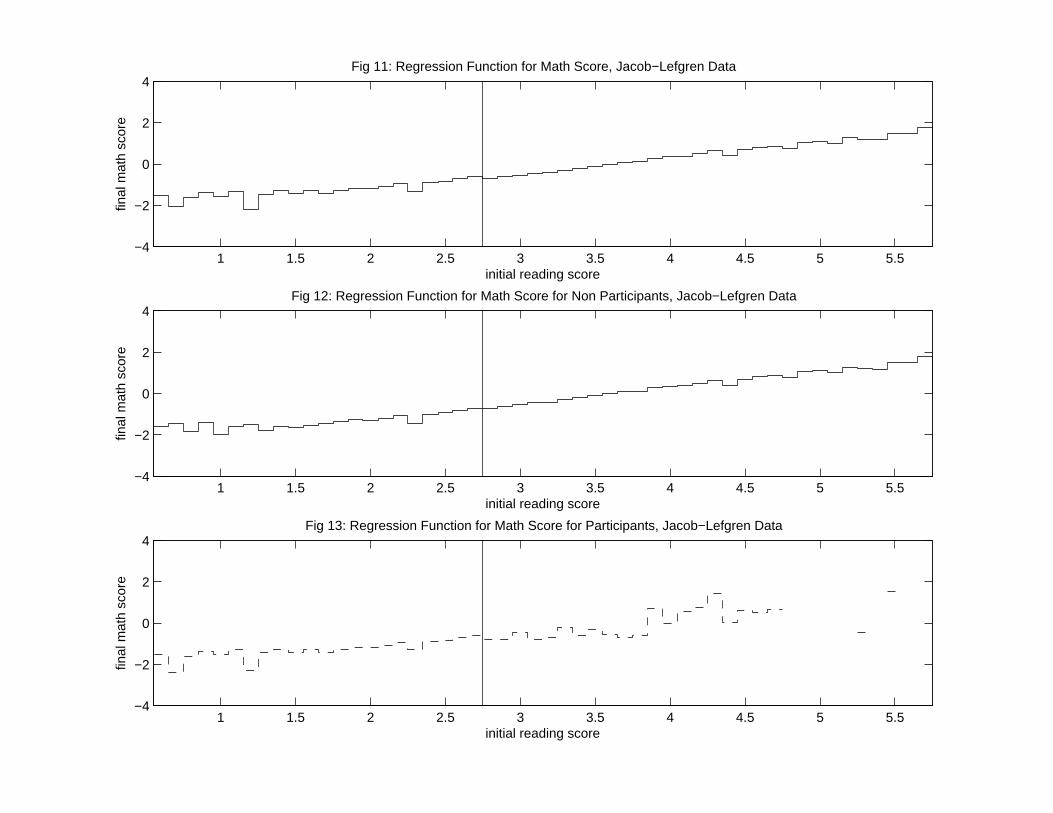
1 1.5 2 2.5 3 3.5 4 4.5 5 5.5−4
−2
0
2
4Fig 11: Regression Function for Math Score, Jacob−Lefgren Data
initial reading score
final
mat
h sc
ore
1 1.5 2 2.5 3 3.5 4 4.5 5 5.5−4
−2
0
2
4Fig 12: Regression Function for Math Score for Non Participants, Jacob−Lefgren Data
initial reading score
final
mat
h sc
ore
1 1.5 2 2.5 3 3.5 4 4.5 5 5.5−4
−2
0
2
4Fig 13: Regression Function for Math Score for Participants, Jacob−Lefgren Data
initial reading score
final
mat
h sc
ore
8. Concerns about Validity
Two main conceptual concerns in the application of RD de-
signs, sharp or fuzzy.
Other Changes
Possibility of other changes at the same cutoff value of the
covariate. Such changes may affect the outcome, and these
effects may be attributed erroneously to the treatment of
interest.
Manipulation of Forcing Variable
The second concern is that of manipulation of the covariate
value.
29

Specification Checks
A. Discontinuities in Average Covariates
B. A Discontinuity in the Distribution of the Forcing Variable
C. Discontinuities in Average Outcomes at Other Values
D. Sensitivity to Bandwidth Choice
30

8.A Discontinuities in Average Covariates
Test the null hypothesis of a zero average effect on pseudo
outcomes known not to be affected by the treatment.
Such variables includes covariates that are by definition not
affected by the treatment. Such tests are familiar from settings
with identification based on unconfoundedness assumptions.
Although not required for the validity of the design, in most
cases, the reason for the discontinuity in the probability of the
treatment does not suggest a discontinuity in the average value
of covariates. If we find such a discontinuity, it typically casts
doubt on the assumptions underlying the RD design.
31

8.B A Discontinuity in the Distribution of the Forcing
Variable
McCrary (2007) suggests testing the null hypothesis of conti-
nuity of the density of the covariate that underlies the assign-
ment at the discontinuity point, against the alternative of a
jump in the density function at that point.
Again, in principle, the design does not require continuity of the
density of X at c, but a discontinuity is suggestive of violations
of the no-manipulation assumption.
If in fact individuals partly manage to manipulate the value of
X in order to be on one side of the boundary rather than the
other, one might expect to see a discontinuity in this density
at the discontinuity point.
32

8.C Discontinuities in Avareage Outcomes at Other Val-
ues
Taking the subsample with Xi < c we can test for a jump in the
conditional mean of the outcome at the median of the forcing
variable.
To implement the test, use the same method for selecting the
binwidth as before. Also estimate the standard errors of the
jump and use this to test the hypothesis of a zero jump.
Repeat this using the subsample to the right of the cutoff point
with Xi ≥ c. Now estimate the jump in the regression function
and at qX,1/2,r, and test whether it is equal to zero.
33
8.D Sensitivity to Bandwidth Choice
One should investigate the sensitivity of the inferences to this
choice, for example, by including results for bandwidths twice
(or four times) and half (or a quarter of) the size of the origi-
nally chosen bandwidth.
Obviously, such bandwidth choices affect both estimates and
standard errors, but if the results are critically dependent on a
particular bandwidth choice, they are clearly less credible than
if they are robust to such variation in bandwidths.
34

"Econometrics of Cross Section and Panel Data"
Lecture 13
Bayesian Inference
Guido Imbens
Cemmap Lectures, UCL, June 2014

Outline
1. Introduction
2. Basics
3. Bernstein-Von Mises Theorem
4. Markov-Chain-Monte-Carlo Methods
5. Example: Demand Models with Unobs Heterog in Prefer.
6. Example: Panel Data with Multiple Individual Specific Param.
1
7. Instrumental Variables with Many Instruments
8. Example: Binary Response with Endogenous Regressors
9. Example: Discrete Choice Models with Unobserved Choice
Characteristics

1. Introduction
Formal Bayesian methods surprisingly rarely used in empirical
work in economics.
Surprising, because they are attractive options in many set-
tings, especially with many parameters (like random coefficient
models), when large sample normal approximations are not ac-
curate. (see examples below)
In cases where large sample normality does not hold, frequentist
methods are sometimes awkward (e.g, confidence intervals that
can be empty, such as in unit root or weak instrument cases).
Bayesian approach allows for conceptually straightforward way
of dealing with unit-level heterogeneity in preferences/parameters.
2
Why are Bayesian methods not used more widely?
1. choice of methods does not matter (bernstein-von mises
theorem)
2. difficulty in specifying prior distribution (not “objective”)
3. need for fully parametric model
4. computational difficulties
3
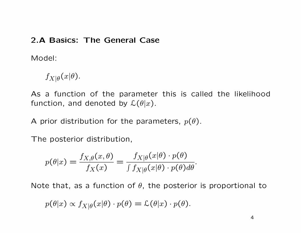
2.A Basics: The General Case
Model:
fX|θ(x|θ).
As a function of the parameter this is called the likelihood
function, and denoted by L(θ|x).
A prior distribution for the parameters, p(θ).
The posterior distribution,
p(θ|x) =fX,θ(x, θ)
fX(x)=
fX|θ(x|θ) · p(θ)∫
fX|θ(x|θ) · p(θ)dθ.
Note that, as a function of θ, the posterior is proportional to
p(θ|x) ∝ fX|θ(x|θ) · p(θ) = L(θ|x) · p(θ).4

2.B Example: The Normal Case
Suppose the conditional distribution of X given the parameter
µ is N(µ,1).
Suppose the prior distribution for µ to be N(0,100).
The posterior distribution is proportional to
fµ|X(µ|x) ∝ exp
(
−1
2(x − µ)2
)
· exp(
− 1
2 · 100µ2)
= exp−1
2(x2 − 2xµ + µ2 + µ2/100)
∝ exp(− 1
2(100/101)(µ − (100/101)x)2)
∼ N(x · 100/101,100/101)
5
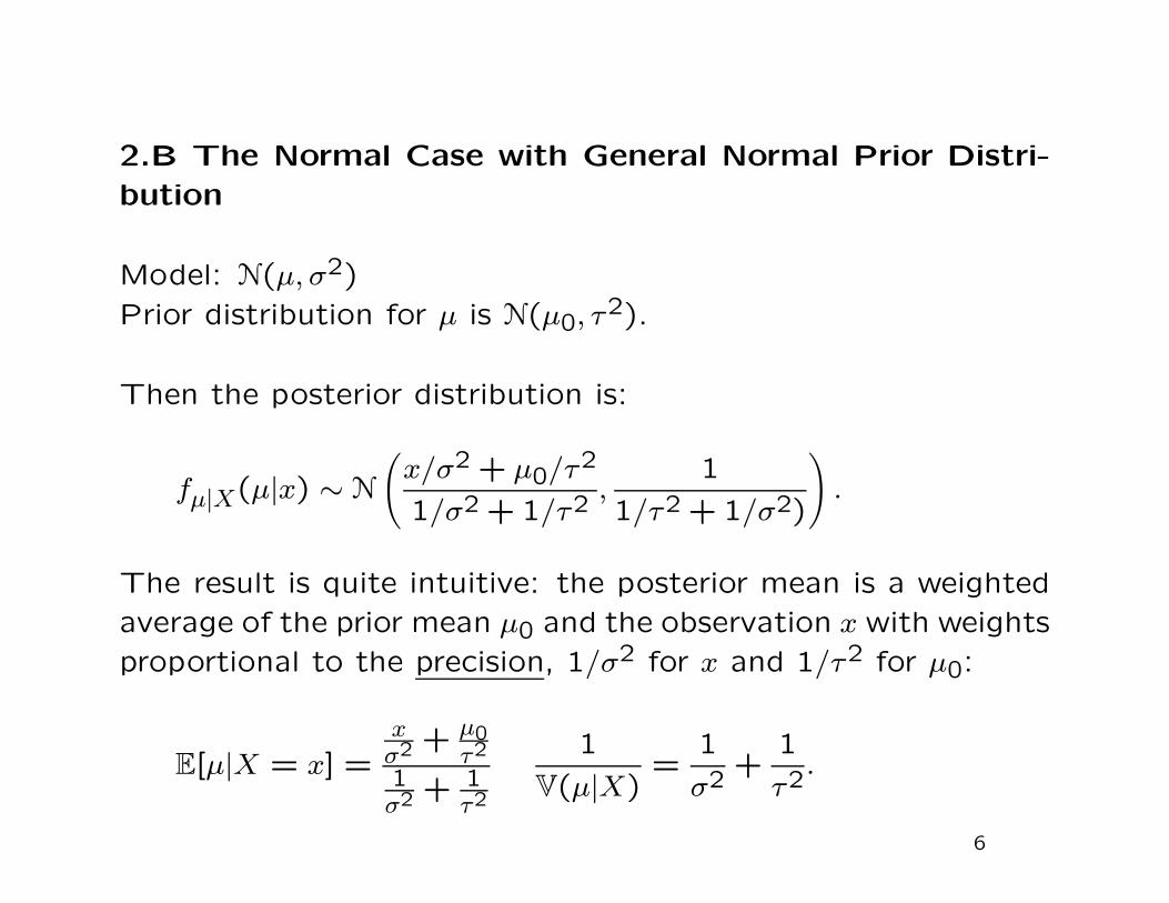
2.B The Normal Case with General Normal Prior Distri-
bution
Model: N(µ, σ2)
Prior distribution for µ is N(µ0, τ2).
Then the posterior distribution is:
fµ|X(µ|x) ∼ N
(
x/σ2 + µ0/τ2
1/σ2 + 1/τ2,
1
1/τ2 + 1/σ2)
)
.
The result is quite intuitive: the posterior mean is a weighted
average of the prior mean µ0 and the observation x with weights
proportional to the precision, 1/σ2 for x and 1/τ2 for µ0:
E[µ|X = x] =
xσ2 + µ0
τ2
1σ2 + 1
τ2
1
V(µ|X)=
1
σ2+
1
τ2.
6

Suppose we are really sure about the value of µ before we
conduct the experiment. In that case we would set τ2 small
and the weight given to the observation would be small, and the
posterior distribution would be close to the prior distribution.
Suppose on the other hand we are very unsure about the value
of µ. What value for τ should we choose? We can let τ go
to infinity. Even though the prior distribution is not a proper
distribution anymore if τ2 = ∞, the posterior distribution is
perfectly well defined, namely µ|X ∼ N(X, σ2).
In that case we have an improper prior distribution. We give
equal prior weight to any value of µ (flat prior). That would
seem to capture pretty well the idea that a priori we are ignorant
about µ.
This is not always easy to do. For example, a flat prior distri-
bution is not always uninformative about particular functions
of parameters.
7
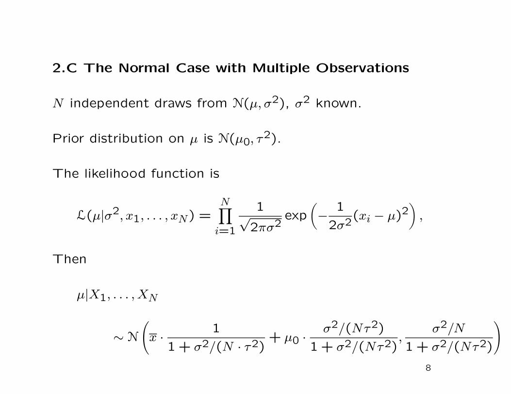
2.C The Normal Case with Multiple Observations
N independent draws from N(µ, σ2), σ2 known.
Prior distribution on µ is N(µ0, τ2).
The likelihood function is
L(µ|σ2, x1, . . . , xN) =N∏
i=1
1√2πσ2
exp
(
− 1
2σ2(xi − µ)2
)
,
Then
µ|X1, . . . , XN
∼ N
(
x · 1
1 + σ2/(N · τ2)+ µ0 · σ2/(Nτ2)
1 + σ2/(Nτ2),
σ2/N
1 + σ2/(Nτ2)
)
8
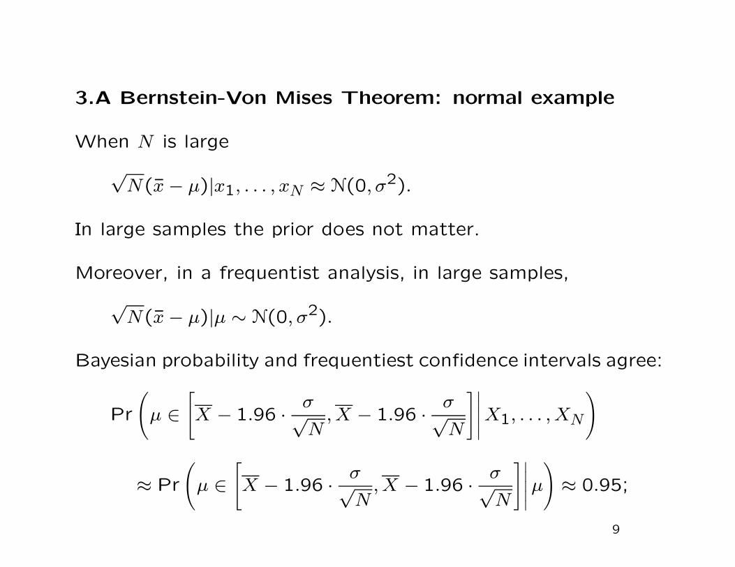
3.A Bernstein-Von Mises Theorem: normal example
When N is large
√N(x − µ)|x1, . . . , xN ≈ N(0, σ2).
In large samples the prior does not matter.
Moreover, in a frequentist analysis, in large samples,
√N(x − µ)|µ ∼ N(0, σ2).
Bayesian probability and frequentiest confidence intervals agree:
Pr
(
µ ∈[
X − 1.96 · σ√N
, X − 1.96 · σ√N
]∣
∣
∣
∣
∣
X1, . . . , XN
)
≈ Pr
(
µ ∈[
X − 1.96 · σ√N
, X − 1.96 · σ√N
]∣
∣
∣
∣
∣
µ
)
≈ 0.95;
9
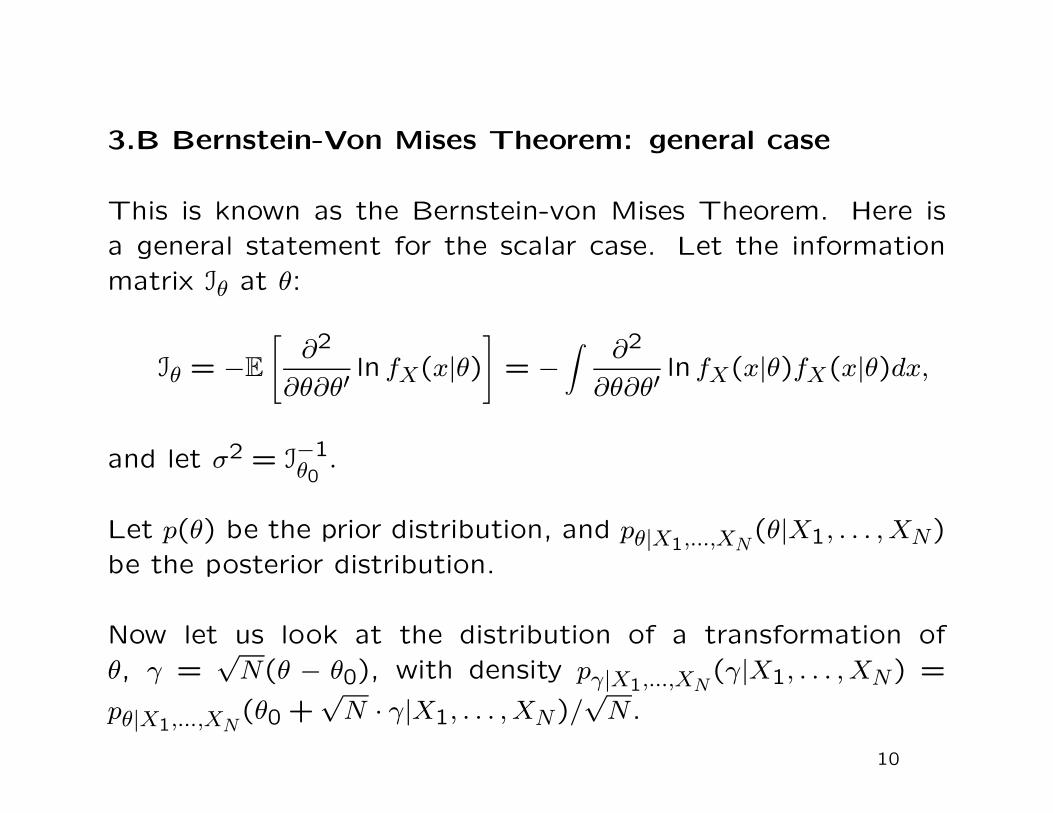
3.B Bernstein-Von Mises Theorem: general case
This is known as the Bernstein-von Mises Theorem. Here is
a general statement for the scalar case. Let the information
matrix Iθ at θ:
Iθ = −E
[
∂2
∂θ∂θ′ln fX(x|θ)
]
= −∫
∂2
∂θ∂θ′ln fX(x|θ)fX(x|θ)dx,
and let σ2 = I−1θ0
.
Let p(θ) be the prior distribution, and pθ|X1,...,XN(θ|X1, . . . , XN)
be the posterior distribution.
Now let us look at the distribution of a transformation of
θ, γ =√
N(θ − θ0), with density pγ|X1,...,XN(γ|X1, . . . , XN) =
pθ|X1,...,XN(θ0 +
√N · γ|X1, . . . , XN)/
√N .
10

Now let us look at the posterior distribution for γ if in fact the
data were generated by f(x|θ) with θ = θ0. In that case the
posterior distribution of γ converges to a normal distribution
with mean zero and variance equal to σ2 in the sense that
supγ
∣
∣
∣
∣
∣
pγ|X1,...,XN(γ|X1, . . . , XN) − 1√
2πσ2exp
(
− 1
2σ2γ2)
∣
∣
∣
∣
∣
−→ 0.
See Van der Vaart (2001), or Ferguson (1996).
11
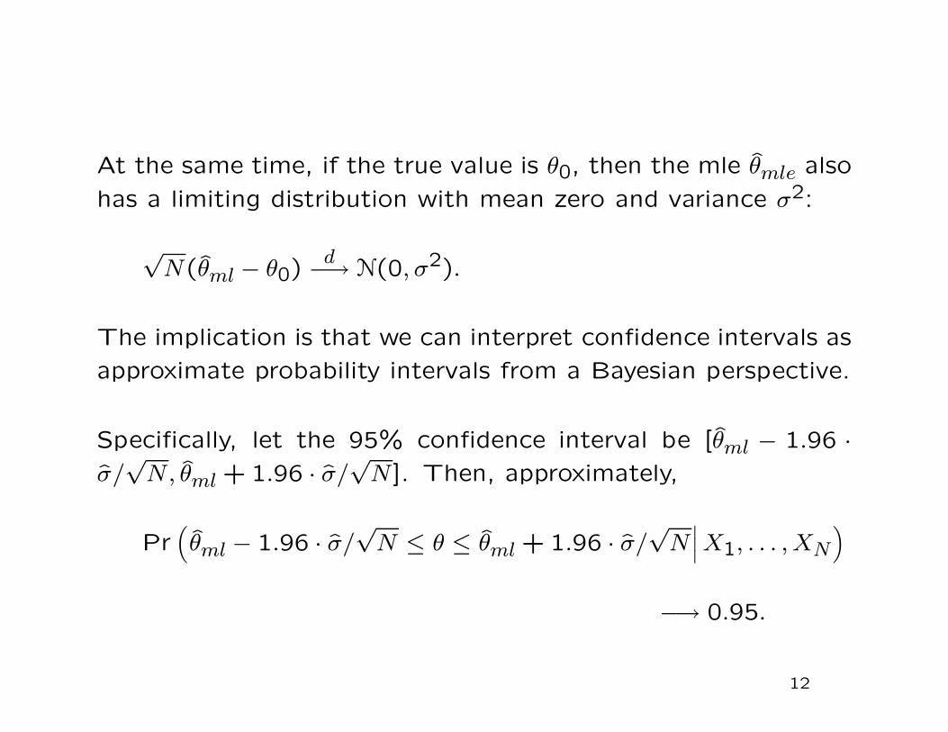
At the same time, if the true value is θ0, then the mle θmle also
has a limiting distribution with mean zero and variance σ2:
√N(θml − θ0)
d−→ N(0, σ2).
The implication is that we can interpret confidence intervals as
approximate probability intervals from a Bayesian perspective.
Specifically, let the 95% confidence interval be [θml − 1.96 ·σ/
√N, θml + 1.96 · σ/
√N]. Then, approximately,
Pr(
θml − 1.96 · σ/√
N ≤ θ ≤ θml + 1.96 · σ/√
N∣
∣
∣X1, . . . , XN
)
−→ 0.95.
12

3.C When Bernstein-Von Mises Fails
There are important cases where this result does not hold, typ-
ically when convergence to the limit distribution is not uniform.
One is the unit-root setting. In a simple first order autore-
gressive example it is still the case that with a normal prior
distribution for the autoregressive parameter the posterior dis-
tribution is normal (see Sims and Uhlig, 1991).
However, if the true value of the autoregressive parameter is
unity, the sampling distribution is not normal even in large
samples.
In such settings one has to take a more principled stand whether
one wants to make subjective probability statements, or fre-
quentist claims.
13
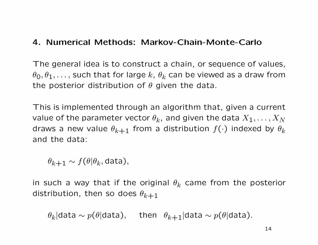
4. Numerical Methods: Markov-Chain-Monte-Carlo
The general idea is to construct a chain, or sequence of values,
θ0, θ1, . . . , such that for large k, θk can be viewed as a draw from
the posterior distribution of θ given the data.
This is implemented through an algorithm that, given a current
value of the parameter vector θk, and given the data X1, . . . , XN
draws a new value θk+1 from a distribution f(·) indexed by θk
and the data:
θk+1 ∼ f(θ|θk, data),
in such a way that if the original θk came from the posterior
distribution, then so does θk+1
θk|data ∼ p(θ|data), then θk+1|data ∼ p(θ|data).
14
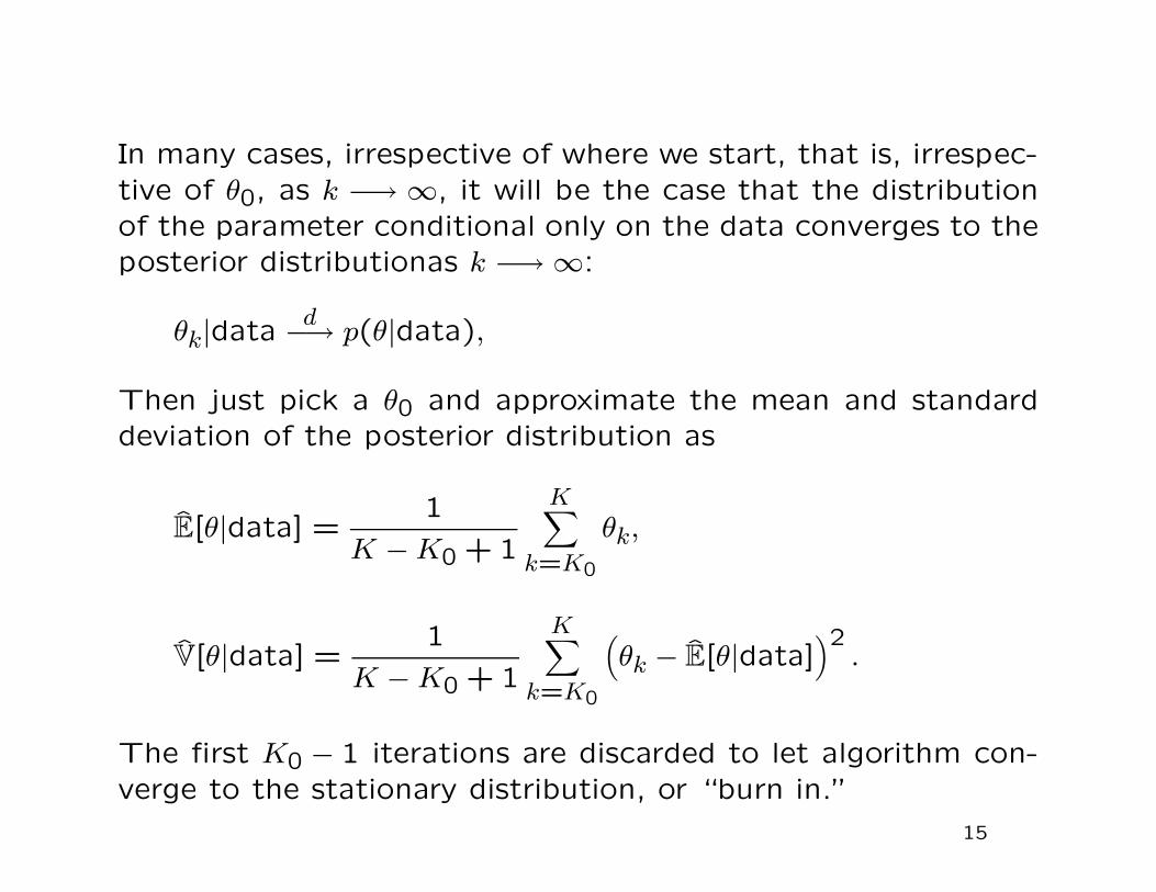
In many cases, irrespective of where we start, that is, irrespec-
tive of θ0, as k −→ ∞, it will be the case that the distribution
of the parameter conditional only on the data converges to the
posterior distributionas k −→ ∞:
θk|datad−→ p(θ|data),
Then just pick a θ0 and approximate the mean and standard
deviation of the posterior distribution as
E[θ|data] =1
K − K0 + 1
K∑
k=K0
θk,
V[θ|data] =1
K − K0 + 1
K∑
k=K0
(
θk − E[θ|data])2
.
The first K0 − 1 iterations are discarded to let algorithm con-
verge to the stationary distribution, or “burn in.”
15
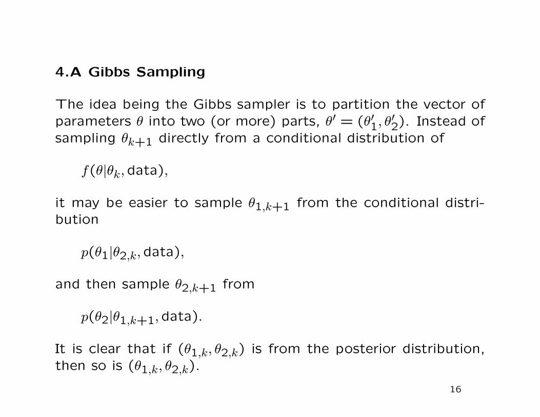
4.A Gibbs Sampling
The idea being the Gibbs sampler is to partition the vector of
parameters θ into two (or more) parts, θ′ = (θ′1, θ′2). Instead of
sampling θk+1 directly from a conditional distribution of
f(θ|θk,data),
it may be easier to sample θ1,k+1 from the conditional distri-
bution
p(θ1|θ2,k,data),
and then sample θ2,k+1 from
p(θ2|θ1,k+1,data).
It is clear that if (θ1,k, θ2,k) is from the posterior distribution,
then so is (θ1,k, θ2,k).
16
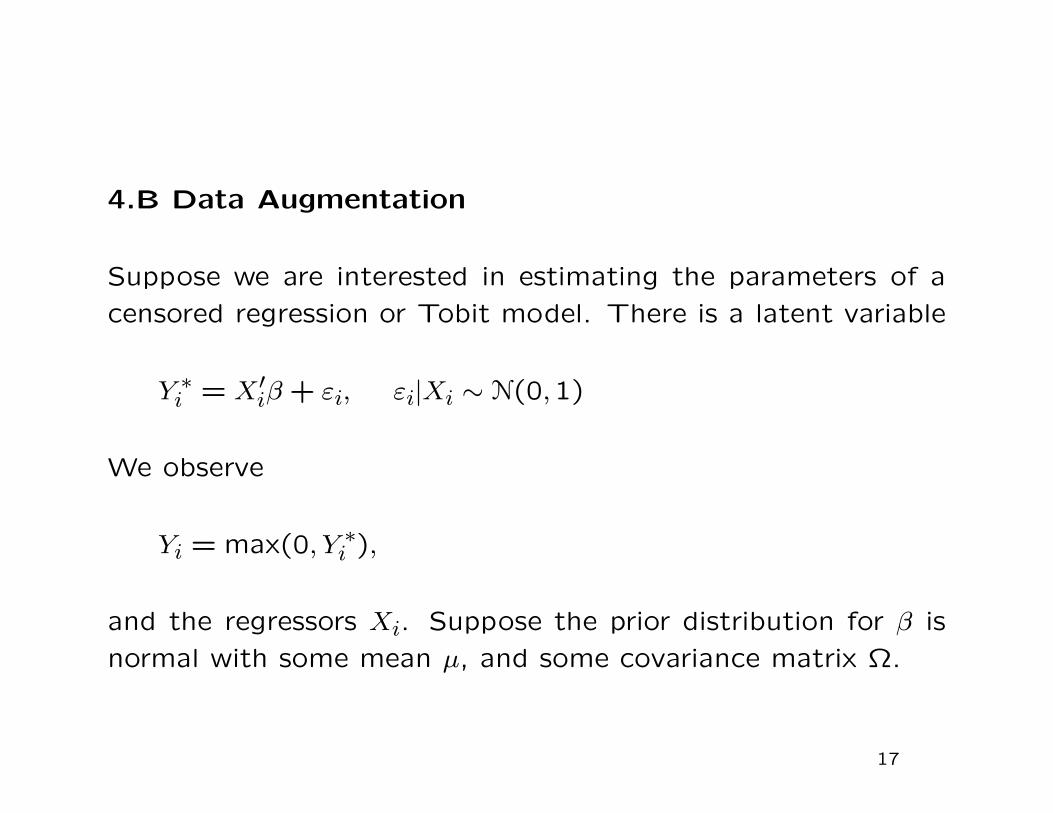
4.B Data Augmentation
Suppose we are interested in estimating the parameters of a
censored regression or Tobit model. There is a latent variable
Y ∗i = X′
iβ + εi, εi|Xi ∼ N(0,1)
We observe
Yi = max(0, Y ∗i ),
and the regressors Xi. Suppose the prior distribution for β is
normal with some mean µ, and some covariance matrix Ω.
17

The posterior distribution for β does not have a closed form
expression. The first key insight is to view both the vector
Y∗ = (Y ∗
1 , . . . , Y ∗N) and β as unknown random variables.
The Gibbs sampler consists of two steps. First we draw all the
missing elements of Y∗ given the current value of the parameter
β, say βk
Y ∗i |β, data ∼ TN
(
X′iβ, 1,0
)
,
if observation i is truncated, where TN(µ, σ2, c) denotes a trun-
cated normal distribution with mean µ, variance σ2, and trun-
cation point c (truncated from above).
Second, we draw a new value for the parameter, βk+1 given
the data and given the (partly drawn) Y∗:
p(
β|data,Y∗) ∼ N
(
(
X′X + Ω−1
)−1 ·(
X′Y + Ω−1µ
)
,(
X′X + Ω−1
)−1
18
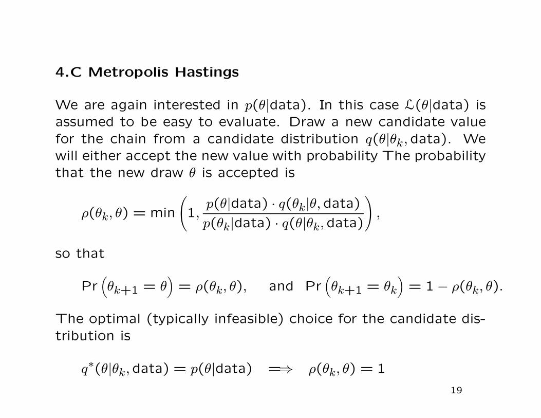
4.C Metropolis Hastings
We are again interested in p(θ|data). In this case L(θ|data) is
assumed to be easy to evaluate. Draw a new candidate value
for the chain from a candidate distribution q(θ|θk,data). We
will either accept the new value with probability The probability
that the new draw θ is accepted is
ρ(θk, θ) = min
(
1,p(θ|data) · q(θk|θ, data)
p(θk|data) · q(θ|θk,data)
)
,
so that
Pr(
θk+1 = θ)
= ρ(θk, θ), and Pr(
θk+1 = θk
)
= 1 − ρ(θk, θ).
The optimal (typically infeasible) choice for the candidate dis-
tribution is
q∗(θ|θk,data) = p(θ|data) =⇒ ρ(θk, θ) = 1
19

5. Example: Demand Models with Unobs Heterog in
Prefer.
Rossi, McCulloch, and Allenby (1996, RMA) are interested
in the optimal design of coupon policies. Supermarkets can
choose to offer identical coupons for a particular product.
Alternatively, they may choose to offer differential coupons
based on consumer’s fixed characteristics.
Taking this ever further, they could tailoring the coupon value
to the evidence for price sensitivity contained in purchase pat-
terns.
Need to allow for household-level heterogeneity in taste param-
eters and price elasticities. Even with large amounts of data
available, there will be many households for whom these pa-
rameters cannot be estimated precisely. RMA therefore use a
hieararchical, or random coefficients model.
20
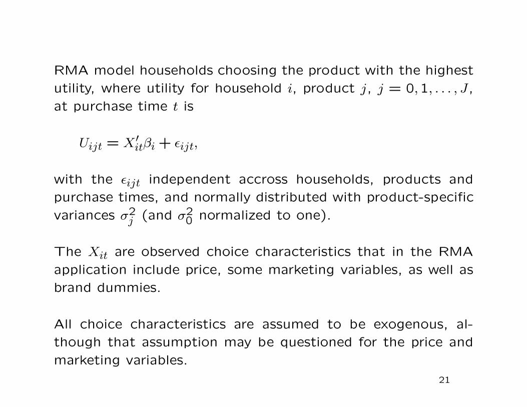
RMA model households choosing the product with the highest
utility, where utility for household i, product j, j = 0,1, . . . , J,
at purchase time t is
Uijt = X′itβi + εijt,
with the εijt independent accross households, products and
purchase times, and normally distributed with product-specific
variances σ2j (and σ2
0 normalized to one).
The Xit are observed choice characteristics that in the RMA
application include price, some marketing variables, as well as
brand dummies.
All choice characteristics are assumed to be exogenous, al-
though that assumption may be questioned for the price and
marketing variables.
21

Because for some households we have few purchases, it is not
possible to accurately estimate all βi parameters. RMA there-
fore assume that the household-specific taste parameters are
random draws from a normal distribution centered at Z′iΓ:
βi = Z′iΓ + ηi, ηi ∼ N(0,Σ).
Now Gibbs sampling can be used to obtain draws from the
posterior distribution of the βi.
22

The first step is to draw the household parameters βi given the
utilities Uijt and the common parameters Γ, Σ, and σ2j . This
is straightforward, because we have a standard normal linear
model for the utilities, with a normal prior distribution for βiwith parameters Z′
iΓ and variance Σ, and Ti observations. We
can draw from this posterior distribution for each household i.
In the second step we draw the σ2j using the results for the
normal distribution with known mean and unknown variance.
The third step is to draw from the posterior of Γ and Σ, given
the βi. This again is just a normal linear model, now with
unknown mean and unknown variance.
The fourth step is to draw the unobserved utilities given the
βi and the data. Doing this one household/choice at a time,
conditioning on the utilities for the other choices, this merely
involves drawing from a truncated normal distribution, which
is simple and fast.
23
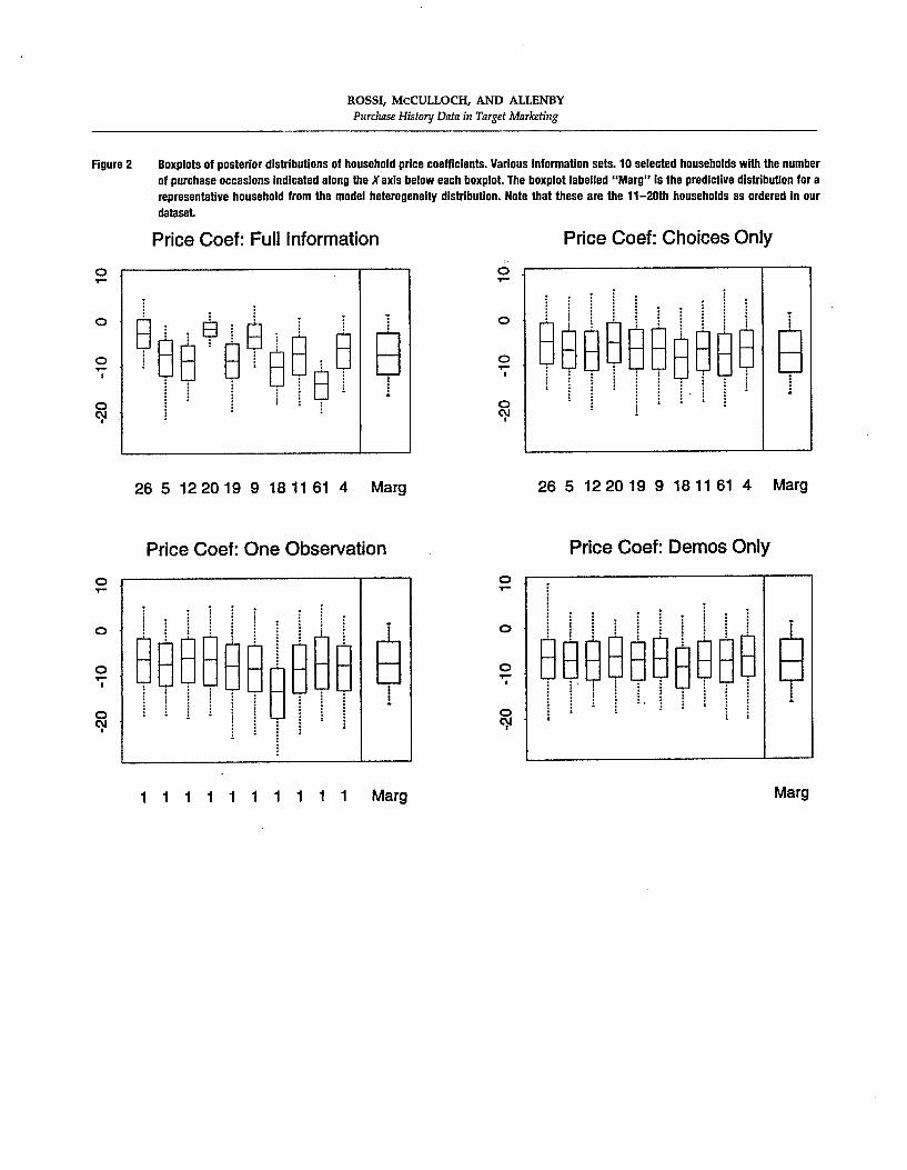
6. Example: Panel Data with Multiple Individual Specific
Param.
Chamberlain and Hirano are interested in deriving predictive
distributions for earnings using longitudinal data, using the
model
Yit = X′iβ + Vit + αi + Uit/hi.
The second component in the model, Vit, is a first order au-
toregressive component,
Vit = γ · Vit−1 + Wit,
Vi1 ∼ N(0, σ2v ), Wit ∼ N(0, σ2
w).
Uit ∼ N(0,1).
24
Analyzing this model by attempting to estimate the αi and hi
directly would be misguided. From a Bayesian perspective this
corresponds to assuming a flat prior distribution on a high-
dimensional parameter space.
To avoid such pitfalls CH model αi and hi through a random
effects specification.
αi ∼ N(0, σ2α). and hi ∼ G(m/2, τ/2).
25
In their empirical application using data from the Panel Study
of Income Dynamics (PSID), CH find strong evidence of het-
erogeneity in conditional variances.
quantiles of the predictive dist. of 1/√
hiQuantile
Sample 0.05 0.10 0.25 0.50 0.75 0.90 0.95
All (N=813) 0.04 0.05 0.07 0.11 0.20 0.45 0.81HS Dropouts (N=37) 0.06 0.08 0.11 0.16 0.27 0.49 0.79HS Grads (N=100) 0.04 0.05 0.06 0.11 0.21 0.49 0.93C Grads (N=122) 0.03 0.04 0.05 0.09 0.18 0.40 0.75
26

However, CH wish to go beyond this and infer individual-level
predictive distributions for earnings.
Taking a particular individual, one can derive the posterior dis-
tribution of αi, hi, β, σ2v , and σ2
w, given that individual’s earnings
as well as other earnings, and predict future earnings.
0.90-0.10 quantileindividual sample std 1 year out 5 years out
321 0.07 0.32 0.60
415 0.47 1.29 1.29
The variation reported in the CH results may have substantial
importance for variation in optimal savings behavior by individ-
uals.
27
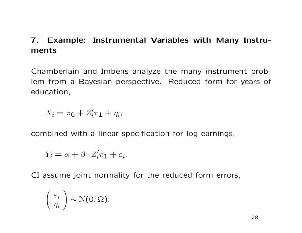
7. Example: Instrumental Variables with Many Instru-
ments
Chamberlain and Imbens analyze the many instrument prob-
lem from a Bayesian perspective. Reduced form for years of
education,
Xi = π0 + Z′iπ1 + ηi,
combined with a linear specification for log earnings,
Yi = α + β · Z′iπ1 + εi.
CI assume joint normality for the reduced form errors,
(
εiηi
)
∼ N(0,Ω).
28
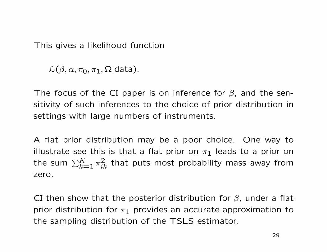
This gives a likelihood function
L(β, α, π0, π1,Ω|data).
The focus of the CI paper is on inference for β, and the sen-
sitivity of such inferences to the choice of prior distribution in
settings with large numbers of instruments.
A flat prior distribution may be a poor choice. One way to
illustrate see this is that a flat prior on π1 leads to a prior on
the sum∑K
k=1 π2ik that puts most probability mass away from
zero.
CI then show that the posterior distribution for β, under a flat
prior distribution for π1 provides an accurate approximation to
the sampling distribution of the TSLS estimator.
29

As an alternative CI suggest a hierarchical prior distribution
with
π1k ∼ N(µπ, σ2π).
In the Angrist-Krueger 1991 compulsory schooling example
there is in fact a substantive reason to believe that σ2π is small
rather than the σ2π = ∞ implicit in TSLS. If the π1k represent
the effect of the differences in the amount of required school-
ing, one would expect the magnitude of the π1k to be less than
the amount of variation in the compulsory schooling implying
the standard deviation of the first stage coefficients should not
be more than√
1/12 = 0.289.
Using the Angrist-Krueger data CI find that the posterior dis-
tribution for σπ is concentrated close to zero, with the posterior
mean and median equal to 0.119.
30
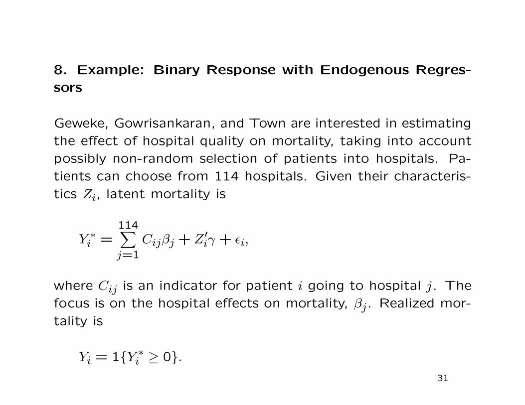
8. Example: Binary Response with Endogenous Regres-
sors
Geweke, Gowrisankaran, and Town are interested in estimating
the effect of hospital quality on mortality, taking into account
possibly non-random selection of patients into hospitals. Pa-
tients can choose from 114 hospitals. Given their characteris-
tics Zi, latent mortality is
Y ∗i =
114∑
j=1
Cijβj + Z′iγ + εi,
where Cij is an indicator for patient i going to hospital j. The
focus is on the hospital effects on mortality, βj. Realized mor-
tality is
Yi = 1Y ∗i ≥ 0.
31

The concern is about selection into the hospitals, and the pos-
sibility that this is related to unobserved components of latent
mortality GGT model latent the latent utility for patient i as-
sociated with hospital j as
C∗ij = X′
ijα + ηij,
where the Xij are hospital-individual specific characteristics,
including distance to hospital. Patient i then chooses hospital
j if
C∗ij ≥ Cik, for k = 1, . . . ,114.
32
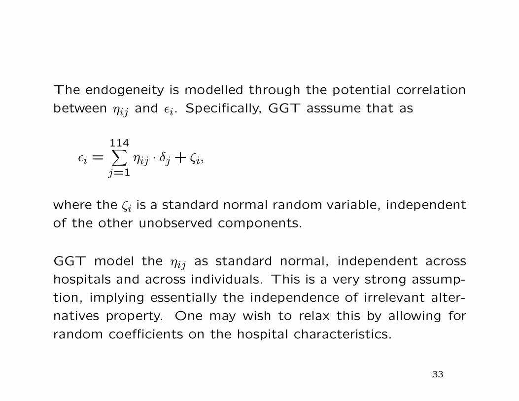
The endogeneity is modelled through the potential correlation
between ηij and εi. Specifically, GGT asssume that as
εi =114∑
j=1
ηij · δj + ζi,
where the ζi is a standard normal random variable, independent
of the other unobserved components.
GGT model the ηij as standard normal, independent across
hospitals and across individuals. This is a very strong assump-
tion, implying essentially the independence of irrelevant alter-
natives property. One may wish to relax this by allowing for
random coefficients on the hospital characteristics.
33

Given these modelling decisions GGT have a fully specified joint
distribution of hospital choice and mortality given hospital and
individual characteristics.
The log likelihood function is highly nonlinear, and it is unlikely
it can be well approximated by a quadratic function.
GGT therefore use Bayesian methods, and in particular the
Gibbs sampler to obtain draws from the posterior distribution
of interest.
In their empirical analysis GGT find strong evidence for non-
random selection. They find that higher quality hospitals at-
tract sicker patients, to the extent that a model based on
exogenous selection would have led to misleading conclusions
on hospital quality.
34

9. Example: Discrete Choice Models with Unobserved
Choice Characteristics
Athey and Imbens (2007, AI) study discrete choice models,
allowing both for unobserved individual heterogeneity in taste
parameters as well as for multiple unobserved choice charac-
teristics.
In such settings the likelihood function is multi-modal, and
frequentist approximations based on quadratic approximations
to the log likelihood function around the maximum likelihood
estimator are unlikely to be accurate.
35
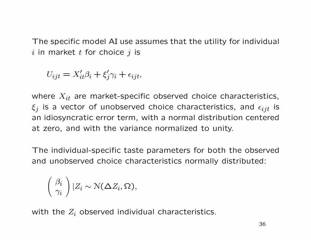
The specific model AI use assumes that the utility for individual
i in market t for choice j is
Uijt = X′itβi + ξ′jγi + εijt,
where Xit are market-specific observed choice characteristics,
ξj is a vector of unobserved choice characteristics, and εijt is
an idiosyncratic error term, with a normal distribution centered
at zero, and with the variance normalized to unity.
The individual-specific taste parameters for both the observed
and unobserved choice characteristics normally distributed:
(
βiγi
)
|Zi ∼ N(∆Zi,Ω),
with the Zi observed individual characteristics.
36
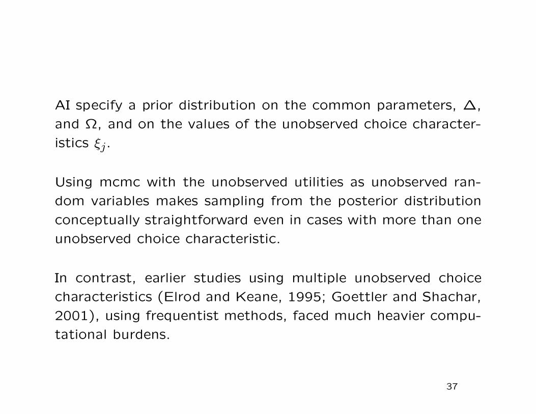
AI specify a prior distribution on the common parameters, ∆,
and Ω, and on the values of the unobserved choice character-
istics ξj.
Using mcmc with the unobserved utilities as unobserved ran-
dom variables makes sampling from the posterior distribution
conceptually straightforward even in cases with more than one
unobserved choice characteristic.
In contrast, earlier studies using multiple unobserved choice
characteristics (Elrod and Keane, 1995; Goettler and Shachar,
2001), using frequentist methods, faced much heavier compu-
tational burdens.
37

Econometrics of Cross Section and Panel DataLecture 14: Control Functions
Jeff WooldridgeMichigan State University
cemmap/PEPA, June 2014
1. Introduction2. Linear Models: IV versus Control Functions3. Correlated Random Coefficient Models4. Nonlinear Models5. Panel Data
1

1. Introduction∙ The term “control function” has been used in differentways.∙ A control function is a variable added to a model thatrenders an endogenous explanatory variable (EEV)exogenous.∙ A “proxy variable” can be viewed as a CF.∙ Focus here is on CFs contructed under instrumentalvariables assumptions.
2

2. Linear Models: IV versus Control Functions∙Models linear in parameters are usually estimated by twostage least squares (2SLS).∙ The control function (CF) approach relies on similaridentification conditions.∙ In models with random coefficients or nonlinearities, theCF approach identifies causal quantities of interest – at thecost of more assumptions.
3
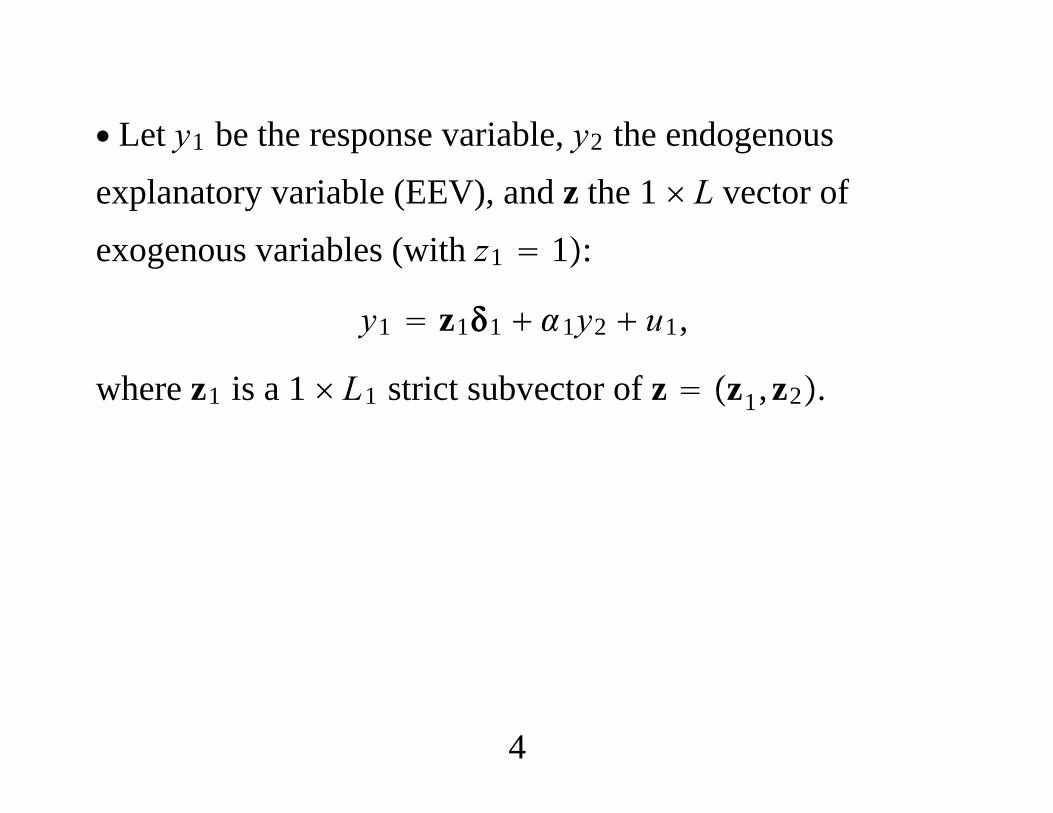
∙ Let y1 be the response variable, y2 the endogenousexplanatory variable (EEV), and z the 1 L vector ofexogenous variables (with z1 1:
y1 z11 1y2 u1,
where z1 is a 1 L1 strict subvector of z z1,z2.
4

∙ Consider the (weakest) exogeneity assumption
Ez′u1 0.
∙ Reduced form for y2:
y2 z2 v2
Ez′v2 0 (definitional)
where 2 is L 1.
5
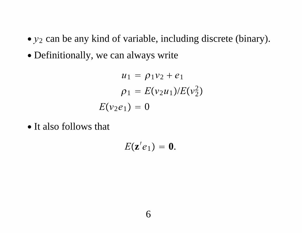
∙ y2 can be any kind of variable, including discrete (binary).∙ Definitionally, we can always write
u1 1v2 e1
1 Ev2u1/Ev22
Ev2e1 0
∙ It also follows that
Ez′e1 0.
6
∙ Plug u1 1v2 e1 into y1 z11 1y2 u1:
y1 z11 1y2 1v2 e1,
where v2 is an explanatory variable in the equation.∙ The new error, e1, is uncorrelated with y2 as well as withv2 and z.∙ v2 is the control function.
7
∙ Two-step procedure:1. Regress yi2 on zi1, zi2 and obtain the reduced formresiduals, vi2.2. Regress
yi1 on zi1, yi2, and vi2.
∙ These OLS estimates are control function estimates.
8
∙ Algebra: The control function estimates of 1 and 1 areidentical to the 2SLS estimates of
yi1 zi11 1yi2 ui1
using zi zi1,zi2 as instruments.∙What does the CF approach buy us in this case?
A simple, heteroskedasticity-robust test forendogeneity of y2: Use the t statistic on vi2.
9
∙Many CF approaches are based on Ey1|z,y2 rather thanlinear projections.∙ Then the estimating equation is obtained from
Ey1|z,y2 z11 1y2 Eu1|z,y2.
We need substantive restrictions to obtain the controlfunction, Eu1|z,y2.
Identification still requires that Eu1|z,y2 dependson z2.
10

∙ Suppose y2 is binary:
y1 z11 1y2 u1
y2 1z2 e2 ≥ 0u1,e2 is independent of z
Eu1|e2 1e2
e2 Normal0,1
∙ It can be show that
Eu1|z,y2 1y2z2 − 1 − y2−z2,
where / is the inverse Mills ratio (IMR).
11

∙ Heckman two-step approach (for endogeneity, not sampleselection):
1. Probit of yi2 on zi to get 2 and compute the generalizedresiduals:
gri2 ≡ yi2zi2 − 1 − yi2−zi2
2. Regress yi1 on zi1, yi2, gri2, i 1, . . . ,N.
∙ The t statistic on gri2 is a valid test of
H0 : 1 0.
12
∙When 1 ≠ 0, consistency of the Heckman CF estimator
hinges on the model for Dy2|z being correctly specified(and other assumptions).∙ If we just apply 2SLS directly to
y1 z11 1y2 u1
using IVs z, it does not matter if y2 is continuous, discrete,or some mixture: 2SLS is consistent and asymptoticallynormal.
13
∙ If the linear model is incorrect – for example, we neglectheterogeneity – the 2SLS and Heckman estimates can bevery different.∙ As an alternative to regular 2SLS, can use the probit fitted
values, zi2, as instrument for y2. Does not require probit model to be correct but does
require Eu1|z 0.
14
3. Correlated Random Coefficient Models∙With CF methods can learn about nature of theheterogeneous effects.∙Modify the original equation as
y1 1 z11 a1y2 u1,
where a1, the “random coefficient” on y2. 1 Ea1 is the average partial effect or population
average effect.
15
∙ For a random draw i:
yi1 1 zi11 ai1yi2 ui1
∙Write a1 1 v1 where Ev1 0.∙ Rewrite the equation as
y1 1 z11 1y2 u1 v1y2
16
∙ General problem with applying IV: The error termu1 v1y2 is not necessarily uncorrelated with theinstruments z, even under
Eu1|z Ev1|z 0.
∙When will 2SLS consistently estimate 1,1 whenai1 ≠ 1? A sufficient condition that allows for anyunconditional correlation is
Covv1,y2|z Covv1,y2.
17
∙ The CF approach due to Garen (1984) is based on
y2 z2 v2
Ey1|z,v2 1 z11 1y2 Eu1|z,v2 Ev1|z,v2y2
1 z11 1y2 1v2 1v2y2
∙ CF estimator:
yi1 on 1, zi1, yi2, vi2, vi2yi2,
where vi2 are the reduced form residuals.
18
∙ Taking the Imbens and Angrist (1994) view, IV onlyestimates a local average treatment effect (LATE).∙ The CF approach (potentially) identifies more. In theGaren setup,
Eai1|zi,vi2 Eai1|vi2 1 1vi2,
which is estimated for unit i as 1 1vi2. Can average across subgroups in the population.
19
∙ In the case of binary y2, we have the “endogenousswitching regression” model.∙ Under standard assumptions,
Ey1|z,y2 1 z11 1y2
1 ge2y2,z2 1 ge2y2,z2 y2,
where
ge2y2,z2 y2z2 − 1 − y2−z2
∙ Allow all coefficients to differ across regime.
20
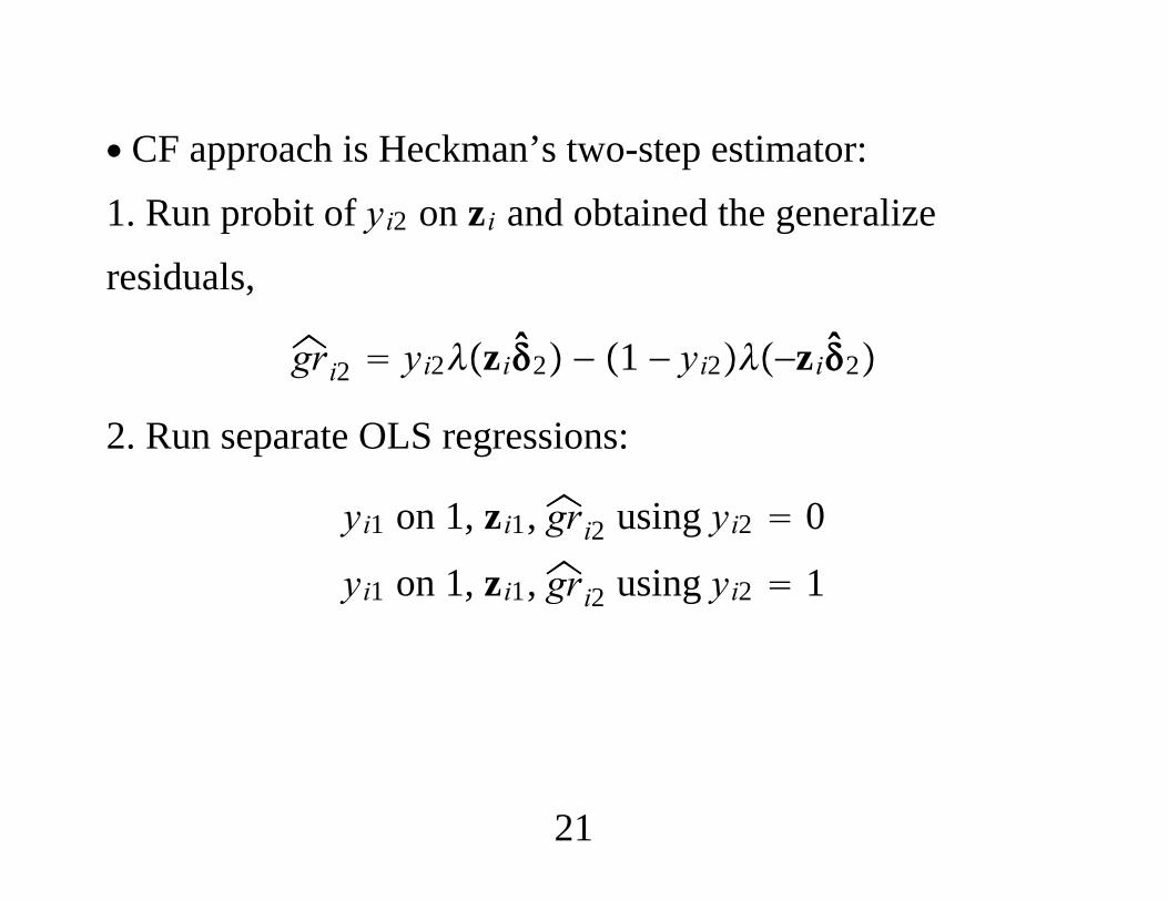
∙ CF approach is Heckman’s two-step estimator:1. Run probit of yi2 on zi and obtained the generalizeresiduals,
gri2 yi2zi2 − 1 − yi2−zi2
2. Run separate OLS regressions:
yi1 on 1, zi1, gri2 using yi2 0
yi1 on 1, zi1, gri2 using yi2 1
21
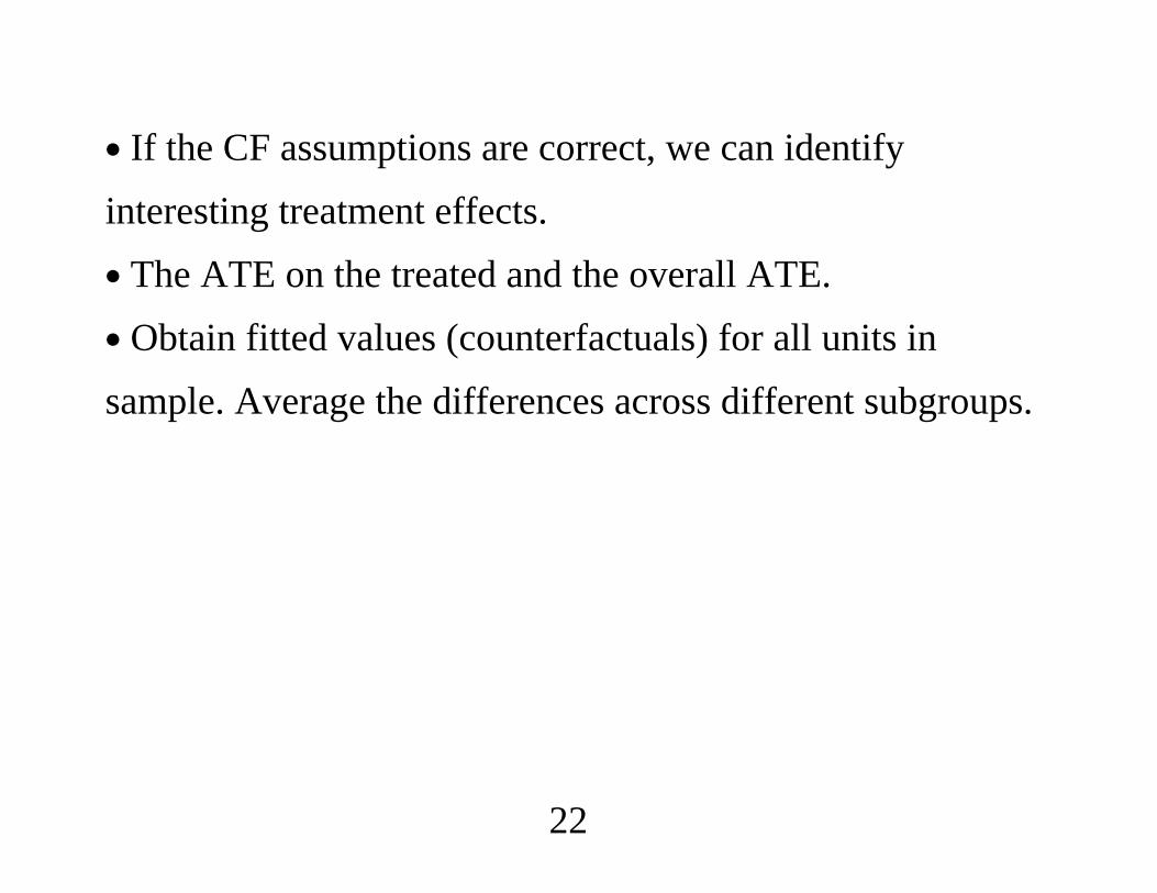
∙ If the CF assumptions are correct, we can identifyinteresting treatment effects.∙ The ATE on the treated and the overall ATE.∙ Obtain fitted values (counterfactuals) for all units insample. Average the differences across different subgroups.
22

∙ Example: Estimating the causal effect of attending aCatholic high school in the United States.∙ Data a subset of Altonji, Elder, and Tabor (2005, Journalof Human Resources). 7,444 students. About 6% attended aCatholic high school.
23

∙ Simple Model: Control for parents’ education and familyincome [logincome].∙ Outcome is score on a 12th grade math test, math12.∙ Treatment is binary: Attending a Catholic high school,cathhs. Instrument is distance to nearest Catholic highschool (in bins).
24
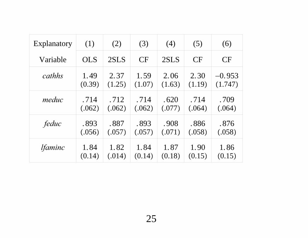
Explanatory (1) (2) (3) (4) (5) (6)
Variable OLS 2SLS CF 2SLS CF CF
cathhs0.391.49
1.252.37
1.071.59
1.632.06
1.192.30
1.747−0.953
meduc.062. 714
.062. 712
.062. 714
.077. 620
.064. 714
.064. 709
feduc.056. 893
.057. 887
.057. 893
.071. 908
.058. 886
.058. 876
lfaminc0.141.84
.0141.82
0.141.84
0.181.87
0.151.90
0.151.86
25

(1) (2) (3) (4) (5) (6)
cathhs meduc −meduc − − −0.731.61
.262−. 077
.262−. 085
cathhs feduc −feduc − − −0.684−. 198
0.235. 089
0.238. 184
cathhs lfaminc −lfaminc − − −2.082−. 688
0.61−1.10
0.634−. 691
gen_resid − −.594−. 061 −
.632−. 290
0.80−1.52
cathhs gen_resid − − − − −1.313.31
Observations 7,444 7,444 7,444 7,444 7,444 7,444
26

∙ ATT 3.99; ATU −1.27; ATE −. 95∙ One can go further. Allow coefficients on exogenousvariables to be heterogeneous.∙ Then, the generalized residual gets interacted witheverything in the table.∙ See Wooldridge (JHR, forthcoming).
27
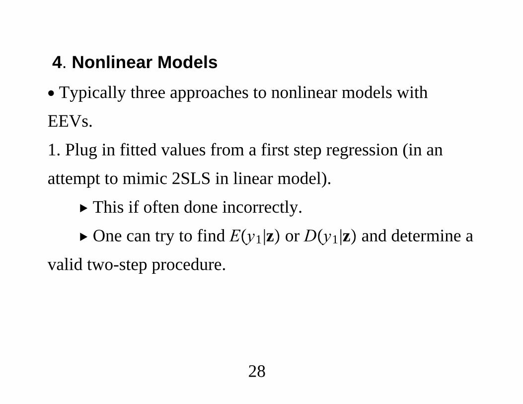
4. Nonlinear Models∙ Typically three approaches to nonlinear models withEEVs.1. Plug in fitted values from a first step regression (in anattempt to mimic 2SLS in linear model).
This if often done incorrectly. One can try to find Ey1|z or Dy1|z and determine a
valid two-step procedure.
28
2. CF approach: Plug in residuals obtained in a first stageinto the second-stage problem.
Can be made very flexible, even nonparametric insome cases.3. Maximum Likelihood (often limited information): Usemodels for Dy1|y2,z and Dy2|z jointly.
29
Binary and Fractional Responses∙ Probit model:
y1 1z11 1y2 u1 ≥ 0,
where u1|z Normal0,1. Analysis goes through if wereplace z1,y2 with any known function x1 ≡ g1z1,y2.
30
∙ The Rivers-Vuong (1988) approach is to make ahomoskedastic-normal assumption on the reduced form fory2,
y2 z2 v2, v2|z Normal0,22.
∙ Under normality, can show
Py1 1|z,y2 z11 1y2 1v2
where 1 Corru1,v2 and each coefficient is multiplied
by 1 − 12−1/2.
31
The Rivers-Vuong CF approach:(i) OLS of yi2 on zi, to obtain the residuals, vi2.(ii) Probit of yi1 on zi1, yi2, vi2 to estimate the scaled
coefficients. A simple t test on v2 is valid to testH0 : 1 0.
32
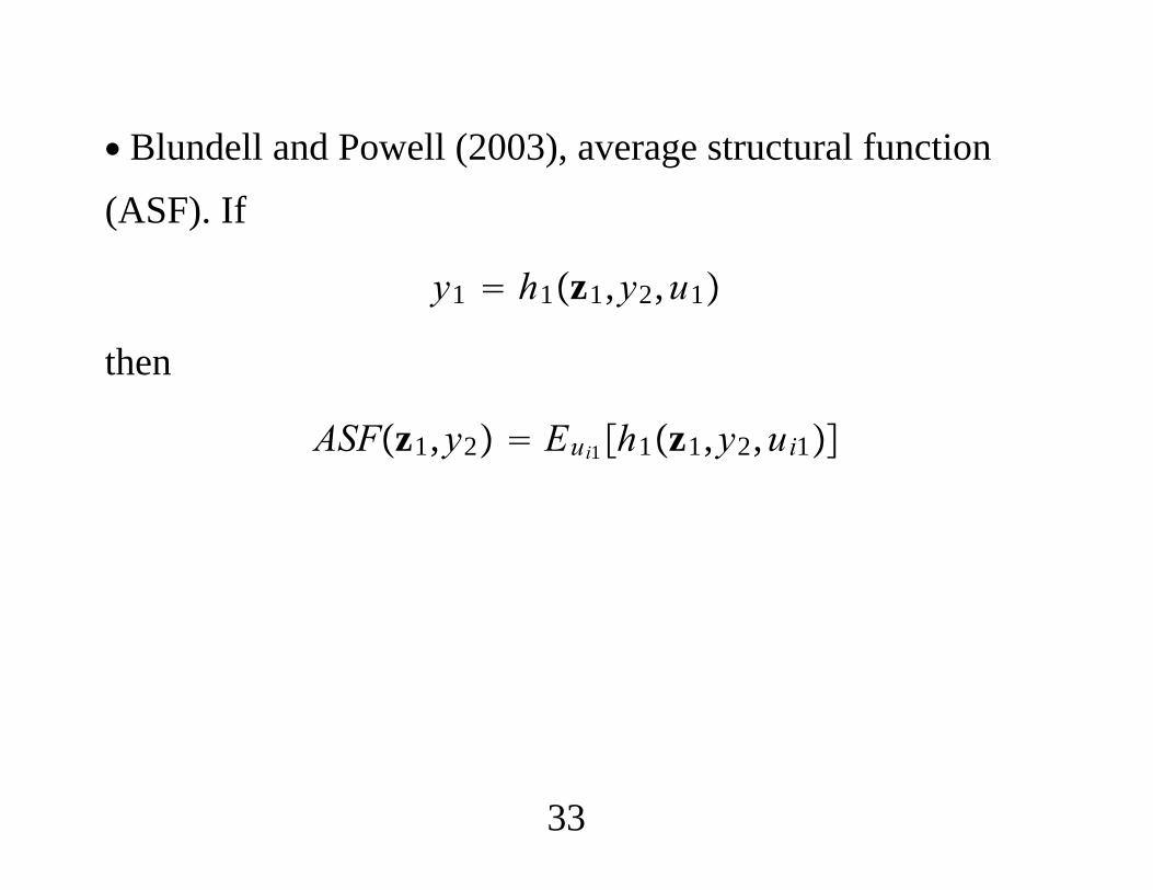
∙ Blundell and Powell (2003), average structural function(ASF). If
y1 h1z1,y2,u1
then
ASFz1,y2 Eui1h1z1,y2,ui1
33
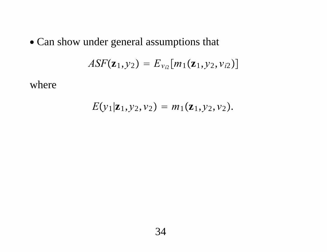
∙ Can show under general assumptions that
ASFz1,y2 Evi2m1z1,y2,vi2
where
Ey1|z1,y2,v2 m1z1,y2,v2.
34
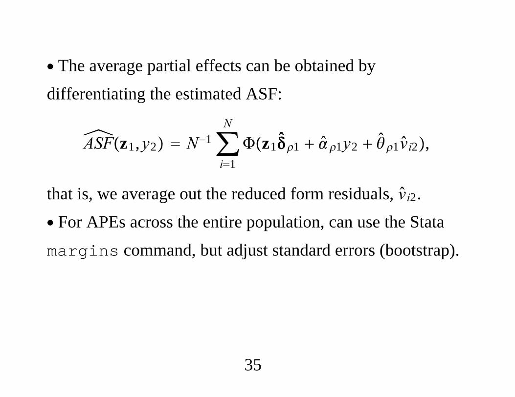
∙ The average partial effects can be obtained bydifferentiating the estimated ASF:
ASFz1,y2 N−1∑i1
N
z11 1y2 1vi2,
that is, we average out the reduced form residuals, vi2.∙ For APEs across the entire population, can use the Statamargins command, but adjust standard errors (bootstrap).
35
∙ CF has advantages over the “plug-in approach”:1. OLS on the reduced form, and get fitted values,
ŷi2 zi2.2. Probit of yi1 on zi1,ŷi2.∙ Drawbacks to plug-in approach:a. Harder to estimate APEs and test for endogeneity.b. One might be tempted to plug ŷ2 into nonlinear functions,say y2
2 or y2z1. This does not result in consistent estimation
of the scaled parameters or the partial effects.
36
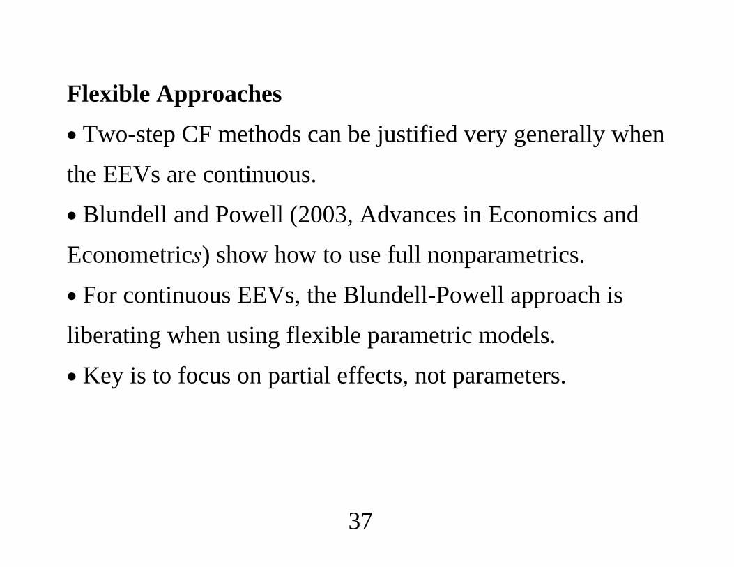
Flexible Approaches∙ Two-step CF methods can be justified very generally whenthe EEVs are continuous.∙ Blundell and Powell (2003, Advances in Economics andEconometrics) show how to use full nonparametrics.∙ For continuous EEVs, the Blundell-Powell approach isliberating when using flexible parametric models.∙ Key is to focus on partial effects, not parameters.
37

∙ Example: Suppose y1 is a binary or fractional variable andy2 is continuous.∙ Let
yi2 h2zi vi2
where vi2 is independent of zi.∙ Skip over the “structural” model for y1 and specify
Eyi1|yi2,zi1,vi2 ≈ xi11 vi2 xi11 1vi22
38
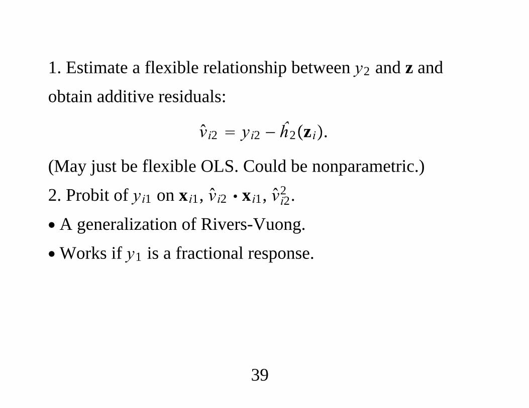
1. Estimate a flexible relationship between y2 and z andobtain additive residuals:
vi2 yi2 − ĥ2zi.
(May just be flexible OLS. Could be nonparametric.)2. Probit of yi1 on xi1, vi2 xi1, vi22 .
∙ A generalization of Rivers-Vuong.∙Works if y1 is a fractional response.
39
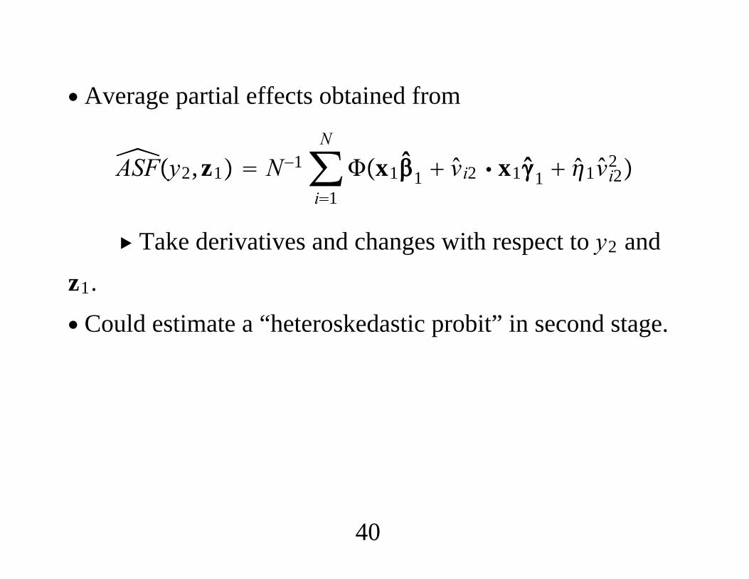
∙ Average partial effects obtained from
ASFy2,z1 N−1∑i1
N
x11 vi2 x11 1vi22
Take derivatives and changes with respect to y2 andz1.∙ Could estimate a “heteroskedastic probit” in second stage.
40

Example: Married Women’s Labor Force Participation∙ Other sources of income, nwifeinc (in $1,000s) is treated asendogenous.∙ Instrument is husband’s education.∙ Data from 1991 CPS.
41
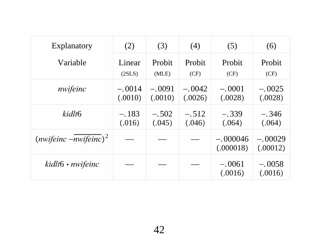
Explanatory (2) (3) (4) (5) (6)
Variable(2SLS)
Linear(MLE)
Probit(CF)
Probit(CF)
Probit(CF)
Probit
nwifeinc.0010−. 0014
.0010−. 0091
.0026−. 0042
.0028−. 0001
.0028−. 0025
kidlt6.016−. 183
.045−. 502
.046−. 512
.064−. 339
.064−. 346
nwifeinc −nwifeinc2 — — —.000018−. 000046
.00012−. 00029
kidlt6 nwifeinc — — —.0016−. 0061
.0016−. 0058
42
v2 — —.0027−. 0052
.0027−. 0055
.0072−. 0273
v22 — — — —
.00013−. 00052
v2nwifeinc — — — —.00024. 00075
APEnwifeinc.0010−. 0014
.0002−. 0033
.0009−. 0015
.00010−. 00097
.0010−. 0015
Observations 5,634 5,634 5,634 5,634 5,634
43
Average partial effects of nwifeinc at different quartiles.
(4) (5) (6)No Young Children
(CF)Probit
(CF)Probit
(CF)Probit
25th percentile.00087−. 00143
.00105. 00026
.00129. 00163
50th percentile.00091−. 00146
.00098−. 00014
.00095−. 00068
75th percentile.00095−. 00149
.00096−. 00065
.00158−. 00367
44
≥ 1 Young Child (4) (5) (6)25th percentile
.00099−. 00157
.00120−. 00197
.00129−. 00067
50th percentile.00099−. 00156
.00115−. 00240
.00098−. 00295
75th percentile.00097−. 00155
.00109−. 00291
.00124−. 00535
45
Discrete EEVs∙ Suppose y1 and y2 are binary, and the “bivariate probit”model holds:
y1 1z11 1y2 u1 0y2 1z2 e2 0
where u1,e2 is independent of z and
u1
e2 Normal
00
,1 1
1 1
46

∙ As show in Wooldridge (2013, forthcoming, J of E), avariable addition version of the score test is simple:(i) Probit of yi2 on zi to obtain the generalized residuals,
gri2.
(ii) Probit of yi1 on zi1, yi2, gri2 and use usual t statistic on
gri2.
∙ Suggestion: Use (ii) as a correction for endogeneity, notjust a test.
47
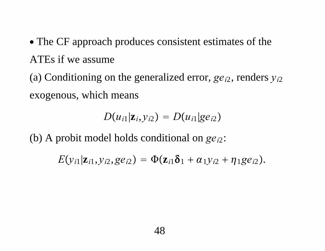
∙ The CF approach produces consistent estimates of theATEs if we assume(a) Conditioning on the generalized error, gei2, renders yi2exogenous, which means
Dui1|zi,yi2 Dui1|gei2
(b) A probit model holds conditional on gei2:
Eyi1|zi1,yi2,gei2 zi11 1yi2 1gei2.
48
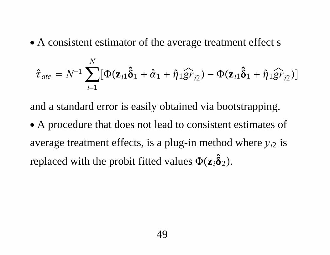
∙ A consistent estimator of the average treatment effect s
ate N−1∑i1
N
zi11 1 1gri2 − zi11 1gri2
and a standard error is easily obtained via bootstrapping.∙ A procedure that does not lead to consistent estimates ofaverage treatment effects, is a plug-in method where yi2 is
replaced with the probit fitted values zi2.
49
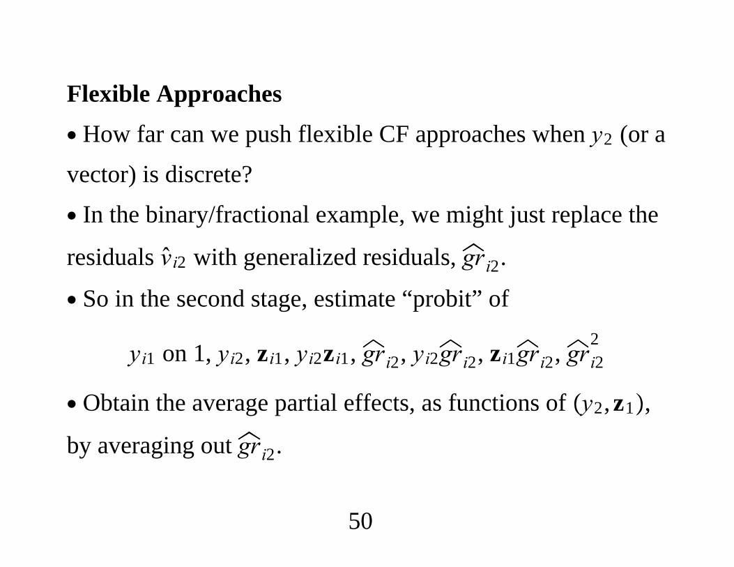
Flexible Approaches∙ How far can we push flexible CF approaches when y2 (or avector) is discrete?∙ In the binary/fractional example, we might just replace the
residuals vi2 with generalized residuals, gri2.
∙ So in the second stage, estimate “probit” of
yi1 on 1, yi2, zi1, yi2zi1, gri2, yi2gri2, zi1gri2, gri22
∙ Obtain the average partial effects, as functions of y2,z1,
by averaging out gri2.
50
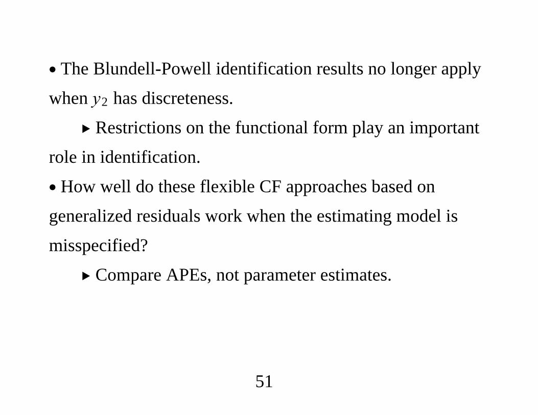
∙ The Blundell-Powell identification results no longer applywhen y2 has discreteness.
Restrictions on the functional form play an importantrole in identification.∙ How well do these flexible CF approaches based ongeneralized residuals work when the estimating model ismisspecified?
Compare APEs, not parameter estimates.
51
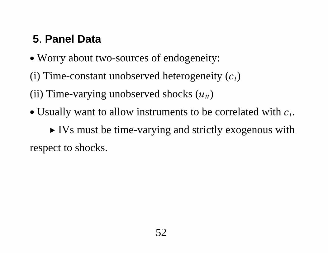
5. Panel Data∙Worry about two-sources of endogeneity:(i) Time-constant unobserved heterogeneity (ci)(ii) Time-varying unobserved shocks (uit)∙ Usually want to allow instruments to be correlated with ci.
IVs must be time-varying and strictly exogenous withrespect to shocks.
52
∙ Can combine the Chamberlain-Mundlak approach tocorrelated random effects (CRE) models with controlfunction approaches for traditional endogeneity.
Papke and Wooldridge (2008, Journal ofEconometrics) is an example.
53

"Econometrics of Cross Section and Panel Data"
Lecture 15
Weak and Many Instruments
Guido Imbens
Cemmap Lectures, UCL, June 2014
1. Introduction
Standard normal asymptotic approximation to sampling distri-
bution of IV, TSLS, and LIML estimators relies on non-zero
correlation between instruments and endogenous regressors.
If correlation is close to zero, these approximations are not
accurate even in fairly large samples.
In the just identified case TSLS/LIML confidence intervals will
still be fairly wide in most cases, even if not valid, unless degree
of endogeneity is very high. If concerned with this, alternative
confidence intervals are available that are valid uniformly. No
better estimators available.
2
In the case with large degree of overidentification TSLS has
poor properties: considerable bias towards OLS, and substan-
tial underestimation of standard errors.
LIML is much better in terms of bias, but its standard error is
not correct. A simple multiplicative adjustment to conventional
LIML standard errors based on Bekker asymptotics or random
effects likelihood works well.
Overall: use LIML, with Bekker-adjusted standard errors.
(as long as instruments are valid, see Kolesar et al)
3
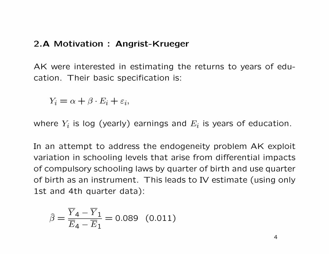
2.A Motivation : Angrist-Krueger
AK were interested in estimating the returns to years of edu-
cation. Their basic specification is:
Yi = α + β · Ei + εi,
where Yi is log (yearly) earnings and Ei is years of education.
In an attempt to address the endogeneity problem AK exploit
variation in schooling levels that arise from differential impacts
of compulsory schooling laws by quarter of birth and use quarter
of birth as an instrument. This leads to IV estimate (using only
1st and 4th quarter data):
β =Y 4 − Y 1
E4 − E1= 0.089 (0.011)
4

2.B AK with Many Instruments
AK also present estimates based on additional instruments.
They take the basic 3 qob dummies and interact them with 50
state and 9 year of birth dummies.
Here (following Chamberlain and Imbens) we interact the single
binary instrument with state times year of birth dummies to get
500 instruments. Also including the state times year of birth
dummies as exogenous covariates leads to the following model:
Yi = X′iβ + εi, E[Zi · εi] = 0,
where Xi is the 501-dimensional vector with the 500 state/year
dummies and years of education, and Zi is the vector with 500
state/year dummies and the 500 state/year dummies multiply-
ing the indicator for the fourth quarter of birth.
5
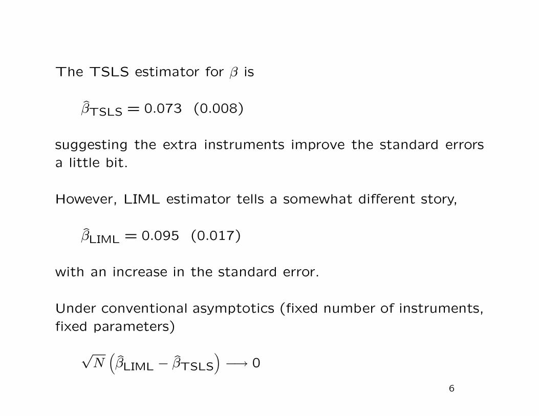
The TSLS estimator for β is
βTSLS = 0.073 (0.008)
suggesting the extra instruments improve the standard errors
a little bit.
However, LIML estimator tells a somewhat different story,
βLIML = 0.095 (0.017)
with an increase in the standard error.
Under conventional asymptotics (fixed number of instruments,
fixed parameters)
√N(βLIML − βTSLS
)−→ 0
6
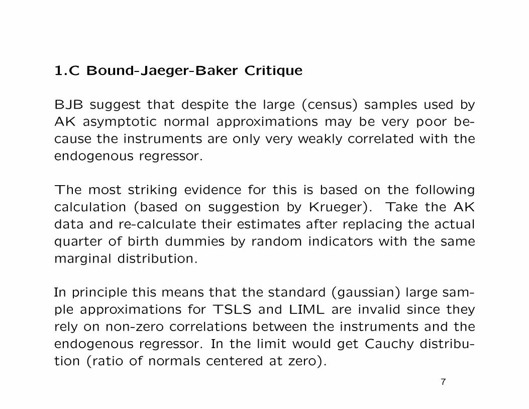
1.C Bound-Jaeger-Baker Critique
BJB suggest that despite the large (census) samples used by
AK asymptotic normal approximations may be very poor be-
cause the instruments are only very weakly correlated with the
endogenous regressor.
The most striking evidence for this is based on the following
calculation (based on suggestion by Krueger). Take the AK
data and re-calculate their estimates after replacing the actual
quarter of birth dummies by random indicators with the same
marginal distribution.
In principle this means that the standard (gaussian) large sam-
ple approximations for TSLS and LIML are invalid since they
rely on non-zero correlations between the instruments and the
endogenous regressor. In the limit would get Cauchy distribu-
tion (ratio of normals centered at zero).
7
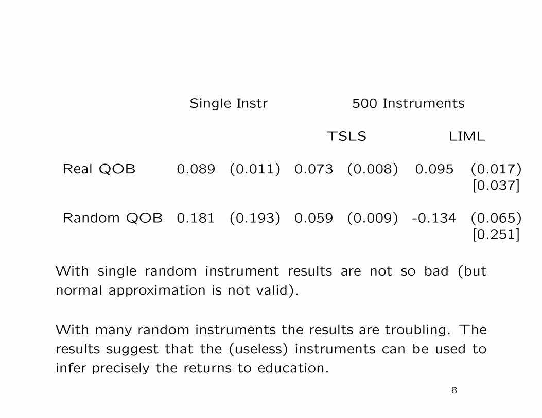
Single Instr 500 Instruments
TSLS LIML
Real QOB 0.089 (0.011) 0.073 (0.008) 0.095 (0.017)[0.037]
Random QOB 0.181 (0.193) 0.059 (0.009) -0.134 (0.065)[0.251]
With single random instrument results are not so bad (but
normal approximation is not valid).
With many random instruments the results are troubling. The
results suggest that the (useless) instruments can be used to
infer precisely the returns to education.
8
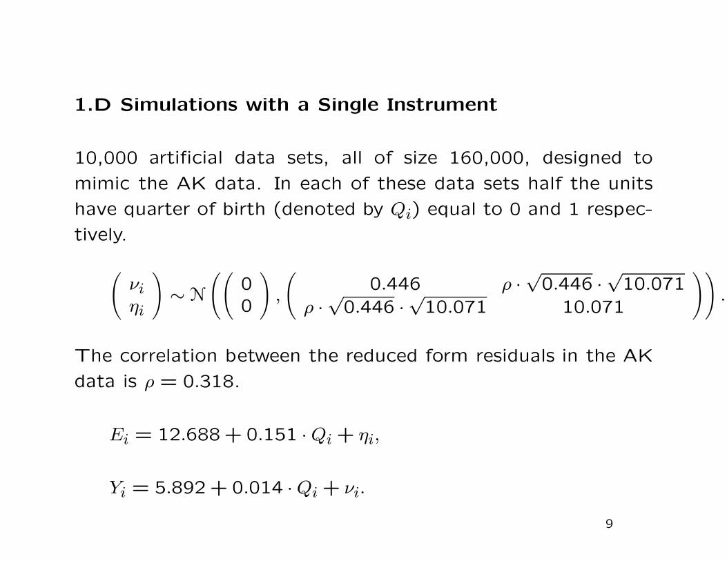
1.D Simulations with a Single Instrument
10,000 artificial data sets, all of size 160,000, designed to
mimic the AK data. In each of these data sets half the units
have quarter of birth (denoted by Qi) equal to 0 and 1 respec-
tively.
(νiηi
)∼ N
((00
),
(0.446 ρ ·
√0.446 ·
√10.071
ρ ·√
0.446 ·√
10.071 10.071
)).
The correlation between the reduced form residuals in the AK
data is ρ = 0.318.
Ei = 12.688 + 0.151 · Qi + ηi,
Yi = 5.892 + 0.014 · Qi + νi.
9

Now we calculate the IV estimator and its standard error, using
either the actual qob variable or a random qob variable as the
instrument.
We are interested in the size of tests of the null that coefficient
on years of education is equal to 0.089 = 0.014/0.151.
We base the test on the t-statistic. Thus we reject the null if
the ratio of the point estimate minus 0.089 and the standard
error is greater than 1.96 in absolute value.
We repeat this for 12 different values of the reduced form
error correlation. In Table 3 we report the coverage rate and
the median and 0.10 quantile of the width of the estimated
95% confidence intervals.
10
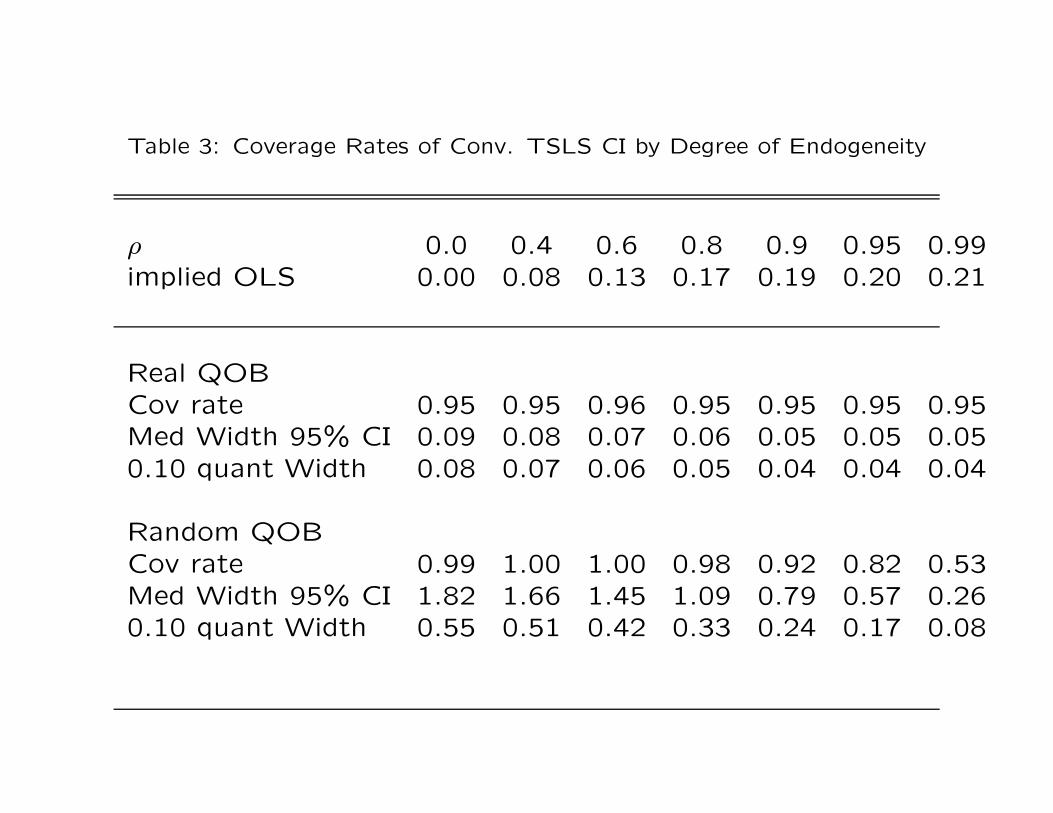
Table 3: Coverage Rates of Conv. TSLS CI by Degree of Endogeneity
ρ 0.0 0.4 0.6 0.8 0.9 0.95 0.99implied OLS 0.00 0.08 0.13 0.17 0.19 0.20 0.21
Real QOBCov rate 0.95 0.95 0.96 0.95 0.95 0.95 0.95Med Width 95% CI 0.09 0.08 0.07 0.06 0.05 0.05 0.050.10 quant Width 0.08 0.07 0.06 0.05 0.04 0.04 0.04
Random QOBCov rate 0.99 1.00 1.00 0.98 0.92 0.82 0.53Med Width 95% CI 1.82 1.66 1.45 1.09 0.79 0.57 0.260.10 quant Width 0.55 0.51 0.42 0.33 0.24 0.17 0.08
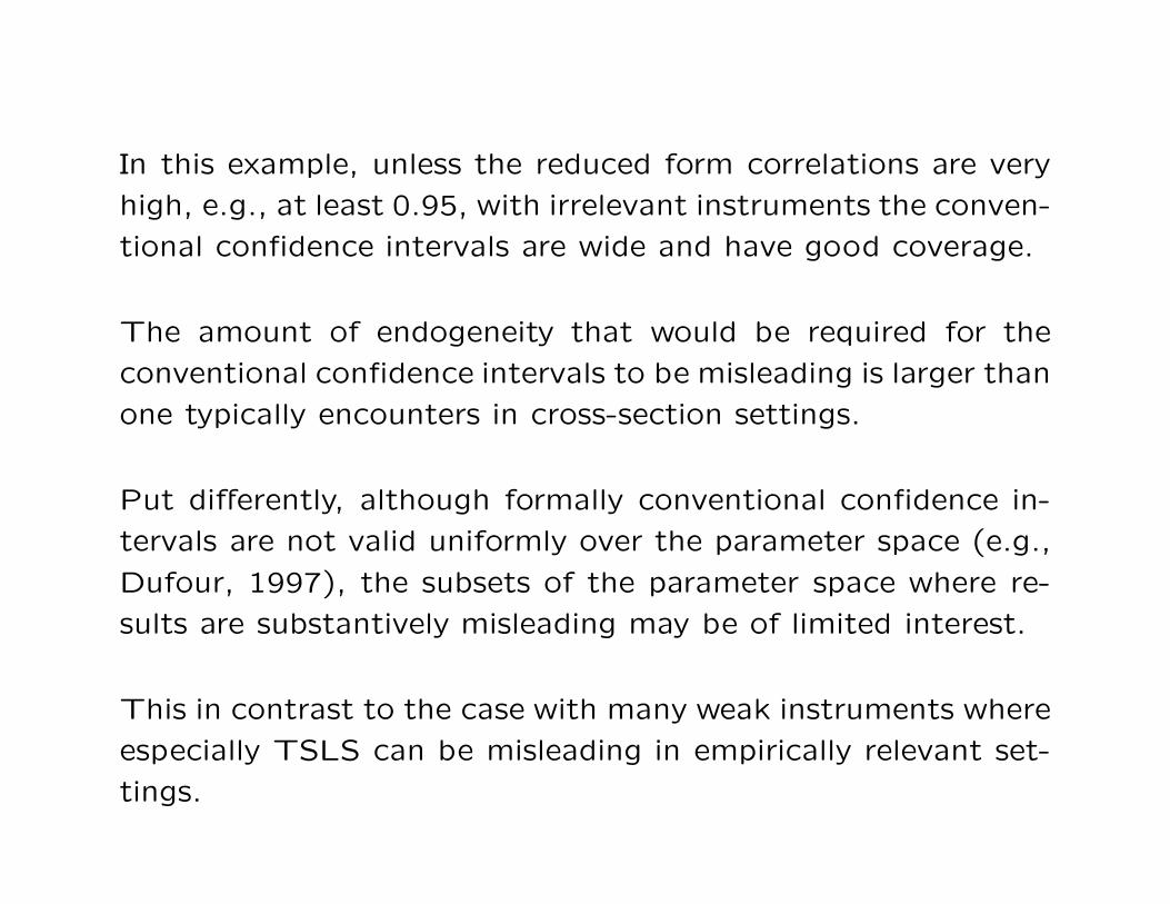
In this example, unless the reduced form correlations are very
high, e.g., at least 0.95, with irrelevant instruments the conven-
tional confidence intervals are wide and have good coverage.
The amount of endogeneity that would be required for the
conventional confidence intervals to be misleading is larger than
one typically encounters in cross-section settings.
Put differently, although formally conventional confidence in-
tervals are not valid uniformly over the parameter space (e.g.,
Dufour, 1997), the subsets of the parameter space where re-
sults are substantively misleading may be of limited interest.
This in contrast to the case with many weak instruments where
especially TSLS can be misleading in empirically relevant set-
tings.

3.A Single Weak Instrument
Yi = β0 + β1 · Xi + εi,
Xi = π0 + π1 · Zi + ηi,
with (εi, ηi) ⊥⊥ Zi, and jointly normal with covariance matrix Σ.
The reduced form for the first equation is
Yi = α0 + α1 · Zi + νi,
where the parameter of interest is β1 = α1/π1. Let
Ω = E
(
νiηi
)·(
νiηi
)′ , and Σ = E
(
εiηi
)·(
εiηi
)′ ,
13

Standard IV estimator:
βIV1 =
1N
∑Ni=1
(Yi − Y
) (Zi − Z
)
1N
∑Ni=1
(Xi − X
) (Zi − Z
),
Concentration parameter:
λ = π21 ·
N∑
i=1
(Zi − Z
)2/σ2
η .
14
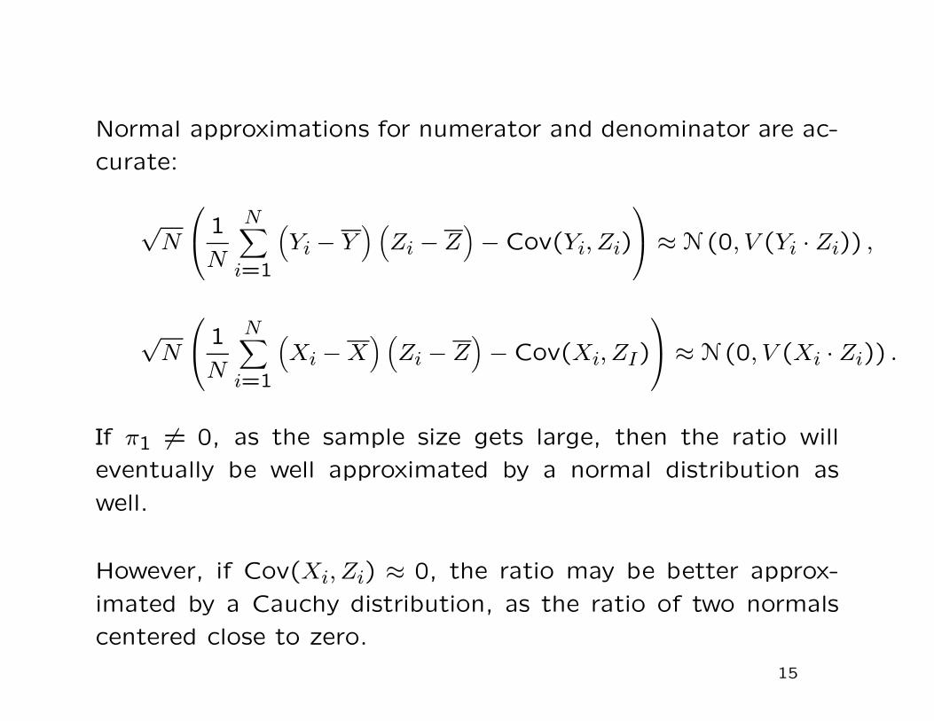
Normal approximations for numerator and denominator are ac-
curate:
√N
1
N
N∑
i=1
(Yi − Y
) (Zi − Z
)− Cov(Yi, Zi)
≈ N (0, V (Yi · Zi)) ,
√N
1
N
N∑
i=1
(Xi − X
) (Zi − Z
)− Cov(Xi, ZI)
≈ N (0, V (Xi · Zi)) .
If π1 6= 0, as the sample size gets large, then the ratio will
eventually be well approximated by a normal distribution as
well.
However, if Cov(Xi, Zi) ≈ 0, the ratio may be better approx-
imated by a Cauchy distribution, as the ratio of two normals
centered close to zero.
15
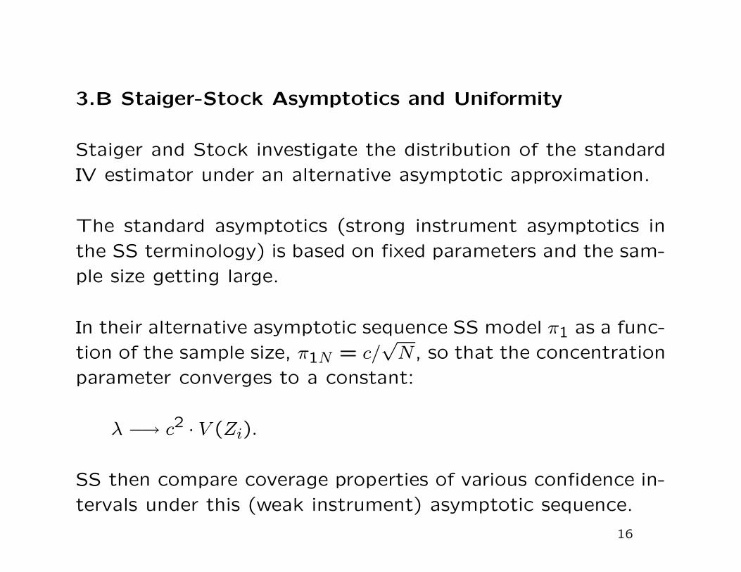
3.B Staiger-Stock Asymptotics and Uniformity
Staiger and Stock investigate the distribution of the standard
IV estimator under an alternative asymptotic approximation.
The standard asymptotics (strong instrument asymptotics in
the SS terminology) is based on fixed parameters and the sam-
ple size getting large.
In their alternative asymptotic sequence SS model π1 as a func-
tion of the sample size, π1N = c/√
N, so that the concentration
parameter converges to a constant:
λ −→ c2 · V (Zi).
SS then compare coverage properties of various confidence in-
tervals under this (weak instrument) asymptotic sequence.
16
The importance of the SS approach is in demonstrating for
any sample size there are values of the nuisance parameters
such that the actual coverage is substantially away from the
nominal coverage.
More recently the issue has therefore been reformulated as re-
quiring confidence intervals to have asymptotically the correct
coverage probabilities uniformly in the parameter space. See
for a discussion from this perspective Mikusheva.
Note that there cannot exist estimators that are consistent for
β∗ uniformly in the parameter space since if π1 = 0, there are
no consistent estimators for β1. However, for testing there are
generally confidence intervals that are uniformly valid, but they
are not of the conventional form, that is, a point estimate plus
or minus a constant times a standard error.
17
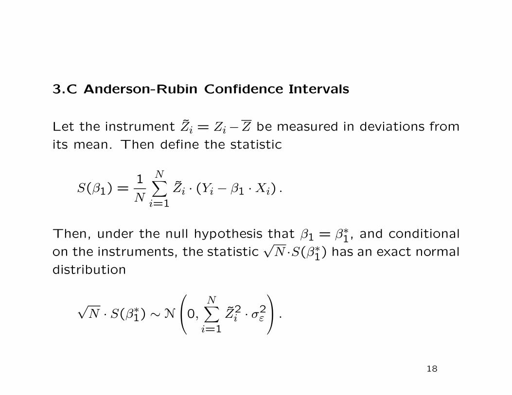
3.C Anderson-Rubin Confidence Intervals
Let the instrument Zi = Zi −Z be measured in deviations from
its mean. Then define the statistic
S(β1) =1
N
N∑
i=1
Zi · (Yi − β1 · Xi) .
Then, under the null hypothesis that β1 = β∗1, and conditional
on the instruments, the statistic√
N ·S(β∗1) has an exact normal
distribution
√N · S(β∗
1) ∼ N
0,
N∑
i=1
Z2i · σ2
ε
.
18
Anderson and Rubin (1949) propose basing tests for the null
hypothesis
H0 : β1 = β01, against the alternative hypothesis Ha : β1 6= β0
1
on this idea, through the statistic
AR(β01
)=
N · S(β01)
2
∑Ni=1 Z2
i
·((
1 −β01
)Ω
(1
−β01
))−1
.
A confidence interval can be based on this test statistic by
inverting it:
CIβ10.95 = β1 |AR(β1) ≤ 3.84
This interval can be equal to the whole real line. Not attrac-
tive from a Bayesian perspective.
19
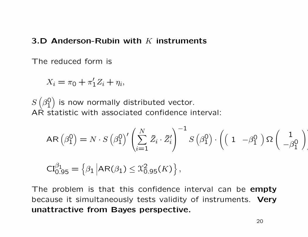
3.D Anderson-Rubin with K instruments
The reduced form is
Xi = π0 + π′1Zi + ηi,
S(β01
)is now normally distributed vector.
AR statistic with associated confidence interval:
AR(β01
)= N · S
(β01
)′
N∑
i=1
Zi · Z′i
−1
S(β01
)·((
1 −β01
)Ω
(1
−β01
))
CIβ10.95 =
β1
∣∣∣AR(β1) ≤ X20.95(K)
,
The problem is that this confidence interval can be empty
because it simultaneously tests validity of instruments. Very
unattractive from Bayes perspective.
20
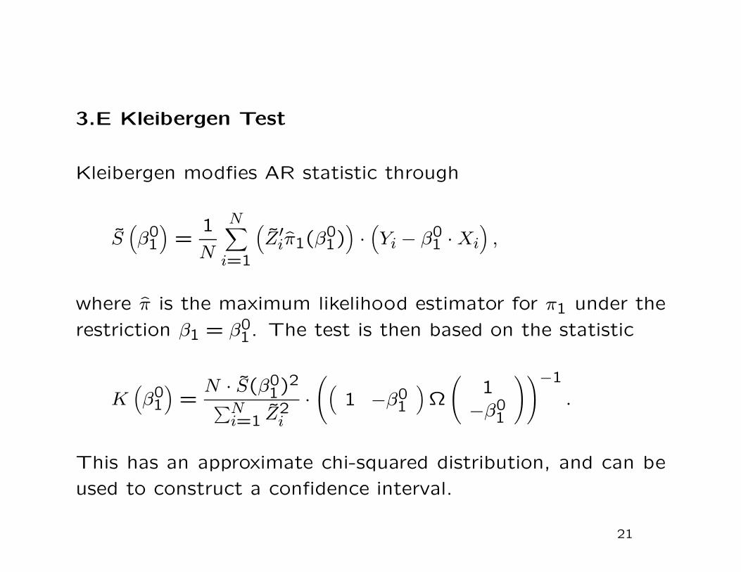
3.E Kleibergen Test
Kleibergen modfies AR statistic through
S(β01
)=
1
N
N∑
i=1
(Z′
iπ1(β01))·(Yi − β0
1 · Xi
),
where π is the maximum likelihood estimator for π1 under the
restriction β1 = β01. The test is then based on the statistic
K(β01
)=
N · S(β01)
2
∑Ni=1 Z2
i
·((
1 −β01
)Ω
(1
−β01
))−1
.
This has an approximate chi-squared distribution, and can be
used to construct a confidence interval.
21

3.F Moreira’s Similar Tests
Moreira (2003) proposes a method for adjusting the critical
values that applies to a number of tests, including the Kleiber-
gen test. His idea is to focus on similar tests, test that have
the same rejection probability for all values of the nuisance pa-
rameter (the π) by adjusting critical values (instead of using
quantiles from the chi-squared distribution).
The way to adjust the critical values is to consider the distribu-
tion of a statistic such as the Kleibergen statistic conditional
on a complete sufficient statistic for the nuisance parameter.
In this setting a complete sufficient statistic is readily available
in the form of the maximum likelihood estimator under the
null, π1(β01).
22
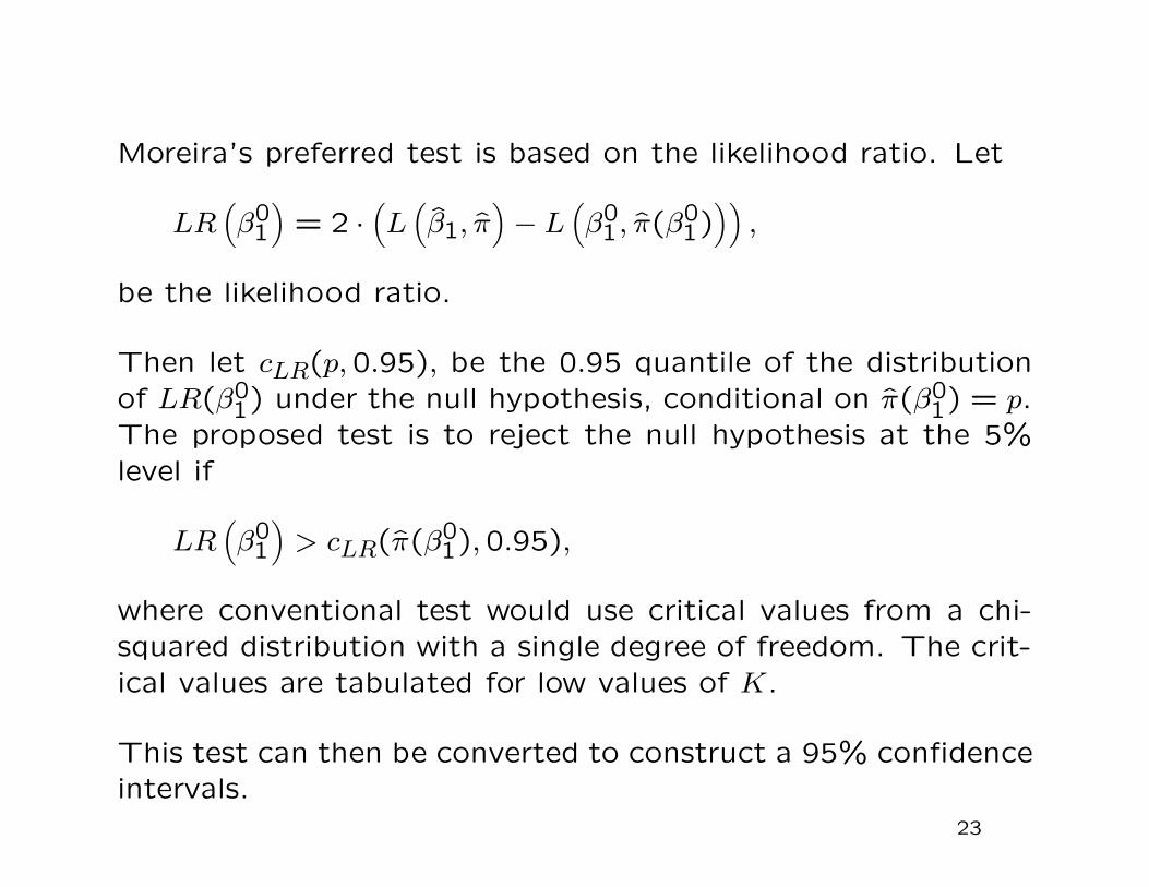
Moreira’s preferred test is based on the likelihood ratio. Let
LR(β01
)= 2 ·
(L(β1, π
)− L
(β01, π(β0
1)))
,
be the likelihood ratio.
Then let cLR(p, 0.95), be the 0.95 quantile of the distribution
of LR(β01) under the null hypothesis, conditional on π(β0
1) = p.
The proposed test is to reject the null hypothesis at the 5%
level if
LR(β01
)> cLR(π(β0
1), 0.95),
where conventional test would use critical values from a chi-
squared distribution with a single degree of freedom. The crit-
ical values are tabulated for low values of K.
This test can then be converted to construct a 95% confidence
intervals.
23

3.G Conditioning on the First Stage
These confidence intervals are asymptotically valid irrespective
of the strength of the first stage (the value of π1). However,
they are not valid if one first inspects the first stage, and con-
ditional on the strength of that, decides to proceed.
Specifically, if in practice one first inspects the first stage, and
decide to abandon the project if the first stage F-statistic is
less than some fixed value, and otherwise proceed by calculat-
ing confidence interval, the large sample coverage probabilities
would not be the nominal ones.
Chioda and Jansson propose a confidence interval that is valid
conditional on the strength of the first stage. A caveat is that
this involves loss of information, and thus the Chioda-Jansson
confidence intervals are wider than confidence intervals that
are not valid conditional on the first stage.
24

4.A Many (Weak) Instruments
In this section we discuss the case with many weak instruments.
The problem is both the bias in the standard estimators, and
the misleadingly small standard errors based on conventional
procedures, leading to poor coverage rates for standard confi-
dence intervals in many situations.
Resampling methods such as bootstrapping do not solve these
problems.
The literature has taken a number of approaches. Part of
the literature has focused on alternative confidence intervals
analogues to the single instrument case. In addition a variety
of new point estimators have been proposed.
Generally LIML still does well, but standard errors need to be
adjusted.
25
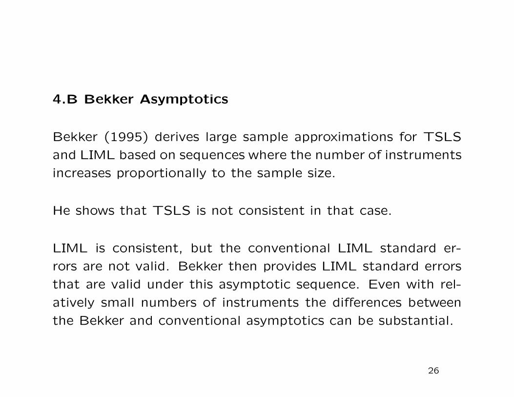
4.B Bekker Asymptotics
Bekker (1995) derives large sample approximations for TSLS
and LIML based on sequences where the number of instruments
increases proportionally to the sample size.
He shows that TSLS is not consistent in that case.
LIML is consistent, but the conventional LIML standard er-
rors are not valid. Bekker then provides LIML standard errors
that are valid under this asymptotic sequence. Even with rel-
atively small numbers of instruments the differences between
the Bekker and conventional asymptotics can be substantial.
26
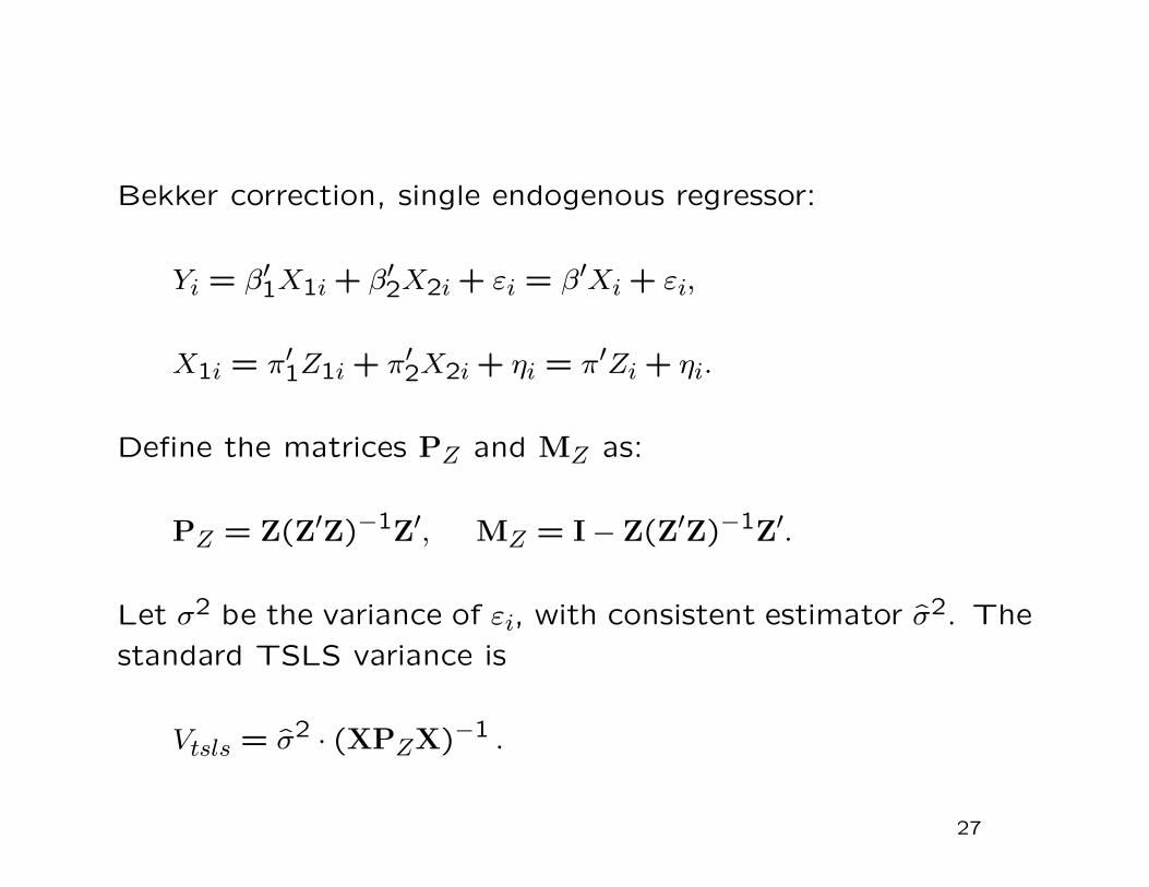
Bekker correction, single endogenous regressor:
Yi = β′1X1i + β′
2X2i + εi = β′Xi + εi,
X1i = π′1Z1i + π′
2X2i + ηi = π′Zi + ηi.
Define the matrices PZ and MZ as:
PZ = Z(Z′Z)−1
Z′, MZ = I − Z(Z′
Z)−1Z′.
Let σ2 be the variance of εi, with consistent estimator σ2. The
standard TSLS variance is
Vtsls = σ2 · (XPZX)−1 .
27
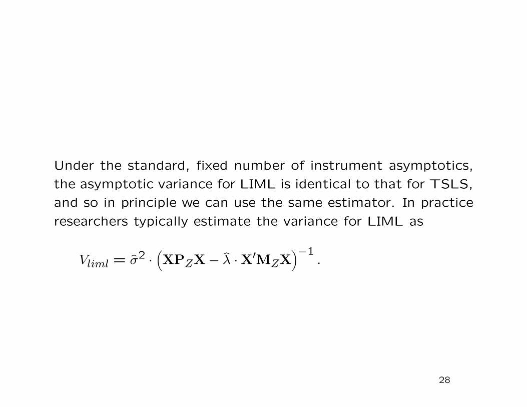
Under the standard, fixed number of instrument asymptotics,
the asymptotic variance for LIML is identical to that for TSLS,
and so in principle we can use the same estimator. In practice
researchers typically estimate the variance for LIML as
Vliml = σ2 ·(XPZX − λ · X′
MZX
)−1.
28

To get Bekker’s correction, we need a little more notation.
Define
Ω =(
Y X
)PZ
(Y X
)/N =
(Ω11 Ω12Ω′
12 Ω22
),
Ω11 = YPZY/N, Ω12 = YPZX/N, and Ω22 = XPZX/N.
A = N · Ω′12Ω12 − Ω22βΩ12 − Ω′
12β′Ω22 + Ω22ββ′Ω22
Ω11 − 2Ω12β + β′Ω22β.
Then:
Vbekker = σ2 ·(XPZX − λ · X′
MZX
)−1
× (XPZX − λ · A) ·(XPZX − λ · X′
MZX
)−1.
Recommended in practice
29
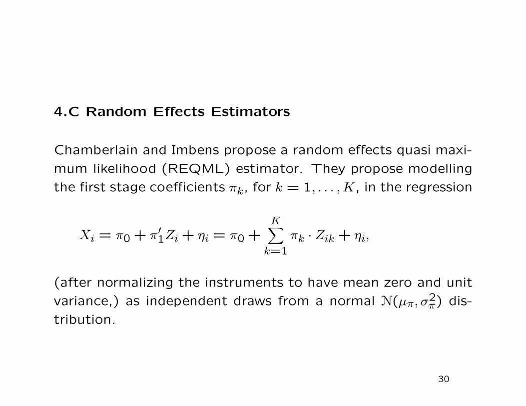
4.C Random Effects Estimators
Chamberlain and Imbens propose a random effects quasi maxi-
mum likelihood (REQML) estimator. They propose modelling
the first stage coefficients πk, for k = 1, . . . , K, in the regression
Xi = π0 + π′1Zi + ηi = π0 +
K∑
k=1
πk · Zik + ηi,
(after normalizing the instruments to have mean zero and unit
variance,) as independent draws from a normal N(µπ, σ2π) dis-
tribution.
30

Assuming also joint normality for (εi, ηi), one can derive the
likelihood function
L(β0, β1, π0, µπ, σ2π,Ω).
In contrast to the likelihood function in terms of the original
parameters (β0, β1, π0, π1,Ω), this likelihood function depends
on a small set of parameters, and a quadratic approximation
to its logarithms is more likely to be accurate.
31
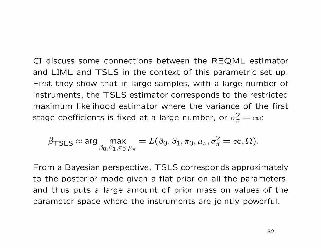
CI discuss some connections between the REQML estimator
and LIML and TSLS in the context of this parametric set up.
First they show that in large samples, with a large number of
instruments, the TSLS estimator corresponds to the restricted
maximum likelihood estimator where the variance of the first
stage coefficients is fixed at a large number, or σ2π = ∞:
βTSLS ≈ arg maxβ0,β1,π0,µπ
= L(β0, β1, π0, µπ, σ2π = ∞,Ω).
From a Bayesian perspective, TSLS corresponds approximately
to the posterior mode given a flat prior on all the parameters,
and thus puts a large amount of prior mass on values of the
parameter space where the instruments are jointly powerful.
32

In the special case where we fix µπ = 0, and Ω is known, andthe random effects specification applies to all instruments, CIshow that the REQML estimator is identical to LIML.
However, like the Bekker asymptotics, the REQML calculationssuggests that the standard LIML variance is too small: thevariance of the REQML estimator is approximately equal tothe standard LIML variance times
1 + σ−2π ·
(
1β1
)′Ω−1
(1β1
)−1
.
This is similar to the Bekker adjustment if we replace σ2π by∑
i=1(π′1Zi)
2(K ·N) (keeping in mind that the instruments havebeen normalized to have unit variance).
In practice the CI adjustment will be bigger than the Bekker ad-justment because the ml estimator for σ2
π will take into accountnoise in the estimates of the π, and so σ2
π <∑
i=1(π′1Zi)
2(K ·N).
33

4.D Choosing the Number of Instruments
Donald and Newey (2001) consider the problem of choosing a
subset of an infinite sequence of instruments.
They assume the instruments are ordered, so that the choice
is the number of instruments to use.
The criterion they focus on is based on an estimable approx-
imation to the expected squared error. version of this leads
to approximately the same expected squared error as using the
infeasible criterion.
Although in its current form not straightforward to implement,
this is a very promising approach that can apply to many related
problems such as generalized method of moments settings with
many moments.
34
4.E Flores’ Simulations
In one of the more extensive simulation studies Flores-Lagunes
reports results comparing TSLS, LIML, Fuller, Bias corrected
versions of TSLS, LIML and Fuller, a Jacknife version of TSLS
(Hahn, Hausman and Kuersteiner), and the REQML estimator,
in settings with 100 and 500 observations, and 5 and 30 in-
struments for the single endogenous variable. Does not include
LIML with Bekker standard errors.
He looks at median bias, median absolute error, inter decile
range, coverage rates.
He concludes that “our evidence indicates that the random-
effects quasi-maximum likelihood estimator outperforms alter-
native estimators in terms of median point estimates and cov-
erage rates.”
35

Econometrics of Cross Section and Panel DataLecture 16: Quantile Regression
Jeff WooldridgeMichigan State University
cemmap/PEPA, June 2014
1. Why Quantile Regression?2. Means, Medians, and Quantiles3. Asymptotic Results4. Quantile Regression with Endogenous ExplanatoryVariables
5. Quantile Regression for Panel Data6. Quantile Methods for Corner Solutions
1

1. Why Quantile Regression?
∙ Often want to know the effect of changing a covariate –such as a policy intervention – on features of the distributionother than the mean.∙ How does eligibility in a pension plan affect total wealth atdifferent quantiles of the wealth distribution? The meaneffect may mask very different effects in different parts ofthe wealth distribution.
2
∙ Sometimes we can estimate parameters in underlyingmodels under weaker assumptions using zero conditionalmedian restrictions (rather than zero conditional meanrestrictions).∙Manipulations with medians (and quantiles) are useful forcertain corner solution models, too.
3
2. Means, Medians, and Quantiles∙ Start with a linear population model, where is K 1:
y x u. (1)
∙ Assume Eu2 , so that the distribution of u is not toospread out. (So, for example, we rule out a Cauchydistribution for u, or a t2 distribution.)
4
∙ Ordinary Least Squares (OLS) Estimation:
mina,b∑i1
N
yi − a − xib2. (2)
∙ Least Absolute Deviations (LAD) Estimation:
mina,b∑i1
N
|yi − a − xib|. (3)
5
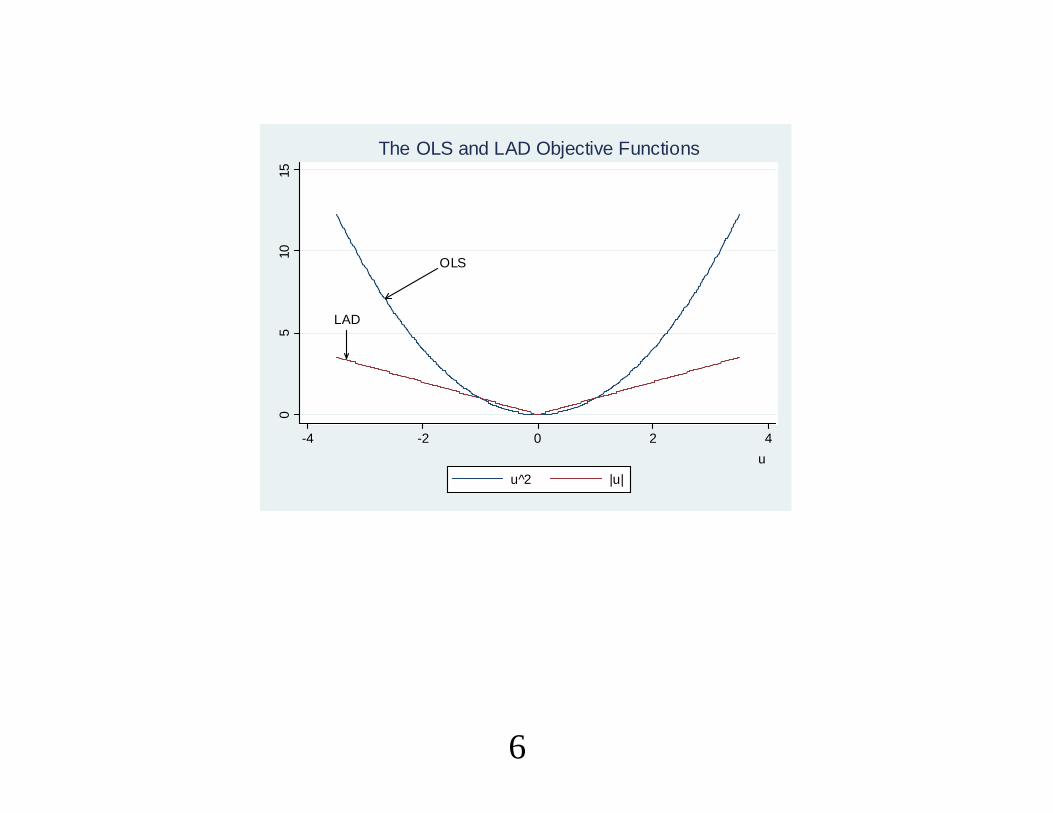
OLS
LAD
05
1015
-4 -2 0 2 4u
u^2 |u|
The OLS and LAD Objective Functions
6

∙ Question: With a large random sample, when should weexpect the slope estimates from OLS and LAD to besimilar?∙ Technically, we are asking when the plims of the slopesare the same.∙ There are two important cases.
7
(i) If
Du|x is symmetric about zero (4)
then OLS and LAD both consistently estimate and
because, under (4), Eu|x Medu|x 0.∙ Consequently,
Ey|x xMedy|x x
8
∙ OLS under random sampling consistently estimates theparameters in a conditional mean.∙ Other than ruling out perfect collinearity in x, sufficientmoment conditions are Eu2 and Exj2 .
∙ Under fairly weak conditions, LAD consistently estimatesthe parameters in a conditional median.
9

(ii) If
u is independent of x with Eu 0, (5)
then OLS and LAD both consistently estimate the slopes, .
∙ By (5), Ey|x x.
∙ If u has an asymmetric distribution, thenMedu ≡ ≠ 0,
and LAD converges to because
Medy|x x Medu|x x x.
10
∙ In many applications, neither (4) nor (5) is likely to betrue. For example, y may be a measure of wealth, in whichcase the error distribution is probably asymmetric andVary|x not constant.∙ If Du|x is asymmetric and changes with x, then weshould not expect OLS and LAD to deliver similar estimatesof , even for “thin-tailed” distributions.
11

∙ Advantage for median over mean: median passes throughmonotonic functions. If
logy x u, Medu|x 0
then
Medy|x exp x
∙ By contrast, we cannot generally find
Ey|x exp xEexpu|x.
12
∙ Expectation has useful properties that the median does not:linearity and the law of iterated expectations.∙ Random coefficient example. If
yi ai xibi (6)
and ai,bi is independent of xi, then
Eyi|xi Eai|xi xiEbi|xi ≡ xi, (7)
where Eai and Ebi.
∙ OLS is consistent for and .
13
∙What can we add so that LAD estimates something ofinterest in (7)? If ui is a vector, then its distributionconditional on xi is centrally symmetric ifDui|xi D−ui|xi.∙ If gi is any vector function of xi, Dgi′ui|xi has a
univariate distribution that is symmetric about zero. Thisimplies Eui|xi 0.
14

∙Write
yi xi ai − xibi − . (8)
If ci ai,bi given xi is centrally symmetric then LADapplied to the usual model yi xi ui consistently
estimates and .
∙ Symmetry of a multivariate distribution is a very strongassumption.
15
Quantiles∙ For 0 1, q is a th quantile of yi ifPyi ≤ q ≥ and Pyi ≥ q ≥ 1 − .∙When yi is continuous with a strictly increasing CDF, qis the unique value such that
Pyi ≤ q
Pyi ≥ q Pyi q 1 − .
∙ If Fy is a strictly increasing CDF then q Fy−1.
16
.75
.51
0
F(y)
0 5 10q(.75) = 3.6y
17
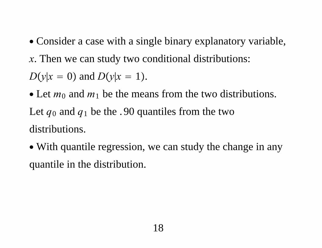
∙ Consider a case with a single binary explanatory variable,x. Then we can study two conditional distributions:Dy|x 0 and Dy|x 1.∙ Let m0 and m1 be the means from the two distributions.Let q0 and q1 be the . 90 quantiles from the twodistributions.∙With quantile regression, we can study the change in anyquantile in the distribution.
18
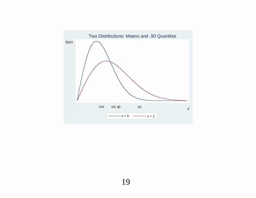
f(y|x)
m0 m1 q0 q1 y
x = 0 x = 1
Two Distributions: Means and .90 Quantiles
19

∙More generally, we are interested in quantiles conditionalon many covariates. Index the parameters by ∈ 0, 1.∙ Assume that the conditional quantile function is uniqueand that it is linear:
Quantyi|xi xi. (9)
20
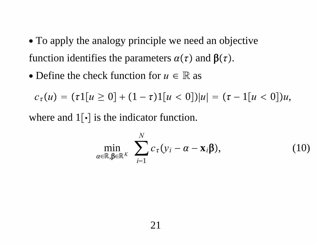
∙ To apply the analogy principle we need an objectivefunction identifies the parameters and .
∙ Define the check function for u ∈ R as
cu 1u ≥ 0 1 − 1u 0|u| − 1u 0u,
where and 1 is the indicator function.
min∈,∈K
∑i1
N
cyi − − xi, (10)
21
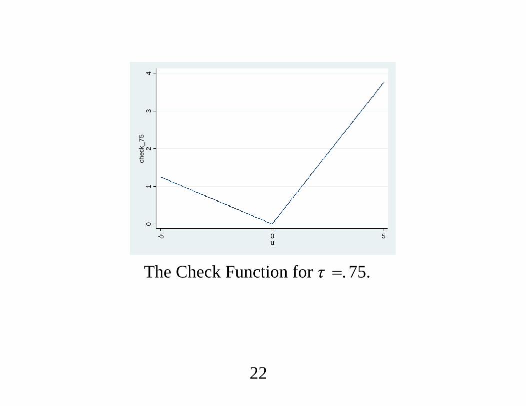
01
23
4ch
eck_
75
-5 0 5u
The Check Function for . 75.
22
3. Asymptotic ResultsConsistency∙ Consistency of QR holds when ui has a continuousdistribution, conditional on xi x. Also fu0|x 0.∙ Purely discrete yi is ruled out.∙ As with OLS, need to rule out perfect collinearity in x.
23

What Happens if the Quantile Function is Misspecified?∙ An important property of OLS: If ∗ and ∗ are the plims
from the OLS regression yi on 1,xi, these provide thesmallest mean squared error approximation to Ey|x x
in that ∗,∗ solve
min,Ex − − x2.
∙ No simple analog for quantile estimation. Some results arein Angrist, Chernozhukov, and Fernández-Val (2006,Econometrica).
24
Asymptotic Inference∙ The asymptotic theory is complicated by the fact that theobjective function is piecewise linear.∙ Nevertheless, quantile regression estimators are
N -asymptotically normal under conditions similar to thosefor consistency.
25
Computing Standard Errors∙ Assume the conditional quantile is linear and put theintercept in xi:
Quantyi|xi xi.
Then
N − a Normal0,A−1BA−1
A Efu0|xixi′xi.
B 1 − Exi′xi.
26
∙ A consistent estimator of B is
B 1 − N−1∑i1
N
xi′xi .
∙ Generally, a consistent estimator of A Efu0|xixi′xi is
 2NhN−1∑i1
N
1|ûi | ≤ hNxi′xi
ûi yi − xi, i 1, . . . ,N.
where hN → 0 and N hN → .
27
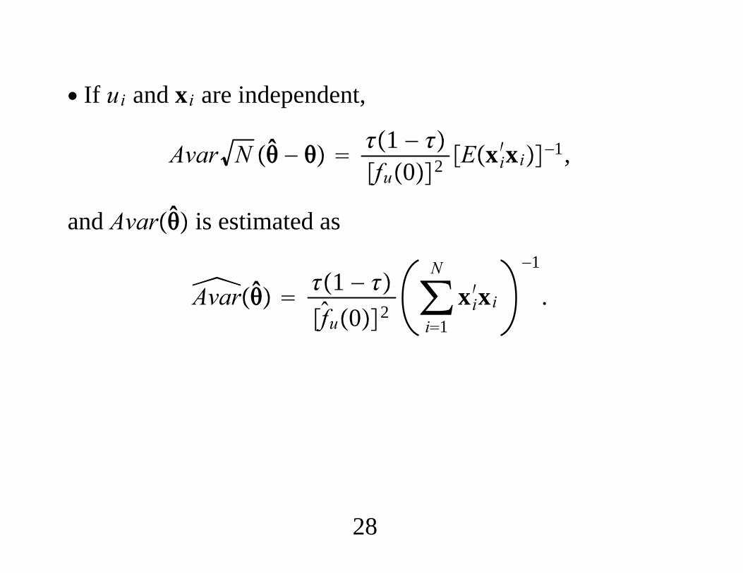
∙ If ui and xi are independent,
Avar N − 1 − fu02 Exi
′xi−1,
and Avar is estimated as
Avar 1 − fu02 ∑
i1
N
xi′xi−1
.
28

∙ The last estimate is commonly reported as the default (byStata).∙ If the quantile function is misspecified we need a differentestimator of B.∙ Kim and White (2002) and Angrist, Chernozhukov, andFernández-Val (2006) show
B N−1∑i1
N
− 1ûi 02xi′xi
is generally consistent for B.
29
∙ Hahn (1995, 1997) shows that the nonparametricbootstrap, where we resample all elements in x,y –generally provides consistent estimates of the fully robustvariance matrix without claims about the conditionalquantile being correct.∙ The bootstrap does not provide “asymptotic refinements”for testing and confidence intervals.
30

Example: Effects of 401(k) eligibility on net financialwealth.∙ Data from Abadie (2003), 401KSUBS.DTA.∙ Outcome variable nettfa is net total financial assets, e401kis a dummy variable indicating eligibility in a 401(k)employer-provided pension plan.
31
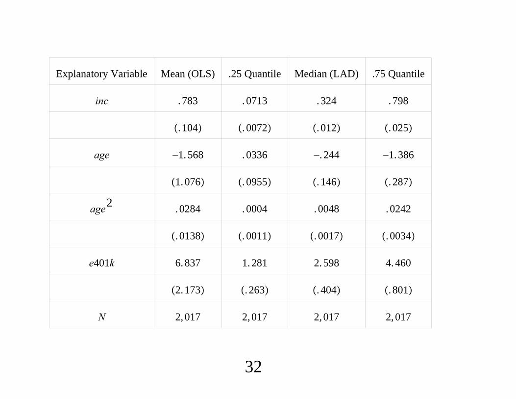
Explanatory Variable Mean (OLS) .25 Quantile Median (LAD) .75 Quantile
inc . 783 .0713 .324 .798
. 104 . 0072 . 012 . 025
age −1.568 .0336 −. 244 −1.386
1.076 . 0955 . 146 . 287
age2 .0284 .0004 .0048 .0242
. 0138 . 0011 . 0017 . 0034
e401k 6.837 1.281 2.598 4.460
2.173 . 263 . 404 . 801
N 2,017 2,017 2,017 2,017
32
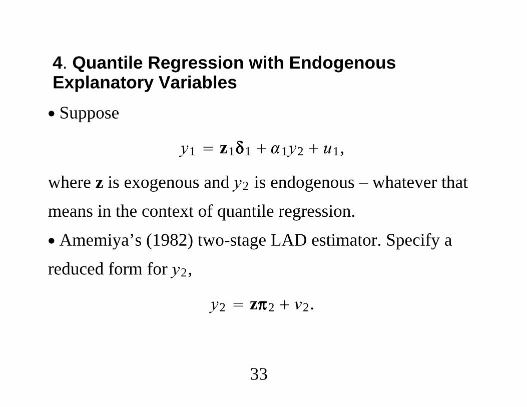
4. Quantile Regression with EndogenousExplanatory Variables∙ Suppose
y1 z11 1y2 u1,
where z is exogenous and y2 is endogenous – whatever thatmeans in the context of quantile regression.∙ Amemiya’s (1982) two-stage LAD estimator. Specify areduced form for y2,
y2 z2 v2.
33
∙ The first step applies OLS to get fitted values, ŷi2 zi2.∙ These are inserted for yi2 to give LAD of yi1 on zi1,ŷi2.∙ Consistency of 2SLAD relies on the median of thecomposite error 1v2 u1 given z being zero, or at leastconstant.
34

∙ If Du1,v2|z is centrally symmetric, can use a controlfunction approach, as in Lee (2007, Journal ofEconometrics).1. Get LAD residuals vi2 yi2 − zi2.2. LAD of yi1 on zi1,yi2, vi2. Use t test on vi2 to test null thaty2 is exogenous.∙ Interpretation of LAD in context of omitted variables isdifficult unless lots of joint symmetry assumed.
35
∙ Discrete y2 is difficult. Point identification holds onlyunder strong assumptions, even when y2 is binary.∙ Cannot just plug in, say, probit fitted values, and then useLAD. Similar comments hold for other discrete y2.∙ Control function approaches with “generalized residuals”may provide good approximations.
36

5. Quantile Regression for Panel Data∙Without unobserved effects, QR easy to extend to paneldata.on panel data:
Quantyit|xit xit, t 1, . . . ,T.
∙ Serial correlation-robust variance matrix estimate for B:
B N−1∑i1
N
∑t1
T
∑r1
T
sitsir′
sit −xit′ − 1yit − xit 0
37

∙ The estimator of A is a natural extension from the crosssection case:
 2NhN−1∑i1
N
∑t1
T
1|ûit|≤ hNxit′ xit
∙ The asymptotic variance of is estimated as Â−1BÂ−1/N.∙ Can use the panel bootstrap, too.
38
Unobserved Effects∙ Explicitly allowing unobserved effects is harder. A strictexogeneity assumption conditional on ci, along withlinearity, gives
Quantyit|xi,ci Quantyit|xit,ci xit ci.
∙ A “fixed effects” approach, where Dci|xi unrestricted, isattractive, but not generally available, except by treating theci as parameters to estimate.
39
∙More flexibility if we start with median,
yit xit ci uit, Meduit|xi,ci 0
1. Apply Honoré (1992): LAD on the first differences isconsistent when uit : t 1, . . . ,T is an iid sequenceconditional on xi,ci (symmetry not required).∙When T 2, LAD on the first differences is equivalent toestimating the ci along with in pooled LAD estimation onlevels.
40

2. Apply LAD to the time-demeaned equation
ÿit xit üit,
using serial correlation-robust standard errors.∙ Consistency follows if üit has a zero conditional median,which holds if Dui|xi,ci is centrally symmetric.∙ Should use serial-correlation-robust inference.
41

∙ If we impose the Chamberlain-Mundlak device,
yit xit xi ai uit,
we can get by with symmetry of Dai uit|xi.∙ Pooled LAD of yit on 1,xit, and xi consistently estimatest,,. Use serial-correlation-robust inference.
∙Might apply general QR to the time-demeaned equation orthe Mundlak equation as an approximation.
42
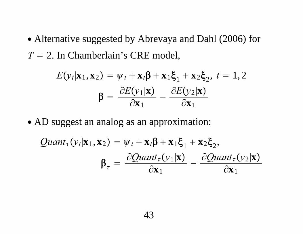
∙ Alternative suggested by Abrevaya and Dahl (2006) forT 2. In Chamberlain’s CRE model,
Eyt|x1,x2 t xt x11 x22, t 1, 2
∂Ey1|x∂x1
− ∂Ey2|x∂x1
∙ AD suggest an analog as an approximation:
Quantyt|x1,x2 t xt x11 x22,
∂Quanty1|x
∂x1− ∂Quanty2|x
∂x1
43
Estimation of the Fixed Effects∙ Treating the ci as parameters results in an incidentalparameters problem. Generally, the bias is of order 1/T.∙ Can use a penalized objective function.∙ Large N, large T theory available, but time series isrestricted. Time dummies often ruled out.∙ Lots of ongoing work.
44
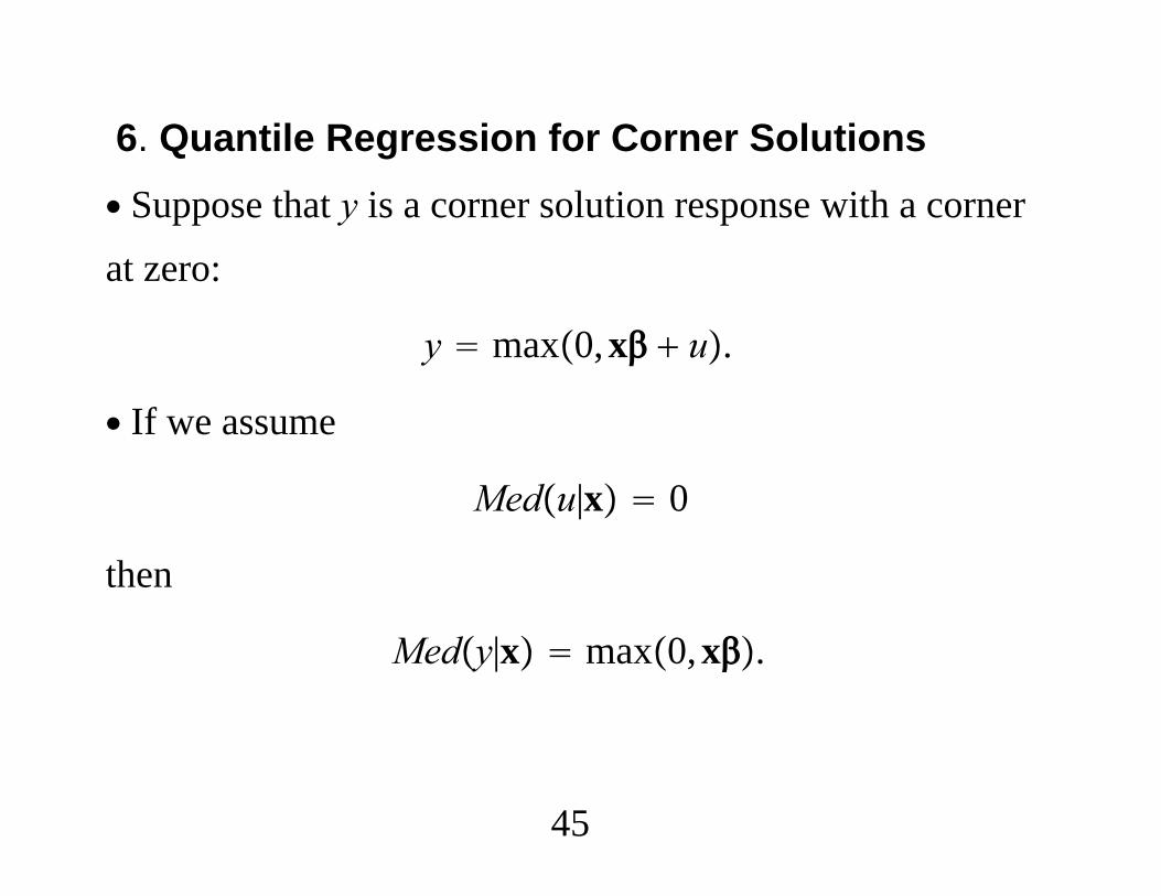
6. Quantile Regression for Corner Solutions∙ Suppose that y is a corner solution response with a cornerat zero:
y max0,x u.
∙ If we assume
Medu|x 0
then
Medy|x max0,x.
45

∙ The zero conditional median restriction on u identifies onefeature of Dy|x, namely, Medy|x.
01
23
-3 -2 -1 0 1 2 3x
median mean
y = max(0,x + u)
46

∙ j measures the partial effect on Medy|x once
Medy|x 0.∙ If xj is continuous,
∂Medy|x∂xj
j1x 0.
∙ Honoré (2008) shows a simple estimator of the average ofthese effects (across the distribution of x is easily
estimated: j where is the fraction of strictly positive yi.
47
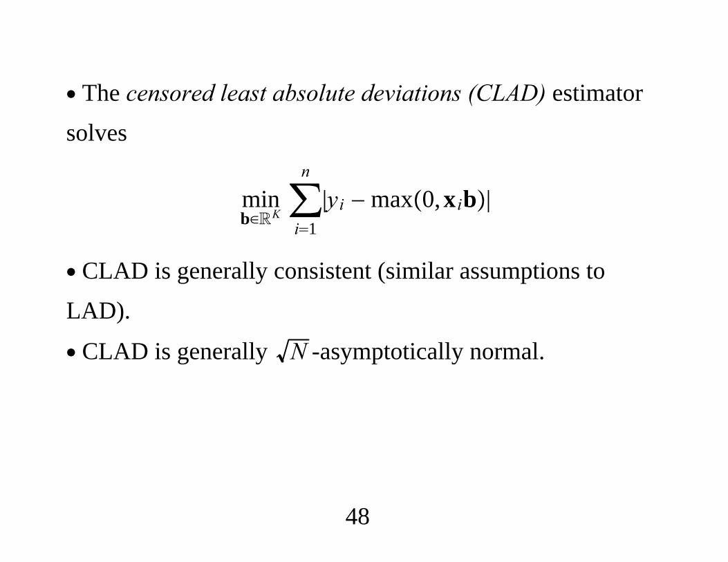
∙ The censored least absolute deviations (CLAD) estimatorsolves
minb∈RK∑i1
n
|yi − max0,xib|
∙ CLAD is generally consistent (similar assumptions toLAD).
∙ CLAD is generally N -asymptotically normal.
48
∙ The standard Tobit model and extensions can berestrictive, but they identify all of Dy|x.∙We could just specify Ey|x and use nonlinear leastsquares or QMLE methods.∙ For corner solution responses there is a tradeoff betweenmaking fewer assumptions and how much can be learned.
49

∙ In the panel case, we can start with
yit max0,xit ci uitMeduit|xi,ci 0, t 1, . . . ,T.
∙ These imply that
Medyit|xi,ci max0,xit ci.
50

∙ Strict exogeneity is assumed.∙ Honoré (1992) showed how to estimate without
restricting Dci|xi by imposing “exchangeability”assumptions on uit : t 1, . . . ,T.∙ It is like a “conditional MLE” for corner solutions; the ciare not treated as parameters to estimate.∙ Heteroskedasticity and other time heterogeneity are ruledout.
51
∙ The partial effect of xtj on Medyit|xit xt,ci c is
tjxt,c 1xt c 0j.
∙What values should we insert for c?∙ Averaging across Dci gives average partial effects on themedian:
tjxt Ecitjxt,ci 1 − Gxtj
where G is the unconditional cdf of ci. Generally notidentified.
52

∙ For APEs, write yt max0,xt vt where vt c ut.
∙ If vt has a continuous distribution, the probability of beingat the kink is zero, so
∂yt∂xtj
xt,vt 1xt vt 0j
and
Ext,vt∂yt∂xtj
xt,vt Pyt 0j
53
∙ Given j – available using methods summarized by
Arellano and Honoré (2001) – the avererage partial effect iseasily estimated as
Pyt 0j tj
t N−1∑i1
N
1yit 0
∙ But we cannot estimate how the partial effects change withxt.
54
∙ Unclear what to do about discrete changes.
∙ If xt1 and xt
0 are two values of xt, we would like to study
max0,xt1 c − max0,xt
0 c,
but we do not know what to plug in for c, or how to averageout across the distribution of c.
55