What Can the Price Gap between Branded and Private-Label

This PDF is a selection from a published volume from theNational Bureau of Economic Research

Volume Title: Scanner Data and Price Indexes

Volume Author/Editor: Robert C. Feenstra and MatthewD. Shapiro, editors

Volume Publisher: University of Chicago Press

Volume ISBN: 0-226-23965-9

Volume URL: http://www.nber.org/books/feen03-1

Conference Date: September 15-16, 2000

Publication Date: January 2003

Title: What Can the Price Gap between Branded and Private-LabelProducts Tell Us about Markups?

Author: Robert B. Barsky, Mark Bergen, Shantanu Dutta,Daniel Levy

URL: http://www.nber.org/chapters/c9736

165

7.1 Introduction

The magnitude of marginal costs and markups over marginal cost areempirical questions of considerable general interest in economics. Micro-economists are interested in markups because they bear on such questionsas the relevance of alternative models of imperfect competition, the welfareconsequences of market power, and the benefits of new product introduc-tion. In recent macroeconomic research as well, markups play a central role(see, e.g., Hall 1986, 1988). Although macroeconomic discourse most oftenfocuses on the cyclicality rather than the level of markups, the degree ofcyclicality is often limited by the absolute size of the markup (Rotembergand Saloner 1986).

7What Can the Price Gap betweenBranded and Private-LabelProducts Tell Us about Markups?

Robert Barsky, Mark Bergen, Shantanu Dutta, and Daniel Levy

Robert Barsky is professor of economics at the University of Michigan and a research asso-ciate of the National Bureau of Economic Research. Mark Bergen is associate professor ofmarketing and logistics management at the Carlson School of Management, University ofMinnesota. Shantanu Dutta is associate professor of marketing at the University of SouthernCalifornia. Daniel Levy is associate professor of economics at Bar-Ilan University and EmoryUniversity.

The authors are grateful to the paper’s discussant, Julio Rotemberg, for his insightful com-ments, which played a fundamental role in the restructuring and strengthening of the argu-ment. Susanto Basu and Matthew Shapiro provided numerous valuable suggestions and es-sential advice. The authors would also like to thank Ning Liu for her outstanding researchassistance under a very tight schedule, Owen Beelders, Ernie Berndt, Hashem Dezhbakhsh,Jim Hess, Kai-uwe Kuhn, Jim Levinsohn, Peter Rossi, and Steve Salant for many helpful dis-cussions, Robert Feenstra for comments, Steve Hoch for providing us with his survey data onnational brand/private-label quality differences, and Jong Kim for his help with computations.They thank the participants of the NBER-CRIW conference, the 2001 Midwest MarketingCamp, and seminar participants at the University of Michigan and the University of Min-nesota. Finally, the authors thank both the Kilts Center for Marketing, Graduate School ofBusiness, University of Chicago, and Dominick’s for providing us with the data. The usual dis-claimers apply.

The estimation of markups is difficult because marginal cost is not di-rectly observable. There are essentially two ways in which inference aboutmarkups and marginal cost is approached in the econometric literature.One approach is via the cost function, which is either inferred directly fromengineering data or estimated from cross-sectional or time series marketdata. The other is to estimate consumer demand functions and compute themarkup based on estimated demand elasticities, in combination with amodel of market equilibrium.

This paper takes a quite different approach to measurement of marginalcosts and markup ratios. We argue that the price of a “private-label” equiv-alent or near-equivalent product provides valuable information about themarginal cost of the nationally branded product. In particular, because theprivate-label version would not sell at a price less than its marginal cost, theratio of the price of the branded product to that of the private-label oneserves as a lower bound on the markup ratio. The high relative price of na-tional brands is thus indicative of substantial markups over marginal cost.

Underlying our approach is the notion that private-label products aremore or less physically identical to nationally branded products, but thebranded product commands a higher market price due to characteristicsnot related to marginal costs of either manufacturing or retail handling.Many of the promotional expenses that vertically differentiate the brandedproduct from its private-label counterpart appear largely as sunk, or at leastfixed, costs. Essentially the same is true of expenditure on research and de-velopment. To the extent that marginal costs of private-label goods divergefrom those of the branded versions, we present evidence that suggests thatmanufacturing costs for the private labels are if anything higher on the mar-gin than those for the corresponding brands.

Informed by the above considerations and in possession of data on bothretail prices and the retailer’s margins over wholesale, we take the wholesaleprice of the private-label product as an upper bound for the marginal man-ufacturing cost of its branded counterpart. The presumption that retailers’margins must at least cover marginal handling costs allows inference aboutthe contribution of the retail channel to full marginal cost. We present sev-eral ratios that, under reasonable assumptions, bound the true marginalcost of manufacturing and selling the branded product from above as wellas below.

We emphasize the lower-bound measure of the true markup. To brieflysummarize our main results, markups computed in this manner are consis-tent with, but on the high side of, those found in previous studies, for thefew products for which such studies exist. Markups for national brands soldin supermarkets are large. Lower bounds on markup ratios measured thisway range from 3.44 for toothbrushes and 2.23 for soft drinks to about1.15–1.20 for canned tuna and frozen entrees, with the majority of cate-gories falling in the range 1.40–2.10.

166 Robert Barsky, Mark Bergen, Shantanu Dutta, and Daniel Levy

The ratio of brand to private-label retail prices has on occasion been usedin the literature as a measure of the markup. The texts by Scherer (1980) andCarlton and Perloff (1994) present some informally collected data of thissort. A recent paper by Nevo (1997) computes the retail price ratio as acheck on structural estimation of markups on breakfast cereals and finds amarkup ratio of about 1.30, very much in accord with the estimates from thestructural approach. Our data indicate, in accord with results from previousstudies, that retailers earn higher margins on private labels than on nationalbrands. This suggests that the retailer’s margin on the branded variety ismost likely the best indicator of actual marginal handling cost at the retaillevel. If this is the case, ratios of retail prices understate national brandmarkups over the “true” marginal cost of providing goods to the consumer.

We apply our approach to products in the grocery industry, in whichthere are many private-label or “store brand” products in a wide variety ofcategories.1 We compute our markup ratios using scanner data from theChicago area supermarket chain Dominick’s Finer Foods. The Dominick’sdata include both retail prices and the retailer’s “margin” (and hence, im-plicitly, wholesale prices) for both national brands and the store brand. Thisallows us to decompose ratios of the retail prices into a manufacturer’smarkup and a retailer’s markup on wholesale prices—an exercise that willprove to be important in our efforts to bound the “true” markup from aboveand below. The product descriptions are sufficiently detailed that we areable to identify many pairs of national brand and private-label offerings thatare comparable in both quality and package size.

The paper is structured as follows. In the next section we present our con-ceptual framework. In subsection 7.2.1, we present a simple vertical differ-entiation model emphasizing the role of sunk advertising costs, consumerheterogeneity, and competition for “niche” in carving out a role for privatelabels and determining the size of the equilibrium markup. In section 7.2.2,we highlight the role of retail stores and point out how advertising and com-petition between retailers leads to an inverse relation between wholesaleand retail margins. In section 7.2.3, the most critical part of the analyticalsection, we develop a set of inequalities involving the various price ratiosand show how we can bound the true markup both above and below.

In section 7.3 we answer some possible objections about the comparabil-ity of national brand and private-label products. Evidence suggests that tothe extent that there are differences, they point in the direction that prices

The Price Gap between Branded and Private-Label Products and Markups 167

1. Fitzell (1998) recounts that private labels go back to the late nineteenth century and grad-ually developed from the sale of bulk commodity staples. From the beginning, the main focusof private-label manufacturers has been on packaged goods—packaged teas, sugar, flour,spices, and so on. Early in the twentieth century, private-label manufacturers expanded theiractivity by offering canned vegetables and fruits, frozen foods, and bakery and dairy productsas well. Later, the private-label industry expanded to include paper products, detergents, deliitems, soft drinks, health and beauty care products, and more recently even “untouchable”products such as cosmetics, baby food, natural health products, and gourmet delicacies.

of private-label products overestimate the marginal cost of nationalbrands—suggesting that our assumptions are in fact conservative. In sec-tion 7.4 we introduce the data and discuss measurement methods. In sec-tion 7.5 we present five different but related markup ratios, covering boththe wholesale and retail levels, for over 230 comparable nationally branded-private-label product pairs representing nineteen categories. Computingthe lower bound on markup ratios developed in section 7.2, we documentthat the markups for national brands are large. In section 7.6 we briefly dis-cuss our findings, linking the variation in the magnitude of the markup ra-tios to the materials share in production cost. We conclude the paper in sec-tion 7.7.

7.2 Inferring Marginal Cost and Markups From Private Labels: Theory

7.2.1 Vertical Differentiation and the Coexistence of Brands and Private Labels

We begin with a very stylized example of a market with two firms, bestthought of as integrated manufacturers and sellers, one producing abranded product, the other offering a physically identical unbranded prod-uct. This example is an adaptation of Tirole (1989, 296–98), which in turnfollows Shaked and Sutton’s (1982) model of vertical differentiation andprice competition. Following Sutton (1991), we regard “perceived quality”as a function of the stock of past advertising A (“brand capital”). No hori-zontal differentiation is possible. The two firms both produce at the con-stant unit cost c. Under conditions that guarantee that the market will sup-port both the branded and the private-label product, we derive productprices (and thus margins) as well as profits for the two firms.

Firm 1 enters the game with a stock of “brand equity” A � A�, which canbe thought of as the return to past expenditure on advertising. Firm 2 hasno brand equity: A2 � 0. Although all consumers prefer the branded prod-uct at the same price, willingness to pay for the characteristics associatedwith the branding differs across individuals. Let this heterogeneity, whichwe might associate either with taste or with income differences, be parame-terized by � ~ U(�0, �1), where �0 � 0, and �1 � �0 � 1. The utility of a type� consumer is U � �(1 � A) – p if the consumer purchases one unit of thegood with brand equity A at price p, and 0 otherwise. The type � consumeris thus indifferent between the branded and the private-label good when�(1 � A�) – p1 � � – p2.

When we use a result from Tirole (1989), demands for the two firms as afunction of the prices p1 and p2 are then

D1( p1, p2) � �1 � �p1 �

A�

p2�, and D2( p1, p2 ) � �

p1 �

A�

p2� � �0 .


As A� becomes large, the products become less and less substitutable, andthe relative demand less and less price-sensitive.

Nash equilibrium occurs when firm i maximizes (pi – c)Di( pi , pj ) with re-spect to pj (i, j � 1, 2). The prices, quantities demanded, and profits in theNash equilibrium are

p1 � c � �2�1

3

� �0� A� p2 � c � �

�1 �

3

2�0� A� � p1

D1� �2�1

3

� �0� D2 � �

�1 �

3

2�0�

�1 ��(2�1 �

9

�0)2 A�

� �2 ��(�1 �

9

2�0)2 A�

�

Thus, the qualitative results are as follows:

• Firm 1, the nationally branded incumbent, charges a higher price thanthe private-label firm 2. However, both charge above marginal cost.

• The excess of price over marginal cost, and the profits of both the brandand the private-label producer, are increasing in the degree of hetero-geneity in the population and in firm 1’s stock of brand capital.2

• Both firms make some profit, although the national brand makes more.

7.2.2 Adding the Retail Sector

The stylized model above illustrates the role of brand capital and het-erogeneous tastes for “perceived quality” in providing a market niche forprivate labels, and their effect on markups, quantity sold, and profits. How-ever, we must now add a specific role for retailers, which are obviously cen-tral to our empirical analysis of the supermarket data. Lal and Narasimhan(1996) construct a model along the lines of the above example, but with twomanufacturing firms, two retailers, and a composite outside good. Theirmodel is intended to explain why under some conditions a manufacturer’sadvertising can “squeeze,” that is, lower the retail margin while simulta-neously increasing the wholesale margin, a point stressed previously bySteiner (1993).

Stores carry many products, and on any given purchase occasion a typi-cal consumer buys only a subset of the products. Retailers, Lal and Nara-simhan (1996) hypothesize, therefore tend to compete more aggressivelybased on the prices of a selected set of well-recognized nationally brandeditems by advertising these prices to consumers. Since the contribution toprofit from any customer is the sum of revenue from advertised and un-advertised items, the intensity of retail competition, as is evident from the


2. That the margin of the private-label supplier is increasing in firm 1’s stock of brand equityreflects the “principle of maximal differentiation,” which is not entirely robust (Tirole 1989).

prices of these items, increases with the amount the consumer will expendon the unadvertised items once at the store. This aggressiveness thereforetranslates into lower retail margins on these selected items since the retail-ers expect that consumers, once inside a store, will also buy non-advertisedproducts on which the retailers receive high margins. Manufacturers who,via advertising, have established a stock of well-recognized products, areable to charge high prices to retailers. The higher margin earned by retailerson their private-label products compared with national brands is an impor-tant feature of the data we examine.

If the retail level of the channel is very competitive, retail margins are notlikely to be much larger than handling costs. Many authors (such as Levy etal. 1998; Levy, Dutta, and Bergen 2002) suggest that the retail grocery in-dustry is indeed very competitive. Retail margins on branded products arein fact very small for most product groups in our data set.

7.2.3 Lower Bounds for Markups: Algebra3

The “ideal” measure of the markup ratio—that which measures the ex-tent to which quantity consumed falls short of the first best optimum—isthe price paid by the consumer relative to the full marginal cost of supply-ing an extra unit. Denote the marginal production cost faced by the brandmanufacturer as cp

b and the marginal cost the retailer faces in stocking andselling the branded product—the “marginal handling cost”—as ch

b.4 The

“full” marginal cost of providing a unit of the branded product is thus

(1) cb � cpb � ch

b.

Consequently, we define the true markup as

(2) ∗ � �cp

b �

prb

chb

� ,

where prb denotes the retail price of the branded product. In this subsection,

we show how to bound this ideal measure in terms of quantities that we areable to observe directly in the data on retail price and store margins.

In line with evidence presented in section 7.3, we postulate that the mar-ginal production cost of the private label (denoted by g) is not less than thatof the brand, that is,

(3) cpb cp

g.

Because the manufacturer of the private label will not normally sell at awholesale price less than its marginal production cost, we have


3. This section owes a major debt to our discussant, Julio Rotemberg. 4. Note that we do not make the assumption that cp

b and chb are constant unit costs. We do not

need this assumption in our empirical work, because we are using price data to make bound-ing arguments rather than to arrive at point estimates of marginal costs. In particular, if thereare fixed costs in production or selling that must be covered, the wholesale price and the retailprice will overestimate marginal costs.

(4) cpg pg

w

Combining equations (3) and (4), we have

(5) cpb pg

w.

Thus, the wholesale price of the private label is an upper bound on the mar-ginal manufacturing cost of the brand.

Likewise, the retailer’s margin on the branded product should at leastcover the marginal handling costs. Letting

(6) mrb � pr

b � pbw,

where pbw denotes the wholesale price of the branded product, we have

(7) chb mr

b.

The degree to which mrb overstates marginal handling costs depends on

the ability of the brand manufacturer to extract, on the margin, the rents as-sociated with its brand equity. In the limit, the brand manufacturer extractsall of the rents, and mr

b equals the retailer’s true marginal handling cost.5

However, since we are seeking lower bounds for the “true” markup, the logicof our argument does not in any way depend on such an assumption. Ourbounds will of course be tighter if the marginal profit earned by the store onbrand name goods is small. This is normally the case in practice since, as wewill see in section 7.5, for all but a few product categories the observed mr

b—which must be the sum of true marginal handling cost and the store’s mar-ginal profit—is itself small.

Adding equations (5) and (7), we see that

(8) cb � cpb � ch

b pgw � mr

b.

Define a new ratio as

(9) � �pg

w �

prb

mrb

� ��pg

w �

p

p

rb

rb � pb

w� ,

where the latter equality follows from equation (6). Recalling the definitionof the unobservable “true” markup as ∗ � pr

b /cpb � ch

b from equation (2),the inequality in equation (8) implies that

(10) ∗.

Equation (10) is the result most central to our empirical analysis because itimplies that is a lower bound on the “true” or “ideal” markup. Moreover,


5. There exist some handling cost data in marketing studies that focus on direct productprofitability issues. Although we have not yet obtained these cost data, they would allow us tosee just how conservative our assumptions about handling costs are. Because our primary fo-cus in this paper is on constructing a lower bound on the “ideal” markup, the main thrust ofthe paper would remain unchanged. See Chen et al. (1999) and Marsh Super Study Special Re-port (Progressive Grocer, December 1992 and January 1993) for details. We thank Jim Hess forinforming us about the existence of such data.

it shows how to construct a lower bound on the markup ratio using data di-rectly available in the Dominick’s data set. We will refer to the ratio as ourpreferred lower-bound markup because, as we show immediately below, it isa tighter lower bound for ∗ than is the ratio of the retail prices.

7.2.4 Relationship of and to Retail and Wholesale Price Ratios

It is interesting to compare the preferred markup measure to the retailprice ratio pr

b /prg and to the wholesale price ratio pb

w/pgw—the former because

retail prices are available in a wide variety of data sets (whereas data on re-tailer’s margins are less common), and the latter because it is a lower boundfor the manufacturer’s markup over marginal production cost; that is, pb

w/pgw

pbw/cp

b. Let mrg � pr

g – pgw. As section 7.5 shows, in the data it is almost al-

ways the case that

(11) mrb mr

g,

that is, the retailer earns less revenue net of the wholesale price from sellinga unit of the national brand than from selling a unit of the comparableprivate label. When equation (11) holds, we can see, by combining equa-tions (8) and (11), and using equations (5) and (7), that

(12) cb � cpb � ch

b cpb � mr

b pgw � mr

g � prg .

The retail price of the private label is an upper bound for the full marginalcost of the brand; it is, however, a less tight upper bound than the preferredmarginal cost measure that appears in the denominator of . Hence, themarkup measure based on retail prices, r � pr

b /prg, is a lower bound for the

true markup ∗ and understates ∗ to a greater extent than does . Finally, it is easy to see that the markup measure based on wholesale

prices, w � pbw/pg

w, satisfies w � . Recall that � prb/pg

w � mrb. To go from

to w, we subtract mrb from both the numerator and the dominator. Since

markup ratios exceed unity, the subtraction has a larger percentage effecton the denominator than the numerator. It is not, however, possible to saythat w is unambiguously an upper bound for ∗, because we don’t knowthe extent to which pg

w and mrb exceed, respectively, the true marginal pro-

duction cost and marginal handling cost of the national brand. In summary, we report five markup ratios:

1. � prb /pg

w � mrb, the “preferred” lower-bound measure of the full

markup on the brand,2. r � pr

b /prg, the lower-bound measure of the full markup based on re-

tail prices,3. w � pb

w/pgw, the lower-bound measure of the manufacture’s markup ra-

tio based on wholesale prices, 4. b � pr

b/pbw � mr

b /pbw � 1, the “retailer’s markup” ratio on the brand,

and finally,5. g � pr

g /pgw � mr

g /pgw � 1, the “retailer’s markup” ratio on the private label.


The first three ratios, along with the “true” underlying markup ratio ∗ �pr

b /cpb � ch

b, satisfy the inequalities

r w

and

r ∗.

In table 7.1, we summarize the algebraic notation used in this section forderiving the lower bounds on the markup ratio.

7.3 Branded and Private-Label Products: Issues of Comparability

In section 7.2, we established algebraic conditions under which the ratioswe report can be considered lower bounds on the true markup. The useful-ness of our arguments depends, however, on the maintained hypothesis thatneither the marginal production cost nor the marginal handling cost of thebranded product exceeds that of the private-label version. The appropriate-ness of this assumption is an empirical question whose answer may differacross product categories. In this section we consider three potential objec-tions to the approach in this paper:

• Private-label goods are inferior products produced at lower cost usingcheap, low-quality inputs (the “physical quality” objection).

• Differences in production technique, scale, and factor prices makevariable costs in the manufacturing process noncomparable even whenthe final outputs are comparable (the “production method” objection).

• Even if the private-label product is physically comparable to the na-tionally branded version, the activities of advertising and otherwise


Table 7.1 Notation Used in Deriving the Lower Bounds for Markups

cpb Marginal production cost of the branded product

cpg Marginal production cost of private label

chb Retailer’s “marginal handling cost” of the branded product

cb The “Full” marginal cost of providing a unit of the branded productpr

b Retail price of the branded productpr

g Retail price of private labelpg

w Wholesale price of private labelpb

w Wholesale price of the branded productmr

b Retailer’s margin on branded productmr

g Retailer’s margin on private label∗ The “true” or the “ideal” markup The “preferred” lower bound on the “true” markupr The lower-bound markup based on retail pricesw The lower-bound markup based on wholesale pricesb The retailer’s markup on the branded productg The retailer’s markup on private label

promoting the national brand (and perhaps also expenditures on re-search and development) may create additional marginal costs for na-tional brands (the “marketing cost” objection).

All three of these objections concern the comparability of the nationalbrand and the store brand versions, and all potentially call into question thesupposition that marginal production and marketing costs for the private-label product are at least as great as those for their branded counterparts. Inthe three subsections that we follow, we take up these objections in turn.

7.3.1 Physical Quality

This subsection has two purposes. First, it presents evidence that private-label products are not in general of lower physical quality than the corre-sponding national brands. For the purposes of this paper, this is of interestnot in and of itself, but because a finding of low quality in tests by qualitycontrol managers and consumer organizations might indicate the use oflower quality inputs, and hence lower marginal cost.

Second, although private-label products are not in general physically in-ferior, there is some evidence of variation in the relative quality of brandsand private labels across product categories. Thus we discuss in this sectionour efforts to weed out categories in which there are in fact problems ofcomparability that make it difficult to construct matching pairs of physi-cally identical products.

Branded and private-label versions of a product cannot be economicallyidentical, as that would violate the law of one price. The first objection fromthe earlier list concerns possible differences in the quality of the physicalproduct and not differences in “perceived quality” associated with sunk ad-vertising costs, as discussed by Sutton (1991). Further, because the relevantconcern is with differences in marginal costs, it is in fact not necessary thatthe private-label product be of equal physical quality in all respects. Supe-rior designs or propriety formulas that do not affect marginal cost do notpose a problem. We focus on “quality” to the extent that low quality of theprivate-label product is suggestive of the use of lower cost inputs. We iden-tify product categories in which this appears to be an issue, and we avoidthese in the empirical work reported in sections 7.4 and 7.5.

Hoch and Banerji (1993) note the absence of a secondary data source onprivate-label quality comprehensive enough to cover all the SAMI (SellingAreas Marketing, Inc.) product categories. For example, Consumer Reportsdoes not have quality ratings for all the products included in our data set.Therefore, it undertook a survey of quality assurance managers at the fiftylargest supermarket chains and grocery wholesalers in the United States(according to Thomas Food Industry Register). These experts typically havea graduate education in food science and wide experience testing numerousproduct categories. For each of the original SAMI categories the managers


were asked: “How does the quality of the best private-label supplier com-pare to the leading national brands in the product category?” The respon-dents gave a rating on a five-point scale: a “1” suggests that private labelsare much worse in quality than the national brands, whereas a “5” suggeststhat the private-label quality is fully comparable to that of the nationalbrand.6 In table 7.2, we report the means of these survey-based quality rat-ings for each of the categories that we examine in the Dominick’s data.

Hoch and Banerji’s (1993, 62) own evaluation of the evidence is that “theoverriding sentiment of these experts was that quality of the best private la-bel was quite close to that of the national brands.” This is consistent with in-dustry observers (e.g., Quelch and Harding 1996; Fitzell 1998) who suggestthat although over the long haul private-label products have not consis-tently exhibited the uniformly high quality standards as national brands, in


6. Hoch and Banerji contacted each of these managers by telephone to solicit their partici-pation and followed up with a questionnaire. Thirty-two people (64 percent) returned the sur-vey, resulting in twenty-five usable sets of responses (50 percent). The experts received a one-page set of instructions explaining what is meant by each question and how to use the scales.They were instructed to evaluate “objective” quality rather than quality as perceived by cus-tomers.

Table 7.2 Product Quality Ratings by Category

Product Category Quality Rating of Private Label

Analgesics 4.8Toothbrushes 4.7Frozen Juices 4.7Cereals 4.7Oatmeal 4.7Crackers 4.6Cheeses 4.6Frozen Entrees 4.6Canned Tuna 4.5Fabric Softeners 4.5Bottled Juices 4.5Laundry Detergents 4.4Snack Crackers 4.4Cookies 4.3Grooming Products 4.3Dish Detergents 4.2Toothpaste 4.2Canned Soup 4.1Bathroom Tissues 4.1Soft Drinks 4.0

Source: Hoch and Banerji (1993), unpublished data.Notes: Quality ratings range from 1 to 5. “1” means that the private label is much worse in qual-ity than the corresponding national brand, while “5” means that the private-label quality isfully comparable to that of national brand.

recent years private-label products have significantly improved in qualityand packaging enhancements, making them comparable to the nationalbrands. The quality comparability of private-label products in these cate-gories is further reinforced by a survey that asks consumers about their per-ceptions of the quality premium that national brands offer relative toprivate labels (Sethuraman and Cole 1997). This study finds that consumersare willing to pay a price premium for national brands even though they areaware that the price premiums do not reflect corresponding quality differ-ences.

It is important to stress that the label “Dominick’s Finer Foods” is in it-self a kind of branding that differentiates the supermarket chain’s productsfrom true generics. The very particular sort of branding practiced by Do-minick’s and other supermarket chains makes no attempt to provide theutility-yielding associations that are the object of much national advertis-ing. It may, however, do a very good job of assuring physical quality. Ac-cording to Fitzell (1998), private-label owners do not compromise on qual-ity because they cannot really afford to put a store name or their own brandname on a product that may be considered inferior. Use of a name such asDominick’s serves a bonding function: if one good (or the services of onestore) proves to be inferior or unpalatable, there is a spillover on the credi-bility of all goods and all stores carrying that label.

Finally, we can use Hoch and Banerji’s private-label quality ratings alongwith other information to identify categories in which quality differencesare more likely so that we can learn whether or not the quality differencesare likely to indicate lower variable costs for the private-label version. Tothat end we undertook further study of the two product categories that wereranked lowest by Hoch and Banerji’s survey and that are also included inthe Dominick’s data: bathroom tissue and soft drinks.

Bathroom Tissue

This was one of the lowest-rated categories in terms of quality compara-bility. Thus the higher markups may, in this category, represent true inputquality differences and therefore differences in marginal costs. There existsa recent Consumer Reports article on bathroom tissue as well as recent aca-demic paper by Hausman (1999) on the category. Both of these, as well asa survey of consumer perceptions by Sethuraman and Cole (1997), re-inforced the belief that this category does indeed have significant qualityvariation. The Consumer Reports article reported studies of many productsthat ranged broadly from Ultra Plush Charmin to low-quality private-labelproducts and Scott tissue. Hausman (1999) echoes the claim that somebrands are of low quality whereas others are of high quality. Consistentwith this, Sethuraman and Cole (1997) find that consumers rate bathroomtissue as one of the two product categories for which the quality gap as per-ceived by consumers is highest. Further, Hausman (1999) suggests that this


is due to real differences in input quality in the pulp used to make the paper,which is likely to lead to higher costs for higher-quality branded manufac-turers in this category. We thought this might allow us to compare theprivate-label Scott, but Scott turns out to have many more sheets per rolethan the private label, making it possible that Scott faces higher costs be-cause of the additional sheets, even if the input costs are the same or lower.In the end this additional information led us to drop the bathroom tissuecategory from this paper (although the price ratios in this category averagedabove 2.0). We were not able to find national brand/private label pairs thatwere of comparable quality and for which we were confident that theprivate-label product was not cheaper to produce on the margin.

Soft Drinks

According to our quality experts, soft drinks are one of the least compa-rable categories in terms of quality based on quality control manger’s per-ceptions. To the degree that the quality differences relate to cost savings forthe private label, this would inflate our markup estimates. However, to thedegree that the differences in quality are in terms of taste or other inputsinto the syrup, they are unlikely to lead to substantial differences in variablecosts. We include soft drinks in this paper because knowledge of the natureof soft drink production and distribution suggests that the sources of qual-ity differences were not likely to be related to the marginal costs faced bysoft drink manufacturers. In this category the majority of the costs are bot-tling and distribution. The cost of the syrup is only a very small portion ofthe cost of producing soft drinks (Levy and Young 2001).

7.3.2 Production Methods, Scale, Factor Prices, and Other Cost Differences

Even if the final products are physically identical, marginal manufactur-ing costs may differ because of differences in production technology, scale,or the prices paid for labor or materials. We report here some observationsconcerning differences between national brand manufacturers and manu-facturing firms that supply output for sale under private labels—referred toin the industry as “co-packers.”

We interviewed a number of industry experts on private labels. Theirgeneral sense was that for products of equal quality, the variable costs ofproducing private labels were likely to be at least as high as, and probablyhigher than, the corresponding costs for national brands. The generaltenor of the responses we received is captured by the following commentfrom the vice-president of a major private-label food broker: “Nationalbrands should be able to physically produce at a lower cost. . . . [T]hey areable to negotiate lower prices on components and vertically integrate tocarry out processes themselves rather than having to buy at higher mar-ginal cost.”


Below we describe in more detail the nature of manufacturing by co-packers and its implications for marginal costs.

Types of Private-Label Manufacturers

As spelled out on the web page of the Private Labels Manufacturers As-sociation, private-label manufactures fall into four categories:

1. Large national brand manufacturers that utilize excess plant capacityto supply store brands

2. Small, quality manufacturers that specialize in particular productlines and concentrate on producing store brands almost exclusively. Often,these companies are owned by corporations that also produce nationalbrands.

3. Major retailers and wholesalers that own their own manufacturing fa-cilities and provide store brand products for themselves

4. Regional brand manufacturers that produce private-label products forspecific markets

In general, private-label manufacturers are smaller, more regional, andmore fragmented than their national brand counterparts. Indeed, accord-ing to Fitzell (1998), as private-label manufacturing evolved in the UnitedStates, the trend has been more toward smaller manufacturers and proces-sors. As a result, the national brand business, with its high costs of productdevelopment and marketing, was left to the larger manufacturers. For ex-ample, some of the producers for TOPCO (which handles distribution forwhat is perhaps the largest private-label program in the country) are largeenough to produce and market products successfully under their ownbrands. In many cases, however, it turns out that they are small or medium-sized producers that lack the necessary financial strength or organizationalstructure to market their own brand products effectively when facing strongnational competitors (Fitzell 1998).

We interviewed at some length a production manager at a large brandedmanufacturer in the consumer packaged goods industry. Although he pre-ferred to remain anonymous, he expressed the belief that everything heshared with us is common knowledge in the industry.

This manager noted that at one time or another, most co-packers producefor branded manufacturers. To that end, private-label manufacturers wouldhave access to the same equipment and techniques as manufacturers of thebrand because they must meet the quality standards of the national brandmanufacturers for which they produce. Further, he said, branded manufac-turers supply some of the equipment for their co-packers. These observa-tions are also found in the Federal Trade Commission complaint against theproposed merger of General Mills with Ralcorp, which was at the time (1997)both the fifth largest supplier of ready-to-eat breakfast cereal for sale undera national brand name and the largest producer of private-label cereals.


Our interviewee described three major considerations determining rela-tive production cost, which he called throughput, crewing, and wage rates.Throughput appears to be industry terminology for number of units pro-duced per hour, and crewing apparently refers to labor intensity. It is notclear that these are entirely separate considerations from the point of viewof microeconomic theory, but we will try to stick as closely as possible to theterminology used by the interviewee.

The manager contended that throughput for branded manufacturers issignificantly higher than for co-packers, whereas crewing is indicative ofgreater automation and lower labor intensity in production of brandedproducts. First and foremost, private-label manufacturers are smaller inscale. Second, private-label manufacturers, by the nature of their business,need to be more flexible with respect to the quantities they produce. Theyoften supply multiple private labels, and uncertain demand calls for a de-gree of flexibility that limits their ability to benefit from large-scale produc-tion runs and the economies of scale of the brand manufacturer. This leadsto lower line speeds and lower throughput for private-label manufacturers.

As to crewing, branded product factories have greater automation thanprivate-label factories, an observation that the manager regarded as centralto his belief that brand manufacturers produce at a lower variable cost. Rel-ative to the private-label manufacturers, branded firms have fewer employ-ees and more equipment per unit of output. Wage rates, on the other hand,work in the opposite direction: here, brand manufacturers are at a cost dis-advantage. They are more likely to use union workers, which raises cost, interms of wages and benefits. This is closely related to the “large firm effect”on wages in the academic literature (Brown and Medoff 1989). The man-ager’s sense was that the throughput advantage roughly offset the wage dis-advantage for an equal crew size. However, the branded manufacturer hada sufficiently lower labor intensity—a crewing advantage—that more thanoffset the higher wages.

The value of size for national brands has been noted in academic studiesas well. For example, Schmalensee (1978) has shown that national brandsbenefit from the substantial economies of scale in production and advertis-ing that accrue through national distribution in the cereal category. Like-wise, Brown and Medoff (1991) have shown that larger buyers receive sub-stantial quantity discounts on their purchases, although this advantage isagain offset to a greater or lesser extent by higher wage costs.

In sum, industry experts as well as academic articles regard the prepon-derance of the evidence as indicating that marginal costs for private-labelproducts are at least as high as—and in many cases higher than—marginalcosts for the national brands with which they are paired. This conclusionsupports our use of wholesale prices of private-label goods as upper boundsfor the marginal manufacturing cost of the corresponding brand nameproducts.


7.3.3 The Marketing Cost Issue

A third potential difference between national brands and private labelsconcerns costs of product introduction and marketing. Industry sources in-dicate that in general private-label manufacturers do far less in terms of re-search and development (R&D), advertising, trade promotion, and con-sumer promotion than national brands. For example, Fitzell (1998) statesthat national brand businesses have high costs of product development andmarketing.

This leaves us with the remaining question of how large these costs areand whether they are fixed or variable costs in nature. We argue that R&Dis a sunk cost and that national advertising expenditure constitutes pre-dominantly a fixed cost, much but not all of which can be regarded as sunkin the sense of Sutton (1991). This leaves trade promotion spending andconsumer promotion spending as possible variable cost differences we mustconsider. Notice that the largest effect of both trade promotions and con-sumer promotions is the reduced price the manufacturer receives from thepromotions. Thus, they aren’t marginal cost differences but adjustments tothe prices the manufacturer receives that we must consider. There are addi-tional costs of implementing the promotional programs that we should alsoconsider.

Research and Development

Research and development is one area in which private labels and na-tional brands differ substantially. For example, according to Fitzell (1982),R&D expenditures of private-label manufacturers usually are substantiallylower than the expenditures of the national brand manufacturers. The man-agers of national brands see these kinds of expenditures as critical to main-taining their brand equity. Clearly R&D spending for new product devel-opment is not marginal for products being sold in grocery chains.According to Monroe (1990), as well as many other authors, R&D costs donot vary with the (sales) activity and are not easily traceable to a product orsegment, and therefore they should be treated as fixed from our perspec-tives.

Advertising

Advertising spending is another major difference between nationalbrands and private labels. National brands invest large amounts of moneyin advertising. For example, in the survey of Leading National Advertisersin Advertising Age magazine (2000), it is reported that advertising spendingfor major brands is substantial. Further, many brands have been investingsubstantially on advertising for many years. Indeed, according to Quelchand Harding (1996), it took decades of advertising by the strongest national


brands to build their consumer equities. As another example, it seems thatrestrictions on television advertising may help explain the strength ofprivate labels in Europe relative to the United States because “regulated tel-evision markets mean that cumulative advertising for brand names does notapproach the U.S. levels” (Quelch and Harding 1996).

This has not been true for most private labels because their owners couldnot afford the expense of building their own brand equity by adopting mul-timillion-dollar advertising campaigns (Fitzell 1998). In the case of the spe-cific retailer we are studying, we know that it did not invest anywhere near theamounts spent by the national brand manufacturers of comparable prod-ucts, even on a per-unit sold or sales basis, on advertising to build brands.

The question, then, is whether it is more reasonable to treat advertisingexpenditures by manufacturers as a fixed cost or variable cost. If we supposefor a moment that the branded variant is heavily advertised but the private-label version is not, the average cost of a unit sold (which includes costs in-curred by the “marketing department” in addition to those of the “produc-tion department”) would be higher for the branded product. The question,put differently, then becomes whether advertising should be seen as a mar-ginal cost as opposed to a fixed or sunk cost.

The best evidence we could find on this question in the literature is fromthe Cox Annual Survey of Promotional Practices (1996). It surveys con-sumers, packaged goods manufacturers, and grocery retailers on issues ofpromotion practice and usage. The particular survey was conducted in 1995and its participants included 34 percent larger firms (i.e., those with annualsales of $1 billion or more) and 66 percent smaller firms (i.e., those with an-nual sales of less than $1 billion).

When asked about the share of national advertising programs designedto support and build brand equity, consumer and trade promotions, and thelike, the survey participants state that they view their advertising expensesas mostly aimed at building brand equity, which is more of a fixed or long-run cost. According to the survey results, the packaged goods manufactur-ers believe that at least 66 percent of their advertising spending is meant tobuild their brand equity only. Of the remaining 34 percent, 14 percent oftheir advertising spending is devoted to both brand equity and consumerpromotions, 7 percent to both brand equity and trade promotions, and theremaining 13 percent to brand equity, trade, and consumer promotions. Itfollows that up to 80 percent of advertising is related to brand equity. Mor-ton and Zettelmeyer (2000) also emphasize the difference in fixed costs be-tween national and store brands. The advertising required to support na-tional brands, they argue, implies that national brand manufacturers havesubstantially higher average costs than their marginal costs of production.This is consistent with the idea that advertising by national brands may beviewed as a fixed, rather than variable, cost.


Trade Promotions

Manufacturers also invest heavily in trade promotions. In the Cox surveythey report some industry averages on how firms in the grocery industry al-locate their promotional dollars. It looks to be about 50 percent trade pro-motions, 25 percent national advertising, and 25 percent consumer promo-tions. Thus, trade promotions are the largest component of manufacturerspending. Private-label manufacturers do not undertake nearly as muchtrade spending, so this is another major difference between national brandsand private labels.

Fortunately the Dominick’s data already incorporate some of the tradespending in its wholesale prices, so we have already taken part of manufac-turer’s trade promotion spending into account in our measurement of na-tional brand markups. It is likely that there are trade promotions that arenot captured by the wholesale prices in our data. These are most likelylumpy payments such as slotting allowances, cooperative advertising al-lowances, and various case discounts and spiffs the manufacturer gives tothe retailer. To the degree that they are lumpy and not incorporated into thewholesale price that retailers are using in their pricing decisions, however, itis not clear that these expenses are truly variable. Thus, these unreportedtrade expenditures may not be as relevant as the trade promotions incor-porated into the data we use in this paper. However, to the degree that theunreported trade spending is variable, and substantial, our measure ofmarkups will be overstated.

Consumer Promotions

This is also a major difference between national brands and private labels.Private labels tend not to use coupons or promote to consumers, as dis-cussed by Slade (1998), whereas branded manufacturers spend, on average,25 percent of their promotional expenses on consumer promotions. That isabout on par with the amount spent on national advertising.

These activities are likely to be either reductions in the price manufactur-ers receive (as with redeemed coupons) or variable expenses to run the pro-motion. Although scanner data sets often include some measures of usageof manufacturers’ coupons, that is not true in this data set. To give thereader some sense of how important these may be by category, we report thepercentage of sales made using a coupon for all product categories we studyin table 7.3.

In summary, we believe there is enough evidence to suggest that usingprivate-label product prices to infer national brand costs is a reasonable as-sumption in this industry. There is reason to believe, therefore, that thismeasure of markup can be appropriate for at least some categories andproducts in this industry. Further, since the private label will have some


markup, and the nationally branded products have advantages on size andscale in production, packaging, and negotiation on input prices, we believethat private-label product prices provide a conservative measure of thesecosts.

7.4 Data

We use scanner data from Dominick’s Finer Food (DFF), which is oneof the largest retail supermarket chains in the larger Chicago metropolitanarea, operating ninety-four stores with a market share of about 25 percent.Large multistore U.S. supermarket chains of this type made up about$310,146,666,000 in total annual sales in 1992, which was 86.3 percent oftotal retail grocery sales (Supermarket Business 1993). In 1999 the retailgrocery sales had reached $435 billion (Chevalier, Kashyap, and Rossi2000). Thus the chain we study is a representative of a major class of the re-tail grocery trade. Moreover, Dominick’s-type multistore supermarketchains’ sales constitute about 14 percent of the total retail sales of about$2,250 billion in theUnited States. Since retail sales account for about 9.3percent of the gross domestic product (GDP), our data set is a representa-tive of as much as 1.28 percent of the GDP, which seems substantial. Thus


Table 7.3 Manufacturer Coupon Usage by Product Category

Product Category % Sales with Manufacturers Coupon

Analgesics 10.6Toothbrushes 12.5Frozen Juices 1.7–5.9Cereals 16.5Oatmeal 9.9Crackers 0.8–5.3Cheeses 2.6–6.6Frozen Entrees 2.5–16.5Canned Tuna 0.6Fabric Softeners 14.2–16.3Bottled Juices 0.7–2.1Laundry Detergents 14.0Snack Crackers 6.4Cookies 3.9Grooming Products 9.4Dish Detergents 12.3Toothpastes 13.6Canned Soup 6.5Bathroom Tissues 4.8Soft Drinks 2.2

Source: Supermarket Business, 16th Annual Product Preference Study (1993).

the market we are studying has a quantitative economic significance aswell.

The original Dominick’s data—which have been used also by Chevalier,Kashyap, and Rossi (2000); Müller et al. (2001); Dutta, Bergen, and Levy(2002); and Levy, Dutta, and Bergen (2002)—consist of up to 400 weeklyobservations of actual transaction prices in twenty-nine different cate-gories, covering the period from 14 September 1989 to 8 May 1997. Thelength of individual product price time series, however, varies depending onwhen the data collection for the specific category began and ended. Notethat Dominick’s Universal Product Code–level database does not includeall products the chain sells. The database we use represents approximately30 percent of Dominick’s revenues (Chevalier, Kashyap, and Rossi 2000).The data come from the chain’s scanner database, which contains actual re-tail transaction prices of the products along with the profit margin the su-permarket makes on each one of them. From the information on retailprices and the profit margin, we have constructed the weekly time series ofwholesale prices.

The retail prices are the actual transaction prices: the prices customerspaid at the cash register each week. If the item was on sale, then the pricedata we have reflect the sale price. Although the retail prices are set on achain-wide basis at the corporate headquarters of Dominick’s, there maystill be some price variation across the stores depending on the competitivemarket structure in and around the location of the stores (Levy et al. 1998).According to Chevalier, Kashyap, and Rossi (2000), Dominick’s maintainsthree such price zones. Thus, for example, if a particular store of the chainis located in the vicinity of a Cub Food store, then the store may be desig-nated a “Cub-fighter” and, as such, it may pursue a more aggressive pricingpolicy in comparison to the stores located in other zones. In the analysis de-scribed below we have used all the data available from all stores by properlyaggregating them across the stores. Note that our retail prices reflect any re-tailer’s coupons or discounts but, as mentioned above, do not include man-ufacturer coupons.

The wholesale prices, which measure the direct cost to the retailer, arecomputed by combining the retail price data with the information providedby the retailer on its weekly gross margins for each product and using therelation wholesale price � (1 – gross margin percent) multiplied by the re-tail price. The wholesale prices DFF uses for computing its gross margin se-ries are constructed by the retailer as a weighted average of the amount theretailer paid for all its inventory. For example, a profit margin of 25.3 meansthat DFF makes 25.3 cents on the dollar for each item sold, which yields acost of good sold of 74.7 cents. If the retailer bought its current stock of Kel-logg’s Corn Flakes, 18-oz., in two transactions, then its wholesale price iscomputed as the average of these two transaction prices (no FIFO [First In,


First Out] or LIFO [Last In, First Out] accounting rules are used in thesecomputations).7

For the purpose of this study, we went through DFF’s entire data set andidentified pairs of national brand and private-label products. Of the ap-proximately 350 pairs we were able to locate in the twenty-nine product cat-egories, we have eliminated a portion of them because of substantial sizedifferences. For example, if, say, in the cereals category we compare Kel-logg’s corn flakes to DFF’s corn flakes, but the national brand comes in a32-oz. box (which is a family size) and DFF’s product comes in an 18-oz.box, then the two products are not really comparable because they are tar-geted to two different kinds of customers, and computing prices per ouncewould not necessarily eliminate this fundamental problem. Other pairswere eliminated because many non-private-label brands did not really qual-ify as national brand products because these products are marketed only re-gionally (and some even locally only) or they did not have substantial mar-ket share. Still other pairs were eliminated because of our uncertainty aboutequality of their quality. Finally, we have imposed a minimum on the lengthof the weekly time series for them to be informative.

Thus, the results we report in this paper are for national brand/private-label product pairs, such that (a) the national brand product is clearly mar-keted nationally; (b) the national brand product is widely recognized; (c) thenational brand product has a nontrivial market share; (d) the nationalbrand/private-label product pair is comparable in size, quality, and packag-ing; and (e) the price time series for the product pairs are available for atleast a twenty-four-week period for each of the three price zones.

The product pairs that pass these criteria represent nineteen categories,which include analgesics, bottled juices, cereals, cheeses, cookies, crackers,canned soups, dish detergent, frozen entrees, frozen juices, fabric softeners,grooming products, laundry detergent, oatmeal, snack crackers, tooth-brushes, toothpastes, soft drinks, and canned tuna. In the case of the soft


7. Thus, the wholesale costs in the data do not correspond exactly to the replacement costor the last transaction price. Instead we have the average acquisition cost (ACC) of the itemsin inventory. So the supermarket chain sets retail prices for the next week and also determinesAAC at the end of each week, t, according to the formula

AAC(t�1) � (Inventory bought in t) Price paid (t)

� [ Inventory, end of t – l – sales(t)] AAC(t).

There are two main sources of discrepancy between replacement cost and AAC. The first is thefamiliar one of sluggish adjustment. A wholesale price cut today only gradually works itselfinto AAC as old, higher-priced inventory is sold off. The second arises from the occasionalpractice of manufacturers of informing the buyer in advance of an impending temporary pricereduction. This permits the buyer to completely deplete inventory and then “overstock” at thelower price. In this case AAC declines precipitously to the lower price and stays there until thelarge inventory acquired at that price runs off. Thus, the accounting cost shows the low pricefor some time after the replacement cost has gone back up.

drinks category, it should be noted that most of the nationally brandedproducts included in this category are handled by their manufacturersthrough various direct store delivery arrangements.8 Thus, the “handlingcosts” of these nationally branded products are incurred by their manufac-turers.9 Therefore, to get a markup ratio, in this case, we would take the ra-tio of the retail price of the nationally branded product over our estimate ofthe marginal cost of the branded product, calculated as the sum of thewholesale price of the private-label product and our estimate of the retailerhandling cost. We, however, choose to treat the soft drink products and therest of the products in an identical fashion by using the same formula formeasuring the markup ratio. Therefore, by including in the denominator ofthe markup ratio the retailer’s margin on the nationally branded product,we are overestimating the retailer’s handling cost by counting the retailer’sprofit as part of the marginal cost. The resulting markup measure for thesoft drink products will, therefore, be even more conservative than for therest of the categories.

To compute the average markup figures for each category, which we re-port in figures 7.1–7.6, we had to compress the data by using three differentweighted-averaging procedures. First, we have computed the weighted av-erage of all weekly price series across all the chain’s stores to get a singleweekly wholesale and retail price series for each of the national brand andprivate-label products chosen for the analysis. The purpose of the weighingprocedure we have implemented is to ensure that the price series comingfrom the stores that sell proportionally more than others receive higherweight. This averaging was done by weighing the national brand andprivate-label price series from each store according to the store’s sales sharein the total DFF sales where the sales are measured by the weekly sales fig-ures of the specific national brand and private-label products, respectively.Since the scanner database does not include information on the quantitiespurchased at the wholesale level, we used the retail sales figures as its proxy.This procedure likely introduces a noise in the generated series because theretail sales are more spread over time in comparison to wholesale pur-chases, which occur with lower frequency. The noise, however, will mostly


8. Most big retail supermarket stores use some kind of dedicated warehouse channel distri-bution system for their product replenishment. However, for a number of reasons, the retailersoften find it preferable to obtain some products directly from the suppliers or manufacturerswho deliver them directly to the store, rather than via their normal warehouse channel. Theproducts handled through such direct store delivery mechanisms usually are high-volume,fast-moving, or perishable products. See Levy et al. (1998) for further details on direct store de-livery arrangements at multiproduct retail settings.

9. In the remaining ten categories, which include bath soap, beer, cigarettes, front-end can-dies, frozen dinners, paper towels, refrigerated juices, shampoos, soaps, and bathroom tissues,we were unable to find comparable national brand/private-label pairs. That is, in these cate-gories we were unable to find any national brand/private-label product pair that met all five cri-teria listed above.

affect the weekly volatility properties of the price series, but the average val-ues are unlikely to be affected from this procedure in a significant way.

Next, we computed the weighted average weekly values of the aboveacross-store weighted averaged series by taking each price series for thesample period it was available and computing its weekly average value byweighing each weekly observation according to the share of that week’squantity sold in the total quantity sold over the entire sample period. As be-fore, the purpose of this weighing is to give higher weight to observations(i.e., weeks) that represent higher sales volume measured in terms of prod-ucts’ quantity (such as ounces). In each case the prices of national brandproducts were weighed using the sales volume of that specific nationalbrand product, whereas the price series of the private-label products werecorrespondingly weighed by sales volume of the private-label products.These series were then used to compute various markup measures reportedin tables 7A.1–7A.19.

It should be noted that an alternative way of computing these weekly av-erage markup values for each national brand/private-label product pair is tofirst compute weekly markup series for the entire sample period covered byeach product pair and then compute their weekly weighted average usingthe procedure outlined above. The calculations performed using this proce-dure have yielded similar quantitative results in terms of the averagemarkup figures. The procedure we use, however, has the advantage that firstcomputing the markup ratios and then averaging them over time (instead offirst averaging them over time and then computing the markup ratios)makes it possible to explore the time series variability in each individualmarkup series and perhaps also to provide some measure of over-time vari-ability associated with the markup.

Finally, we have taken the above-calculated average markup figures foreach product pair and computed the average markup for each of the nine-teen product categories included in our sample. As before, these categoryaverages were also calculated as weighted averages. However, unlike theprevious steps, here the weighing was done according to the share of the dol-lar value of the sales for each product pair in the dollar value of the totalsales in the category. For example, if in the analgesics category we havetwenty-four national brand/private-label product pairs, to compute the cat-egory average markup, we took the markup figures for the twenty-fourproduct pairs (listed in table 7A.5) and computed their weighted average,where the weights are the ratios of the total dollar sales of the pair to the to-tal dollar sales in the category. The weights here use dollar sales rather thanunit sales in order to avoid the problem of “adding apples to oranges.” Theresulting category averages figures are reported in figures 7.1–7.6 and in thebottom rows of tables 7A.1–7A.19.

Along with the average markup ratio measures we also report their in-


terquartile ranges. The interquartile range figures reported for individualproduct pairs within each category (tables 7A.1–7A.19) are computed byusing the weekly time series of the corresponding markup ratios and deter-mining the range in which 50 percent of these weekly markups fall for eachproduct pair. The interquartile range figures reported for category averages(see the bottom rows in tables 7A.1–7A.19) are computed by consideringthe average weekly markups for each product pair and determining therange in which 50 percent of them fall for each category.

In the individual category tables (tables 7A.1–7A.19), we identify eachnational brand/private-label product pair by the name of the branded prod-ucts because the private-label equivalents of the nationally branded prod-ucts listed in these tables are always the Dominick’s store brand products.Note also that in these tables some brand names appear more than once.This is because they refer to different sizes. For example, in the analgesicscategory reported in table 7A.5, Advil (with the corresponding private-labelproduct) is listed three times because it comes in three different sizes(“counts” or number of tablets): 10, 50, and 100.

7.5 Empirical Findings

In this section we report computations of the five markup ratios derivedin section 7.2.3. Our primary objective is to offer the tightest possible lowerbound on ∗, the “ideal” full markup ratio for the nationally branded prod-uct. Our second goal is to provide a sense of the quantitative relationshipsbetween the five markup ratios that we derived in section 7.2.3. These ratiosoffer insight into the anatomy of ; and because they have interpretationsas markups at specific stages of the production and distribution processes,they are of interest in their own right.

In section 7.5.1, we report the results for category averages. We beginwith the “bottom line,” the “preferred” measure , our tightest lowerbound on ∗. We then move on to w, the ratio of the wholesale prices,which usually exceeds and is a lower bound on the manufacturer’smarkup. Next, we discuss b and g , the retailer’s markups over wholesaleprice for branded and private-label products, respectively. These provide thelink from w to the more commonly observed markup ratio computed us-ing retail prices, r, which is the last of the five ratios that we report. Finally,we close the section with the presentation of a graph that shows flankedby w and r and thus offers an empirical counterpart to the bounding in-equalities derived in section 7.2.3.

In section 7.5.2 we focus in more detail on selected product categories.The category of ready-to-eat breakfast cereals, in particular, has been theobject of several studies in the econometric literature, and we are able tocompare our results with available structural estimates. Finally, examining


closely several product pairs in representative categories, we obtain someinsight into within-category variation of the markups.

7.5.1 Results for Category Averages

The “Preferred” Lower-bound Markup Measure

In figure 7.1 we report our “preferred” lower-bound markup measure la-beled in section 7.2.3. The figure shows that in four product categories—


Fig. 7.1 Markup Ratio for Branded Products: “Preferred” Lower Bound (Measure a)

toothbrushes, soft drinks, crackers, and grooming products—the meanlower-bound markup ratio is on the order of 2.0 or higher. In three cate-gories—analgesics, canned soups, and fabric softeners— averages be-tween 1.60 and 2.00, whereas in six categories—oatmeal, cookies, snackcrackers, toothpaste, cereals, and dish detergent—mean falls approxi-mately in the range 1.40–1.60. For the remaining six categories—bottledjuice, cheese, frozen juice, laundry detergents, frozen entrees, and cannedtuna—the average lower-bound markup ratio is less than 1.40. The cate-gories with smallest are canned tuna (1.16), frozen entrees (1.21), andlaundry detergents (1.22).

Figure 7.1 provides a good deal of evidence that nationally branded prod-ucts are sold at a substantial markup. In more than half of the categories,the average lower-bound on the markup ratio is at least 1.40. Since the mea-sure we report here is conservative, true markup ratios are likely to be evenhigher.

Manufacturer’s Markup: Lower Bound Based on Wholesale Prices

As discussed in sections 7.2 and 7.3, w—the ratio of the wholesaleprices—provides a lower bound for the brand manufacturer’s markup. Infigure 7.2 we present average w by category along with our preferred lowerbound, . A comparison of the two lower-bound measures indicates thatwith the exception of the toothbrush and crackers categories, the twomarkup ratios, w and , are of similar magnitude. For ten categories—fab-ric softeners, oatmeal, toothpaste, cereal, dish detergent, bottled juice,cheese, laundry detergent, frozen entrees, and canned tuna—the differencebetween the two measures is less than 0.1. For seven categories—soft drinks,grooming products, analgesics, canned soups, cookies, snack crackers, andfrozen juice—the difference between the two measures is between 0.10 and0.20. Nationally branded products that have a large manufacturer’s markupaccording to w also have large full markups according to . This should notbe surprising, as we obtained from w by adding mr

b—the retailer’s marginon the brand—to both the numerator and the denominator of w, and aswe show immediately below, with a few exceptions, the retail margins onbranded products are quite small. This conclusion also holds, for the mostpart, within individual categories, as tables 7A.1–7A.19 indicate.

As we move down the list to categories with lower markup ratios, the gapbetween the two markup measures becomes particularly small, a direct re-sult of the algebraic relationship between and w. Thus, although the con-servative treatment of the retailer’s handling cost embodied in is theoret-ically appealing, its actual quantitative significance is not overwhelming.

Retailer’s Markups on Private Labels and National Brands

In figure 7.3 we report the retailer’s markup—the ratio of retail price towholesale price—for the private-label (g) and nationally branded products


Fig. 7.2 National Brand Markup: The Preferred” Lower Bound (Measure a) vs.the Lower Bound Based on Wholesale Prices (Measure c)


Fig. 7.3 Retailer’s Markup Ratio on National Brand (Measure d) and PrivateLavel (Measure e)

(b), by category. According to the figure, for all but three products, the re-tailer’s markup ratios for the nationally branded products are all less than1.20. The exceptions are canned soups (1.46), toothbrushes (1.37), andfrozen juice (1.31). Moreover, the retailer’s markups on nationally brandedproducts are small both in comparison to and w (see figure 7.4 for a com-parison of b with w) and in comparison to retailer’s markup on the private

label. Specifically, in all but one category (frozen entrees), retail markupsare higher for private labels than for national brands. Second, in all but onecategory (frozen juice), the retail markups for nationally branded productsare lower than the manufacturers’ markups.

According to figure 7.3, the retailer’s markup ratios for nationally


Fig. 7.4 The Lower Bound Markup Based on Wholesale Prices (Measure c) vs.Retailer’s Markup on NB (Measure d)

branded products range from 1.03 for laundry detergent to 1.46 for cannedsoups. For more than one-third of categories—grooming products, anal-gesics, fabric softeners, toothpaste, cereal, dish detergents, and laundry de-tergents—the average retailer’s markup ratio on the brand is less than 1.10.

In contrast, the retailer’s markup ratios for private-label products aresubstantially higher. Omitting the puzzling case of the toothbrush category(with a measured retailer’s markup ratio of 4.87), the average retailer’smarkup on the private-label version ranges from 1.07 for laundry detergentsto 1.76 for soft drinks. Only in the categories of laundry detergents, dish de-tergents, cereals, and frozen entrees are the retailer’s private-label markupratios less than 1.20.

Thus we find clear evidence that retailers’ markups are higher for privatelabels than national brands. This fact is well known in the trade. For ex-ample, according to Morton and Zettelmeyer (2000), retailers “achievehigher price-cost margins [on private-label products] than those earnedwith national brands. Industry observers, the popular press and academicwork all indicate that this effect can be quite large.” According to Hoch andBanerji (1993), “Industry sources suggest that retailer gross margins onprivate labels are 20% to 30% higher than on national brands.” This diver-gence between retailers’ margins on branded and private-label products isassociated with differences between the profitability of American and Eu-ropean supermarkets. “In European supermarkets, higher private-labelsales result in higher average pretax profits. U.S. supermarkets average only15% of sales from private labels, they average 2% pretax profits from allsales. By contrast, European grocery stores such as Sainsbury’s, with 54%of its sales coming from private labels, and Tesco, with 41%, average 7% pre-tax profits” (Quelch and Harding 1996).

Lower-Bound Measure of the Full Markup Based on Retail Prices

Previous authors, such as Scherer (1980), Carlton and Perloff (1994), andNevo (2001), have focused on the ratio of retail prices r. Although we havemade the case that is a better measure than r of the markup paid by con-sumers over full marginal cost, it is useful to report r as well, both for com-parison with these previous studies and because retail prices are becomingincreasingly available with the development of new technologies in com-puters, electronic scanners, and the like.

Figure 7.5 shows the markup ratios for national brands based on the re-tail prices of nationally branded products and private labels, r, along withour preferred lower bound, . The markup ratio figures computing usingthe retail prices range from a high of 2.33 for toothbrushes to a low of 1.14for canned tuna. The majority of the markups are below 1.4, the only ex-ceptions being crackers (2.00), grooming products (1.75), analgesics (1.63),fabric softeners (1.52), and cookies (1.49), as well as the aforementioned


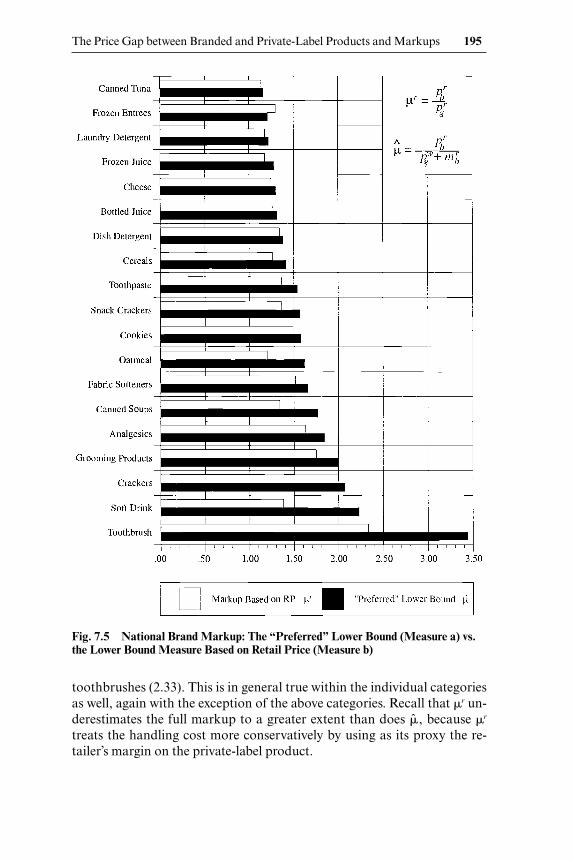
toothbrushes (2.33). This is in general true within the individual categoriesas well, again with the exception of the above categories. Recall that r un-derestimates the full markup to a greater extent than does , because r

treats the handling cost more conservatively by using as its proxy the re-tailer’s margin on the private-label product.


Fig. 7.5 National Brand Markup: The “Preferred” Lower Bound (Measure a) vs.the Lower Bound Measure Based on Retail Price (Measure b)

Summary

To further explore the relationship between our preferred lower-boundratio and the lower-bound ratios computed using the wholesale and the re-tail prices, we plot the three lower-bound series together in figure 7.6. As thefigure demonstrates, the lower-bound ratio calculated using the wholesaleprice usually exceeds our “preferred” lower bound, whereas the lower-bound ratio calculated using the retail price typically falls below the pre-


Fig. 7.6 Lower Bounds on the National Brand Manufacturers’ Markup Ratio: The“Preferred” Lower Bound (Measure a), the Lower Bound Based on Wholesale Price(Measure c), and the Lower Bound Based on Retail Price (Measure b)

ferred lower bound. The figure also indicates that the three lower-boundmeasures attain values that are closer to each other as the markups’ size de-creases.

7.5.2 Detailed Results for Some Selected Categories and Products

In tables 7A.1–7A.19, we report detailed tabulations of all five markupratios derived in section 7.2.3, for each national brand/private-label pair forall nineteen product categories included in our data set.

Among the nineteen categories, the toothbrush category (table 7A.1) at-tains the highest average value of our preferred lower-bound markup ratio,with a category average of 3.44. Within the category, four types of Cresttoothbrush (of different size and strength) attain a markup ratio in therange of 5.48–5.80, and two types of Reach toothbrush attain markup val-ues of 4.36 and 4.56. The results for the remaining products in this categorysuggest more moderate market power, with markup ratios in the range of1.56 for Johnson and Johnson waxed mint dental floss and 1.49 for the Pep-sodent toothbrush.

The manufacturers’ lower-bound markup ratios calculated using thewholesale prices attain even higher values. For example, for the four Crestand two Reach toothbrushes, w falls in the range of 13.00–19.84. Overall,the category average of these markup figures is 10.43. The reasons for thesevery high measured markup figures, unique to the toothbrush category, re-main a mystery.

The figures in the last two columns of table 7A.1 suggest that the retailer’smarkup on private-label products in this category far exceeds its markup ra-tio on the corresponding nationally branded product by nearly an order ofmagnitude. For example, for the highest markup brand, the Crest tooth-brush, the retailer’s markup ratio is only 1.14, whereas the markup ratio onthe corresponding private label is 7.03. Overall, the retailer’s averagemarkup ratio for nationally branded products in this category equals 1.37,whereas the average markup ratio for private-label products equals 4.87.

Finally, the lower-bound markup ratios calculated using the retail pricesare more moderate, although for the top four products the ratio still exceeds3.00, and for another two products it is close to 3.00. The category averagefor this ratio is 2.33.

For the remaining eighteen categories we find more moderate markupfigures. Nevertheless, in most categories they are quite substantial. For ex-ample, for the analgesics category, reported in table 7A.5, the average of ourpreferred lower-bound markup ratio is 1.84. Several products in this cate-gory have especially high markup ratios. For example, the preferred lowerbound on the markup ratio for children’s Anacin-3 tablets is 4.99 (column[1]). Four other products with especially high markup ratios are Panadolchildren’s tablets, with the lower-bound markup ratio of 3.91, followed by


Tylenol extra- strength caplets, with 2.53; Tylenol tablets (regular), with2.44; and Bayer children’s aspirin, with a markup ratio of 2.28.10

Turning to the manufacturers’ markup ratios calculated using the whole-sale prices (column [2]), we find that they are quantitatively very similar tothe values of , with the exception of children’s Anacin-3 tablets, with amanufacturer’s lower-bound markup ratio of 7.62, and Panadol children’stablets, with a manufacturer’s lower-bound markup ratio of 6.73. Further,as we move down the list from the highest preferred lower bound to the low-est, the discrepancy between the two ratios essentially disappears, as ex-pected. Overall, the lower-bound manufacturers’ markup ratios calculatedusing wholesale prices are high. For example, the figures in the table indi-cate that for seven of the twenty-four products in this category, the manu-facturers’ lower-bound markup ratio exceeds 2.00, and for another tenproducts the ratio exceeds 1.7. Only for two products, both Tylenol extra-strength tablets (different sizes), is w below 1.2. Overall, the average man-ufacturer’s lower-bound markup ratio for this category equals 2.01.

The figures in the third column of table 7A.5, which measure the lowerbound on the full markup using retail prices, are smaller than the first tworatios, as predicted by the inequalities derived in section 7.2.3. Still, themarkup ratios we obtain for the analgesics category are large. For example,of the twenty-four products, for three products—children’s Anacin-3 tab-lets, Panadol children’s tablets, and Tylenol extra-strength caplets—themarkup ratio calculated using only the retail prices exceeds 2.0; for tenother products the ratio exceeds 1.6, and for another eight products themarkup ratio exceeds 1.3. The average markup ratio using retail prices forthe analgesics category equals 1.63.

Finally, the retailer’s markup on the national brand systematically ex-ceeds its markup on the private label. For example, for twenty-three of thetwenty-four products (Bayer children’s aspirin being the only exception),the retailer’s markup on nationally branded products in this category is lessthan 1.15, with an overall average of only 1.04. In contrast, the markup ra-tio on the private label is substantially higher, averaging 1.25.

Next, consider the cereals category. According to table 7A.12, all of themarkup figures we find in this category are smaller than those we reportedfor the analgesics category. As the figures in the first column of the table sug-gest, here the preferred lower-bound markup ratio falls in the range 1.27–1.57, with an average of 1.41, again suggestive of very substantial marketpower. Total raisin bran attains the highest lower-bound value with 1.57,followed by Kellogg’s corn flakes, with 1.54, and Post raisin bran and Kel-logg’s Nut & Honey, each with a lower-bound markup ratio of 1.41.

The manufacturers’ markup figures reported in the second column of


10. Ernie Berndt noted that the extraordinarily high markups on children’s medicine mightpossibly be explained by parents’ risk aversion regarding their children’s health.

table 7A.12 are only slightly higher than the preferred lower-bound figures.For example, for Total raisin bran, the lower bound on the manufacturer’smarkup ratio equals 1.61, in comparison to the preferred lower bound of1.57. The manufacturers’ markup and the preferred markup figures areequally close for the remaining products of the category. Overall, cerealmanufacturers on average mark up their branded product prices to 1.43 oftheir marginal cost.

According to the third column of table 7A.12, the markup ratios we ob-tain using retail prices average 1.26 for the cereals category. Total raisinbran still attains the highest value with 1.46, and Kellogg’s corn flakes’markup ratio is a distant second with a value of 1.23. Finally, comparing theretailer’s markup ratio on branded products to its markup ratio on privatelabels, we again find that the latter, 1.19 on average, exceeds the former, 1.07on average.

It is instructive to compare our markup figures in this category to exist-ing econometric estimates. The category of breakfast cereals has been asubject of several recent studies, such as those by Hausman (1997) andNevo (2001). Nevo presents estimates of price-marginal cost margins underdifferent assumptions on market structure and finds that they range fromabout 1.3 to as high as 2.0, very much consistent with the lower-bound mea-sures reported here.

As a final example, consider the crackers category, in which we were ableto find ten matching pairs of national brand and private-label products. Ac-cording to table 7A.3, our preferred lower-bound markup figures are rela-tively high, with the highest ratio for Nabisco premium saltines (2.84), andthe lowest for Salerno graham crackers (1.34); the overall category averageis 2.07. For four branded products, two Nabisco Premium saltines (differ-ent sizes) and two Salerno saltines (also different sizes), the ratio exceeds2.00. Only for two products is the lower-bound markup ratio less than 1.40.

The manufacturers’ lower-bound markup ratios (second column of table7A.3) substantially exceed the preferred lower-bound figures. For example,the category average of the manufacturers’ lower-bound markup equals2.57, which is about 25 percent higher than the preferred lower bound.Further, for Nabisco Premium saltines, the manufacturer’s lower-boundmarkup ratio is 4.22, about 50 percent higher than the corresponding pre-ferred lower bound.

It turns out that in the crackers category we obtain especially highmarkup figures even if we consider the lower bound on the full markup ra-tio calculated using only the retail prices. For example, according to table7A.3 (column [3]), the category average of this markup ratio is 2.00, whichis the second highest (the toothbrush category being first) among all nine-teen categories included in our study. Individual product markup ratios cal-culated using the retail prices range from the highest ratio of 3.12 forNabisco premium saltines to 1.20 for Salerno graham crackers.


Finally, if we consider the retailer’s markup on the nationally brandedand private-label products, we find that, as before, the retailer’s markup onthe private label is systematically higher than its markup on the nationallybranded product, with an average of 1.50 in contrast to 1.15, a difference ofabout 20 percent.11

Next, consider some specific products that stand out in other categories.In the canned soup category (table 7A.6), the only nationally branded prod-uct with a preferred lower-bound markup ratio in excess of 2.00 is Camp-bell’s tomato soup, with a ratio of 2.61. The remaining products in this cat-egory attain a markup value of less than 2.00. In the cookies category (table7A.9), two brand-name products, Nutter Butter peanut butter and Cameocrème sandwich, attain a “preferred” lower-bound markup ratio of about2.70, and another ten products attain markup values exceeding 1.40. In thesnack cracker category (table 7A.10), Nabisco Ritz cracker attains the high-est preferred lower-bound markup ratio, 1.74, followed by Nabisco RitzBits, with a ratio of 1.58.

In the soft drinks category (table 7A.2), we find that Coca-Cola Classicand Pepsi cola attain preferred lower-bound markup values of 3.83 and2.36, respectively. Other branded products with particularly high lower-bound markup ratios in the soft drink category are Schweppes ginger ale,with 3.52; Snapple strawberry and Snapple pink lemonade, with 2.88 and2.47, respectively; Diet Pepsi, with 2.28; and Seagrams ginger ale, with 2.18.Diet Coke attains a more moderate lower-bound markup ratio of 1.69.

Finally, the nationally branded products attaining the highest preferredlower-bound markup ratios in the remaining categories include Motts ap-ple juice in the bottled juice category, Minute Maid pink lemonade in thefrozen juice category, Crest Regular in the toothpaste category, Kraft softPhilly cream cheese in the cheese category, Dawn lemon in the dish deter-gent category, L.C. Baked cheese ravioli in the frozen entrees category,Bounce single scented in the fabric softener category, Trac II Plus cart 10 inthe grooming products category, ultra Ivory Snow in the laundry detergentcategory, quick Quaker oats in the oatmeal category, and Chicken of the Sealite tuna in water in the canned tuna category.

7.6 The Role of the Materials Share

It might be worthwhile to hypothesize as to the determinants of cross-category and within-category variation in the magnitude of markup ratios.Consider first the within-category variation. In most categories, we find


11. Slade (1998) assumes a 20 percent retail markup for saltine crackers in her study of priceadjustment costs at several Pennsylvania grocery stores. This is equivalent to a retailer’smarkup ratio of 1.20. The average retailer’s markup ratio on the nationally branded productwe report is 1.15, with the interquartile range of (1.12–1.17) indeed very close to what Slade as-sumes.

that more heavily branded and well-known products achieve higher mark-ups. For example, Kellogg’s corn flakes, Nabisco Premium saltine crackers,Crest toothpaste, Coca-Cola Classic, Motts apple juice, Nutter Butterpeanut butter, Nabisco Ritz crackers, Kraft cream cheese, Dawn lemon dishdetergent, Bounce single scented fabric softener, and so on, which have thehighest markups within respective categories, all are heavily advertised andwidely recognized nationally branded products.

Perhaps a more interesting issue is the variation in markup ratios acrossproduct categories. Basu and Fernald (1997) and Rotemberg and Woodford(1996) provide the following formula linking the gross output markups thatare the focus of this paper to the value added markups, via products mate-rial share:

v � �

1

(1

�

�

s

s

)�,

where v denotes the markup on real value added, s denotes the intermedi-ate inputs share in total revenue, and denotes the gross output markup.The formula implies that if the value added markup is to be finite, the grossoutput markup must not exceed 1/s.

Nevo (2001), using data from the Annual Survey of Manufacturers overthe period 1988–92, provides materials share figures for ready-to-eat cere-als (SIC [Standard Industrial Classification] 2043) and for the food indus-try overall (SIC 20). For cereals, he reports a materials share of 26.5 per-cent, which from the above formula implies that the gross output markupshould not exceed 1/0.265 � 3.77. Indeed, according to our findings (see fig-ure 7.1), the preferred lower-bound markup ratio for the cereals categoryequals 1.41, well below the upper bound imposed by the above formula.

For the entire food industry, Nevo reports a materials share of 63.4 per-cent. This imposes an upper bound of 1.58 on the gross output markup ra-tio. Twelve of the nineteen categories we study would be classified as food.These are soft drinks, crackers, canned soups, oatmeal, cookies, snackcrackers, cereals, bottled juice, cheese, frozen juice, frozen entrees, andcanned tuna. Of these twelve categories, the numerical values of the pre-ferred markup ratios for the last eight categories fall below 1.58. For two ad-ditional categories (oatmeal and canned soups), the markup ratio is onlyslightly higher than 1.58. For only two categories (crackers and soft drinks)does the markup ratio substantially exceed 1.58. This suggests that materi-als share in these two categories must be smaller than 26.5 percent, whichseems reasonable. Moreover, the interquartile ranges we report indicatethat the great majority of the products in each one of the twelve categoriessatisfy this constraint.

Finally, without having actual data on the cost shares of intermediate in-puts used by manufacturers of individual food categories, we strongly sus-pect that the products with the lowest markup ratios, such as canned tuna,


frozen entrees, cheese, frozen juice, and bottled juice, also have the highestshare of materials.12

7.7 Concluding Remarks

In this paper we study the size of markups for nationally branded prod-ucts sold in a large U.S. retail supermarket chain. Our approach, which wehope will serve as a complement to more structural econometric ap-proaches, treats the wholesale price of a comparable private-label productas an upper bound on the marginal costs faced by the brand manufacturer.Using scanner data from a large Midwestern chain, we have computed var-ious upper- and lower-bound markup ratios for over 230 products in nine-teen categories. We found that markup ratios measured this way range from3.44 for toothbrushes and 2.23 for soft drinks to about 1.15–1.20 for cannedtuna and frozen entrees, with the majority of categories falling in the range1.40–2.10. Lower bounds on manufacturers’ markups are even higher.Thus, the data indicate that markups on nationally branded products soldin U.S. supermarkets are large.

Our approach offers several benefits. Because it involves only a simplecomputation (once the data have been assembled), the method permits cal-culation of markups for a large variety of products. It is transparent andintuitive, and it offers a benchmark comparison for more structural ap-proaches.

Particularly in light of the importance of markups in recent macroeco-nomic discourse, one might ask whether the finding of high markups forheavily advertised differentiated products generalizes to the economy atlarge. In this direction, it is worth noting that many “commodity” productssuch as automotive parts, personal computers and their components, andmany other producers’ goods come in both branded and nonbranded(OEM or Original Equipment Manufacturer) versions, and that the pricegap for those products is comparable to that for the supermarket goods wehave studied. This is also true for other consumer goods sold outside the su-permarket industry, home and office supply products being one example.

Appendix

In this appendix we present detailed results for each pair of national brandand private-label products, for each of the nineteen product categories in-


12. We are grateful to Susanto Basu for calling our attention to the above formula and itsimplications.

cluded in our data set. The results are reported in separate tables, tables7A.1 through 7A.19, by categories.

In these tables, columns (1)–(5) correspond to the five markup measureswe report in the paper, as follows:

1. Column (1) corresponds to the markup measure (a), , which is our“preferred” lower bound on the full markup.

2. Column (2) corresponds to the markup measure (c), w, which pro-vides a lower bound on manufacturers’ markup by using wholesale prices.

3. Column (3) corresponds to the markup measure (b), r, which pro-vides a lower bound on the full markup by using retail prices.

4. Column (4) corresponds to the markup measure (d), b, which is theretailer’s markup on the nationally branded product.

5. Column (5) corresponds to the markup measure (e), g, which mea-sures the retailer’s markup on private label product.

In each table, the figures in parentheses indicate the interquartile range.The sample size numbers, which are listed in the last column of each table,report the number of weekly time series observations of price and cost dataused in calculating the various markup measures for the corresponding na-tional brand/private-label product pair. See text for more details.


Tab

le 7

A.1

Toot

hbru

sh

Ful

l Mar

kup:

Man

ufac

ture

r’s M

arku

p:L

ower

Bou

nd fo

rR

etai

ler’s

Ret

aile

r’s“P

refe

rred

”L

ower

Bou

nd b

ased

Ful

l Mar

kup

Bas

edM

arku

p on

Mar

kup

onL

ower

Bou

ndon

Who

lesa

le P

rice

on R

etai

l Pri

ceN

atio

nal B

rand

Pri

vate

Lab

elSa

mpl

eP

rodu

ct P

air

()

(w)

(r )

(b)

(g)

Size

Cre

st to

othb

rush

#5

soft

5.80

(4.5

5, 6

.35)

19.8

4 (8

.64,

41.

23)

3.33

(2.8

8, 3

.75)

1.14

(1.1

2, 1

.16)

7.03

(3.2

6, 1

3.17

)17

0C

rest

toot

hbru

sh #

1 m

ediu

m s

tron

g5.

75 (4

.68,

6.4

0)23

.70

(8.6

4, 4

1.23

)3.

34 (2

.88,

3.7

5)1.

14 (1

.12,

1.1

6)8.

01 (3

.26,

13.

17)

170

Cre

st to

othb

rush

#2

med

ium

str

ong

5.57

(4.5

5, 6

.35)

19.2

6 (8

.64,

39.

86)

3.31

(2.8

8, 3

.75)

1.14

(1.1

2, 1

.16)

6.65

(3.2

6, 1

3.17

)17

0C

rest

toot

hbru

sh #

6 so

ft5.

48 (4

.55,

6.3

5)16

.20

(8.6

4, 3

8.91

)3.

28 (2

.88,

3.7

5)1.

14 (1

.12,

1.1

6)5.

78 (3

.26,

13.

17)

170

Rea

ch b

etw

een

soft

4.56

(3.7

9, 5

.19)

17.9

7 (8

.27,

34.

60)

2.92

(2.5

9, 3

.32)

1.21

(1.2

0, 1

.22)

7.70

(3.2

6, 1

3.17

)17

0R

each

bet

wee

n m

ediu

m4.

36 (3

.79,

5.1

3)13

.00

(8.9

6, 2

9.79

)2.

92 (2

.52,

3.3

2)1.

21 (1

.20,

1.2

2)5.

77 (3

.26,

13.

17)

170

J&J

floss

wax

ed m

int

1.56

(1.5

4, 1

.63)

2.05

(2.0

2, 2

.24)

1.54

(1.5

0, 1

.75)

1.41

(1.4

1, 1

.45)

1.90

(1.8

7, 1

.94)

164

J&J

floss

wax

ed r

egul

ar1.

55 (1

.54,

1.6

3)2.

05 (2

.02,

2.2

5)1.

52 (1

.49,

1.7

1)1.

42 (1

.41,

1.4

5)1.

92 (1

.87,

1.9

4)16

3J&

J flo

ss u

nwax

ed r

egul

ar1.

55 (1

.53,

1.6

4)2.

04 (2

.00,

2.2

6)1.

51 (1

.49,

1.7

1)1.

42 (1

.41,

1.4

5)1.

93 (1

.90,

1.9

4)16

4P

epso

dent

toot

hbru

sh m

ediu

m1.

50 (1

.37,

1.7

3)3.

33 (1

.96,

7.3

9)1.

17 (1

.00,

1.4

3)2.

04 (1

.97,

2.0

2)5.

65 (3

.26,

13.

17)

170

Pep

sode

nt to

othb

rush

sof

t per

fect

1.49

(1.3

4, 1

.76)

3.16

(1.9

3, 7

.85)

1.16

(1.0

0, 1

.43)

1.95

(1.9

5, 2

.00)

5.52

(2.9

2, 1

3.17

)17

0W

eigh

ted

aver

age

3.44

(1.5

5, 5

.57)

10.4

3 (2

.05,

19.

26)

2.33

(1.5

1, 3

.31)

1.37

(1.1

4, 1

.42)

4.87

(1.9

3, 7

.03)

Not

es:C

olum

n on

e co

rres

pond

s to

mar

kup

mea

sure

(a),

col

umn

two

to m

arku

p m

easu

re (c

), c

olum

n th

ree

to m

arku

p m

easu

re (b

), c

olum

n fo

ur to

mar

kup

mea

-su

re (d

), a

nd c

olum

n fiv

e—to

mar

kup

mea

sure

Fig

ures

in th

e pa

rent

hese

s in

dica

te th

e in

ter-

quar

tile

ran

ge. S

ee te

xt fo

r de

tails

.

Tab

le 7

A.2

Sof

t Dri

nk

Ful

l Mar

kup:

Man

ufac

ture

r’s M

arku

p:L

ower

Bou

nd fo

rR

etai

ler’s

Ret

aile

r’s“P

refe

rred

”L

ower

Bou

nd b

ased

Ful

l Mar

kup

Bas

edM

arku

p on

Mar

kup

onL

ower

Bou

ndon

Who

lesa

le P

rice

on R

etai

l Pri

ceN

atio

nal B

rand

Pri

vate

Lab

elSa

mpl

eP

rodu

ct P

air

()

(w)

(r )

(b)

(g)

Size

Coc

a-C

ola

clas

sic

3.83

(1.8

4, 2

.55)

2.35

(2.1

0, 3

.07)

1.38

(1.2

0, 1

.89)

1.15

(1.0

3, 1

.24)

1.91

(1.4

1, 2

.10)

389

Schw

eppe

s gi

nger

ale

3.52

(1.0

7, 2

.14)

2.17

(1.6

9, 2

.96)

1.30

(1.1

1, 1

.71)

1.15

(0.9

6, 1

.26)

1.74

(1.4

1, 2

.05)

390

Snap

ple

stra

wbe

rry

kiw

i2.

88 (1

.49,

1.7

5)2.

36 (2

.13,

2.7

2)1.

02 (1

.22,

1.5

1)1.

20 (1

.47,

1.6

8)2.

88 (2

.55,

3.0

5)10

8Sn

appl

e pi

nk le

mon

ade

2.47

(1.4

9, 1

.75)

2.26

(2.1

3, 2

.74)

1.06

(1.2

2, 1

.51)

1.27

(1.4

7, 1

.68)

2.83

(2.5

5, 3

.05)

122

Pep

si c

ola

n/r

2.36

(1.9

0, 2

.73)

2.23

(2.1

9, 3

.21)

1.38

(1.2

2, 1

.89)

1.18

(1.0

3, 1

.18)

1.83

(1.4

1, 2

.10)

390

Pep

si d

iet n

/r2.

28 (1

.86,

2.6

9)2.

25 (2

.15,

3.1

4)1.

41 (1

.22,

1.9

0)1.

14 (1

.03,

1.1

8)1.

78 (1

.40,

2.0

9)39

0Se

agra

ms

ging

er a

le 1

2.18

(1.8

1, 2

.48)

2.47

(2.4

8, 2

.91)

1.37

(1.2

5, 1

.68)

1.21

(1.0

7, 1

.39)

2.13

(2.0

3, 2

.30)

75P

epsi

col

a2.

07 (1

.70,

2.2

3)2.

07 (1

.87,

2.2

5)1.

53 (1

.42,

1.7

1)1.

06 (1

.02,

1.1

5)1.

42 (1

.38,

1.4

6)22

2Sc

hwep

pes

lime

selt

zer

2.06

(1.4

7, 2

.61)

1.97

(1.4

8, 2

.55)

1.23

(1.2

0, 1

.20)

1.20

(1.0

1, 1

.37)

1.88

(1.6

3, 2

.15)

36Se

agra

ms

toni

c 1

liter

2.05

(1.7

8, 1

.89)

2.52

(2.4

3, 2

.70)

1.44

(1.3

2, 1

.59)

1.26

(1.3

2, 1

.35)

2.20

(2.1

3, 2

.28)

125

Bar

q’s

root

bee

r1.

95 (1

.63,

2.2

6)2.

00 (1

.86,

2.4

8)1.

39 (1

.12,

1.8

0)1.

26 (1

.03,

1.3

0)1.

76 (1

.45,

2.0

4)36

4Sc

hwep

pes

toni

c n/

r1.

94 (1

.36,

2.2

5)2.

28 (1

.75,

2.7

3)1.

36 (1

.19,

1.5

1)1.

37 (1

.06,

1.4

7)2.

09 (1

.87,

2.3

9)38

8Sc

hwep

pes

diet

toni

c1.

93 (1

.36,

2.2

3)2.

29 (1

.75,

2.7

3)1.

35 (1

.19,

1.5

1)1.

37 (1

.06,

1.4

7)2.

10 (1

.87,

2.3

9)38

8R

oyal

Cro

wn

cola

1.89

(1.4

6, 2

.48)

1.88

(1.7

5, 2

.85)

1.19

(1.1

1, 1

.61)

1.32

(1.0

3, 1

.26)

1.75

(1.4

0, 2

.05)

389

A&

W ro

ot b

eer

regu

lar

1.86

(1.3

0, 2

.13)

1.78

(1.4

9, 2

.54)

1.16

(1.0

2, 1

.51)

1.14

(1.0

2, 1

.26)

1.68

(1.4

0, 2

.02)

389

Min

ute

Mai

d fr

uit p

unch

1.80

(1.6

6, 1

.97)

2.33

(2.0

1, 2

.62)

1.48

(1.2

5, 1

.75)

1.18

(1.1

5, 1

.30)

1.97

(1.7

9, 2

.32)

86A

&W

root

bee

r1.

79 (1

.73,

2.0

1)1.

80 (1

.77,

2.0

7)1.

68 (1

.60,

1.9

8)1.

01 (0

.99,

1.0

7)1.

09 (1

.08,

1.1

2)25

3N

ew Y

ork

selt

zer

cola

1.77

(1.1

6, 2

.04)

2.66

(1.2

3, 3

.26)

1.70

(1.1

9, 1

.95)

1.35

(1.3

6, 1

.36)

2.03

(1.4

0, 2

.34)

34Sn

appl

e ki

wi s

traw

berr

y s

1.75

(1.4

0, 1

.74)

2.38

(2.1

2, 2

.74)

1.29

(1.2

2, 1

.37)

1.47

(1.4

8, 1

.74)

2.93

(2.8

0, 3

.05)

36Su

nkis

t ora

nge

1.75

(1.1

7, 2

.17)

1.46

(1.4

0, 2

.46)

1.10

(1.0

0, 1

.48)

1.64

(1.0

3, 1

.32)

1.79

(1.4

5, 2

.05)

390

Schw

eppe

s gi

nger

ale

1.73

(1.2

9, 2

.10)

2.06

(1.6

0, 2

.67)

1.31

(1.1

4, 1

.47)

1.49

(1.2

1, 1

.68)

2.06

(1.8

0, 2

.43)

340

Can

ada

Dry

gin

ger

ale

1.72

(1.3

4, 1

.93)

2.36

(1.7

6, 2

.50)

1.48

(1.2

7, 1

.52)

1.47

(1.3

0, 1

.55)

2.09

(1.8

1, 2

.43)

305

A&

W ro

ot b

eer

suga

r fr

ee1.

70 (1

.25,

2.0

8)1.

72 (1

.44,

2.5

4)1.

18 (1

.06,

1.5

1)1.

19 (1

.02,

1.2

6)1.

67 (1

.41,

2.0

2)38

9D

iet C

oke

1.69

(1.8

4, 2

.53)

2.25

(2.1

2, 3

.03)

1.42

(1.2

1, 1

.89)

1.14

(1.0

3, 1

.24)

1.80

(1.4

0, 2

.09)

389

(con

tinu

ed)

Tab

le 7

A.2

(con

tinu

ed)

Ful

l Mar

kup:

Man

ufac

ture

r’s M

arku

p:L

ower

Bou

nd fo

rR

etai

ler’s

Ret

aile

r’s“P

refe

rred

”L

ower

Bou

nd b

ased

Ful

l Mar

kup

Bas

edM

arku

p on

Mar

kup

onL

ower

Bou

ndon

Who

lesa

le P

rice

on R

etai

l Pri

ceN

atio

nal B

rand

Pri

vate

Lab

elSa

mpl

eP

rodu

ct P

air

()

(w)

(r )

(b)

(g)

Size

Can

ada

Dry

toni

c w

ater

1.69

(1.3

9, 1

.90)

2.42

(1.8

0, 2

.55)

1.48

(1.2

9, 1

.59)

1.47

(1.3

0, 1

.50)

2.11

(1.9

1, 2

.39)

355

Min

ute

Mai

d or

ange

1.69

(1.3

8, 2

.12)

1.72

(1.4

5, 2

.11)

1.67

(1.5

0, 2

.01)

1.08

(1.0

1, 1

.12)

1.09

(1.0

8, 1

.13)

52O

cean

Spr

ay k

iwi s

traw

berr

y1.

67 (1

.60,

1.7

9)2.

66 (2

.49,

2.9

6)1.

54 (1

.48,

1.6

8)1.

56 (1

.52,

1.6

4)2.

74 (2

.22,

3.0

5)73

Cry

stal

Lig

ht k

iwi s

traw

berr

y1.

65 (1

.55,

1.7

5)2.

54 (2

.36,

2.8

0)1.

39 (1

.34,

1.5

9)1.

54 (1

.47,

1.6

5)2.

89 (2

.55,

3.0

5)81

Pep

si c

ola

cans

1.63

(1.6

6, 2

.06)

1.65

(1.6

4, 2

.09)

1.58

(1.5

0, 2

.01)

1.05

(1.0

0, 1

.04)

1.09

(1.0

7, 1

.10)

202

Fru

itop

ia p

ink

lem

onad

e1.

61 (1

.58,

1.6

5)2.

43 (2

.45,

2.5

4)1.

42 (1

.31,

1.5

1)1.

56 (1

.51,

1.6

5)2.

81 (2

.80,

3.0

5)10

2Su

nkis

t ora

nge

1.58

(1.5

9, 1

.79)

1.62

(1.6

6, 1

.85)

1.53

(1.6

0, 1

.81)

1.03

(1.0

3, 1

.06)

1.10

(1.0

8, 1

.12)

254

Bar

q’s

diet

root

bee

r1.

56 (1

.71,

2.2

9)2.

12 (1

.92,

2.4

0)1.

27 (1

.03,

1.4

0)1.

06 (1

.02,

1.1

9)1.

86 (1

.57,

2.1

2)62

Roy

al C

row

n co

la1.

56 (1

.54,

1.8

7)1.

65 (1

.67,

2.0

8)1.

30 (1

.31,

1.7

1)1.

12 (1

.10,

1.1

8)1.

42 (1

.38,

1.4

6)22

2M

inut

e M

aid

oran

ge1.

55 (1

.47,

1.7

2)1.

81 (1

.62,

2.0

3)1.

23 (1

.11,

1.3

4)1.

19 (1

.14,

1.2

6)1.

76 (1

.40,

2.0

2)13

7Se

agra

ms

ging

er a

le1.

44 (1

.46,

1.9

6)1.

99 (1

.74,

2.3

9)1.

37 (1

.12,

1.7

9)1.

33 (1

.09,

1.4

0)1.

88 (1

.57,

2.1

2)17

7B

arq’

s ro

ot b

eer

1.40

(1.7

4, 2

.38)

2.20

(1.9

9, 2

.49)

1.22

(1.0

3, 1

.40)

1.06

(1.0

2, 1

.21)

1.97

(1.7

9, 2

.12)

56B

arq’

s ro

ot b

eer

1.36

(1.3

2, 1

.49)

1.48

(1.4

4, 1

.64)

1.01

(0.9

6, 1

.12)

1.19

(1.1

4, 1

.27)

1.75

(1.4

1, 2

.01)

31Se

agra

m’s

lem

on li

me

1.04

(1.4

3, 1

.65)

1.75

(1.6

7, 2

.00)

1.31

(1.1

2, 1

.20)

1.29

(1.1

8, 1

.39)

1.81

(1.6

4, 2

.12)

50W

eigh

ted

aver

age

2.23

(1.5

6, 2

.13)

2.09

(1.7

2, 2

.29)

1.38

(1.1

9, 1

.48)

1.18

(1.1

4, 1

.37)

1.76

(1.7

0, 1

.99)

Not

es:S

ee ta

ble

7A.1

.

Tab

le 7

A.3

Cra

cker

s

Ful

l Mar

kup:

Man

ufac

ture

r’s M

arku

p:L

ower

Bou

nd fo

rR

etai

ler’s

Ret

aile

r’s“P

refe

rred

”L

ower

Bou

nd B

ased

Ful

l Mar

kup

Bas

edM

arku

p on

Mar

kup

onL

ower

Bou

ndon

Who

lesa

le P

rice

on R

etai

l Pri

ceN

atio

nal B

rand

Pri

vate

Lab

elSa

mpl

eP

rodu

ct P

air

()

(w)

(r )

(b)

(g)

Size

Nab

isco

pre

miu

m s

alti

nes

2.84

(2.6

2, 3

.12)

4.22

(3.7

1, 4

.51)

3.12

(2.2

7, 3

.86)

1.17

(1.1

4, 1

.18)

1.63

(1.3

6, 1

.81)

125

Nab

isco

pre

miu

m s

alti

nes

2.30

(2.1

4, 2

.43)

2.75

(2.5

0, 3

.08)

2.32

(2.1

4, 2

.61)

1.15

(1.1

1, 1

.17)

1.35

(1.2

0, 1

.57)

82Sa

lern

o sa

ltin

es2.

11 (2

.05,

2.2

3)

2.47

(2.3

4, 2

.68)

2.11

(1.8

9, 2

.40)

1.13

(1.1

0, 1

.16)

1.34

(1.2

0, 1

.57)

82Sa

lern

o sa

ltin

es2.

03 (1

.72,

2.4

2)2.

97 (2

.47,

3.5

1)2.

39 (1

.90,

2.9

8)1.

28 (1

.17,

1.3

6)1.

63 (1

.36,

1.8

1)12

5N

abis

co p

rem

ium

sal

tine

s1.

83 (1

.60,

2.0

4)2.

08 (1

.77,

2.3

9)1.

44 (1

.20,

1.6

5)1.

16 (1

.13,

1.1

8)1.

68 (1

.58,

1.7

1)37

2H

oney

Mai

d gr

aham

s1.

67 (1

.55,

1.6

9)1.

81 (1

.65,

1.8

2)1.

45 (1

.37,

1.4

2)1.

11 (1

.10,

1.1

2)1.

38 (1

.32,

1.4

2)90

Kee

bler

gra

ham

cra

cker

s1.

58 (1

.48,

1.6

9)1.

70 (1

.58,

1.8

3)1.

39 (1

.27,

1.5

0)1.

12 (1

.10,

1.1

3)1.

37 (1

.32,

1.4

2)38

0N

abis

co g

raha

m c

rack

ers

1.52

(1.4

3, 1

.64)

1.63

(1.5

0, 1

.76)

1.31

(1.2

2, 1

.41)

1.10

(1.1

0, 1

.12)

1.37

(1.3

2, 1

.42)

380

Sale

rno

salt

ines

1.37

(1.2

4, 1

.56)

1.52

(1.3

4, 1

.77)

1.14

(1.0

0, 1

.30)

1.27

(1.1

7, 1

.36)

1.67

(1.5

9, 1

.71)

372

Sale

rno

grah

am c

rack

ers

1.34

(1.2

6, 1

.41)

1.42

(1.3

2, 1

.50)

1.20

(1.1

2, 1

.23)

1.15

(1.1

4, 1

.18)

1.37

(1.3

2, 1

.41)

380

Wei

ghte

d av

erag

e2.

07 (1

.52,

2.1

1)2.

57 (1

.63,

2.7

5)2.

00 (1

.31,

2.3

2)1.

15 (1

.12,

1.1

7)1.

50 (1

.37,

1.6

3)

Not

es:S

ee ta

ble

7A.1

.

Tab

le 7

A.4

Gro

omin

g P

rodu

cts

Ful

l Mar

kup:

Man

ufac

ture

r’s M

arku

p:L

ower

Bou

nd fo

rR

etai

ler’s

Ret

aile

r’s“P

refe

rred

”L

ower

Bou

nd B

ased

Ful

l Mar

kup

Bas

edM

arku

p on

Mar

kup

onL

ower

Bou

ndon

Who

lesa

le P

rice

on R

etai

l Pri

ceN

atio

nal B

rand

Pri

vate

Lab

elSa

mpl

eP

rodu

ct P

air

()

(w)

(r )

(b)

(g)

Size

Tra

c II

plu

s ca

rtri

dge

102.

30 (2

.13,

2.4

5)2.

43 (2

.22,

2.6

0)2.

04 (1

.88,

2.1

6)1.

04 (1

.04,

1.0

4)1.

24 (1

.24,

1.2

6)80

Slim

twin

dis

posa

bl2.

29 (1

.78,

2.5

7)2.

86 (2

.47,

3.1

8)1.

77 (1

.68,

1.8

9)1.

18 (1

.12,

1.1

7)1.

89 (1

.91,

1.9

3)21

1~S

lim tw

in c

artr

idge

1.96

(1.9

4, 1

.97)

2.04

(2.0

2, 2

.05)

1.70

(1.6

9, 1

.72)

1.04

(1.0

4, 1

.04)

1.24

(1.2

4, 1

.25)

73G

ood

New

s pi

vot p

lus

1.63

(1.3

5, 2

.02)

1.77

(1.4

1, 2

.27)

1.55

(1.2

3, 1

.95)

1.09

(1.0

9, 1

.11)

1.25

(1.2

4, 1

.27)

100

Goo

d N

ews

pivo

t plu

s1.

47 (1

.30,

1.4

2)1.

55 (1

.33,

1.5

0)1.

35 (1

.17,

1.3

8)1.

08 (1

.07,

1.1

0)1.

24 (1

.24,

1.2

4)11

5W

eigh

ted

aver

age

2.00

(1.6

3, 2

.29)

2.17

(1.7

7, 2

.43)

1.75

(1.5

5, 1

.77)

1.07

(1.0

4, 1

.09)

1.33

(1.2

4, 1

.25)

Not

es:S

ee ta

ble

7A.1

. The

sym

bol “

~” is

an

inte

rnal

cod

e us

ed b

y D

omin

ick’

s to

iden

tify

dis

cont

inue

d pr

oduc

ts.

Tab

le 7

A.5

Ana

lges

ics

Ful

l Mar

kup:

Man

ufac

ture

r’s M

arku

p:L

ower

Bou

nd fo

rR

etai

ler’s

Ret

aile

r’s“P

refe

rred

”L

ower

Bou

nd B

ased

Ful

l Mar

kup

Bas

edM

arku

p on

Mar

kup

onL

ower

Bou

ndon

Who

lesa

le P

rice

on R

etai

l Pri

ceN

atio

nal B

rand

Pri

vate

Lab

elSa

mpl

eP

rodu

ct P

air

()

(w)

(r )

(b)

(g)

Size

Ana

cin-

3 ch

ildre

n’s

tabl

ets

4.99

(4.9

0, 5

.03)

7.62

(7.4

1, 7

.84)

3.77

(3.6

5, 3

.94)

1.09

(1.0

8, 1

.10)

2.20

(2.1

8, 2

.20)

40P

anad

ol c

hild

ren’

s ta

blet

s3.

91 (3

.84,

3.9

3)6.

73 (6

.75,

7.2

5)3.

51 (3

.51,

3.7

8)1.

14 (1

.14,

1.1

6)2.

20 (2

.18,

2.2

0)

43

Tyle

nol e

xtra

str

engt

h ca

plet

2.53

(2.2

4, 2

.76)

2.81

(2.3

8, 3

.08)

2.23

(1.9

1, 2

.46)

1.06

(1.0

5, 1

.06)

1.33

(1.2

9, 1

.35)

392

Tyle

nol t

able

ts r

egul

ar2.

44 (1

.66,

3.2

9)2.

50 (1

.68,

3.3

7)1.

92 (1

.40,

2.4

2)1.

02 (1

.01,

1.0

2)1.

30 (1

.23,

1.3

8)39

2B

ayer

chi

ldre

n’s

aspi

rin

2.28

(2.1

6, 2

.36)

3.23

(3.0

4, 3

.36)

1.81

(1.7

2, 1

.91)

1.23

(1.2

2, 1

.25)

2.19

(2.1

8, 2

.20)

43Ty

leno

l inf

ant d

rops

1.94

(1.8

7, 1

.91)

2.09

(2.0

1, 2

.05)

1.71

(1.6

7, 1

.68)

1.07

(1.0

7, 1

.08)

1.31

(1.3

0, 1

.31)

114

~Exc

edri

n IB

cap

lets

1.91

(1.7

8, 1

.98)

2.04

(1.8

6, 2

.14)

1.78

(1.6

3, 1

.89)

1.07

(1.0

6, 1

.07)

1.22

(1.2

2, 1

.23)

89~E

xced

rin

IB ta

blet

s 50

1.86

(1.6

9, 1

.97)

1.97

(1.7

7, 2

.11)

1.68

(1.5

4, 1

.84)

1.06

(1.0

6, 1

.07)

1.24

(1.2

2, 1

.26)

67A

dvil

1.84

(1.6

8, 1

.91)

1.91

(1.7

3, 1

.98)

1.62

(1.4

9, 1

.69)

1.04

(1.0

3, 1

.05)

1.22

(1.2

1, 1

.24)

349

Tyle

nol e

xtra

str

engt

h ge

lcap

s1.

82 (1

.55,

2.0

9)1.

86 (1

.57,

2.1

3)1.

69 (1

.45,

1.9

3)1.

02 (1

.02,

1.0

3)1.

12 (1

.11,

1.1

3)36

5M

otri

n IB

gel

caps

1.79

(1.6

8, 1

.82)

1.86

(1.7

4, 1

.88)

1.60

(1.5

3, 1

.61)

1.04

(1.0

4, 1

.05)

1.21

(1.2

0, 1

.21)

134

Ale

ve c

aple

ts1.

79 (1

.67,

1.8

5)1.

86 (1

.72,

1.9

4)1.

61 (1

.50,

1.6

9)1.

05 (1

.04,

1.0

5)1.

21 (1

.20,

1.2

2)14

5~E

xced

rin

IB ta

blet

s 50

1.79

(1.6

5, 1

.95)

1.89

(1.7

2, 2

.08)

1.63

(1.4

7, 1

.80)

1.06

(1.0

6, 1

.08)

1.24

(1.2

2, 1

.26)

109

Tyle

nol e

xtra

str

engt

h ta

blet

s1.

79 (1

.53,

1.8

5)1.

81 (1

.55,

1.8

7)1.

56 (1

.37,

1.6

0)1.

01 (1

.01,

1.0

2)1.

18 (1

.12,

1.2

1)34

9A

dvil

1.69

(1.5

7, 1

.85)

1.72

(1.5

8, 1

.90)

1.56

(1.4

3, 1

.72)

1.02

(1.0

1, 1

.03)

1.13

(1.1

2, 1

.13)

365

Chi

ldre

n’s

chew

able

frui

t Tyl

enol

1.67

(1.6

0, 1

.79)

1.83

(1.7

2, 2

.00)

1.40

(1.3

2, 1

.53)

1.13

(1.1

2, 1

.14)

1.47

(1.4

4, 1

.49)

71C

hild

ren’

s ch

ewab

le g

rape

Tyl

enol

1.66

(1.5

4, 1

.79)

1.82

(1.6

6, 2

.00)

1.39

(1.3

0, 1

.53)

1.13

(1.1

2, 1

.14)

1.47

(1.4

4, 1

.49)

68A

dvil

1.59

(1.4

1, 1

.69)

1.61

(1.4

2, 1

.71)

1.46

(1.2

9, 1

.55)

1.02

(1.0

2, 1

.02)

1.12

(1.1

2, 1

.13)

39M

otri

n IB

cap

lets

1.53

(1.4

7, 1

.55)

1.55

(1.4

8, 1

.57)

1.42

(1.3

5, 1

.43)

1.02

(1.0

2, 1

.03)

1.12

(1.1

2, 1

.12)

248

~Exc

edri

n IB

cap

lets

1.46

(1.2

8, 1

.51)

1.48

(1.2

9, 1

.54)

1.36

(1.1

9, 1

.42)

1.03

(1.0

3, 1

.04)

1.13

(1.1

2, 1

.13)

75~E

xced

rin

IB ta

blet

s 10

01.

44 (1

.38,

1.4

9)1.

47 (1

.40,

1.5

2)1.

35 (1

.29,

1.3

9)1.

03 (1

.03,

1.0

4)1.

13 (1

.13,

1.1

3)95

Adv

il ca

plet

s1.

41 (1

.37,

1.4

7)1.

42 (1

.37,

1.4

9)1.

28 (1

.24,

1.3

5)1.

02 (1

.01,

1.0

2)1.

12 (1

.12,

1.1

2)24

5Ty

leno

l ext

ra s

tren

gth

tabl

ets

1.18

(1.1

2, 1

.19)

1.18

(1.1

2, 1

.20)

1.02

(0.9

8, 1

.04)

1.03

(1.0

3, 1

.03)

1.19

(1.1

7, 1

.20)

239

Tyle

nol e

xtra

str

engt

h ta

blet

s1.

17 (1

.11,

1.1

9)1.

18 (1

.12,

1.2

0)1.

02 (0

.98,

1.0

4)1.

03 (1

.03,

1.0

3)1.

19 (1

.17,

1.1

9)23

8W

eigh

ted

aver

age

1.84

(1.5

6, 1

.92)

2.01

(1.5

8, 2

.06)

1.63

(1.4

0, 1

.75)

1.04

(1.0

2, 1

.07)

1.25

(1.1

3, 1

.32)

Not

es:S

ee ta

ble

7A.1

. The

sym

bol “

~” is

an

inte

rnal

cod

e us

ed b

y D

omin

ick’

s to

iden

tify

dis

cont

inue

d pr

oduc

ts.

Tab

le 7

A.6

Can

ned

Sou

p

Ful

l Mar

kup:

Man

ufac

ture

r’s M

arku

p:L

ower

Bou

nd fo

rR

etai

ler’s

Ret

aile

r’s“P

refe

rred

”L

ower

Bou

nd B

ased

Ful

l Mar

kup

Bas

edM

arku

p on

Mar

kup

onL

ower

Bou

ndon

Who

lesa

le P

rice

on R

etai

l Pri

ceN

atio

nal B

rand

Pri

vate

Lab

elSa

mpl

eP

rodu

ct P

air

()

(w)

(r )

(b)

(g)

Size

Cam

pbel

l’s to

mat

o2.

61 (1

.22,

1.6

9)1.

76 (1

.30,

2.0

3)1.

37 (1

.09,

1.2

2)1.

73 (1

.10,

1.4

4)1.

58 (1

.40,

2.1

7)37

7P

rogr

esso

zes

ty m

ines

tron

e1.

78 (1

.63,

1.7

3)2.

07 (1

.87,

2.0

2)1.

82 (1

.67,

1.8

8)1.

20 (1

.19,

1.2

2)1.

35 (1

.28,

1.3

8)11

4R

okea

ch v

eget

able

1.67

(1.6

1, 1

.81)

2.32

(2.0

9, 2

.55)

1.92

(1.6

5, 2

.06)

1.45

(1.2

2, 1

.43)

1.75

(1.5

8, 1

.88)

372

Hom

e C

ooki

n’ to

mat

o1.

57 (1

.43,

1.7

4)2.

09 (1

.80,

2.5

7)1.

81 (1

.60,

1.9

0)1.

48 (1

.44,

1.5

5)1.

86 (1

.50,

2.1

7)32

1C

ampb

ell’s

veg

etab

le b

eef

1.54

(1.4

2, 1

.61)

1.59

(1.6

2, 1

.98)

1.58

(1.4

9, 1

.65)

1.31

(1.2

7, 1

.34)

1.29

(1.3

8, 1

.61)

377

Cam

pbel

l’s c

ream

of c

eler

y1.

53 (1

.11,

1.3

2)1.

73 (1

.16,

1.5

2)1.

21 (1

.04,

1.1

6)1.

36 (1

.30,

1.4

7)1.

87 (1

.40,

1.8

7)37

7C

ampb

ell’s

bro

ccol

i che

ese

1.46

(1.1

6, 1

.28)

1.63

(1.2

2, 1

.42)

1.49

(1.1

5, 1

.37)

1.34

(1.2

9, 1

.43)

1.45

(1.3

9, 1

.54)

246

Chu

nky

chic

ken

nood

le1.

41 (1

.62,

1.8

3)2.

26 (2

.05,

2.5

0)2.

00 (1

.98,

2.1

9)1.

30 (1

.28,

1.3

7)1.

46 (1

.25,

1.6

1)32

1H

ealt

hy R

eque

st V

eget

able

1.41

(1.3

8, 1

.49)

1.66

(1.5

5, 1

.83)

1.52

(1.3

8, 1

.77)

1.35

(1.2

7, 1

.41)

1.48

(1.4

5, 1

.54)

182

Cam

pbel

l’s c

hick

en w

ith

rice

1.40

(1.1

6, 1

.30)

1.58

(1.2

3, 1

.48)

1.23

(1.0

7, 1

.22)

1.38

(1.2

9, 1

.44)

1.72

(1.3

5, 1

.96)

377

Swan

chi

cken

bro

th1.

39 (1

.17,

1.3

4)1.

61 (1

.30,

1.7

0)1.

11 (1

.11,

1.2

5)1.

55 (1

.53,

1.6

8)2.

24 (1

.78,

2.2

4)26

9C

ampb

ell’s

chi

cken

and

sta

rs1.

37 (1

.13,

1.2

8)1.

52 (1

.19,

1.4

2)1.

30 (1

.12,

1.2

7)1.

35 (1

.29,

1.4

1)1.

50 (1

.35,

1.5

6)37

7C

hunk

y ve

geta

ble

1.34

(1.1

9, 1

.27)

1.47

(1.3

4, 1

.49)

1.36

(1.2

9, 1

.41)

1.49

(1.4

4, 1

.61)

1.60

(1.4

5, 1

.70)

321

Chu

nky

vege

tabl

e1.

25 (1

.23,

1.3

2)1.

33 (1

.30,

1.4

3)1.

23 (1

.20,

1.3

6)1.

24 (1

.23,

1.2

9)1.

33 (1

.31,

1.3

8)21

6P

rogr

esso

veg

etab

le1.

25 (1

.21,

1.2

8)1.

35 (1

.30,

1.4

1)1.

28 (1

.22,

1.3

9)1.

31 (1

.29,

1.3

4)1.

39 (1

.32,

1.4

5)11

5P

rogr

esso

chi

cken

noo

dle

1.24

(1.2

0, 1

.30)

1.30

(1.2

6, 1

.39)

1.24

(1.2

1, 1

.40)

1.17

(1.1

9, 1

.23)

1.23

(1.1

9, 1

.26)

217

Pro

gres

so c

hick

en r

ice

wit

h ve

geta

bles

1.24

(1.2

0, 1

.29)

1.29

(1.2

5, 1

.38)

1.23

(1.1

9, 1

.40)

1.16

(1.1

8, 1

.22)

1.23

(1.1

9, 1

.25)

217

Cam

pbel

l’s b

ean

wit

h ba

con

1.23

(1.2

0, 1

.31)

1.38

(1.3

4, 1

.48)

1.05

(1.0

3, 1

.12)

1.44

(1.3

8, 1

.49)

1.88

(1.7

5, 1

.96)

82C

hunk

y ch

icke

n no

odle

1.23

(1.1

9, 1

.29)

1.28

(1.2

4, 1

.36)

1.23

(1.1

9, 1

.34)

1.17

(1.1

7, 1

.22)

1.22

(1.1

9, 1

.26)

216

Chu

nky

min

estr

one

1.22

(1.2

1, 1

.29)

1.29

(1.2

6, 1

.40)

1.23

(1.2

0, 1

.36)

1.24

(1.2

3, 1

.30)

1.31

(1.2

4, 1

.35)

215

Chu

nky

chic

ken

rice

1.21

(1.2

1, 1

.29)

1.26

(1.2

6, 1

.36)

1.22

(1.1

9, 1

.34)

1.17

(1.1

7, 1

.20)

1.22

(1.1

9, 1

.25)

215

Hom

e C

ooki

n’ m

ines

tron

e1.

19 (1

.21,

1.2

7)1.

25 (1

.26,

1.3

6)1.

19 (1

.20,

1.3

4)1.

25 (1

.24,

1.2

9)1.

32 (1

.24,

1.3

5)21

6P

rogr

esso

min

estr

one

soup

1.19

(1.1

8, 1

.29)

1.27

(1.2

5, 1

.41)

1.26

(1.2

6, 1

.41)

1.31

(1.2

7, 1

.35)

1.31

(1.2

4, 1

.35)

217

Wei

ghte

d av

erag

e1.

77 (1

.23,

1.5

3)1.

61 (1

.29,

1.7

3)1.

34 (1

.23,

1.5

2)1.

46 (1

.24,

1.4

4)1.

56 (1

.31,

1.7

2)

Not

es:S

ee ta

ble

7A.1

.

Tab

le 7

A.7

Fabr

ic S

ofte

ners

Ful

l Mar

kup:

Man

ufac

ture

r’s M

arku

p:L

ower

Bou

nd fo

rR

etai

ler’s

Ret

aile

r’s“P

refe

rred

”L

ower

Bou

nd B

ased

Ful

l Mar

kup

Bas

edM

arku

p on

Mar

kup

onL

ower

Bou

ndon

Who

lesa

le P

rice

on R

etai

l Pri

ceN

atio

nal B

rand

Pri

vate

Lab

elSa

mpl

eP

rodu

ct P

air

()

(w)

(r )

(b)

(g)

Size

Bou

nce

sing

le s

cent

ed1.

96 (1

.95,

1.9

5)2.

01 (2

.00,

2.0

0)1.

89 (1

.88,

1.8

8)1.

03 (1

.03,

1.0

3)1.

09 (1

.09,

1.0

9)29

~Dow

ny r

egul

ar r

efill

1.78

(1.5

8, 1

.63)

1.89

(1.6

7, 1

.71)

1.58

(1.4

2, 1

.44)

1.08

(1.0

7, 1

.10)

1.28

(1.2

9, 1

.29)

40~D

owny

reg

ular

refi

ll1.

77 (1

.57,

1.6

2)1.

87 (1

.67,

1.7

1)1.

57 (1

.42,

1.4

4)1.

08 (1

.07,

1.1

0)1.

28 (1

.29,

1.2

9)46

~Dow

ny s

unri

se r

efill

1.76

(1.5

7, 1

.63)

1.87

(1.6

7, 1

.71)

1.57

(1.4

2, 1

.44)

1.08

(1.0

8, 1

.10)

1.28

(1.2

9, 1

.29)

55~D

owny

sun

rise

refi

ll1.

75 (1

.57,

1.6

1)1.

86 (1

.67,

1.7

0)1.

56 (1

.42,

1.4

4)1.

08 (1

.08,

1.1

0)1.

28 (1

.29,

1.2

9)52

Dow

ny u

ltra

refi

ll br

eeze

1.54

(1.4

0, 1

.71)

1.58

(1.4

3, 1

.77)

1.45

(1.3

1, 1

.66)

1.05

(1.0

4, 1

.05)

1.14

(1.1

4, 1

.15)

209

Dow

ny u

ltra

refi

ll sp

ring

1.53

(1.4

0, 1

.71)

1.57

(1.4

3, 1

.76)

1.45

(1.3

1, 1

.62)

1.05

(1.0

4, 1

.05)

1.14

(1.1

4, 1

.15)

209

Dow

ny u

ltra

refi

ll1.

51 (1

.31,

1.6

0)1.

59 (1

.34,

1.6

9)1.

41 (1

.15,

1.5

0)1.

09 (1

.09,

1.1

0)1.

25 (1

.26,

1.2

9)18

2~D

owny

ult

ra r

efill

1.50

(1.3

1, 1

.61)

1.58

(1.3

4, 1

.69)

1.39

(1.1

5, 1

.51)

1.09

(1.0

9, 1

.10)

1.25

(1.2

6, 1

.29)

176

Bou

nce

1.48

(1.3

9, 1

.71)

1.52

(1.4

3, 1

.81)

1.37

(1.2

9, 1

.64)

1.04

(1.0

4, 1

.05)

1.16

(1.1

6, 1

.16)

52D

owny

ult

ra r

efill

bree

ze1.

47 (1

.33,

1.6

3)1.

50 (1

.35,

1.6

8)1.

44 (1

.29,

1.6

7)1.

05 (1

.04,

1.0

5)1.

09 (1

.08,

1.1

1)20

9D

owny

ult

ra r

efill

spri

ng1.

46 (1

.33,

1.6

3)1.

49 (1

.35,

1.6

6)1.

44 (1

.29,

1.6

1)1.

05 (1

.04,

1.0

5)1.

09 (1

.08,

1.1

1)20

9W

eigh

ted

aver

age

1.66

(1.4

9, 1

.77)

1.73

(1.5

5, 1

.87)

1.52

(1.4

2, 1

.57)

1.06

(1.0

5, 1

.08)

1.21

(1.1

2, 1

.28)

Not

es:S

ee ta

ble

7A.1

. The

sym

bol “

~” is

an

inte

rnal

cod

e us

ed b

y D

omin

ick’

s to

iden

tify

dis

cont

inue

d pr

oduc

ts.

Tab

le 7

A.8

Oat

mea

l

Ful

l Mar

kup:

Man

ufac

ture

r’s M

arku

p:L

ower

Bou

nd fo

rR

etai

ler’s

Ret

aile

r’s“P

refe

rred

”L

ower

Bou

nd B

ased

Ful

l Mar

kup

Bas

edM

arku

p on

Mar

kup

onL

ower

Bou

ndon

Who

lesa

le P

rice

on R

etai

l Pri

ceN

atio

nal B

rand

Pri

vate

Lab

elSa

mpl

eP

rodu

ct P

air

()

(w)

(r )

(b)

(g)

Size

Qui

ck Q

uake

r oa

ts2.

20 (1

.63,

2.0

6)1.

77 (1

.78,

2.3

8)1.

19 (1

.24,

1.5

5)1.

12 (1

.12,

1.1

4)1.

65 (1

.63,

1.6

6)18

4Q

uick

Qua

ker

oats

1.43

(1.3

5, 1

.53)

1.47

(1.3

8, 1

.57)

1.27

(1.1

9, 1

.32)

1.08

(1.0

7, 1

.08)

1.25

(1.2

5, 1

.25)

184

Qua

ker

inst

ant

1.37

(1.4

1, 1

.77)

1.41

(1.4

6, 1

.89)

1.20

(1.2

4, 1

.58)

1.11

(1.0

8, 1

.10)

1.29

(1.2

9, 1

.30)

184

Qua

ker

inst

ant r

aisi

n1.

36 (1

.44,

1.7

6)1.

40 (1

.48,

1.8

9)1.

18 (1

.24,

1.5

8)1.

10 (1

.07,

1.0

9)1.

29 (1

.29,

1.3

0)18

4Q

uake

r in

stan

t map

le1.

34 (1

.42,

1.7

6)1.

37 (1

.47,

1.8

9)1.

16 (1

.24,

1.5

8)1.

11 (1

.07,

1.0

9)1.

29 (1

.29,

1.3

0)18

4W

eigh

ted

aver

age

1.62

(1.3

6, 1

.43)

1.52

(1.4

0, 1

.47)

1.20

(1.1

8, 1

.20)

1.11

(1.1

0, 1

.11)

1.39

(1.2

9, 1

.29)

Not

es:S

ee ta

ble

7A.1

.

Tab

le 7

A.9

Coo

kies

Ful

l Mar

kup:

Man

ufac

ture

r’s M

arku

p:L

ower

Bou

nd fo

rR

etai

ler’s

Ret

aile

r’s“P

refe

rred

”L

ower

Bou

nd B

ased

Ful

l Mar

kup

Bas

edM

arku

p on

Mar

kup

onL

ower

Bou

ndon

Who

lesa

le P

rice

on R

etai

l Pri

ceN

atio

nal B

rand

Pri

vate

Lab

elSa

mpl

eP

rodu

ct P

air

()

(w)

(r )

(b)

(g)

Size

Nut

ter

But

ter

pean

ut b

utte

r2.

71 (2

.66,

2.7

8)3.

37 (3

.28,

3.4

9)2.

71 (2

.62,

2.7

9)1.

11 (1

.11,

1.1

2)1.

40 (1

.37,

1.4

3)26

2C

ameo

cre

me

sand

wic

h2.

70 (2

.66,

2.7

8)3.

38 (3

.29,

3.4

7)2.

70 (2

.62,

2.7

3)1.

12 (1

.11,

1.1

2)1.

40 (1

.38,

1.4

3)23

3F

amou

s A

mos

cho

cola

te c

hip

wit

h ra

isin

s1.

70 (1

.64,

1.7

9)1.

93 (1

.83,

2.0

3)1.

64 (1

.50,

1.6

7)1.

16 (1

.14,

1.1

8)1.

38 (1

.37,

1.4

2)16

9A

lmos

t Hom

e ch

ocol

ate

1.67

(1.5

8, 1

.72)

1.81

(1.7

0, 1

.88)

1.49

(1.3

4, 1

.62)

1.12

(1.1

0, 1

.15)

1.36

(1.3

5, 1

.40)

89F

amou

s A

mos

cho

cola

te c

hip

1.66

(1.5

8, 1

.77)

1.88

(1.7

7, 2

.03)

1.61

(1.5

0, 1

.67)

1.18

(1.1

6, 1

.19)

1.38

(1.3

7, 1

.42)

169

Alm

ost H

ome

oatm

eal

1.64

(1.5

6, 1

.72)

1.78

(1.6

7, 1

.88)

1.43

(1.3

2, 1

.54)

1.12

(1.1

2, 1

.12)

1.39

(1.3

7, 1

.42)

43K

eebl

er s

ugar

waf

ers-

vani

lla1.

62 (1

.63,

1.7

0)1.

75 (1

.74,

1.8

3)1.

41 (1

.40,

1.4

0)1.

12 (1

.10,

1.1

0)1.

39 (1

.37,

1.4

4)10

Sale

rno

vanl

la w

afer

1.59

(1.4

6, 1

.64)

1.73

(1.5

6, 1

.80)

1.42

(1.2

8, 1

.50)

1.15

(1.1

3, 1

.17)

1.40

(1.3

8, 1

.42)

357

~Arc

hway

cho

cola

te c

hip

1.48

(1.4

1, 1

.50)

1.56

(1.5

0, 1

.60)

1.29

(1.2

4, 1

.34)

1.11

(1.1

3, 1

.13)

1.35

(1.3

4, 1

.38)

53Sa

lern

o m

int c

ream

pie

1.41

(1.3

7, 1

.50)

1.52

(1.4

7, 1

.62)

1.44

(1.3

9, 1

.49)

1.18

(1.1

5, 1

.20)

1.24

(1.2

5, 1

.25)

96~A

rchw

ay fa

t fre

e ap

ple

pie

1.40

(1.2

8, 1

.54)

1.46

(1.3

2, 1

.61)

1.40

(1.2

2, 1

.56)

1.09

(1.0

9, 1

.10)

1.14

(1.1

2, 1

.19)

62Sa

lern

o ro

yal g

raha

m1.

39 (1

.35,

1.4

4)1.

47 (1

.44,

1.5

2)1.

28 (1

.30,

1.3

0)1.

14 (1

.13,

1.1

7)1.

31 (1

.32,

1.3

2)80

Fam

ous

Am

os c

hoco

late

cre

am1.

32 (1

.40,

1.5

8)1.

37 (1

.49,

1.6

7)1.

22 (1

.29,

1.5

0)1.

08 (1

.10,

1.1

6)1.

23 (1

.22,

1.2

6)94

Supe

r M

ario

cho

cola

te1.

31 (1

.27,

1.3

8)1.

40 (1

.33,

1.4

6)1.

17 (1

.11,

1.1

8)1.

17 (1

.15,

1.1

9)1.

40 (1

.38,

1.4

2)61

Min

i cho

cola

te c

hip

1.30

(1.2

4, 1

.38)

1.34

(1.2

5, 1

.46)

1.03

(0.8

8, 1

.18)

1.07

(1.0

1, 1

.15)

1.40

(1.3

9, 1

.42)

99A

rchw

ay fa

t fre

e fig

bar

s1.

29 (1

.15,

1.4

7)1.

31 (1

.16,

1.5

2)1.

19 (1

.05,

1.3

4)1.

06 (1

.06,

1.0

7)1.

18 (1

.16,

1.2

0)90

Sale

rno

choc

olat

e gr

aham

s1.

28 (1

.22,

1.3

5)1.

34 (1

.27,

1.4

1)1.

18 (1

.11,

1.2

0)1.

15 (1

.12,

1.1

7)1.

31 (1

.32,

1.3

2)74

Hon

ey M

aid

choc

olat

e1.

22 (1

.20,

1.2

6)1.

25 (1

.23,

1.2

9)1.

19 (1

.18,

1.2

4)1.

11 (1

.10,

1.1

2)1.

17 (1

.16,

1.1

8)43

Sale

rno

butt

er1.

21 (1

.31,

1.5

2)1.

28 (1

.41,

1.7

1)1.

07 (1

.22,

1.3

9)1.

18 (1

.18,

1.2

5)1.

43 (1

.37,

1.4

5)14

7A

rchw

ay c

hoco

late

chi

p1.

18 (1

.14,

1.3

1)1.

22 (1

.17,

1.3

7)1.

07 (1

.00,

1.1

4)1.

19 (1

.17,

1.1

9)1.

37 (1

.36,

1.4

2)21

5F

amou

s A

mos

cho

cola

te c

hip

1.17

(1.2

0, 1

.29)

1.20

(1.2

4, 1

.33)

1.09

(1.2

0, 1

.24)

1.06

(1.1

0, 1

.13)

1.19

(1.1

8, 1

.20)

172

Wei

ghte

d av

erag

e1.

58 (1

.29,

1.6

4)1.

77 (1

.34,

1.7

8)1.

49 (1

.18,

1.4

4)1.

13 (1

.11,

1.1

6)1.

33 (1

.24,

1.4

0)

Not

es:S

ee ta

ble

7A.1

. The

sym

bol “

~” is

an

inte

rnal

cod

e us

ed b

y D

omin

ick’

s to

iden

tify

dis

cont

inue

d pr

oduc

ts.

Tab

le 7

A.1

0S

nack

Cra

cker

s

Ful

l Mar

kup:

Man

ufac

ture

r’s M

arku

p:L

ower

Bou

nd fo

rR

etai

ler’s

Ret

aile

r’s“P

refe

rred

”L

ower

Bou

nd B

ased

Ful

l Mar

kup

Bas

edM

arku

p on

Mar

kup

onL

ower

Bou

ndon

Who

lesa

le P

rice

on R

etai

l Pri

ceN

atio

nal B

rand

Pri

vate

Lab

elSa

mpl

eP

rodu

ct P

air

()

(w)

(r )

(b)

(g)

Size

Nab

isco

Rit

z1.

74 (1

.64,

1.7

8)1.

92 (1

.78,

1.9

8)1.

50 (1

.41,

1.5

0)1.

13 (1

.12,

1.1

3)1.

45 (1

.40,

1.5

2)41

~Nab

isco

Rit

z bi

ts1.

58 (1

.53,

1.6

4)1.

70 (1

.63,

1.7

8)1.

36 (1

.21,

1.4

3)1.

12 (1

.12,

1.1

4)1.

41 (1

.38,

1.4

6)20

4N

abis

co R

itz

1.54

(1.4

0, 1

.70)

1.62

(1.4

5, 1

.82)

1.33

(1.2

2, 1

.53)

1.08

(1.0

9, 1

.11)

1.32

(1.2

6, 1

.35)

197

Nab

isco

che

ese

nips

1.51

(1.4

4, 1

.53)

1.66

(1.5

6, 1

.66)

1.35

(1.2

5, 1

.34)

1.17

(1.1

5, 1

.18)

1.44

(1.3

9, 1

.52)

87Su

nshi

ne c

heez

-it

1.50

(1.3

8, 1

.68)

1.64

(1.4

7, 1

.85)

1.35

(1.2

2, 1

.44)

1.17

(1.1

3, 1

.19)

1.43

(1.3

8, 1

.52)

236

Tow

n H

ouse

che

ddar

jala

peño

1.46

(1.4

3, 1

.49)

1.59

(1.5

5, 1

.64)

1.30

(1.2

8, 1

.36)

1.17

(1.1

7, 1

.18)

1.44

(1.4

2, 1

.43)

25K

eebl

er c

lub

1.34

(1.2

3, 1

.50)

1.40

(1.2

6, 1

.61)

1.20

(1.0

9, 1

.31)

1.15

(1.1

1, 1

.14)

1.31

(1.2

6, 1

.35)

197

Wei

ghte

d av

erag

e1.

57 (1

.46,

1.5

8)1.

68 (1

.59,

1.7

0)1.

36 (1

.30,

1.3

6)1.

12 (1

.12,

1.1

7)1.

37 (1

.32,

1.4

4)

Not

es:S

ee ta

ble

7A.1

. The

sym

bol “

~” is

an

inte

rnal

cod

e us

ed b

y D

omin

ick’

s to

iden

tify

dis

cont

inue

d pr

oduc

ts.

Tab

le 7

A.1

1To

oth

Pas

te

Ful

l Mar

kup:

Man

ufac

ture

r’s M

arku

p:L

ower

Bou

nd fo

rR

etai

ler’s

Ret

aile

r’s“P

refe

rred

”L

ower

Bou

nd B

ased

Ful

l Mar

kup

Bas

edM

arku

p on

Mar

kup

onL

ower

Bou

ndon

Who

lesa

le P

rice

on R

etai

l Pri

ceN

atio

nal B

rand

Pri

vate

Lab

elSa

mpl

eP

rodu

ct P

air

()

(w)

(r )

(b)

(g)

Size

*Cre

st r

egul

ar2.

15 (2

.05,

2.2

6)2.

22 (2

.20,

2.2

7)1.

61 (1

.59,

1.6

1)1.

03 (1

.00,

1.0

5)1.

42 (1

.41,

1.4

7)75

*Aqu

a F

resh

2.03

(2.0

4, 2

.27)

2.16

(2.1

6, 2

.35)

1.65

(1.7

1, 1

.71)

1.10

(1.0

3, 1

.07)

1.41

(1.4

1, 1

.42)

25A

qua

Fre

sh2.

00 (2

.06,

2.0

6)2.

05 (2

.07,

2.0

7)1.

49 (1

.47,

1.4

7)1.

03 (1

.01,

1.0

6)1.

41 (1

.41,

1.4

1)38

Arm

& H

amm

er d

enta

l1.

75 (1

.85,

1.9

0)1.

92 (2

.04,

2.0

9)1.

59 (1

.68,

1.7

2)1.

11 (1

.09,

1.1

1)1.

34 (1

.34,

1.3

4)44

Arm

& H

amm

er d

enta

l1.

67 (1

.57,

1.8

5)1.

78 (1

.66,

2.0

2)1.

50 (1

.40,

1.6

8)1.

09 (1

.09,

1.1

0)1.

29 (1

.28,

1.2

9)24

8~C

olga

te ta

rtar

gel

1.61

(1.6

2, 1

.68)

1.70

(1.7

1, 1

.80)

1.56

(1.5

3, 1

.65)

1.08

(1.0

8, 1

.10)

1.18

(1.1

7, 1

.21)

107

Arm

& H

amm

er d

enta

l1.

59 (1

.57,

1.7

1)1.

71 (1

.69,

1.8

7)1.

49 (1

.48,

1.6

6)1.

11 (1

.12,

1.1

4)1.

29 (1

.29,

1.2

9)21

1*C

rest

tart

ar g

el1.

38 (1

.31,

1.5

6)1.

41 (1

.34,

1.6

1)1.

24 (1

.18,

1.3

9)1.

06 (1

.06,

1.0

9)1.

21 (1

.18,

1.2

4)34

9*C

olga

te ta

rtar

reg

ular

1.38

(1.3

0, 1

.45)

1.41

(1.3

2, 1

.51)

1.22

(1.1

5, 1

.39)

1.06

(1.0

5, 1

.09)

1.22

(1.1

8, 1

.23)

359

*Col

gate

tart

ar g

el1.

36 (1

.31,

1.5

2)1.

40 (1

.34,

1.5

8)1.

23 (1

.15,

1.3

9)1.

06 (1

.06,

1.0

9)1.

20 (1

.18,

1.2

4)34

9*C

rest

tart

ar r

egul

ar1.

36 (1

.29,

1.4

2)1.

39 (1

.33,

1.4

6)1.

22 (1

.18,

1.3

2)1.

06 (1

.06,

1.0

9)1.

21 (1

.18,

1.2

3)35

7~C

olga

te ta

rtar

gel

1.34

(1.3

2, 1

.37)

1.39

(1.3

6, 1

.41)

1.24

(1.2

1, 1

.28)

1.08

(1.0

8, 1

.08)

1.21

(1.2

0, 1

.21)

35P

epso

dent

wit

h flo

ride

1.32

(1.3

2, 1

.51)

1.51

(1.6

1, 1

.95)

1.45

(1.6

0, 1

.80)

1.44

(1.3

4, 1

.55)

1.45

(1.4

1, 1

.48)

73C

lose

-Up

tart

ar c

ontr

ol1.

20 (1

.20,

1.3

4)1.

23 (1

.21,

1.4

0)1.

15 (1

.13,

1.3

4)1.

12 (1

.10,

1.1

5)1.

19 (1

.18,

1.2

3)35

9W

eigh

ted

aver

age

1.54

(1.3

6, 1

.75)

1.61

(1.4

0, 1

.92)

1.36

(1.2

3, 1

.56)

1.10

(1.0

6, 1

.11)

1.28

(1.2

1, 1

.41)

Not

es:S

ee ta

ble

7A.1

. The

sym

bol “

~” is

an

inte

rnal

cod

e us

ed b

y D

omin

ick’

s to

iden

tify

dis

cont

inue

d pr

oduc

ts.

Tab

le 7

A.1

2C

erea

ls

Ful

l Mar

kup:

Man

ufac

ture

r’s M

arku

p:L

ower

Bou

nd fo

rR

etai

ler’s

Ret

aile

r’s“P

refe

rred

”L

ower

Bou

nd B

ased

Ful

l Mar

kup

Bas

edM

arku

p on

Mar

kup

onL

ower

Bou

ndon

Who

lesa

le P

rice

on R

etai

l Pri

ceN

atio

nal B

rand

Pri

vate

Lab

elSa

mpl

eP

rodu

ct P

air

()

(w)

(r )

(b)

(g)

Size

Tota

l rai

sin

bran

1.57

(1.3

9, 1

.53)

1.61

(1.4

2, 1

.57)

1.46

(1.3

0, 1

.39)

1.05

(1.0

4, 1

.05)

1.15

(1.1

5, 1

.17)

88K

ello

ggs

corn

flak

es1.

54 (1

.52,

1.8

0)1.

50 (1

.59,

1.9

3)1.

23 (1

.29,

1.6

5)1.

21 (1

.06,

1.1

0)1.

28 (1

.24,

1.3

2)33

3Po

st r

aisi

n br

an1.

41 (1

.44,

1.7

2)1.

45 (1

.48,

1.8

0)1.

33 (1

.34,

1.6

5)1.

06 (1

.04,

1.0

6)1.

15 (1

.14,

1.1

6)33

4K

ello

ggs

nut a

nd h

oney

1.41

(1.3

2, 1

.50)

1.45

(1.3

4, 1

.54)

1.28

(1.2

2, 1

.39)

1.04

(1.0

4, 1

.06)

1.17

(1.1

3, 1

.19)

229

Kel

logg

s ra

isin

bra

n1.

39 (1

.38,

1.6

3)1.

41 (1

.40,

1.6

7)1.

28 (1

.27,

1.5

2)1.

03 (1

.04,

1.0

5)1.

15 (1

.14,

1.1

6)33

4W

.C. r

aisi

n br

an1.

38 (1

.32,

1.4

1)1.

44 (1

.37,

1.4

6)1.

36 (1

.32,

1.3

8)1.

09 (1

.07,

1.1

1)1.

15 (1

.14,

1.1

5)76

App

le c

inna

mon

Che

rrio

s1.

35 (1

.37,

1.5

6)1.

38 (1

.41,

1.6

1)1.

23 (1

.29,

1.4

9)1.

02 (1

.05,

1.0

7)1.

16 (1

.13,

1.1

8)23

9K

ello

ggs

low

fat g

rano

la w

ith

rais

ins

1.33

(1.2

7, 1

.38)

1.38

(1.2

9, 1

.46)

1.22

(1.1

5, 1

.17)

1.09

(1.0

8, 1

.08)

1.23

(1.2

1, 1

.23)

28H

oney

nut

Che

erio

s1.

27 (1

.37,

1.5

7)1.

29 (1

.40,

1.6

1)1.

14 (1

.30,

1.4

8)1.

02 (1

.04,

1.0

6)1.

16 (1

.13,

1.1

8)23

9W

eigh

ted

aver

age

1.41

(1.3

5, 1

.41)

1.43

(1.3

8, 1

.45)

1.26

(1.2

3, 1

.33)

1.07

(1.0

3, 1

.09)

1.19

(1.1

5, 1

.17)

Not

es:S

ee ta

ble

7A.1

.

Tab

le 7

A.1

3D

ish

Det

erge

nts

Ful

l Mar

kup:

Man

ufac

ture

r’s M

arku

p:L

ower

Bou

nd fo

rR

etai

ler’s

Ret

aile

r’s“P

refe

rred

”L

ower

Bou

nd B

ased

Ful

l Mar

kup

Bas

edM

arku

p on

Mar

kup

onL

ower

Bou

ndon

Who

lesa

le P

rice

on R

etai

l Pri

ceN

atio

nal B

rand

Pri

vate

Lab

elSa

mpl

eP

rodu

ct P

air

()

(w)

(r )

(b)

(g)

Size

Daw

n le

mon

1.80

(1.9

1, 2

.03)

1.92

(2.0

7, 2

.21)

1.80

(1.8

3, 2

.13)

1.08

(1.0

7, 1

.09)

1.16

(1.1

0, 1

.23)

90Su

nlig

ht a

utom

atic

1.64

(1.6

3, 1

.72)

1.70

(1.6

9, 1

.77)

1.61

(1.5

6, 1

.66)

1.06

(1.0

4, 1

.07)

1.12

(1.1

1, 1

.13)

183

Pal

mol

ive

auto

mat

ic1.

53 (1

.40,

1.6

9)1.

58 (1

.44,

1.7

3)1.

48 (1

.37,

1.6

3)1.

05 (1

.04,

1.0

7)1.

12 (1

.11,

1.1

4)26

4Jo

y le

mon

1.47

(1.4

1, 1

.51)

1.53

(1.4

7, 1

.58)

1.42

(1.2

8, 1

.56)

1.09

(1.0

9, 1

.09)

1.18

(1.1

0, 1

.24)

63L

emon

Daw

n1.

31 (1

.33,

1.4

2)1.

33 (1

.36,

1.4

6)1.

21 (1

.24,

1.3

5)1.

04 (1

.05,

1.0

8)1.

16 (1

.13,

1.1

9)14

2Su

nlig

ht a

utom

atic

1.31

(1.2

7, 1

.35)

1.35

(1.3

0, 1

.39)

1.30

(1.2

5, 1

.31)

1.09

(1.0

8, 1

.09)

1.13

(1.1

1, 1

.15)

318

Sunl

ight

aut

omat

ic1.

31 (1

.27,

1.3

5)1.

35 (1

.30,

1.3

9)1.

30 (1

.25,

1.3

1)1.

09 (1

.08,

1.0

9)1.

13 (1

.11,

1.1

5)32

0D

ial a

utom

atic

1.29

(1.2

6, 1

.35)

1.31

(1.3

0, 1

.39)

1.14

(1.1

9, 1

.22)

1.05

(1.0

7, 1

.08)

1.21

(1.1

6, 1

.24)

97Su

nlig

ht a

utom

atic

gel

1.17

(1.0

5, 1

.40)

1.18

(1.0

5, 1

.43)

1.11

(0.9

2, 1

.45)

1.06

(1.0

5, 1

.07)

1.16

(0.9

9, 1

.23)

82P

alm

oliv

e au

tom

atic

gel

1.12

(1.0

9, 1

.18)

1.14

(1.1

1, 1

.21)

1.07

(1.0

3, 1

.15)

1.11

(1.1

1, 1

.11)

1.18

(1.1

7, 1

.19)

86W

eigh

ted

aver

age

1.38

(1.2

9, 1

.53)

1.42

(1.3

1, 1

.58)

1.34

(1.1

4, 1

.48)

1.07

(1.0

5, 1

.09)

1.15

(1.1

3, 1

.18)

Not

es:S

ee ta

ble

7A.1

.

Tab

le 7

A.1

4B

ottl

ed J

uice

Ful

l Mar

kup:

Man

ufac

ture

r’s M

arku

p:L

ower

Bou

nd fo

rR

etai

ler’s

Ret

aile

r’s“P

refe

rred

”L

ower

Bou

nd B

ased

Ful

l Mar

kup

Bas

edM

arku

p on

Mar

kup

onL

ower

Bou

ndon

Who

lesa

le P

rice

on R

etai

l Pri

ceN

atio

nal B

rand

Pri

vate

Lab

elSa

mpl

eP

rodu

ct P

air

()

(w)

(r )

(b)

(g)

Size

Mot

ts a

pple

1.61

(1.0

9, 2

.16)

2.09

(1.1

7, 3

.19)

2.09

(1.5

5, 2

.97)

1.57

(1.3

0, 1

.86)

1.43

(1.3

5, 1

.52)

80Se

neca

app

le1.

60 (1

.22,

1.3

8)1.

86 (1

.32,

1.5

6)1.

39 (1

.09,

1.2

8)1.

30 (1

.29,

1.3

6)1.

67 (1

.59,

1.7

4)59

Nor

ther

n cr

anbe

rry

appl

e1.

44 (1

.39,

1.5

7)1.

49 (1

.43,

1.6

4)1.

41 (1

.33,

1.5

4)1.

08 (1

.08,

1.0

8)1.

15 (1

.14,

1.1

6)68

Nor

ther

n cr

anbe

rry

rasp

berr

y1.

44 (1

.39,

1.5

7)1.

50 (1

.45,

1.6

4)1.

41 (1

.35,

1.5

4)1.

08 (1

.07,

1.0

9)1.

15 (1

.14,

1.1

6)68

Fla

vor

fres

h ap

ple

1.43

(1.3

9, 1

.47)

1.57

(1.5

1, 1

.64)

1.13

(1.1

0, 1

.16)

1.21

(1.1

9, 1

.23)

1.67

(1.6

6, 1

.68)

53O

cean

Spr

ay r

uby

red

grap

efru

it1.

40 (1

.40,

1.4

4)1.

43 (1

.42,

1.4

6)1.

24 (1

.23,

1.2

7)1.

04 (1

.04,

1.0

4)1.

20 (1

.21,

1.2

1)41

~Tre

e To

p ap

ple

1.40

(1.1

7, 1

.40)

1.53

(1.2

2, 1

.51)

1.16

(0.9

6, 1

.17)

1.21

(1.1

5, 1

.21)

1.58

(1.4

8, 1

.58)

391

Mus

selm

an a

pple

1.38

(1.3

1, 1

.43)

1.46

(1.3

8, 1

.53)

1.13

(1.1

0, 1

.16)

1.16

(1.1

4, 1

.17)

1.49

(1.4

9, 1

.51)

55O

cean

Spr

ay c

rana

pple

dri

nk1.

35 (1

.31,

1.4

8)1.

40 (1

.33,

1.5

5)1.

31 (1

.25,

1.4

5)1.

08 (1

.08,

1.0

9)1.

16 (1

.15,

1.1

7)13

4O

cean

Spr

ay c

ranr

aspb

erry

dri

nk1.

34 (1

.30,

1.4

8)1.

39 (1

.33,

1.5

5)1.

30 (1

.25,

1.4

5)1.

09 (1

.08,

1.0

9)1.

16 (1

.15,

1.1

7)13

4~M

inut

e M

aid

natu

ral a

pple

1.34

(1.2

6, 1

.44)

1.39

(1.3

0, 1

.52)

1.05

(0.9

6, 1

.15)

1.12

(1.1

1, 1

.13)

1.50

(1.4

8, 1

.53)

151

Oce

an S

pray

pin

k gr

apef

ruit

1.33

(1.3

1, 1

.42)

1.39

(1.3

6, 1

.50)

1.28

(1.2

6, 1

.38)

1.13

(1.1

2, 1

.14)

1.22

(1.2

1, 1

.24)

173

~Nor

thla

nd c

ranb

erry

1.32

(1.3

1, 1

.35)

1.35

(1.3

5, 1

.39)

1.38

(1.3

8, 1

.42)

1.08

(1.0

7, 1

.08)

1.06

(1.0

6, 1

.06)

48N

orth

land

cra

nber

ry1.

31 (1

.32,

1.3

5)1.

34 (1

.35,

1.3

8)1.

38 (1

.38,

1.4

2)1.

09 (1

.08,

1.1

0)1.

06 (1

.06,

1.0

6)48

Oce

an S

pray

gra

pefr

uit

1.31

(1.2

2, 1

.35)

1.35

(1.2

6, 1

.41)

1.24

(1.1

5, 1

.30)

1.12

(1.1

2, 1

.15)

1.23

(1.2

1, 1

.24)

339

Oce

an S

pray

cra

nber

ry1.

22 (1

.23,

1.3

0)1.

23 (1

.24,

1.3

2)1.

21 (1

.22,

1.3

0)1.

04 (1

.04,

1.0

4)1.

06 (1

.06,

1.0

6)48

Spea

s F

arm

app

le1.

21 (1

.24,

1.4

0)1.

30 (1

.35,

1.5

3)1.

08 (1

.11,

1.2

4)1.

34 (1

.19,

1.3

6)1.

63 (1

.52,

1.6

8)10

9W

elch

’s gr

ape

1.20

(1.1

4, 1

.22)

1.22

(1.1

6, 1

.24)

1.20

(1.1

4, 1

.21)

1.10

(1.0

9, 1

.11)

1.13

(1.1

3, 1

.13)

58Su

nsw

eet p

rune

juic

e1.

16 (1

.10,

1.2

3)1.

21 (1

.12,

1.3

0)1.

13 (1

.11,

1.1

8)1.

23 (1

.21,

1.2

4)1.

31 (1

.24,

1.3

8)39

1~V

eryfi

ne r

uby

red

grap

efru

it1.

15 (1

.12,

1.2

3)1.

18 (1

.14,

1.2

6)1.

15 (1

.05,

1.1

7)1.

15 (1

.13,

1.1

6)1.

18 (1

.21,

1.2

4)90

~Ver

yfine

cra

nber

ry1.

11 (1

.11,

1.1

8)1.

12 (1

.12,

1.2

0)1.

16 (1

.15,

1.2

3)1.

09 (1

.09,

1.0

9)1.

06 (1

.06,

1.0

6)47

Del

Mon

te p

rune

1.01

(1.0

1, 1

.12)

1.01

(1.0

2, 1

.15)

1.08

(1.0

6, 1

.13)

1.36

(1.2

3, 1

.31)

1.25

(1.2

5, 1

.26)

39W

eigh

ted

aver

age

1.31

(1.2

1, 1

.40)

1.38

(1.2

3, 1

.49)

1.26

(1.1

3, 1

.38)

1.14

(1.0

8, 1

.21)

1.24

(1.1

5, 1

.49)

Not

es:S

ee ta

ble

7A.1

. The

sym

bol “

~” is

an

inte

rnal

cod

e us

ed b

y D

omin

ick’

s to

iden

tify

dis

cont

inue

d pr

oduc

ts.

Tab

le 7

A.1

5K

raft

Che

ese

Ful

l Mar

kup:

Man

ufac

ture

r’s M

arku

p:L

ower

Bou

nd fo

rR

etai

ler’s

Ret

aile

r’s“P

refe

rred

”L

ower

Bou

nd B

ased

Ful

l Mar

kup

Bas

edM

arku

p on

Mar

kup

onL

ower

Bou

ndon

Who

lesa

le P

rice

on R

etai

l Pri

ceN

atio

nal B

rand

Pri

vate

Lab

elSa

mpl

eP

rodu

ct P

air

()

(w)

(r )

(b)

(g)

Size

Soft

phi

lly c

ream

1.55

(1.4

3, 1

.71)

1.82

(1.6

0, 2

.07)

1.50

(1.3

2, 1

.71)

1.25

(1.2

3, 1

.28)

1.52

(1.4

3, 1

.61)

392

Lig

ht n

atur

al s

hred

ded

moz

zare

lla1.

34 (1

.27,

1.4

7)1.

45 (1

.34,

1.6

1)1.

28 (1

.20,

1.4

3)1.

18 (1

.18,

1.2

1)1.

34 (1

.32,

1.3

7)23

7Sl

iced

mue

nste

r re

seal

able

1.32

(1.2

8, 1

.36)

1.40

(1.3

5, 1

.46)

1.28

(1.2

3, 1

.36)

1.18

(1.1

7, 1

.19)

1.29

(1.2

6, 1

.30)

27L

ight

nat

ural

swis

s ch

unks

1.30

(1.2

3, 1

.38)

1.37

(1.2

8, 1

.47)

1.24

(1.1

7, 1

.31)

1.15

(1.1

5, 1

.18)

1.27

(1.2

6, 1

.30)

163

Gra

ted

parm

esan

1.28

(1.2

5, 1

.34)

1.31

(1.2

8, 1

.38)

1.25

(1.2

1, 1

.33)

1.09

(1.0

8, 1

.10)

1.14

(1.1

2, 1

.15)

392

Slic

ed sw

iss

1.27

(1.2

1, 1

.34)

1.33

(1.2

4, 1

.41)

1.19

(1.1

3, 1

.28)

1.14

(1.1

3, 1

.16)

1.28

(1.2

6, 1

.30)

198

Shre

dded

mild

che

ddar

1.24

(1.1

8, 1

.40)

1.32

(1.2

1, 1

.53)

1.17

(1.0

9, 1

.36)

1.19

(1.1

8, 1

.23)

1.34

(1.3

3, 1

.38)

309

Mild

col

by1.

22 (1

.14,

1.3

4)1.

29 (1

.17,

1.4

3)1.

11 (1

.03,

1.2

5)1.

18 (1

.18,

1.2

3)1.

37 (1

.34,

1.4

3)17

5Sh

redd

ed m

ozza

rella

1.16

(1.1

3, 1

.32)

1.22

(1.1

6, 1

.42)

1.08

(1.0

5, 1

.25)

1.17

(1.1

8, 1

.23)

1.33

(1.3

2, 1

.37)

392

Fin

ely

shre

dded

1.15

(1.1

6, 1

.28)

1.19

(1.2

0, 1

.36)

1.08

(1.1

1, 1

.23)

1.18

(1.1

8, 1

.20)

1.30

(1.2

8, 1

.33)

80~S

hred

ded

moz

zare

lla1.

14 (1

.11,

1.2

1)1.

16 (1

.13,

1.2

5)1.

14 (1

.13,

1.2

1)1.

13 (1

.13,

1.1

4)1.

15 (1

.15,

1.1

6)48

Wei

ghte

d av

erag

e1.

30 (1

.16,

1.3

2)1.

38 (1

.22,

1.4

0)1.

25 (1

.11,

1.2

8)1.

15 (1

.14,

1.1

8)1.

27 (1

.27,

1.3

4)

Not

es:S

ee ta

ble

7A.1

. The

sym

bol “

~” is

an

inte

rnal

cod

e us

ed b

y D

omin

ick’

s to

iden

tify

dis

cont

inue

d pr

oduc

ts.

Tab

le 7

A.1

6F

roze

n Ju

ice

Ful

l Mar

kup:

Man

ufac

ture

r’s M

arku

p:L

ower

Bou

nd fo

rR

etai

ler’s

Ret

aile

r’s“P

refe

rred

”L

ower

Bou

nd B

ased

Ful

l Mar

kup

Bas

edM

arku

p on

Mar

kup

onL

ower

Bou

ndon

Who

lesa

le P

rice

on R

etai

l Pri

ceN

atio

nal B

rand

Pri

vate

Lab

elSa

mpl

eP

rodu

ct P

air

()

(w)

(r )

(b)

(g)

Size

Min

ute

Mai

d pi

nk le

mon

ade

2.26

(1.9

7, 2

.20)

3.67

(3.1

2, 3

.89)

1.87

(1.9

2, 2

.00)

1.33

(1.3

1, 1

.43)

2.64

(2.3

3, 2

.63)

36W

elch

’s 10

0% w

hite

gra

pe1.

78 (1

.74,

1.8

1)2.

23 (2

.19,

2.3

3)1.

60 (1

.56,

1.7

0)1.

27 (1

.26,

1.3

0)1.

76 (1

.72,

1.8

0)10

4M

inut

e M

aid

lem

onad

e1.

76 (1

.49,

1.7

5)2.

37 (1

.95,

2.6

8)1.

35 (1

.12,

1.4

8)1.

48 (1

.42,

1.5

2)2.

50 (2

.30,

2.8

0)39

6M

inut

e M

aid

pink

lem

onad

e1.

68 (1

.50,

1.7

5)2.

33 (1

.96,

2.6

5)1.

32 (1

.13,

1.4

9)1.

49 (1

.42,

1.5

1)2.

54 (2

.32,

2.8

2)39

4~M

inut

e M

aid

oran

ge1.

52 (1

.44,

1.6

7)2.

11 (1

.84,

2.5

6)1.

27 (1

.13,

1.3

1)1.

50 (1

.45,

1.5

9)2.

60 (2

.21,

3.3

3)39

6M

inut

e M

aid

grap

efru

it1.

37 (1

.30,

1.3

9)1.

50 (1

.40,

1.5

3)1.

29 (1

.19,

1.3

1)1.

24 (1

.22,

1.2

4)1.

44 (1

.37,

1.5

5)11

5M

inut

e M

aid

oran

ge ju

ice

1.34

(1.2

8, 1

.40)

1.43

(1.3

5, 1

.50)

1.31

(1.2

4, 1

.37)

1.17

(1.1

6, 1

.19)

1.28

(1.2

5, 1

.33)

396

Wel

ch’s

cran

berr

y ra

spbe

rry

1.34

(1.2

7, 1

.42)

1.44

(1.3

5, 1

.55)

1.36

(1.3

2, 1

.43)

1.21

(1.2

0, 1

.22)

1.28

(1.2

5, 1

.33)

111

Dol

e pi

neap

ple

oran

ge1.

31 (1

.25,

1.3

7)1.

43 (1

.35,

1.5

3)1.

27 (1

.24,

1.3

4)1.

29 (1

.27,

1.3

2)1.

46 (1

.40,

1.5

0)19

5M

inut

e M

aid

oran

ge1.

21 (1

.20,

1.3

7)1.

28 (1

.26,

1.5

2)1.

08 (1

.09,

1.3

6)1.

21 (1

.22,

1.3

4)1.

45 (1

.32,

1.5

5)39

6T

ropi

cana

ora

nge

1.20

(1.1

5, 1

.30)

1.26

(1.1

9, 1

.38)

1.18

(1.1

2, 1

.26)

1.20

(1.1

8, 1

.22)

1.28

(1.2

5, 1

.33)

395

Wel

ch 1

00%

gra

pe1.

19 (1

.17,

1.2

4)1.

26 (1

.23,

1.3

3)1.

20 (1

.17,

1.3

0)1.

27 (1

.27,

1.3

0)1.

35 (1

.32,

1.3

7)19

5M

inut

e M

aid

oran

ge w

ith

calc

ium

1.19

(1.1

6, 1

.38)

1.27

(1.2

2, 1

.55)

1.18

(1.1

4, 1

.36)

1.30

(1.2

5, 1

.32)

1.43

(1.3

2, 1

.52)

114

Tre

e To

p ap

ple

1.19

(1.1

2, 1

.28)

1.29

(1.1

7, 1

.44)

1.20

(1.1

4, 1

.36)

1.42

(1.3

2, 1

.45)

1.55

(1.3

6, 1

.73)

396

Wel

ch’s

whi

te g

rape

1.16

(1.1

3, 1

.23)

1.26

(1.2

2, 1

.38)

1.10

(1.0

9, 1

.17)

1.56

(1.4

3, 1

.62)

1.76

(1.7

2, 1

.80)

104

Cit

rus

Hill

ora

nge

1.16

(1.1

0, 1

.21)

1.20

(1.1

2, 1

.25)

1.17

(1.1

1, 1

.25)

1.20

(1.1

7, 1

.22)

1.23

(1.2

2, 1

.25)

43T

ropi

cana

Sea

son’

s B

est o

rang

e1.

15 (1

.11,

1.2

7)1.

20 (1

.15,

1.3

8)1.

02 (1

.03,

1.3

0)1.

21 (1

.26,

1.3

6)1.

44 (1

.32,

1.5

5)39

5T

ree

Top

appl

e1.

14 (1

.06,

1.2

5)1.

27 (1

.12,

1.4

5)1.

26 (1

.20,

1.3

8)1.

83 (1

.57,

1.9

1)1.

85 (1

.74,

1.9

3)33

Wel

ch’s

grap

e ju

ice

1.13

(1.0

9, 1

.22)

1.19

(1.1

5, 1

.37)

1.03

(1.0

4, 1

.19)

1.47

(1.4

7, 1

.59)

1.73

(1.6

7, 1

.80)

396

Min

ute

Mai

d pi

nk g

rape

frui

t1.

08 (1

.03,

1.1

6)1.

13 (1

.04,

1.2

7)1.

21 (1

.14,

1.3

3)1.

52 (1

.52,

1.5

7)1.

41 (1

.36,

1.4

7)14

8W

eigh

ted

aver

age

1.28

(1.1

6, 1

.44)

1.44

(1.2

6, 1

.80)

1.18

(1.1

7, 1

.31)

1.31

(1.2

1, 1

.49)

1.60

(1.3

8, 1

.80)

Not

es:S

ee ta

ble

7A.1

. The

sym

bol “

~” is

an

inte

rnal

cod

e us

ed b

y D

omin

ick’

s to

iden

tify

dis

cont

inue

d pr

oduc

ts.

Tab

le 7

A.1

7L

aund

ry D

eter

gent

s Ful

l Mar

kup:

Man

ufac

ture

r’s M

arku

p:L

ower

Bou

nd fo

rR

etai

ler’s

Ret

aile

r’s“P

refe

rred

”L

ower

Bou

nd B

ased

Ful

l Mar

kup

Bas

edM

arku

p on

Mar

kup

onL

ower

Bou

ndon

Who

lesa

le P

rice

on R

etai

l Pri

ceN

atio

nal B

rand

Pri

vate

Lab

elSa

mpl

eP

rodu

ct P

air

()

(w)

(r )

(b)

(g)

Size

Ult

ra I

vory

Sno

w1.

78 (1

.69,

1.8

1)1.

82 (1

.72,

1.8

7)1.

62 (1

.50,

1.6

6)1.

03 (1

.02,

1.0

3)1.

15 (1

.15,

1.1

7)18

2E

ra h

eavy

dut

y liq

uid

1.67

(1.4

6, 1

.89)

1.70

(1.5

0, 1

.93)

1.60

(1.4

4, 1

.78)

1.03

(1.0

1, 1

.05)

1.10

(1.0

9, 1

.11)

166

Woo

lite

liqui

d1.

56 (1

.50,

1.6

5)1.

67 (1

.60,

1.7

8)1.

42 (1

.35,

1.5

5)1.

11 (1

.10,

1.1

3)1.

30 (1

.30,

1.3

2)29

3So

lo h

eavy

dut

y liq

uid

1.44

(1.4

1, 1

.49)

1.47

(1.4

3, 1

.53)

1.40

(1.3

6, 1

.46)

1.05

(1.0

4, 1

.06)

1.10

(1.0

9, 1

.11)

168

~Ult

ra T

ide

wit

h bl

each

1.44

(1.3

9, 1

.53)

1.47

(1.4

1, 1

.56)

1.34

(1.3

1, 1

.40)

1.04

(1.0

4, 1

.04)

1.14

(1.1

1, 1

.17)

212

Non

-pho

spha

te c

once

ntra

ted

All

1.43

(1.3

5, 1

.51)

1.45

(1.3

7, 1

.55)

1.41

(1.3

2, 1

.56)

1.03

(1.0

1, 1

.04)

1.05

(1.0

5, 1

.06)

108

Woo

lite

liqui

d1.

41 (1

.32,

1.6

6)1.

45 (1

.35,

1.7

4)1.

30 (1

.24,

1.5

7)1.

06 (1

.05,

1.0

7)1.

18 (1

.18,

1.1

9)10

8T

ide

wit

h bl

each

ult

ra1.

30 (1

.35,

1.3

9)1.

31 (1

.37,

1.4

0)1.

26 (1

.30,

1.3

4)1.

02 (1

.02,

1.0

3)1.

07 (1

.07,

1.0

7)50

~Ult

ra T

ide

wit

h bl

each

1.26

(1.2

8, 1

.36)

1.27

(1.2

9, 1

.37)

1.22

(1.2

4, 1

.32)

1.01

(1.0

2, 1

.02)

1.05

(1.0

5, 1

.07)

217

Non

-pho

spha

te W

isk

heav

y du

ty

liqui

d1.

10 (1

.15,

1.3

8)1.

10 (1

.15,

1.4

0)1.

07 (1

.12,

1.3

9)1.

00 (1

.01,

1.0

2)1.

04 (1

.03,

1.0

5)14

8U

ltra

Wis

k w

ith

blea

ch1.

05 (1

.15,

1.2

8)1.

05 (1

.16,

1.2

9)1.

01 (1

.12,

1.2

3)1.

02 (1

.02,

1.0

3)1.

07 (1

.06,

1.0

7)99

Ult

ra B

old

1.05

(1.0

2, 1

.07)

1.05

(1.0

2, 1

.07)

1.02

(1.0

0, 1

.05)

1.02

(1.0

2, 1

.03)

1.05

(1.0

4, 1

.06)

197

~Ult

ra S

urf l

iqui

d1.

03 (1

.07,

1.1

9)1.

03 (1

.07,

1.2

0)1.

02 (1

.03,

1.1

8)1.

04 (1

.03,

1.0

3)1.

06 (1

.05,

1.0

7)99

Solo

hea

vy d

uty

liqui

d1.

03 (0

.95,

1.1

4)1.

03 (0

.95,

1.1

4)1.

02 (0

.93,

1.1

4)1.

03 (1

.03,

1.0

3)1.

04 (1

.04,

1.0

5)37

Era

hea

vy d

uty

liqui

d1.

02 (0

.93,

1.1

2)1.

02 (0

.93,

1.1

3)1.

01 (0

.91,

1.1

2)1.

03 (1

.02,

1.0

3)1.

04 (1

.04,

1.0

5)36

Wei

ghte

d av

erag

e1.

22 (1

.05,

1.4

4)1.

23 (1

.05,

1.4

7)1.

18 (1

.02,

1.4

1)1.

03 (1

.02,

1.0

4)1.

07 (1

.05,

1.1

4)

Not

es:S

ee ta

ble

7A.1

. The

sym

bol “

~” is

an

inte

rnal

cod

e us

ed b

y D

omin

ick’

s to

iden

tify

dis

cont

inue

d pr

oduc

ts.

Tab

le 7

A.1

8F

roze

n E

ntre

es

Ful

l Mar

kup:

Man

ufac

ture

r’s M

arku

p:L

ower

Bou

nd fo

rR

etai

ler’s

Ret

aile

r’s“P

refe

rred

”L

ower

Bou

nd B

ased

Ful

l Mar

kup

Bas

edM

arku

p on

Mar

kup

onL

ower

Bou

ndon

Who

lesa

le P

rice

on R

etai

l Pri

ceN

atio

nal B

rand

Pri

vate

Lab

elSa

mpl

eP

rodu

ct P

air

()

(w)

(r )

(b)

(g)

Size

Lea

n C

uisi

ne b

aked

che

ese

ravi

oli

1.36

(1.4

3, 1

.64)

1.47

(1.5

8, 1

.92)

1.44

(1.7

2, 2

.02)

1.11

(1.2

0, 1

.22)

1.17

(1.1

3, 1

.20)

39M

rs. B

elgo

’s ch

eese

rav

ioli

1.32

(1.2

7, 1

.41)

1.40

(1.3

3, 1

.51)

1.45

(1.3

0, 1

.55)

1.17

(1.1

7, 1

.17)

1.15

(1.1

3, 1

.19)

38M

rs. B

elgo

’s m

eat r

avio

li1.

32 (1

.27,

1.4

1)1.

40 (1

.33,

1.5

1)1.

45 (1

.30,

1.5

5)1.

17 (1

.17,

1.1

7)1.

15 (1

.13,

1.1

9)37

Stou

ffer

’s ch

eese

rav

ioli

1.20

(1.1

7, 1

.40)

1.26

(1.2

1, 1

.59)

1.31

(1.1

9, 1

.77)

1.18

(1.2

2, 1

.28)

1.17

(1.1

3, 1

.20)

39O

re-I

da c

hees

e to

rtel

lini

1.10

(1.1

0, 1

.22)

1.12

(1.1

2, 1

.27)

1.15

(1.1

4, 1

.38)

1.14

(1.1

4, 1

.19)

1.14

(1.0

9, 1

.17)

38It

alia

mea

t tor

telli

ni1.

09 (1

.18,

1.3

1)1.

14 (1

.26,

1.4

4)1.

30 (1

.33,

1.6

7)1.

27 (1

.20,

1.3

3)1.

13 (1

.09,

1.1

7)38

Ital

ia c

hees

e ra

viol

i1.

04 (1

.01,

1.1

0)1.

05 (1

.01,

1.1

2)1.

11 (1

.00,

1.1

8)1.

19 (1

.17,

1.2

2)1.

15 (1

.13,

1.2

0)39

Ital

ia m

eat r

avio

li1.

03 (0

.99,

1.0

9)1.

03 (0

.99,

1.1

2)1.

10 (0

.99,

1.1

8)1.

19 (1

.18,

1.2

2)1.

15 (1

.13,

1.2

0)39

Wei

ghte

d av

erag

e1.

21 (1

.06,

1.3

2)1.

27 (1

.08,

1.4

0)1.

30 (1

.13,

1.4

4)1.

17 (1

.15,

1.1

9)1.

16 (1

.14,

1.1

6)

Not

es:S

ee ta

ble

7A.1

.

Tab

le 7

A.1

9C

anne

d T

una

Ful

l Mar

kup:

Man

ufac

ture

r’s M

arku

p:L

ower

Bou

nd fo

rR

etai

ler’s

Ret

aile

r’s“P

refe

rred

”L

ower

Bou

nd B

ased

Ful

l Mar

kup

Bas

edM

arku

p on

Mar

kup

onL

ower

Bou

ndon

Who

lesa

le P

rice

on R

etai

l Pri

ceN

atio

nal B

rand

Pri

vate

Lab

elSa

mpl

eP

rodu

ct P

air

()

(w)

(r )

(b)

(g)

Size

Lit

e tu

na in

wat

er1.

53 (1

.46,

1.6

0)1.

78 (1

.66,

1.8

5)1.

43 (1

.23,

1.6

3)1.

24 (1

.21,

1.2

5)1.

55 (1

.35,

1.7

0)12

9L

ite

tuna

in w

ater

1.50

(1.4

0, 1

.58)

1.91

(1.5

9, 1

.83)

1.46

(1.2

3, 1

.67)

1.26

(1.2

2, 1

.32)

1.61

(1.3

6, 1

.70)

140

Lit

e tu

na in

wat

er1.

48 (1

.33,

1.5

3)1.

94 (1

.55,

1.8

1)1.

51 (1

.22,

1.6

7)1.

32 (1

.25,

1.4

3)1.

65 (1

.34,

1.8

2)66

Chu

nk li

ght i

n w

ater

1.10

(1.0

3, 1

.18)

1.11

(1.0

4, 1

.21)

1.09

(1.0

2, 1

.19)

1.12

(1.0

9, 1

.17)

1.14

(1.1

2, 1

.20)

267

Chu

nk li

ght i

n w

ater

1.09

(1.0

7, 1

.14)

1.10

(1.0

7, 1

.16)

1.06

(1.0

4, 1

.12)

1.08

(1.0

4, 1

.10)

1.11

(1.0

5, 1

.17)

106

Solid

whi

te1.

07 (1

.00,

1.2

1)1.

08 (1

.00,

1.2

5)1.

08 (1

.01,

1.2

2)1.

21 (1

.15,

1.2

1)1.

20 (1

.17,

1.2

3)19

8W

eigh

ted

aver

age

1.16

(1.0

9, 1

.50)

1.23

(1.1

0, 1

.91)

1.14

(1.0

8, 1

.46)

1.15

(1.1

2, 1

.26)

1.22

(1.1

4, 1

.61)

Not

es:S

ee ta

ble

7A.1

.

References

Basu, Susanto, and John Fernald. 1997. Are apparent productive spillovers a fig-ment of specification error? Journal of Monetary Economics 36 (1): 165–88.

Bils, Mark J. 1986. The cyclical behavior of marginal cost and price. American Eco-nomic Review 77:838–57.

Brown, Charles, and James Medoff. 1989. The employer size-wage effect. Journal ofPolitical Economy 97 (October): 1027–59.

———. 1991. Cheaper by the dozen. Harvard Institute of Economic ResearchWorking Paper no. 1557. Cambridge, Mass.: Harvard Institute of Economic Re-search.

Carlton, Dennis W., and Jeffrey M. Perloff. 1994. Modern industrial organization.New York: Harper Collins.

Chen, Yuxin, James D. Hess, Ronald T. Wilcox, and Z. John Zhang. 1999. Ac-counting profits versus marketing profits: A relevant metric for category manage-ment. Marketing Science 18 (3): 208–29.

Chevalier, Judith, Anil K. Kashyap, and Peter E. Rossi. 2000. Why don’t prices riseduring periods of peak demand? Evidence from scanner data. NBER WorkingPaper no. 7981. Cambridge, Mass.: National Bureau of Economic Research.

Cox Eighteenth Annual Promotional Practice Survey. 1996. Atlanta, Ga.: CoxCommunications and Donnelly Marketing, Inc.

Dutta, Shantanu, Mark Bergen, and Daniel Levy. 2002. Price flexibility in channelsof distribution: Evidence from scanner data. Journal of Economic Dynamics andControl 26:1845–1900.

Fitzell, Philip. 1982. Private labels: Store brands and generic products. Westport,Conn.: AVI Publishing.

———. 1998. The explosive growth of private labels in North America. New York:Global Books.

Hall, Robert E. 1986. Market structure and macroeconomic fluctuations. BrookingsPapers on Economic Activity, Issue no. 2:285–322. Washington, D.C.: BrookingsInstitution.

———. 1988. The relation between price and marginal cost in U.S. industry, Jour-nal of Political Economy 96:921–47.

Hausman, Jerry A. 1997. Valuation of new goods under perfect and imperfect com-petition. In The economics of new goods, ed. Timothy Bresnahan and Robert J.Gordon, 209–37. Studies in Income and Wealth, vol. 58. Chicago: University ofChicago Press.

Hausman, Jerry A., and Gregory K. Leonard. 1999. The competitive effect of a newproduct introduction: A case study. MIT, Department of Economics. WorkingPaper.

Hoch, Steve. 1995. How should national brands think about private labels? Univer-sity of Chicago, Department of Marketing, Graduate School of Business. Work-ing Paper.

Hoch, Steve, and Shumeet Banerji. 1993. When do private labels succeed? SloanManagement Review 34 (summer): 57–67.

Hoch, Steve, J. S. Kim, Alan Montgomery, and Peter Rossi. 1995. Determinants ofstore-level price elasticity. Journal of Marketing Research 32 (February): 43–75.

Lal, Rajiv, and Chakravarthi Narasimhan. 1996. The inverse relationship betweenmanufacturer and retailer margins: A theory. Marketing Science 15 (2): 132–51.

Levy, Daniel, Shantanu Dutta, and Mark Bergen. 2002. Heterogeneity in pricerigidity: Evidence from a case study using micro-level data. Journal of Money,Credit, and Banking, forthcoming.


Levy, Daniel, Shantanu Dutta, Mark Bergen, and Robert Venable. 1998. Price ad-justment at multiproduct retailers. Managerial and Decision Economics 19:81–120.

Levy, Daniel, and Andrew Young. 2001. “The real thing”: Nominal price rigidity ofthe nickel Coke, 1886–1959. Department of Economics, Bar-Ilan University andDepartment of Economics, Emory University. Working Paper.

Monroe, Kent B. 1990. Pricing: Making profitable decisions. 2d ed. New York: Mc-Graw-Hill.

Morton, Feona Scott, and Florian Zettelmeyer. 2000. The strategic use of storebrand in retailer-manufacturer bargaining. University of California, Berkeley,Department of Marketing, Haas School of Business. Working Paper.

Müller, Georg, Mark Bergen, Shantanu Dutta, and Daniel Levy. 2001. Price rigid-ity during holiday periods: The role of price adjustment costs. University of Min-nesota, Department of Marketing, Carlson School of Management and Bar-IlanUniversity, Department of Economics. Working Paper.

Nevo, Aviv. 1997. Demand for ready to eat cereal and its implications for price com-petition, merger analysis, and valuation of new brands. Ph.D. diss., Harvard Uni-versity.

———. 2001. Measuring market power in the ready-to-eat cereal industry. Econo-metrica 69 (2): 265–306.

Quelch, John A., and David Harding. 1996. Brand versus private labels: Fighting towin. Harvard Business Review reprint 96109 (Jan.–Feb.): 99–109.

Rotemberg, Julio, and G. Saloner. 1986. A supergame-theoretic model of businesscycle and price wars during booms. American Economic Review 76 (June): 390–407.

Rotemberg, Julio, and Michael Woodford. 1996. Imperfect competition and theeffects of energy price increases on economic activity. Journal of Money, Credit,and Banking 28 (4): 549–77.

Scherer, F. M. 1980. Industrial market structure and economic performance, 2nd ed.Boston: Houghton Mifflin.

Schmalensee, Richard. 1978. Entry deterrence in the ready to eat breakfast cerealindustry. Bell Journal of Economics 9:305–27.

Sethuraman, Raj, and Catherine Cole. 1997. Why do consumers pay more for na-tional brands than for store brands? Marketing Science Institute Report no. 97-126. Cambridge, Mass.

Shaked, A. and J. Sutton. 1982. Relaxing price competition through product differ-entiation. Review of Economic Studies 49:3–13.

Slade, Margaret E. 1998. Optimal pricing with costly adjustment: Evidence from re-tail-grocery prices. Review of Economic Studies 65:87–107.

Steiner, Robert L. 1993. The inverse association between the margins of manufac-turers and retailers. Review of Industrial Organization 8:717–40.

Supermarket Business. 1993. Fourth annual consumer expenditures study: From re-cession to reality. 49 (9): 35–56.

Sutton, John. 1991. Sunk cost and market structure. Cambridge, Mass.: MIT Press.Tirole, Jean. 1989. The theory of industrial organization. Cambridge, Mass.: MIT

Press.


Comment Julio Rotemberg

This is an excellent paper, which contains a trove of interesting data onprices and costs. The thorough comparison between retail and wholesaleprices of both nationally advertised brands and comparable products soldunder private labels that the authors carry out turns out to convey impor-tant lessons for many issues in economics.

The authors focus on a very important magnitude, which they call the“ideal” markup. This is the ratio of the price paid by consumers for a nation-ally advertised good and the marginal cost of both producing the good anddelivering it to the consumer. The gap between this price and this marginalcost gives the answer to a standard microeconomics question. This is the ex-tent to which the sum of consumer and producer surplus increases when thefinal price is reduced sufficiently that the quantity sold increases by one unit.This magnitude is also a critical ingredient in macroeconomics because it an-swers the question of whether producers would continue to be willing to selland distribute their goods if, either because prices are rigid or for some otherreason, price falls by some percentage relative to this marginal cost.

Once one has the retail price of a good, one can obtain this gap if oneknows how much it costs to produce an additional unit and how much itcosts to deliver it to a customer. The paper’s solution to these hard mea-surement problems is attractive on a number of counts. The authors sup-pose that Dominick’s acquisition price of a private-label good that is simi-lar to a nationally branded good is generally no smaller than the marginalcost of producing and delivering to the supermarket an additional unit ofthe branded good. They also suppose that the supermarket’s margin be-tween the price it pays for the branded good and the price at which it sellsthe good is no smaller than the supermarket’s own marginal cost of distrib-uting the good. Thus, the sum of the private label’s wholesale price and themargin on branded goods is an underestimate of the full marginal cost ofdelivering an additional unit to the consumer, and the ratio of the price tothis sum is an underestimate of the markup they seek to measure.

Although no assumption that simplifies calculations so much can bevalid 100 percent of the time, I find this approach very compelling. Al-though one might initially suspect that private-label goods are cheaper tomanufacture than branded goods so that their low wholesale price is not in-formative, many of Dominick’s private-label goods proudly proclaim intheir package their similarity in content and appearance to well-publicizedbranded goods. Indeed, one thing I would have liked to see is more soft in-formation from the authors about the relative appearances of the pairs ofgoods they consider. Broad surveys that show that good private-label goods


Julio Rotemberg is the William Ziegler Professor of Business Administration at HarvardBusiness School and a research associate of the National Bureau of Economic Research.

are quite often of high quality and not cheap to manufacture are in someways less compelling than particular comparisons for the goods in theirsample because private-label goods vary a great deal in quality.

Interestingly, the magnitude that seems harder to measure in this study isthe price paid by consumers, because the retail price the authors measuredoes not include coupons and rebates. Still, it is quite clear that some con-sumers pay the full retail price for branded goods at least some of the time,so that the authors have a valid measurement of a particular ratio betweenprice and marginal cost. What is less clear is the fraction of the economythat involves the high markups they find in their analysis because, evenwithin this sector, many transactions involve smaller markups.

For macroeconomics, the ratios they consider matter because they mea-sure how much price can be squeezed relative to marginal cost while main-taining an incentive to sell. The authors’ calculation essentially supposesthat the retail margin cannot be squeezed, so that the entire ability to absorblower prices falls on the manufacturer. I see the ratio of wholesale pricescharged by branded goods and private-label goods as, in some ways, a moredirect measurement of the extent to which manufacturers of branded goodswould continue to deliver products even if their prices fell. It is thus good tosee these numbers reported as well, and it is interesting that they are similarto those of their ideal markup.

Let me close by offering some thoughts on the microeconomic implica-tions of this paper’s findings. The first is that it is far from clear that the idealmarkup the authors compute says much about the extent to which brandedgoods’ prices are too high from a social point of view. It is true that lowerprices would increase producer and consumer surplus, if advertising and re-search and development (R&D) expenditures were held constant. However,firms would almost certainly not hold these expenditures constant if theywere forced by an omniscient planner to lower their prices. It is more likelythat such a squeezing of margins would lower the manufacturer’s incentiveto carry out R&D and advertising. The resulting fall in R&D could becostly, particularly because the fact that private labels free-ride on brandedproducts by copying their designs suggests that the incentives for R&D inthis industry may actually be too low. If advertising expenditures are so-cially useful—as they can be, for example, in the model of Becker and Mur-phy (1993)—reductions in these expenditures could be deleterious as well.

Once one focuses on R&D and advertising expenditures, the naturalquestion that poses itself is whether the ratio of these expenditures to othercosts is of the same order of magnitude as the ratio of branded wholesaleprices to private-label wholesale prices. If this is the case, one could con-clude that these high markups are simply necessary to cover these addi-tional costs. This in no way reduces the interest in the paper’s finding thatthese markups are high, although it would suggest that rents in these in-dustries are dissipated in a relatively straightforward way.


The paper also contains a second set of fascinating facts that raise im-portant microeconomics issues. In particular, the paper shows that the ra-tios of the four prices considered here for each pair of goods (i.e., the retailand wholesale prices for both members of each pair) vary quite dramati-cally across goods, even within narrow product categories. Trying to un-derstand some of these variations seems extremely worthwhile. Indeed,some of the relative prices reported here seem to cry out for explanation.This seems particularly true of the “negative” margin between the retail andthe wholesale price of certain soft drinks. This almost makes one worryabout the authors’ ability to measure the amount that Dominick’s actuallypaid for its products.

One source of variation in the ratio of branded to private-label retailprices is obviously the extent to which branded products are seen as supe-rior by customers (and this may explain the huge markups in toothbrushes).Open questions fall into two categories, however. The first is whether otherratios, such as the ratios of wholesale prices or the difference in branded andprivate-label retail margins, are also explainable in these terms or whetherthey hinge on variables related to the manufacturing industry’s structure.The other is whether any of these ratios, including the ratio between the re-tail prices of the products in each pair, are related to the extent to whichthere is price discrimination in each product.

Reference

Becker, Gary S., and Kevin M. Murphy. 1993. A simple theory of advertising as agood or bad. The Quarterly Journal of Economics 108 (4): 941–64.


Documents

What Can the Price Gap between Branded and Private-Label