WERNER EUGSTER, JOSEPH P. MCFADDEN and F ...homepage.agrl.ethz.ch/~eugsterw/publications/pdf/Eugster...WERNER EUGSTER, JOSEPH P. MCFADDEN and F. STUART CHAPIN, III Department of Integrative

A COMPARATIVE APPROACH TO REGIONAL VARIATION INSURFACE FLUXES USING MOBILE EDDY CORRELATION TOWERS

WERNER EUGSTER,� JOSEPH P. MCFADDEN and F. STUART CHAPIN, IIIDepartment of Integrative Biology, University of California, Berkeley, CA 94720-3140, U.S.A.

(Received in final form, 6 May, 1997)

Abstract. We describe a comparative approach to micrometeorological measurements of surfaceenergy, water vapor, and trace gas fluxes, in which mobile eddy correlation towers are moved amongsites every 9–14 days, allowing both direct and indirect comparison of fluxes among ecosystemtypes. Structurally distinct ecosystems in Alaskan arctic tundra differed in the relationships betweennet radiation and surface energy fluxes, whereas structurally similar ecosystems showed constantrelationships, even when they experienced quite different climate.

An intercomparison of two towers simultaneously operated at the same location provided areference for the systematic error of such comparisons. We suggest general criteria for comparingflux measurements made in different ecosystems.

Key words: Micrometeorology, Energy balance measurements, Trace gas fluxes, Atmosphericturbulence, Experimental concepts.

1. Introduction

There is an abundant literature describing the principles of micrometeorologicalmeasurement of energy and trace gas fluxes at a single location (Panofsky andDutton, 1984; Arya, 1988; Stull, 1988; Jones, 1992; Garratt, 1994). Micrometeoro-logical techniques are increasingly being applied to ecological questions, primarilyby documenting temporal variation in fluxes at a single site (e.g., Wofsy et al., 1993).This allows inferences to be made about the physical and biological responses of anecosystem to variation in environment, and allows a documentation of seasonal andannual variation in fluxes (Goulden et al., 1996). However, comparison of fluxesamong ecosystems has been possible mainly by comparing different studies, whichoften use different equipment and approaches and are measured under differentenvironmental conditions. There are few published studies that directly compareeddy correlation flux measurements over different surfaces, and those deal withvarious agricultural crops, rangeland and bare soils (e.g., Dugas, 1992; Rachidi etal., 1993), not with differences in natural ecosystems. In this paper we present a newapproach, using mobile eddy correlation towers, that allows a rapid but rigorouscomparison of surface fluxes among ecosystems, and which provides a basis forregional extrapolation. Our approach is more useful in evaluating regional variationin fluxes than in integrating fluxes over long time periods. This is important wherelittle or nothing is known about regional variation, as in most natural ecosystems.

� Now at University of Bern, Institute of Geography, Hallerstrasse 12, CH–3012 Bern, Switzerland.

Boundary-Layer Meteorology 85: 293–307, 1997.c 1997 Kluwer Academic Publishers. Printed in the Netherlands.

294 WERNER EUGSTER ET AL.

2. Methods

We suggest a comparative approach to eddy correlation flux measurements thatinvolves maintaining one or more reference towers at a single location throughouta growing season and moving one or more portable towers among ecosystems thatdiffer in climate or vegetation. Measurements of surface fluxes are made at eachmobile tower site for short (9–14 days) periods simultaneously with measurementsmade at the reference site. Then, data from the mobile towers are analyzed withreference to seasonal and climatic differences. The simplest comparison, thus,results from towers run at the same time close to each other at a similar altitude. Inthis way, climatic and seasonal differences can be eliminated.

We tested such a comparative approach in Alaskan arctic tundra during thesummers of 1994–1996. We chose a 200 km latitudinal band between the BrooksRange and the Arctic coast that included both lowland and upland tundra and a6 �C range in July mean temperature. Permanent towers were maintained fromJune through August by W. C. Oechel (San Diego State University) at the coldest(Prudhoe Bay, 70�17.00 N, 148�54.00 W, 12 m a.s.l.) and warmest (Happy Valley,69�07.50 N, 148�50.00 W, 305 m a.s.l.) sites in the study region. These sites areextremes with respect to latitudinal variation in NDVI (Normalized DifferenceVegetation Index), as measured by AVHRR images, and with respect to topographyand surface moisture – a lowland wet site (Prudhoe Bay) and an upland well-drained site (Happy Valley). Two light-weight eddy correlation towers with smallgasoline-powered generators that charged 12 V deep-cycle batteries were movedby helicopter to different locations along the transect approximately every 10 days.

2.1. DURATION OF MEASUREMENTS AND SITE SELECTION

We selected a measurement interval of 9–14 days in order to characterize synoptic-scale variability of the weather. A spectral analysis of the 1995 and 1996 airtemperature data from the Toolik Lake long-term ecological research (LTER) mete-orological station (Figure 1a) shows a diurnal cycle on which is superimposed acycle with a periodicity of a few days, corresponding to the typical change of weath-er pattern. Fast-Fourier transform spectral analysis (Figure 1b) showed importantperiodicities of 1.0 (A), 3.4 (B), 8.3–10.5 (C) and 20–21 days (D). A field campaigninterval that covers the diurnal cycle (A) as well as the cycles related to changesin weather conditions (B and C) is appropriate for comparisons of fluxes amongdifferent ecosystems. Peak D is separated from peak C by gaps with periodicitiesof 14.5 and 19 days (Figure 1b, G). We believe that a measuring campaign of up to14.5 days is most appropriate for our purpose of assessing the differences amongmany sites within a region during a single growing season.

For each measurement period we selected pairs of tower sites that were nearby(similar climate) but differed in important ecosystem characteristics. Sites werechosen to represent the range of soil moisture, climate, and major vegetation

COMPARATIVE APPROACH TO SURFACE FLUXES 295

0.01 0.1 1 10frequency, 1/day

0.01

0.1

1

f ST(f

)

0 50 100 150 200 250 300 350 400 450 500 550 600day since 1 January 1995

−40

−30

−20

−10

0

10

20

o C

A

BCD

EFG

H

a

b

Figure 1. Air temperature at Toolik Field Station, 5 m above ground, 1 January 1995–26 August1996. Hourly values (a) and power spectrum (b). A–D: spectral maxima, with a periodicity of 1.0(A), 3.4 (B), 8.3–10.5 (C), and 20–21 days (D); E–H: spectral minima, with a periodicity of 1.3–2.2(E), 3.9–4.8 (F), 14.5–19 (G) and 48.5 days (H). The solid line shows average spectral density of200 bands with equal spacing on the logarithmic frequency axis, and dots represent the individualspectral densities.

types present in the study region, based on a satellite-derived vegetation map(Auerbach and Walker, 1995) and aerial photographs. Potential study sites weresurveyed by helicopter and inspected on the ground. We chose sites that includedthe ecological differences we wanted to examine, and which satisfied importantcriteria for eddy correlation measurements: homogeneous vegetation structure andabsence of abrupt changes in surface topography within the estimated footprint ofthe flux measurements.

Because tundra vegetation is low-statured (typically <40 cm canopy height), ameasurement height of 1.5–2.0 m over d (the aerodynamic displacement height)gave 80–95% of the daytime flux footprint within a 100 � 100 m square studysite centered on the tower. We used the flux source area model (FSAM version2.10; Schmid and Oke, 1990) to calculate footprint area for each site under typicalunstable (z=L � �0:1) daytime conditions. We characterized each study site withrespect to the ecosystem variables that we expected to influence surface fluxes moststrongly – leaf area index, microtopographic relief, depth of thaw, canopy height,vegetation composition, soil type, and soil moisture.


2.2. INSTRUMENTATION

Each mobile tower consisted of a foldable tripod 3 m tall (Met One Instruments,Grants Pass, OR, U.S.A., model 905), a sonic anemometer (Applied TechnologiesInc., Boulder, CO, U.S.A., models SWS-211/3V and SAT-211/3Vx), a combinedH2O/CO2 closed-path IRGA (infrared gas analyzer; LI-COR, Lincoln, NB, U.S.A.,model 6262), radiation sensors (Fritschen-type net-radiation from Radiation andEnergy Balance Systems [REBS], Seattle, WA, U.S.A.; global radiation and quan-tum sensor from LI-COR), a combined temperature/humidity sensor (Vaisala-type;Campbell Scientific, Logan, UT, U.S.A., model HMP35C), and four sets of soilheat flux plates and platinum resistance soil temperature sensors (REBS) that wereplaced in major microsite types. The soil heat flux plates were placed at depthsbetween�0.5 and �12.0 cm depending on the thickness of the organic moss mat.The exact values for our intercomparison experiment described here were �3.5,�6.5,�3.0 and �3.0 cm. The soil temperature sensors were 10 cm long and wereinserted into the soil and moss mat in such a way that the values represented anintegrated average of the layer above the soil heat flux plates. Ground heat flux forthe site was calculated based on the area-weighted distribution of each micrositetype in the flux tower footprint.

The gas-sampling tube (3.2 mm inner diameter, approximately 2 m long) wasplaced 15 cm from the center of the sonic anemometer transducer array, perpen-dicular to the axis of the transducer pair closest to the inlet to minimize both theeffect on the turbulence measurements and the effect of the separation betweenwind measurements and trace gas concentration measurements. Air was drawnthrough the IRGA at 8–9 `min�1 by a 12 V DC diaphragm vacuum pressure pump(Barnant Company, Barrington, IL, U.S.A., model 400-1903) with a flow meter andsufficient vacuum hose (1 m) between it and the IRGA to reduce the pulsation ofthe diaphragm. Data from the radiometers and soil sensors were recorded on a datalogger (Campbell Scientific, model 21X), and the signals from each gas analyzerwere read by an analog-to-digital board at 12-bit resolution (the resolution of theLI-COR 6262 analog output) and saved to the same portable computer that cap-tured the output from the sonic anemometer. A computer program� synchronizedthe signals and computed fluxes in real time. All 20 Hz raw data were archived forpost-processing in the laboratory. Every 5–10 days the raw data were transferedfrom the harddisk to a magneto-optical disk (128 or 251 MB) or an Iomega Zipdisk (100 MB). This setup produced 20 MB of binary raw data per site per day.

Each tower system weighs approximately 150 kg, requires a power supplyproviding approximately 150–200 W (12 V DC), and can be transported in a1.1 m3 box, exclusive of gasoline to run the generator. The system could befurther optimized for weight and power by using a different sonic anemometer(e.g., Solent R3, Gill Instruments Ltd, England, or CSAT-3, Campbell Scientific,

� The C source code of this data aquisition program can be obtained from the authors.


U.S.A.; estimated savings approx. 8–25 W) and an open path IRGA (e.g., Aubleand Meyers, 1992), which would allow elimination of the pump (saving 35 W).

2.3. DATA PROCESSING

Processing of the raw data included the following steps: (1) removing spikes insonic anemometer data using an iterative two-sided filter that removed outliersoutside the local 30-min average �3� until the change in average value was lessthan 0.01 m s�1 (this criterion was always met within less than 10 iteration passes);(2) quality check of 1-minute averaged values of mean quantities and fluxes; (3)coordinate rotation of u, v and w wind components to align the coordinate systemwith the stream lines of the 30-min averages (McMillen, 1988); (4) determiningtime lag values for H2O and CO2 channels using a cross-correlation procedure thatfinds the maximum absolute correlation within a time lag window of 0:5 � � � 2:0seconds for each 30-minute segment of raw data; (5) detrending sonic temperature,H2O and CO2 channels using a linear trend elimination procedure; (6) computingmean values and turbulent fluxes; (7) correction of H2O and CO2 fluxes for dampingand high frequency losses (Eugster and Senn, 1995). Typical corrections were +9%for CO2 flux and +24% for latent heat flux (LE) during peak-daytime conditions,and +1% for CO2 and +4% for LE at night.

The energy balance closure error�Q was defined here as

�Q = Rn �H � LE �G ; (1)

where Rn is net radiation, H turbulent sensible heat flux, LE turbulent latentheat flux, and G ground heat flux (including the storage term above the heat fluxplates computed from our soil temperature data and heat capacity determined bythe volume fractions of water, mineral soil, and organic matter).

3. Results and Discussion

Using two mobile tower systems, we occupied 25 sites over the course of the threefield seasons of this study (a maximum of 11 mobile-tower sites in an approximately10-week growing season). This increases substantially the number of vegetated,non-glaciated arctic sites in which surface fluxes have been measured by eddycorrelation (2 sites run by the Institute of Hydrology, Wallingford, U.K. in Ny-Alesund, Svalbard, Colin R. Lloyd, pers. comm.; 1 site in Finnish Lapland runby the Institute of Terrestrial Ecology, Edinburgh, U.K., Ken Hargreaves, pers.comm.; 2 sites in Northern Finland run by the Finnish Meteorological Institute,Mika Aurela, pers. comm.; 1 site in western Alaska, Fitzjarrald and Moore, 1992;5 sites in northern Alaska, Walter C. Oechel, unpublished; and 3 sites in northernAlaska, Harazono et al., 1995, 1996; Yoshimoto et al., 1996a and 1996b, 1997).


Measurements we made at the same time at adjacent towers most clearly demon-strate ecosystem differences in surface fluxes. For example, midday CO2 flux inacidic tussock tundra (90 mg C m�2 h�1) was 70% higher than in adjacent non-acidic tussock tundra (54 mg C m�2 h�1). These two widespread ecosystem typeswere previousely assumed to be identical with respect to carbon exchange (Oechelet al., 1993). Conversely, measurements made by two mobile towers that wereclose to a permanent reference tower and in the same ecosystem type gave similarfluxes when the three towers were measuring at the same time (e.g., Prudhoe Bay)(data not shown). Thus the use of multiple mobile towers (or a mobile tower and areference tower) allows fluxes to be compared among ecosystems, when measuredunder similar climatic conditions.

3.1. RELATIVE ACCURACY OF THE EQUIPMENT

Detection of true differences among sites is no better than the measuring accuracy ofthe equipment used. Therefore, to estimate the relative accuracy of our comparisons,we ran the two towers adjacent to each other on a dry heath site near Toolik Lake(68�37.50 N, 149�37.40 W, 780 m a.s.l.). Simultaneous measurements at the samesite (Figure 2) show that, on average, differences in fluxes must be larger than 7%for sensible heat flux, 9% for latent heat flux, 6% for ground heat flux and 15% forCO2 flux to be considered true ecosystem differences rather than differences dueto measuring error. These percentages are based on the slopes of the regressionlines in Figure 2 and are assumed to be valid for other regression comparisons ordaily sums of such fluxes, but single time points can differ considerably more dueto turbulence-induced uncertainty.

Net radiation instruments were intercalibrated and cross-calibrated with aSwissteco standard from Pacific Northwest Laboratories, Richland WA, U.S.A.Details about this intercalibration will be published elsewhere. We found that rel-ative accuracy between two instruments of the same type is better than 2% afterintercalibration.

The regression slopes of carbon flux and energy balance closure do not differsignificantly from unity (Student’s t-test; p > 0:05; Figure 2). All other slopes ofthe regressions shown in Figure 2 are significantly different from unity (p < 0:025).Intercepts for net radiation, sensible heat, latent heat and ground heat fluxes arenot significantly different from zero. Intercepts of energy budget closure error andCO2 flux are significant at the p < 0:01 level. Momentum fluxes (data not shown)revealed a significant offset (p < 0:001) between the two sonic anemometers(0.0366 � 0.0050 m2 s�2), while the regression coefficient of 1.021 � 0.083 wassatisfactory and not significantly different from unity. Factory calibrations wereperformed on both sonic anemometers less than 2 months before this intercompari-son; therefore we assume the observed offsets are real differences in the instrumentsrather than the effect of drift. Although there is good agreement between the powerspectra of the three wind components of both instruments (Figure 3a), only one


-20 0 20 40 60 80-20

0

20

40

60

80

Ground Heat Flux

a=0.11±0.27b=0.939±0.010r2=0.9933n=67

-200 0 200 400 600-200

0

200

400

600

Net Radiation

a=-0.343±0.345b=0.983±0.003r2=0.9995n=67

-100 -50 0 50 100 150 200-100

0

100

200

EB Closure Error

a=5.50±2.03b=1.002±0.059r2=0.8357n=59

-50 0 50 100 150-50

0

50

100

150

Sensible Heat Flux

a=-2.96±0.87b=0.929±0.025r2=0.9579n=64

-0.04 -0.02 0.00 0.02 0.04-0.04

-0.02

0.00

0.02

0.04

CO2 Flux

a=0.0049±0.0017b=1.150±0.099r2=0.6976n=61

-50 0 50 100 150-50

0

50

100

150

Latent Heat Flux

a=0.337±1.968b=0.908±0.046r2=0.8671n=61

Figure 2. Intercomparison of two flux towers at a single dry heath site near Toolik Lake, Alaska.Half-hourly data from 6 July 1996, 1800 local time to 8 July 1996, 0300. Energy flux densities arein W m�2, CO2 flux densities are in mg C m�2 s�1. Fine and bold solid lines show the 1:1 relationand linear regression, respectively. The regression constants a and coefficients b are given for onesonic anemometer (model SAT-211/3Vx) as a function of the other (model SWS-211/3V). The netradiometers were intercalibrated under field conditions on 18–19 June 1995. The soil heat flux platesand the sonic anemometers were run with factory calibrations. The H2O channel was calibrated with aLI-COR 610 dew point generator and the CO2 channel was calibrated with a 375.1 ppm gas standardand CO2-free air from a soda lime scrubber. Both latent heat flux and CO2 flux were corrected forhigh frequency and damping loss using the cospectral correction model by Eugster and Senn (1995).

of them shows the expected cospectrum of momentum flux (Figure 3c). Our inter-pretation is that one instrument measured a non-zero flux (otherwise we would notexpect an organized structure in the cospectrum) and the other instrument was lessaccurate. The important point, however, is that the spectra of Tv , H2O and CO2

(Figure 3b) show good agreement, and the cospectra of w0T 0

v, w0H2O0 and w0CO0

2(Figure 3d) are of good quality even given the poor agreement in momentum flux.Thus, we do not expect instrument differences between the two towers cause anysystematic bias.

The differences in latent heat and CO2 flux could probably be reduced somewhatby more frequent calibration of the IRGA. Laubach (1996), however, reports thatdrifts in this model of IRGA primarily change the zero of the calibration whilethe slope stays stable within a few percent over a time period of several weeks.Thus, his estimate of the absolute instrument accuracy for turbulent fluctuationsis 5% for H2O and 7% for CO2. The offset that we found in our momentum fluxmeasurements indicates that during periods of weak turbulence the measurementaccuracy for H2O and CO2 fluctuations is better than the accuracy in vertical windfluctuations, which might be >10%.


0.001 0.01 0.1 1 10n = f z/u

−0.4

−0.2

0.0

0.2

0.4

0.6

0.8

f Co w

x(f)

/w’x

’

u’w’ (A)w’Tv’ (A)u’w’ (B)w’Tv’ (B)

0.001 0.01 0.1 1 100.0001

0.001

0.01

0.1

1

f Sx(

f)

u (A)v (A)w (A)u (B)v (B)w (B)

0.001 0.01 0.1 1 10n = f z/u

−0.2

0.0

0.2

0.4

0.6w’H2O’ (A)w’Tv’ (A)w’H2O’ (B)w’Tv’ (B)

0.001 0.01 0.1 1 100.0001

0.001

0.01

0.1

1

Tv (A)H2O (A)CO2 (A)Tv (B)H2O (B)CO2 (B)

−2/3 +1

−2/3

−2/3

−8/3

a b

c d

Figure 3. Spectra and cospectra from two eddy correlation systems (labeled A and B) during anintercomparison experiment; a: power spectra of the three wind components; b: power spectra ofsonic temperature Tv , and LI-COR H2O and CO2 signals; c: cospectrum of momentum flux u0w0

and sensible heat flux w0T 0

v; d: cospectrum of moisture flux w0H2O0 and net ecosystem exchange

w0CO0

2. The data selected here show a bad case where momentum fluxes did not agree, but otherfluxes still were of good quality. Data from 7 July 1997, 9:30–10:30 local time.

Because relative errors accumulate for covariances, eddy correlation flux mea-surements with present-day equipment can be off by more than 15% despite care-ful calibration. Foken and Wichura (1996) list several factors that could lead toinaccurate measurements, estimating that the absolute accuracy is approximately�20% for energy and gas flux measurements during typical land-surface exper-iments. We assume that all those possible errors would have the same effect ontwo systems running close to each other and can be treated as systematic errors.Wyngaard (1990) reports that due to measuring uncertainty, even the carefullychosen, research-quality momentum flux data of the Kansas summer 1968 experi-ment (e.g., Haugen et al., 1971), in the presumably constant-flux layer, were onlyconstant within 5–10% on a 24-h basis. On an hourly basis, he reports errors of upto 20%. In an intercomparison of flux systems used during FIFE 1987, the differ-ences in latent heat flux measurements were up to 20% (Nie et al., 1992). Thus,our relative measuring accuracy of better than 15% is good for currently availableequipment.


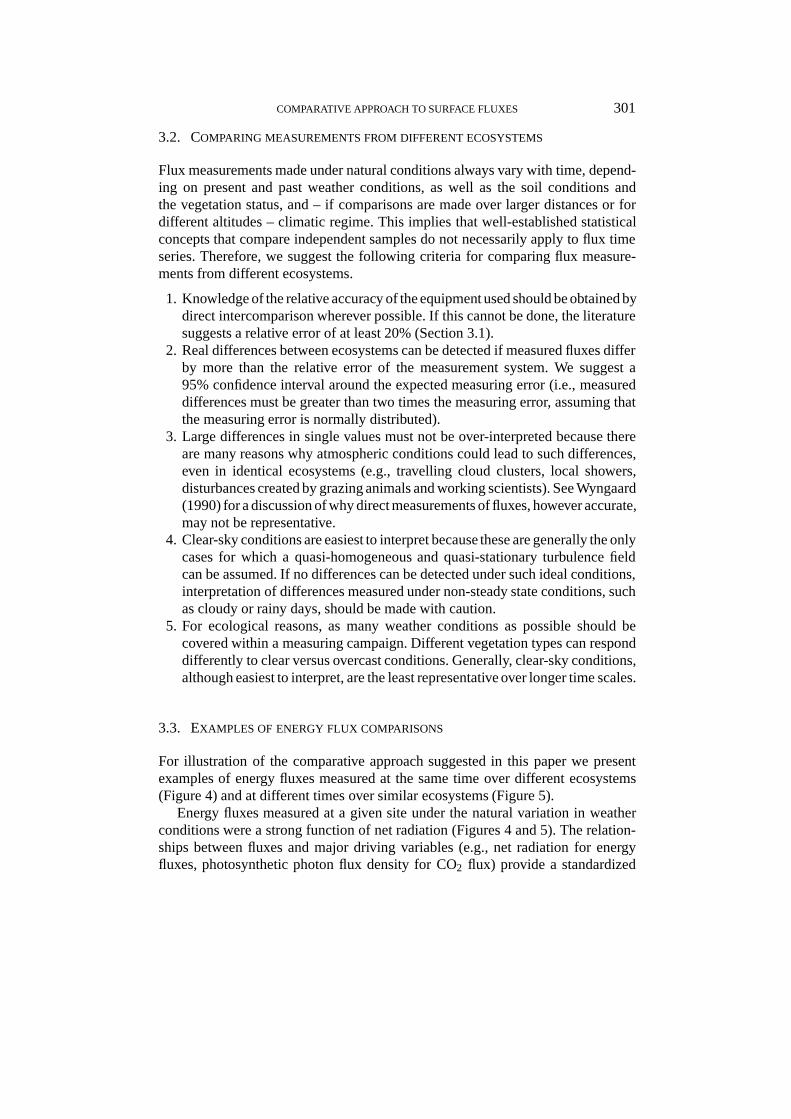
3.2. COMPARING MEASUREMENTS FROM DIFFERENT ECOSYSTEMS

Flux measurements made under natural conditions always vary with time, depend-ing on present and past weather conditions, as well as the soil conditions andthe vegetation status, and – if comparisons are made over larger distances or fordifferent altitudes – climatic regime. This implies that well-established statisticalconcepts that compare independent samples do not necessarily apply to flux timeseries. Therefore, we suggest the following criteria for comparing flux measure-ments from different ecosystems.

1. Knowledge of the relative accuracy of the equipment used should be obtained bydirect intercomparison wherever possible. If this cannot be done, the literaturesuggests a relative error of at least 20% (Section 3.1).

2. Real differences between ecosystems can be detected if measured fluxes differby more than the relative error of the measurement system. We suggest a95% confidence interval around the expected measuring error (i.e., measureddifferences must be greater than two times the measuring error, assuming thatthe measuring error is normally distributed).

3. Large differences in single values must not be over-interpreted because thereare many reasons why atmospheric conditions could lead to such differences,even in identical ecosystems (e.g., travelling cloud clusters, local showers,disturbances created by grazing animals and working scientists). See Wyngaard(1990) for a discussion of why direct measurements of fluxes, however accurate,may not be representative.

4. Clear-sky conditions are easiest to interpret because these are generally the onlycases for which a quasi-homogeneous and quasi-stationary turbulence fieldcan be assumed. If no differences can be detected under such ideal conditions,interpretation of differences measured under non-steady state conditions, suchas cloudy or rainy days, should be made with caution.

5. For ecological reasons, as many weather conditions as possible should becovered within a measuring campaign. Different vegetation types can responddifferently to clear versus overcast conditions. Generally, clear-sky conditions,although easiest to interpret, are the least representative over longer time scales.

3.3. EXAMPLES OF ENERGY FLUX COMPARISONS

For illustration of the comparative approach suggested in this paper we presentexamples of energy fluxes measured at the same time over different ecosystems(Figure 4) and at different times over similar ecosystems (Figure 5).

Energy fluxes measured at a given site under the natural variation in weatherconditions were a strong function of net radiation (Figures 4 and 5). The relation-ships between fluxes and major driving variables (e.g., net radiation for energyfluxes, photosynthetic photon flux density for CO2 flux) provide a standardized


−100 0 100 200 300 400 500−100

−50

0

50

100

150

200

250W

m−

2

0.25 Rn

0.39 Rn

−100 0 100 200 300 400 500−100

−50

0

50

100

150

200

250

W m

−2

0.39 Rn

0.34 Rn

−100 0 100 200 300 400 500Net Radiation, W m

−2

−100

−50

0

50

100

150

200

250

W m

−2

0.27 Rn

0.11 Rn

sensible heat flux

latent heat flux

ground heat flux

Figure 4. Relationships of sensible heat, latent heat and ground heat fluxes to net radiation for twodifferent ecosystems—riparian shrub (open circles, dotted regression lines) and watertrack (crosses,solid regression lines) measured at the same time (10–18 July 1995). Values in legends are theregression coefficients. Data points are 30-minute averages.


−100 0 100 200 300 400 500−100

−50

0

50

100

150

200

250W

m−

2

0.37 Rn

0.42 Rn

−100 0 100 200 300 400 500−100

−50

0

50

100

150

200

250

W m

−2

0.28 Rn

0.26 Rn

−100 0 100 200 300 400 500Net Radiation, W m

−2

−100

−50

0

50

100

150

200

250

W m

−2

0.16 Rn

0.13 Rn

sensible heat flux

latent heat flux

ground heat flux

Figure 5. As in Figure 4, but for two sites of the same ecosystem type (moist acidic tussock tundra)measured at different times and at different locations—Sagwon Hills, a relatively warm site, 21–29 June 1995 (open circles, dashed regression lines) and Toolik Lake, a cold, high-elevation site,approximately 80 km to the south, 19 July to 1 August 1995 (crosses, solid regression lines).


way to compare fluxes among sites measured at different times under differentconditions (Figure 5). The relationship between net radiation and energy fluxes hasbeen used previously to extrapolate fluxes diurnally at a single site (e.g., de Bruinand Holtslag, 1982; Jackson et al., 1983; Whiteman et al., 1989; Brutsaert andSugita, 1992).

The two sites compared in Figure 4, a riparian shrub ecosystem (predominantlywillow shrubs on sandy fluvial soils) and a watertrack ecosystem (willow shrubsalong wet watertracks, dwarf-birch shrubs on drier rims), are different in soilmoisture availability and species composition. Based on criterion 2 given above,we find differences in sensible heat and ground heat fluxes, while latent heat fluxesdo not differ significantly. The riparian site had greater ground heat flux at high netradiation and greater heat loss at low radiation, compared to the watertrack, becausethe moist sandy surface soil in the frequently flooded riparian site conducted heatmore readily than did the highly insulative moss surface of the watertrack. Theresulting difference in temperature of the soil/moss surface contributed to thegreater sensible heat flux of the watertrack compared to the riparian shrub. Coldair drainage also promoted negative ground heat flux at night in the valley-bottomriparian site.

In Figure 5 we compare moist acidic tussock tundra, an ecosystem type verycommon in the low arctic, between two sites located 80 km from each other, withslightly different climates due to latitudinal and altitudinal differences. We found nosignificant differences in sensible or latent heat fluxes as a function of net radiation,despite the different climates and different times in the growing season. However,the fraction of net radiation dissipated to ground heat flux was 20% lower at ToolikLake than at Sagwon Hills. We expect that this difference is mainly due to smallerdifferences between air and soil temperatures at Toolik Lake, a higher elevationsite in the foothills of the Brooks Range.

The energy fluxes that we measured do not always add up to 100% because wedid not force our regressions through the origin. Non-zero intercepts are physicallyreasonable in the Arctic, where high surface moisture, cold soils, and 24-h tran-spiration promote fluxes even at low radiation. Site differences in fluxes at zeronet radiation (non-zero intercept) could be ecologically important and contributeto seasonal differences among sites in ground heat flux and soil thermal regime.

The major disadvantage of mobile towers is that they cannot provide an integrat-ed annual estimate of any flux. However, if a reference tower is run continuously,and comparisons are made between mobile towers and the reference tower formajor seasons, estimates can be made at many sites with a relatively small numberof flux towers. Conversely, an approach using mobile towers to simultaneouslymeasure different fluxes from ecosystem types in close proximity provides the firstmethod for rigorous comparison of fluxes among ecosystems.

Estimates of annual carbon flux often differ substantially among years for agiven site (Wofsy et al., 1993; Goulden et al., 1996), making it difficult to compare


carbon fluxes among ecosystems that are measured in different years, althoughpartitioning of energy fluxes may not show as much of a difference.

We suggest that use of mobile towers allows a rapid comparison of ecosystemswith respect to surface fluxes. This will be particularly useful for comparison ofwater and energy fluxes, where it is usually more important to know flux withrespect to ecological and environmental drivers than to know integrated annualfluxes.

4. Conclusions

Mobile towers are an economical approach to determining ecosystem-scale con-trols on surface fluxes – a step that is essential for landscape-scale estimates offluxes needed to validate regional and global models. Furthermore, mobile towermeasurements complement permanent-tower observations, because it is not possi-ble for relatively few and widely separated long-term flux monitoring stations toadequately characterize an entire region, and because the locations of long-termstations usually are constrained by logistical limitations (road access, power supply,proximity to year-round settlements where technicians are based). Mobile towermeasurements are important to put flux data from long-term monitoring stationsinto the context of the actual landscape-scale variability of a region.

Acknowledgements

This project is part of the Arctic System Science Flux Study funded by the U.S.National Science Foundation (OPP-9318532). We thank Dr. Hans Peter Schmid,University of Indiana, Bloomington, U.S.A., for use of the source code of hisFlux Source Area Model, version 2.10; George Vourlitis and Walter C. Oechel,San Diego State University, U.S.A., for access to their unpublished data from twopermanent reference towers; and Gaius Shaver and James Laundre, Toolik LakeLong-Term Ecological Research (LTER) site, for meteorological station recordsfrom 1995 and 1996.

References

Arya, S. P. S.: 1988, Introduction to Micrometeorology, Academic Press, San Diego, 307 pp.Auble, D. L. and Meyers, T. P.: 1992, ‘An Open Path, Fast Response Infrared Absorption Gas Analyzer

for H2O and CO2’, Boundary-Layer Meteorol. 59, 243–256.Auerbach, N. A. and Walker, D. A.: 1995, ‘Preliminary Vegetation Map, Kuparuk River Basin,

Alaska: A Landsat-Derived Classification’, Unpublished.Brutsaert, W. and Sugita, M.: 1992, ‘Application of Self-Preservation in the Diurnal Evolution of the

Surface Energy Budget to Determine Daily Evaporation’, J. Geophys. Res. 97, 18377–18382.


de Bruin, H. A. R. and Holtslag, A. A. M.: 1982, ‘Simple Parametrization of the Surface Fluxes ofSensible and Latent Heat During Daytime Compared with the Penman-Monteith Concept’, J.Appl. Meteorol. 21, 1610–1621.

Dugas, W. A.: 1992, ‘Bowen Ratio and Eddy Correlation Measurements for Bare Soil, Sorghum, andRangeland’, Wetter und Leben 44, 3–16.

Eugster, W. and Senn, W.: 1995, ‘A Cospectral Correction Model for Measurement of Turbulent NO2

Flux’, Boundary-Layer Meteorol. 74, 321–340.Fitzjarrald, D. R. and Moore, K. E.: 1992, ‘Turbulent Transports Over Tundra’, J. Geophys. Res. 97,

16717–16729.Foken, T. and Wichura, B.: 1996, ‘Tools for Quality Assessment of Surface-Based Flux Measure-

ments’, Agric. For. Meteorol. 78, 83–105.Garratt, J. R.: 1994, The Atmospheric Boundary Layer, Cambridge University Press, Cambridge,

316 pp.Goulden, M. L., Munger, J. W., Fan, S.-M., Daube, B. C., and Wofsy, S. C.: 1996, ‘Exchange of

Carbon Dioxide by a Deciduous Forest: Response to Interannual Climate Variability’, Science271, 1576–1578.

Harazono, Y., Yoshimoto, M., Miyata, A., Uchida, Y., Vourlitis, G. L., and Oechel, W. C.: 1995,Micrometeorological Data and Their Characteristics over the Arctic Tundra at Barrow, Alas-ka During the Summer of 1993, No. 16 in Misc. Publications, National Institute of Agro-Environmental Sciences, Kannondai, Tsukuba, Japan, 215 pp.

Harazono, Y., Yoshimoto, M., Vourlitis, G. L., Zulueta, R. C., and Oechel, W. C.: 1996, ‘Heat, Waterand Greenhouse Gas Fluxes Over the Arctic Tundra Ecosystems at Northslope in Alaska’, inProc. IGBP/BAHC-LUCC 4–7 November 1996, Kyoto, Japan, pp. 170–173.

Haugen, D. A., Kaimal, J. C., and Bradley, E. F.: 1971, ‘An Experimental Study of Reynolds Stressand Heat Flux in the Atmospheric Surface Layer’, Quart. J. Roy. Meteorol. Soc. 97, 168–180.

Jackson, R. D., Hatfield, J. L., Reginato, R. J., Idso, S. B., and Pinter, P. J., Jr.: 1983, ‘Estimationof Daily Evapotranspiration From one Time of Day Measurements’, Agric. Water Manage. 7,351–362.

Jones, H. G.: 1992, Plants and Microclimate, Cambridge University Press, Cambridge, 2nd edn., 428pp.

Laubach, J.: 1996, Charakterisierung des turbulenten Austausches von Warme, Wasserdampf undKohlendioxid uber niedriger Vegetation anhand von Eddy-Korrelations-Messungen, 3 of Wis-senschaftliche Mitteilungen, Inst. fur Meteorologie und Inst. fur Tropospharenforschung, Univ.Leipzig, 139 pp.

McMillen, R. T.: 1988, ‘An Eddy Correlation Technique With Extended Applicability to Non-SimpleTerrain’, Boundary-Layer Meteorol. 43, 231–245.

Nie, D., Kanemasu, E. T., Fritschen, L. J., Weaver, H. L., Smith, E. A., Verma, S. B., Field, R. T.,Kustas, W. P., and Stewart, J. B.: 1992, ‘An Intercomparison of Surface Energy Flux MeasurementSystems Used During FIFE 1987’, J. Geophys. Res. 97, 18715–18724.

Oechel, W. C., Hastings, S. J., Vourlitis, G., Jenkins, M., Riechers, G., and Grulke, N.: 1993, ‘RecentChange of Arctic Tundra Ecosystems From a Net Carbon Dioxide Sink to a Source’, Nature 361,520–523.

Panofsky, H. A. and Dutton, J. A.: 1984, Atmospheric Turbulence, John Wiley & Sons, New York,397 pp.

Rachidi, F., Kirkham, M. B., Kanemasu, E. T., and Stone, L. R.: 1993, ‘Energy Balance Comparisonof Sorghum and Sunflower’, Theoret. Appl. Climatol. 48, 29–39.

Schmid, H. P. and Oke, T. R.: 1990, ‘A Model to Estimate the Source Area Contributing to TurbulentExchange in the Surface Layer Over Patchy Terrain’, Quart. J. Roy. Meteorol. Soc. 116, 965–988.

Stull, R. B.: 1988, An Introduction to Boundary Layer Meteorology, Kluwer Academic Publishers,Dordrecht, 666 pp.

Whiteman, C. D., Allwine, K. J., Fritschen, L. J., Orgill, M. M., and Simpson, J. R.: 1989, ‘DeepValley Radiation and Surface Energy Budget Microclimates. Part II: Energy Budget’, J. Appl.Meteorol. 28, 427–437.


Wofsy, S. C., Goulden, M. L., Munger, J. W., Fan, S.-M., Bakwin, P. S., Daube, B. C., Bassow,S. L., and Bazzaz, F. A.: 1993, ‘Net Exchange of CO2 in a Mid-Latitude Forest’, Science 260,1314–1317.

Wyngaard, J. C.: 1990, ‘Scalar Fluxes in the Planetary Boundary Layer – Theory, Modeling, andMeasurement’, Boundary-Layer Meteorol. 50, 49–75.

Yoshimoto, M., Harazono, Y., Miyata, A., and Oechel, W. C.: 1996a, ‘Micrometeorology and HeatBudget over the Arctic Tundra at Barrow, Alaska in the Summer of 1993’, J. Agric. Meteorol. 52,11–20.

Yoshimoto, M., Harazono, Y., and Oechel, W. C.: 1997, ‘Effects of Micrometeorology on the CO2

Budget in Mid-summer over the Arctic Tundra at Prudhoe Bay, Alaska’, J. Agric. Meteorol. 53,1–10.

Yoshimoto, M., Harazono, Y., Vourlitis, G. L., and Oechel, W. C.: 1996b, ‘The Heat and WaterBudgets in the Active Layer of the Arctic Tundra at Barrow, Alaska’, J. Agric. Meteorol. 52,293–300.

Documents

WERNER EUGSTER, JOSEPH P. MCFADDEN and F ...homepage.agrl.ethz.ch/~eugsterw/publications/pdf/Eugster...WERNER EUGSTER, JOSEPH P. MCFADDEN and F. STUART CHAPIN, III Department of Integrative