RESEARCH ARTICLE - APPLIED GEOPHYSICS

Well-log based rock physics template of the Vienna Basinand the underlying Calcereous Alps

Nebojsa Tucovic1 • Nina Gegenhuber1

Received: 30 December 2016 / Accepted: 30 March 2017 / Published online: 13 April 2017

� The Author(s) 2017. This article is an open access publication

Abstract In this study, the ratio of compressional and

shear wave velocity versus acoustic impedance as rock

physics template for northern part of the Vienna Basin has

been derived for siliciclastic rocks based on formation

evaluation of well-log data. The results have been verified

through wells in different areas drilled in various depths.

Additionally, depositional sequences like prograding deltas

and braided rivers have been plotted onto the rock physics

template to illustrate the effect of changing shale volume.

Carbonates below the basin have been included into the

study and results from previous projects, based on labora-

tory data and petrophysical models on certain lithologies in

the Vienna Basin, have been used to compare the outcome.

The result is a rock physics template which includes

important properties such as porosity, true vertical depth

and fluid type from log data and which is considered use-

able throughout different areas and various lithologies of

the Vienna Basin.

Keywords Rock physics template � Formation evaluation �Vienna Basin � Depositional sequences

Introduction

Seismic measurements are the most frequently used

methods in exploration activities in the oil and gas indus-

try. More advanced and complex tools to get more quali-

tative as well as quantitative information out of a seismic

cube have been developed through the last decades. Øde-

gaard and Avseth (2009) published the so-called rock

physics template (RPT). Their idea was to create basin and

lithology-dependent templates mainly with elastic proper-

ties of rocks (most commonly the ratio of compressional

and shear wave velocity (vp/vs) and acoustic impedance

(AI)) of rocks. These templates, which are able to indicate

fluid and lithology trends, can then be used for interpre-

tation of seismic data from the corresponding basin or

lithology. In further consequence rock physics templates

have been widely used in the exploration activities within

the industry. Numerous studies have been conducted. Most

of the studies used elastic properties in siliciclastic rocks to

construct the templates with petrophysical models (Avseth

et al. 2009; Chi and Han 2009; Gupta et al. 2012).

Rock physics templates for carbonate reservoirs have

been created too. Ba et al. (2013) created multiscale rock

physics templates for carbonates and validated them with

laboratory, well and seismic data. Gegenhuber and Pupos

(2015) determined elastic properties with Hashin and

Shtrikman (1962) bounds and derived vp/vs–acoustic

impedance-based rock physics templates from laboratory

data for three different carbonate types from Austria under

dry and wet conditions, applied additionally on log and

seismic data (Pupos 2015).

Avseth and Veggeland (2015) introduced additional

rock stiffness/rock impedance (PEIL) and fluid softness/

fluid impedance (CPEI) attributes which honour funda-

mental rock physics from vp/vs–AI rock physics templates.

The combined use of these two attributes can help differ-

entiate between fluid and lithology anomalies in the rock

physics template. Additionally, Avseth and Carcione

(2015) used rock physics templates to get an understanding

of complex kerogen-rich Jurassic source rocks from the

Norwegian Shelf. vp/vs–acoustic impedance behaviour

& Nina Gegenhuber

nina.gegenhuber@unileoben.ac.at

1 Chair of Applied Geophysics, Montanuniversitaet, Leoben,

Austria

123

Acta Geophys. (2017) 65:441–451

DOI 10.1007/s11600-017-0037-6

throughout the different processes in the compaction and

hydrocarbon generation of source rocks helps to determine

the maturity of the rock and generation of hydrogen.

Hermana et al. (2016) derived rock physics templates

from attenuation parameters (SQp and SQs) and applied it

to a real dataset from Malay Basin. They concluded that

their attenuation-based rock physics templates derive better

lithology and fluid separation results than conventional vp/

vs–acoustic impedance rock physics templates on the

considered dataset. Tucovic et al. (2016) created resistiv-

ity–acoustic impedance rock physics templates based on

deep reading logging while drilling data as a foundation for

further work of real-time template-based logging while

drilling interpretation for enhanced geosteering operations.

Although all these rock physics templates are able to

distinguish between gas and water and different lithologies,

they are still not suitable for determining oil saturation

within seismic data and are mainly usable just for one

lithology with certain properties throughout the basin.

As pointed out, RPTs are a valuable tool in seismic

exploration industry. The goal of this paper is to create a

rock physics template which is applicable in the whole

pull-apart basin in Lower Austria and the underlying Cal-

careous Alps with well-log based formation evaluation.

Parts are evaluated with derived RPTs out of laboratory

data. Depth-related trends are considered as well as dif-

ferent lithologies with their evaluated properties from for-

mation evaluation of the logs. Depositional sequences like

prograding deltas or braided rivers are visualized on the

created template to validate it.

Geology of the Vienna Basin

Vienna Basin is a 200-km-long and 60-km-wide rhombic

pull-apart basin located in the northeast part of Austria. It is

a mature basin operated by OMV since the 1930s. The

basement of the Vienna Basin is the Bohemian Massif

overlain by the autochthonous sedimentary cover which is

Jurassic to Cretaceous age (Ladwein 1988). This sedi-

mentary cover is followed by the Flysch Zone (Lower

Cretaceous–Eocene) and finally the Northern Calcareous

Alps (Permian–Cretaceous), which have been overthrusted

during the northwest-directed transportation in lower Cre-

taceous–Oligocene age with piggy back basins on their

back. After the thrusting in the middle Miocene (Bade-

nian), north south compression with associated compen-

sation movement of the nappes to northeast occurred. This

resulted in separation of the Northern Calcareous Alps and

Carpathians associated to extension and pull-apart effects

(Wessely 2006). During this time, main subsidence and

sedimentation of clastic sediments as a result of trans-

gressive/regressive cycles due to sea level changes took

place (Kreutzer 1992). Thus, the sediments of the Vienna

Basin are of Neogene age and reach 5–6 km at some

locations (Ladwein 1988).

Early stages of basin development in Ottnangian and

Karpatian are dominated by lacustrine to fluvial environ-

ment while in Badenian (Middle Miocene) transgressive/

regressive cycles with prograding deltas in marine envi-

ronment are dominating (Sauer et al. 1992). Here the most

reservoirs in the Vienna Basin are saturated and the sand

horizons are numbered. An example is 16th TH (Tortonian

horizon) which consists of many on-lapping layers, which

are composed of prograding delta front sequences and

separated by flooding events. By the side, already more

than 400 wells have been drilled into this 16th TH, also

called the Matzen sand and the associated Matzen giant

field which has been discovered in 1949 and is one of the

largest multi-pool oil and gas field onshore Europe

(Kienberger and Fuchs 2006). In the following Sarmatian,

marine environment evolved to brackish water conditions

and lead to lacustrine and fluvial deposits in the Pannonian

(Sauer et al. 1992). Up to 20 sand horizons have been

deposited and numbered here throughout the basin. After

the Sarmatian, during the Pannonian sedimentation con-

tinued in lacustrine environment with deposition of fluvi-

atile clastic sediments.

Besides the huge number of reservoirs within the Neo-

gene part of the succession, commercial pay zones have

been found within the Triassic dolomites underneath the

Basin in the allochthonous nappes (Ladwein 1988). This

dolomite called the ‘‘main dolomite’’ is formed in shallow

lagoon areas and shallow water zones with very low

porosity (Gegenhuber and Pupos 2015). Main source rocks

in the basin are the Upper Jurassic (Malmian) marls in the

autochthonous part of the section (Hamilton et al. 1999),

which are generated below the basin in depths of 3–6 km

(Ladwein 1988). Sachsenhofer (2001) identified a

geothermal gradient of the basin of 30 �C/km.

Data and methodology

Data

Data used are wireline log data from the northern part of

Vienna Basin. Most of data are available from Field A,

which is situated on a structural high. Thus, wells which

have been used for creation of rock physics templates from

this field have reached true vertical depths (TVD) of about

2.3 km. Other fields are located in deeper areas of the

basin, mainly on structural low, but still in the northern

part. One well per field have been used in Field B (true

vertical depth of about 4.1 km), Field C and D (true ver-

tical depths of about 3 km). A simple sketch to illustrate

442 Acta Geophys. (2017) 65:441–451

123

the wells from different fields is shown in Fig. 1. The three

wells in other areas of the basin (Field B, C and D) have

been mainly used to evaluate the rock physics templates

created with detail-evaluated wells from shallower areas

from Field A because they encountered the same and

similar siliciclastic rocks in much greater depths.

Table 1 shows the encountered formations and their

horizons within the wells with the corresponding ages. Ages

in the second column are from Central Paratethys nomen-

clature. Third column indicates the availability of hydro-

carbons within the corresponding formations throughout the

basin. In the last column the four fields are indicated which

have the necessary data (shear velocity was the limiting

factor) to create a rock physics template. As visible, ‘‘the

main dolomite’’ from the Calcareous Alps beneath the basin

has been drilled in the deep well in Field D too.

Methodology

Formation evaluation of Field A wells

To create a rock physics template from log data alone, it is

necessary to complete a full formation evaluation of the

investigated wells. This has been done with well mea-

surement data from Field A. Formation tops, lithology

discrimination, reservoir identification and fluid type and

saturation have been fully determined within the Field A.

The next step was to pick out shale and sand intervals to

create model rock physics template shale and sand lines.

These have been picked after the criteria defined in

Table 2. Additionally, sand has been differentiated after

the various fluid contents (gas, oil, water).

In Fig. 2, an example of log representation of a hydro-

carbon reservoir with surrounding shale deposited in early

Miocene is shown. The first track shows picked lithology

and fluid intervals for the rock physics template. This

reservoir sand has gas- and oil-bearing zones and is over-

and underlain by shale layers.

With data from shale and sand (water–oil–gas) horizons

from Field A, a scatter plot with four variables (resistivity,

acoustic impedance, density and vp/vs) and two-dimen-

sional combinations are determined. It was used to see

where the best fluid and lithology separation can be

achieved. As used by numerous studies in the past, vp/vs–

acoustic impedance crossplot has shown best results for

fluid and lithology discrimination.

Choosing the right two-dimensional crossplot

for differentiation

Figure 3 shows scatter plot with resistivity, acoustic

impedance, vp/vs ratio and density of the picked fluid-dis-

criminated sand horizons and shale layers. It is clearly

visible that green (oil reservoirs) and red (gas reservoirs)

points are plotting always in areas of higher formation

resistivity. Blue data points, which represent water-bearing

sand horizons are slightly separated from shales coloured

in brown. Note the significant oil/gas separation in density-

included crossplots. Resistivity-included crossplots sepa-

rate well between hydrocarbon and water. Thus, density–

resistivity and acoustic impedance–resistivity crossplots

(indicated with a red dashed circle) are very good fluid

discriminators. On the other side, lithology (shale–sand) is

not sufficiently separated in these crossplots. From first

look onto the crossplots best results regarding lithology

discrimination are reached at acoustic impedance–vp/vs and

density–vp/vs crossplots (marked with the blue dashed cir-

cle). Thus, for this study standard acoustic impedance–vp/vscrossplot is chosen.

Modelling the rock physics template with well data

from Field A

In the next step, elastic data from the picked horizons from

formation evaluation in wells from Field A is plotted onto a

vp/vs–AI crossplot. Figure 4 shows lithology-discriminated

data points from these wells including shale and sand.

Shale and sand lines have been fitted to the data. Shale line

is modelled above the shale data points (brown) because

below this line the shale is getting mixed with silt and sand.

Sand line on the other side has been modelled below the

water-saturated sand points because above the sand is

getting mixed with clay.

Fig. 1 Simple sketch illustrating the shallow Field A wells on

structural highs and Field B–D wells on structural lows

Acta Geophys. (2017) 65:441–451 443

123

Thus, between these two lines on the crossplot the

lithology is a mixture between sand and shale. The scat-

tering of the sand–shale data points results from the fact

that sand and shale lithologies are hardly clean in the field

data (100% sand/clay content). As shown in Table 2, shale

horizons have been picked, if shale volume is bigger than

60%. Red line represents 100% gas saturation in sands and

is modelled below the picked gas-bearing reservoir inter-

vals because they are not 100% gas-saturated. Note the

green points slightly below the 100% water saturation sand

line which represent picked oil-bearing reservoirs, most of

them in Badenian ages.

After the curve fitting and determination of corre-

sponding shale, sand (water and gas) lines for the Field A

lithologies in the Vienna Basin, additional information of

well-log interpretation have been used to model other rel-

evant properties onto the template. Unlike Fig. 4 which

shows just picked sand and shale lithologies, the four

crossplots in Figs. 5 and 6 show all data points from wells

within the Field A with modelled shale and gas/water sand

lines.

In each crossplot different colour scales have been used

which have been delivered from formation evaluation of

the Field A wells. Left crossplot in Fig. 5 has total porosity

as colour scale with determined porosity isolines. The

crossplot on the right in Fig. 5 shows the same data points

from wells from Field A with true vertical depth as colour

scale. Here it is more difficult to distinguish between dif-

ferent TVD trends resulting in higher uncertainty of the

true vertical depth trendlines. Isolines are directly drawn in

the plot, using the colour code from the porosity and depth.

In the two crossplots in Fig. 6, same data from Field A

as in Fig. 5 is plotted with shale volume (left) and water

saturation (right) as colour scale. As excepted the shale

volume and the water saturation values show the predicted

plotting behaviour. Water-saturated formations (shales and

water-saturated sands) plot above the blue water line and

below the shale line while hydrocarbon-saturated reservoirs

plot below. Low shale volume (where clean sand can be

assumed) fits the sand line (and the gas-bearing direction)

quite well. Exception is some shallow low shale areas

which are indicated in the crossplot. Here it is assumed that

the compressional velocity measurements are not valid

anymore because of the low compaction and high porosity

of the formation.

Validating the rock physics template with deeper wells

from Field B, C and D

In the next step, the determined shale and sand lines fromwells

in Field A have been validated with wells, which drilled the

same and similar siliciclastic formations in bigger depths.

Each crossplot in Fig. 7 shows data from one well drilled in

different fields and in different area of the northern part of the

Vienna Basin. As described in the data chapter before, these

Table 1 Encountered and evaluated formations within the study which have been used for creation of rock physics templates

Age Age (Tethys) Reservoir Subage/formation Horizons Elastic data available

Miocene Pontian – Pontian – –

Pannonian G Middle Pannonian Middle Pannonian horizon Field A

G Lower Pannonian Lower Pannonian horizon Field A

Sarmatian O & G Upper Sarmatian Sarmatian horizon Field A

O & G Lower Sarmatian Sarmatian horizon Field A

Badenian O Buliminen Rotalien zone – Field A, B (deep), C (deep)

O & G Sandschaler zone Tortonian horizons Field A, B (deep), C (deep)

O & G Upper Lageniden Lower Tortonian horizon Field A, B (deep), C (deep)

– Aderklaa Conglomerate – Field A, B (deep), C (deep)

Karpatian – Aderklaa formation – Field C (deep), D (deep)

G Gaenserndorf formation – Field C (deep), D (deep)

Ottnangian O Bockflies formation – Field D (deep)

Eggenburgian – Missing in study area – –

Trias. N. Calc. Alps O & G Main dolomite – Field D (deep)

All used formations in this study except the Triassic ‘‘main dolomite’’ have been deposited during the Miocene. Most reservoirs have been

deposited in mid-Miocene during Badenian time

G gas, O oil

Table 2 Lithology and fluid discrimination criteria within the logs

Shale [60% Vsh

Sand_water-bearing \20% Vsh & Sw[80%

Sand_gas-bearing \20%Vsh & Sw\50% and logs indicate gas

Sand_oil-bearing \20%Vsh & Sw\50% and logs indicate oil

444 Acta Geophys. (2017) 65:441–451

123

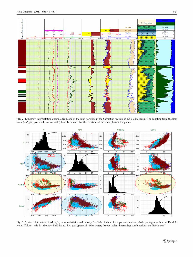
Fig. 2 Lithology interpretation example from one of the sand horizons in the Sarmatian section of the Vienna Basin. The zonation from the first

track (red gas; green oil; brown shale) have been used for the creation of the rock physics templates

Fig. 3 Scatter plot matrix of AI, vp/vs ratio, resistivity and density for Field A data of the picked sand and shale packages within the Field A

wells. Colour scale is lithology–fluid based. Red gas; green oil; blue water; brown shales. Interesting combinations are highlighted

Acta Geophys. (2017) 65:441–451 445

123

wells are mainly located in structural lows with the same

formations encountered approximately 1.5 km deeper than

the wells from Field A.

Thus, note the different x-axes from previous vp/vs–AI

crossplots (starting atAI = 7000 g m/cm3 s).Asvisible in the

crossplot, the encountered lithologies, consisting mainly of

shales and sands from Badenian, Karpatian and Ottnangian

ages of theFieldB,C andDwells are fitting verywell between

the sand and shale line derived from Field A. Ottnangian (first

crossplot, brown data points),which consistsmainly of shales,

Fig. 4 vp/vs versus AI rock physics template with the shale (brown) and sand (red gas; green oil; blue water) zonation from the Field A wells.

Modelled shale, water sand and gas sand lines with their equations are displayed too

Fig. 5 vp/vs–AI crossplots from all wells (Field A) with modelled shale, water–sand and gas–sand lines. On the left total porosity is used as

colour scale and on the right TVD is used as colour scale. Some porosity and TVD isolines are indicated on each crossplot

446 Acta Geophys. (2017) 65:441–451

123

plots slightly below the modelled shale line. ‘‘The main

dolomite’’ below the basin, which has been drilled by awell in

FieldDplots in area slightly below vp/vs ratio of 2 and acoustic

impedance of above 15000 g m/cm3 s.

Results and interpretation

In the following section, lithology and fluid effects and the

influence of different depositional sequences within the

Vienna Basin on the plotting behaviour and the derived shale

and sand lines within the Neogene sequence of the Vienna

Basin, as well as ‘‘the main dolomite’’ beneath will be

interpreted and discussed. Additionally, data will be com-

pared to already existing rock physics templates derived by

laboratory measurements and petrophysical models.

The created rock physics template follows the trendswhich

has already been shown in numerous studies and discussed

and summarized, e.g. byAvseth et al. (2005) or Schon (2015):

– Gas saturation decreases vp/vs ratios and acoustic

impedance.

Fig. 6 vp/vs–AI crossplots from wells (Field A) with modelled shale, water–sand and gas–sand lines. On the left calculated shale volume is used

as colour scale and on the right calculated water saturation has been used as colour scale

Fig. 7 All available data from the remaining wells (vs limiting

factor) plotted on a vp/vs–AI crossplot with shale and sand (water and

gas) lines derived from Field A wells. Note that the starting point of

the x-axes is different from the previous crossplots (7000 g m/cm3 s)

due to the deeper depth of investigated formations

Acta Geophys. (2017) 65:441–451 447

123

– Shale content increases vp/vs ratios and decreases

acoustic impedance.

– Compaction decreases vp/vs ratios and increases acous-

tic impedance.

– Porosity slightly increases vp/vs ratios and decreases

acoustic impedance.

– Oil–water contrasts are hardly recognized with elastic

measurements.

The last point, which states out that oil–water contrasts

are hardly recognized with elastic measurements due to

similar oil and water densities, is true, but as visible in

Fig. 3 the green points (oil-bearing reservoirs) have sig-

nificantly different plotting areas compared to the blue

water-saturated sands. Thus, in Vienna Basin it could be

possible to define oil-bearing sand area and to try to read

them out of seismic. Gas-bearing horizons are clearly

separated from water and oil-bearing sands due to the

different elastic properties of the fluids.

The porosity trend shown in Fig. 4 indicates a good

correlation with the elastic parameters and the above

statement from previous studies is given. However, when

looking at different lines (water/gas sand and shale) at

same acoustic impedance on the x-axis, porosity of gas-

bearing sand is the lowest followed by shale and last but

not least water-bearing sand. This is the same trend shown

in previous studies (e.g. Avseth et al. 2005). In true vertical

depth colour-scaled crossplot in the same figure, the true

vertical depth gradients show similar behaviour although

there are some uncertainties in these isolines as stated out

before and visible on the crossplot. Reasons for the

uncertainty of true vertical depth trendlines could be the

faulting of the basin and the related different compaction

rate depending on the, e.g. hanging or footwall side of the

fault and the timing of the fault. Another reason for the

uncertainty of the true vertical depth lines could be the

deviation of the drilled wells and the tool during the

measurements. Anisotropic shale formations will result in

higher velocity measurements when measured under

deviated conditions than when the well is fully vertical at

the same true vertical depth and compaction behaviour.

Nevertheless, the modelled true vertical depth trend lines

still are showing predicted behaviour and can be used for

further investigations.

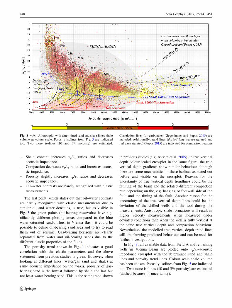
In Fig. 8, all available data from Field A and remaining

wells in Vienna Basin are plotted onto vp/vs–acoustic

impedance crossplot with the determined sand and shale

lines and porosity trend lines. Colour scale shale volume

has been chosen. Porosity isolines from Fig. 5 are indicated

too. Two more isolines (10 and 5% porosity) are estimated

(dashed because of uncertainty).

Fig. 8 vp/vs–AI crossplot with determined sand and shale lines; shale

volume as colour scale. Porosity isolines from Fig. 5 are indicated

too. Two more isolines (10 and 5% porosity) are estimated.

Correlation lines for carbonates (Gegenhuber and Pupos 2015) are

included. Additionally, sand lines (dashed blue water-saturated and

red gas-saturated) (Pupos 2015) are indicated for comparison reasons

448 Acta Geophys. (2017) 65:441–451

123

Hashin–Shtrikman bounds from previous work from

Gegenhuber and Pupos (2015) on dry (black) carbonate

samples (including ‘‘main dolomite’’) are plotted on the

right side of the template. Within that study saturated

bounds have been derived too, but due to the fact that

dolomite here is dry only dry bounds are shown in the

crossplot.

Additionally, for comparison reasons data derived from

laboratory measurements on plugs (siliciclastic lithology

water-bearing and gas-bearing sand) are indicated in

dashed thin blue and red lines with the derived porosity.

These plugs are from Badenian age sand reservoirs from

Vienna Basin and modelled with petrophysical models

(Cement models (Dvorkin and Nur 1996 and Avseth et al.

2000), Hashin–Shtrikman bounds (1962), and Gassmann

fluid substitution (Gassmann 1951). The lines are results of

an unpublished master thesis related to rock physics tem-

plates in Vienna Basin (Pupos 2015).

As visible, there are two main areas of the crossplot.

Data points from the Neogene (Miocene) siliciclastic

lithology of the Vienna Basin itself are on the left side with

lower acoustic impedance values and data points from the

northern Calcareous Alps, i.e. the dense and low-porosity

‘‘main dolomite’’ are on the right side in areas of higher

acoustic impedance values. Therefore, a kind of petro-

graphic code (=influence of mineralogy/lithology) is visi-

ble. When considering the shale volume colour scale of all

available data, the shale and sand lines fit very well to the

data. Below the blue 100% water saturation line most of

the data are taken from hydrocarbon-bearing reservoirs,

above the sand is less clean.

Equations 1–3 below represent the sand and shale

regression lines which have been derived through the curve

fitting on the well data as described in the methodology

chapter.

Shale:Vp

Vs

¼ 90:4 � AI�0:416 ð1Þ

Sand (water):Vp

Vs

¼ �0:2821 � log10 AIð Þ þ 2:777 ð2Þ

Sand (gas):Vp

Vs

¼ 0:1 � log10 AIð Þ þ 1:0503 ð3Þ

When comparing the sand lines to the laboratory and

model equation-derived sand lines from Pupos (2015), the

log-derived data fit very well the laboratory-derived data in

areas of higher acoustic impedance. There are some misfits

(including resistivity) especially in areas of lower acoustic

impedance with the water-saturated sand line. These

deviation results from the fact that the model-based lines

are calculated and extrapolated from data from an exact

lithology and certain reservoir in Badenian time. Thus,

homogenous lithology is presupposed throughout the

whole well. The data derived from logs take different

Fig. 9 vp/vs–AI crossplot with determined sand and shale lines. Some

selected prograding (and non-prograding) sequences from shallower

and deeper areas of the wells are plotted to present their behaviour on

the rock physics template. Log view from plotted data is displayed to

get a better understanding

Acta Geophys. (2017) 65:441–451 449

123

lithologies into account and can be used more generally

throughout the basin.

Gegenhuber and Pupos (2015) measurements and the

derived upper bounds for carbonate (including ‘‘the main

dolomite’’) samples fit well to the data points from well

measurements in Field D where ‘‘the main dolomite’’ has

been reached. Formation evaluation indicates a dense and

low-porosity dolomite, which explains that the upper HS

bounds fit to the data.

Regarding the ‘‘mixture lithology’’ between the water-

saturated sand line and shale line, a closer look is taken

with some examples of depositional sequences. Figure 9

below shows depositional trends within the rock physics

template with the aid of some selected reservoir examples

from Sarmatian and Badenian ages. Two coarsening

upward trends (due to delta deposition in Sarmatian) are

presented on the left side of the plot. In general, the fine

(clay) part of the delta plots near the predicted shale line as

it should be. When the grains become coarser and the sand

takes over, the data points shift into the direction of higher

AI and lower vp/vs ratios towards the sand line. In further

consequence, there are two possibilities of plotting beha-

viour: if the sand is filled with gas the trend reverses again

into the direction of gas or if the sand on the top of the

depositional sequence is filled with water or oil the data

points stays near the water line.

On the right side of the crossplot two Badenian reser-

voirs deposited within braided rivers are shown as exam-

ple. The left reservoir is a shallower Badenian horizon

which is water-bearing in the shown example; while the

right reservoir is around 50 m deeper Badenian horizon

which has two gas-bearing very clean sand packages. They

are both shifting in the direction of the water- and gas-

saturated sand lines when the sand fraction amount is

increasing, but they do not follow the reversal trend (from

shale to sand) like the shallower Sarmatian prograding

delta reservoirs in the left part of the crossplot.

Shales plot in higher AI areas and sands plot in lower AI

areas. Reason for this behaviour could be the faster com-

paction of shales with depth and the reversal of the trend as

we have encountered within the Sarmatian reservoirs.

Another explanation for the missing of the reversal trend

could be the deviation of the wells and the anisotropic

behaviour of the shales. As already mentioned, with

increasing tool deviation within the borehole, velocity

measurements (which are included in the acoustic impe-

dance calculation) are apparently increasing because of the

anisotropic shale layers. At the same time, they remain

stable in sands independent of deviation. Because most of

the wells used are deviated after a certain depth (most of

the cases from 1.5 km), this could play a major role here.

Conclusion and outlook

A general rock physics template for Vienna Basin derived

fully from log data is created throughout the study. This

final template including the carbonate bounds (saturated

and dry) from Gegenhuber and Pupos (2015) is shown in

Fig. 10.

Fig. 10 Final rock physics template applicable for Vienna Basin with indicated lithologies and fluids as well as porosity trend lines.

Additionally, HS bounds for carbonates (Gegenhuber and Pupos 2015) are included

450 Acta Geophys. (2017) 65:441–451

123

It is shown that the template created with formation

evaluation data honours lithological heterogeneity

throughout the basin. Additionally, it is shown that labo-

ratory-derived templates with petrophysical models fit the

well data very well in greater depths, but in shallower areas

there are misfits because of the assumed homogeneity of

the lithology in experimentally derived data and limited

cores. Examples of depositional sequences with shale and

sand parts (braided rivers and prograding deltas) behave as

predicted within the rock physics template. Concluding, the

template from well-log data represents the general basin

lithology very well even in different areas of the basin.

Fluid discrimination in the reservoir sands is given on the

template too. Even oil-bearing sands show some significant

discrimination from water-bearing sands. Thus, in further

consequence inversion results from seismic data sets from

different parts of the Vienna Basin will be used to screen

the basin for commercial reservoirs. Additionally, further

work will include true vertical depth into next templates as

part of the axis, due to the fact, that this property correlates

with elastic properties and is derivable from seismic data.

Acknowledgements Open access funding provided by Montanuni-

versitat Leoben. The authors would like to thank OMV for the per-

mission to publish data.

Open Access This article is distributed under the terms of the

Creative Commons Attribution 4.0 International License (http://crea

tivecommons.org/licenses/by/4.0/), which permits unrestricted use,

distribution, and reproduction in any medium, provided you give

appropriate credit to the original author(s) and the source, provide a

link to the Creative Commons license, and indicate if changes were

made.

References

Avseth P, Carcione J (2015) Rock physics template analysis of

Norwegian shelf clay-rich source rocks. Third EAGE workshop

on rock physics, extended abstracts: RP23

Avseth P, Veggeland T (2015) Seismic screening of rock stiffness and

fluid softening using rock physics attributes. Interpretation

3:85–93. doi:10.1190/INT-2015-0054.1

Avseth P, Dvorkin J, Mavko G, Rykkje J (2000) Rock physics

diagnostic of North Sea sands: link between microstructure and

seismic properties. Geophys Res Lett 27:2761–2764. doi:10.

1029/1999GL008468

Avseth P, Mukerji T, Mavko G (2005) Quantitative seismic

interpretation: applying rock physics tools to reduce interpreta-

tion risk. Cambridge University Press, Cambridge

Avseth P, van Wijngaarden AJ, Mavko G (2009) Rock physics

estimation of cement volume, sorting, and net-to-gross in North

Sea sandstones. Lead Edge 28:98–108. doi:10.1190/1.3064154

Ba J, Cao H, Carcione J, Tang G, Yan XF, Sun WT, Nie JX (2013)

Multiscale rock physics templates for gas detection in carbonate

reservoirs. J Appl Geophys 93:77–82. doi:10.1016/j.jappgeo.

2013.03.011

Chi XG, Han DH (2009) Lithology and fluid differentiation using

rock physics template. Lead Edge 28:1424–1428. doi:10.1190/1.

3064147

Dvorkin J, Nur A (1996) Elasticity of high-porosity sandstones:

theory for two North Sea datasets. Geophysics 61:1363–1370.

doi:10.1190/1.1444059

Gassmann F (1951) Elastic waves through a packing of spheres.

Geophysics 16:673–685

Gegenhuber N, Pupos J (2015) Rock physics template from laboratory

data for carbonates. J Appl Geophys 114:12–18. doi:10.1016/j.

jappgeo.2015.01.005

Gupta S, Chatterjee R, Farooqui M (2012) Rock physics template

(RPT) analysis of well logs and seismic data for lithology and

fluid classification in Cambay Basin. Int J Earth Sci

101:1407–1426. doi:10.1007/s00531-011-0736-1

Hamilton W, Wagner L, Wessely G (1999) Oil and gas in Austria.

Mitt Osterr Geol Ges 92:235–262

Hashin Z, Shtrikman S (1962) A variational approach to the theory of

effective magnetic permeability of multiphase materials. J Appl

Phys 33:3125–3131

Hermana M, Lubis LA, Ghosh PD, Sum CW (2016) New rock

physics template for better hydrocarbon prediction. Offshore

technology conference Asia, OTC-26538-MS

Kienberger G, Fuchs R (2006) Case history of the Matzen Field/

Matzen Sand (16th TH): a Story of success! Where is the end?

SPE Europec/EAGE annual conference and exhibition, SPE

100329

Kreutzer N (1992) Matzen Field, Austria (Vienna Basin). AAPG

treatise of petroleum geology. Atlas of Oil and Gas Fields,

Structural Traps VII, pp 57–98

Ladwein HW (1988) Organic geochemistry of Vienna Basin: model

for hydrocarbon generation in overthrust belts. AAPG Bulletin

72:586–599

Ødegaard E, Avseth P (2004) Well log and seismic data analysis

using rock physics templates. First Break 22:37–43. doi:10.3997/

1365-2397.2004017

Pupos J (2015) ,,Rock physics template‘‘—application on different

rocks and different scales. Unpublished Master Thesis, Monta-

nuniversitaet Leoben, Austria

Sachsenhofer RF (2001) Syn- and post-collisional heat flow in the

Cenozoic Eastern Alps. Int J Earth Sci 90:579–592

Sauer R, Seifert P, Wessely G (1992) Guidebook to excursions in the

Vienna Basin and the adjacent Alpine-Carpathian thrustbelt in

Austria. Mitt Oesterr Geol Ges 85:1–264

Schon JH (2015) Physical properties of rocks: fundamentals and

principles of petrophysics. Elsevier, Amsterdam

Tucovic N, Bartetzko A, Wessling S, Schon J, Gegenhuber N (2016)

Resistivity and acoustic impedance based rock physics templates

for enhanced well placement and reservoir understanding. 78th

EAGE conference and exhibition, extended abstracts, We

STZ013

Wessely G (2006) Geologie der Osterreichischen Bundeslander,

Niederosterreich. Geologische Bundesanstalt, Wien, pp 189–226

Acta Geophys. (2017) 65:441–451 451

123