Embed Size (px)
Citation preview


DAS6 Fluorescence decay analysis software
User guide
USA: HORIBA Horiba Scientific Inc., 3880 Park Avenue, Edison, NJ 08820-3012, Toll-Free: +1-866-Horiba Scientific Tel: +1-732-494-8660, Fax: +1-732-549-5125, E-mail: info@Horiba Scientific.com, www.Horiba Scientific.com France: HORIBA Horiba Scientific S.A.S., 16-18, rue du Canal, 91165 Longjumeau Cedex, Tel: +33 (0) 1 64 54 13 00, Fax: +33 (0) 1 69 09 93 19, www.Horiba Scientific.fr Japan: HORIBA Ltd., JY Optical Sales Dept, Higashi-Kanda, Daiji Building, 1-7-8 Higashi-Kanda Chiyoda-ku, Tokyo 101-0031, Tel: +81 (0) 3 3861 8231, www.jyhoriba.jp Germany: +49 (0) 89 4623 17-0 Italy: +39 0 2 57603050 UK: +44 (0) 20 8204 8142

User guide DAS6 Fluorescence Decay Analysis Software
DAS6 User Guide 6.7 Page 3 of 117 © HORIBA Scientific
Table of contents
1. An introduction to DAS6...................................................................................................................... 9
1.1 Upgrading to DAS6 from earlier versions.............................................................................. 10
1.2 Getting Started......................................................................................................................... 10
2. Installing DAS6 .................................................................................................................................. 13
2.1 Registering your software....................................................................................................... 15
2.2. Trial Mode ................................................................................................................................ 16
3. The DAS6 Interface............................................................................................................................ 17
3.1 Workspace Areas..................................................................................................................... 18
3.2 Menus and toolbars................................................................................................................. 19
4. Measurement types and performing a Fit ........................................................................................ 23
4.1 Measurement Types ................................................................................................................ 23
4.2 Performing a Basic Fit............................................................................................................. 23
4.2 Performing a Basic Fit............................................................................................................. 24
4.2 Performing a Basic Fit............................................................................................................. 25
4.2 Performing a Basic Fit............................................................................................................. 26
4.2.1 Example with a single exponential decay component .......................................................... 26
4.2.2 Example with 2 exponential decay components ................................................................... 29
4.2.3 Example with scattered light................................................................................................... 32
4.3 Interpreting the results of the analysis .................................................................................. 35
4.3.1 How do I know if I have a good data fit?................................................................................ 36
5. Decay Analysis Modules ................................................................................................................... 38
5.1 Exponential Fits ....................................................................................................................... 38
5.2 Exciplex .................................................................................................................................... 42
5.3 Fit to Exponential Series ......................................................................................................... 44
5.4 Förster Quenching................................................................................................................... 46
5.5 Yokota-Tanimoto Quenching .................................................................................................. 48
5.6 Micellar Quenching ................................................................................................................. 50
5.7 Lifetime Distribution ................................................................................................................ 51 5.7.1 Top hat distribution................................................................................................................51 5.7.2 Non-Extensive Decay Distribution .........................................................................................55

User guide DAS6 Fluorescence Decay Analysis Software
DAS6 User Guide 6.7 Page 4 of 117 © HORIBA Scientific
6. Anisotropy Analysis Module ............................................................................................................. 61
6.1 Starting an Anisotropy Analysis ............................................................................................. 61
6.2 Impulse Anisotropy Analysis .................................................................................................. 62
6.3 Reconvolution Anisotropy Analysis ....................................................................................... 64
7. Global Analysis Module..................................................................................................................... 67
8. Batch Analysis Module...................................................................................................................... 71
9. Using Microscope Files..................................................................................................................... 73
9.1 Analysing a Microscope File................................................................................................... 73
9.2 Viewing the Mapped Data ....................................................................................................... 73
9.3 Menu description..................................................................................................................... 75
10. Creating DAS Files........................................................................................................................... 79
10.1 Types of DAS File .................................................................................................................... 79
10.2 Importing Data into DAS ......................................................................................................... 81
10.3 Creating a Decay Analysis Data Set Using DAS................................................................... 82
10.4 Creating an Anisotropy Data Set Using DAS ........................................................................ 84
10.5 Creating Batch & Global Data Sets Using the DFCU Utility .................................................. 85
10.6 Using Text Files with DAS6 .................................................................................................... 86
10.7 Custom Filters.......................................................................................................................... 86
11. When a Prompt cannot be measured ............................................................................................. 87
Appendix A. Fundamentals of Decay Curve Analysis ......................................................................... 89
A.1 Introduction.............................................................................................................................. 89
A.2 Decay Curve Measurement..................................................................................................... 89
A.3 Reconvolution Analysis........................................................................................................... 91
A.4 Shift .......................................................................................................................................... 92
A.5 The Fitted Function.................................................................................................................. 92
A.6 The Method of Least Squares................................................................................................. 92
A.7 The Meaning of χ2 .................................................................................................................... 93
A.8 Local and Global χ2 .................................................................................................................. 94
A.9 The Fitting Procedure.............................................................................................................. 94
A.10 The Search Path ...................................................................................................................... 96
A.11 Weighted Residuals................................................................................................................. 97
A.12 Autocorrelation of Residuals ................................................................................................ 100

User guide DAS6 Fluorescence Decay Analysis Software
DAS6 User Guide 6.7 Page 5 of 117 © HORIBA Scientific
A.13 Non-Poissonian Data............................................................................................................. 101
Appendix B. Analysis of Anisotropy Decays..................................................................................... 103
B.1 Introduction............................................................................................................................ 103
B.2 Methods of Measuring Anisotropy Decays.......................................................................... 103
B.3 Error Analysis Techniques.................................................................................................... 104
B.4 Direct Analysis from Data ..................................................................................................... 105
B.5 Direct Vector Reconvolution ................................................................................................. 107
B.6 Impulse Reconvolution ......................................................................................................... 108
B.7 Impulse Response Function Methods.................................................................................. 110
Appendix C. DAS Specifications......................................................................................................... 111
Appendix D. How to access the DAS log files. ................................................................................. 115
Notes .................................................................................................................................................... 117

User guide DAS6 Fluorescence Decay Analysis Software
DAS6 User Guide 6.7 Page 6 of 117 © HORIBA Scientific

User guide DAS6 Fluorescence Decay Analysis Software
DAS6 User Guide 6.7 Page 7 of 117 © HORIBA Scientific
Copyright
This computer program and any associated documentation are protected under copyright law and international treaties. Unauthorised reproduction or distribution of the program, documentation, or any portion thereof, may result in severe civil and criminal penalties, and will be prosecuted to the maximum extent possible under the law.
Version This version of the manual is intended for use with versions of DAS beginning 6.6
Technical support All requests for technical support must be accompanied by the log file relating to the session during which the problem occurred. Please refer to Appendix D for more information.

User guide DAS6 Fluorescence Decay Analysis Software
DAS6 User Guide 6.7 Page 9 of 117 © HORIBA Scientific
1. An introduction to DAS6
Thank you for choosing a HORIBA Scientific product.
DAS6 is HORIBA’s software for analysis of time domain fluorescence lifetimes. Data files measured using “DataStation” on HORIBA Scientific instruments can be opened directly and facilities are provided to import data from other instruments and software packages.
DAS6 provides multi-exponential fitting plus a number of modules for analysis of more specialised fluorescence decay processes. There is an optional module allowing for a Non Extensive Decay Distribution fit.
The key features of DAS6 are:
Modular analysis format
Foundation analysis for up to 5 exponentials
Wide range of advanced modules (see below)
Comprehensive statistical information
Importing of other data formats
Exporting of data and fits
Decay modules include:
Exciplex kinetics
Distribution
Exponential series
Förster energy transfer
Yokota-Tanimoto energy transfer
Micellar quenching
Anisotropy analysis

User guide DAS6 Fluorescence Decay Analysis Software
DAS6 User Guide 6.7 Page 10 of 117 © HORIBA Scientific
Batch exponential analysis
Global exponential analysis
Optional decay modules include:
Non Extensive Distribution
For full specifications of the DAS Software, please refer to Appendix C.
1.1 Upgrading to DAS6 from earlier versions
If you are upgrading from an earlier version of DAS6, you first need to un-install your current version. This can be done by running the setup program (see section 2). If an earlier version is present, you will be given the choice to “Repair” or “Remove” the software. In this case select “Remove”. After removing the previous version, install DAS6 by following the instructions in section 2.
WARNING
Once files have been opened using the latest version of DAS6, they cannot be
used with earlier versions of the program. If you are running DAS6 on multiple
PCs or sharing files with other laboratories you should ensure that the same
version of DAS6 is being used on all computers.
1.2 Getting Started
This manual is intended for both beginners and advanced users as a guide to getting the best from the DAS6 decay analysis modules. It is not intended to be a textbook on either fluorescence spectroscopy in general or the analysis of fluorescence lifetimes as a scientific discipline.
First install DAS6 by following the instructions in section 2.
Users already familiar with the measurement and analysis of time-domain fluorescence lifetime data should then proceed to section 3. It is recommended that beginners read the appendix before proceeding.
The following references provide useful information on fluorescence spectroscopy in general:

User guide DAS6 Fluorescence Decay Analysis Software
DAS6 User Guide 6.7 Page 11 of 117 © HORIBA Scientific
“Photophysics of Aromatic Molecules”, J B Birks, Wiley-Interscience, (1970).
“Principles of Fluorescence Spectroscopy - 2nd Edition”, J R Lakowicz , Plenum, (1999).
The following references provide useful information on the measurement of fluorescence lifetimes:
“Time-Domain Fluorescence Spectroscopy Using Time-Correlated Single-Photon Counting”, D J S Birch and R E. Imhof, in “Topics in Fluorescence Spectroscopy – Vol. 1”, Ed. J R Lakowicz, Plenum, (1991).
“The Measurement of Lifetimes in Atoms, Molecules and Ions”, R E Imhof and F H Read, Rep. Prog. Phys., 40, 1-104, (1977).


User guide DAS6 Fluorescence Decay Analysis Software
DAS6 User Guide 6.7 Page 13 of 117 © HORIBA Scientific
2. Installing DAS6
The distribution CD-ROM is affixed to the following page of this user guide.1
The distribution CD may contain a number of folders with various software products for your fluorescence lifetime instrument, as illustrated below. To install DAS6, please run the “SETUP.EXE” program from the DAS6 folder.
Always check for a “README.TXT” file. If present, this will contain important information which may have been added after production of this manual.
The Microsoft Windows Installer is the default installation tool for this software. The Installer is compatible
with Windows XP (32 bit)/ Vista (32 bit)/ Windows 7 (32 / 64 bit).
If the Microsoft .NET framework is not already present on the target PC then it will be installed first from
the CD, before the application files.
When the DAS6 application files have been installed, a new file type will have been set up on the target
PC along with a “.DAS” document association. The default menu items for the new software can be
found on the Windows Start menu under
Programs HORIBA Scientific DAS6
The DAS6 software (once installed) requires to be registered. Please see the next section for more
details.
1 Unless supplied with instrumentation, in which case see the CD-ROM supplied with the “FluoroHub User Guide” or FluorEssence .

User guide DAS6 Fluorescence Decay Analysis Software
DAS6 User Guide 6.7 Page 14 of 117 © HORIBA Scientific
CD-ROM affixed here.
May be packed separately.
User guide DAS6 Fluorescence Decay Analysis Software
DAS6 User Guide 6.7 Page 15 of 117 © HORIBA Scientific
2.1 Registering your software
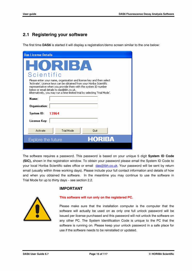
The first time DAS6 is started it will display a registration/demo screen similar to the one below:
The software requires a password. This password is based on your unique 5 digit System ID Code
(SIC), shown in the registration window. To obtain your password please email the System ID Code to
your local Horiba Scientific sales office or email [email protected]. Your password will be sent by return
email (usually within three working days). Please include your full contact information and details of how
and when you obtained the software. In the meantime you may continue to use the software in
Trial Mode for up to thirty days – see section 2.2.
IMPORTANT
This software will run only on the registered PC.
Please make sure that the installation computer is the computer that the
software will actually be used on as only one full unlock password will be
issued per license purchased and this password will not unlock the software on
any other PC. The System Identification Code is unique to the PC that the
software is running on. Please keep your unlock password in a safe place for
use if the software needs to be reinstalled or updated.
User guide DAS6 Fluorescence Decay Analysis Software
DAS6 User Guide 6.7 Page 16 of 117 © HORIBA Scientific
Once you have received the unlock password it should be entered into the License Key box on the
registration screen along with your Name and Organisation.
The "Activate" button should be clicked to activate the software. If the password is correct, the software
will start. On subsequent executions a splash screen will be displayed and the registration window is not
shown again. Please contact your local HORIBA Scientific sales office if you need more information.
2.2. Trial Mode
The trial version will run with all features enabled for 30 days. On subsequent executions the registration
screen will show, but as long as there is time left in the evaluation period the "Trial Mode" button may be
clicked.
After 30 days, the software will cease to work.

User guide DAS6 Fluorescence Decay Analysis Software
DAS6 User Guide 6.7 Page 17 of 117 © HORIBA Scientific
3. The DAS6 Interface
DAS6 software can be started in two ways:
from the Windows Start menu Start Programs HORIBA Scientific DAS6 Analysis
double-clicking any “.DAS” file in a Windows Explorer window
New DAS files can be created by using our DataStation acquisition software (supplied with instruments
from HORIBA Scientific), by importing data files from older v4.2 IBH files or other formats, or by using the
DAS File Creation Utility (DFCU). The creation of DAS files is described in more detail in section 10. For
use with this manual, a number of example .DAS files have been included in the examples folder.
While reading this section, it is recommended that you open file “Exp1.das” by double-clicking its icon.
You will be presented with a display similar to that shown below, which has the main workspace areas
indicated and which will be described below.

User guide DAS6 Fluorescence Decay Analysis Software
DAS6 User Guide 6.7 Page 18 of 117 © HORIBA Scientific
3.1 Workspace Areas
The Information Area contains various details about the data in the currently loaded file; the look of
this area and the information shown changes depending on the type of file loaded (i.e. lifetime,
anisotropy, global or batch). Examples of information displayed are; peak counts and peak
channels, counts within cursor ranges, time calibration and background values.
The “comments” tab allows display of optional information which might have been saved by
DataStation as part of the measurement.
The drop-down list, at the bottom of the information area, allows selection of the fit module. The list
shows only modules appropriate to the files type loaded.
The Data Tree shows a graphical representation of the loaded data file.
The Data and Fit Graph shows:
- the instrumental response (referred to a “prompt”) – blue dots
- the fluorescence response (referred to as “decay”) - red dots
- the fitted function – green line
The Residuals Display shows the deviation, in standard deviations, between the decay and the
fitted function. This section of the screen can also show the autocorrelation function for a fit (see the
description of the autocorrelation tool in section 3.3 below).
The Fit Results Display shows the results for any stored fit selected from the Data Tree. The data
shown here includes information about the data, selected fit algorithm, input parameters to the fit
and the calculated results of the fit. This data can be opened in a resizable window by clicking on the
"Open in Window" text at the top-right of the Fit Results Display.
The Range Panel allows the cursor values (in channels) to be adjusted, the cursors can also be
dragged using the mouse. Generally each measured or intermediate data item in the tree has a low-
high cursor pair associated with it that allow ranges to be defined. Saved fits do not have cursors. At
most two pairs of cursors are visible at any one time -- usually a prompt pair and a decay pair. If two
pairs are visible they can be "tied" so that their values are equal - in this case only the decay pair can
be moved and the prompt pair will follow automatically. Cursor ranges should always be set before
performing a fit calculation.
User guide DAS6 Fluorescence Decay Analysis Software
DAS6 User Guide 6.7 Page 19 of 117 © HORIBA Scientific
3.2 Menus and toolbars
The standard toolbar at the top of the application window is shown here. There are minor changes when
“Batch” and “Global” modules are used and these are described in the corresponding module
description sections.
Most of these toolbar buttons are also contained within the menus and a description of the functionality of each button is described within the menu description below.
There are only four menus: “File”, “Edit” “Tools” and “View” and these closely adhere to standard
windows operation. Note that keyboard shortcuts are available for many menu items and these are
indicated at the right of the menus items.
The “File” menu is shown below.
“New” Creates a new DAS file – this is dealt with in more detail in section 9.
“Open Open an existing DAS file.
“Save As” allows you to save a copy of the file.
“Print Setup” opens the standard windows component for printer selection and set-up. Note that the
printer selected becomes the system’s default printer.

User guide DAS6 Fluorescence Decay Analysis Software
DAS6 User Guide 6.7 Page 20 of 117 © HORIBA Scientific
“Print” will show the Print Setup dialog box to allow selection of printing preferences before
printing begins. The toolbar button will print to the default printer without showing the Print Setup
dialog box.
“Exit” closes DAS6.
The “Edit” menu is shown below.
“Settings” Set the general defaults for folders and files.
“Time Calibration” allows a time calibration value (i.e. nanoseconds/channel) to be entered or edited.
DAS files created by DataStation will most likely already contain a time calibration value. However,
files created using the “New” function might not have a value set.
“Copy to Clipboard” copies information to the clipboard so that it can be pasted into other
applications such as word processors and spreadsheets. It is possible to copy the main decay
graph and the residuals graph or copy the data for the decay graph .
“Export as Text” allows information to be output as a text file. The information written to the file
depends on what is being viewed in the main “Data and Fit Graph” window. If a fit is being viewed,
the fit results and data are written.

User guide DAS6 Fluorescence Decay Analysis Software
DAS6 User Guide 6.7 Page 21 of 117 © HORIBA Scientific
The “Tools” menu is shown below.
“Cursors -> Zoom” set the cursors to match the current zoom range.
“Zoom -> Cursors” set the zoom range to match the current cursors.
“Zoom Full” Zoom the main graph to its full extent (depends on the data range of the loaded
file).
“Pan X” Pan on the X axis of the main graph (click, hold and drag the mouse to pan).
“Zoom X” Zoom on the X axis of the main graph (click, hold and drag the mouse to select a
range).
“Cursor” Switch to cursor mode (you can also double-click anywhere on the graph when in zoom
or pan mode to switch to cursor mode).
“Reverse” Reverse the measured data. This is useful when the data have been measured in
“reverse mode” and the time axis therefore needs to be reversed before the data can be analysed.
This function can only be used if there are no stored results (i.e. no fits have yet been performed).
“Omit Prompt” is used when a tail fit is required in the exponential fits instead of a reconvolution fit.
Normally, if the DAS file contains a prompt and a decay, the exponential fit module would expect to
perform a reconvolution fit. This selection forces the module to ignore the prompt and perform a tail
fit.
“Subtract Background File” allows data in a second DAS file to be subtracted from the current data
and the result to be saved as a new DAS file. This is useful when a “blank” is run for comparison
against a sample measurement. However, this function should be used with caution as it does not
take into consideration the data weights so the integrity of the statistical information in any
User guide DAS6 Fluorescence Decay Analysis Software
DAS6 User Guide 6.7 Page 22 of 117 © HORIBA Scientific
subsequent analysis is lost. The DAS files should have the same structure (i.e. same number of data
points in decays and prompts, if present).
“Swap Prompt/Decay” allows reversal of the prompt and decay data. Sometimes, in error, the
prompt and decay are measured in the wrong order. This selection allows the error to be corrected.
It can only be used if there are no stored results (i.e. no fits have yet been performed or all stored fits
have been deleted).
“Deconvolute Prompt” allows a second exponential decay to be used as a prompt. The function
enables a working prompt for decay analysis to be calculated from the exponential decay
measurement using fast Fourier transforms. This function is described in more detail in the chapter
“When a Prompt Cannot be Measured”
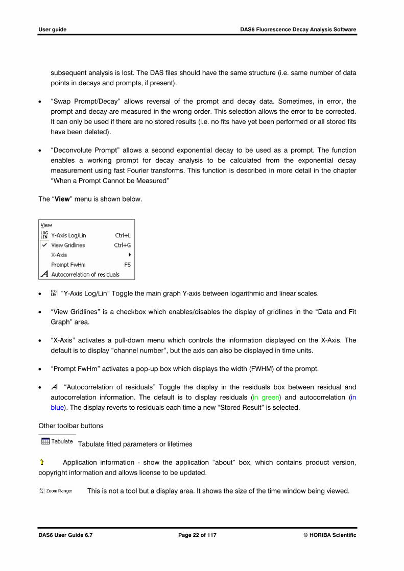
The “View” menu is shown below.
“Y-Axis Log/Lin” Toggle the main graph Y-axis between logarithmic and linear scales.
“View Gridlines” is a checkbox which enables/disables the display of gridlines in the “Data and Fit
Graph” area.
“X-Axis” activates a pull-down menu which controls the information displayed on the X-Axis. The
default is to display “channel number”, but the axis can also be displayed in time units.
“Prompt FwHm” activates a pop-up box which displays the width (FWHM) of the prompt.
“Autocorrelation of residuals” Toggle the display in the residuals box between residual and
autocorrelation information. The default is to display residuals (in green) and autocorrelation (in
blue). The display reverts to residuals each time a new “Stored Result” is selected.
Other toolbar buttons
Tabulate fitted parameters or lifetimes
Application information - show the application “about” box, which contains product version,
copyright information and allows license to be updated.
This is not a tool but a display area. It shows the size of the time window being viewed.
User guide DAS6 Fluorescence Decay Analysis Software
DAS6 User Guide 6.7 Page 23 of 117 © HORIBA Scientific
4. Measurement types and performing a Fit
4.1 Measurement Types
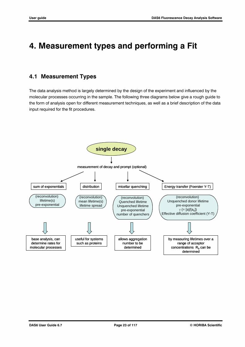
The data analysis method is largely determined by the design of the experiment and influenced by the
molecular processes occurring in the sample. The following three diagrams below give a rough guide to
the form of analysis open for different measurement techniques, as well as a brief description of the data
input required for the fit procedures.
sum of exponentials distribution Energy transfer (Foerster Y-T)micellar quenching
single decay
measurement of decay and prompt (optional)
(reconvolution) lifetime(s)
pre-exponential
(reconvolution)mean lifetime(s)lifetime spread
(reconvolution) Quenched lifetime
Unquenched lifetimepre-exponential
number of quenchers
(reconvolution) Unquenched donor lifetime
pre-exponential (= [a]/[a0])
Effective diffusion coefficient (Y-T)
allows aggregation number to be determined
by measuring lifetimes over a range of acceptor
concentrations R0 can be determined
useful for systems such as proteins
base analysis, can determine rates for
molecular processes
sum of exponentials distribution Energy transfer (Foerster Y-T)micellar quenching
single decay
measurement of decay and prompt (optional)
(reconvolution) lifetime(s)
pre-exponential
(reconvolution) lifetime(s)
pre-exponential
(reconvolution)mean lifetime(s)lifetime spread
(reconvolution)mean lifetime(s)lifetime spread
(reconvolution) Quenched lifetime
Unquenched lifetimepre-exponential
number of quenchers
(reconvolution) Quenched lifetime
Unquenched lifetimepre-exponential
number of quenchers
(reconvolution) Unquenched donor lifetime
pre-exponential (= [a]/[a0])
Effective diffusion coefficient (Y-T)
(reconvolution) Unquenched donor lifetime
pre-exponential (= [a]/[a0])
Effective diffusion coefficient (Y-T)
allows aggregation number to be determined
by measuring lifetimes over a range of acceptor
concentrations R0 can be determined
useful for systems such as proteins
base analysis, can determine rates for
molecular processes

User guide DAS6 Fluorescence Decay Analysis Software
DAS6 User Guide 6.7 Page 24 of 117 © HORIBA Scientific
anisotropy
measurement of decays (VV, VH) and prompt (optional) and g-factor (optional)
rotational correlation timer0, r
Just requires VV, VH and knowledge of g-factortr still has influence of
prompt
Requires impulse response from sum fitand measurement of
prompt. tr does not have
influence of prompt.
Fit to anisotropy function
reconvolutionrotational correlation time
r0, r
Fit to difference of VV and VH decay data
Provides decay parameters.Required if fitting to
difference data.Knowledge of g-factor
needed .
Fit to sum of VV+VH decay data
reconvolutionlifetime(s)
pre-exponential
V – vertical polariserH –horizontal polariser
anisotropy
measurement of decays (VV, VH) and prompt (optional) and g-factor (optional)
rotational correlation timer0, r
rotational correlation timer0, r
Just requires VV, VH and knowledge of g-factortr still has influence of
prompt
Requires impulse response from sum fitand measurement of
prompt. tr does not have
influence of prompt.
Fit to anisotropy function
reconvolutionrotational correlation time
r0, r
reconvolutionrotational correlation time
r0, r
Fit to difference of VV and VH decay data
Provides decay parameters.Required if fitting to
difference data.Knowledge of g-factor
needed .
Fit to sum of VV+VH decay data
reconvolutionlifetime(s)
pre-exponential
reconvolutionlifetime(s)
pre-exponential
V – vertical polariserH –horizontal polariser

User guide DAS6 Fluorescence Decay Analysis Software
DAS6 User Guide 6.7 Page 25 of 117 © HORIBA Scientific
multiple lifetime measurement
microscope mapTRES
single lifetime measurements
multiple decays
measurement of decay and prompt (optional)
batch
(reconvolution) lifetime(s)
pre-exponential same decay model
base analysis, can determine rates for
molecular processesdecays analysed
sequentially
DFCU to combine files
global
assumes common lifetimes for emitting species
allows spectra to be resolved for different species with wavelength (TRES)
(reconvolution) lifetime(s)
pre-exponential linked lifetimes
multiple lifetime measurementmultiple lifetime measurement
microscope mapTRES
single lifetime measurementssingle lifetime measurements
multiple decays
measurement of decay and prompt (optional)
batch
(reconvolution) lifetime(s)
pre-exponential same decay model
base analysis, can determine rates for
molecular processesdecays analysed
sequentially
batch
(reconvolution) lifetime(s)
pre-exponential same decay model
(reconvolution) lifetime(s)
pre-exponential same decay model
base analysis, can determine rates for
molecular processesdecays analysed
sequentially
DFCU to combine files
global
assumes common lifetimes for emitting species
allows spectra to be resolved for different species with wavelength (TRES)
(reconvolution) lifetime(s)
pre-exponential linked lifetimes
global
assumes common lifetimes for emitting species
allows spectra to be resolved for different species with wavelength (TRES)
(reconvolution) lifetime(s)
pre-exponential linked lifetimes
(reconvolution) lifetime(s)
pre-exponential linked lifetimes
User guide DAS6 Fluorescence Decay Analysis Software
DAS6 User Guide 6.7 Page 26 of 117 © HORIBA Scientific
4.2 Performing a Basic Fit
This section is intended as a quick start and covers the most commonly used analysis: exponential
decays with and without the presence of scattered light.
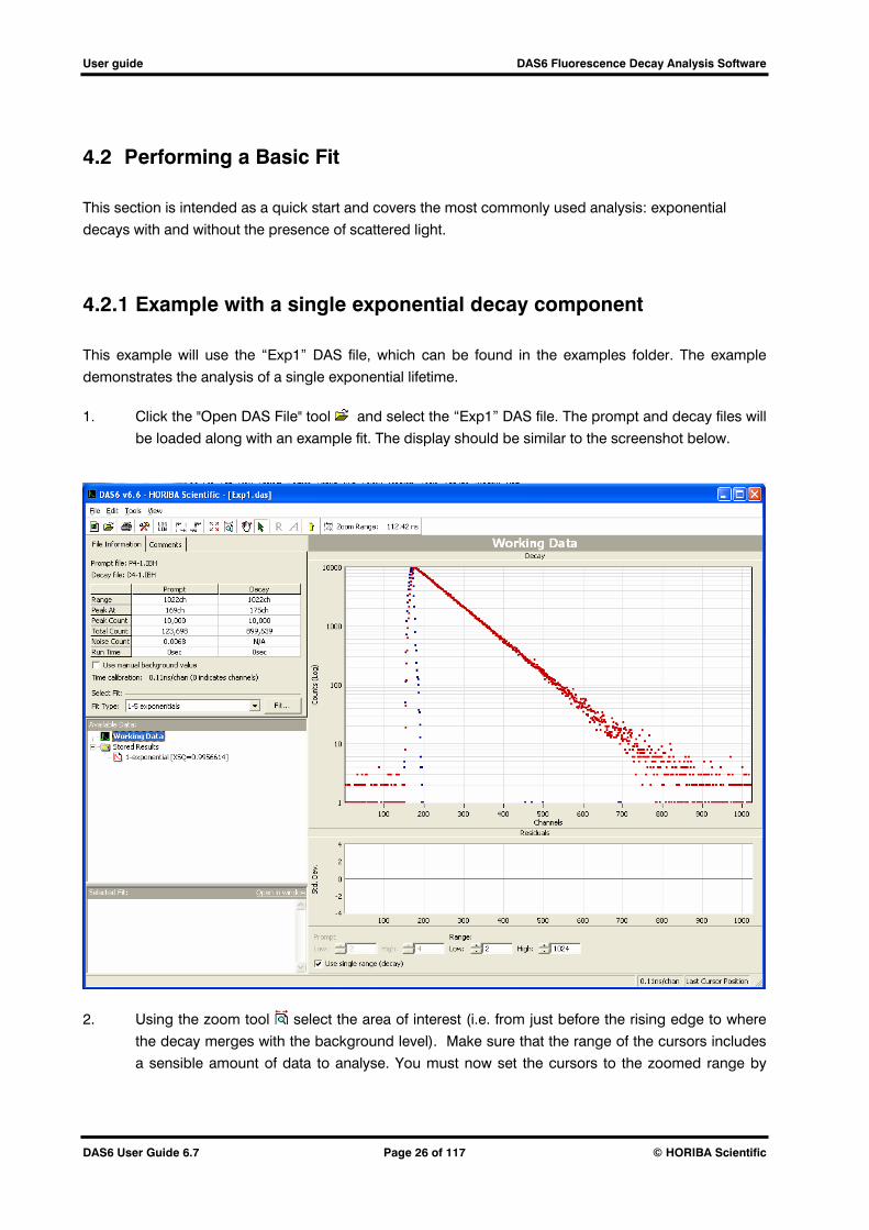
4.2.1 Example with a single exponential decay component
This example will use the “Exp1” DAS file, which can be found in the examples folder. The example
demonstrates the analysis of a single exponential lifetime.
1. Click the "Open DAS File" tool and select the “Exp1” DAS file. The prompt and decay files will
be loaded along with an example fit. The display should be similar to the screenshot below.
2. Using the zoom tool select the area of interest (i.e. from just before the rising edge to where
the decay merges with the background level). Make sure that the range of the cursors includes
a sensible amount of data to analyse. You must now set the cursors to the zoomed range by
User guide DAS6 Fluorescence Decay Analysis Software
DAS6 User Guide 6.7 Page 27 of 117 © HORIBA Scientific
using the “cursor to zoom” tool . You can see the channel information for the zoomed range in
the “Range Panel” below the graphs and also in the “Information Area” to the left of the main
graph. If you make a mistake, zoom out using the tool and start again.
The example fit uses “low” and “high” values of 140 and 900 respectively. These values can be
typed directly into the “Range Panel”, if preferred.
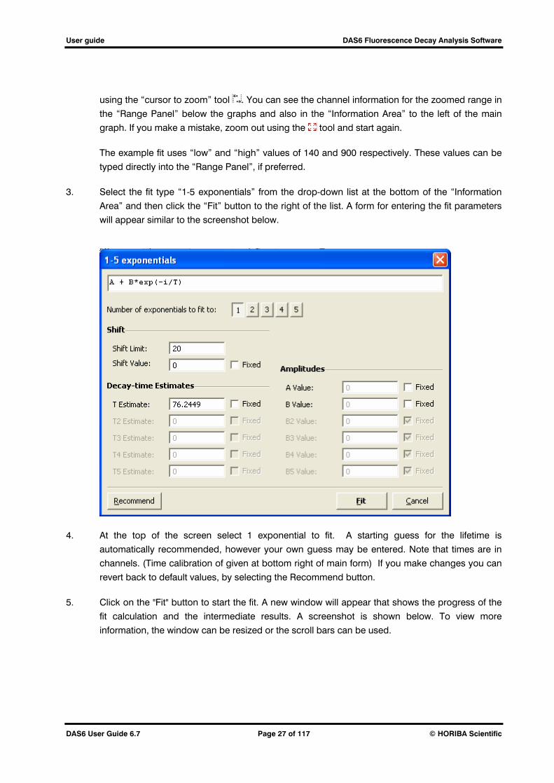
3. Select the fit type “1-5 exponentials” from the drop-down list at the bottom of the “Information
Area” and then click the “Fit” button to the right of the list. A form for entering the fit parameters
will appear similar to the screenshot below.
4. At the top of the screen select 1 exponential to fit. A starting guess for the lifetime is
automatically recommended, however your own guess may be entered. Note that times are in
channels. (Time calibration of given at bottom right of main form) If you make changes you can
revert back to default values, by selecting the Recommend button.
5. Click on the "Fit" button to start the fit. A new window will appear that shows the progress of the
fit calculation and the intermediate results. A screenshot is shown below. To view more
information, the window can be resized or the scroll bars can be used.

User guide DAS6 Fluorescence Decay Analysis Software
DAS6 User Guide 6.7 Page 28 of 117 © HORIBA Scientific
6. When the fit has completed, the final results are shown and the graphs updated to show the
fitted function curve and the residuals. At this point you can choose to discard the results or to
keep them. If you keep the results you will be asked for a name for them and they will then be
stored in the “Data Tree” as “Stored Results” and can be recalled at any time.
This is a very simple example and you should experiment as much as possible to get comfortable with
using your new analysis software. The correct lifetime value is 8.5 nanoseconds.
The DAS file contains all the information for prompt, decay and fits and is automatically saved each time
a new stored fit is added, when a different file is opened and before the application exits. There is no
need to explicitly save the file.
Before continuing, select your fit (by clicking on it in the “Stored Fits” tree) and then click the “Open In
Window” tag at the top right of the “Fit Results Display”. A new window containing the fit results will
open. Close the window after viewing.
This would be a good time to experiment with the “Print”, “Export as Text” and “Copy to Clipboard”
functions.
User guide DAS6 Fluorescence Decay Analysis Software
DAS6 User Guide 6.7 Page 29 of 117 © HORIBA Scientific
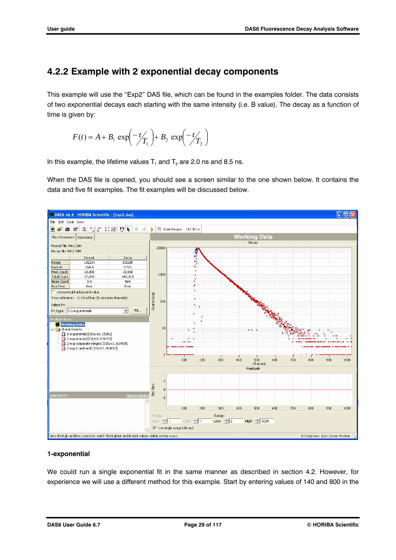
4.2.2 Example with 2 exponential decay components
This example will use the “Exp2” DAS file, which can be found in the examples folder. The data consists
of two exponential decays each starting with the same intensity (i.e. B value). The decay as a function of
time is given by:
22
11 expexp)( T
tBTtBAtF
In this example, the lifetime values T1 and T2 are 2.0 ns and 8.5 ns.
When the DAS file is opened, you should see a screen similar to the one shown below. It contains the
data and five fit examples. The fit examples will be discussed below.
1-exponential
We could run a single exponential fit in the same manner as described in section 4.2. However, for
experience we will use a different method for this example. Start by entering values of 140 and 800 in the

User guide DAS6 Fluorescence Decay Analysis Software
DAS6 User Guide 6.7 Page 30 of 117 © HORIBA Scientific
“Range Low” and “Range High” boxes then click on the main window. You will see that the high and low
cursors have moved to the specified positions. Next, click “Fit” to get the parameters window and run the
fit by clicking “Recommend” then “Fit”. You have just reproduced the first fit in the “Stored Results” tree
and can either “Keep” or “Discard” it.
Now highlight the “1-exponential” fit in the “Stored Results” tree. The main plot, residuals plot and 2
(XSQ) value all indicate a poor fit:
Main plot – fitted function clearly differs in places from measured data.
Residuals plot – for a good fit, these should be randomly distributed around zero and within the
range of a few standard deviations.
2 value – for a good fit this should be near to 1.0 (<1.2 is usually ok provided the residuals are
random).
Click “Open in Window” to view the results - The lifetime value of 7.2 ns has little credibility in this case.
2-exponential
We will now repeat the process and fit to a two exponential decay model. Click on “Working Data” and
then check that the range is still set at channels 140 to 800. Then click on “Fit”, select “2” as the number
of exponentials and click “Recommend” to get starting guesses. The parameters window should look
similar to the one below.

User guide DAS6 Fluorescence Decay Analysis Software
DAS6 User Guide 6.7 Page 31 of 117 © HORIBA Scientific
Click “Fit” to complete the process. You have just reproduced the second fit and can either “Keep” or
“Discard”.
Now highlight the “2-exponential” fit” in the “Stored Results” tree. The main plot, residuals plot and 2
(XSQ) value all indicate a good fit.
Main plot – fitted function closely follows the measured data.
Residuals plot – the residuals appear to be randomly distributed around zero and all are within
the range of a few standard deviations.
2 value – the value is near to 1.0 (i.e. <1.2).
Click “Open In Window” to view the results - The lifetime values of 1.92 ns and 8.46.ns are in good
agreement with those expected. Also, we were expecting equal B values and you will see that these are
in reasonable agreement.
This is a good point at which to explain the [Rel.Ampl.] (relative amplitude) figures displayed alongside
the B1 and B2 values. If we have a 1 ns and a 2 ns lifetime starting at the same intensity, we will see
more photons from the 2 ns decay because it emits for longer. The actual number of photons is
proportional to “B” multiplied by “T”. The relative amplitudes are therefore the percentage of photons
coming from the different decays,
It will be evident that, if the decays are from different chromophores, this is the ratio of the photons
coming from each.
In the present example we expect to see 19% of photons from the 2 ns decay and 81% from the 8.5 ns
decay, which is in close agreement with the fit.
2-exp (separate ranges)
Although it is very quick and easy to perform the above fits, they assume that there is meaningful data
throughout the same ranges of the prompt and decay. However, in this example, the “Prompt” has
nothing but noise in channels above 200 and these are best discarded.
Click on “Working Data” then un-check the “Use single range” box in the “Range Panel”. You can now
enter separate range values for prompt and decay. Enter values of 150 to 200 for the prompt, and 140 to
800 for the decay.
If you now run a two exponential fit, you should obtain the results for the fourth example.
Again, the values are all good.
iiii TBTB

User guide DAS6 Fluorescence Decay Analysis Software
DAS6 User Guide 6.7 Page 32 of 117 © HORIBA Scientific
2-exp (combined)
In this example, separate ranges are used for the prompt and decay. Also, the A value is fixed. Again, the
values are all good.
You will see from the five fits in this section that there are some subtle effects associated with fixing vales
and selecting data ranges. This is something that you should experiment with. Scientifically, it is always
best to separate the ranges and to fix whatever values can sensibly be fixed. However, a great deal of
valid, preliminary investigation can be performed quickly and reliably by letting the default settings do
the work and hence avoiding the extra effort involved.
4.2.3 Example with scattered light
This example will use the “Exp2Scatter” DAS file, which can be found in the examples folder. The data
consists of two exponential decays each starting with the same intensity (i.e. B value) but in this example
there is an additional, significant scattered light component. As in section 4.2, the lifetime values are 2.0
ns and 8.5 ns.
After working through the examples in sections 4.1 and 4.2, you should now be familiar with running
simple exponential fits. This section therefore simply describes the fits included in the file. You can
repeat the analyses for yourself using the starting conditions that you will find in the in the “Stored
Results”.
When the DAS file is opened, you should see a screen similar to the one shown below. It contains the
data and four fit examples. The examples will be discussed below.

User guide DAS6 Fluorescence Decay Analysis Software
DAS6 User Guide 6.7 Page 33 of 117 © HORIBA Scientific
1-exp
This is simply the fit to a single exponential decay model. Looking at the residuals, this is clearly not the
correct decay model. This fit has been included for comparison with the ones below it.
2-exp
Again, this is clearly not the correct decay model. However, looking at the residuals, it is a much closer fit
than the single exponential decay model. In fact, the residuals are a very good guide as to whether there
is more information available or not.
Looking at the residuals, you can see that there is more information present because they are not
randomly distributed around zero.
3-exp
Here is where the situation gets interesting. You can think of scattered light as a delta function or as a
very fast decay component. If you examine the “Stored Results” for the “3-exp” fit, you will see that this
decay model has found lifetimes of 1.9 ns, 8.4 ns and 13.1 ps. The last value is, of course, due to
scattered light.

User guide DAS6 Fluorescence Decay Analysis Software
DAS6 User Guide 6.7 Page 34 of 117 © HORIBA Scientific
Although the fit to a three exponential model was successful in this case, it is not always successful and
sometimes the fit fails as the lifetime value gets shorter and shorter. A safer way to deal with scattered
light is to deliberately fix one of the lifetime components at a fast value. It is usually recommended to fix
T1 at a value of 0.5 channels.
2-exp plus scatter
The final fit in the set shows the situation when T1 is deliberately fixed at 0.5 channels. In this case the
parameter input screen is similar to the one shown below.
Examining the lifetime values and B values found by the fit, you will see that it has found reasonable
values for both lifetimes and intensities.
User guide DAS6 Fluorescence Decay Analysis Software
DAS6 User Guide 6.7 Page 35 of 117 © HORIBA Scientific
4.3 Interpreting the results of the analysis
The meaning of the parameters recovered from the DAS6 analysis will depend on the sample application. Generally speaking DAS6 will return the following parameters (although it is strongly advised to see the specific section related to the required decay model for other recovered parameters)
A value = background offset
B value = pre-exponential function which relates to how much of an emitting species there is.
T value = lifetime
The magnitude of the B values returned in the fit are dependent on whether or not reconvolution is used in fitting the data. Without reconvolution the values are in counts and can easily be linked to the peak number of counts (ie for a single exponential its magnitude should be ~ the count value in the start channel). The value after reconvolution is not in counts, but still reflects the amount of a particular emitting species.
There are two main ways in which the B values are represented
i. As a relative amplitude (Rel. Ampl.), in which the pre-exponential is weighted by the lifetime, this is useful when comparing with steady state spectra
ii. By normalising (B) values, this is useful when performing in depth analysis on multi-component systems.
If we consider the decay to be represented as a sum of exponential components
Then the relative amplitude (fractional) is
while the normalised pre-exponential value is
The former weights the “amount” of an emitting species by the lifetime and allows a more direct comparison with steady state data, while the latter provides information concerning the relative concentrations of emitting species. DAS6 gives both of these values, as well as the “raw” B value.
)/exp()( i
n
ii TtBtI
n
ii
ii
B
BB
1
i i
ii
TB
TBf

User guide DAS6 Fluorescence Decay Analysis Software
DAS6 User Guide 6.7 Page 36 of 117 © HORIBA Scientific
It should be noted that the T values (lifetimes) can also be interpreted as rates (k =1/T). Sometimes when comparing results it is helpful to make use of an average lifetime. This can be calculated in two main ways, depending on the application of the result. These can be found in the paper by A. Sillen and Y. Engelborghs. Photochem. 67, 475-486 (1998). To summarise, for most applications the average lifetime can be calculated as the simple sum of normalised pre-exponential multiplied by the lifetime.
This is the output of the average lifetime given by DAS6. Alternatively (for example for use in Stern-Volmer analysis) it can be obtained from
DAS6 provides errors for these recovered values, as indicated by the standard deviation. In practice it is normal to use three standard deviations for the error on a given value.
In order to tell if the fitting model gives a good fit to the measured data the reduced chi-squared (sometimes written as 2 or XSQ) is used. This is probably best employed in conjunction with the weighted residuals to evaluate the goodness of fit.
4.3.1 How do I know if I have a good data fit?
The usual criteria to assess whether a fit is satisfactory is to use the reduced chi-squared value and to see if there are any trends in the weighed residuals. Also the fitting of an additional exponential decay component should not produce any significant improvement. The returned values should also be sensible. Generally, when using reconvolution, the shortest measurable lifetime that can be returned is approximately 10 times less than the instrumental full width at half maximum. The following should be considered in assessing the fit data, along with any prior knowledge of the system studied.
Chi-squared value below 1.2, not meaningfully improved by adding an extra decay component.
Randomly distributed weighted residuals are expected for a good fit.
Do the lifetime(s) correspond to previous reports (measurements or literature)?
Lifetime values of 10-11 seconds (0.01 ns) or less than one data channel should be treated with caution and may relate to scattered excitation light reaching the detector.
Large (e.g. more than ~3 channels) or negative shifts may indicate a problem depending on the detector and wavelengths used.
Excessive errors (s. dev) on the data.
n
iiiave TB
1
n
iii
i
n
ii
ave
TB
TB
1
2
1

User guide DAS6 Fluorescence Decay Analysis Software
DAS6 User Guide 6.7 Page 37 of 117 © HORIBA Scientific
Negative pre-exponential components (B values) are not necessarily a sign of a bad fit, they can indicate the presence of an excited state process and are referred to as “rise times”.
General process for lifetime analysis:
A good fit is determined by examining the 2 and residuals and using any prior knowledge of the system. Check the size of the residuals and whether they are random, check if adding another exponential reduces the value of 2.
Good fit
Bad fit
Open data file
Select fit range
Open data file
Select fit range
Fit monoexponential
Open data file
Select fit range
Open data file Open data file
Select fit range
Open data file
Select fit range
Open data file
Fit monoexponential
Select fit range
Open data file
Add exponential and refit
Exit Check 2 and residuals

User guide DAS6 Fluorescence Decay Analysis Software
DAS6 User Guide 6.7 Page 38 of 117 © HORIBA Scientific
5. Decay Analysis Modules
Each of the DAS6 modules provides functionality for a different fitting function (or family of functions).
5.1 Exponential Fits
Exponential fits have already been used as a training example in section 4. This section deals with an
example containing five exponential decay components. The decay model is given by:
55
44
33
22
11 expexpexpexpexp)( T
tBTtBT
tBTtBT
tBAtF
The example file is “Exp5”, and the opening screen is shown below.

User guide DAS6 Fluorescence Decay Analysis Software
DAS6 User Guide 6.7 Page 39 of 117 © HORIBA Scientific
The data in this file contains five exponential decay components with equal B vales. The lifetimes are 2.0,
4.0, 8.0, 16.0 and 32.0 nanoseconds respectively. It should be noted that the data is collected to 50,000
counts in the peak, which is significantly higher than the 10,000 counts used in previous examples. Also
note that the data are collected into 4095 channels (time window of 450 ns) compared to the previous
examples which were collected into 1024 channels (time window of 112 nanoseconds).
In practice this means that it will have taken 20 times longer to perform the measurement. The reason
that this extra information is needed will become evident from the data analysed below. However, it is
intuitively obvious that more complicated models require more data (i.e. more photons/counts) than
simple models.
The example file contains five fits. In all five cases, separate prompt and decay ranges were used. For
the prompt the range used was 150 – 200 channels and for the decay the range was 140 – 3500
channels.
1-exp
Clearly, a one exponential decay model is incorrect.
2-exp
Clearly, a two exponential decay model is incorrect and the residuals show that more information is
available.
3-exp
This is really quite a good fit and, looking at the residuals, there is little evidence for trying anything more
complicated. However, we know that this data contains five decay components. So, however good the
fit, the lifetime values are meaningless. This illustrates two very important points:
Just because the model gives a good fit, it does not prove it is the
correct model. There has to be an independent reason to believe
the model is appropriate. This generally comes from careful
planning of a series of measurements to test a hypothesis. Don’t
be tempted to measure today and interpret tomorrow!
With three exponentials, you can fit just about any TCSPC data!
It is tempting, from the above, to conclude that more complicated models cannot be studied by this
technique. Fortunately that is not the case. The fit above allowed all values to be varied. However, if there
is prior knowledge of some of the decay components either from a different measurement or even a
different technique, then some lifetime values can be fixed.

User guide DAS6 Fluorescence Decay Analysis Software
DAS6 User Guide 6.7 Page 40 of 117 © HORIBA Scientific
5-exp (2 fixed)
This fit example illustrates the point made above. Two of the values are “fixed” and reasonable starting
guesses have been made for the other three lifetimes. The parameter input screen for this is shown
below.
You can see that T1 and T2 have all been “Fixed”. If you check the fit results you will see that the fit has
found the following values:
T1 = 2.0 ns (fixed)
T2 = 4.0 ns (fixed)
T3 = 8.6 ns (expected value of 8.0 ns)
T4 = 17.1 ns (expected value of 16.0 ns)
T5 = 32.1 ns (expected value of 32.0 ns)
The agreement, which is reasonable, is an indication that fixing parameters can yield some useful
results.
User guide DAS6 Fluorescence Decay Analysis Software
DAS6 User Guide 6.7 Page 41 of 117 © HORIBA Scientific
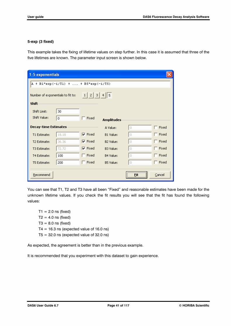
5-exp (3 fixed)
This example takes the fixing of lifetime values on step further. In this case it is assumed that three of the
five lifetimes are known. The parameter input screen is shown below.
You can see that T1, T2 and T3 have all been “Fixed” and reasonable estimates have been made for the
unknown lifetime values. If you check the fit results you will see that the fit has found the following
values:
T1 = 2.0 ns (fixed)
T2 = 4.0 ns (fixed)
T3 = 8.0 ns (fixed)
T4 = 16.3 ns (expected value of 16.0 ns)
T5 = 32.0 ns (expected value of 32.0 ns)
As expected, the agreement is better than in the previous example.
It is recommended that you experiment with this dataset to gain experience.

User guide DAS6 Fluorescence Decay Analysis Software
DAS6 User Guide 6.7 Page 42 of 117 © HORIBA Scientific
5.2 Exciplex
The exciplex decay model is given by:
21expexp)( T
tT
tBAtF
The example file is “Exciplex”, and the opening screen is shown below.
This is an example with lifetime values of 8.5 ns and 2.0 ns for T1 and T2 respectively. It is interesting to
note the distinct rise time on the data. Also, it is mathematically evident that in this case T1 must always
be greater than T2 (the lifetime associated with the negative pre-exponential –“rise time”).
The example file contains only one “Stored Result” and the parameter input screen, obtained by
selecting “Exciplex” as the fit type, is shown below.

User guide DAS6 Fluorescence Decay Analysis Software
DAS6 User Guide 6.7 Page 43 of 117 © HORIBA Scientific
Examination of the fit results shows lifetime values of 8.4 ns and 2.0 ns, which are in good agreement
with the values expected.

User guide DAS6 Fluorescence Decay Analysis Software
DAS6 User Guide 6.7 Page 44 of 117 © HORIBA Scientific
5.3 Fit to Exponential Series
This module simply allows fits to be performed for up to 30 fixed lifetimes. Reconvolution is performed, but no shift. The fitted function is of the form:
3030
22
11 exp...expexp)( T
iBTiBT
iBAtF .
The main purpose of this module is to parameterise otherwise difficult data so that an impulse response function can be calculated (i.e. so that a smooth curve representing the deconvoluted data can be extracted).
The example file is “ExpSeries”, and the opening screen is shown below
The example data is a mixture of seven decays of equal initial intensity (i.e. equal B values) with lifetime values of 10, 20, 30, 40, 50, 60, and 70 channels. (Note that this example is working in channels rather than nanoseconds).

User guide DAS6 Fluorescence Decay Analysis Software
DAS6 User Guide 6.7 Page 45 of 117 © HORIBA Scientific
There are four fits in the “Stored Results” tree.
1-exponential 2-exponential 3-exponential
These are included for general interest and to illustrate the point that most data can be fitted to a three exponential model (see section 5.1).
Series
This example uses the “Fit to exponential series” module to parameterise the data. A data range of channels 140 to 800 has been selected and the parameter input screen is shown below.
In this example we have fitted to a series of 5 exponentials and the fixed lifetime values can be seen on the parameter input screen above. The fit results can be viewed in the results window by clicking on the ‘series’ entry in the tree view.

User guide DAS6 Fluorescence Decay Analysis Software
DAS6 User Guide 6.7 Page 46 of 117 © HORIBA Scientific
5.4 Förster Quenching
This is an energy transfer model based on dipole-dipole interaction and is described extensively in the
scientific literature (see, for example, J.B. Birks, Photophysics of Aromatic Molecules, 567-576, Wiley,
1970). The Förster approximation assumes the sample under test has sufficiently high solvent viscosity,
that the diffusion length is small compared with the critical transfer distance. Molecules therefore
effectively remain stationary during the energy transfer process. Rapid Brownian rotation is assumed, so
that the orientation factor is replaced by its average value. The decay function is:
22
21
111 exp2exp)( T
tBTt
TtBAtF
Where
23-
0
0
2
1
1010with ,
e)(mole/litrion concentratacceptor Critical
e)(mole/litrion concentratAcceptor
component additional (optional) of Decay time
lifetimedonor d Unquenche
aa
a
a
T
T
This means that in an experiment varying acceptor concentration, we can use a plot of vs a to
determine Ro, the distance at which energy transfer is 50% efficient.
The above equation is, in fact, a 3-dimensional Förster model. DAS6 also allows fitting to a 2-dimensional
model given by:
22
31
111 exp2exp T
tBTt
TtBA
DAS6 can adjust all of the parameters of the model, or accept constraints. One possible constraint is T1,
since it should be known in many instances. Remember that sensible constraints lead to greater stability
in the fitted parameters, often making the difference between curve fitting and kinetic sense.
The example file for this module is “Quenching”, which uses a donor lifetime of 5 ns and a value of 0.3.
The example does not include an optional decay component. Data channels from 140 to 600 were
included in the analysis and the parameter input screen is shown below.

User guide DAS6 Fluorescence Decay Analysis Software
DAS6 User Guide 6.7 Page 47 of 117 © HORIBA Scientific
The resulting fit is shown below.

User guide DAS6 Fluorescence Decay Analysis Software
DAS6 User Guide 6.7 Page 48 of 117 © HORIBA Scientific
5.5 Yokota-Tanimoto Quenching
The Yokota-Tanimoto theory extends the Förster model by taking into account molecular diffusion during
the energy transfer process (see M Yokota and O Tanimoto, J. Phys. Soc. Japan, 22, 779–784, (1967); J
B Birks, “Photophysics of Aromatic Molecules”, Wiley Interscience, 1970, 576 – 580). The decay law is:
22
21
111 exp)(2exp)( T
tBTttCT
tBAtF
Where:
T1 = Unquenched lifetime
T2 = decay time of (optional) additional component
A = Acceptor concentration (mole/litre)
A0 = Critical acceptor concentration (mole/litre)
= A / A0
C(x) = [(1 + 10.87x + 15.5x2) / (1 + 8.734x)]3/4 with x = (Km .R0
6)-1/3 .t2/3 . D*
D* = Effective diffusion coefficient (cm2/ch)
10-28 <= D* <= 1; 0 <= [iY] <= 10 and 0 <= [iY]0 <= 10
Note that the program requires times and time related parameters to be in terms of channels. In particular, the effective diffusion coefficient is required in units of cm2/ch. This is calculated from the more usual units of cm2/sec as follows:
Take D* = 1.9 * 10-5 cm2/sec, say and CAL = 0.35 ns/ch, say then D* = (1.9 * 10-5) * (0.35 * 10-9) cm2/ch ie D* = 6.65 * 10-15 cm2/ch
The parameter input screen is shown below.

User guide DAS6 Fluorescence Decay Analysis Software
DAS6 User Guide 6.7 Page 49 of 117 © HORIBA Scientific
User guide DAS6 Fluorescence Decay Analysis Software
DAS6 User Guide 6.7 Page 50 of 117 © HORIBA Scientific
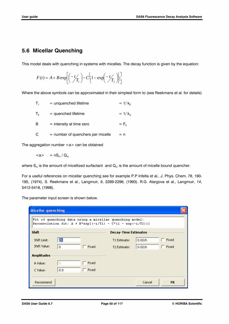
5.6 Micellar Quenching
This model deals with quenching in systems with micelles. The decay function is given by the equation:
21exp1exp)( T
tCTtBAtF
Where the above symbols can be approximated in their simplest form to (see Reekmans et al. for details)
T1 = unquenched lifetime = 1/ k0
T2 = quenched lifetime = 1/ kq
B = intensity at time zero = F0
C = number of quenchers per micelle = n
The aggregation number <a> can be obtained
<a> = nSm / Qm
where Sm is the amount of micellized surfactant and Qm is the amount of micelle bound quencher.
For a useful references on micellar quenching see for example P.P Infelta et al., J. Phys. Chem. 78, 190-
195, (1974), S. Reekmans et al., Langmuir, 9, 2289-2296, (1993). R.G. Alargova et al., Langmuir, 14,
5412-5418, (1998).
The parameter input screen is shown below.
User guide DAS6 Fluorescence Decay Analysis Software
DAS6 User Guide 6.7 Page 51 of 117 © HORIBA Scientific
5.7 Lifetime Distribution
In many physical situations, the fluorophores under investigation can be in diverse local environments,
each affecting the fluorescence lifetime to a slightly different degree. Rather than characterising the
resulting complex decay with more and more exponential components, it can be argued that it is more
realistic to describe such kinetics in terms of a distribution of decay components, whose decay times are
distributed according to an assumed distribution function. The fitted parameters then reduce to two: a
mean decay time and a measure of the width of the associated distribution function.
Two methods are available for performing lifetime distribution analysis. The first method employs a Top
Hat distribution function which allows only a single lifetime distribution to be fitted and the second is the
Non-Extensive Decay Distribution which allows up to five lifetime distributions to be modelled.
5.7.1 Top hat distribution
It is a point of academic discussion whether it is physically more realistic to consider distributed decay
times or distributed decay rates. The arguments tend to favour decay rates. This is fortunate, since the
integrals involved in deriving the decay laws cannot be solved in closed form with the decay time
formulation. The distributed decay law in terms of decay rates can be written as:
dkktkDtkF mmmm
0
exp,,,
where
functionon distributi theofdeviation standard
ratedecay mean
ratedecay
functionon distributi theis ,
lawdecay theis ,,
m
m
mm
mm
k
k
kD
tkF
Ideally, one would like to use a distribution function derived ab initio from the physical mechanisms
responsible for the spread of decay rates. In the absence of such detailed analysis, one might chose a
reasonably behaved function, such as top-hat (rectangular), triangular, Gaussian, Lorentzian, gamma,
etc.
It is important to avoid physically meaningless negative values of k in the distribution integral above.
Distribution functions which fall asymptotically to zero with decreasing (k-km) therefore present a cut-off
problem. This is most serious with the Lorentzian distribution function, because it tends to zero very
slowly, as (|k-km|)-1. The cut-off problem is avoided with the gamma function, since this is defined for

User guide DAS6 Fluorescence Decay Analysis Software
DAS6 User Guide 6.7 Page 52 of 117 © HORIBA Scientific
positive arguments only. The geometric distribution functions (top-hat, triangular) also avoid the
problem, since they go to zero in a well defined manner.
In practice, the form of the resultant decay law does not depend strongly upon the form of the
distribution function. Unimolecular kinetics in a homogenous environment gives a single exponential
decay; a straight line in a semi-logarithmic display. A distribution of decay rates causes this straight line
to bend, with a gradient that decreases monotonically with time. A distribution which tends towards zero
slowly, such as the Lorentzian, will yield a lower fitted width, m , for a given amount of bend than one
with a sharp cut-off, such as the top-hat. However, both will bend and if one fits well, then so, in general,
will the other (provided that cut-off problems at k=0 can be avoided). In our experience, the detailed
forms of the decay functions are insufficiently different to discriminate between them on the basis of
measurements and curve fitting.
For these reasons, we have selected the top-hat distribution function as the basis for our fitting model. In
this case, if the full width of the top-hat function is 2∆, then,
otherwise
kkkkD mmm
0
2, 1
then
ttttktk
tktkf
dkkttkf
mm
mm
k
k
m
m
m
coshsinh1exp
,,
exp2
1,,
2
,mkD
12
0mk k

User guide DAS6 Fluorescence Decay Analysis Software
DAS6 User Guide 6.7 Page 53 of 117 © HORIBA Scientific
The parameters used in the fit model are the mean decay time, Tm, and fractional spread, dTm/Tm, rather
than km, ∆. The use of time, rather than rate variables was decided on the basis of convenience and
consistency with the other FIT programs. The internal working of the module uses the rate variables
defined above. Input and output parameters are converted as follows:
m
m
kTmdTm
kTm
1
Note also that the width parameter used is ∆, the half width at half height, because we thought it easier
to visualise than m , the standard deviation. The relationship between the two quantities is m*3 .
The limiting width, where negative decay rates begin to be included in the distribution is therefore
dTm/Tm = 1. The fitting procedure stops, with an appropriate error message, if this condition is
encountered.
The first example file is “DistExp1”, and the mean lifetime is 5.0 ns with a spread of 1.0 ns (i.e. 20%). The
decay in the opening screen is shown below.
The “Stored Results” shows two examples of fits.

User guide DAS6 Fluorescence Decay Analysis Software
DAS6 User Guide 6.7 Page 54 of 117 © HORIBA Scientific
1-exponential
The analysis to a single exponential decay model was performed over channels 140 to 600 and the
fit to the model is really quite a good fit.
The lifetime value of 5.06 ns is reasonable.
The value 2 of 1.15 is good.
At first glance, the residuals appear to be reasonably random.
However, the residuals are not truly random. On closer inspection a slight oscillation can be seen.
This can also be seen when the autocorrelation is viewed by selecting the tool.
distribution
In this case, the distribution decay model has been selected. The data has a 5 ns decay with a
spread of 20%, and the program finds a decay of 5.02 with a spread of 17.3%. Note also that the
autocorrelation is random.
The second example file is “DistExpTopHat”, and the mean lifetime is 5 ns with a spread of 2.5 ns. The
decay in the opening screen is shown below. You should immediately notice that this decay shows more
curvature than the data in the previous example.

User guide DAS6 Fluorescence Decay Analysis Software
DAS6 User Guide 6.7 Page 55 of 117 © HORIBA Scientific
Again, the “Stored Results” shows two examples of fits.
1-exponential
In this case, the fit is clearly poor.
distribution
In this case, the distribution decay model has been selected. The data has a 5 ns decay with a
spread of 50%, and the program finds a decay of 5.02 with a spread of 48.7%.
The first example illustrates that it really needs a significant spread in lifetimes for the effect of the
distribution to be observed. For 1024 channels of data, with 10,000 counts in the peak, the lower
detection limit is likely to be around 20%. The second example demonstrates that, for wider distributions,
the reliability of the fit is really very good. Of course, the detection limit can be pushed lower by using
more data channels and counting to a higher peak (i.e. by counting more photons).
5.7.2 Non-Extensive Decay Distribution
The non-extensive decay distribution module in the DAS6 data analysis software allows decay data to be
fitted using techniques based on Tsallis non-extensive statistics [C. Tallis, Braz. J. Phys. 39 (2009) 337].
This approach was initially applied to interpret time-resolved fluorescence decays by Włodarczyk [J.

User guide DAS6 Fluorescence Decay Analysis Software
DAS6 User Guide 6.7 Page 56 of 117 © HORIBA Scientific
Włodarczyk, B. Kierdazuk, , Biophys. J. 85 (2003) 58], with a recent application to model time-resolved
decays given by Rolinski and Birch [O.J. Rolinski, D.J.S. Birch. J. Chem. Phys. 129 (2008) 144507].
This method allows more than one lifetime distribution to be modelled and the results can be displayed
graphically.
The following power-like model is used to extract the lifetime distributions from the data
kq
kkkk tqBAtF
115
1
11)( ,
where k is the mean value of the lifetime distribution and q is a parameter of heterogeneity defined by
2
2
12
1
Nq ,
q describes the fluctuation according to the mean value of the decay rate 1 , which is also
indicative of the width of the distribution and the number of decay channels (N). It is worth noting that
the components of F(t) become exponentials as qk tends towards one
kkk etq qqkk
1
11111
.
The analysis software places limits on the values of q ( 3.101.1 q ), the lower limit representing
1q and the upper limit allows the mean value of F(t) to be well defined. When q =1.01 then the
lifetime is tending towards a simple exponential term. When q=1.3 then the distribution of lifetimes is
significantly large.
The results of this analysis are shown graphically with the lifetime distribution for each component
plotted using the gamma function
1
1exp
1
1
1
1
1
1),;(
1
2
qqq
q
qgq
q
,

User guide DAS6 Fluorescence Decay Analysis Software
DAS6 User Guide 6.7 Page 57 of 117 © HORIBA Scientific
with the area under the distribution normalised by the pre-exponential (B value) of the particular
distribution component.
The parameter input screen has the same format as the exponential fit and is shown below
From here it is possible to select the number of lifetime components to fit. Decay time estimates are automatically calculated, but these can be set by the user. Pressing the “Recommend” button will reset the lifetime estimates back to the automatically calculated values. It is possible to fix the amplitude and decay time estimates preventing them being varied during fitting. When the initial estimates have been selected the “Fit” button should be selected to perform the fit.
The distribution fit first calculates an estimate of the lifetimes (T) and amplitudes (B) without the q parameter, it then fine tunes these values and allows q to vary in order to achieve the minimum chi-squared value and optimum fit.
User guide DAS6 Fluorescence Decay Analysis Software
DAS6 User Guide 6.7 Page 58 of 117 © HORIBA Scientific
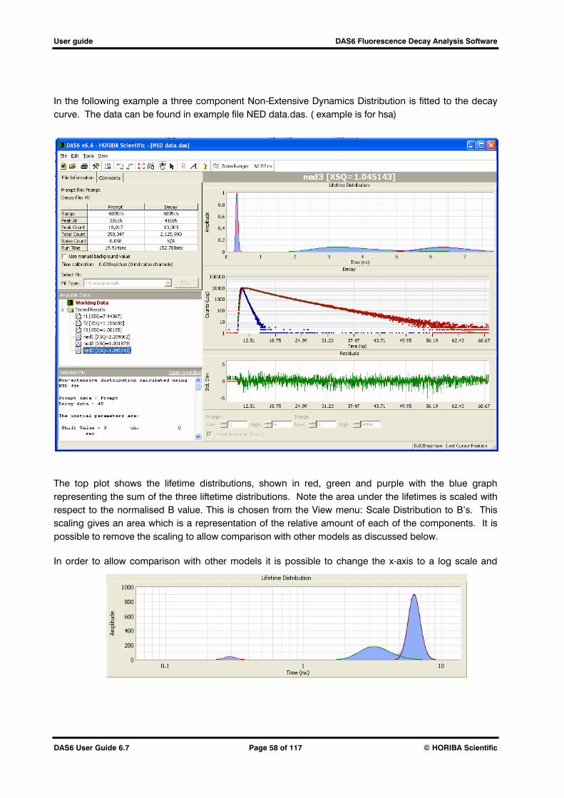
In the following example a three component Non-Extensive Dynamics Distribution is fitted to the decay curve. The data can be found in example file NED data.das. ( example is for hsa)
The top plot shows the lifetime distributions, shown in red, green and purple with the blue graph representing the sum of the three liftetime distributions. Note the area under the lifetimes is scaled with respect to the normalised B value. This is chosen from the View menu: Scale Distribution to B’s. This scaling gives an area which is a representation of the relative amount of each of the components. It is possible to remove the scaling to allow comparison with other models as discussed below.
In order to allow comparison with other models it is possible to change the x-axis to a log scale and

User guide DAS6 Fluorescence Decay Analysis Software
DAS6 User Guide 6.7 Page 59 of 117 © HORIBA Scientific
display the lifetime distributions without scaling to the B values. This can be done using the View menu and the result for the above example is show here.
The middle graph gives the measured data (red dots) with the fitted curve (green line) and the bottom plot shows the standard deviation between the actual and fitted model.
It is possible to view the detailed analysis in the results window or view in a separate window by selecting ‘Open in Window’. The results for the above fit are as follows
In this case the Chi-squared value appears to give a good fit and the standard deviation graph appears to provide random residuals. The relative amplitudes of the three components are given which gives an indication of the contribution of each component to the model. The lifetimes and Q values are displayed along with an estimate of their standard deviation.
The full width half maximum (FWHM) value for each of the lifetime distributions is also given this gives a measure of the spread of the distribution. As the gamma function is asymmetric the calculated lifetimes may not appear at the peak of the distribution curve thus, the Modal Lifetime, which corresponds to the peak of the distribution is also displayed.

User guide DAS6 Fluorescence Decay Analysis Software
DAS6 User Guide 6.7 Page 60 of 117 © HORIBA Scientific

User guide DAS6 Fluorescence Decay Analysis Software
DAS6 User Guide 6.7 Page 61 of 117 © HORIBA Scientific
6. Anisotropy Analysis Module
6.1 Starting an Anisotropy Analysis
This section describes how to get started using an anisotropy file produced by DataStation. For files
created using the “New/Anisotropy” template, see section 10. On first opening an anisotropy file, the
following window is displayed.
Generation of the sum, difference and anisotropy intermediate data (see Appendix B) requires the
measured data Yvv(i) and Yvh(i) to be combined. However, if there is background noise, this needs to be
subtracted before the curves are combined. To obtain a good analysis of anisotropy data, it is important
to set the background values correctly since this affects all subsequent operation on the data.
As can be seen from the screenshot above, there are three ways to set the background. The first way is
easy, automatic and is adequate in most circumstances. The other options require more user
intervention (and thought) but allow more flexibility. The example file “Anisotropy.DAS” has already been
loaded, so the above message does not appear: it can be viewed using the “Edit -> Change
Background” menu selection.
The figure below shows the layout of typical anisotropy data. The data in this file contains measured
prompt and g-factor decay data, in addition to the “VH” and ”VV” decays. Note that prompt and g-factor
decay data are optional.

User guide DAS6 Fluorescence Decay Analysis Software
DAS6 User Guide 6.7 Page 62 of 117 © HORIBA Scientific
There are three main sections (coloured red):
Measured Data – this is the actual acquired data, it shows the prompt, decays and g-factor
correction decays.
Working Data – this is where the intermediate data is displayed.
Stored Results – this is where the final fitted data is displayed.
Under “Working Data” you will see sections for “Sum”, “Difference” and “Anisotropy”. The “Anisotropy”
is used in the “Impulse Anisotropy Analysis”, as described in section 6.2. The “Sum” and “Difference”
data are used in “Reconvolution Anisotropy Analysis”, as described in section 6.
A general description of anisotropy analysis is given in Appendix B.
The example data file “Anisotropy.DAS” is a DataStation file that can be used for practice. It is real
measured data.
6.2 Impulse Anisotropy Analysis
The anisotropy intermediate data can be analysed using the exponential fitting module, to fit to the
following function:
expexp)(2
21
1
Tr
tBTrtBRtF
The example data file “Anisotropy” contains sample fits for both impulse and reconvolution models.
To reproduce the impulse anisotropy analysis proceed as follows:

User guide DAS6 Fluorescence Decay Analysis Software
DAS6 User Guide 6.7 Page 63 of 117 © HORIBA Scientific
1. Click on Working Data/Anisotropy.
2. Move the low and high cursors to 190 and 320 respectively.
3. Click “Fit”. Note that only the “1-5 exponentials” can be selected.
4. Click “Recommend”, click “Fit” and click “Keep”.
5. Enter a name for the fit, then click “OK”.
You will see that a fit has been added to the “Stored Results” tree in the “Anisotropy Fits” section. The fit
result viewed, by clicking on the fit and then clicking the “zoom to full view” tool, is shown below.
Note the following:
The initial shape (early channels) is distorted by the instrumental response.
The final shape (late channels) is very noisy, but evenly distributed about zero.

User guide DAS6 Fluorescence Decay Analysis Software
DAS6 User Guide 6.7 Page 64 of 117 © HORIBA Scientific
The initial anisotropy (R0) is difficult to estimate visually, but looks to be between 0.3 and 0.4. It
can, in fact be obtained from the values A + B.
Note that the maximum theoretical value of R0 for a perfect rotor is 0.4 (for one photon
excitation).
On examination of the fit results, you will see a rotational correlation time (T1) of 5.8 ns and a residual
anisotropy (A) of 4.5 x 10⁻³, a value that can be considered to be zero (values <0.01 can effectively be
considered to be zero).
6.3 Reconvolution Anisotropy Analysis
To perform a reconvolution anisotropy analysis of the data, we need to first analyse the sum data. To
reproduce the example, proceed as follows:
1. Click on Working Data/Sum.
2. Move the low and high cursors to 170 and 700 respectively.
3. Click “Fit”. Note that only the “1-5 exponentials” can be selected.
4. Click the “2” button to select a 2-exponential fit and then “Recommend” to get initial
guesses. By default “A” is fixed at zero because backgrounds have been subtracted already
as part of the generation of sum and difference data.
5. Click “Fit” and “Keep”
6. Enter a name for the fit, then click “OK”.
You will see that a fit has been added to the “Stored Results” tree in the “Sum Fits” section. Click on the
“Stored Result” to view the fit.
For a simple fluorophore, the sum data should be a single exponential decay and the sum fit should give
its lifetime. This example is not a simple fluorophore and required a two exponential fit. Now we can
proceed to analyse the difference data. The parameter input screen is shown below.

User guide DAS6 Fluorescence Decay Analysis Software
DAS6 User Guide 6.7 Page 65 of 117 © HORIBA Scientific
To perform the difference fit, proceed as follows:
1. Click on Working Data\Difference.
2. Move the low and high cursors to 170 and 400 respectively.
3. Click “Fit”. Note that only the “Anisotropy analysis” can be selected.
4. Ensure that B2 is “fixed” at 0 (this is the default), because we want to fit to a model with a single rotational time.
5. In the “Select a sum fit” box, tick the sum fit. Note that you can perform several sum fits prior
to analysis of the difference data. This box allows you to choose which one you want to use
for analysis of the difference data.
6. Click “Recommend” then “Fit” and “Keep”.
7. Enter a name for the fit, then click “OK”.
On examining the fit results, you will see that the program has found a rotational time of 5.7 ns, R0 (the
initial anisotropy) is 0.33 and R∞ (the residual anisotropy) is 3.56 x 10⁻³. Note the agreement with the
values in section 6.2.


User guide DAS6 Fluorescence Decay Analysis Software
DAS6 User Guide 6.7 Page 67 of 117 © HORIBA Scientific
7. Global Analysis Module
The “Global Analysis” module allows a fit calculation (up to 5 exponentials) to be performed globally on
up to 100 separate decay curves. Global Analysis is useful when you have several decay curves which
are expected to conform to the same underlying decay model with shared lifetime parameters. Global
analysis helps make best use of the data available and hence can produce a more accurate fit.
When a global dataset is opened in DAS, extra navigation toolbar buttons appear (shown below)
allowing browsing of the entire decay curve set. The extra tools are shown below:
The desired curve can be selected using the arrows or by typing it numerically in the box.
The button will add all the separate decay curves together and display the result. If the summation
button is selected then it is possible to estimate the initial lifetimes based on all the decay curves.
An example DAS data file is included in the examples folder and is named “Global.DAS”. This file
contains 9 decays with different ratios of 1.0 ns and 3.4 ns lifetimes, stepping from 10% (1.0 ns) in curve
1 to 90% (1.0 ns) in curve 9.
Example1:
To repeat the stored fit:
1. Ensure the button is not selected.
2. Select the “Working Data” and set the cursors to 190 and 700.
3. Click the “Fit” button. The parameter input screen will appear which is similar to the screen
used for the exponential fit module. Select “2” as the number of exponentials, lifetime
estimates are automatically calculated. Click “Fit”
4. A preview screen appears, this shows the result of applying the lifetime estimates to the first
curve. At this point you can choose to “Discard” the fit or use the initial lifetime estimates
and apply for all the curves. Select “Use for all”
5. Enter a name for the fit, then click “OK”.
To view the results for each curve, select the fit under “Stored Results” and step through the each fit in
turn using the arrows on the toolbar. “Open in Window” can be used to view the numerical results for
each curve.

User guide DAS6 Fluorescence Decay Analysis Software
DAS6 User Guide 6.7 Page 68 of 117 © HORIBA Scientific
Example2:
If the steps (1-3) in the previous example are repeated but with the button selected, then the Global
analysis module will calculate a preliminary fit of lifetimes based on the summation of all the curves. As
all of the decay data has been used in this preliminary fit, the lifetime fitted parameters produced may
provide a better estimate for the initial lifetimes.
Selecting the “Update Estimates” button will redisplay the lifetime estimate screen but with the new
lifetime estimates.
Selecting “Use for all” will continue the global analysis using the initial lifetime estimates.

User guide DAS6 Fluorescence Decay Analysis Software
DAS6 User Guide 6.7 Page 69 of 117 © HORIBA Scientific
Tabulated data
Stepping through the results is not convenient when many curves are involved. We have therefore
included a table generator for the results. This is activated by clicking the “Tabulate” tool. For the data
above, the following window will appear:
To tabulate values, simply tick the appropriate selection boxes then click “OK”. A window will open
displaying the tabulated results. If desired, these can be cut and pasted into other applications such as
spreadsheets. Note that the tabulated results are split into a “header” section for values which appear
only once in the fitted data set and an “outputs” section for data that is individual to each sub-fit in a
Global Analysis fit set.


User guide DAS6 Fluorescence Decay Analysis Software
DAS6 User Guide 6.7 Page 71 of 117 © HORIBA Scientific
8. Batch Analysis Module
The “Batch Analysis” module allows a fit calculation (up to 5 exponentials) to be performed sequentially
on up to 10,000 separate decay curves. Batch analysis is useful when you wish to fit several curves to
the same underlying exponential decay model but the curves are expected to have unrelated decay
lifetimes.
It can also be used when there are over 100 decays and global analysis cannot be used. It is possible to
fix the lifetime values allowing a ‘pseudo global’ analysis to be carried out.
When viewing a batch file, extra navigation toolbar buttons (shown below) allow browsing of the entire
decay curve set. The extra navigation tools are shown below:
.
The desired curve can be selected using the arrows or by typing it numerically in the box.
The “Batch Analysis” first allows a test fit to be performed on any curve. If the results of the test fit are adequate then the input parameters can be automatically applied across the entire data set, otherwise the test fit can be discarded. Once a “Batch Analysis” has completed, the fits can be viewed and tabulated in the same manner as shown in the “Global Analysis” module.
An example DAS data file is included in the examples folder and is named “Batch.DAS”. This file contains 9 decays (with no prompt) with different ratios of 1.0 ns and 3.4 ns lifetimes, stepping from 10% (1.0 ns) in curve 1 to 90% (1.0 ns) in curve 9.
1. Select the “Working Data” and set the cursors to 120 and 350.
2. Click the “Fit” button. The parameter input screen will appear.
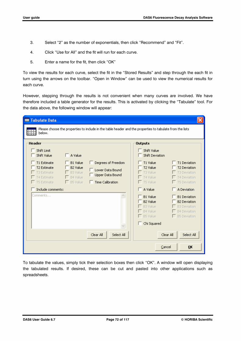
User guide DAS6 Fluorescence Decay Analysis Software
DAS6 User Guide 6.7 Page 72 of 117 © HORIBA Scientific
3. Select “2” as the number of exponentials, then click “Recommend” and “Fit”.
4. Click “Use for All” and the fit will run for each curve.
5. Enter a name for the fit, then click “OK”
To view the results for each curve, select the fit in the “Stored Results” and step through the each fit in
turn using the arrows on the toolbar. “Open in Window” can be used to view the numerical results for
each curve.
However, stepping through the results is not convenient when many curves are involved. We have
therefore included a table generator for the results. This is activated by clicking the “Tabulate” tool. For
the data above, the following window will appear:
To tabulate the values, simply tick their selection boxes then click “OK”. A window will open displaying
the tabulated results. If desired, these can be cut and pasted into other applications such as
spreadsheets.

User guide DAS6 Fluorescence Decay Analysis Software
DAS6 User Guide 6.7 Page 73 of 117 © HORIBA Scientific
9. Using Microscope Files
DAS has the ability to read and analyse microscope files produced by the HORIBA Scientific DynaMyc time-resolved fluorescence microscope and DataStation.
A single .das microscope file contains the following data:
A microscope image
A collection of X and Y pixel co-ordinates
A decay dataset for each pixel
A prompt (optional)
9.1 Analysing a Microscope File
Microscope files can be fitted in one of three ways depending on the fit chosen from the drop-down list at the bottom of the “Information Area” and then clicking the “Fit” button to the right of the list.
1. Batch Fit- This allows a fit calculation (up to 5 exponentials) to be performed sequentially on
many separate decay curves. Batch analysis is useful when you wish to fit several curves to the
same underlying exponential decay model but the curves are expected to have unrelated decay
lifetimes. For more information on this fit technique, see section 8 of this document.
2. Sum Fit- This method first sums all of the decay curves together and the resulting data set is then fitted to determine the lifetimes present. The lifetimes found are then globally applied to all the individual decays allowing the ‘B’ (amplitude) values to be calculated for each of the curves. This technique allows you to fit the data while using the fact that lifetimes present between decays are linked. To perform a Sum fit, depress the ‘Sum’ button on the toolbar then click the “Fit” button at the bottom of the “Information Area”
3. Global fit- This fit can only be applied on a file containing less than 100 decays. See section 7 of this manual for more information.
9.2 Viewing the Mapped Data
After a fit has been performed, the resulting fit parameters can be viewed graphically by overlaying them on top of the microscope image. If no fit has been performed yet, the intensity data can still be mapped

User guide DAS6 Fluorescence Decay Analysis Software
DAS6 User Guide 6.7 Page 74 of 117 © HORIBA Scientific
by selecting ‘working data’ in the tree. Displaying the intensity map can be useful to extract the decays with the highest intensities.
The mapping window is displayed by clicking the ‘Map’ button in the toolbar at the top of the screen, as shown below.
This displays a window containing the microscope image and a matrix of ‘pixels’ on top of this. An image of this is shown in below. Features that should be noted in the mapping window:-
The fit parameter that you wish to analyse should be selected using the drop down box at the top left of the Map window
The pixels superimposed on the image may vary in colour; this variation represents the relative magnitude of a particular fit parameter.
Hovering the cursor over a particular individual pixel allows you to view the value of its associated fit parameter at the top of the screen. Also, when clicking on a particular pixel, the fitted lifetime data of the selected pixel is displayed in the Main DAS window behind the Map window.
Graphs of a selected fit parameter are displayed at the bottom left of the Map window. By default, a graph of the distribution of the values of the parameter is shown. This distribution applies to the values found across all of the pixels plotted on the image.
Alternatively, by clicking a tab, the distribution graph can be replaced by a graph of the profile of a ‘slice’ across the image. This graph can display the fit parameter values as a function of either X or Y coordinates across the image.
Several options are available to customise the view. These options are described in the figure below.

User guide DAS6 Fluorescence Decay Analysis Software
DAS6 User Guide 6.7 Page 75 of 117 © HORIBA Scientific
9.3 Menu description
Map options:
Colour scale: displays the fit parameter map in false colours
Mouse cursor
coordinates
Distance between
adjacent pixels
Parameter to
be displayed
Transparency control
of the map over the
fluorescence image
(camera image)
Distribution of
selected parameter
over all the decays
Display of the fit parameters when hovering over a pixel
Mouse cursor
coordinates
Distance between
adjacent pixels
Parameter to
be displayed
Transparency control
of the map over the
fluorescence image
(camera image)
Distribution of
selected parameter
over all the decays
Display of the fit parameters when hovering over a pixel
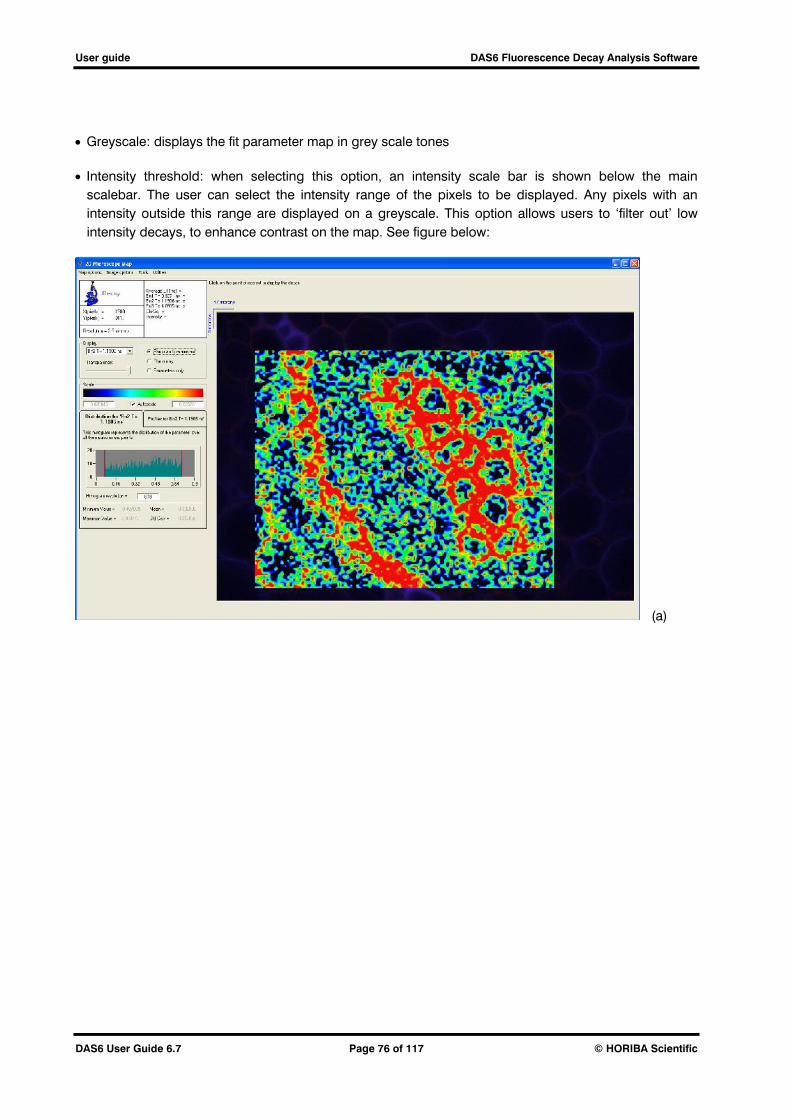
User guide DAS6 Fluorescence Decay Analysis Software
DAS6 User Guide 6.7 Page 76 of 117 © HORIBA Scientific
Greyscale: displays the fit parameter map in grey scale tones
Intensity threshold: when selecting this option, an intensity scale bar is shown below the main scalebar. The user can select the intensity range of the pixels to be displayed. Any pixels with an intensity outside this range are displayed on a greyscale. This option allows users to ‘filter out’ low intensity decays, to enhance contrast on the map. See figure below:
(a)
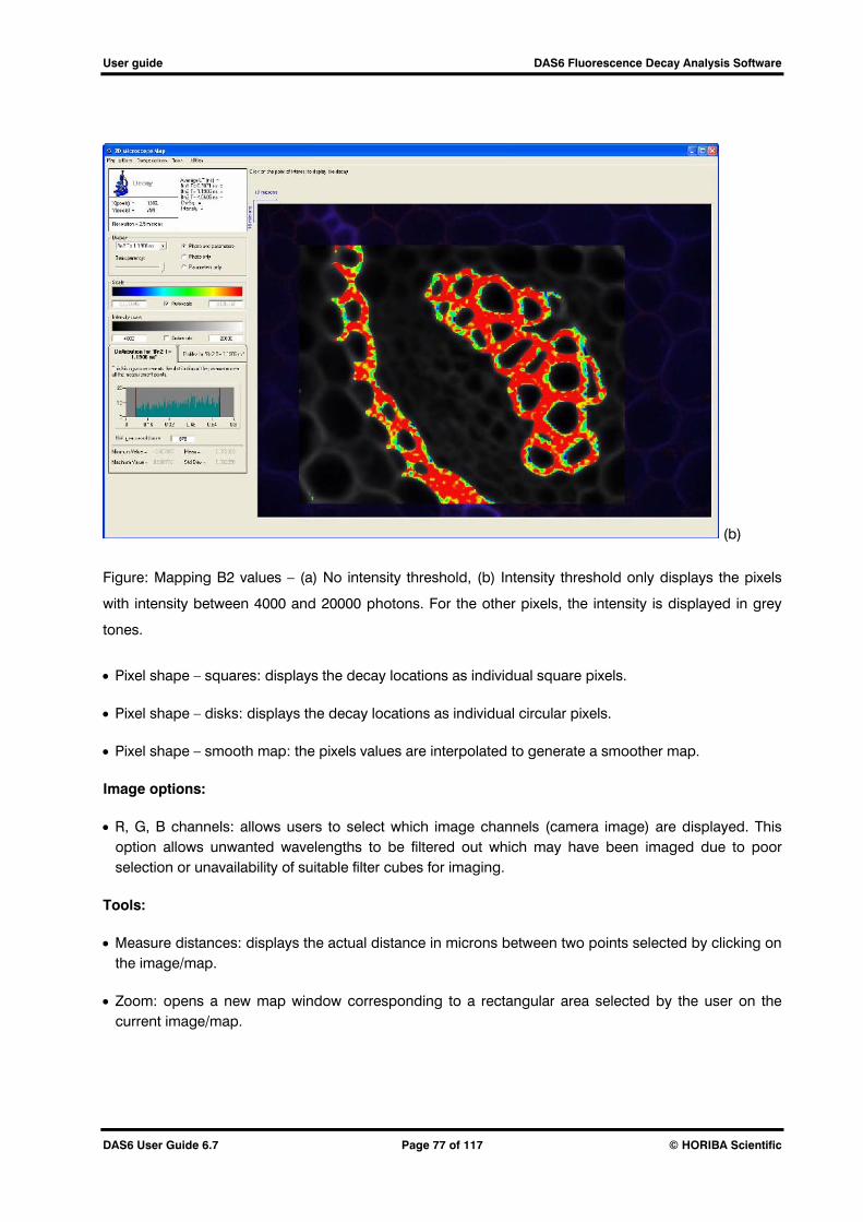
User guide DAS6 Fluorescence Decay Analysis Software
DAS6 User Guide 6.7 Page 77 of 117 © HORIBA Scientific
(b)
Figure: Mapping B2 values – (a) No intensity threshold, (b) Intensity threshold only displays the pixels
with intensity between 4000 and 20000 photons. For the other pixels, the intensity is displayed in grey
tones.
Pixel shape – squares: displays the decay locations as individual square pixels.
Pixel shape – disks: displays the decay locations as individual circular pixels.
Pixel shape – smooth map: the pixels values are interpolated to generate a smoother map.
Image options:
R, G, B channels: allows users to select which image channels (camera image) are displayed. This option allows unwanted wavelengths to be filtered out which may have been imaged due to poor selection or unavailability of suitable filter cubes for imaging.
Tools:
Measure distances: displays the actual distance in microns between two points selected by clicking on the image/map.
Zoom: opens a new map window corresponding to a rectangular area selected by the user on the current image/map.
User guide DAS6 Fluorescence Decay Analysis Software
DAS6 User Guide 6.7 Page 78 of 117 © HORIBA Scientific
FRET: this option allows the user to enter the lifetime of the FRET donor in absence of the FRET acceptor. It is then possible to display maps for the FRET efficiency and the FRET ratio R/Ro. These parameters are defined as:
FRET efficiency: E = 1 – (D-A / D) , where D-A is the donor fluorescence lifetime in presence of the acceptor and D is the donor fluorescence lifetime in the absence of the acceptor.
E = 1 / (1 + r/Ro)6 where r is the donor-to-acceptor separation distance and Ro is the Förster distance
of the donor-acceptor pair, i.e. the distance at which the energy transfer efficiency is 50%.
Utilities:
Print map: prints the current map display. The user can select to print the map, the statistical distribution and/or the detailed raw data of the map.
Save map: saves the map as an image file, in bmp, jpeg or gif format.
Export data: exports the map raw data as a text file.
User guide DAS6 Fluorescence Decay Analysis Software
DAS6 User Guide 6.7 Page 79 of 117 © HORIBA Scientific
10. Creating DAS Files
The DAS6 Decay Analysis Software uses a custom file type: “.das”. This data set (commonly called a
DAS file) allows you to store the results of your fits, alongside the data used to create them, and to
access all of the data at any time using HORIBA Scientific software.
There are a variety of ways to produce .das files that can be read by the DAS software. These include:
Using the DataStation software from HORIBA Scientific (HORIBA Jobin Yvon IBH)
Importing raw text or IBH binary files into the DAS software using the File -> New menu
command
Using the supplied DAS File Conversion Utility (DFCU) to read .das, IBH and raw text files
10.1 Types of DAS File
DAS files can be used to store 5 types of data. These types are listed in Table 1 along with the details of
their contents, possible fit types and how to create them.
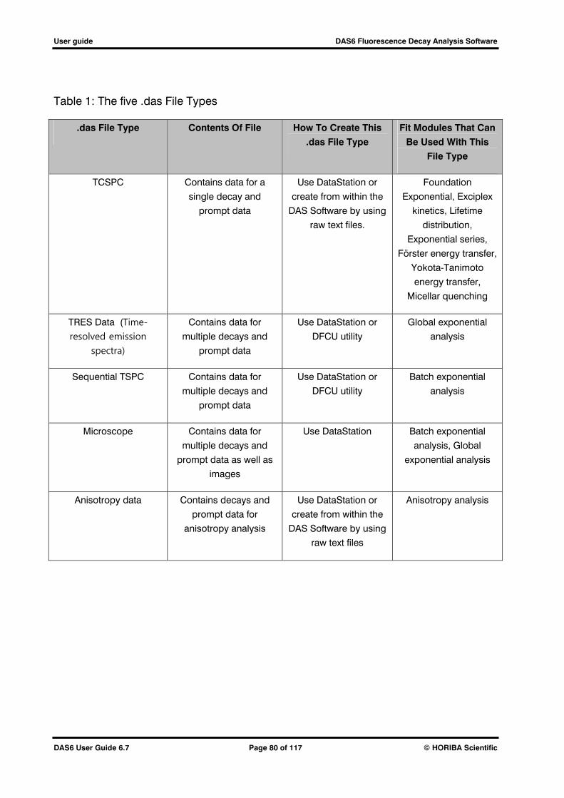
User guide DAS6 Fluorescence Decay Analysis Software
DAS6 User Guide 6.7 Page 80 of 117 © HORIBA Scientific
Table 1: The five .das File Types
.das File Type Contents Of File How To Create This
.das File Type
Fit Modules That Can
Be Used With This
File Type
TCSPC Contains data for a
single decay and
prompt data
Use DataStation or
create from within the
DAS Software by using
raw text files.
Foundation
Exponential, Exciplex
kinetics, Lifetime
distribution,
Exponential series,
Förster energy transfer,
Yokota-Tanimoto
energy transfer,
Micellar quenching
TRES Data (Time-
resolved emission
spectra)
Contains data for
multiple decays and
prompt data
Use DataStation or
DFCU utility
Global exponential
analysis
Sequential TSPC Contains data for
multiple decays and
prompt data
Use DataStation or
DFCU utility
Batch exponential
analysis
Microscope Contains data for
multiple decays and
prompt data as well as
images
Use DataStation Batch exponential
analysis, Global
exponential analysis
Anisotropy data Contains decays and
prompt data for
anisotropy analysis
Use DataStation or
create from within the
DAS Software by using
raw text files
Anisotropy analysis

User guide DAS6 Fluorescence Decay Analysis Software
DAS6 User Guide 6.7 Page 81 of 117 © HORIBA Scientific
10.2 Importing Data into DAS
There are a several ways to get data into the DAS software depending on which of the file types you wish
to create. The figure below illustrates the possible ways to import data:
DAS files are created by default when fluorescence lifetime measurements are made using the
Datastation software (method 2). For more information on using Datastation to produce DAS files, please
see the Datastation user manual. The remainder of this chapter deals with how to use methods 1 and 3
to import data into the DAS software.
Figure a: Methods of importing Data into DAS Software
Measured Decay
and Prompt Data
DATASTATION
SOFTWARE
DAS
SOFTWARE
.das files of type
TRES or Sequential DFCU
SOFTWARE
Decay and Prompt
Data from a raw
text file or any .das
/ IBH file
.das files of all types
Raw text files can be read
directly into the DAS software by
using the DAS menu ‘File->New’.
This data can be used to create
.das files of type TCSPC and
Anisotropy.
1
2
3

User guide DAS6 Fluorescence Decay Analysis Software
DAS6 User Guide 6.7 Page 82 of 117 © HORIBA Scientific
10.3 Creating a Decay Analysis Data Set Using DAS
The creation of a decay analysis data set is described below using the example files “DasPrompt.IBH”,
“DasDecay.IBH” and “DasFile.DAS”. These are respectively a prompt, decay and the resulting DAS file.
1. Start DAS and click on the “New” tool.
2. In the pop-up window select “TCSPC” and then click “New”.
3. Click “Browse” to open a file explorer window. Note that IBH is the default file type listed in
the “Files of Type” box. However, opening the drop down menu for this box you will see that
various other file types are supported (including simple text files).
4. Use the file explorer to find and select the file “DasPrompt.IBH”.
5. You have just selected the prompt file. In the pop-up window, click “Next” then repeat the
process to select file “DasDecay” to select the prompt.
6. Click “Next” and then, in the pop-up window enter a name for the DAS data set. In this
example type “DasFile”. The resultant .DAS file will be saved in a location that can be set by
the user in the Tools->Settings->Folder window. The default location is to save the newly
created file in the same folder as the imported decay data.
7. Click the “Finish” button to complete the process.
The screen will appear as shown below, and the new data set will be ready for use.

User guide DAS6 Fluorescence Decay Analysis Software
DAS6 User Guide 6.7 Page 83 of 117 © HORIBA Scientific
Note that, because one of the IBH files contains a time calibration, this information was transferred
automatically to the new DAS file. When importing some other types of files, an extra step to enter the
time calibration may be included. Alternatively the time calibration can be entered (or changed) from the
DAS6 “Edit/Time Calibration” menu selection.
Finally, selection of a prompt in steps 4 and 5 above is optional (select ‘skip’), but selection of the decay
is mandatory.

User guide DAS6 Fluorescence Decay Analysis Software
DAS6 User Guide 6.7 Page 84 of 117 © HORIBA Scientific
10.4 Creating an Anisotropy Data Set Using DAS
Creation of an anisotropy data set is very similar to the process described in section 10.1 for a decay analysis data set. However, in this case these can be between two and five files involved.
1. Start DAS and click on the “New” tool.
2. In the pop-up window select “Anisotropy” and then click “New”. A pop-up window will appear as
shown below.
3. Select decay files containing the crossed decay Yvh(i) and the parallel decay Yvv(i). Selection of
files for these is compulsory.
4. Click “Finish” if no other data needs to be entered, or “Next” to proceed to the next data input
screen,
5. Optionally, select a prompt file then click “Finish” or “Next”.
6. Optionally, select files for calculation the g-factor then click “Finish”.
When “Finish” is selected, enter a filename for the data set. The data set will then be ready for use.
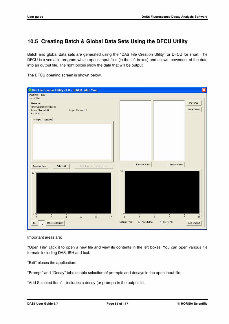
User guide DAS6 Fluorescence Decay Analysis Software
DAS6 User Guide 6.7 Page 85 of 117 © HORIBA Scientific
10.5 Creating Batch & Global Data Sets Using the DFCU Utility
Batch and global data sets are generated using the “DAS File Creation Utility” or DFCU for short. The DFCU is a versatile program which opens input files (in the left boxes) and allows movement of the data into an output file. The right boxes show the data that will be output.
The DFCU opening screen is shown below.
Important areas are:
“Open File” click it to open a new file and view its contents in the left boxes. You can open various file formats including DAS, IBH and text.
“Exit” closes the application.
“Prompt” and “Decay” tabs enable selection of prompts and decays in the open input file.
“Add Selected Item” – includes a decay (or prompt) in the output list.

User guide DAS6 Fluorescence Decay Analysis Software
DAS6 User Guide 6.7 Page 86 of 117 © HORIBA Scientific
“Output Type” – radio buttons which choose either batch or global format for the output file.
“Build Output” – button which starts the process of building the batch fit (sequential TCSPC) or global fit (TRES) output file. A filename should be input for the resulting DAS file.
The order of items in the output list can be adjusted with the Move Up/Down buttons, items can also be removed from the list.
10.6 Using Text Files with DAS6
DAS6 can import data from text files in addition to the older IBH v4.2 binary format prompt and decay
files. The text files must contain only the channel data (without channel numbers or any time information)
and be one data value per-line. All text data files are assumed to start from channel number 0. The first
two data points will be lost in the conversion, if these channels are important to the data then you should
pad the data with two leading zeros as the first two data lines in the file.
To import a text file you should create a new DAS file as normal but select “Text Files (*.txt)” from the file
open dialogue box. If the imported file does not conform to the above specification an error message will
be displayed. When loading decay data from a text file you will be prompted as to whether you want
Poissonian (for photon counting data) or Gaussian variances generated from the data. Appended
variance data is not supported.
The easiest way to get the data from other file types into DAS6 is to load your raw ASCII data into a
spreadsheet (e.g. Microsoft Excel) and then trim any excess text before saving the file. The saved file can
then be imported into DAS6.
10.7 Custom Filters
Custom file loading filters can be incorporated into the DAS6 software for ease of use. Please contact
HORIBA Scientific IBH if you are interested in using this service.
The current release imports:
IBH v4.2 files (from the older IBH MS-DOS software)
Text files (as described above)
Edinburgh Instruments Ltd. text files (*.DAT) that can be exported from EI software.
Globals Unlimited files. These contain both prompt and decay information and should be
imported as prompt files.
Ortec Maestro Integer CHN files.

User guide DAS6 Fluorescence Decay Analysis Software
DAS6 User Guide 6.7 Page 87 of 117 © HORIBA Scientific
11. When a Prompt cannot be measured
There are situations when it is not physically possible to measure a prompt. Two examples of this are:
When UV illumination (e.g. from a 260nm nanoled) is used to excite a sample but the detection
photomultiplier tube has a glass window and therefore has no sensitivity at the excitation
wavelength.
When visible illumination is used to excite a dye which fluoresces in the NIR and the detection
photomultiplier tube has no sensitivity in the visible (e.g. Hamamatsu H10330 which has a cut-off
at 950nm).
Two options are available to provide an estimated ‘prompt’. One option is to take a measurement using
a dye with a very short wavelength and use this as a prompt. The other procedure is to measure the
fluorescence from a dye with a known lifetime and then recover the prompt using a fast Fourier transform
(FFT).
An example dataset is shown below.
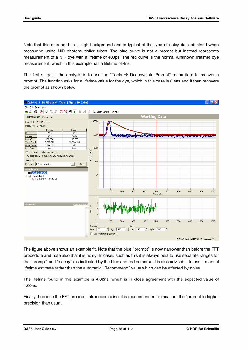
User guide DAS6 Fluorescence Decay Analysis Software
DAS6 User Guide 6.7 Page 88 of 117 © HORIBA Scientific
Note that this data set has a high background and is typical of the type of noisy data obtained when
measuring using NIR photomultiplier tubes. The blue curve is not a prompt but instead represents
measurement of a NIR dye with a lifetime of 400ps. The red curve is the normal (unknown lifetime) dye
measurement, which in this example has a lifetime of 4ns.
The first stage in the analysis is to use the “Tools Deconvolute Prompt” menu item to recover a
prompt. The function asks for a lifetime value for the dye, which in this case is 0.4ns and it then recovers
the prompt as shown below.
The figure above shows an example fit. Note that the blue “prompt” is now narrower than before the FFT
procedure and note also that it is noisy. In cases such as this it is always best to use separate ranges for
the “prompt” and “decay” (as indicated by the blue and red cursors). It is also advisable to use a manual
lifetime estimate rather than the automatic “Recommend” value which can be affected by noise.
The lifetime found in this example is 4.02ns, which is in close agreement with the expected value of
4.00ns.
Finally, because the FFT process, introduces noise, it is recommended to measure the “prompt to higher
precision than usual.
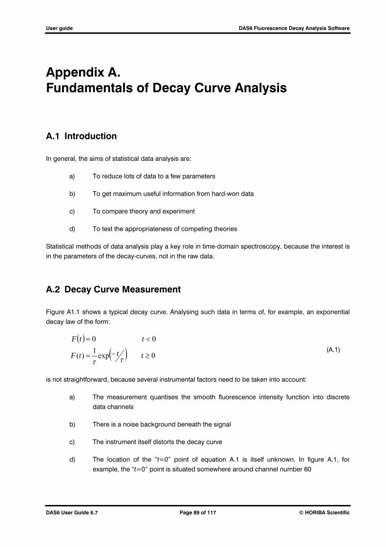
User guide DAS6 Fluorescence Decay Analysis Software
DAS6 User Guide 6.7 Page 89 of 117 © HORIBA Scientific
Appendix A. Fundamentals of Decay Curve Analysis
A.1 Introduction
In general, the aims of statistical data analysis are:
a) To reduce lots of data to a few parameters
b) To get maximum useful information from hard-won data
c) To compare theory and experiment
d) To test the appropriateness of competing theories
Statistical methods of data analysis play a key role in time-domain spectroscopy, because the interest is
in the parameters of the decay-curves, not in the raw data.
A.2 Decay Curve Measurement
Figure A1.1 shows a typical decay curve. Analysing such data in terms of, for example, an exponential
decay law of the form:
0exp1
)(
00
tttF
ttF
(A.1)
is not straightforward, because several instrumental factors need to be taken into account:
a) The measurement quantises the smooth fluorescence intensity function into discrete
data channels
b) There is a noise background beneath the signal
c) The instrument itself distorts the decay curve
d) The location of the “t=0” point of equation A.1 is itself unknown. In figure A.1, for
example, the “t=0” point is situated somewhere around channel number 60
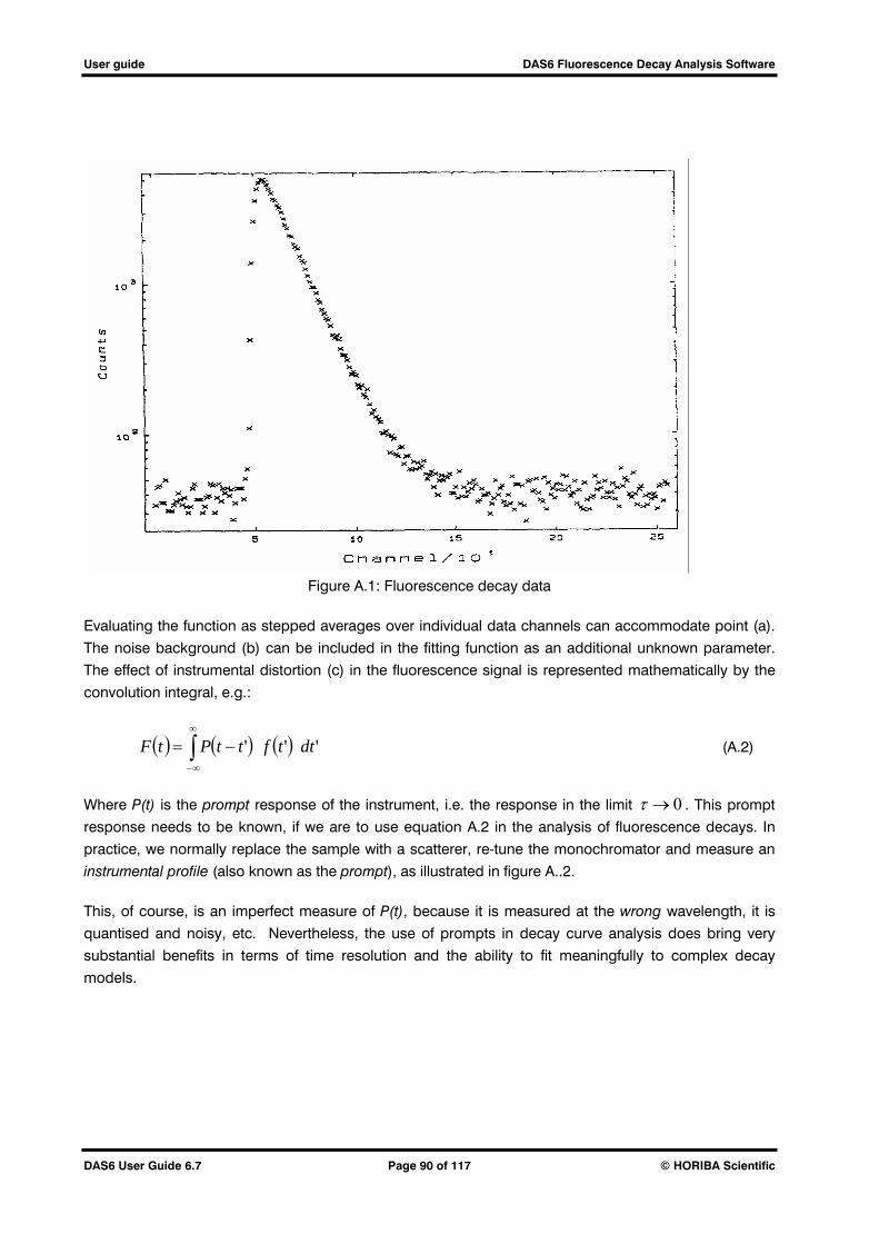
User guide DAS6 Fluorescence Decay Analysis Software
DAS6 User Guide 6.7 Page 90 of 117 © HORIBA Scientific
Figure A.1: Fluorescence decay data
Evaluating the function as stepped averages over individual data channels can accommodate point (a).
The noise background (b) can be included in the fitting function as an additional unknown parameter.
The effect of instrumental distortion (c) in the fluorescence signal is represented mathematically by the
convolution integral, e.g.:
''' dttfttPtF (A.2)
Where P(t) is the prompt response of the instrument, i.e. the response in the limit 0 . This prompt
response needs to be known, if we are to use equation A.2 in the analysis of fluorescence decays. In
practice, we normally replace the sample with a scatterer, re-tune the monochromator and measure an
instrumental profile (also known as the prompt), as illustrated in figure A..2.
This, of course, is an imperfect measure of P(t), because it is measured at the wrong wavelength, it is
quantised and noisy, etc. Nevertheless, the use of prompts in decay curve analysis does bring very
substantial benefits in terms of time resolution and the ability to fit meaningfully to complex decay
models.
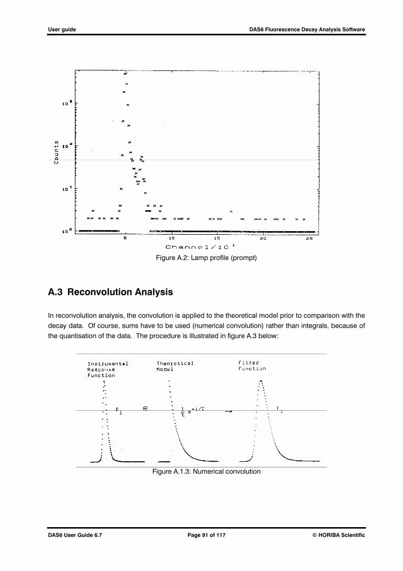
User guide DAS6 Fluorescence Decay Analysis Software
DAS6 User Guide 6.7 Page 91 of 117 © HORIBA Scientific
Figure A.2: Lamp profile (prompt)
A.3 Reconvolution Analysis
In reconvolution analysis, the convolution is applied to the theoretical model prior to comparison with the
decay data. Of course, sums have to be used (numerical convolution) rather than integrals, because of
the quantisation of the data. The procedure is illustrated in figure A.3 below:
Figure A.1.3: Numerical convolution
User guide DAS6 Fluorescence Decay Analysis Software
DAS6 User Guide 6.7 Page 92 of 117 © HORIBA Scientific
Why this way? Why reconvolute rather than deconvolute? If one could deconvolute the data, then
comparison with the kinetic model would be very direct. The answer is stability. Deconvolution of
experimental data is an ill-posed problem, because the effect of convolution is a smearing out, and
therefore a loss of information. You cannot regain the lost information by reversing the action. What you
can do is to apply a similar smearing action to the kinetic model, prior to comparison with the
experimental data. This is reconvolution.
A.4 Shift
The calculation of the fitted function, as in figure A.3 also determines the position among the data
channels of time t=0 (section A.2, point (d)), since this is directly related to the position of the prompt
P(i). However, a small mis-match in positioning is inevitable, because of quantisation, noise and
wavelength effects, etc., inherent in the less than perfect representation of the instrumental response by
the prompt. Since model functions, such as equation A.1, have their most rapid change at t=0, a small
positioning error can have a significant effect on the fit.
A.5 The Fitted Function
Finally, what started out as a simple exponential decay, now has the form:
iiPiF exp
1 (A.3)
from the numerical convolution (represented by ), and
iFBAiFD . (A.4)
for fitting the data. The integer “I” is used to denote the data channels. The shift parameter is
symbolic in this notation since you cannot have non-integral data channels. In practice a spill-over
algorithm is used for shifting. The parameter “A” is the noise background and “B” is an amplitude scaling
factor.
A.6 The Method of Least Squares
Equation A.4 now needs to be fitted to the fluorescence decay data Y(i) of figure A.1. The method used is
the method of least squares, which uses a quantity χ2 as a measure of mis-match between data and fitted
function. A discussion of the method of least squares can be found in almost any textbook on statistics.
In our example:

User guide DAS6 Fluorescence Decay Analysis Software
DAS6 User Guide 6.7 Page 93 of 117 © HORIBA Scientific
,,,22 BA (A.5)
The method strives to determine the best fit parameters ',',',' BA , that will yield the lowest possible
value of χ2.
A.7 The Meaning of χ2
By definition,
2
2
N
D
i
iFiY
(A.6)
deviation) standard its (i.e. , valuedatum theofy uncertaint lstatistica
A.1)equation (e.g.function fitting
A.1) figure (e.g. datadecay cefluorescen
iYi
iF
iY
D
The sum includes the N data channels selected for analysis. For any given value of i, the numerator
represents the actual deviation between the datum value Y(i) and the corresponding fitting function value
FD(i). The denominator represents the deviation expected from statistical (noise) consideration. Equation
A.6 can therefore be written as:
2
2
deviation expected
deviation actual
N
(A.7)
Now, if the fitting function is appropriate, then the minimum should be characterised by equality between
actual and expected deviations. The ratio (equation A.7) is then, on average, unity for each term of the
sum and:
N2 (A.8)
This is not quite right for two reasons:
a) The expected deviation is a statistical expectation, and therefore the mean value of a statistical distribution. This necessarily makes χ2 a statistical quantity with an associated distribution function.
b) The number of fitted parameters, n, needs to be taken into account. The quantity ν=(N-n) is called the number of degrees of freedom, and should be used in place of N.
A more accurate, though less precise statement of equation A.8 therefore is:
χ2 ≈ ν for a good fit

User guide DAS6 Fluorescence Decay Analysis Software
DAS6 User Guide 6.7 Page 94 of 117 © HORIBA Scientific
It is customary and convenient to normaliseχ2, so that its value is independent of ν:
χ2ν = χ2 / ν ≈ 1 for a good fit (A.9)
In photon counting experiments, the expected deviation, σ(i), can be estimated from the data, using the
Poissonian distribution. Thus:
2
1
iYi (A.10)
A.8 Local and Global χ2
In equation A.6, χ2 was defined as a sum over the individual data points of a fluorescence decay. It is
straightforward to extend this definition to include several such local sums, χ2 L1, χ2 L2 in a global χ2 G:
...22
122 LLG (A.11)
Global, rather than individual χ2-minimisation makes sense for families of decay curves with family
characteristics. Monomer/excimer decays, for example, should show amplitude changes but not decay
time changes with emission wavelength. You can therefore fit a whole family of excimer decay curves at
different wavelengths using the same decay times for all of them, but allowing for individual amplitudes.
Constraining the decay times in this way can often make a difference between curve representation and
kinetic sense!
The “Global Analysis Module” the HORIBA Scientific IBH library can work with a family of up to 100
decay curves, each with a corresponding instrument response function. Up to five family decay times
can be fitted, with individual amplitudes and noise backgrounds.
A.9 The Fitting Procedure
This consists of finding those values of the parameters (e.g. equation A.5) that will yield the lowest
possible value of χ2. In practice the procedures look for a χ2-minimum, which is not necessarily the same
thing.
Two basic procedures exist: liner and non-linear analysis. Linear analysis is restricted to linear
coefficients of the fitting function (e.g.A, B of equation A.5). Non-linear analysis works with any kind of
parameter. Since the Jobin Yvon IBH programs use both methods, it is instructive to go through both,
again using the single exponential function as an example.
Linear Analysis
From equations A.4 and A.6:

User guide DAS6 Fluorescence Decay Analysis Software
DAS6 User Guide 6.7 Page 95 of 117 © HORIBA Scientific
22 N
iFBAiYiw (A.12)
where 2 iiw is the data weight.
Since a minimum is characterised by a zero value for the gradient, we can find the best fit values A’ and
B’ by differentiation of equation A.12:
iFBAiYiw
A N
22
(A.13)
and
iFBAiYiFiw
B N
22
(A.14)
These gradients are zero for A=A’ and B=B’. Equations A.13 and A.14 can therefore be reduced to the
matrix equation:
iFiYiw
iYiw
B
A
iFiwiFiw
iFiwiw
'
'2 (A.15)
All the sums can be evaluated for given values of τ and ∆, thus A’ and B’ can be found by matrix
inversion.
Non-Linear Analysis
This is a polite phrase for brute force. You simply plug numbers into equation A.12 until you find the χ2-
minimum. The search strategy is a compromise between speed and stability. In simple cases, when the
parameters are independent of each other and the χ2 hypersurface is smooth, then stability is no
problem and a search algorithm can be optimised for speed. In the real world, however, parameters may
correlate and may need constraining. χ2 hypersurfaces may be unsymmetrical, bounded by asymptotic
flanks, structured and rough! No sensible search algorithm can cope with all situations.
In the HORIBA Scientific IBH algorithm, each parameter is iterated in a hierarchy, such that χ2 is
evaluated for several values of each parameter, as shown for τ in figure A.4 (circles). Once the minimum
has been traversed, the last three points are used in a parabolic interpolation to find the best value for
the parameter. χ2 is re-evaluated at this point (square). The statistical uncertainty of the parameter is then
determined from the width of the χ2 parabola. This search strategy is very stable, because only one
parameter is altered at any one time, and because care is taken to limit the step length. Careful fine-
tuning of the code has resulted in fast execution times – a factor that can become important when fitting
complex decay models.

User guide DAS6 Fluorescence Decay Analysis Software
DAS6 User Guide 6.7 Page 96 of 117 © HORIBA Scientific
Figure A.4 Non-linear minimisation
The linear parameters are evaluated afresh at each step of the non-linear search, thus ensuring that the
χ2 minimum, when reached, is a true minimum with respect to all the parameters of the fitted function.
Since the matrix inversion for the linear parameters is quick, this does not unduly slow down the fitting
procedure. Indeed, many fitting programs based on the Marquardt algorithm make no distinction
between linear and non-linear parameters. Such programs can therefore be slower to converge with
complex decay models, despite the intrinsic speed (and consequently poorer stability) of the algorithm
itself.
A.10 The Search Path
The HORIBA Scientific IBH algorithms search for the best parameters using the combined linear and
non-linear techniques described in section A.9. The search path for a single exponential component is
illustrated below:
In each line, a different value of T (= ) is tried. The XSQ (=χ2ν) value found for this value of T, with the
other parameters (A, B, SFT (=∆)) at their corresponding optimum values is given on the right. Each line
therefore summarises the results of a non-linear search for SFT, with matrix inversions for A and B at
each step. The first three lines of the printout define a minimum in XSQ vs T. The fourth line then gives
the parabolically interpolated best value of T.

User guide DAS6 Fluorescence Decay Analysis Software
DAS6 User Guide 6.7 Page 97 of 117 © HORIBA Scientific
In more complex cases, a similar hierarchy of iterative search loops is used. The sample printout below
is for a two-component exponential fit:
A.11 Weighted Residuals
A typical analysis, a double exponential fit, is shown in figure A.5. The same data analysed using a single
exponential model is shown in figure A.6. The crosses are fluorescence data Y(i). The line through them
is the best-fit function FD(i). The lower display box shows the weighted residuals, R(i), defined as:
deviation expected
deviation actual
i
iFiYiR D
(A.16)
comparison with equations A.6 and A.7 shows that:
22 N
iR (A.17)

User guide DAS6 Fluorescence Decay Analysis Software
DAS6 User Guide 6.7 Page 98 of 117 © HORIBA Scientific
Figure A.5: Analysis with two-exponential components

User guide DAS6 Fluorescence Decay Analysis Software
DAS6 User Guide 6.7 Page 99 of 117 © HORIBA Scientific
Figure A.6: Analysis with a single exponential component

User guide DAS6 Fluorescence Decay Analysis Software
DAS6 User Guide 6.7 Page 100 of 117 © HORIBA Scientific
The weighted residuals are an important means of assessing the goodness of fit because:
a) They show where misfits occur.
b) Their normalisation compensates for the varying data precision within the data set and
from data set to data set.
c) The deviations are expressed in a statistically meaningful way, in terms of the standard
deviations of the associated data noise.
d) The relationship between residuals and χ2, the fitting criterion, is straightforward.
These points are illustrated in figure A.6. This shows the same data as figure A.5, but analysed with a
single exponential model. The misfit is hardly apparent in the main display, but residuals of 18
standard deviations in the rising edge show clearly that a finite rise-time is present in the data.
A.12 Autocorrelation of Residuals
An alternative method of assessing the goodness of fit is to calculate the residuals autocorrelation
function, defined by:
T
t
dtttRt0'
''t'RT
Limit (A.18)
Of course, we know R(t) only in histogram form and only over the region of interest selected for fitting. In
practice the integral is replaced by a sum, and the range of decay times ∆t is limited to one half the
number of channels analysed, because of the necessarily finite range of integration. It is customary to
normalise A(∆t) so that A(0) = 1.
With randomly distributed residuals (a good fit) there should be no systematic correlation and the
autocorrelation function should be small and random for ∆t > 0. Systematic features in the residuals lead
to systematic structure in the autocorrelation function.
These points are illustrated in figure A.7 below. The two curves were calculated from the residuals of
figures A.5 and A.6. It is left as an exercise to the reader to identify the autocorrelation functions
corresponding to the one- and two-component fits.

User guide DAS6 Fluorescence Decay Analysis Software
DAS6 User Guide 6.7 Page 101 of 117 © HORIBA Scientific
Figure A.7: Autocorrelation of residuals
A.13 Non-Poissonian Data
Fluorescence decays can be measured by many different techniques. In particular, decay curves
measured using photomultiplier current sampling with a boxcar integrator or transient digitiser cannot
use the Poissonian data weighting scheme of equation A.10.
The DAS6 software was designed to analyse data from a variety of sources. Figure A.8 shows the rising
edge of the fluorescence signal from Cr3+ ions in a MgO matrix, showing that this state is populated by
energy transfer. The data were measured using a transient digitiser interfaced with a data averaging
computer. The statistical properties of this signal are more clearly Gaussian than Poissonian. This is
noted in the file header, by the signal averaging program. All subsequent analyses and manipulations of
these data by the DAS6 software then use and propagate these statistical properties in the appropriate
ways – again automatically and without user intervention. An appropriate message keeps the user
informed of what is being done.
In figure A.8 the value of XSQ and the normalisation of the residuals are calculated using Gaussian, not
Poissonian rules.

User guide DAS6 Fluorescence Decay Analysis Software
DAS6 User Guide 6.7 Page 102 of 117 © HORIBA Scientific
Figure A.8: Fluorescence decay measured with a transient digitiser (Data by courtesy of Dr. M. O’Neill, measured in the Photophysics Research Laboratory of Strathclyde University)

User guide DAS6 Fluorescence Decay Analysis Software
DAS6 User Guide 6.7 Page 103 of 117 © HORIBA Scientific
Appendix B. Analysis of Anisotropy Decays
B.1 Introduction
The anisotropy decay function, r(t) is defined by:
tI
tI
tItI
tItItr
s
d
vhvv
vhvv
2
(B.1)
“I” represents idealised (i.e. undistorted) fluorescence intensity. The subscripts “v” (vertical) and “h”
(horizontal) refer to the orientation of the polarisers (e.g. Ivh refers to a vertical excitation polariser and a
horizontal emission polariser). Similarly the subscripts “d” and “s” refer” to “sum” and “difference”
respectively. Ivv and Ivh need to be measured under identical conditions for equation B.1 to make sense.
In practice, a number of instrumental effects need to be taken into account when analysing anisotropy
data.
1. We observe Y(i), not I(t). Since reconvolution does not apply to the ratio function r(t), we have to
be more subtle in accounting for instrumental distortions.
2. If we combine Yvv(i) and Yvh(i) as in equation B.1, the resulting anisotropy decay curve is no
longer characterised by Poissonian statistics. Therefore, we have to be more subtle in
calculating data weights for analysing anisotropy decay curves.
3. Yvv(i) and Yvh(i) may or may not be measured under identical conditions. Indeed, considerable
care in the design of the apparatus and measurement technique is required to obtain truly
identical conditions.
B.2 Methods of Measuring Anisotropy Decays
The method(s) of analysis need to take into account the conditions under which Yvv(i) and Yvh(i) were
measured. The following conditions commonly apply:
1. Manual Measurement - it is often useful to be able to obtain some anisotropy decay information
without special apparatus. In such cases it is not possible to obtain identical conditions of
observation for parallel and crossed planes of polarisation. A vector reconvolution technique
(e.g. see section B.5) can be then used to extract anisotropy parameters in favourable cases.
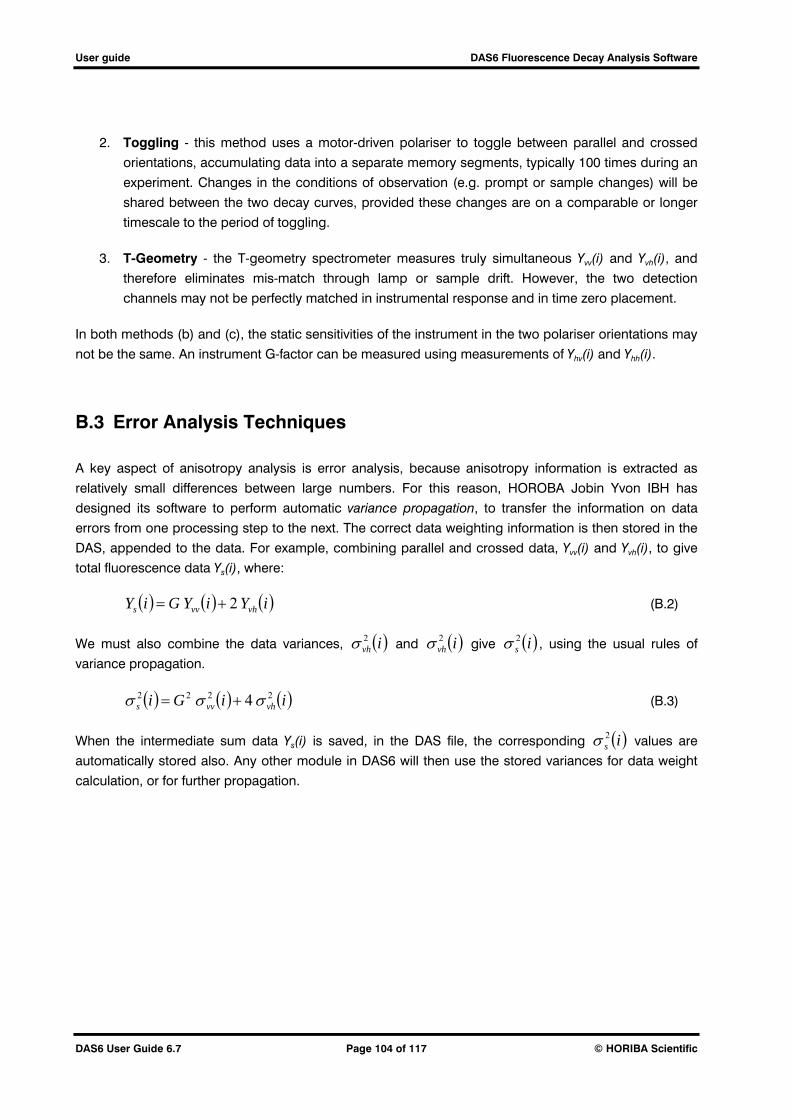
User guide DAS6 Fluorescence Decay Analysis Software
DAS6 User Guide 6.7 Page 104 of 117 © HORIBA Scientific
2. Toggling - this method uses a motor-driven polariser to toggle between parallel and crossed
orientations, accumulating data into a separate memory segments, typically 100 times during an
experiment. Changes in the conditions of observation (e.g. prompt or sample changes) will be
shared between the two decay curves, provided these changes are on a comparable or longer
timescale to the period of toggling.
3. T-Geometry - the T-geometry spectrometer measures truly simultaneous Yvv(i) and Yvh(i), and
therefore eliminates mis-match through lamp or sample drift. However, the two detection
channels may not be perfectly matched in instrumental response and in time zero placement.
In both methods (b) and (c), the static sensitivities of the instrument in the two polariser orientations may
not be the same. An instrument G-factor can be measured using measurements of Yhv(i) and Yhh(i).
B.3 Error Analysis Techniques
A key aspect of anisotropy analysis is error analysis, because anisotropy information is extracted as
relatively small differences between large numbers. For this reason, HOROBA Jobin Yvon IBH has
designed its software to perform automatic variance propagation, to transfer the information on data
errors from one processing step to the next. The correct data weighting information is then stored in the
DAS, appended to the data. For example, combining parallel and crossed data, Yvv(i) and Yvh(i), to give
total fluorescence data Ys(i), where:
iYiYGiY vhvvs 2 (B.2)
We must also combine the data variances, ivh2 and ivh
2 give is2 , using the usual rules of
variance propagation.
iiGi vhvvs2222 4 (B.3)
When the intermediate sum data Ys(i) is saved, in the DAS file, the corresponding is2 values are
automatically stored also. Any other module in DAS6 will then use the stored variances for data weight
calculation, or for further propagation.
User guide DAS6 Fluorescence Decay Analysis Software
DAS6 User Guide 6.7 Page 105 of 117 © HORIBA Scientific
B.4 Direct Analysis from Data
The first method makes use of the decay curves Yvv(i) and Yvh(i), together with the G-factor, to calculate
the anisotropy decay curve directly, point by point:
iY
iY
iYiYG
iYiYGiY
s
d
vhvv
vhvvr
2
(B.4)
The method can be used with data from toggling and T-geometry experiments. It does not use
reconvolution analysis and therefore does not require measurements of Pvv(i) or Pvh(i). The Yr(i) curve
obtained can then be analysed using the exponential fit module, in terms of a number of exponential
decay components, superimposed on a static anisotropy r (=A in the notation of the fit modules).
Figure B.2 shows an example of such an analysis. The method is very popular because it is quick, direct,
and gives an excellent visual inspection – important for judging whether interpretation is truly supported
by the measurement. The main disadvantage is that instrumental distortions remain unaccounted for –
you therefore cannot extract very short anisotropy decay times.

User guide DAS6 Fluorescence Decay Analysis Software
DAS6 User Guide 6.7 Page 106 of 117 © HORIBA Scientific
Figure B.2: Direct analysis of anisotropy decay data
Another point to note in figure B.2 is that the anisotropy data are reasonably well defined initially, but
become dramatically noisy as time proceeds. It is of the utmost importance to use correct data weights
in the analysis of such anisotropy data. If Poissonian rules were applied, the fit would be strongly
influenced by the noisy part of the data on the right, leading to spurious parameters, with residuals and
χ2 values that were wrongly scaled.
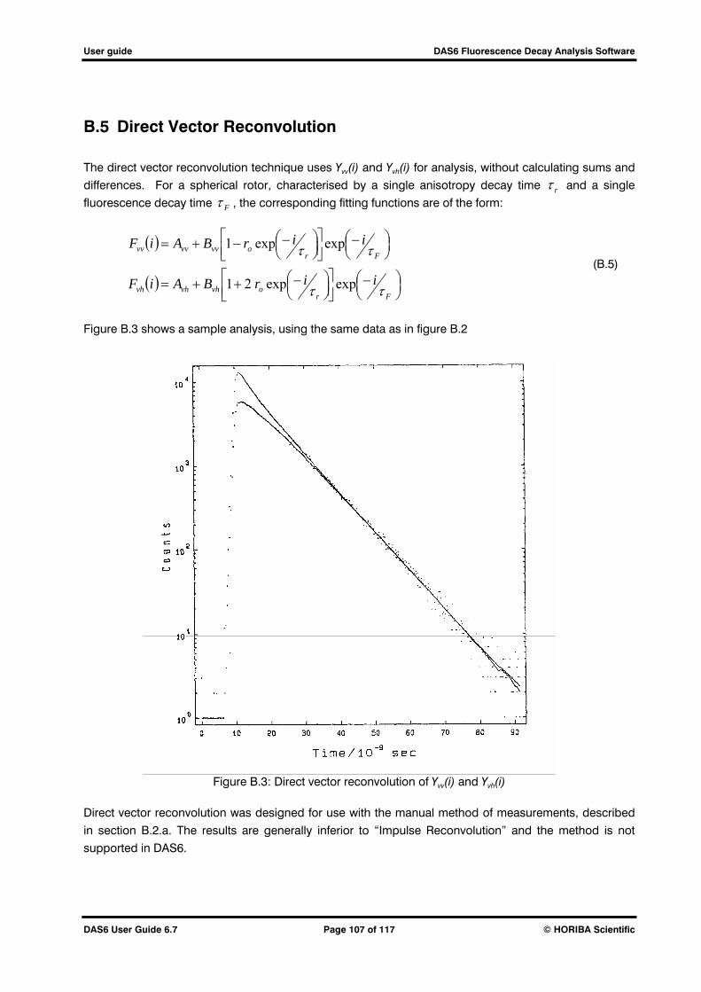
User guide DAS6 Fluorescence Decay Analysis Software
DAS6 User Guide 6.7 Page 107 of 117 © HORIBA Scientific
B.5 Direct Vector Reconvolution
The direct vector reconvolution technique uses Yvv(i) and Yvh(i) for analysis, without calculating sums and
differences. For a spherical rotor, characterised by a single anisotropy decay time r and a single
fluorescence decay time F , the corresponding fitting functions are of the form:
Frovhvhvh
Frovvvvvv
iirBAiF
iirBAiF
expexp21
expexp1
(B.5)
Figure B.3 shows a sample analysis, using the same data as in figure B.2
Figure B.3: Direct vector reconvolution of Yvv(i) and Yvh(i)
Direct vector reconvolution was designed for use with the manual method of measurements, described
in section B.2.a. The results are generally inferior to “Impulse Reconvolution” and the method is not
supported in DAS6.

User guide DAS6 Fluorescence Decay Analysis Software
DAS6 User Guide 6.7 Page 108 of 117 © HORIBA Scientific
B.6 Impulse Reconvolution
This method is considerably more powerful than the previous one, because the analysis is split into two
separate parts: analysis of Ys(i) followed by analysis of Yd(i).
The total fluorescence decay, Ys(i) is free of anisotropy effects and should be straightforward to analyse
separately, using 1-4 exponential components.
The difference decay, Yd(i) is considerably more complex, because it contains fluorescence as well as
anisotropy parameters. However, if we freeze the fluorescence parameters, the anisotropy parameters
should be much more readily obtainable. In impulse reconvolution this freezing is achieved by accepting
the results of the analysis of Ys(i) as a constraint. Without such a constraint, difference decay data
analysis would yield meaningless parameters.
Let Is(i), Id(i) and Ir(i) be impulse response functions (IRF) (i.e. decay curve shapes free of instrumental
distortion or artefact) for total, difference and anisotropy respectively. Then, from equation B.1:
iIiIiI drs . (B.6)
The point about writing equation B.1 in this way is that we can convolute both sides of equation B.6 with
P(i) and obtain two equivalent expressions for a fitting function for Yd(i). Is(i) is known, from the analysis
of Ys(i): this is the constraint in the analysis of Yd(i). Ir(i) is not known, but this is what we are after. The
impulse reconvolution module uses:
21inf
21inf
with
expexp21
BBrr
iBiBriI
o
rrr
(B.7)
Thus allowing two anisotropy decay times, together with or and r to be extracted from Yd(i).
The method is illustrated in figure B.4. Again, the same data as for figures B.2 and B.3 is used to
illustrate this technique. The total fluorescence decay was analysed with two exponential components,
using the exponential fitting modules. The impulse response function Is(i) calculated in this way then
formed the constraint in the impulse reconvolution, where the difference data were analysed in terms of
one anisotropy decay component, together with r .

User guide DAS6 Fluorescence Decay Analysis Software
DAS6 User Guide 6.7 Page 109 of 117 © HORIBA Scientific
Figure B.4: Impulse reconvolution analysis

User guide DAS6 Fluorescence Decay Analysis Software
DAS6 User Guide 6.7 Page 110 of 117 © HORIBA Scientific
B.7 Impulse Response Function Methods
Impulse response functions can be calculated for any fit, using the best-fit parameters. Unlike fitted
functions, impulse response functions (IRFs) represent the fitted model without instrumental distortion or
background noise. IRFs do not contain any data weights hence there is no basis for judging the
statistical validity of fits produced from them.
It can be see from figure B.2, that impulse response methods need more information to be measured
than the impulse reconvolution method. Because of this, impulse response function methods are not
supported in DAS6.

User guide DAS6 Fluorescence Decay Analysis Software
DAS6 User Guide 6.7 Page 111 of 117 © HORIBA Scientific
Appendix C. DAS6 Specifications
Operating systems supported: -
Microsoft Windows XP (32 bit)
Microsoft Windows Vista (32 bit)
Microsoft Windows 7 (32 / 64 bit)
Hardware requirements: -
1.5 GHz CPU Speed
1GB RAM
2GB hard disk space
Minimum screen resolution 1024 x 768
Over the page, Table 2 lists the specifications of the curve fitting features of DAS.
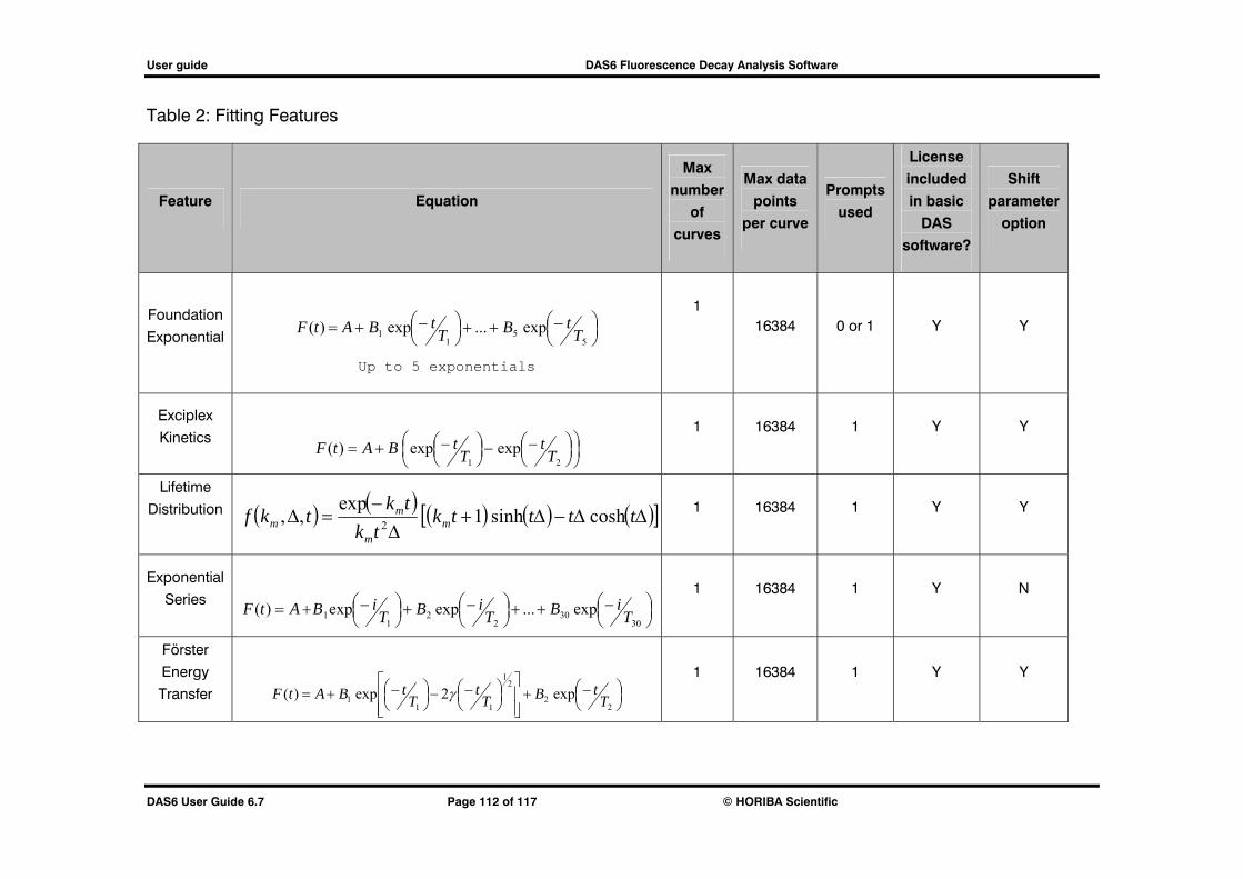
User guide DAS6 Fluorescence Decay Analysis Software
DAS6 User Guide 6.7 Page 112 of 117 © HORIBA Scientific
Table 2: Fitting Features
Feature Equation
Max
number
of
curves
Max data
points
per curve
Prompts
used
License
included
in basic
DAS
software?
Shift
parameter
option
Foundation
Exponential
55
11 exp...exp)( T
tBTtBAtF
Up to 5 exponentials
1
16384 0 or 1 Y Y
Exciplex
Kinetics
21expexp)( T
tT
tBAtF 1 16384 1 Y Y
Lifetime
Distribution
1 16384 1 Y Y
Exponential
Series
3030
22
11 exp...expexp)( T
iBTiBT
iBAtF 1 16384 1 Y N
Förster
Energy
Transfer
22
21
111 exp2exp)( T
tBTt
TtBAtF
1 16384 1 Y Y
ttttk
tk
tktkf m
m
mm coshsinh1
exp,,
2
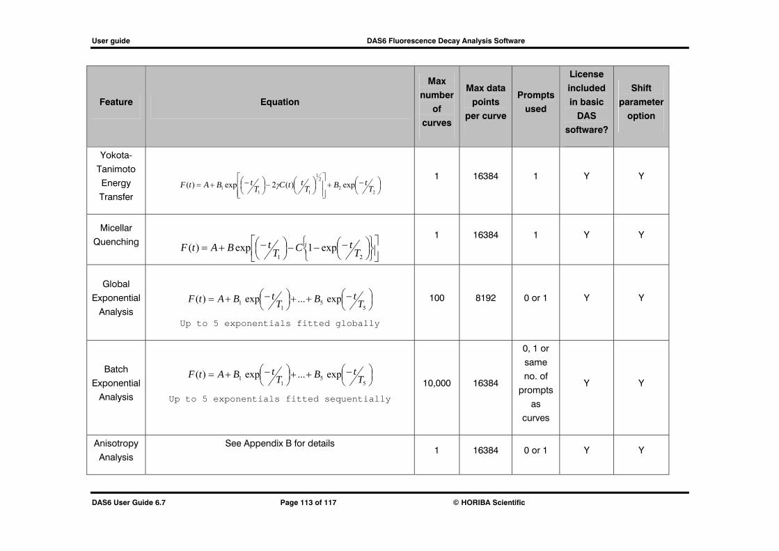
User guide DAS6 Fluorescence Decay Analysis Software
DAS6 User Guide 6.7 Page 113 of 117 © HORIBA Scientific
Feature Equation
Max
number
of
curves
Max data
points
per curve
Prompts
used
License
included
in basic
DAS
software?
Shift
parameter
option
Yokota-
Tanimoto
Energy
Transfer
22
21
111 exp)(2exp)( T
tBTttCT
tBAtF 1 16384 1 Y Y
Micellar
Quenching
21exp1exp)( T
tCTtBAtF
1 16384 1 Y Y
Global
Exponential
Analysis
55
11 exp...exp)( T
tBTtBAtF
Up to 5 exponentials fitted globally
100 8192 0 or 1 Y Y
Batch
Exponential
Analysis
55
11 exp...exp)( T
tBTtBAtF
Up to 5 exponentials fitted sequentially
10,000 16384
0, 1 or
same
no. of
prompts
as
curves
Y Y
Anisotropy
Analysis
See Appendix B for details 1 16384 0 or 1 Y Y

User guide DAS6 Fluorescence Decay Analysis Software
DAS6 User Guide 6.7 Page 114 of 117 © HORIBA Scientific
Feature Equation
Max
number
of
curves
Max data
points
per curve
Prompts
used
License
included
in basic
DAS
software?
Shift
parameter
option
Non-
Extensive
Distribution
5
1
11
/11)(k
qkkk
kttqBAtF 1 16384 0 or 1 N Y

User guide DAS6 Fluorescence Decay Analysis Software
DAS6 User Guide 6.7 Page 115 of 117 © HORIBA Scientific
Appendix D. How to access the DAS log files.
DAS creates a log file each time it runs to record in detail what happens during the session. If anything goes wrong with the application then the log file(s) must be send to HORIBA Scientific support staff so that they can trace the problem. Problems cannot be investigated unless a log file is provided.
The most recent log file is always named DAS6.log. The log files are always created in the application folder, this folder is chosen on installation with the default being:
C:\Program Files\HORIBA Scientific\DAS6\
If during a session of an application, a problem occurs and the application crashes then, when the application is next started, the previous incomplete log file will be identified and saved. This involves changing the name of the log file from DAS6.log to:
DAS6_yymmddhhmmss.LOG where yymmddhhmmss is the current date and time,
e.g. DAS_041225161510.log


[Design Concept]
The HORIBA Group application images are collaged in the overall design.Beginning from a nano size element, the scale of the story develops all the way to the Earth with a gentle flow of the water.
3880 Park Avenue, Edison, New Jersey 08820-3012, USA