5-1 Volume and shear viscosities, heat capacity and glass transition.

Today we're going to delve a little bit into the details of the relaxation process. And we're going to discover the main attributes of relaxation in silicate melts, one of those, which we'll see very quickly at the outset, is the so called equivalence, which means that no matter how the relaxation time of the system is determined, which properties we use or which experimental apparatus, if we're careful and we compare the results, in terms of the timescales of the experiment, then we discover that we get the same value, regardless of property investigated.

Very important at the outset for amorphous materials is to point out that when we're dealing with stress-strain relationships in such systems, free elasticity or for viscosity, that we should be careful to observe that there are two tensorial components of the deformation of the system.

There is a volume component, which essentially relates to changes in density, as a [reaction] reaction to changes in the volumetric stress, or the pressure.

And there is a shear component which reacts to changes in the shear stress in the system.

Now, luckily, numerically, for purposes of evaluating the relaxation time, we will discover in a moment that these have the same value.

In other words, the viscosity and the elasticity, either in a shear or a volume sense, are very, very similar in magnitude, which means that it makes it relatively easy to compare the relaxation times, regardless of these two tensorial components.

We can define a longitudinal value of either the elasticity or of the viscosity simply by adding the volume component to the shear component times four thirds.

If we do a test of the relative values of the volume and the shear viscosity, the viscous response to changes in pressure, for the volume, then the changes in shear stress, for the shear viscosity.

Then, we can see very quickly by comparing the longitudinal value of the viscosity, which is measure using longitudinal wave propagation, the damping of longitudinal waves and silicate liquids on the vertical axis here, and the shear viscosity along the horizontal axis, which is determined by common techniques for determining shear viscosity in the laboratory involving very large strains, that the one to one relationship that we would expect, in other words volume viscosity equal to shear viscosity, would obtain such that seven thirds of the longitudinal viscosity is equal to the shear viscosity, such that seven thirds of the shear viscosity is equal to the longitudinal viscosity.

And what you see here isn't a comparison of the experimental sets of data from the longitudinal and the shear viscosity and you see that they cluster around the one to one line.

So shear viscosity is approximately equal to volume viscosity.

And we can go forward now without being overly concerned about the relative contributions of shear and volume in our stress-strain relationships.

On the next graph, you see a plot of the two main thermal analysis determinations that are made on silicate liquids plotted one over the other.

On the top half of the diagram, you see a plot of the heat capacity versus the temperature on the horizontal axis.

And below it, you see a plot of the thermal expansivity of the liquid versus the same temperature scale.

And you will probably note immediately that there is a difference between these two curves.

We see, for example, in the case of the heat capacity curve on the left-hand side below the peak, below the glass transition, that there is a slight increase in the value of the heat capacity in the glassy state, whereas in the case of thermal expansion, we see no significant increase on the left hand side on the bottom.

You will also see that on the far right the curves behave differently.

You see that the heat capacity curve appears to be coming to an equilibrium value, on the right hand side, beyond the peak, where it hits the metastable equilibrium liquid state, whereas the more ragged, more noisy thermal expansion curve appears to fall and fall and fall and not reach equilibrium.

This particular attribute above the glass transition temperature is an experimental artifact of the way that thermal expansion is measured in these systems.

These are free standing cylinders, which, as they reach the glass transition and begin to have the ability to flow viscously and to relax, are no longer capable of yielding their absolute value of thermal expansion using this technique.

And, therefore, at the extreme far right of the expansivity curve, the results are falsified by this artifact.

Doesn't need to concern us at the moment, as you might have suspected.

And what we see in the middle is the most important point.

We see the peak value of the thermal expansion on the bottom and the peak value of the Cp, the heat capacity on the top, at precisely as accurately as we can measure it at exactly the same value of temperature.

And this is the first demonstration that I give you of the so-called equivalence of this glass transition.

These are two completely different experiments.

In the case of the heat capacity experiments, when measuring heat fluxes, as we heat up a sample and see how much it's going to cost us, in terms of the heat which goes in.

And then, the second case, we're measuring length of a standing cylinder, in this case, of a glass initially, which is being heated up and crossed the glass transition, and we're measuring the height of the cylinder in a sub-micron accuracy with a variable displacement transducer.

So these three experiments would normally be found in very different labs in any institution, and yet they give us the same number, the same result, the same peak value.

And, therefore, they both identify a lot is appearing to be a unique value of that temperature.

Now, very important is in order for these two curves to be comparable, in order for us to observe that peak occurring at the same position on both cases, we must have had identical materials, of course, in both experiments that doesn't only involve their chemistry, it also involves their thermal history.

In other words, the glass which we use at room temperature to initiate the thermal run in both of these cases, is the same chemistry, the same mix if you will, the same melt.

And it has been also prepared in the same manner by cooling it to the glassy state.

And then, when we reheat this, a structurally identical material in both of these experiments, we're allowed to observe the fact that the glass transition peak expresses itself similarly in both cases.

We'll see many more examples of equivalence.

But this first one can be brought home by normalizing the comparison of those two curves that you've seen.

What you see here now is the same data, but it is plotted now as a normalized plot.

And you can see on the vertical axis, dimensionless units going from zero at the bottom, to a peak height, equal to 1.0 at the top.

And if I normalize both of them, what have I done?

I've taken the glassy value of the relative property of the derivative property, be it the heat capacity or be in the thermal expansivity, and I've clearly set that equal to zero.

That's why you see these two lines now not deviating from a value of zero until I begin to deviate from the glassy state.

And as I go to the peak, you see I've set, arbitrarily, the peak value of both of those curves to be equal to one and, therefore, they meet again at 1.0.

Most importantly, is they meet at the same temperature, and secondly, if you follow the trace of the curve, as you rise up from the glassy state to the peak value at the glass transition, you see that the two curves overlap and overlay each other quite well.

So it's showing that, actually, the path, in terms of the change in property in driving from a glassy to a liquid state, is also the same if I have the same chemistry.

And if I have the same thermal history of the material that I'm working with.

You do see that on the right hand side in the liquid state the two curves deviate from one another.

No question.

The curves are not similar when we reach the right hand side.

The reason we just mentioned, it is an experimental artifact in this case because the extreme right of the noisier curve here, which is the dV⁄dT curve, is flawed because the cylinders are beginning to viscously collapse.

And thermal expansion can't be measured using that technique so easily.

So it's an experimental detail.

And no, and in no way, impacts on the equivalence statement that we've made.

5-2 Glass transition, hydrous granitic systems.

Now look at this next plot.

It seems rather benign.

It's a plot of the glass transition temperature.

In this case, the glass transition temperature has been defined how?

It's been defined implicitly as a time scale.

Remember that I told you that we have a time-temperature relationship, which we call

the glass transition.

And in order to talk about a glass transition temperature, either everyone in the room

has to agree on a certain convention, implicitly, or it has to be stated explicitly.

The latter is perhaps better.

And so, what you see on the vertical axis here is an explicit statement about what glass

transition temperature am I speaking of.

I'm speaking of the one, which corresponds to a particular relaxation time, which, in

turn, corresponds to a particular shear viscosity, through the Maxwell relation as we've

seen previously.

And the shear viscosity that we've chosen is stated here very precisely at 10 to the 12.38

Pascal seconds.

Now if you look on the horizontal axis you see water content.

Now this is one of the first mentions that we make of significant water.

Water is the most common volatile substance in these melts.

We've mentioned that at the beginning of the course, and you can see here that the water

contents we're talking about are very, very substantial.

These are weight percents of water and they run up to many, many weight percent.

So it means that it is relevant in volcanic systems to concern ourselves with water

contents in silicate liquids, which run up to 3, 4, 5, 6 weight percent of water.

And, as we'll see later, the details of how these things oversaturate, when they're rising

to the surface before an eruption, is a large, large control on how volcanic eruptions

actually take place.

And one of the reasons that it's so sensitive that eruptive behavior really is sensitively

dependent on water content, is in essence given by this plot.

You see the glass transition temperature has a function of dissolved water content in the

melt.

And what you see is a very, very large vertical scale in temperature.

You see it running, in this case, it's temperature in degrees Kelvin over approximately

400 degrees, 400 degrees Kelvin or 400 degrees Celsius.

Now, that implies that we have started from a very very dry melt at the beginning at

zero weight percent of water.

In nature, nothing is completely dry, but nevertheless in a laboratory it's relatively easy

for us to bring the water contents down to a few ppm, which we can describe

approximately as dry.

And you can see the data points, which run from that dry value at the extreme upper left

of the diagram, where we're up near 1100 Kelvin, at the glass transition temperature.

That's a very high glass transition temperature.

And then, it runs down, it runs down fairly fast, fairly steeply, as we add the first couple

8% of water to the system.

And then, it begins to flatten out, such that, if I go beyond 5 weight percent of water in

this diagram, I will more or less have a very, very subtle drop in the further variation of

Tg.

Now, all of the data points that have been taken to produce this curve have come from

very different experiments.

And that's why I show it to you at this point in time.

This is a triumph, if you will, of the equivalence principle.

Because there are four different techniques from five different studies, which have been

plotted on this curve.

And as you see very clearly, they all lie fairly tightly on this curve.

There have been volumetric measurements of the relaxation of this system.

There have been measurements of the viscosity of this system, through the Maxwell

relationship to determine the relaxation time.

There have been measurements of the heat capacity to determine the peaks on the heat

capacity curve and, and we'll see more if it in a moment, there have actually been

measurements of the structural role of water through spectroscopy in these liquids,

which also can be used to give a reaction time or a relaxation time of spectroscopic

results of structure.

And all of these things: volume, enthalpy, viscosity and structure, completely different

experiments done in different labs by different groups around the world for different

purposes, not even for the purpose of determining Tg explicitly, when they are corrected

for the experimental timescales, the details of how long these experiments took to

perform, what temperature-time steps were involved, the details of this, when they are

made comparable, when you bring the timescales to a common value and you collapse

these points on a single curve as you see described here.

So two points here.

A demonstration that the equivalence runs across a wide range of techniques to

determine the glass transition temperature, four different properties, if you will.

And secondly, that water has an enormous effect on this value.

So water content in our samples is going to be critical for us to be able to parameterize

what is going on in relaxation time.

Here, a further example of this equivalence.

You see a very simple plot, where you have, vertically, the glass transition temperature,

which has been determined by picking the peak of calorimetric traces of a series of

glasses and you see on the horizontal diagram once again a determination of the glass

transition, which has been chosen based upon a constant value of viscosity.

And you see that these two curves more or less lie not only on a one to one slope, these

two sets of data, when I plot them versus each other lie on a one to one slope but you

also see that they, more or less, lie at equivalence.

And, that can actually be adjusted for any empirical comparison of calorimetric versus

viscous results for relaxation time, or for glass transition, simply by adjusting the

absolute value of viscosity to bring it into equivalence on the line.

So, to sum up, now, and to bring perhaps the last key feature into the equivalence

conversation, look at the following diagram.

You have to study it for a few moments, it has four axes.

It has two vertical axes and it has two horizontal axes.

The two horizontal axes are different temperatures expressed as the reciprocal or the

inverse of absolute temperature. an Arrhenius plot, as we call it.

And the vertical axes are, on the left-hand side. the (negative) or (the), the inverse minus

the log base 10 of the quench rate in degrees Celsius per second.

And you take that one and put it together with the bottom axis, which is the glass

transition temperature, as a reciprocal value.

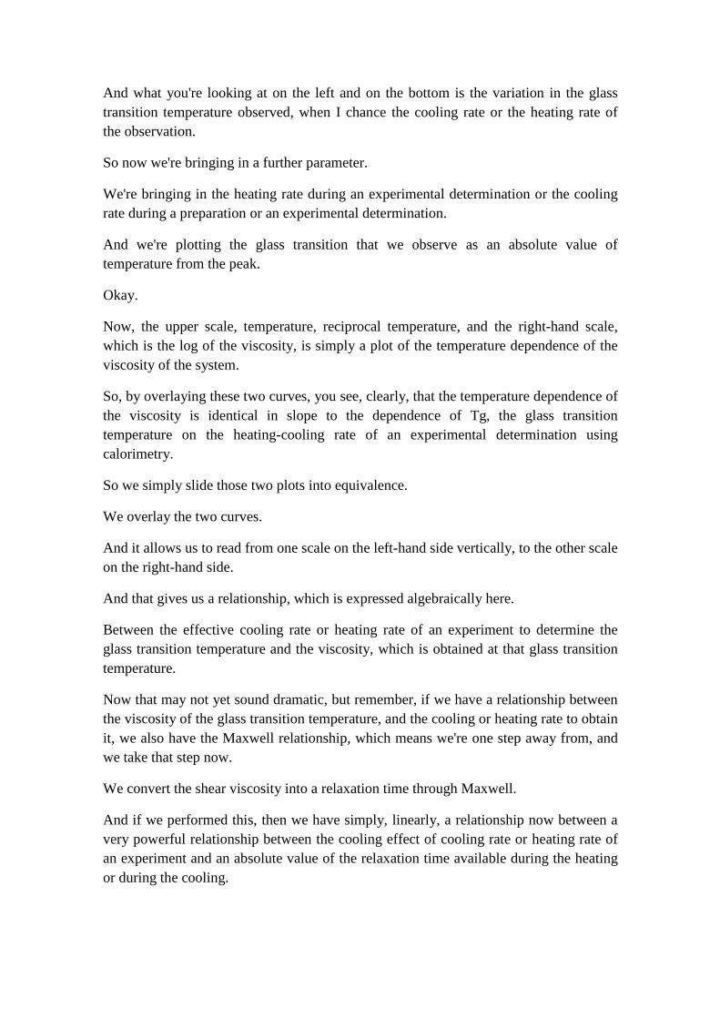
And what you're looking at on the left and on the bottom is the variation in the glass

transition temperature observed, when I chance the cooling rate or the heating rate of

the observation.

So now we're bringing in a further parameter.

We're bringing in the heating rate during an experimental determination or the cooling

rate during a preparation or an experimental determination.

And we're plotting the glass transition that we observe as an absolute value of

temperature from the peak.

Okay.

Now, the upper scale, temperature, reciprocal temperature, and the right-hand scale,

which is the log of the viscosity, is simply a plot of the temperature dependence of the

viscosity of the system.

So, by overlaying these two curves, you see, clearly, that the temperature dependence of

the viscosity is identical in slope to the dependence of Tg, the glass transition

temperature on the heating-cooling rate of an experimental determination using

calorimetry.

So we simply slide those two plots into equivalence.

We overlay the two curves.

And it allows us to read from one scale on the left-hand side vertically, to the other scale

on the right-hand side.

And that gives us a relationship, which is expressed algebraically here.

Between the effective cooling rate or heating rate of an experiment to determine the

glass transition temperature and the viscosity, which is obtained at that glass transition

temperature.

Now that may not yet sound dramatic, but remember, if we have a relationship between

the viscosity of the glass transition temperature, and the cooling or heating rate to obtain

it, we also have the Maxwell relationship, which means we're one step away from, and

we take that step now.

We convert the shear viscosity into a relaxation time through Maxwell.

And if we performed this, then we have simply, linearly, a relationship now between a

very powerful relationship between the cooling effect of cooling rate or heating rate of

an experiment and an absolute value of the relaxation time available during the heating

or during the cooling.

This means that we will be able to plot heating and cooling rates on diagrams of

absolute relaxation time.

And we can compare scanning experiments, dynamic experiments, with static

experiments held at a particular temperature for a particular time.

And you see in the algebra presented here, that you simply transform from a logarithmic

sense, the relationship between the heating and cooling rate, and the viscosity at the

glass transition to one involving the relaxation time at the glass transition.

5-3 Relaxation map, viscosity, shear relaxation time.

Now, let's step back for a moment to recall and to remind ourselves again what we've

already seen once, which is there are different time scales of structural relaxation in

these systems.

We are concerning ourselves in almost everything we will discuss in these days with the

prime or primary relaxation, the so called alpha relaxation in these systems, that which

involves the redistribution of silicon and oxygen bonds, as you'll see in a moment, and

that, which controls the value of the viscosity of the system.

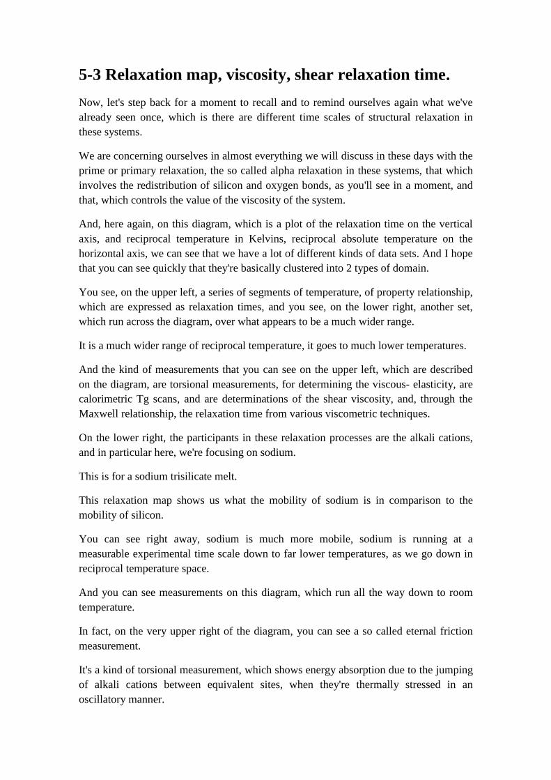
And, here again, on this diagram, which is a plot of the relaxation time on the vertical

axis, and reciprocal temperature in Kelvins, reciprocal absolute temperature on the

horizontal axis, we can see that we have a lot of different kinds of data sets. And I hope

that you can see quickly that they're basically clustered into 2 types of domain.

You see, on the upper left, a series of segments of temperature, of property relationship,

which are expressed as relaxation times, and you see, on the lower right, another set,

which run across the diagram, over what appears to be a much wider range.

It is a much wider range of reciprocal temperature, it goes to much lower temperatures.

And the kind of measurements that you can see on the upper left, which are described

on the diagram, are torsional measurements, for determining the viscous- elasticity, are

calorimetric Tg scans, and are determinations of the shear viscosity, and, through the

Maxwell relationship, the relaxation time from various viscometric techniques.

On the lower right, the participants in these relaxation processes are the alkali cations,

and in particular here, we're focusing on sodium.

This is for a sodium trisilicate melt.

This relaxation map shows us what the mobility of sodium is in comparison to the

mobility of silicon.

You can see right away, sodium is much more mobile, sodium is running at a

measurable experimental time scale down to far lower temperatures, as we go down in

reciprocal temperature space.

And you can see measurements on this diagram, which run all the way down to room

temperature.

In fact, on the very upper right of the diagram, you can see a so called eternal friction

measurement.

It's a kind of torsional measurement, which shows energy absorption due to the jumping

of alkali cations between equivalent sites, when they're thermally stressed in an

oscillatory manner.

But most of the data that you see for the Sodium, on the lower right part of the diagram,

is data obtained from electrical conductivity measurements on silicate melts.

Because sodium is a charge carrier in a sodium trisilicate liquid, it dominates the ionic

conductivity of the system, and therefore, when we measure the electrical conductivity,

we see the behavior of the mobility of sodium.

Now, very importantly on this diagram, if you look closely near the center of the lower

curve or cluster of curves, then you will see that the left-hand side of the sodium curve

is a small segment, in reciprocal space, which is curved. It's not linear.

We would say it's non-Arrheniam.

Yet if you go further to the right hand-side of the same ensemble of data sets, you see, it

looks very linear, on the right-hand side.

So, we have a curve at high temperature, which then switches to a lineaer behavior and

an Arrhenian behavior, as we go to lower temperaure to the right.

Why does this happen?

If you look at the diagram, you will see that where it switches from cruved behavior to

linear behavior I've drawn a vertical line, which runs up to meet the structural relaxation

time, dominated by silicon relaxation.

And where it meets it is essentially a very simple story.

It is the point at which the materials, which are being investigated in the sodium

mobility studies, whether it be diffusion or conductivity, or torsion, it is the point at

which these samples effectively relax, liquify, and therefore it is the temperature above

which these things are behaving as liquids, stable or metastable.

Below this vertical line, as I've drawn it, the materials are being worked on

experimentally in a state, where they stay glassy for the duration of the experiment.

They do not change their structure with temperature.

So, if you will, you are joining a solid state segment of the temperature dependence of

the response of this material, on the right, which is Arrhenian, due to its constant

structure, with one, which is a sum of the responses of relaxation times on the left-hand

side in the liquid state, whose structure, whose liquid structure is permanently and

continuously changing, as I change the temperature, as I change the intensive

parameters in the system, as it must, in order to be in the metastable or a stable

thermodynamic equilibrium.

So, the lower right part of the curve is an isochemical part, it's also an isostructural part

of the curve.

The lower left part of the curve is a isochemical part of the curve, if one has been

careful and no volatility has occurred during the experiment, but it is a, it is not an

isostructural part of the curve.

It is one in, which the structure is changing as a function of temperature, and as a result

of this temperature dependence of the structure, an added parameter, an added degree of

freedom in the variation of the relaxation time with temperature is observed.

And this, simply put, causes the curvature that you see, causes the so-called non-

Arrhenian behavior of the system.

Now, having said all of that, you may look one last time at the top part of the curve, at

the top curve in the diagram.

The top curve in the diagram, to remind you, is the structural relaxation of the system,

dominated by silicon (Si) relaxation, by Si-mobility.

And you can see it is definitely curved.

It is curved over the, virtually, the entire range of its behavior.

And that is simply because, in order to measure the relaxation time of a material.

Where we're looking at the relaxation mode which is controlling viscoelasticity, we

must allow for viscous deformation.

And so, by definition, the structural relaxation times, where we're relaxing, the bulk, by

definition, must show a curvature as a function of temperature, and they do.

In principle, these two curves converge.

You see that right away.

If you would go further up to the lower left of the, temperatures obtained, or such that

this liquid would be stable, that it doesn't reach its boiling point beforehand, then these

two curves, at some point, these two fundamental relaxation times, that of the sodium

(Na) that of the silicon (Si), that must get very, very close.

Remember, we said that the glass transition is not a knife-sharp transition, it can be

approximated to that.

But it really is a range of a few log units of time or of a few tens of degrees, typically, of

temperature, over which the system gradually drifts from liquid to glassy state.

So, you would think that, if I impinge upon this half width of the relaxation of Si and

Na mutually, then I might expect to see further interesting behavior.

And I believe there is evidence that we do.

But very important to remember is that the first transition, I talked about here, going

from non-Arrhenian to Arrhenian is a simple experimental artifact of how long did it

take to do the experiment on sodium mobility in the system, and nothing fundamental to

the nature of relaxation in the system.

Now we hinted a little bit so far as what is really going on, structurally, when we relax

these materials. And when we talk about structural relaxation, you might begin to think,

well, it's essentially the structure, which must relax.

And you'll be right.

The structure of course has many elements, we talked about the structural roles of

cations in these systems and to,

I would say, to the surprise of some and certainly impressing many, for some decades

now, we've known essentially, essentially what's at the heart of the glass transition.

Structural determinations have been made.

Dynamics of bond exchange has been observed, which tells us what is going on at the

glass transition.

You see here, on the plot, which is before you, on the vertical axis, relaxation time.

And on the horizontal axis, reciprocal of the absolute temperature, and in the insert, if

you take a moment to look at it, you see three curves.

They look very, very different in nature, and they correspond to different temperatures

of a single experiment.

You can see at the uppermost curve, that you have individual sharp spikes, which

correspond to species, actually correspond to Q-species, correspond to the number of

non-bridging oxygens on a given individual set of silicate tetrahedra.

These Q-species are in dynamic equilibrium with each other in the melt.

And the purpose of these Nuclear Magnetic Spectroscopic results was to map the

proportions of Q-species in these liquids, at high temperature. And that works fine up to

about 550 degrees Celsius, as you can see.

They can be quantified and the relationships and the reactions between them can be

described. But if you go another 100 degrees higher, to the 650 Celsius, then you see the

curve in the middle there in the stack, which shows that the individual species are no

longer easily distinguished.

You see, more or less, a broad, single peak with a few ups and downs, which basically

demonstrates that these species are beginning to be mobile.

They're beginning to longer be distinguishable on the time scale of the spectroscopic

measurement.

And in the third, the lowermost curve, you see a very sharp single peak.

It's a so called motionally averaged peak.

You've gone through the time scale of relaxation in these systems, and the species now

are exchanging faster than the exposure time, if you will, of the magnetic resonance

spectroscopy, the relaxation time of the nucleus, which is being used to investigate the

equilibria.

So, by obtaining motionally averaged, you've essentially measured a point in time and

temperature, where species exchange is occurring, where bond exchange is occurring.

And the active ingredient in defining the relationship, or the reactions between Q-

species is the exchange of non-bridging oxygens (NBO) between sites around tetrahedra

of silica, such that we have in one point in time, two non-bridging oxygens, and another

point in time, three non bridging oxygens on an individual Si- nucleus.

So, you see, it's really silicon-oxygen bond exchange, which is being motionally

averaged in these NMR- experiments.

And now, look at where they plot in time and temperature.

Remember, that we have the possibility of comparing quantitatively, time and

temperature, whether we're doing scanning experiments, or whether we're doing static

experiments dwell times.

And you can see that, when you plot the results of motional averages of these

spectroscopic experiments, they fall within error, on the line, which describes the

macroscopic relaxation of these systems, (that) which is defined by the temperature

dependence of the viscosity, which yields through the maximal relation, a temperature

dependence of the relaxation time.

That equivalence, if you will, implies that the silicon oxygen bond exchange is

dynamically the mechanism which lies behind the relaxation time of viscous stress of

these systems, of sheer stress, of volume stress. And it is relaxation through viscous

flow.

That is a fairly strong and simple statement. There are other systems, which behave

very, very differently, other chemistry, other than silicates, which behave very, very

differently.

And it implies that these silicate liquids are molecular liquids, relatively, relatively

simple in terms of their dynamics.

Such that the absolute values of their dynamics describe silicon-oxygen bond exchange.

Now this has been further tested beyond that first reconnaisance study.

What you see here is a more detailed comparison of various NMR- experiments, which

have been performed, where relaxation times have been obtained from the species

exchange.

And where they are plotted as data points on top of the relaxation time, which is

determined from a bulk property, the shear of viscosity, through the Maxwell

relationship. And you can see the two curves overlay one another.

It implies that, the silicon-oxygen (Si-O) bond exchange, as the dynamic element

behind viscous relaxation, is valid, not only in low viscosity liquids, such as those on

the lower left of the diagram, but it's also valid, in very, very high viscous liquids.

Those just about to become glasses at the upper right hand part of the diagram.

5-4 The role of dissolved water.

Now, there's one chemical component, very important, in these volcanic systems, which

we've already mentioned.

That is, water, and it turns out that the speciation and the dynamics of the exchange of

the species involved in water dissolution in these systems is fairly simple to describe to

you.

And, it is striking, because it has been measured in many, many different ways.

So, I'd like to use water now as an example of how we can understand better the

dynamics of these systems.

You can see in the diagram in front of you that we have a plot of the weight percent of

water on the vertical axis, versus the total weight percent of water that is in the system,

on the horizontal axis.

The vertical axis is corresponding to the two spectroscopically observed major

components of water dissolved in these systems.

They are on the one hand something, which looks like common water, H20, we call it

molecular water.

And on the other hand, hydroxyl groups, OH groups, which are attached to some cation

sitting within the system.

And this equilibrium between the OH groups, and the molecular water, produces

varying amounts of the two kinds of species, as a function of composition, pressure and

temperature.

What you see in this diagram is the result of quenched experiments from hydrous

rhyolite glasses, high silica glasses, which vary in water content up from about zero to

about six weight percent of water.

And what you see, at the beginning, is that, when you begin to dissolve water in these

glasses and, then quench it after the experiment is done, and look at it in the glassy

state, that you see that we have for the molecular water in these systems a relatively low

value as we begin the dissolution of water.

And most of the water is going in as hydroxyl groups.

But, the two curves are not linear, they cross over as we go to a few weight percent of

water, and we start to have a dominance of molecular water and less of the hydroxyl

groups.

And, these two curves can be viewed as speciation curves.

Remember, they've all been quenched in a similar manner, they have Liquid

compositions, which have widely different viscosities.

Because the dry melts on the left-hand side are very, very viscous.

Whereas those, which contain a lot of water on the right-hand side have a very low

viscosity.

And that's hinted at, at the top of the diagram where you have the double-headed arrow,

which shows high viscosity on the left, low viscosity on the right, high Tg on the left,

low Tg on the right.

So, when looking at these species as afunction of water content, even though the

experiments are done in precisely the same manner, the quench was performed in

precisely the same fashion, we're nevertheless looking at the results of speciation, which

have been quenched onto the fictive temperature curve.

How do we know? We know because there are 2 curves.

There's a set of 2 curves for each of the respective species.

Here one of them is called slow, one of them is called fast.

These are the quench rates involved in determining those two different kinds of data.

You can see here that the fast curves are drawn as solid lines, a speciation, whereas the

slow curves actually exhibit for you the data points, which lie upon them.

And you can see this significant difference in the concentrations of OH and H2O,

depending on whether the quench was slow or was fast.

If sequential's fast, then they get much more OH and much less H2O.

This implies that there is a fictive temperature dependence of the results.

Because the only difference between a slow quench and a fast quench is where the

effective quench rates, in absolute relaxation time, cross the glass transition curve of

what is being quenched, the so-called fictive temperature analysis. And you know that,

if we quench at a fast rate, we will get a higher fictive, or freezing, temperature of the

structure, than if we quench at a slow rate.

So, right away, at a glance, you know what the temperature dependence of the reaction

must be between the hydroxyl groups and the molecular water.

Because a fast quench captures more of the high temperature species, and the fast

quench, here, demonstrates a higher concentration of the hydroxyl groups.

Ergo, the hydroxyl groups are favored at higher temperatures, and the molecular water

is favored at lower temperatures.

Now, if we can quantify precisely where these quench rates are in absolute value.

What relaxation times correspond to them?

And we need one thing more, we need to know the relaxation time temperature curves

of the liquids being investigated and they will vary greatly, because, as you see, the

viscosity varies greatly in the relaxation time and the glass transition varies greatly from

the left to the right.

But if we can plot both of those things, then we can get a matrix of intersections, which

I show to you now.

Where you can see that we have horizontal curves that are called q-curves or quench

curves.

They are described in terms of the absolute values of the rates, 200 degrees Celsius per

minute or per second.

But they're also plotted on a diagram, which is vertically showing you relaxation time

versus reciprocal temperature. And therefore, that reminds you that we can get absolute

values of relaxation time from absolute values of quenched rates.

And this is a reusing.

Now this is the utility of being able to do a fictive temperature analysis based upon

quench rates to produce the materials.

The other curves, which you see here, which cross those horizontal lines, are sample

specific curves.

They're actually calculated curves for the viscosity, and therefore, the relaxation time

through Maxwell, for rhyolitic liquids with 1 and 3 and 5 weight percent of water in

them.

And you can see how much variation there is now. You can see that, if I try to compare

the position of the relaxation time of a melt with one weight percent of water with that

of five, I have a very, very, very large difference.

And this is the fluxing effect of water.

It's this curve of Tg versus water content, which we saw earlier, which drops steeply at

the beginning and then leveled out as we went to higher water contents.

Now the actual data points that we'll obtain from this fictive temperature analysis, then,

are the intersection points of the quenching curves, the two we have available, the fast

and the slow, and the sample curves, which we've parameterized here at one and three

and five weight percent of water, arbitrarily. And when we pick those intersection

points, we can see that that corresponds to a particular temperature for each and every

one.

And those are the fictive temperatures, if you will, in the process of back reaction of the

speciation during the quench.

They are the freezing temperatures of speciation that we obtain in the glasses, on the

bench, afterwards, on which the spectroscopy is performed.

So, we take the speciation data, which corresponds to glasses with one and three and

five weight percent, from the previous diagram of speciation for the fast and for the

slow quench and we assign it to a temperature, which corresponds to the intersection

points, as you see it, on this diagram, classic fictive temperature analysis.

And here you see it must be six data points of course, the two lines crossing three lines

and the six points of intersection, that you see now, are plotted on the upper part of this

diagram.

They're plotted in the form of an equilibrium constant, the natural log of K, which is the

concentration or the activity of H2O, molecular, times oxygens, dry oxygens, as we can

them in the melt, divided by the concentration of the hydroxyl group squared.

And this equilibrium constant, as you can see, within the error bars and over the entire

range of one to five weight percent of water and fast and slow quench, can be fit with a

single line.

That's quite a powerful statement.

It means that, all the complexity and the curved variations of concentrations of species,

that you saw at the outset of this explanation, can be linearized in terms of an

equilibrium constant, as a function of temperature for this reaction.

It means that there's a single value of the enthalpy, which is the slope of the upper

curve, that you see here, which describes the entire reaction, which turns out to be about

25 kilojoules per mole.

I think it's a striking example of the fact that starting out with non-linear variations of

data, starting out with a quench rate dependence, and then, adding in the complexity of

the viscosity-temperature relationships, as a function of water, using that as a corrective

to bring us back to the true value of the temperature dependence of speciation, we

obtain a linear result, with a single value of enthalpy.

Very elegant result.

If you look at the bottom part of the diagram, it's just to give you a hint of what this

means for the absolute values of the concentrations of molecular water and hydroxyl

groups in these melts, as a function of temperature, in this case, reciprocal temperature.

The same as the top part of the diagram.

But you can see the absolute temperatures drawn in the intermediate horizontal axis,

from 1200 to 400 degrees Celsius.

And you can see, at temperatures above 1200 degrees Celsius, we're getting hydroxyl

groups up to 80% of the entire speciation of the water.

So 80% of the water is what we call dissociated water, in the form of individual

hydroxyl groups in these liquids.

And if you go down in a quench, which would bring you down to the lowest on this plot

of around four hundred degrees Celsius, then you end up with less than 40%.

Less than half of the water being maintained as hydroxyl groups and the dominant form

of the water is molecular groups, which are formed during cooling from the hydroxyl

groups.

So, this is a major shift in speciation from 80% to less than 40%, more than a halving of

the relative fraction of hydroxyl groups to molecular water.

Now I want to present you with one more example of how the speciation of water can

be characterized using a physical property determination to calibrate for the glass

transition.

What you see plotted here is pressure versus temperature, and a series of lines on it.

It's, this plot is taken from what you may know, if you've ever investigated fluid

inclusions within rocks.

Here we're going to talk about inclusions that we obtained when we capture a free

volatile phase in a glassy matrix, from quenching of a foamy or a bubbly liquid at high

pressure and high temperature.

Now let me describe carefully what we have in this diagram.

First of all, in the upper right part of the diagram, you see a data point, which we call

chemical equilibration.

That is actually the dwell pressure and temperature, the point of pressure and

temperature at which we held a water-saturated liquid of high viscosity.

I say high viscosity, because it means that the bubbles which are created by starting out

with a powdered sample never actually escape from the liquid.

They're captured as a kind of a foam, or a bubbly liquid, when the material is cooled

down in the quench.

The second point I want to point out to you is the quench, it's a so-called isobaric, or

constant pressure, quench.

It's a line horizontally running from that dwell temperature to the left until we reach

room temperature.

So you have to imagine the quenching of these materials as cooling them down at

constant pressure.

And then once they're cold, relieving the pressure of the sample.

You'll also see at the bottom left, a part of the phase diagram of pure water.

It's called the liquid plus vapor coexistence curve.

And what you see is a line which runs from the lower left and slowly starts to curve up

towards what is termination point.

And that termination point is the critical point of water, beyond which there's no

distinction between a vapor and a liquid.

And we have a high temperature supercritical fluid.

This kind of line describes where a system of the chemistry of water must be, in

pressure and temperature, if we have the coexistence of vapor and liquid in the system.

What you see rising from that liquid plus vapor curve are two linear segments, which

run up and then touch the quench curve, two lines, which run to the upper right. And

those are approximations of isochores, lines of constant volume for the system H20.

We will talk in a moment about inclusions in these systems, which are basically locked

into cages or cavities of a constant size.

And that's why we used isochores or lines of constant volume here.

And the last lines, which you see are schematically drawn in, two estimates of the actual

glass transition temperature, as a function of pressure and temperature in the systems for

fast cooling, and for slow cooling.

Fast to the right, and slow to the left.

So how does it all fit together?

We do our dwell at the chemical equilibration point, upper right.

We cool it down along the horizontal line, isobaric quench.

Then we follow the vertical axis of pressure down until we get to room temperature.

We have a 2-phase system.

We have a liquid at high pressure and temperature.

And we have the gas bubbles inside.

When we cool down along the isobaric quench, at some point, the viscosity of the

liquid, which is falling in temperature, rises so high that we effectively cross the glass

transition.

What does that mean? It means that during the quench, there will no longer be any

structural reaction of the glass to back react as we fall back in temperature. It will lock

in. We will produce a glass during the cooling.

And now we're going to show you how we can get those glass transition temperatures

remotely by looking at the quenched samples.

5-5 The role of dissolved water (cont.).

I said there's two phases.

The glass is produced during the cooling of the liquid, as it comes down in temperature.

But the bubbles, which are inside the liquid, inside the silicate melt are full of water.

And that water, which is cooling at the same time, at the point at which the glass is

produced, at the glass transition, can no longer move in equilibrium as a function of its

volume.

In other words, it can no longer shrink as the sample is cooling down.

There will be a minor elastic shrinkage but the viscous shrinkage, where it really wants

to go to maintain its equilibrium density, is no longer in it's own hands, because the

matrix has decided to freeze up, to lock up, and to hold the volume, the viscous

component of the volume change switched off at the point where the glass is produced.

So, something's gotta give.

What happens is, the pressure in these systems begins to drop.

The volume is locked in, the amount of mass is approximately locked in, diffusion can

be ignored for most of this.

And so if I have a constant amount of mass, a constant amount of volume and I drop the

temperature of a gas, I will drop the pressure.

And so the curve of P and T, pressure and temperature that the inclusion takes

intimately inside of the glass is not the same that the glass takes.

The inclusion, comes down from the chemical equilibrium point, along the horizontal

curve of the isobaric quench until the glass transition is hit.

When you hit the glass transition, when you lock out viscous relaxation of the size of

that bubble, it collapses down an isochore, a constant volume line because its volume is

fixed.

With a minor elastic correction as I refer to again, its volume is essentially fixed.

So it drops down this steep line, which leads from the glass transition down to the liquid

plus vapor curve.

So what do we see when we quench these samples?

We take them out. We do a doubly polished section, we look at it microscopically and

we see inclusions of fluid inside the glass.

And in those fluid inclusions we see two phases.

We see a vapor bubble and we see a liquid portion of the water around the vapor bubble

and wetting to the glass inner surface.

And the presence of those two phases, liquid plus vapor, means we must be on the

liquid plus vapor coexistence line.

And that's what's drawn in the lower left.

So now what we do is we take these samples and we heat them up again.

And when we heat them up, we can watch, as we go along the liquid plus vapor curve

inside these inclusions with a microscope, we can watch the disappearance of one of

these two phases.

And when one of those two phases disappears, the liquid or the vapor, then we are free

to leave this liquid plus vapor coexistence curve.

It is the so-called homogenization temperature, because the entire fluid inclusion

becomes one phase.

And where that occurs is, essentially, where these isochores lift off from the liquid plus

vapor curve.

And so you can see that the homogenization temperature, where we lift off from the

liquid plus vapor curve, is a different, depending upon how the glass was produced,

depending upon where the original glass transition was.

And so, we will get a relatively low value of homogenization temperature from fluid

inclusions, where we see that they have been cooled slowly during the quench.

Because they have a low effective temperature.

And we'll get a relatively high value, where those have been quenched very, very

quickly.

And you know, from the previous example, that, if we have fast and slow quenches, and

we have some kind of evidence for the quantification, that we can start to estimate the

temperature dependence of what's going on in an absolute manner.

So knowing what the isochores of pure water are, knowing where the homogenization

temperatures are, we can find ourselves back on the curve of the quench and we can say

quantitatively, where the glass transition is, where it was experienced on the cooling of

these systems inside of a high pressure vessel at high pressure and high temperature.

The results that we get from such analyses are seen in the following graph.

You see the glass transition temperature obtained from this fluid inclusion analysis, as a

function of composition, in a binary system of composition from a potassium aluminum

silicate, orthoclase to an albite, a sodium aluminum silicate.

And you see the characteristic hallmark of Tg's in binary systems, which is that we don't

get a linear variation of the glass transition.

But we get a deviation from linearity, as we go from one endpoint to the other.

We'll talk about the origins of this later.

But just to drive home the point of how characteristic this is of the glass transition, I've

compared in the next diagram the results of determining the glass transition on the dry

system of orthoclase albite, where you can see on the upper left, the highest temperature

for dry orthoclase, over 900 degrees Celsius.

And then you can see this deviation from additivity, as we call it, as you drive towards

albite, such that the lowest temperature in this system is not actually at albite

composition but it's actually an intermediate temperature in the system.

And I think you'll agree these two curves look very, very, very similar.

Note of course that the absolute temperatures in the fluid inclusion experiments at the

bottom here look very, very different from those in the dry experiments.

Why? Because we have several weight percent of water dissolved in these glasses,

which means that we've shifted their Tg down along that curve that I showed you

earlier, which is a very important point.

Because it means that, despite the fact that we've moved Tg about 400 degrees Celsius,

the characteristics of its variation, as a function of composition, really haven't changed,

between zero weight percent water and 4 to 5 weight percent water in the system.

Now if all of that is true, then it must imply that the quench rate dependence of these

systems also involves a variation in the speciation.

Because, if the speciation is temperature dependent, if I've been able to demonstrate

with fluid inclusions that we can see a shift in fictive temperature, when we have a shift

in the rate at which we quench these fluid inclusions, then there must be a structural

record of the difference.

And what you can see here, subtly, is a slight shift in the relative proportions of the

water, which is dissolved as molecular water, and that which is dissolved as hydroxyl

groups, as a function of the quench rate of these experiments

And, you can see that as the quench rate increases, the hydroxyl groups increase, the

molecular water groups decrease, precisely the direction that we've previously seen in

our experiments.

And here, you see one more very, very interesting feature of this system.

And that is, as we would expect, if the glass transition temperature is the recording

temperature of the speciation of all of these experiments.

And if the glass transition temperature varies nonlinearly in the system due to this

deviation from additivity, then I would expect to see some complexity in the structural

or the spectroscopic results of speciation in these systems.

I would expect to see there, a nonadditivity of the results.

And this is precisely what we see.

And when we look at the concentrations of molecular water and hydroxyl groups in

these samples, we see that there is a deviation from additivity in both cases with

composition.

Such that intermediate values have a higher than linear variation in their molecular

water content.

And the hydroxyl groups are at a minimum in intermediate values of the chemistry.

So here we have something, which on the face of it, looks like a very complex solution

model.

Looks like one whereby the mixing of sodium and potassium is producing some

advantage for the speciation of hydroxyl groups in the system.

If I were to make the mistake of saying that this was an isothermal comparison, then I

would immediately overly complicate the story of speciation in this system.

If I take out the fictive temperature calibration, if I essentially plot all of this versus the

true temperature of speciation equilibration, then what you see is the following diagram,

which is the equilibrium constant for the water speciation reaction as a function of

absolute reciprocal temperature. And it's linear.

If one or two data points, which make life interesting here, but the most important point

is that the high temperature data point you see here is orthoclase plus water, but that the

lowest point, that you see on this diagram, is not albite plus water.

It's an intermediate composition, because of this deviation, such that the lowest values

of the hydroxyl groups are intermediate compositions, and the highest values are

molecular water.

And, therefore, the equilibrium constant expresses itself in terms of its highest value at

an intermediate composition.

See, you literally have a nonlinear plot here or nonlinear background, which has been

linearized by analyzing the fictive temperature.

Exactly as we saw previously but perhaps more impressively.

Now, it also means there is no effective influence of the exchange of sodium for

potassium on a speciation of water in these melts.

So, it means composition in this system, as far as we can measure it, as closely as we

can analyze it, does not matter.

And that everything is a function here of quench temperature.

I'll pause there.

We've taken ourselves much further and much deeper into the phenomena of relaxation

in these systems.

We've seen that we have a wide range of choices, if we want to obtain a quantification

of relaxation in these system.

We can work on a whole range of macroscopic properties, or we have a range of

spectroscopic techniques which we can use to analyze the structure, regardless of

whether we analyze the structure in terms of the fundamental building blocks, the

silicon-oxygen bonds, or whether we analyze the macroscopic properties, which are a

result of the structure, ultimately, we see that the relaxation times that we see for these

systems are one.