Wednesday, Oct. 17, 2012PHYS 3313-001, Fall 2012 Dr. Jaehoon Yu 1 PHYS 3313 – Section 001 Lecture #13 Wednesday, Oct. 17, 2012 Dr. Jaehoon Yu Properties

Wednesday, Oct. 17, 2012 PHYS 3313-001, Fall 2012 Dr. Jaehoon Yu

1

PHYS 3313 – Section 001Lecture #13

Wednesday, Oct. 17, 2012Dr. Jaehoon Yu

• Properties of valid wave functions• Time independent Schrodinger Equation• Expectation Values• Operators – Position, Momentum and Energy• Infinite Potential Well• Finite Potential Well


2

Announcements• Reading assignments

– CH6.1 – 6.7 + the special topic

• Colloquium this week– 4pm, today, Oct. 17, SH101– Drs. Musielak and Fry of UTA

• Please mark your calendar for the Weinberg lecture at 7:30pm, coming Wednesday, Oct. 24!!– Let all of your family and friends know of this.

Wednesday, Oct. 17, 2012 3PHYS 3313-001, Fall 2012 Dr. Jaehoon Yu

Special project #4Show that the wave function Ψ=A[sin(kx-ωt)

+icos(kx-ωt)] is a good solution for the time-dependent Schrödinger wave equation. Do NOT use the exponential expression of the wave function. (10 points)

Determine whether or not the wave function Ψ=Ae-α|x| satisfies the time-dependent Schrödinger wave equation. (10 points)

Due for this special project is Monday, Oct. 22.You MUST have your own answers!

Monday, Oct. 15, 2012 4PHYS 3313-001, Fall 2012 Dr. Jaehoon Yu

Special project #5Show that the Schrodinger equation

becomes Newton’s second law. (15 points)Deadline Monday, Oct. 29, 2012You MUST have your own answers!

Monday, Oct. 15, 2012 5PHYS 3313-001, Fall 2012 Dr. Jaehoon Yu

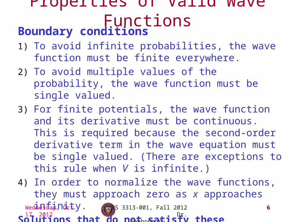
Properties of Valid Wave FunctionsBoundary conditions1) To avoid infinite probabilities, the wave function must be finite

everywhere.2) To avoid multiple values of the probability, the wave function must be

single valued.3) For finite potentials, the wave function and its derivative must be

continuous. This is required because the second-order derivative term in the wave equation must be single valued. (There are exceptions to this rule when V is infinite.)

4) In order to normalize the wave functions, they must approach zero as x approaches infinity.

Solutions that do not satisfy these properties do not generally correspond to physically realizable circumstances.


Time-Independent Schrödinger Wave Equation• The potential in many cases will not depend explicitly on time.• The dependence on time and position can then be separated in

the Schrödinger wave equation. Let,

which yields:

Now divide by the wave function:• The left side of this last equation depends only on time, and the

right side depends only on spatial coordinates. Hence each side must be equal to a constant. The time dependent side is


Ψ x, t( ) =ψ x( ) f t( )

ihψ x( )

∂f t( )∂t

=−h2 f t( )2m

∂2ψ x( )∂x2 +V x( )ψ x( ) f t( )

ih

1

f t( )∂f t( )∂t

=−h2

2m1

ψ x( )∂2ψ x( )∂x2 +V x( )

ih1

f

df

dt=B

We integrate both sides and find:

where C is an integration constant that we may choose to be 0. Therefore

This determines f to be by comparing it to the wave function of a free particle

This is known as the time-independent Schrödinger wave equation, and it is a fundamental equation in quantum mechanics.

Time-Independent Schrödinger Wave Equation(con’t)


ihdf

f∫ = Bdt∫

ln f =

Btih

f t( ) =eBt ih =e−i Bt h

ih

1

f t( )∂f t( )∂t

=E

−

h2

2m

d 2ψ x( )

dx2+V x( )ψ x( ) = Eψ x( )

⇒ ih ln f = Bt +C

=e−iωt ⇒ B h =ω ⇒ B = hω = E

9

Stationary State• Recalling the separation of variables: and with f(t) = the wave function can be

written as:• The probability density becomes:

• The probability distributions are constant in time. This is a standing wave phenomena that is called the stationary state.


Ψ x,t( ) =ψ x( ) f t( )

Ψ x, t( ) =ψ x( )e−iωt

Ψ*Ψ = ψ 2 x( ) eiωte−iωt( ) =ψ 2 x( )

Comparison of Classical and Quantum Mechanics

Newton’s second law and Schrödinger’s wave equation are both differential equations.

Newton’s second law can be derived from the Schrödinger wave equation, so the latter is the more fundamental.

Classical mechanics only appears to be more precise because it deals with macroscopic phenomena. The underlying uncertainties in macroscopic measurements are just too small to be significant due to the small size of the Planck’s constant


10

11

Expectation Values• In quantum mechanics, measurements can only be expressed in terms

of average behaviors since precision measurement of each event is impossible

• The expectation value is the expected result of the average of many measurements of a given quantity. The expectation value of x is denoted by <x>.

• Any measurable quantity for which we can calculate the expectation value is called a physical observable. The expectation values of physical observables (for example, position, linear momentum, angular momentum, and energy) must be real, because the experimental results of measurements are real.

• The average value of x is


x =N1x1 + N2x2 + N3x3 + N4x4 +L

N1 + N2 + N3 + N4 +L=

Nixii∑

Nii∑

Continuous Expectation Values• We can change from discrete to

continuous variables by using the probability P(x,t) of observing the particle at a particular x.

• Using the wave function, the expectation value is:

• The expectation value of any function g(x) for a normalized wave function:


x =xP x( )dx

−∞

+∞

∫P x( )dx

−∞

+∞

∫

x =xΨ x,t( )* Ψ x,t( )dx

−∞

+∞

∫Ψ x,t( )* Ψ x,t( )dx

−∞

+∞

∫

g x( ) = Ψ x,t( )* g x( )Ψ x,t( )dx−∞

+∞

∫

Momentum Operator• To find the expectation value of p, we first need to represent p in

terms of x and t. Consider the derivative of the wave function of a free particle with respect to x:

With k = p / ħ we have

This yields

• This suggests we define the momentum operator as .• The expectation value of the momentum is


∂Ψ∂x=∂

∂xei kx−ωt( )⎡⎣ ⎤⎦=

∂Ψ∂x=

p Ψ x,t( )⎡⎣ ⎤⎦=

p =−ih

∂∂x

p =

ikei kx−ωt( ) =ikΨ

ip

hΨ

−ih

∂Ψ x,t( )

∂x

Ψ* x, t( )−∞

+∞

∫ pΨ x, t( )dx = −ih Ψ * x, t( )

−∞

+∞

∫∂Ψ x, t( )

∂xdx

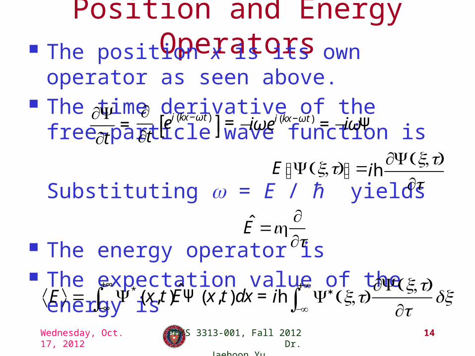
Position and Energy Operators The position x is its own operator as seen above. The time derivative of the free-particle wave function

is

Substituting ω = E / ħ yields

The energy operator is The expectation value of the energy is


14

∂Ψ∂t=

E Ψ x,t( )⎡⎣ ⎤⎦=

E =ih

∂∂t

E =

∂∂tei kx−ωt( )⎡⎣ ⎤⎦= −iωei kx−ωt( ) = −iωΨ

ih∂Ψ x,t( )

∂t

Ψ* x, t( )−∞

+∞

∫ EΨ x, t( )dx = ih Ψ* x,t( )

−∞

+∞

∫∂Ψ x,t( )

∂tdx

Infinite Square-Well Potential• The simplest such system is that of a particle trapped in a

box with infinitely hard walls that the particle cannot penetrate. This potential is called an infinite square well and is given by

• The wave function must be zero where the potential is infinite.

• Where the potential is zero inside the box, the Schrödinger wave equation becomes where

.• The general solution is .


V x( ) =∞ x≤0,x≥L0 0 < x< L

⎧⎨⎩

d 2ψdx2 =−

2mEh2 ψ

k = 2mE h2

ψ x( ) = Asin kx + Bcoskx

=−k2ψ

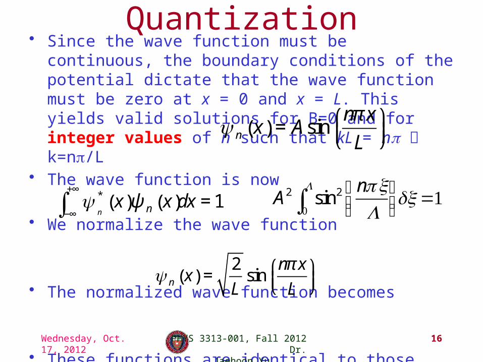
Quantization• Since the wave function must be continuous, the boundary conditions

of the potential dictate that the wave function must be zero at x = 0 and x = L. This yields valid solutions for B=0 and for integer values of n such that kL = nπ k=nπ/L

• The wave function is now

• We normalize the wave function

• The normalized wave function becomes

• These functions are identical to those obtained for a vibrating string with fixed ends.


ψ n x( ) = Asinnπ x

L⎛⎝⎜

⎞⎠⎟

ψn

* x( )ψ n x( )−∞

+∞

∫ dx = 1

ψ n x( ) =2

Lsin

nπ x

L⎛⎝⎜

⎞⎠⎟

A2 sin2nπxL

⎛⎝⎜

⎞⎠⎟0

L

∫ dx=1

Documents

Wednesday, Oct. 17, 2012PHYS 3313-001, Fall 2012 Dr. Jaehoon Yu 1 PHYS 3313 – Section 001 Lecture #13 Wednesday, Oct. 17, 2012 Dr. Jaehoon Yu Properties