Embed Size (px)
Citation preview

Monday, Oct. 15, 2012 PHYS 3313-001, Fall 2012 Dr. Jaehoon Yu
1
PHYS 3313 – Section 001Lecture #12
Monday, Oct. 15, 2012Dr. Jaehoon Yu
• The Schrödinger Wave Equation• Time-Independent Schrödinger Wave Equation• Probability Density• Wave Function Normalization• Expectation Values• Operators – Position, Momentum and Energy

Monday, Oct. 15, 2012 PHYS 3313-001, Fall 2012 Dr. Jaehoon Yu
2
Announcements• Reminder Homework #4
– End of chapter problems on CH5: 8, 10, 16, 24, 26, 36 and 47
– Due: This Wednesday, Oct. 17
• Reading assignments– CH6.1 – 6.7 + the special topic
• Colloquium this week– 4pm, Wednesday, Oct. 17, SH101– Drs. Musielak and Fry of UTA

Monday, Oct. 15, 2012 3PHYS 3313-001, Fall 2012 Dr. Jaehoon Yu

Special project #5Prove that the wave function Ψ=A[sin(kx-ωt)
+icos(kx-ωt)] is a good solution for the time-dependent Schrödinger wave equation. Do NOT use the exponential expression of the wave function. (10 points)
Determine whether or not the wave function Ψ=Ae-α|x| satisfy the time-dependent Schrödinger wave equation. (10 points)
Due for this special project is Monday, Oct. 22.You MUST have your own answers!
Monday, Oct. 15, 2012 4PHYS 3313-001, Fall 2012 Dr. Jaehoon Yu
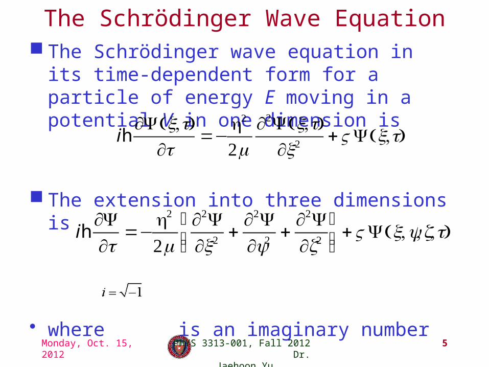
The Schrödinger Wave Equation The Schrödinger wave equation in its time-dependent
form for a particle of energy E moving in a potential V in one dimension is
The extension into three dimensions is
• where is an imaginary number
Monday, Oct. 15, 2012 5PHYS 3313-001, Fall 2012 Dr. Jaehoon Yu
ih∂Ψ x,t( )
∂t=−
h2
2m∂2Ψ x,t( )
∂x2 +VΨ x,t( )
ih∂Ψ∂t
=−h2
2m∂2Ψ∂x2 +
∂2Ψ∂y2 +
∂2Ψ∂z2
⎛
⎝⎜⎞
⎠⎟+VΨ x,y,z,t( )
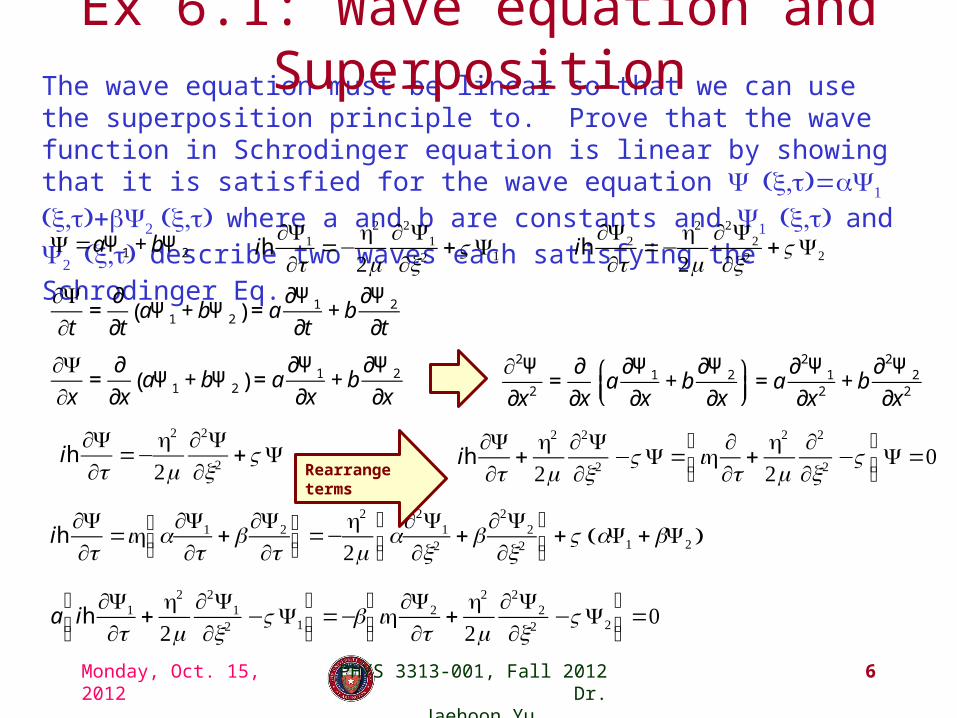
The wave equation must be linear so that we can use the superposition principle to. Prove that the wave function in Schrodinger equation is linear by showing that it is satisfied for the wave equation Ψ ( , )= Ψx t a 1 ( , )+ Ψx t b 2 ( , ) x t where a and b are constants and Ψ1 ( , ) x t and Ψ2 ( , ) x t describe two waves each satisfying the Schrodinger Eq.
Ex 6.1: Wave equation and Superposition
Monday, Oct. 15, 2012 6PHYS 3313-001, Fall 2012 Dr. Jaehoon Yu
Ψ =aΨ1 + bΨ 2
∂Ψ∂t
=∂
∂taΨ1 + bΨ 2( ) = a
∂Ψ1
∂t+ b
∂Ψ 2
∂t
∂Ψ∂x
=∂
∂xaΨ1 + bΨ 2( ) = a
∂Ψ1
∂x+ b
∂Ψ 2
∂x∂2Ψ
∂x2=
∂
∂xa
∂Ψ1
∂x+ b
∂Ψ 2
∂x⎛⎝⎜
⎞⎠⎟
= a∂2Ψ1
∂x2+ b
∂2Ψ 2
∂x2
ih∂Ψ∂t
=−h2
2m∂2Ψ∂x2 +VΨ
ih∂Ψ∂t
=ih a∂Ψ1
∂t+b
∂Ψ2
∂t⎛⎝⎜
⎞⎠⎟=−
h2
2ma∂2Ψ1
∂x2 +b∂2Ψ2
∂x2
⎛
⎝⎜⎞
⎠⎟+V aΨ1 +bΨ2( )
a ih
∂Ψ1
∂t+
h2
2m∂2Ψ1
∂x2 −VΨ1
⎛
⎝⎜⎞
⎠⎟=−b ih
∂Ψ2
∂t+
h2
2m∂2Ψ2
∂x2 −VΨ2
⎛
⎝⎜⎞
⎠⎟=0
ih∂Ψ1
∂t=−
h2
2m∂2Ψ1
∂x2 +VΨ1 ih∂Ψ2
∂t=−
h2
2m∂2Ψ2
∂x2 +VΨ2
Rearrange terms
ih∂Ψ∂t
+h2
2m∂2Ψ∂x2 −VΨ = ih
∂∂t
+h2
2m∂2
∂x2 −V⎛
⎝⎜⎞
⎠⎟Ψ =0
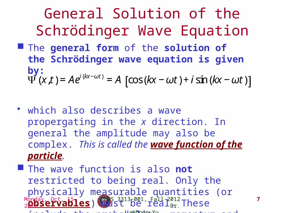
General Solution of the Schrödinger Wave Equation
The general form of the solution of the Schrödinger wave equation is given by:
• which also describes a wave propergating in the x direction. In general the amplitude may also be complex. This is called the wave function of the particle.
The wave function is also not restricted to being real. Only the physically measurable quantities (or observables) must be real. These include the probability, momentum and energy.
Monday, Oct. 15, 2012 7PHYS 3313-001, Fall 2012 Dr. Jaehoon Yu
Ψ x, t( ) = Aei kx−ωt( ) = A cos kx −ωt( ) + i sin kx −ωt( )⎡⎣ ⎤⎦

Show that Aei(kx-ωt) satisfies the time-dependent Schrodinger wave Eq. Ex 6.2: Solution for wave equation
Monday, Oct. 15, 2012 8PHYS 3313-001, Fall 2012 Dr. Jaehoon Yu
Ψ =Aei kx−ωt( )
∂Ψ∂x
=∂
∂xAei kx−ωt( )
( ) = iAkei kx−ωt( ) = ikΨ
ih∂Ψ∂t
=ih −iωΨ( ) =hωΨ =−h2
2m−k2Ψ( ) +VΨ
∂Ψ∂t
=∂
∂tAei kx−ωt( )
( ) = −iAωei kx−ωt( ) = −iωΨ
∂2Ψ
∂x2=
∂
∂xikΨ( ) = ik
∂
∂xΨ( ) = ik iAkei kx−ωt( )
( ) = −Ak2ei kx−ωt( ) = −k2Ψ
hω −
h2k2
2m−V
⎛
⎝⎜⎞
⎠⎟Ψ = 0
E −p2
2m−V =0
The Energy: E =hf =h
ω2π
⎛⎝⎜
⎞⎠⎟=hω = E −
p2
2m−V
⎛
⎝⎜⎞
⎠⎟= 0
The wave number: k =
2πλ
=2πh p
=2π ph
=ph The momentum: p =hk
From the energy conservation: E =K +V =p2
2m+V
So Aei(kx-ωt) is a good solution and satisfies Schrodinger Eq.
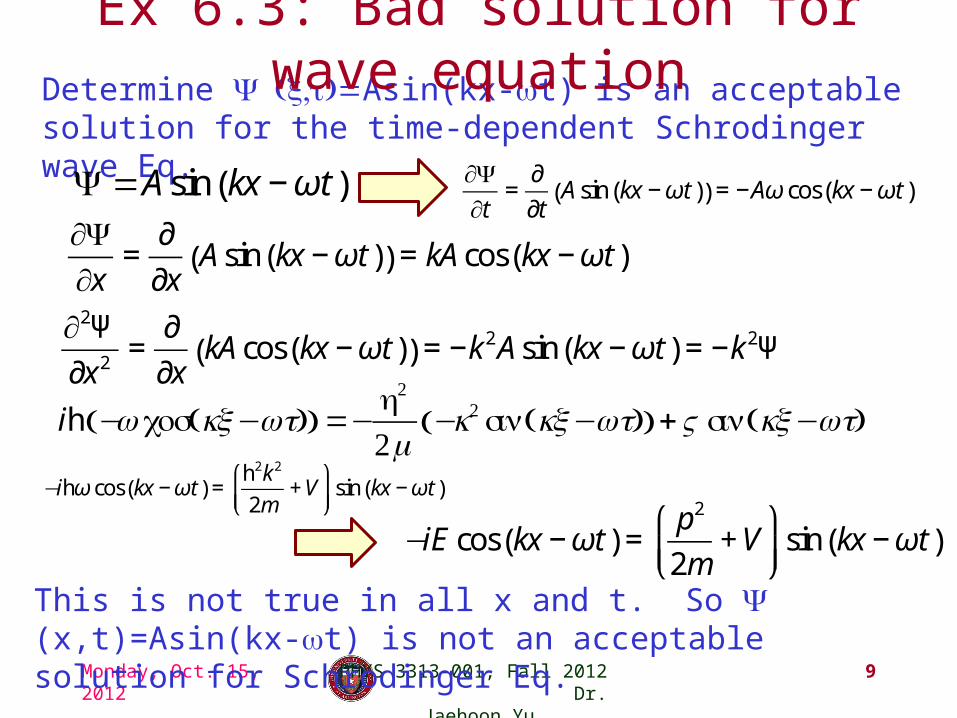
Determine Ψ ( , )=x t Asin(kx-ωt) is an acceptable solution for the time-dependent Schrodinger wave Eq.
Ex 6.3: Bad solution for wave equation
Monday, Oct. 15, 2012 9PHYS 3313-001, Fall 2012 Dr. Jaehoon Yu
Ψ =Asin kx −ωt( )∂Ψ∂x
=∂
∂xAsin kx −ωt( )( ) = kAcos kx −ωt( )
ih −ω cos kx−ωt( )( ) =−
h2
2m−k2 sin kx−ωt( )( ) +Vsin kx−ωt( )
∂Ψ∂t
=∂
∂tAsin kx −ωt( )( ) = −Aω cos kx −ωt( )
∂2Ψ
∂x2=
∂
∂xkAcos kx −ωt( )( ) = −k2Asin kx −ωt( ) = −k2Ψ
This is not true in all x and t. So Ψ (x,t)=Asin(kx-ωt) is not an acceptable solution for Schrodinger Eq.
−ihω cos kx −ωt( ) =
h2k2
2m+V
⎛
⎝⎜⎞
⎠⎟sin kx −ωt( )
−iE cos kx −ωt( ) =p2
2m+V
⎛
⎝⎜⎞
⎠⎟sin kx −ωt( )

Normalization and Probability The probability P(x) dx of a particle being between x
and X + dx was given in the equation
• Here Ψ* denotes the complex conjugate of Ψ The probability of the particle being between x1 and x2 is
given by
The wave function must also be normalized so that the probability of the particle being somewhere on the x axis is 1.
Monday, Oct. 15, 2012 10PHYS 3313-001, Fall 2012 Dr. Jaehoon Yu
P x( )dx=Ψ* x,t( )Ψ x,t( )dx
P = Ψ*Ψdxx1
x2
∫
Ψ* x, t( )Ψ x, t( )dx−∞
+∞
∫ = 1

Consider a wave packet formed by using the wave function that Ae-α| |x , where A is a constant to be determined by normalization. Normalize this wave function and find the probabilities of the particle being between 0 and 1/α, and between 1/α and 2/α.
Ex 6.4: Normalization
Monday, Oct. 15, 2012 11PHYS 3313-001, Fall 2012 Dr. Jaehoon Yu
Ψ =Ae−α x
Ψ*
−∞
+∞
∫ Ψdx = Ae−α x( )
*Ae−α x
( )−∞
+∞
∫ dx =Probability density A*e−α x
( ) Ae−α x( )
−∞
+∞
∫ dx=
= A2e−2α x
−∞
+∞
∫ dx =
Ψ = αe−α x A = α Normalized Wave Function
2A2
−2αe−2α x
0
+∞
= 0 +A2
α= 12 A2e−2α x
0
+∞
∫ dx=

Using the wave function, we can compute the probability for a particle to be with 0 to 1/α and 1/α to 2/α.
Ex 6.4: Normalization, cont’d
Monday, Oct. 15, 2012 12PHYS 3313-001, Fall 2012 Dr. Jaehoon Yu
Ψ = αe−α x
P = Ψ*
0
1 α
∫ Ψdx=
For 0 to 1/α:
For 1/α to 2/α:
How about 2/α:to ∞?
αe−2α x
0
1 α
∫ dx =α−2α
e−2α x
0
1 α
= −1
2e−2 −1( ) ≈ 0.432
P = Ψ*
1 α
2 α
∫ Ψdx= αe−2α x
1 α
2 α
∫ dx =α−2α
e−2α x
1 α
2 α
= −1
2e−4 − e−2( ) ≈0.059