10.1

ECE 410 DIGITAL SIGNAL PROCESSING D. Munson University of Illinois Chapter 10 Classes of Digital Filters FIR – Finite impulse response; {hn} finite in length IIR – Infinite impulse response; {hn} infinite in length FIR Filter Structures hn = a0, a1, a2, … , aN–1, 0, 0, …{ }

⇒ H(z) = ann= 0

N –1∑ z–n

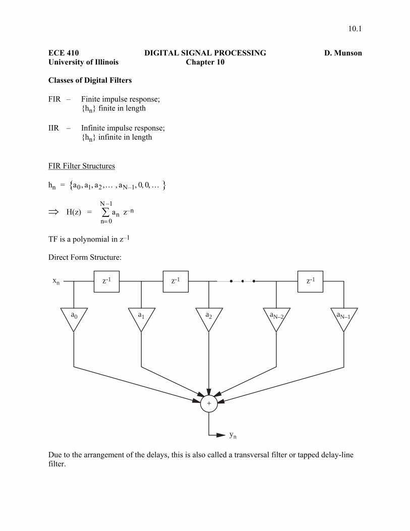
TF is a polynomial in z–1 Direct Form Structure:

z-1z-1 z-1

a0

xn

yn

a1 a2 aN–2 aN–1

+

Due to the arrangement of the delays, this is also called a transversal filter or tapped delay-line filter.

10.2

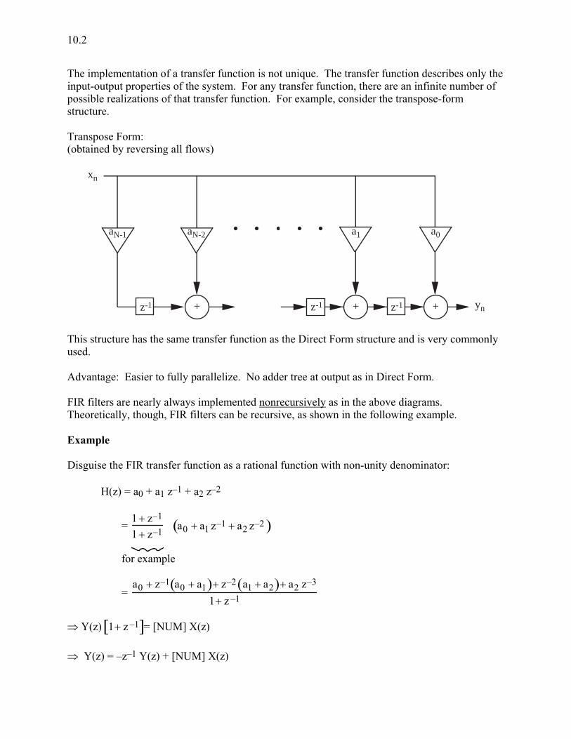
The implementation of a transfer function is not unique. The transfer function describes only the input-output properties of the system. For any transfer function, there are an infinite number of possible realizations of that transfer function. For example, consider the transpose-form structure. Transpose Form: (obtained by reversing all flows)

z-1 z-1

a0a1aN-2aN-1

xn

+ ynz-1 + +

This structure has the same transfer function as the Direct Form structure and is very commonly used. Advantage: Easier to fully parallelize. No adder tree at output as in Direct Form. FIR filters are nearly always implemented nonrecursively as in the above diagrams. Theoretically, though, FIR filters can be recursive, as shown in the following example. Example Disguise the FIR transfer function as a rational function with non-unity denominator: H(z) = a0 + a1 z–1 + a2 z–2

= 1 + z–1

1 + z–1 a0 + a1 z–1 + a2 z–2( )

for example

= a0 + z–1 a0 + a1( )+ z–2 a1 + a2( )+ a2 z–3

1+ z –1

⇒ Y(z) 1+ z –1[ ]= [NUM] X(z) ⇒ Y(z) = –z–1 Y(z) + [NUM] X(z)

10.3

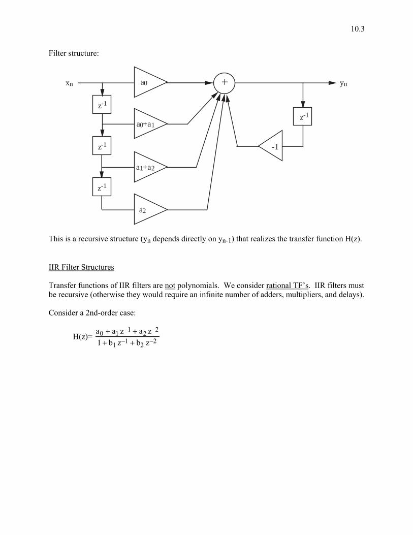
Filter structure:

z-1

a0

a0+a1

a1+a2

a2

-1

z-1

ynxn

z-1

z-1

+

This is a recursive structure (yn depends directly on yn-1) that realizes the transfer function H(z). IIR Filter Structures Transfer functions of IIR filters are not polynomials. We consider rational TF’s. IIR filters must be recursive (otherwise they would require an infinite number of adders, multipliers, and delays). Consider a 2nd-order case:

H(z)= a0 + a1 z–1 + a2 z–2

1 + b1 z–1 + b2 z–2

10.4

Direct Form 1 structure:

a0 ynxn

z-1

z-1

a1

a2

z-1

z-1

+

- b1

- b2

Can also implement using a Direct Form 2 structure:

z–1

z–1

a0

a1

a2

–b1

–b2

xn yn+ +

We showed earlier that this structure has the same transfer function H(z) as the Direct Form 1 structure. IIR filters are always recursive. FIR filters are implemented in nonrecursive form. Implementation of Higher-Order Digital Filters (Order of filter = max {degree (Num), degree (Den)} = # delays required for a Direct Form 2 implementation) High-order direct-form filters can have large error at the output due to multiplication roundoff. Also, the actual Hd(ω) may deviate considerably from the desired due to coefficient rounding.

10.5

Cascaded or parallel second-order sections exhibit smaller error than direct form. Also, splitting into lower-order sections can make filter easier to parallelize (e.g., second-order filter on a chip). Cascade Form:

H(z) = a0 + a1 z–1 +…+ aN z–N

1 + b1 z–1 +…+ bN z–N

= a0 zN + a1zN–1 +… + aNzN + b1 zN–1 + …+ bN

Write as:

H(z) = a0 z – ziz – pii=1

N∏

Since ai, bi are real, if pi is complex, there must be some pk = pi

∗ . Pair up poles and zeros so that (assume N is even)

H(z) = a0 Hi(z)i=1

N /2∏

where

Hi(z) =

(z – zk) (z – z )(z – pm) (z – pn)

is a second-order filter section with z = zk

∗ and pn = pm∗ .

Pair up complex conjugates so that all multiplier coefficients of the second-order sections are real, so filter can use real arithmetic. (If zk is real, then pair up with any real z ; similarly for poles.) For instance, suppose you factor H(z) and find two poles are pm = 1 + j, pn = 1 – j Then pair these poles together in the same Hi(z) so that:

Hi(z) =

(z – zk) (z – z )z – (1+ j)[ ] z – (1 – j)[ ]

=

(z – zk ) (z – z )z2 – z – j z – z + j z + (1+ j) (1– j)

10.6

=(z – zk)(z – z )

z2 – 2z + 2

real filter coeffs. H(z) implemented in cascade form looks like:

X(z) Y(z)a0 H1(z) H2(z) H (z)N2

…

where each Hi(z) is a second-order section. If N is odd, then one of the above sections will be a first-order filter. Parallel Form: Expand H(z) in a PFE:

H(z)

z =

Az

+ B1

z – p1 + … +

BNz – pN

⇒ H(z) = A + B1 z

z – p1 + … +

BN zz – pN

Again, pair up complex poles. If pk= p

∗ then know that Bk = B∗ so that

Bk z

z – pk +

B zz – p

=

B∗ zz – p∗ +

B zz – p

=

B∗ z(z – p ) + B z(z – p∗)z – p∗( )(z – p )

=

z2 B∗ + B( )– z B∗ p + B p∗( )z2 – z p∗ + p( )+ p p∗

coeffs. are all real Parallel realization (assume N is even):

10.7

H(z) = A + Hi(z)i=1

N /2∑

where

Hi(z) = a1i z2 + a2iz

z2 + b1i z + b2i

= a1i + a2i z–1

1 + b1i z–1 + b2i z–2

are second-order sections. Note that, due to the form of the numerator, each of these second-order sections requires one fewer multiplication than for cascade form. Implementation:

X(z)

H1(z)

H2(z)

HN/2(z)

A

Y(z).

.

.

.

+

If N is odd, then one of the above filter sections will be first-order.

10.8

Example

Suppose H(z) = z4 +1

z4 –1

16

.

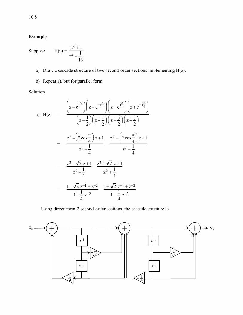
a) Draw a cascade structure of two second-order sections implementing H(z). b) Repeat a), but for parallel form.

Solution

a) H(z) = z – e

jπ4

z – e

–j π4

z + e

jπ4

z + e

– j π4

z – 12

z + 1

2

z – j

2

z + j

2

= z2 – 2 cos

π4

z +1

z2 –14

z2 + 2 cos

π4

z +1

z2 + 14

= z2 – 2 z +1

z2 –14

z2 + 2 z + 1

z2 + 14

= 1 – 2 z–1 + z–2

1– 14

z–2

1+ 2 z–1 + z–2

1 + 14

z–2

Using direct-form-2 second-order sections, the cascade structure is

14

z–1

14

xn yn

√2–

z–1

z–1

z–1

√2

–

10.9

b) H(z)

z =

z4 +1

z z – 12

z + 1

2

z – j

2

z + j

2

= Az

+ B1

z – 12

+ B2

z + 12

+ B3

z – j2

+ B4

z + j2

⇒ H(z) = A +

B1 z

z – 12

+ B2 z

z + 12

+ B3 z

z – j2

+ B4 z

z + j2

= A + B1 + B2( ) z2 +

12

B1 – B2( ) z

z – 12

z + 1

2

+ B3 + B4( ) z2 +

j2

B3 – B4( ) z

z – j2

z + j

2

= A + B1 + B2( )+

12

B1 – B2( ) z–1

1 – 14

z–2 +

B3 + B4( )+j2

B3 – B4( )z–1

1+ 14

z–2

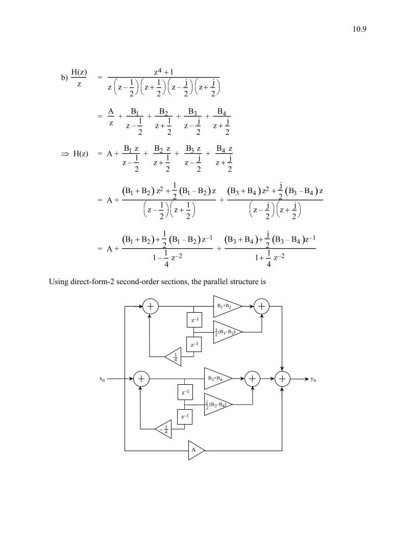
Using direct-form-2 second-order sections, the parallel structure is

yn

A

xn

14

B1+B2

z–1

z–1

(B1–B2)12

14

B3+B4

z–1

z–1

(B3–B4)j2

–

10.10

Note: In this diagram, A and the Bi are the coefficients in the PFE. B4 is the complex conjugate of B3, so all multiplier values are real. Both the cascade and parallel structures will implement the original transfer function H(z), and will generally do so with less error due to finite register length than a 4th-order direct-form implementation. Generalized Linear Phase Filters Linear Versus Generalized Linear Phase Will say Hd(ω) is linear phase if Hd(ω) = Hd(ω) e–jωM nonnegative Fact: A digital filter doesn’t usually have exactly linear phase. But is easy to design FIR filters having what we will call generalized linear phase. Are two types. Type 1: Hd(ω) = R(ω) e–jωM ↑ real, but not nonnegative Type 2: Hd(ω) = R(ω) ej(α–ωM) with α ≠ 0. We will see that generalized linear phase corresponds to having linear phase over the passband. FIR Versus IIR Filters Advantage of FIR: Easy to design with generalized linear phase (linear phase over passband). Advantage of IIR: Can’t have exactly linear phase or generalized linear phase, but IIR can often meet Hd(ω) specification with a much lower order filter. Generalized Linear Phase Property of FIR Filters

10.11

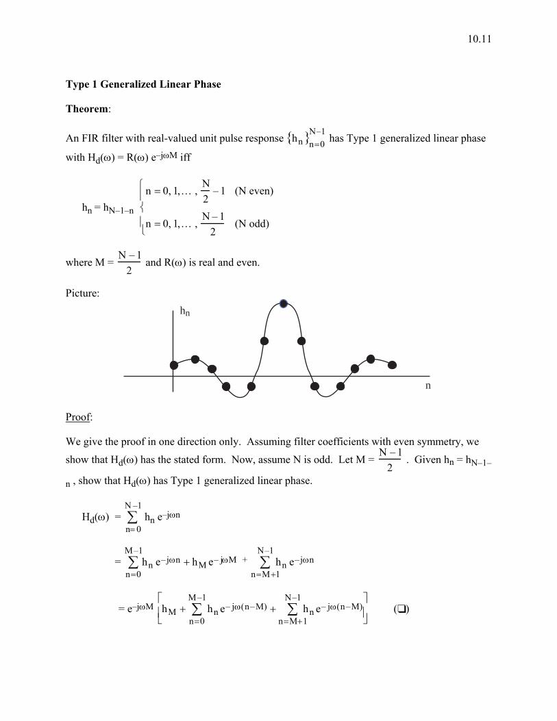
Type 1 Generalized Linear Phase Theorem: An FIR filter with real-valued unit pulse response hn{ }n=0

N–1 has Type 1 generalized linear phase

with Hd(ω) = R(ω) e–jωM iff

hn = hN–1–n n = 0, 1, … ,

N2

– 1 (N even)

n = 0, 1, … ,N – 1

2(N odd)

where M = N – 1

2 and R(ω) is real and even.

Picture:

n

hn

Proof: We give the proof in one direction only. Assuming filter coefficients with even symmetry, we

show that Hd(ω) has the stated form. Now, assume N is odd. Let M = N – 1

2 . Given hn = hN–1–

n , show that Hd(ω) has Type 1 generalized linear phase.

Hd(ω) = n= 0

N –1∑ hn e–jωn

= hn e–jωn + hM e– jωMn=0

M–1∑ + hn e–jωn

n=M+1

N–1∑

= e–jωM hM + hn e– jω(n–M)n=0

M–1∑ + hn e– jω(n–M)

n=M+1

N–1∑

(❑ )

10.12

Now, making the change of variable n = N–1–k and using M = N – 1

2, the second sum in (❑ ) can

be written as

hN–1–k e– jω (M–k)k= M–1

0∑

Thus,

Hd(ω) = e–jωM hM + hn e– jω (n–M) + hN–1–n e– jω(M–n)( )n=0

M–1∑

(❑❑ )

and using hN–1–n = hn, we have

Hd(ω) = e–jωM hM + 2 hn cosω(n – M)n=0

M–1∑

∆=

R(ω) ~ real valued

Note: Hd(ω) = R(ω)

∠Hd(ω) = –ωM ω : R(ω) > 0{ }

–ωM ± π ω : R(ω) < 0{ }

(∆)

↑ –1 = e±jπ (∆) ⇒ phase is linear except where R(ω) changes sign, in which case the phase jumps by π. This implies that a generalized linear-phase filter has linear phase over the passband since

R(ω) can’t change sign inpassband since |Hd(ω)| = |R(ω)|≠ 0 in passband

–π π ω

|Hd(ω)| = |R(ω)|

10.13

To prove the theorem in the other direction, start with Hd(ω) = R(ω) e–jωM . ↑ real and even Then can show hn = hN–1–n .

Note: If N is even then we still take M = N – 1

2 and the proof is nearly the same as above.

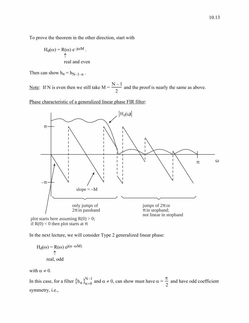
Phase characteristic of a generalized linear phase FIR filter:

plot starts here assuming R(0) > 0;if R(0) < 0 then plot starts at π

π

–π

π ω

slope = –M

| |Hd(ω)

jumps of 2π orπ in stopband;not linear in stopband

only jumps of2π in passband

In the next lecture, we will consider Type 2 generalized linear phase: Hd(ω) = R(ω) ej(α–ωM) ↑ real, odd with α ≠ 0. In this case, for a filter hn{ }n=0

N–1 and α ≠ 0, can show must have α = π2

and have odd coefficient

symmetry, i.e.,

10.14

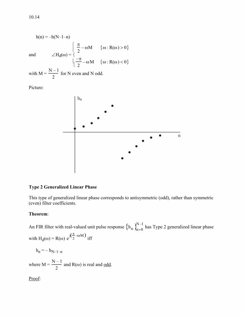
h(n) = –h(N–1–n)

and ∠Hd(ω) =

π2

– ωM ω : R(ω) > 0{ }

–π2

– ωM ω : R(ω) < 0{ }

with M = N – 1

2 for N even and N odd.

Picture:

hn

n

Type 2 Generalized Linear Phase This type of generalized linear phase corresponds to antisymmetric (odd), rather than symmetric (even) filter coefficients. Theorem: An FIR filter with real-valued unit pulse response n=0

N –1hn{ } has Type 2 generalized linear phase

with Hd(ω) = R(ω) ej(π

2–ωM)

iff hn = – hN–1–n

where M = N – 1

2 and R(ω) is real and odd.

Proof:

10.15

We give the proof in one direction only. Assuming filter coefficients with odd symmetry, we

show that Hd(ω) has the stated form. Now, assuming N is odd and taking M = N – 1

2 we have

from before:

Hd(ω) = e–jωM hM + (hn e– jω(n–M) + hN–1–n e –jω(M–n) )n=0

M–1∑

(❑❑ )

Given that hn = – hN–1–n we must have hM = 0. Can see this pictorially:

hn

M n

Obviously, we cannot have odd coefficient symmetry unless hM = 0. Now, setting hM = 0 and using hN–1–n = – hn in (❑❑ ), we have

Hd(ω) = e–jωM hnn=0

M–1∑ e– jω(n–M) – ejω(n–M)( )

= e–jωM (–j2) hnn=0

M–1∑ sinω(n–M)

= ej(π

2–ωM)

–2 hn sinω(n – M)n=0

M–1∑

= R(ω), which is real and odd So, for the antisymmetric coefficient case, we have Hd(ω) = R(ω) , but now R(ω) is a linear combination of sines (odd) instead of cosines (even) and

∠Hd(ω) =

π2

– ωM {ω : R(ω) > 0}

–π2

– ωM {ω : R(ω) < 0}

10.16

To prove the theorem in the other direction, start with

Hd(ω) = R(ω) ej π

2–ωM

↑ real and odd Then can show hn = – hN–1–n .

Note: If N is even instead of odd, we still take M = N – 1

2 and the proof is nearly the same as

above. Example Determine whether a filter with the unit-pulse response {hn} = {1, –1, 1} ↑ has generalized linear phase, and if so, whether it has linear phase. Note: Linear phase ⇒ generalized linear phase, but not vice versa. Solution hn is symmetric about its midpoint ⇒ Have Type 1 generalized linear phase. To check whether we have linear phase, we must find the phase of the frequency response: Hd(ω) = 1 – e–jω + e–j2ω = e–jω (ejω – 1 + e–jω) ↑ e–jωM where M = 1 in this example = e–jω (2 cosω–1) R(ω) We see that R(ω) changes sign on –π < ω < π. Thus, we know that this filter does not have linear phase. Let’s find the phase:

∠Hd(ω) = –ω {ω : 2 cosω – 1 > 0}

–ω + π {ω : 2 cosω – 1 < 0}

10.17

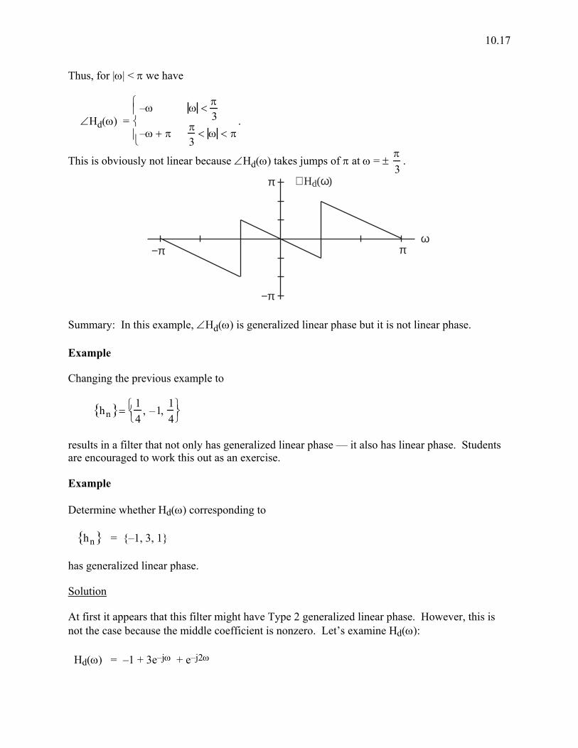
Thus, for |ω| < π we have

∠Hd(ω) = –ω ω < π

3–ω + π π

3< ω < π

.

This is obviously not linear because ∠Hd(ω) takes jumps of π at ω = ± π3

.

π

−π

−π πω

∠ Hd(ω)

Summary: In this example, ∠Hd(ω) is generalized linear phase but it is not linear phase. Example Changing the previous example to

hn{ }=14

, –1,14

results in a filter that not only has generalized linear phase — it also has linear phase. Students are encouraged to work this out as an exercise. Example Determine whether Hd(ω) corresponding to hn{ } = {–1, 3, 1} has generalized linear phase. Solution At first it appears that this filter might have Type 2 generalized linear phase. However, this is not the case because the middle coefficient is nonzero. Let’s examine Hd(ω): Hd(ω) = –1 + 3e–jω + e–j2ω

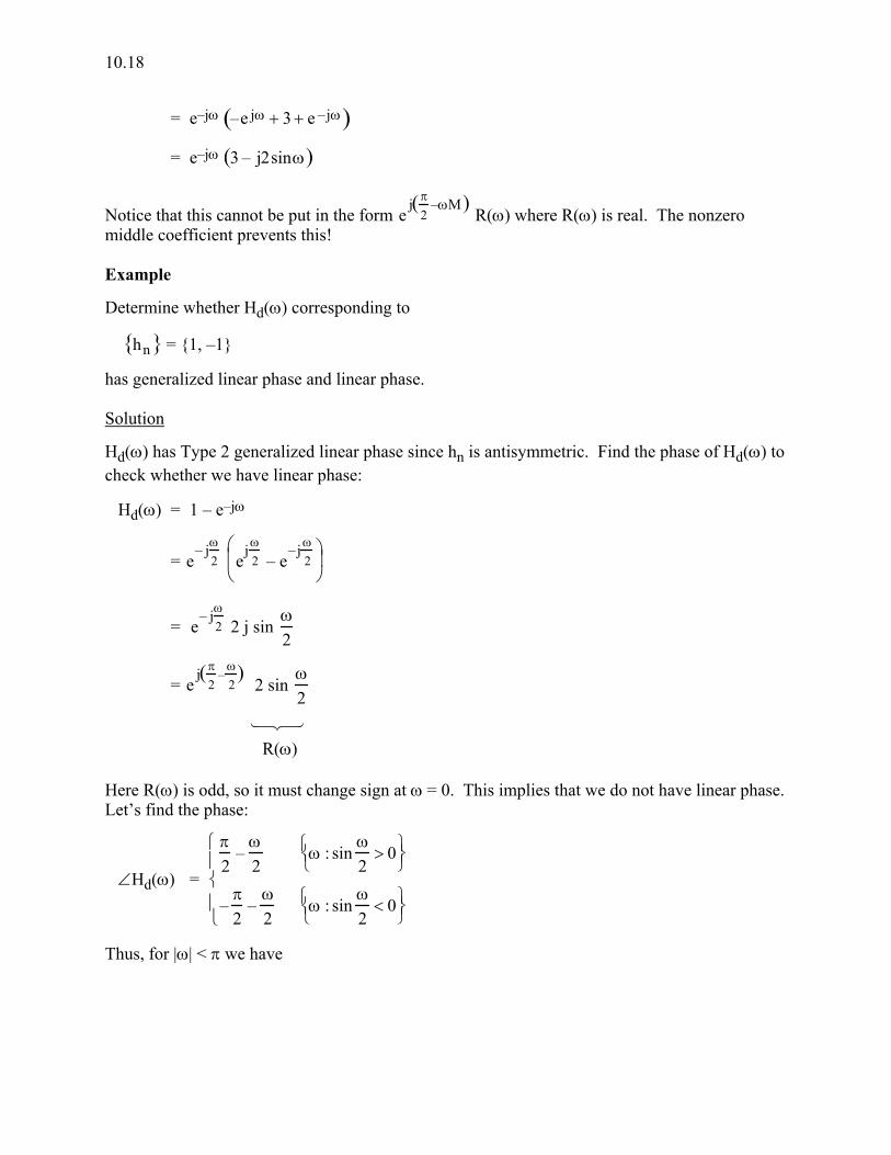
10.18

= e–jω –e jω + 3 + e –jω( )

= e–jω 3 – j2sinω( )

Notice that this cannot be put in the form ej(π

2–ωM)

R(ω) where R(ω) is real. The nonzero middle coefficient prevents this! Example Determine whether Hd(ω) corresponding to hn{ } = {1, –1} has generalized linear phase and linear phase. Solution Hd(ω) has Type 2 generalized linear phase since hn is antisymmetric. Find the phase of Hd(ω) to check whether we have linear phase: Hd(ω) = 1 – e–jω

= e– jω

2 ej ω

2 – e–j ω

2

= e– jω

2 2 j sin

ω2

= ej(π

2–

ω2) 2 sin

ω2

R(ω) Here R(ω) is odd, so it must change sign at ω = 0. This implies that we do not have linear phase. Let’s find the phase:

∠Hd(ω) =

π2

–ω2

ω : sinω2

> 0

–π2

–ω2

ω : sinω2

< 0

Thus, for |ω| < π we have

10.19

∠Hd(ω) =

π2

–ω2

0 < ω < π

–π2

–ω2

–π < ω < 0

This is clearly not linear, as shown in the following plot.

π

−π

−π πω

∠ Hd(ω)

Since R(ω) will be odd for any antisymmetric filter, we conclude that filters with antisymmetric coefficients cannot have linear phase. Example Given hn = {1, 1} ↑ does Hd(ω) have generalized linear phase? How about linear phase? Solution Because of coefficient symmetry, Hd(ω) has Type 1 generalized linear phase. To check linear phase, look at: Hd(ω) = 1 + e–jω

= e– jω

2 ej ω

2 + e– jω

2

= e– jω

2 2cosω2

R(ω) Here R(ω) does not change sign on –π < ω < π and we have

10.20

∠Hd(ω) = – ω2

|ω| ≤ π

⇒ Strictly linear phase. Of course, ∠Hd(ω) is periodic outside |ω| < π. We have:

Hd(ω) = 2 cos ω2

|ω| ≤ π

∠Hd(ω) = – ω2

|ω| ≤ π

So:

−2π 2πω

2

−π π

|Hd(ω)|

π

−2π 2πω

π2

−π2

−π

−π π

∠ Hd(ω)

Here we do have jumps of π at ω = odd multiples of π, but we will still call this linear phase.

10.21

Impact of Coefficient Symmetry on Realizable Frequency Responses Depending on whether hn{ }n=0

N–1 are symmetric or antisymmetric, and N is even or odd, there can

be restrictions on the types of filters that can be realized. Example If N is even (number of coefficients is even) and hn{ }n=0

N–1 are symmetric, then you can’t realize

a high-pass filter! Why not? Because, for this case Hd(π) = 0, so that ω = π can’t be in the passband for this type of filter. Let’s show this. For N even and hn symmetric, we have H(z) = h0 + h1 z–1 + h2 z–2 + … + h2 z–(N–3) + h1 z–(N–2) + h0 z–(N–1) . Then Hd(π) = H(–1) = h0 – h1 + h2 – … – h2 + h1 – h0 = 0 In practice, it pays to be aware of these types of constraints, but the problem is easily resolved. For example, in designing a high-pass filter with symmetric coefficients, we would simply take N to be odd. Let’s now address this problem in more generality by considering some short FIR filters to see what restrictions exist on Hd(0) and Hd(π) as a function of coefficient symmetry and the value of N. Hd(ω) = a0 + a1 e–jω + a1 e–j2ω + a0 e–j3ω (even symmetry, N even)

⇒ Hd (0) = 2a0 + 2a1

Hd (π) = 0

Hd(ω) = a0 + a1 e–jω + a2 e–j2ω + a1 e–j3ω + a0 e–j4ω (even symmetry, N odd)

⇒ Hd(0) = 2a0 + 2a1 + a2

Hd (π) = 2a0 – 2 a1 + a2

Hd(ω) = a0 + a1 e–jω – a1 e–j2ω – a0 e–j3ω (odd symmetry, N even)

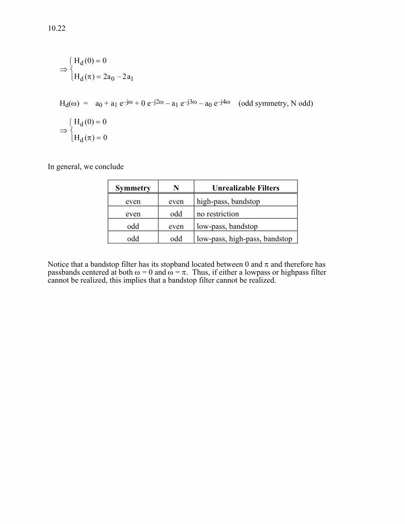
10.22

⇒ Hd (0) = 0

Hd (π) = 2a0 – 2a1

Hd(ω) = a0 + a1 e–jω + 0 e–j2ω – a1 e–j3ω – a0 e–j4ω (odd symmetry, N odd)

⇒ Hd (0) = 0

Hd (π) = 0

In general, we conclude

Symmetry N Unrealizable Filters

even even high-pass, bandstop even odd no restriction odd even low-pass, bandstop odd odd low-pass, high-pass, bandstop

Notice that a bandstop filter has its stopband located between 0 and π and therefore has passbands centered at both ω = 0 and ω = π. Thus, if either a lowpass or highpass filter cannot be realized, this implies that a bandstop filter cannot be realized.