Embed Size (px)
Citation preview
Weather Risk and Cropping Intensity: A Non-Stationary and Dynamic Panel Modeling Approach
Aditya R. Khanal1, Ashok K. Mishra1, and Madhusudan Bhattarai2
1Department of Agricultural Economics and Agribusiness
Louisiana State University, Baton Rouge, LA
2International Crops Research Institute for the Semi-Arid-Tropics (ICRISAT) Patancheru, Hyderabad, India
Contact:
[email protected] (Khanal);
[email protected] (Mishra);
[email protected] (Bhattarai)
Selected Paper prepared for presentation at the Agricultural & Applied Economics Association’s 2014 AAEA Annual Meeting, Minneapolis, MN, July 27-29, 2014.
Copyright 2014 by Khanal, Mishra, and Bhattarai, All rights reserved. Readers may make verbatim copies of this document for non-commercial purposes by any means, provided that this
copyright notice appears on all such copies.

1
Weather Risk and Cropping Intensity: A Non-Stationary and Dynamic Panel Modeling Approach
Aditya R. Khanal, Ashok K. Mishra, and Madhusudan Bhattarai
Abstract
Climatic conditions and weather play an important role in production agriculture. Using district
level panels for 42 years from India and dynamic panel estimation procedure we estimate the
impact of weather risk on cropping intensity. Our non-stationary and dynamic panel model
results suggest that the impact of weather risk on cropping intensity, in rural India, is negative
on short run, while it is positive on long run. Additionally, we found a negative effect of
education on cropping intensity. Finally, in the long run, our results indicate positive effects of
high yielding variety production and share of irrigated land on cropping intensity.
Introduction
Climatic variation influences agricultural production and hence it affects crop
productivity and land use pattern. With population growth and increased challenges for food
security, there has been increased human encroachment on uncultivated fallow and forestlands
and shifting agriculture in developing countries—where majority of the population resides.
Weather risk (also referred to weather variability) not only impacts human settlement but also
puts a greater pressure on agricultural lands and agricultural production. Variability in weather
may lead to variability in agricultural output and subsistence farming in developing countries in
particular, as many rural households cultivate smaller holdings and mostly engage in farming to
raise crops for households’ income and food consumption.
Farmers in developing countries are classified as risk-averse agents (Rosenzweig and
Binswanger 1992; Lamb 2002). In the absence of insurance and credit markets, farmers
undertake ex-ante or ex-post activities to self-insure or to smoothen consumption. There is a
2
growing consensus among policymakers and scientists that weather variability influences the
performance of agriculture and farmers need to adopt strategies to minimize their losses
(Whinston et al., 1981; Rosenzweig and Perry 1994; Seo and Mendelson 2008; Taraz 2012).
This is particularly true for rural farmers in developing countries where agricultural production is
highly dependent on rainfall and sensitive to weather and adaptive capacities are low.
Similarly, farmer’s behavior is affected by weather outcome and affecting cropping
decisions. Farmers in most of the semi-arid regions solely rely on rainfall as a source of
irrigation or moisture for crops; annual and seasonal rainfall patterns influence food crop choice
among farmers in developing countries (Bezabih, Falco, and Yesuf, 2011; Bezabih and Falco
2012). For example, subject to the expectation of high or low rainfall, farmers may alter types of
crops or the area under cultivation. One prospect of weather risk or rainfall variability could be
that it pushes farmers away from farming, inducing occupational shifts or migration to other
areas. However, having fewer opportunities for other alternative income generating opportunities
in the area, as may be the case in most of the rural villages, it is plausible that variability in
rainfall induces farmers to allocate even more land area for different crop portfolio with the
objective of loss minimization. In other words, subject to a higher variation in rainfall, farmers
may diversify crops by bringing in more area under different crops such that the income risk is
minimized by overall returns from non-sensitive crops while compensating for losses in sensitive
crops.
Land use, climatic variability and changes in agricultural productivity have been studied
widely in developing countries (Masvaya, Mupangwa and Twomlow, 2008; Graef and Heigis,
2001). However, literature falls short on assessing the impact of weather risk on cropping
intensity. Additionally, the literature has failed to account for the spatial or temporal nature of
3
risk. It should be of paramount importance that both spatial and temporal phenomena (for
example: climate changes over time, population growth, rural literacy, irrigation availability,
availability of improved varieties etc.) to analyze weather risk in the short and long run.
Utilization of the information in terms of both cross-sectional variation and time variation leads
to better insights; panel data modeling approaches offer such better inferences. Moreover,
policymakers may be interested in methods that mitigate farmer’s sensitivities towards reduction
in weather risk, assessing the impact of climate change, stabilization of food supply, and to
enhance agricultural production and income of farm families under weather adversities.
Therefore, the objective of this study is to assess the impact of weather risk1 on cropping
intensity. We use different class of non-stationary and panel data modeling techniques to
examine the short-term and long-term relationships between weather risk and cropping intensity.
To examine this relationship, we use district-level data compiled by the International Crops
Research Institute for the Semi-Arid-Tropics (ICRISAT2) based on agricultural production and
climatic information, 1966-2007, in rural villages of India.
This paper contributes to the literature in several ways. First, the study uses data that is
long (1966-2007) and has several significant changes in production agriculture, policies, and
weather. Our short- and long- term analysis enables researchers to infer about the impact of
weather risk on cropping intensity in short- and long- runs. For example, inferences from
1Weather risk in this study is measured by variability in rainfall, a major source of weather risk. 2The International Crops Research Institute for the Semi-Arid-Tropics (ICRISAT) is a non-profit agricultural research organization headquartered in Patancheru (Hyderabad, Andhra Pradesh, India) with several regional centers (Niamey (Niger), Nairobi (Kenya)) and research stations Bamako (Mali), Bulawayo (Zimbabwe). It was founded in 1972 by a consortium of organizations convened by the Ford and the Rockefeller Foundations. Its charter was signed by the FAO and the UNDP.
4
short-run analysis may serve as a base for further studies in food crop-portfolio choices, and
income management by farming households not only in developing countries but also in
developed countries. Inferences from long-run behavior contribute to the literature by adding
further insights in farmers’ adaptation to mitigate climate change, an issue that gets wide
attention in recent literature (Rosenberg and Perry 1994; Mendelsohn and Dinar 1999; Macous,
Premand and Vakis, 2012). Second, the paper embraces a comprehensive procedure in empirical
analysis by applying static and dynamic panel data models. The paper proceeds as follows.
Section 2 presents a review of literature related to climate, weather, and rainfall variability in
relation to agriculture and also discusses review of methodological perspectives. Section 3
discusses about data and methodology. Section 4 provides results and discussion. Section 5
concludes.
2. Literature Review
A wide variety of literature in crop sciences and agronomy, development economics, and
agricultural economics have discussed the issue of weather and climatic conditions and it impact
on production agriculture (for example, Rosenzweig and Parry 1994; Seo and Mendelsohn 2008;
Taraz 2012; Bezabih and Falco 2012; Traore et al. 2013; Graef and Haigis 2001). For example,
Traore et al. (2013) investigated the effect of climate and weather on production of cotton,
soybean and groundnut using long-term experimental data from 1965-2005 in Southern Mali.
They found a negative effect of maximum temperature and total seasonal rainfall in cotton yield,
while corn yield was positively correlated with rainfall in relatively drier locations. In another
agronomic study Graef and Haigis (2001) found that the rainfall variability resulted in yield loss
for millet in semi-arid areas in Niger. They reported two major strategies at the farm level that
farmers practice—firstly, cultivate fields in different locations within the village district and
5
secondly, sow as much as area as possible. Both of these strategies result in increased cultivated
area over total cultivable area—in other words, higher cropping intensity or higher land use
intensity for crops.
Form a global perspective, Rosenzweig and Parry (1994) sought to understand the
potential impact of climate change on world food supply. They conclude that vulnerability to
changes in weather and climate is different between developed and developing countries. They
suggest an interdisciplinary research on biophysical and socio-economic aspects to explore the
sensitivity and mitigation towards climate change. Additionally, weather and climatic factors
influence crop choices. For example, Lamb (2002) investigated the impact of weather risk on
crop choices in some of the villages in India and found that crop choices were indeed influenced
by weather risks3. It should be pointed out that land allocation across different crops is an
important decision under weather risk because crops differ widely in terms of yield variability
arising from fluctuation in weather (Lamb 2002).
Recall that variability in rainfall is an important source of uncertainty in agricultural
production decisions. Bezabie, Falco, and Yesuf (2011) used household and plot-specific
longitudinal data from Ethiopia to analyze riskiness of crops and household’s decision on crop
choices. They found that level of riskiness of crop portfolios are partly motivated by both annual
and seasonal rainfall variability and moisture sensitive crops. Household behavior suggested that
they chose less moisture-sensitive crops in times of rainfall shortages and combine risky and
less-risky crops in case of greater variability in rainfall. Therefore, once can conclude that in
response to rainfall variability, farmers are more likely to select less risky crops with less return;
crop selection and crop management practices are ex-ante practices towards mitigating rainfall
3 Weather risk in measured by variability in the start date of monsoon season, with at least 20 mm of rainfall, after June 1st.

6
risk (Bezabih, Falco, and Yesuf, 2011; Bezabih and Falco, 2012). Finally, Seo and Mendelsohn
(2008) investigated South American farmers’ adaptation to climate change. Analyzing the crop
choice among seven most popular crops under different environmental conditions across the
landscape, they concluded that the farmers adjust crop choice and hence area under those crops
to fit their local climate conditions. They also indicated a possibility of crop switching. However,
cross-sectional data did not capture switching over time.
While crop choices, crop mix, production diversifications are ex-ante risk management;
income diversification through off-farm labor supply is explained as major ex-post adjustment.
These studies relate crop production and weather risk with household specific behavior, human
capital, and household’s economic conditions. For example, Dercon (1996, 2000) examined poor
households’ use of risk‐management and risk‐coping strategies and crop choices in Tanzania.
Choosing a less risky crop portfolio, mostly likely behavior of poor households, leads to
substantial low income—resulting from low returns form the crop portfolio. Even with low
returns, households choose low risk crops because they are not able to find jobs in nonfarm
sectors (Dercon, 1996).
Broadly, the major investigations in these studies and a common literature on climatic
conditions and production agriculture can be explained under three major aspects. First, crop
production and yield are affected by weather conditions; second, weather and climatic factors
influence crop choice in general; third, farmers tend to adjust/adapt towards weather risk through
management practices in production (such as crop portfolio choice) or through ex-post income
diversification activities. While adapting towards risk, factors shaping farmers’ behavior such as
household economic conditions, human capital etc. also play an important role.

7
Though the aspects of weather risk, climate change, agricultural production and
adaptation has been discussed in variety of disciplines, concrete evidences based on responses
through farming behavior requires careful attention. However, most of the studies mentioned
above use cross-sectional or aggregate level data. Note that cross-sectional studies and/or
aggregate level time-series studies focused on specific regions may lack generalization. Solid
evidences to back-up theory or strong empirical study to provide a different perspective on
weather risk, crop choice, and cropping intensity is lacking in the literature. Secondly, above
studies have not investigated cropping intensity (cropped area/total cultivable area). Third, to
better understand about farmer’s adjustment behavior in response to weather risk, it is important
to consider short- medium- and long- term effects of weather risk on cropping intensity. Thus,
the literature falls short of concrete empirical evidences that can be generalized. Moreover, due
to possibilities of multi-dimensional factors such as agricultural system, behavioral responses,
and constraints due to weather and other dimensions of risk, the adjustments to weather risk is
more an empirical question that requires careful attention. Our study aims to fill this gap in
empirical literature by providing an evidence of short- and long-run responses to weather risk
and farmer’s behavior using a panel data set, that account for temporal and spatial aspects, from
1966-2007, in 115 district in India.
Conceptual Model
We consider a model of land allocation for cropping decision (acreage decision) of a farm
household. Consider a simple income-leisure utility function of a farm household. The farm
household maximizes the utility function subject to production and time constraints, where utility
is a function of farming household’s income (𝜋) and leisure (𝑙).
𝑈 = 𝑈(𝜋 𝐹,𝑂 𝑒 , 𝑙) (1)
8
We simplify the model with only two potential sources of income, farm income (F)
and/or the income from off-farm jobs (O). We further assume that education is the major
determinant of off-farm earning decisions, O= O(e) and 𝜕𝑂(.)𝜕𝑒
> 0; i.e., farm households with
more educated members in the households are more likely to chose off-farm works in rural areas
over farming. Farm household’s profit function from agriculture is considered as:
𝐹 = 𝑃 ∗ 𝑄 𝐴, 𝐿! ,𝐾,𝜙 − 𝐶(𝑄, 𝑟) (2)
where C(.) represents cost function and Q(.) represent concave production function of a farm
household. P is price of farm output and r is the vector of input prices. Labor and capital inputs
for production are represented as 𝐿!, and K, respectively. 𝐿! is allocated on the basis of total
time by: 𝑇 = 𝐿! + 𝐿! + 𝑙, where T represents total time, 𝐿! is labor provided for farm
production, 𝐿! and l represent off-farm labor supply from household and leisure, respectively.
Land acreage allocation for the agricultural production is represented by 𝐴, with possibility of
acreage allocations for 𝑖 = 1, 2,… . 𝑗 crops such that 𝐴 = 𝐴!! . 𝜙 represents the vector of
other exogenous variables influencing production. For fixed capital and labor inputs (usually in
short-run), land allocation is a major input for total crop production. However, in long run there
could be adjustment in factors.
Now we introduce weather variability and some exogenous factors that influence total
land allocation decisions for crops. Assuming that the total cultivable (total available land for
use) as G, a measure 𝑆! =! (!!)!
, represents the cropping intensity or share of cropped area (total
cropped area over total cultivable area). Let 𝐶! represent weather risk or variability in weather.
Now we represent the weather risk augmented model in equation 3:
𝐹 = 𝑃 ∗ 𝑄 𝑆! 𝐶! , 𝐿! 𝐶! ,𝐾,𝜙 − 𝐶(𝑄, 𝑟) (3)
9
Cropping intensity decisions can represent two scenarios of farmer behavior. First, more
intensity of cropping, i.e., allocate more total acreage under crop as a response towards weather
variability—diversifying the crop portfolio towards response of risk perhaps including more
acreages under less risky crops. 𝜕(𝑆𝐴 𝐶𝑣 )𝜕𝐶𝑣
> 0 implies such behavior. Second, lower intensity of
cropping, i.e., allocate less acreage under agricultural crops when weather variability is
increased. 𝜕(𝑆𝐴 𝐶𝑣 )𝜕𝐶𝑣
< 0 may imply that the farmer moves away from cropping. In the nutshell,
we can assume that the households with potential higher off-farm opportunities may move away
from farming when weather variability is higher—perhaps households with more educated
members, i.e., we expect 𝜕!! !!𝜕!!
< 0 in equation 3 and 𝜕!(!)𝜕!!
> 0 in utility function in equation
1.
Econometric Method
Equation 3 can be transformed to derive the empirical model. Empirically, we estimate
the short-term and long-term sensitivity of cropping intensity to rainfall variability as follows.
𝑆!!,! = Γ𝐶!!,! + 𝛽𝑋!" + 𝛼! + 𝜀!" (4)
𝑆!!,! represents cropping intensity in the district i in year t. Our main variable of interest, rainfall
variability in district i in year t is represented as 𝐶!!,!. 𝑋!" includes exogenous control variables
that may affect cropping intensity, such as share of rural literates in the district, share of
cultivators in total population, productivity of high yielding variety, availability of agricultural
labor, net irrigated area over total cultivable area etc. 𝛼! is useful in controlling district-level
fixed effects.
In our study, equation 4 is estimated using panel data. Broadly, two types of panel data
models have been discussed in literature—firstly, the models with large cross-sectional units but
10
small time-span (large N, smaller (or fixed) T), and secondly, models with larger time span as
well as larger cross-sectional units (larger N, larger T). The former types of panel model require
pooling individual groups and allowing only the intercepts to differ across the groups. On this
extreme, we can estimate the fixed effects model in which the time series data for each group are
pooled and only the intercepts are allowed to differ across the groups4. However, if the slope
coefficients are not identical, these estimators could result in misleading inferences. Previous
studies have found that the assumption of homogeneity of parameters across group is often
inappropriate (Phillips and Moon, 2000; Baltagi 2005; Pesaran, Shin, and Smith, 1999).
In recent years, there has been a growing interest in cases, such as sets of countries,
regions or industries, where there are fairly long time-series for a large N. The second approach
can be utilized in estimation of non-stationary or co-integrated panel models where heterogeneity
in parameters is allowed across groups. Econometric methods for non-stationary panels are
applied in many empirical studies. Some recent studies, for example, include—Narayan et al.
(2010); Mark and Sul (2003); Costantini and Martini (2009); Onel (2012).
Persaran, Shin, and Smith (1997, 1999) present techniques to estimate non-stationary
dynamic panels in which the parameters are heterogeneous across groups—the mean-group
(MG) and pooled mean group (PMG) estimators. With MG estimator, the intercepts, slope
coefficients, and error variances are all allowed to differ across groups. The PMG estimator, on
the other hand, combines both pooling and averaging. This allows the intercept, short run
coefficients, and error variances to differ across the groups but constraints the long run
coefficients to be equal across group. Pesaran, Shin, and Smith (1999) have developed maximum
likelihood methods to estimate these parameters (Blackburne III and Frank, 2007).
4For detail description of panel data models, we refer to Baltagi (2005).
11
Bangake and Eggo (2010) estimated long run relationships using MG, PMG, and
dynamic OLS models to study international capital mobility in African countries using 37
African countries from 1970 to 2006. Frank (2005) used MG and PMG models to study income
inequality and economic growth relations in the long-term.
In this paper, we presented the results of both classes of panel data models (first, models
for fixed T and large N and second, models for large T and large N). Assuming fixed T and large
N, we presented results of static fixed effect (FE) models, static random effect (RE) models, and
first difference (FD) models. For the second-class or co-integrated models, we presented
regressions applying dynamic OLS (DOLS) regression, dynamic fixed effects (DFE) regression,
and MG and PMG model estimations. MG and PMG models (Persaran, Shin, and Smith (1997,
1999)) are estimated to assess the long run and short run effects of rainfall variability in cropping
intensity.
Data
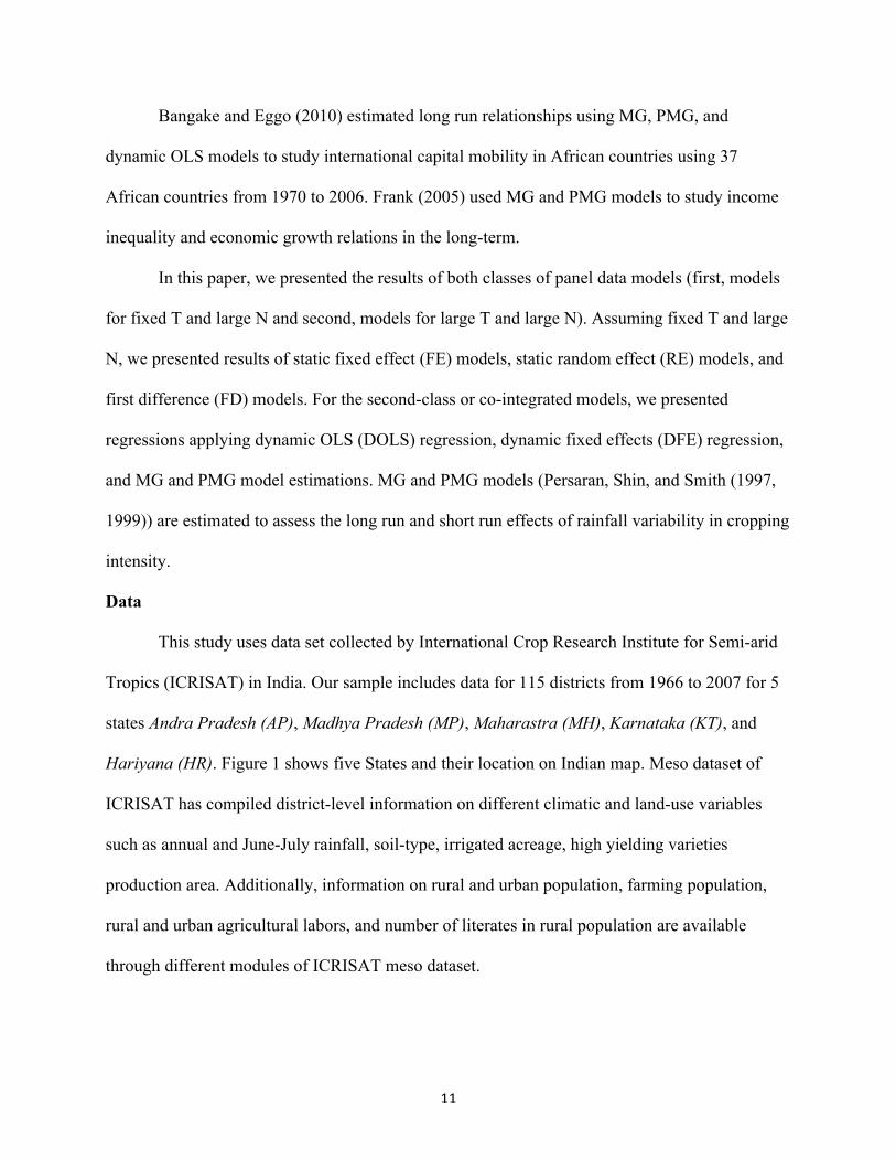
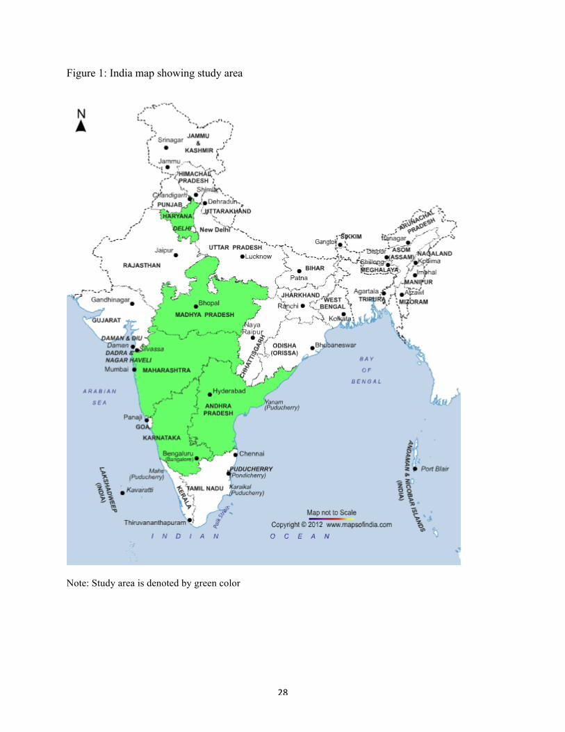
This study uses data set collected by International Crop Research Institute for Semi-arid
Tropics (ICRISAT) in India. Our sample includes data for 115 districts from 1966 to 2007 for 5
states Andra Pradesh (AP), Madhya Pradesh (MP), Maharastra (MH), Karnataka (KT), and
Hariyana (HR). Figure 1 shows five States and their location on Indian map. Meso dataset of
ICRISAT has compiled district-level information on different climatic and land-use variables
such as annual and June-July rainfall, soil-type, irrigated acreage, high yielding varieties
production area. Additionally, information on rural and urban population, farming population,
rural and urban agricultural labors, and number of literates in rural population are available
through different modules of ICRISAT meso dataset.

12
Table 1 presents variable definitions and summary statistics in raw form (i.e, summary of
district-time data points). In total we have 4,782 district and time observations were used in our
analysis. We calculated district-level cropping intensity as the ratio of total cropped area to total
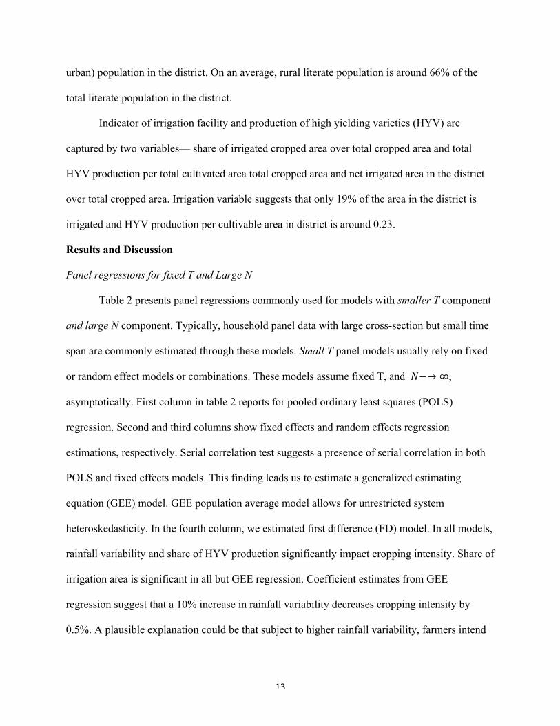
available area for cultivation (excluding area for non-agricultural uses, buildings, etc.). Average
cropping intensity is 0.627 with standard deviations of 0.267. This indicates that around 63% of
the total cultivable area has been allocated for agricultural production of the crops in a district.
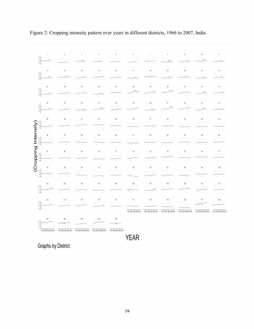
The cropping intensity pattern for each district is represented in figure 2. Overall, figures suggest
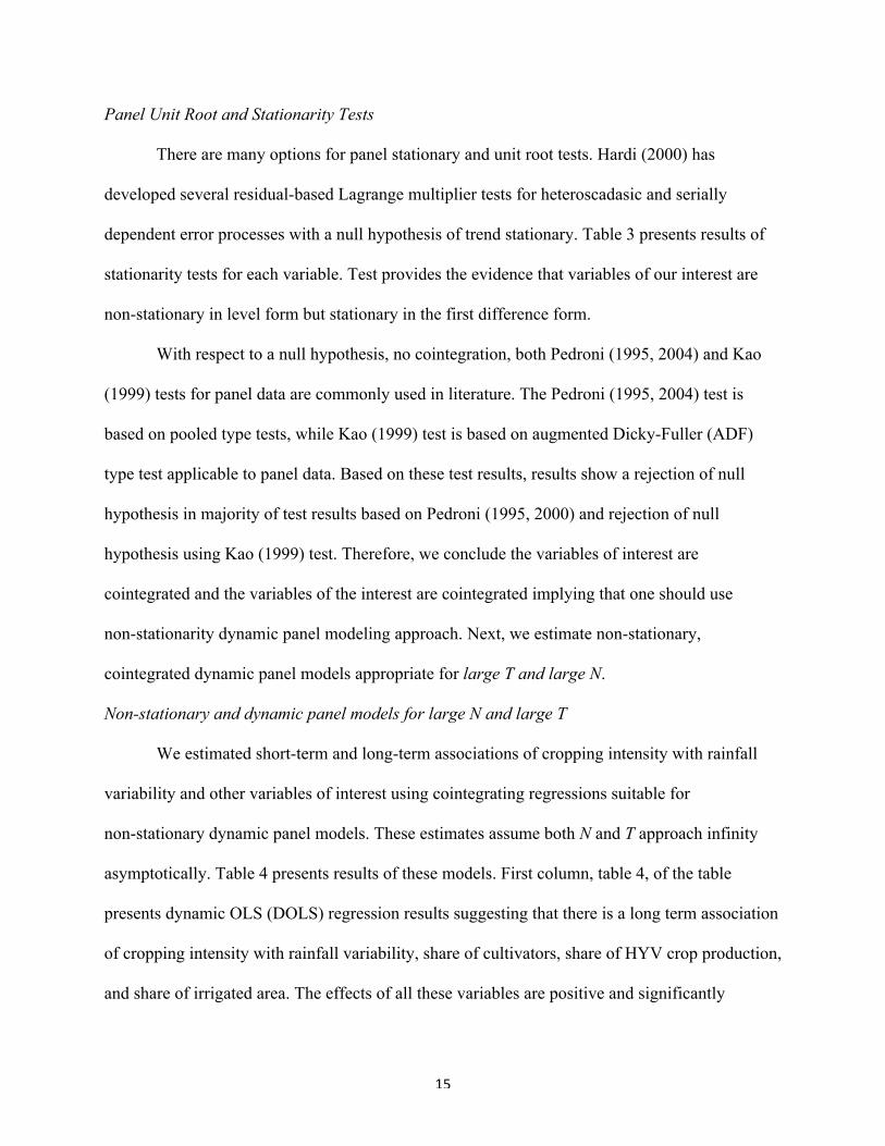
a slightly increasing trend in most of the districts over time. Rainfall variability, indicator of
weather risk is measured by the coefficient of variation of the annual rainfall. Coefficient of
variation is a unit-less measure and has been used in other studies as a measure of variability or
risk (see, Mishra and Goodwin 1997; Bezabih et al., 2011). Average rainfall variability was 0.537
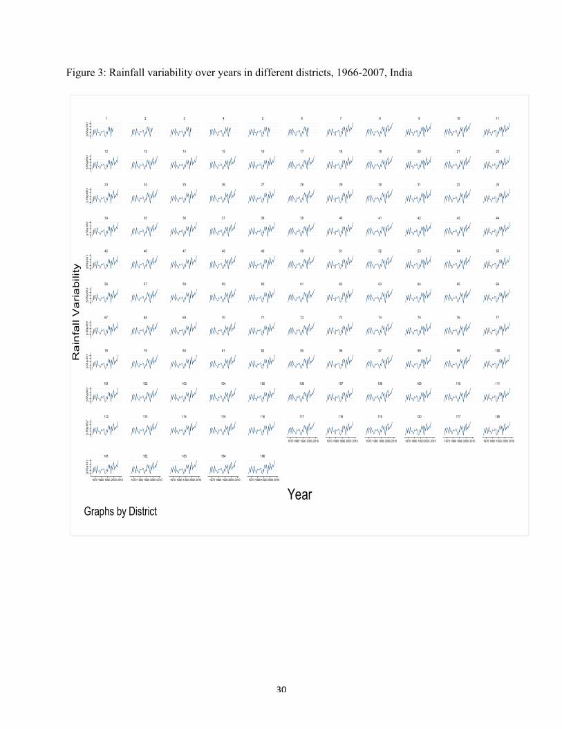
with standard deviation of 0.051. Rainfall variability is measured on a yearly basis. Figure 3
represents rainfall variability plots in each district and over time.
Cultivator share is the share of total cultivators (farmers) in total district population. In
another perspective, this measure indicates the number of many famers that are available to
cultivate in the district population. Surprisingly, this is only about 16% compared to the total
district population. Agricultural labor availability is calculated as the ratio of total agricultural
labor available in the district to total cultivators. Labor availability variable with mean of 0.865
indicates that agricultural labor availability per cultivator was around 86%. However, relatively
higher standard deviation of 0.623 indicates that the district-time labor availability has higher
variation across time and space. Another variable of interest is the literacy rate in the rural areas.
Our rural literate share variable is the ratio of rural literate population to total literate (rural and
13
urban) population in the district. On an average, rural literate population is around 66% of the
total literate population in the district.
Indicator of irrigation facility and production of high yielding varieties (HYV) are
captured by two variables— share of irrigated cropped area over total cropped area and total
HYV production per total cultivated area total cropped area and net irrigated area in the district
over total cropped area. Irrigation variable suggests that only 19% of the area in the district is
irrigated and HYV production per cultivable area in district is around 0.23.
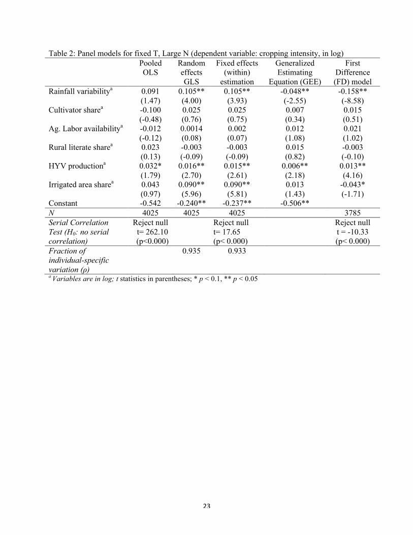
Results and Discussion
Panel regressions for fixed T and Large N
Table 2 presents panel regressions commonly used for models with smaller T component
and large N component. Typically, household panel data with large cross-section but small time
span are commonly estimated through these models. Small T panel models usually rely on fixed
or random effect models or combinations. These models assume fixed T, and 𝑁−→ ∞,
asymptotically. First column in table 2 reports for pooled ordinary least squares (POLS)
regression. Second and third columns show fixed effects and random effects regression
estimations, respectively. Serial correlation test suggests a presence of serial correlation in both
POLS and fixed effects models. This finding leads us to estimate a generalized estimating
equation (GEE) model. GEE population average model allows for unrestricted system
heteroskedasticity. In the fourth column, we estimated first difference (FD) model. In all models,
rainfall variability and share of HYV production significantly impact cropping intensity. Share of
irrigation area is significant in all but GEE regression. Coefficient estimates from GEE
regression suggest that a 10% increase in rainfall variability decreases cropping intensity by
0.5%. A plausible explanation could be that subject to higher rainfall variability, farmers intend

14
to move away from agriculture and perhaps choose to diversify income through other sources,
perhaps with off-farm and non-agricultural works.
Unlike rest of the estimates presented in Table 2, FD regression relates a change (first
difference) in cropping intensity variable with changes (first difference) in independent variables.
Results show that a 1% increase in change in rainfall variability from previous year results a
decrease in change in cropping intensity by 1.6%. Taking results from the GEE and FD models
together, our results show that risk has a negative effect on cropping intensity and is decreasing
over time. The positive effect of share of HYV production on cropping intensity, on the other
hand, is increasing over time. For example, 10% increase in the share of HYV crop, changes
cropping intensity by 0.1%.
However, one must be cautious in infering relationships from our aggregate district level
data using large N and small T panel models presented in Table 2. Large N and small T panel
models require pooling individual groups and allow only the intercepts to differ across groups.
By the nature of our data, we have much longer time span (T) along with substantial
cross-sectional groups. As indicated in previous studies, homogeneity of slope parameters, the
assumption of large N and small T, is often inappropriate for case where we have large T and
large N (Pesaran and Smith 1995; Phillips and Moon 2000; Baltagi 2005). Asymptotic of large T
and large N dynamic panel models is different from traditional large N and small T dynamic
panels (Baltagi, 2005). With increase in time observations inherent in large N and large T
dynamic panels is non-stationarity that needs to be addressed. Therefore one needs to test for
non-stationarity using stationary, unit root, and cointegration tests. Next, we proceed to panel
non-stationary and unit root, and co-integration tests.
15
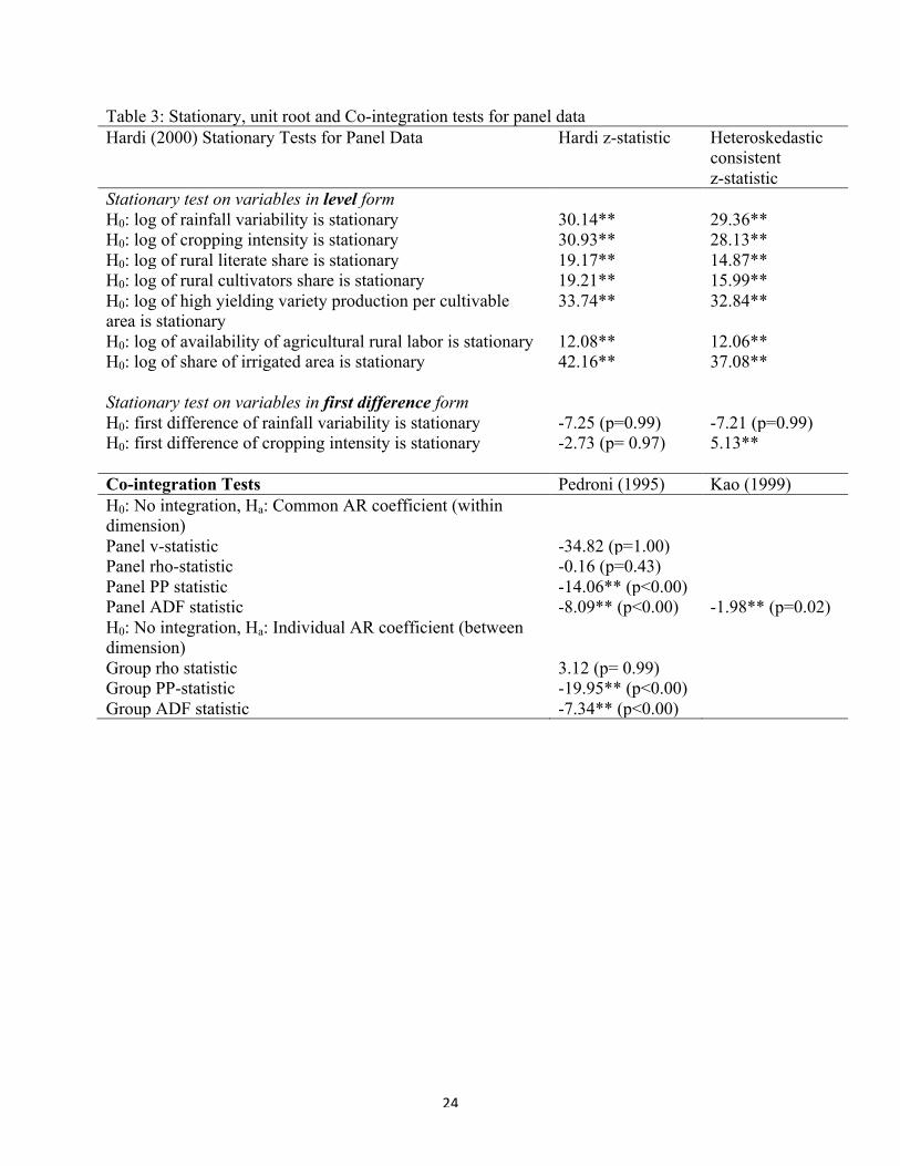
Panel Unit Root and Stationarity Tests
There are many options for panel stationary and unit root tests. Hardi (2000) has
developed several residual-based Lagrange multiplier tests for heteroscadasic and serially
dependent error processes with a null hypothesis of trend stationary. Table 3 presents results of
stationarity tests for each variable. Test provides the evidence that variables of our interest are
non-stationary in level form but stationary in the first difference form.
With respect to a null hypothesis, no cointegration, both Pedroni (1995, 2004) and Kao
(1999) tests for panel data are commonly used in literature. The Pedroni (1995, 2004) test is
based on pooled type tests, while Kao (1999) test is based on augmented Dicky-Fuller (ADF)
type test applicable to panel data. Based on these test results, results show a rejection of null
hypothesis in majority of test results based on Pedroni (1995, 2000) and rejection of null
hypothesis using Kao (1999) test. Therefore, we conclude the variables of interest are
cointegrated and the variables of the interest are cointegrated implying that one should use
non-stationarity dynamic panel modeling approach. Next, we estimate non-stationary,
cointegrated dynamic panel models appropriate for large T and large N.
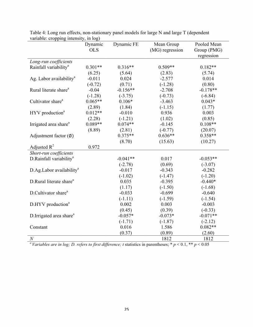
Non-stationary and dynamic panel models for large N and large T
We estimated short-term and long-term associations of cropping intensity with rainfall
variability and other variables of interest using cointegrating regressions suitable for
non-stationary dynamic panel models. These estimates assume both N and T approach infinity
asymptotically. Table 4 presents results of these models. First column, table 4, of the table
presents dynamic OLS (DOLS) regression results suggesting that there is a long term association
of cropping intensity with rainfall variability, share of cultivators, share of HYV crop production,
and share of irrigated area. The effects of all these variables are positive and significantly
16
different from zero at the 5% level of significance or higher. The DOLS has a remarkably high
R-square 0.972 suggesting that the model explains cropping intensity very well in long run.
DOLS results suggest that 10% change in rainfall variability increases cropping intensity by 3%.
The long-term effect of a 10% change in share of cultivator, share of HYV crop production, and
share of irrigated areas increase change in cropping intensity by 0.7%, 0.1%, and 0.9%,
respectively.
Column 2 of table 4 shows the results of dynamic fixed effects (DFE) model. DFE has
similar coefficient estimates as DOLS except that it suggests one additional variable affecting
cropping intensity. Results show that share of rural literates is negatively cropping intensity in
long-term. A 10% increase in change in share of rural literate results in a 1.6% reductions in
cropping intensity in the long-term.
Allowing for the heterogeneity of parameters across groups, Pesaran, Shin, and Smith
(1997, 1999) have developed two important techniques to estimate non-stationary dynamic panel
models: The mean group (MG) and pooled mean group (PMG) estimators. The MG estimator
relies on estimating N-time series regressions and averaging the coefficients, whereas the PMG
estimator relies on a combination of pooling and averaging the coefficients (Pesaran and Smith
1995; Pesaran, Shin, and Smith 1999). These estimation techniques have been applied to
empirical studies (Freeman 2000; Frank 2005). Column 3 and column 4 of our results in table 4
present mean-groups (MG) and poled mean groups (PMG) regression, respectively. MG results
suggest a positive 0.5% growth in cropping intensity as a result of 1% increase in change in
weather variability while PMG estimator suggests a positive effect of around 0.2%. Additionally,
PMG result suggest a negative long term effect of share of rural literates and a positive effect of
17
share of irrigated area on cropping intensity. A 10% growth in share of rural literates is
associated with a 1.8% reduction in change in cropping intensity.
We conducted a Hausman test to compare which model is more suitable among DFE,
MG, and PMG. Test results are presented in table 5. Our two sets of Hausman test suggest that
DFE model is preferred over MG model and PMG model is preferred over MG model. Overall,
DFE and PMG model estimates suggest a positive long-term effect of growth in rainfall
variability, a negative long-term effect of growth in share of rural literates, and a positive effect
of a growth in share of irrigated area. A positive effect of rainfall variability suggests for the
portfolio or crop mix diversification behavior of farmers that we have discussed as one of the
possibilities in our conceptual model—i.e., increase in cropped area (perhaps with higher
allocated areas for less risky crops) when subjected to higher variability in rainfall. This may
seem dubious at first glance because one assumes that there is a more likely chance of moving
away from farming and diversify income through alternative off-farm jobs when farming
becomes riskier—resulting a lower cropping intensity due to weather risk. However, the scenario
of peasant farmers in rural areas may be different from this assumption because they may have
less opportunity for alternative practices and continue farming. A positive relation is plausible.
Farmers with low or no outside opportunities, the response towards weather risk is to crop more
areas in different locations and with different crops (crop mix).
A negative effect of share of rural literate share variable in the district could be explained
through education and off-farm labor supply relations established in farm household literature.
Increased education in rural area increases off-farm work opportunities for the educated; this
may induce farmers to move away from farming and towards off-farm work that is often less
variable and parameters. Increase in share of HYV to total cropped area is an indication of
18
adoption of improved varieties and progressive farming. Higher HYV production pattern
increases cropping intensity as more people are attracted by higher yield in crops and increased
returns and thus aim to expand farming or attracted towards farming. A positive effect of a
growth in share of irrigated area on growth in cropping intensity is as expected. With irrigation
facilities, farmers are better able to reduce the impact of rainfall variability and thus able to
stabilize production and income from farming. This enables existing farmers to expand cropping
areas, increasing economies of scale.
Finally, we also examined the long-term effect of rainfall variability and cropping
intensity using DFE, MG, and PMG estimators in state-wise regression for 3-states. Results are
shown in table 6. A positive effect of rainfall variability is also confirmed in state-wise
regression indicating robustness of our findings.
Summary and Conclusion
Weather and climatic conditions play an important role in agricultural production.
Variability and risks associated with climate and weather in an area not only influence farmer’s
decision on cropping intensity and pattern but may also influence the decision to farm in the first
place. This paper presents empirical evidence on a relationship between cropping intensity and
weather variability using a panel of 115 districts in India over the 1966 to 2007 period. We
presented results using different panel data methods used in the literature. Rather than 115
cross-sections with 5 or 6 time periods, as is common in most of the prior panel data studies, we
are able to compile a sample that is large in both cross-sections and time-periods (N=115, T=42)
and enables us to implement a more suitable non-stationary cointegrated dynamic panel model
for large T and large N.

19
Results indicate a positive long-term association between rainfall variability on cropping
intensity. The positive relation is quite strong and robust among all different panel data
models—dynamic OLS, dynamic FE, mean group, and pooled mean group estimation
techniques. The findings are significant and consistent even with the inclusion of numerous
additional regressors. Additionally, our results suggest that the indicator of higher education in
the district is negatively associated with cropping intensity while indicators of irrigation facilities
and share of high yielding variety production positively influence cropping intensity.
With an opportunity to choose alternative income generating activities such as off-farm
jobs, a positive effect of weather risk on cropping intensity may seem dubious because when
farming is risky, people may move away from farming. However, the scenario of peasant
households in rural areas and subsistence farming could be different in that they have fewer
off-farm alternatives. Instead, in this case a response towards weather risk would be to diversify
crop mix and increase the allocated areas for less risky crops, that will intend to have stabilized
quantity of food produced and income generated. This latter behavior results in increase in
cropping intensity. However, we have not tested for crop specific area allocations in this study
and warrants for further extension. Other limitations of this study may come from a district-level
aggregate data. A micro-level crop-specific data on cropping intensity and pattern will be more
helpful to verify this behavior. Further, land quality and land type variables may also help in
providing better insights.
20
References
Baltagi, Badi. Econometric Analysis of Panel Data. Wiley Publication, 2005. Bangake, Chrysost, and Jude C. Eggoh. 2010. "International Capital Mobility in African
Countries: A Panel Cointegration Analysis." Conference paper, http://www.csae.ox.ac.uk/conferences/2010-EdiA/papers/241-Bangake.pdf
Bezabih, Mintewab, and Salvatore Di Falco. "Rainfall variability and food crop portfolio choice: evidence from Ethiopia." Food Security 4.4 (2012): 557-567.
Bezabih, M., and S. D. Falco and M. Yesuf. Farmer’s Response to Rainfall Variability and Crop Portfolio Choice: Evidence from Ethiopia. Discussion paper, Environment for Development. EFD DP 11-10, (2011). http://www.rff.org/RFF/Documents/EfD-DP-11-10.pdf
Blackburne III, Edward F., and Mark W. Frank. "Estimation of Nonstationary Heterogeneous Panels." Stata Journal 7.2 (2007): 197-208.
Cameron, Adrian Colin, and Pravin K. Trivedi. Microeconometrics Using Stata. Vol. 5. College Station, TX: Stata Press, 2009.
Costantini, Valeria, and Chiara Martini. "The Causality between Energy Consumption and Economic Growth: a Multi-sectoral Analysis Using Non-stationary Cointegrated Panel Data." Energy Economics 32.3 (2010): 591-603.
Dercon, S. “Risk, crop choice, and savings: Evidence from Tanzania.” Economic Development and Cultural Change, 44, 3, (1996): 485-514.
Dercon, S. “Income Risk, Coping Strategies, and Safety Nets.” The World Bank Research Observer, 17, 2, (2002): 141-166.
Graef, F., and J. Haigis. "Spatial and Temporal Rainfall Variability in the Sahel and its Effects on Farmers' Management Strategies." Journal of Arid Environments 48.2 (2001): 221-231.
Hadri, Kaddour. "Testing for Stationarity in Heterogeneous Panel Data." The Econometrics Journal 3.2 (2000): 148-161.
Kao, Chihwa. "Spurious regression and residual-based tests for cointegration in panel data." Journal of econometrics 90.1 (1999): 1-44.
Lamb, R. L. Weather Risk, Crop Mix and Wealth in the Semi-arid Tropics. Department of Agricultural and Resource Economics Report No, 25, 2002.
Macours, K., P. Premand, and R. Vakis, “Transfers, Diversification, and Household Risk Strategies," 2012. Policy Research Working Paper 6053, The World Bank.
Masvaya, E., W. Mupangwa, and S. Twomlow. Rainfall Variability Impacts on Farmers’ Management Strategies and Crop Yields. Paper presented at the 9th Water Net/WARFSA/GWP-SA Annual Symposium, Johannesburg, South Africa, 29-31 October 2008. Amsterdam, Netherlands: WaterNet.
Mendelsohn, Robert, and Ariel Dinar. "Climate change, agriculture, and developing countries: does adaptation matter?." The World Bank Research Observer 14.2 (1999): 277-293.
Mishra, A. K., and B. K. Goodwin. "Farm Income Variability and the Supply of Off-farm Labor." American Journal of Agricultural Economics 79.3 (1997): 880-887.
Narayan, P. K., S. Narayan, A. Prasad, and B.C. Prasad. Tourism and Economic Growth: A Panel Data Analysis for Pacific Island Countries. Tourism economics, 16,1, (2010):169-183.
21
Onel, G. "The Use of Nonstationary Panel Time Series Data in the Analysis of Farmland Values." 2012 Annual Meeting, August 12-14, 2012, Seattle, Washington. No. 124893. Agricultural and Applied Economics Association, 2012.
Pesaran, M. Hashem, and Ron Smith. "Estimating Long-run Relationships from Dynamic Heterogeneous Panels." Journal of Econometrics 68.1 (1995): 79-113.
Pesaran, M. Hashem, Yongcheol Shin, and Ron P. Smith. "Pooled Mean Group Estimation of Dynamic Heterogeneous Panels." Journal of the American Statistical Association 94.446 (1999): 621-634.
Pedroni, Peter. "Critical values for cointegration tests in heterogeneous panels with multiple regressors." Oxford Bulletin of Economics and statistics 61.S1 (1999): 653-670.
Phillips, Peter CB, and Hyungsik R. Moon. "Nonstationary Panel Data Analysis: An Overview of Some Recent Developments." Econometric Reviews 19.3 (2000): 263-286.
Rosenzweig, Mark R. and Hans P. Binswanger, “Wealth, Weather Risk and the Composition and Profitability of Agricultural Investments,” Policy Research Working Paper Series 1055, The World Bank 1992.
Rosenzweig, Cynthia, and Martin L. Parry. "Potential impact of climate change on world food supply." Nature 367.6459 (1994): 133-138.
Seo, S. Niggol, and Robert Mendelsohn. "An analysis of crop choice: Adapting to climate change in South American farms." Ecological Economics 67.1 (2008): 109-116.
Taraz, Vis. “Adaption to Climate Change: Historical Evidence from the Indian Monsoon," 2012. http://www.econ.yale.edu/_vt48/Vis Taraz jmp.pdf.
Traore, B., M. Corbeels, , M. T., van Wijk, M. C. Rufino, and K.E. Giller. “Effects of Climate Variability and Climate Change on Crop Production in Southern Mali.” European Journal of Agronomy, 49, (2013): 115-125.
Whitson, Robert E., et al. “Machinery and crop selection with weather risk.” Transactions of the ASAE [American Society of Agricultural Engineers] 24 (1981).

22
Table 1: Descriptive Statistics of the variables in raw form, 1966 to 2007, India
Variable definition Mean Standard
Deviation
Cropping intensity (Total cropped area over total available cultivable area) 0.627 0.267
Rainfall variability (Coefficient of variation of total annual rainfall) 0.537 0.051
Cultivator share (Share of total cultivators (farmers) in total population) 0.159 0.059
Agricultural labor availability (Total agricultural labor population over total
cultivators population)
0.865 0.623
Rural literate share (Share of rural literate population over total literates) 0.664 0.160
HYV production (High yielding variety production over gross cropped area) 0.228 0.181
Irrigated area share (Net irrigated area over total cropped area) 0.190 0.145
Total observations 4782
23
Table 2: Panel models for fixed T, Large N (dependent variable: cropping intensity, in log) Pooled
OLS Random effects GLS
Fixed effects (within)
estimation
Generalized Estimating
Equation (GEE)
First Difference (FD) model
Rainfall variabilitya 0.091 0.105** 0.105** -0.048** -0.158** (1.47) (4.00) (3.93) (-2.55) (-8.58) Cultivator sharea -0.100 0.025 0.025 0.007 0.015 (-0.48) (0.76) (0.75) (0.34) (0.51) Ag. Labor availabilitya -0.012 0.0014 0.002 0.012 0.021 (-0.12) (0.08) (0.07) (1.08) (1.02) Rural literate sharea 0.023 -0.003 -0.003 0.015 -0.003 (0.13) (-0.09) (-0.09) (0.82) (-0.10) HYV productiona 0.032* 0.016** 0.015** 0.006** 0.013** (1.79) (2.70) (2.61) (2.18) (4.16) Irrigated area sharea 0.043 0.090** 0.090** 0.013 -0.043* (0.97) (5.96) (5.81) (1.43) (-1.71) Constant -0.542 -0.240** -0.237** -0.506** N 4025 4025 4025 3785 Serial Correlation Test (H0: no serial correlation)
Reject null t= 262.10 (p<0.000)
Reject null t= 17.65 (p< 0.000)
Reject null t = -10.33 (p< 0.000)
Fraction of individual-specific variation (ρ)
0.935 0.933
a Variables are in log; t statistics in parentheses; * p < 0.1, ** p < 0.05
24
Table 3: Stationary, unit root and Co-integration tests for panel data Hardi (2000) Stationary Tests for Panel Data Hardi z-statistic Heteroskedastic
consistent z-statistic
Stationary test on variables in level form H0: log of rainfall variability is stationary 30.14** 29.36** H0: log of cropping intensity is stationary 30.93** 28.13** H0: log of rural literate share is stationary 19.17** 14.87** H0: log of rural cultivators share is stationary 19.21** 15.99** H0: log of high yielding variety production per cultivable area is stationary
33.74** 32.84**
H0: log of availability of agricultural rural labor is stationary 12.08** 12.06** H0: log of share of irrigated area is stationary 42.16** 37.08**
Stationary test on variables in first difference form H0: first difference of rainfall variability is stationary -7.25 (p=0.99) -7.21 (p=0.99) H0: first difference of cropping intensity is stationary -2.73 (p= 0.97) 5.13** Co-integration Tests Pedroni (1995) Kao (1999) H0: No integration, Ha: Common AR coefficient (within dimension)
Panel v-statistic -34.82 (p=1.00) Panel rho-statistic -0.16 (p=0.43) Panel PP statistic -14.06** (p<0.00) Panel ADF statistic -8.09** (p<0.00) -1.98** (p=0.02) H0: No integration, Ha: Individual AR coefficient (between dimension)
Group rho statistic 3.12 (p= 0.99) Group PP-statistic -19.95** (p<0.00) Group ADF statistic -7.34** (p<0.00)
25
Table 4: Long run effects, non-stationary panel models for large N and large T (dependent variable: cropping intensity, in log) Dynamic
OLS Dynamic FE Mean Group
(MG) regression Pooled Mean Group (PMG)
regression Long-run coefficients Rainfall variabilitya 0.301** 0.316** 0.509** 0.182** (6.25) (5.64) (2.83) (5.74) Ag. Labor availabilitya -0.011 0.024 -2.577 0.014 (-0.72) (0.71) (-1.28) (0.80) Rural literate sharea -0.04 -0.156** -2.708 -0.178** (-1.28) (-3.75) (-0.73) (-6.84) Cultivator sharea 0.065** 0.106* -3.463 0.043* (2.89) (1.84) (-1.15) (1.77) HYV productiona 0.012** -0.010 0.936 0.003 (2.28) (-1.21) (1.02) (0.85) Irrigated area sharea 0.089** 0.074** -0.145 0.108** (8.89) (2.81) (-0.77) (20.07) Adjustment factor (∅) 0.375** 0.636** 0.358** (8.70) (15.63) (10.27) Adjusted R2 0.972 Short-run coefficients D.Rainfall variabilitya -0.041** 0.017 -0.053** (-2.78) (0.69) (-3.07) D.Ag.Labor availabilitya -0.017 -0.343 -0.282 (-1.02) (-1.47) (-1.20) D.Rural literate sharea 0.035 -0.395 -0.440* (1.17) (-1.50) (-1.68) D.Cultivator sharea -0.033 -0.699 -0.640 (-1.11) (-1.59) (-1.54) D.HYV productiona 0.002 0.003 -0.003 (0.45) (0.39) (-0.33) D.Irrigated area sharea -0.057* -0.073* -0.071** (-1.71) (-1.87) (-2.12) Constant 0.016 1.586 0.082** (0.37) (0.89) (2.60) N 1812 1812 a Variables are in log; D. refers to first difference; t statistics in parentheses; * p < 0.1, ** p < 0.05

26
Table 5: Hausman test results for model choice between FE, MG, PMG models Hausman test Hypothesis Chi-square
Statistics Conclusion
Comparison between MG and Dynamic FE
MG estimator is consistent under null and alternative FE is inconsistent under alternative, efficient under null
2.59 (p >chi2 = 0.86)
FE model, efficient under null, is preferred over MG model
Comparison between MG and PMG regression
MG estimator is consistent under null and alternative PMG estimator is inconsistent under alternative, efficient under null
0.00 (p > chi2 = 1.00)
PMG estimator, the efficient estimator under the null hypothesis, is preferred

27
Table 6: Long run effects using non-stationary panel models, state-wise regressions Dynamic FE Mean Group (MG) Pooled Mean Group (PMG) State: Andra Pradesh (AP) Rainfall variabilitya 0.388** 1.045** 0.289** (4.47) (2.48) (3.94) Ag. Labor availabilitya 0.043 -1.370 0.025 (0.48) (-0.65) (0.46) Rural literate sharea -0.130** 1.390 -0.083 (-2.02) (1.29) (-1.37) Cultivator sharea 0.172* -1.144 0.178** (1.70) (-0.39) (2.46) HYV productiona -0.006 -0.011 0.018** (-0.51) (-1.01) (2.78) Irrigated area sharea -0.125** -0.032 -0.128** (-2.58) (-0.23) (-5.70) Adjustment factor (∅) 0.402** 0.712** 0.397** (8.03) (11.17) (7.65) N 658 658 State: Hariyana (HP) Rainfall variabilitya 0.314** 0.234** 0.288** (2.78) (2.86) (3.03) Ag. Labor availabilitya 0.134 -13.49 -0.019 (1.46) (-1.00) (-0.38) Rural literate sharea -0.002 -25.80 -0.045 (-0.01) (-0.94) (-0.54) Cultivator sharea 0.0742 -20.54 -0.108** (1.22) (-0.99) (-2.16) HYV productiona 0.124* 6.856 0.028 (1.85) (1.01) (0.92) Irrigated area sharea -0.020 -1.364 0.087** (-0.46) (-1.04) (2.28) Adjustment factor (∅) 0.463** 0.622** 0.293** (3.72) (4.85) (2.12) N 259 259 State: Maharastra (MH) Rainfall variabilitya 0.271** 0.158 0.140** (2.92) (1.32) (4.17) Ag. Labor availabilitya 0.035 -0.488 0.021 (0.77) (-0.71) (0.98) Rural literate sharea -0.272** 0.479 -0.237** (-3.89) (0.52) (-6.68) Cultivator sharea 0.163** -0.538 0.068** (2.38) (-0.57) (2.00) HYV productiona 0.005 0.0358** 0.001 (0.51) (2.68) (0.14) Irrigated area sharea 0.111** 0.106** 0.114** (4.46) (2.55) (21.23) Adjustment factor (∅) 0.349** 0.580** 0.383** (5.25) (10.13) (7.50) N 895 895 a Variables are in log; t statistics in parentheses; * p < 0.1, ** p < 0.0
28
Figure 1: India map showing study area
Note: Study area is denoted by green color
29
Figure 2: Cropping intensity pattern over years in different districts, 1966 to 2007, India
0.5
11
.50
.51
1.5
0.5
11
.50
.51
1.5
0.5
11
.50
.51
1.5
0.5
11
.50
.51
1.5
0.5
11
.50
.51
1.5
0.5
11
.5
1970 1980 1990 2000 2010 1970 1980 1990 2000 2010 1970 1980 1990 2000 2010 1970 1980 1990 2000 2010 1970 1980 1990 2000 2010 1970 1980 1990 2000 2010
1970 1980 1990 2000 2010 1970 1980 1990 2000 2010 1970 1980 1990 2000 2010 1970 1980 1990 2000 2010 1970 1980 1990 2000 2010
1 2 3 4 5 6 7 8 9 10 11
12 13 14 15 16 17 18 19 20 21 22
23 24 25 26 27 28 29 30 31 32 33
34 35 36 37 38 39 40 41 42 43 44
45 46 47 48 49 50 51 52 53 54 55
56 57 58 59 60 61 62 63 64 65 66
67 68 69 70 71 72 73 74 75 76 77
78 79 80 81 82 95 96 97 98 99 100
101 102 103 104 105 106 107 108 109 110 111
112 113 114 115 116 117 118 119 120 177 180
181 182 183 184 186
YEARGraphs by District
(Cro
pp
ing In
ten
sity)
30
Figure 3: Rainfall variability over years in different districts, 1966-2007, India
.5.5
5 .6.
65 .7
.5.5
5 .6.
65 .
7.5
.55 .
6.6
5 .7
.5.5
5 .6.
65 .7
.5.5
5 .6.
65 .
7.5
.55 .
6.6
5 .7
.5.5
5 .6.
65 .7
.5.5
5 .6.
65 .7
.5.5
5 .6.
65 .
7.5
.55 .6.
65 .
7.5
.55 .
6.6
5 .7
1970 1980 1990 2000 2010 1970 1980 1990 2000 2010 1970 1980 1990 2000 2010 1970 1980 1990 2000 2010 1970 1980 1990 2000 2010 1970 1980 1990 2000 2010
1970 1980 1990 2000 2010 1970 1980 1990 2000 2010 1970 1980 1990 2000 2010 1970 1980 1990 2000 2010 1970 1980 1990 2000 2010
1 2 3 4 5 6 7 8 9 10 11
12 13 14 15 16 17 18 19 20 21 22
23 24 25 26 27 28 29 30 31 32 33
34 35 36 37 38 39 40 41 42 43 44
45 46 47 48 49 50 51 52 53 54 55
56 57 58 59 60 61 62 63 64 65 66
67 68 69 70 71 72 73 74 75 76 77
78 79 80 81 82 95 96 97 98 99 100
101 102 103 104 105 106 107 108 109 110 111
112 113 114 115 116 117 118 119 120 177 180
181 182 183 184 186
YearGraphs by District
Ra
infa
ll V
aria
bili
ty