Weather Derivatives Pricing: Modeling the Seasonal Residual Variance of an Ornstein-Uhlenbeck Temperature Process with Neural Networks

Achilleas Zapranis1, Antonis Alexandridis2 Department of Accounting and Finance

University of Macedonia of Economic and Social Sciences 156 Egnatia St

54006 Thessaloniki Greece

1zapranis@uom.gr,2aalex@uom.gr

Abstract

In this paper, we use neural networks in order to model the seasonal component of the residual variance of a mean-reverting Ornstein-Uhlenbeck temperature process, with seasonality in the level and volatility. We also use wavelet analysis to identify the seasonality component in the temperature process as well as in the volatility of the temperature anomalies. Our model is validated on more than 100 years of data collected from Paris, one of the European cities traded at Chi-cago Mercantile Exchange. Our results show a signifi-cant improvement over more traditional alternatives, regarding the statistical properties of the temperature process, which can be used in the context of Monte-Carlo simulations for pricing weather derivatives.

1. Introduction

Since their inception in 1996, weather derivatives have known a substantial growth. Today, weather de-rivatives are being used for hedging purposes by com-panies and industries, whose profits can be adversely affected by unseasonal weather or, for speculative pur-poses by hedge funds and others interested in capitaliz-ing on those volatile markets.

A weather derivative is a financial instrument that has a payoff derived from variables such as tempera-ture, snowfall, humidity and rainfall. However, it is estimated that 98-99% of the weather derivatives now traded are based on temperature. Temperature contracts have as an underlying variable, temperature indices such as Heating Degree Days (HDD) or Cooling De-gree Days (CDD) defined on average daily tempera-tures. The list of traded contracts is extensive and con-stantly evolving. In the Chicago Mercantile Exchange

(CME) there are traded weather contracts based on an index of Cumulative Average Temperature (CAT) for European cities for May to September. A CAT index is defined as the sum of the daily average temperatures over the period of the contract. Generally, the payoff of a CAT call option at maturity is:

( ) max(0, ( ))c CAT CAT K= −

while, the payoff of a CAT put option is:

( ) max(0, ( ))p CAT K CAT= −

where K is the strike price of the contract. However, pricing weather derivatives is far from a

straightforward task, since the underlying weather in-dex (HDD, CDD, CAT, etc.) cannot be traded. Fur-thermore, the corresponding market is relatively illiqu-id. Consequently, since weather derivatives cannot be cost-efficiently replicated with other weather deriva-tives, arbitrage pricing cannot directly apply to them. The weather derivatives market is a classic incomplete market, meaning that prices cannot be derived from the no-arbitrage condition, since it is not possible to repli-cate the payoff of a given contingent claim by a con-trolled portfolio of the basic securities.

In pricing a weather derivative, dynamic modeling of the daily temperatures is generally considered more appropriate than modeling the temperature index. In principle, it leads to more accurate pricing, but on the other hand deriving an accurate model for the daily temperature is not a straightforward process. Observed temperatures show seasonality in all of the mean, va-riance, distribution and autocorrelations and long memory in the autocorrelations. The risk with daily

modeling is that small misspecifications in the models can lead to large mispricing in the contracts.

The continuous processes used for modeling daily temperatures usually take a mean-reverting form, which has to descretized in order to estimate its various parameters. Once the process is estimated, one can then value any contingent claim by taking expectation of the discounted future payoff. Given the complex form of the process and the path-dependent nature of most payoffs, the pricing expression usually does not have closed-form solutions. In that case Monte-Carlo simulations are being used. This approach typically involves generating a large number of simulated scena-rios of weather indices to determine the possible payoffs of the weather derivative. The fair price of the derivative is then the average of all simulated payoffs, appropriately discounted for the time-value of money; the precision of the Monte-Carlo approach is depended on the correct choice of the temperature process and the look back period of available weather data.

In this paper, we address the problem of pricing the European CAT options for the city of Paris. The tem-perature process on which we build our analysis is the mean-reverting process with seasonality in the level and volatility, proposed by Benth and Saltyte-Benth [1] - a generalisation of the process proposed earlier by Dornier and Querel [2]. This process is descretized in the form of an AR(1) model.

Given the temperature model, the first step of this approach is to identify and remove from the tempera-ture series the (possible) trend and the non-stationary seasonal cycle, hoping that what is left will be station-ary. This is usually done by modelling the seasonal variations as deterministic and the same every year (seasonally stationary). The stochastic variability of the temperature is then moved entirely from the seasonal cycle into the residuals.

In modelling the seasonal cycle deterministically, there are three basic approaches: a) the averaging method, b) the discrete Fourier transform (DTF) and c) the regression method. The first approach, calculates average daily temperatures for the year and then it smoothes them. It is the simplest approach, but it is also considered the most inaccurate. In the second ap-proach, the power spectrum of the variance process is estimated, the peaks are reduced to the level of the background and then the power spectrum is adjusted and inverted back to real time. In the third approach, the temperatures are regressed on harmonics of 365 (or 365.25) days. The DFT requires 4N years of data, while the regression method can be applied in any number of years. Both methods however, can be used to remove the seasonal cycle both in the mean and in the variance. For a detailed discussion on this subject see Jewson and Brix [3].

Our approach in modelling the seasonal cycle is an extension and combination of the DFT approach and the regression method. More specifically, we use wavelet analysis (WT), -an extension of the DFT which superimposes sines and cosines to represent other functions, to decompose the temperature series into a series of (orthogonal) basis functions (wavelets) with different time and frequency locations. As a re-sult, the wavelet decomposition brings out the structure of the underlying temperature series as well as trends, periodicities, singularities or jumps that could not be observed originally [4], [5]. The information from the wavelet analysis of more than 100 years of temperature data collected from Paris (from 1900 to 2000), is then used in order to identify the trend and select the specif-ic terms of the regression model – a truncated Fourier series.

Once the trend and the seasonal cycle in the mean and the variance have being removed, one has to inves-tigate the distributional properties of the residuals (anomalies) of the temperature process. To the extent that this part of the modeling approach and the initial temperature process are accurate, the residuals must follow a normal distribution with mean zero and stan-dard deviation of one at all times of the year.

However, we find that for the original Ornstein-Uhlenbeck temperature process the hypothesis of nor-mality for the residuals has to be rejected. And the same is true for various extensions of the original model, namely ARMA, ARFIMA and ARFIMA-FIGARCH. This is not surprising, since the tempera-ture for Paris (as for many other location for which weather derivatives are traded) is non-normally dis-tributed and the above models are Gaussian.

In that case, an approach that could be used is to first transform the temperatures so that they become as close as possible to normal, and then fit the tempera-ture process. However, the disadvantage is that the fitted model does not maximize the likelihood of the original data.

In this paper, we present a novel approach in which we model non-parametrically the variance of the re-siduals of the Ornstein-Uhlenbeck model with a neural network. Since, we do not make any assumptions re-garding the distributional properties of the residuals, this approach is well fitted to deal with difficult prob-lems, like this one, where the distribution of the tem-perature is not normal.

Since, there is time dependency in the variance of the residuals of the original model, first we extract that variance by grouping the residuals in 365 groups (each group corresponding to a particular day of the year), comprising 101 observations each (number of years in the data set) and then by taking the average for each group. Then, using those 365 values as our data set, we

model the residual variance with a neural network hav-ing as inputs the harmonics corresponding to the sea-sonal cycles of the residuals, identified by a second wavelet analysis.

The improvement regarding the distributional prop-erties of the original model, is significant. The optical examination of the corresponding Q-Q plot reveals that the distribution is quite close to Gaussian, while the Jarque-Bera statistic of the original model is almost halved. Moreover, the observed autocorrelation of the residuals of the original model and that of the residuals of the model after modelling the residual variance with the neural network are quite close. In summary, our approach gives a good fit for the ACF and a reasonable (although quite improved) fit for the residuals.

The rest of the paper is organized as follows. In sec-tion 2, we describe the process used to model the aver-age daily temperature in Paris. In section 3, we cali-brate the temperature model for Paris based on the re-sults of the wavelet analysis. In section 3.1, we per-form wavelet analysis of the temperature series. In section 3.2, we estimate and then remove from the temperature the linear trend. In section 3.3, based on the results of the wavelet analysis we model the seaso-nality component, we estimate it and then we remove it form the temperature. In section 3.4, we model the seasonal residual variance, again using wavelet analy-sis as a guide in forming the corresponding model. In section 3.5, we estimate a number of alternative mod-els to the original process, in order to address the ob-served deviations from normality. In section 4, we present the effect on the temperature process of model-ing the residual variance a neural network. Finally, in section 5 we conclude.

2. Dynamic Modeling of the Temperature Process

Many different models have been proposed in order to describe the dynamics of a temperature process. The common assumptions in all these models concerning the temperature are the following: it follows a pre-dicted cycle, it moves around a seasonal mean, it is affected by global warming, it appears to have autore-gressive changes and its volatility is higher in winter than in summer.

Early models were using AR(1) processes or continuous equivalents (see for [4], [5], [6]). Other researchers (e.g., [2], [7]) have suggested versions of a more general ARMA(p,q) model. However it has been shown, that all these models fail to capture the slow time decay of the autocorrelations of temperature and hence lead to significant underpricing of weather options [8]. In order to deal with this problem, more

complex models were proposed, with a characteristic example being the model of Brody et al [9], which is an Ornstein-Uhlenbeck process. This model was fur-ther extended, at first by replacing the noise part of the process (Brownian) by a fractional Brownian noise and then by a Levy process [10].

Our analysis is based on the model of Benth and Saltyte-Benth, where the temperature is expressed as a mean reverting Ornstein-Uhlenbeck process, i.e.

( ) ( ) ( ( ) ( )) ( ) ( )dT t dS t T t S t dt t dB tκ σ= − − + (1) where, T(t) is the daily average temperature, B(t) is a standard Brownian motion, S(t) is a deterministic func-tion modelling the trend and seasonality of the average temperature, while σ(t) is the daily volatility of temper-ature variations. In [1] both S(t) and σ2(t) are being modeled as a truncated Fourier series, i.e.:

1

1

0

1

1

( )

sin(2 π( ) / 365)

cos(2 π( ) / 365)

I

i ii

J

j jj

S t a bt a

a i t f

b j t g

=

=

= + +

+ −

+ −

∑

∑

(2)

2

2

2

1

1

( ) sin(2 π / 365)

cos(2 π / 365)

I

ii

J

jj

t c c i t

d j t

σ=

=

= +

+

∑

∑

(3)

From the Ito formula an explicit solution for (1) can

be derived:

( )

1

( ) ( ) ( ( 1) ( 1))

( ) ( )

t

t t u

t

T t s t T t s t e

u e dB u

κ

κσ

−

− −

−

= + − − −

+∫ (4)

According to this representation T(t) is normally

distributed at t and it is reverting to a mean defined by S(t). In this paper, the exact specification of models (2) and (3) is decided based on the results of wavelet anal-ysis of the temperature series.

3. Calibration of the Temperature Model

In this section we derive the characteristics and dy-namics of the daily temperature of the city of Paris, France. The data consists of 36,865 values, corres-ponding to the average daily temperatures of 101 years (1900-2000). In Figure 1, we can see the descriptive statistics for the data. The distribution in clearly not

normal, indicating a temperature process that generally hard to model.

In order to identify the number of terms I1, J1 in (2) and I2, J2 in (3) we decompose the temperature series using a wavelet transform (WT), a generalization of the DFT and the windowed Fourier (WFT) transform. The wavelet transform is localized in both time and fre-quency. Also it adapts itself to capture features across a wide range of frequencies, thus avoiding the assump-tion of stationarity. In addition, wavelets have the abili-ty to decompose a signal or a time-series in different levels.

At each level j, we build the j-level approximation aj, or approximation at level j, and a deviation signal called the j-level detail dj, or detail at level j. We can consider the original signal as the approximation at level 0, denoted by a0. The words approximation and detail are justified by the fact that a1 is an approxima-tion of a0 taking into account the low frequencies of a0, whereas the detail d1 corresponds to the high frequency correction. For detailed expositions on the mathemati-cal aspects of wavelets we refer to (see for example [11], [12], [13]).

3.1. Wavelet Analysis of the Temperature Se-ries in Paris

For the decomposition of the average daily tempera-

ture time-series the Daubechies 11 wavelet at level 11 was used. In Figures 2 and 3, we can see all the ap-proximations and details (respectively) of the decom-posed time-series.

It becomes clear from observing the first seven ap-proximations (a1 to a7) and the detail d8 that there ex-ists a cycle with a period of one year, as it was ex-pected. Approximation a11 captures a long cycle with a period of 13 years. Also, in the same approximation an upward trend is observed through the whole period. Detail d8 also captures a product of two sinusoids, with a period of 1 and 7 years respectively.

Figure 1. Daily average temperature data dis-tribution statistics for Paris, France for the period 1900-2000.

Details d10 and d11 reflect a 4-year and an 8-year

seasonal effect, respectively. As we can see, both ef-fects are intensive between t = 1-8,000 and t = 20,000-36,865, while the effects between t = 8,000-20,000 are weak. Detail d9 represents a cycle with period close to 2 years. The visible upward slope, which appears at approximations a8-a11, reflects the upward trend. The results of wavelet analysis indicate that an upward trend exists throughout the whole period. Finally, the lower details (d1 and d2) reflect the noise part of the time-series. A closer inspection of the noise part re-veals seasonalities, which will be extracted later on.

3.2. Estimating the Linear Component

A discrete approximation to (4), which is the solu-

tion to the mean reverting Ornstein-Uhlenbeck process (1), is:

{ }( ){ }

( 1) ( ) ( 1) ( )(1 ) ( ) ( )

( 1) ( )

k

T t T t S t S te T t S t

t B t B tσ

−

+ − = + −

− − −

+ + −

(5)

which can be written as:

( 1) ( ) ( ) ( )T t aT t t tσ ε+ = + (6)

where

( ) ( ) ( )T t T t S t= − (7)

)()(~ tat σσ = (8)

kea −= (9)

0

1000

2000

3000

4000

5000

-10 0 10 20 30

Series: TEMPERATURESample 1 36865Observations 36865

Mean 11.53040Median 11.50000Maximum 30.80000Minimum -11.70000Std. Dev. 6.607752Skewness -0.127636Kurtosis 2.474886

Jarque-Bera 523.6498Probability 0.000000

Figure 2. Daily temperature time-series (s) for Paris, France, approximations (aj) produced by the wavelet decomposition.

Figure 3. Daily temperature time-series (s) for Paris, France, details (dj) produced by the wavelet decomposition.

Figure 4. Fitting a trend to the average daily temperature data in Paris for the period from 1900 to 2000.

In order to estimate (6) we need first to remove the trend and seasonality components from the average temperature series.

Firstly, we quantify the upward trend indicated by the results of the wavelet analysis by fitting a linear regression to the temperature data. The regression is statistically significant with intercept 4.3798⋅10-5 and slope 10.723. The upward trend is depicted in Figure 4. Subtracting the trend form the original data we obtain the de-trended temperature series.

3.3. Estimating the Seasonal Component

The results of the wavelet analysis (section 3.1) in-

dicate that the seasonal part of the temperature takes the following form:

1 1

2 2

3 3

4 4

5 5

6 6

( ) sin(2π( ) / 365)sin(2π( ) /(2 365))sin(2 ( ) /(13 365))(1 sin(2 ( )

/(7 365)))sin(2 / 365)sin(2π( ) /(8 365))sin(2π( /(4 365))

S t a b t fb t fb t fb t f

tb t fb t f

ππ

π

= + −+ − ⋅+ − ⋅+ + −

⋅+ − ⋅+ − ⋅

(10)

The estimated parameters of the above model are as

follows: a = -0.0001, b1 = -8.0214, b2 = -0.1459, b3 = -0.1421, b4 = 0.1741, b5 = 0.2262, b6 = -0.0223, f1 = -71.4571, f2 = 78.09, f3 = -166.1663, f4 = 787.586, f5 = 598.1549 and f6 = 64.5991. The mean of the residuals is -1.5887e-008 and the standard deviation is 3.4153.

In Figure 5 the seasonality of the temperature series for the first 10 years, is clearly visible.

Figure 5. Average daily temperature data in Paris (first 10 years of the time series).

The seasonal component S(t), given by (10), can be

seen in Figure 6. Next the temperature series is de-seasonalized by removing S(t).

Figure 6. Seasonal component, S(t), of the av-erage daily temperature data in Paris (first 10 years of the time series).

Using the de-trended and de-seasonalized tempera-

ture series we estimate the parameters of (6), which is an AR(1) process with zero constant. The mean rever-sion parameter a = 0.7978 and it is statistically signifi-cant (t = 254.05). The constant is very close to zero, as expected (-0.000989, t = 0.01865). For the overall model, the adjusted R2 = 0.6364 and F = 64542.19. In the original continuous-time dynamics model (1), the above value of a = 0.7978 corresponds to k = 0.2259.

3.4. Modeling the Seasonal Residual Variance The distributional statistics of the residuals of the

AR(1) model (6), indicate a significant deviation from the normal distribution. There is negative skewness (-0.024913), positive kurtosis (3.277200) and the value of the Jarque-Bera statistic is 121.8394. Moreover, the autocorrelation of the residuals is significant for the several first lags (Figure 7), while the autocorrelation of the squared residuals indicates a time dependency in the variance of the residuals (Figure 8). In Figure 8, we can clearly observe a seasonal variation.

Since, for the residuals e(t) of the AR(1) is true that

2( ) ( ) ( )e t t tσ ε= (11) where ε(t) are i.i.d. N(0,1), we can extract the variance

2 ( )tσ as follows: Firstly, we group the residuals in 365 groups, comprising 101 observations each (each group corresponds to a single day of the year). Then, by tak-ing the average of the squares of each group we obtain the variance.

From (8) it is true that:

22

2

( )( ) tta

σσ = (12)

where a = 0.7978.

In deciding which terms of a truncated Fourier se-ries to use in order to model the variance σ2(t) (its em-pirical values are being computed using equation 12), we perform again a wavelet analysis, which indicates the presence of five cycles within σ2(t). A one-year cycle, a half-year cycle, a 1/4 of a year cycle, a 1/9 of a year cycle and a 1/18 of a year cycle. We model accor-dingly the variance σ2(t), as follows:

2

0 1

2

3

4

5

1

2

3

4

5

( ) sin(2 / 365)sin(4 / 365)sin(8 / 365)sin(18 / 365)sin(36 / 365)cos(2 / 365)cos(4 / 365)cos(8 / 365)cos(18 / 365)cos(36 / 365)

t c c tc tc tc tc td td td td td t

σ ππππππππππ

= +

++++

+++++

(13)

Figure 7. ACF for the residuals of the AR(1) model of the de-trended and de-seasonalized Paris average daily data.

Figure 8. ACF of the squared residuals of the AR(1) model of the de-trended and de-seasonalized Paris average daily data.

The values of the estimated parameters of (13) are: c0 = 4.2398, c1 = 0.4324, c2 = -0.2641, c3 = 0.0557, c4 = 0.0843, c5 = -0.0131, d1 = 0.5610, d2 = 0.6195, d3 = 0.0326, d4 = 0.0161 and d5 = -0.0421.

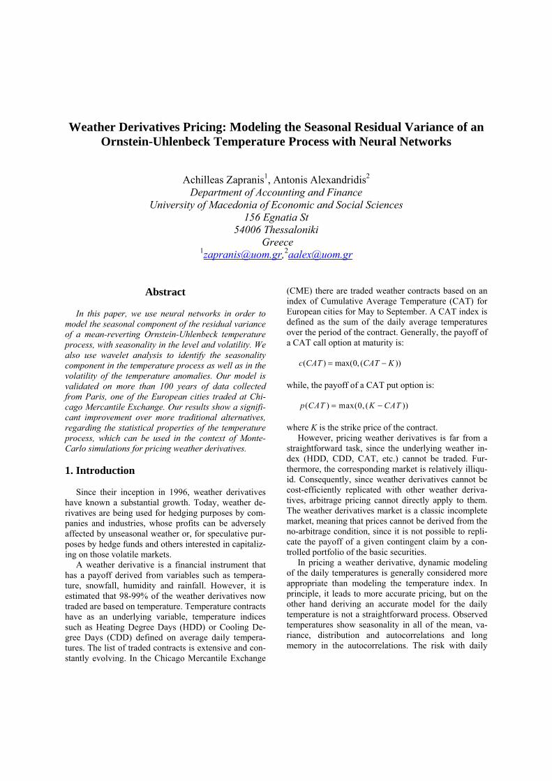
The empirical values of the variance of the residuals (365 values) together with the fitted variance

2 2 2( ) ( )t a tσ σ= (14)

can be seen in Figure 9. We observe that the variance takes its highest values during the winter months, while it takes its lowest values during early Autumn.

The standard deviation of the residuals is 0.6035, while the standard deviation of the remaining noise part is 1.0003 and its mean is 0.0018.

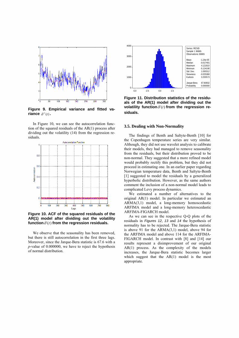
Figure 9. Empirical variance and fitted va-riance )(~ 2 tσ .

In Figure 10, we can see the autocorrelation func-

tion of the squared residuals of the AR(1) process after dividing out the volatility (14) from the regression re-siduals.

Figure 10. ACF of the squared residuals of the AR(1) model after dividing out the volatility function )(~ tσ from the regression residuals.

We observe that the seasonality has been removed, but there is still autocorrelation in the first three lags. Moreover, since the Jarque-Bera statistic is 67.6 with a p-value of 0.000000, we have to reject the hypothesis of normal distribution.

Figure 11. Distribution statistics of the residu-als of the AR(1) model after dividing out the volatility function )(~ tσ from the regression re-siduals.

3.5. Dealing with Non-Normality

The findings of Benth and Saltyte-Benth [10] for

the Copenhagen temperature series are very similar. Although, they did not use wavelet analysis to calibrate their models, they had managed to remove seasonality from the residuals, but their distribution proved to be non-normal. They suggested that a more refined model would probably rectify this problem, but they did not proceed in estimating one. In an earlier paper regarding Norwegian temperature data, Benth and Saltyte-Benth [1] suggested to model the residuals by a generalized hyperbolic distribution. However, as the same authors comment the inclusion of a non-normal model leads to complicated Levy process dynamics.

We estimated a number of alternatives to the original AR(1) model. In particular we estimated an ARMA(3,1) model, a long-memory homoscedastic ARFIMA model and a long-memory heteroscedastic ARFIMA-FIGARCH model.

As we can see in the respective Q-Q plots of the residuals in Figures 12, 13 and 14 the hypothesis of normality has to be rejected. The Jarque-Bera statistic is above 91 for the ARMA(3,1) model, above 94 for the ARFIMA model and above 114 for the ARFIMA-FIGARCH model. In contrast with [8] and [14] our results represent a disimprovement of our original AR(1) process. As the complexity of the models increases, the Jarque-Bera statistic becomes larger which suggest that the AR(1) model is the most appropriate.

0

1000

2000

3000

4000

-5.0 -2.5 0.0 2.5

Series: RESIDSample 1 36865Observations 36865

Mean -1.24e-05Median -0.017401Maximum 4.121810Minimum -5.124190Std. Dev. 1.000312Skewness -0.025360Kurtosis 3.203573

Jarque-Bera 67.60832Probability 0.000000

Figure 12. Q-Q plot of the residuals of an AR-MA(3,1) model.

Figure 13. Q-Q plot of the residuals of an AR-FIMA model.

Figure 14. Q-Q plot of the residuals of an AR-FIMA-FIGARCH model.

Concluding, although the AR(1) model probably is

not the best model for describing temperature anomalies, increasing the model complexity (ARMA, ARFIMA, ARFIMA-FIGARCH) and thus the complexity of theoretical derivations in the context of weather derivative pricing does not seem to be justified.

4. Modeling the Seasonal Residual Va-riance with Neural Networks

Next, we model the seasonal residual variance with a backpropagation neural network, with one hidden layer, a bias term and ten hidden units (Figure 15). For a single-hidden-layer architecture, the number of hid-den units λ is an unambiguous descriptor of the dimen-sionality p of the parameter vector; p = (m + 2)λ + 1. In this case p = (10 + 2)10 + 1 = 121. The corresponding number of observations/parameters ratio is relatively low (n/p = ∼3). 4.1. The Neural Network Model

Our hypothesis here is that between the seasonal

variance and the ten harmonics identified by the wave-let analysis there is a deterministic relationship φ(•) of the general form:

2 ( ) (sin(2 / 365),sin(4 / 365),sin(8 / 365),sin(18 / 365),sin(36 / 365),cos(2 / 365),cos(4 / 365),cos(8 / 365),cos(18 / 365) ,cos(36 / 365))

t t tt t

t tt tt t

σ ϕ π ππ ππ ππ ππ π

=

(15)

We estimate φ(•) non-parametrically with the neural

network g(•). Given an input vector x (the harmonics) and a set of weights w (parameters), the network re-sponse (output) gλ(x;w) is:

⎟⎟⎠

⎞⎜⎜⎝

⎛+⎟

⎠

⎞⎜⎝

⎛+= +

= =+∑ ∑ ]2[

11 1

]1[,1

]1[]2[);( λ

λ

λ γγ wwxwwgj

m

ijmiijjwx (16)

where, w[1]

i,j is a weight corresponding to the connec-tion between the ith input and the jth hidden unit, w[1]

m+1,j is a bias term corresponding to the jth hidden unit, w[2]

j is the weight of the connection between the jth hidden unit and the output unit, and w[2]

λ+1 is the bias term of the output unit, and the function γ(•) is a sig-moidal function.

Figure 15. A neural network for modelling the seasonal residual variance.

An estimate of the parameter vector w is obtained

by minimising iteratively the ordinary least squares cost functional:

( ) ( )( )22

1

1( ) ;2

n

n tt

L t gn

σ=

= −∑w x w (17)

where σ2(t) is the tth target output variance and n is the number of training vectors (365). The loss function in (17) gives us a measure of accuracy with which the estimator fits the observed data but it does not account for the estimator’s (model) complexity. Given a suffi-ciently large number of free parameters, p, the neural estimator can fit the data with arbitrary accuracy. 4.2. Removing the Irrelevant Connections

Once, the parameters of the neural model (16) are estimated, we have to deal with the presence of flat minima (potentially many combinations of the network parameters corresponding to the same level if the em-pirical loss), especially if the statistical properties of the model are of importance, as it is the case in this complex financial application. In order to identify a locally unique solution, we have to remove all the irre-levant parameters, that is the parameters that do not affect the level of the empirical loss.

For this purpose we use the Irrelevant Connection Elimination scheme (ICE) [15], which is much less computationally demanding than other alternatives

since, although it uses the full Hessian of Ln, it does not require inverting the Hessian matrix – a common re-quirement of other algorithms. ICE is based on the Taylor’s approximation of the empirical loss:

( (( )

2

1 1

3

1,

12

12

p p

n i i ii ii i

p

ij i ji i j

L g w a w

a w w O w

δ δ δ

δ δ δ

= =

= ≠

= +

+ +

∑ ∑

∑ (18)

From (18) ICE derives the “saliencies” S(wi), i.e.,

the contribution of wi to δLn, when a small perturbation δwk is added to all connections. as:

S w g w a w wi i i ij i jj

p

( ) = +=∑δ δ δ

1

2 1

(19)

where, δL S wn ii

p

==∑ ( )

1

.

At a well-defined local minimum (19) can be sim-

plified by setting gi = 0, although this is not a require-ment. The method can be summarised in the following steps: Step 1: Train to convergence. Step 2: Compute the saliencies S wi( ) Step 3: Deactivate the connection with the least asso-ciated saliency, unless it was reactivated in step 5. When a pre-specified maximum number of steps is been reached, then the algorithm STOPS. Step 4: Train further for a small number of epochs, until the training error has stabilised. Step 5: If the training error has increased, reactivate the connection, otherwise remove it. Then go to step 3.

Because of possible dependencies in the connec-tions, it is not advisable to remove more than one con-nection at a time (the removal of one connection can affect the standard errors and saliencies of others). This does not pose any computational problems to ICE, since computing the Hessian is the same order of com-plexity as computing the derivatives ∂Ln/∂wi during training.

After applying the algorithm ICE to the estimated network, the number of parameters is reduced to 29 out of 121 originally. The observations/parameters ratio now takes the value of n/p = 12.6 (from 3 originally). Roughly speaking, the reduced network is the same order of complexity with a fully connected network with two hidden units.

4.3. Statistics for the Neural Model and the Re-siduals of the Ornstein-Uhlenbeck Process

The summary statistics for the reduced neural mod-el of the seasonal variance (removing the irrelevant connections) are given in Table 1. As we can see, the coefficient of determination (R2) of the model (adjusted for degrees of freedom), as well as the R2 of the linear regression of the predicted variances vs. the target variances are quite high.

Table 1: Neural Model Summary Statistics Average Squared Error (ASE) 0.007778 Standard error of the estimate (SE) 0.088193 Mean absolute error (MAE) 0.070264 Empirical loss (Ln) 0.003889 Generalised Cross Validation (GCV) 0.017405 Final Prediction Error (FPE) 0.015492 R-squared 64.63906 R-squared (adjusted for d.f.) 59.22428 R-squared for the linear regression of forecasted variance vs. target variance 64.97905

In Table 2 we can see the variable significance sta-

tistics for the network inputs (the input X1 corresponds sin(2πt/365), and so on). The relevance S of the input variables to the model is quantified by the partial de-rivative of the empirical loss (17) to this variable. The sampling variance of the relevance metric is quantified by performing random sampling from the limiting joint distribution of the parameters (it is assumed multivari-ate normal). For more details on this technique refer to [16].

Table 2: Neural Model Variable Significance Estimation Statistics

VAR S=dLn/dX St.Dev. t-value X7 0.00243 0.00020 12.37317 X1 0.00184 0.00014 13.00622 X6 0.00184 0.00014 12.89321 X2 0.00158 0.00316 0.49970 X10 0.00129 0.00259 0.49982 X3 0.00091 0.00006 15.16516 X4 0.00076 0.00005 16.57073 X8 0.00057 0.00114 0.49975 X9 0.00024 0.00007 3.65349 X5 0.00006 0.00011 0.50023

Input variables in Table 2 are sorted in descenting magnitude of the relevance metric S. The most impor-

tant and statistically significant variables appear to be X7, X1, X6, X3, X4 and X9, i.e.,

cos(4πt/365) sin(2πt/365) cos(2πt/365) sin(8πt/365) sin(18πt/365) cos(18πt/365) According to this, the one year cycle (the terms con-

taining 2πt) and the 1/9th of a year cycle (the terms containing 18πt) appear to be significant. The half year cycle (the term containing 4πt) and the 1/4th of the year cycle (term containing 8πt) also appear to be signifi-cant. We also note that since the input cos(2πt/365) does not appear to be significant, the half year cycle takes its highest value at the beginning of each year. Also since the input cos(8πt/365) does not appear to be significant, the 1/4th of the year cycle takes the value of zero at the beginning of each year.

Proceeding now to the analysis of the residuals of the Ornstein-Uhlenbeck temperature process, when using the neural network for estimating nonparameti-cally the seasonal variance, the first thing we observe in the ACF of the residuals (Figure 16) is that the first three lags are significant. This is in line with the ob-served behaviour of the temperature series.

Figure 16. ACF of the squared residuals of the Neural Network after dividing out the volatility function )(~ tσ from the regression residuals.

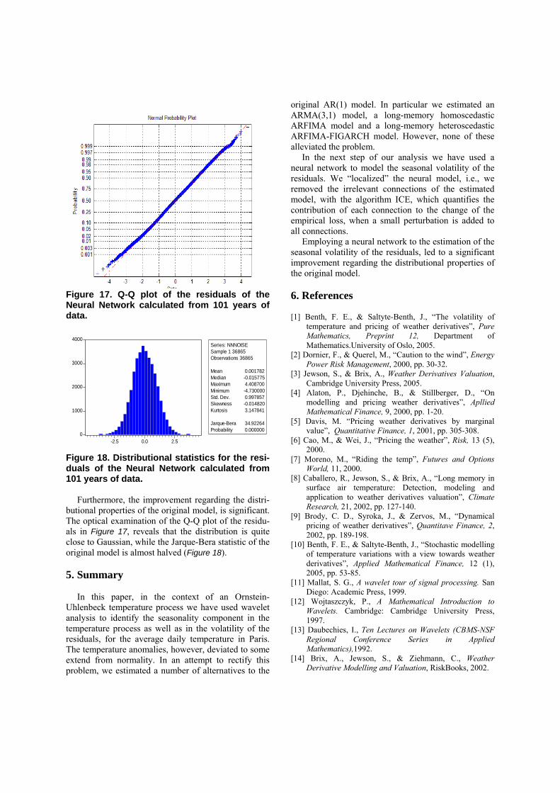
Figure 17. Q-Q plot of the residuals of the Neural Network calculated from 101 years of data.

Figure 18. Distributional statistics for the resi-duals of the Neural Network calculated from 101 years of data.

Furthermore, the improvement regarding the distri-butional properties of the original model, is significant. The optical examination of the Q-Q plot of the residu-als in Figure 17, reveals that the distribution is quite close to Gaussian, while the Jarque-Bera statistic of the original model is almost halved (Figure 18). 5. Summary

In this paper, in the context of an Ornstein-Uhlenbeck temperature process we have used wavelet analysis to identify the seasonality component in the temperature process as well as in the volatility of the residuals, for the average daily temperature in Paris. The temperature anomalies, however, deviated to some extend from normality. In an attempt to rectify this problem, we estimated a number of alternatives to the

original AR(1) model. In particular we estimated an ARMA(3,1) model, a long-memory homoscedastic ARFIMA model and a long-memory heteroscedastic ARFIMA-FIGARCH model. However, none of these alleviated the problem.

In the next step of our analysis we have used a neural network to model the seasonal volatility of the residuals. We “localized” the neural model, i.e., we removed the irrelevant connections of the estimated model, with the algorithm ICE, which quantifies the contribution of each connection to the change of the empirical loss, when a small perturbation is added to all connections.

Employing a neural network to the estimation of the seasonal volatility of the residuals, led to a significant improvement regarding the distributional properties of the original model. 6. References [1] Benth, F. E., & Saltyte-Benth, J., “The volatility of

temperature and pricing of weather derivatives”, Pure Mathematics, Preprint 12, Department of Mathematics.University of Oslo, 2005.

[2] Dornier, F., & Querel, M., “Caution to the wind”, Energy Power Risk Management, 2000, pp. 30-32.

[3] Jewson, S., & Brix, A., Weather Derivatives Valuation, Cambridge University Press, 2005.

[4] Alaton, P., Djehinche, B., & Stillberger, D., “On modelling and pricing weather derivatives”, Apllied Mathematical Finance, 9, 2000, pp. 1-20.

[5] Davis, M. “Pricing weather derivatives by marginal value”, Quantitative Finance, 1, 2001, pp. 305-308.

[6] Cao, M., & Wei, J., “Pricing the weather”, Risk, 13 (5), 2000.

[7] Moreno, M., “Riding the temp”, Futures and Options World, 11, 2000.

[8] Caballero, R., Jewson, S., & Brix, A., “Long memory in surface air temperature: Detection, modeling and application to weather derivatives valuation”, Climate Research, 21, 2002, pp. 127-140.

[9] Brody, C. D., Syroka, J., & Zervos, M., “Dynamical pricing of weather derivatives”, Quantitave Finance, 2, 2002, pp. 189-198.

[10] Benth, F. E., & Saltyte-Benth, J., “Stochastic modelling of temperature variations with a view towards weather derivatives”, Applied Mathematical Finance, 12 (1), 2005, pp. 53-85.

[11] Mallat, S. G., A wavelet tour of signal processing. San Diego: Academic Press, 1999.

[12] Wojtaszczyk, P., A Mathematical Introduction to Wavelets. Cambridge: Cambridge University Press, 1997.

[13] Daubechies, I., Ten Lectures on Wavelets (CBMS-NSF Regional Conference Series in Applied Mathematics),1992.

[14] Brix, A., Jewson, S., & Ziehmann, C., Weather Derivative Modelling and Valuation, RiskBooks, 2002.

0

1000

2000

3000

4000

-2.5 0.0 2.5

Series: NNNOISESample 1 36865Observations 36865

Mean 0.001782Median -0.015775Maximum 4.408700Minimum -4.730000Std. Dev. 0.997857Skewness -0.014820Kurtosis 3.147841

Jarque-Bera 34.92264Probability 0.000000

[15] Zapranis, A., & Haramis, G., “Obtaining locally identified models: The irrelevant connection elimination scheme”, in the proc. of HERCMA 2001.

[16] Zapranis, A., & Refenes, A.-P., Principles of Neural Model Identification, Selection and Adequacy: With Applications to Financial Econometrics, Springer-Verlag, 1999.