Embed Size (px)
Citation preview

Ornstein-Uhlenbeck Equations
with time-dependent coecients
and Lévy Noise
in nite and innite dimensions.
Diplomarbeit
vorgelegt von Florian Knäble
im Studiengang Wirtschaftsmathematik
Fakultäten für
Mathematik und Wirtschaftswissenschaften
Universität Bielefeld
Dezember 2008


Contents
1 Introduction 1
2 Introduction to Lévy Processes 32.1 Lévy Processes . . . . . . . . . . . . . . . . . . . . . . . . . . 3
2.1.1 The Path Structure of Lévy Processes . . . . . . . . . . 82.2 The Lévy-Ito Decomposition . . . . . . . . . . . . . . . . . . . 12
3 Ornstein-Uhlenbeck Processes 293.1 Stochastic Integration . . . . . . . . . . . . . . . . . . . . . . 293.2 Stochastic Convolution . . . . . . . . . . . . . . . . . . . . . . 343.3 Existence of the Mild Solution . . . . . . . . . . . . . . . . . . 353.4 Existence of the Weak Solution . . . . . . . . . . . . . . . . . 37
4 Semigroup and Invariant Measure 414.1 Preliminaries . . . . . . . . . . . . . . . . . . . . . . . . . . . 424.2 Evolution Systems of Measures . . . . . . . . . . . . . . . . . 474.3 The Reduced Equation . . . . . . . . . . . . . . . . . . . . . . 57
4.3.1 The Invariant Measure ν and the Space L2∗(ν) . . . . . 57
4.3.2 Generator and Domain of Uniqueness . . . . . . . . . . 624.4 Asymptotic Behaviour of the Semigroup . . . . . . . . . . . . 65
4.4.1 The Square Field Operator and an Estimate . . . . . . 664.4.2 Functional Inequalities . . . . . . . . . . . . . . . . . . 72
A Cores 81
B Lévy's Continuity Theorem 83
i


Chapter 1
Introduction
The subject of this diploma thesis is the study of an innite dimensionalstochastic dierential equation of Ornstein-Uhlenbeck type with Levy noiseand time-dependent periodic coecients.
Chapter 2 contains a general introduction into Lévy processes with par-ticular emphasis on the Lévy-Ito decomposition and the Lévy-Khinchine rep-resentation.
Taking advantage of the Lévy-Ito decomposition, we establish the neces-sary theory of integration to give sense to our solution in chapter 3.
Then, in chapter 4, we focus our interest on the associated semigroupand in particular on its asymptotic behaviour, its invariant measures and itsgenerator. The equation being non-autonomous results in a two-parametersemigroup, since we have to keep track not only of the elapsed time but alsoof the starting time. In this case the concept of an invariant measure hasto be generalized to allow for a whole collection of measures - a so-calledevolution system of measures- which are invariant in an appropriate sense.We will prove the existence of such a system under some stability conditions.Then we turn the problem into an autonomous one by enlarging the statespace, allowing for a one-parameter semigroup. Via the evolution system ofmeasures and thanks to the periodicity of the coecients we are able to es-tablish a unique invariant measure for this semigroup. Thus we can introducethe L2-space with respect to the invariant measure where the semigroup isstrongly continuous. On a domain of uniqueness for the generator we estab-lish the form of its square eld operator and prove an estimate for it, thatallows us to obtain a Poincaré and a Harnack inequality for our semigroup.This also gives results for the original two-parameter semigroup.
1

2 CHAPTER 1. INTRODUCTION
We will now give an overview of the literature on related problems, whilewe point out our contributions. Our central reference is [daPr/Lun07] whichconcentrates on the nite dimensional case and Gaussian noise. A number ofour arguments are adapted from this paper, although the Lévy setting forcesus to work more heavily with Fourier transforms and the innite dimensionalsetting requires additional care. The existence result on evolution systems ofmeasures (Theorem 4.10) is stated in [daPr/Lun07] in the nite-dimensionalGaussian framework, but the extension to Hilbert spaces and Lévy noise isfundamentally new. The same applies to the existence result on invariantmeasures (Theorem 4.19) for the corresponding one-parameter semigroup .The form of the Fourier transform (Lemma 4.2) and of the generator (Lemma4.24) are also genuine generalizations from what was done in [daPr/Lun07],though they are very close to results from the theory of generalized Mehlersemigroups as for example in [Fuhr/Röck00] or [Lesc/Röck02]. Nevertheless,our framework diers from theirs in that we allow for time-dependent coef-cients, making a direct use of the methods developed there impossible.Our analogue to the integration by parts formula from [daPr/Lun07] is theconcrete calculation of the square eld operator (Lemma 4.30). As far as weknow, there is no such result in our framework, though the general formulain [Lesc/Röck04] is quite similar.The gradient estimate in [daPr/Lun07] corresponds to our estimate of thesquare eld operator, which is a generalization of the result in [Röck/Wang03]to the time-dependent case. Both our proofs of the Poincaré and the Harnackinequality follow the ones in [Röck/Wang03] very closely. Nevertheless, asfar as we know, the extension to our framework is a new result.
The material in chapter 2 and 3 is of course standard, and the referenceswe used can be found at the beginning of each chapter.
I wish to thank Prof. Dr. Michael Röckner for his motivating lectures onstochastic analysis and for his help in connection with this thesis. I wouldalso like to thank Dr. Walter Hoh for his lectures on jump processes andhis help concerning negative denite functions. Finally, special thanks arekindly returned to my brother, Kristian Knäble.

Chapter 2
Introduction to Lévy Processes
2.1 Lévy Processes
The reader well acquainted with Brownian motion, will nd Lévy processesto share at least two of its desired properties. Stationarity and independenceof increments still hold and, together with stochastic continuity, assure thatthe whole process can be characterized simply by its distribution after axed time span. While Brownian motion is characterized by its drift termand covariance operator, it turns out, that, to incorporate the jumps of aLévy process, it is sucient to add a third quantity : the Lévy measure. Thecorrespondence between Lévy processes and these triples is made precisein the seminal Lévy-Khinchine formula 2.36. The Lévy measure codes theinformation about the size and the likelihood of jumps. This measure willin general not be a probability measure, it need not even be nite, howeverit is only allowed to "explode" around zero, illustrating the possibility of anaccumulation point of jumps of vanishing size. Jumps above a xed size,on the other hand, cannot accumulate, an important observation on thepath structure, that will be stated in proposition 2.13, and follows directlyfrom the càdlàg property. The nal result in this section will be the Lévy-Ito decomposition, a representation of a Lévy process as an integral withrespect to a so called Poisson Random Measure. This decomposition is mostimportant, as it will be the basis for stochastic integration against Lévyprocesses.Our exposition follows [App04] and [Alb/Rue05]. Unless stated otherwise,proofs are taken from [App04] and only slightly adapted. Note that the
3

4 CHAPTER 2. INTRODUCTION TO LÉVY PROCESSES
Lévy-Khinchine formula and the Lévy-Ito decomposition are of course closelyrelated and that there are basically two dierent approaches to prove them.We follow what might be called the probabilistic approach and what we deemthe more intuitive one. It consists in proving the Lévy-Ito decomposition rstand to derive the Lévy-Khinchine representation with its help. There is alsoan analytic approach that bases everything on the Lévy-Khinchine formulaas for example in [Sato99].
In the following let be H a separable Hilbert space with scalar product〈·, ·〉 := 〈·, ·〉H and norm ‖ · ‖ := ‖ · ‖H .
Denition 2.1 An H-valued stochastic process L adapted to altration (Ft)t≥0 is a Lévy process if and only if
(L0) L(0) = 0 (a.s)
(L1) L has independent increments , i.e.L(t)− L(s) is independent of Fs for all 0 ≤ s < t < ∞
(L2) L has stationary increments, i.e. for all 0 ≤ s < t < ∞L(t)− L(s) has the same distribution as L(t− s)
(L3) L is stochastically continuous, i.e. for all t ≥ 0 and ε > 0 holds
lims→t
P (‖L(s)− L(t)‖H > ε) = 0
Remark 2.2 We could have required the Lévy process to have càdlàg pathsby denition, but we prefer to emphasize the result(see [Prott90]), that everyLévy process has a modication that is càdlàg(and indeed still satises (L0)-L(3)). The proof is based on the fact, that every martingale admits a càdlàgmodication. Although not every Lévy process is a martingale (of coursecentralization would ensure this, but note that the rst moment need notexist), this argument can be made to work by considering a related martingale.In the following, when speaking about a Lévy process, we will always mean acàdlàg modication.
As it will be useful later on (e.g. in the proof of the strong Markovproperty) we will introduce the martingale mentioned in the remark.

2.1. LÉVY PROCESSES 5
Lemma 2.3 For any xed u ∈ H the process
Mu(t) :=expi〈u, Lt〉
E[expi〈u, Lt〉]
is a martingale.
Although, the numerator is certainly integrable, we now have to rule out thatthe denominator vanishes. This will be done in two additional lemmas whichwill give us some insight into the behaviour of the Fourier transforms of Lt
as t changes and are interesting in themselves.In the following we will denote by ΦX(u) the Fourier transform of a randomvariable X.
Lemma 2.4 For a Lévy process Lt, the map t 7→ ΦLt(u) is continuous foreach u ∈ H.
Proof We have to show
lims→t
E[exp(i〈u, Ls〉)] = E[exp(i〈u, Lt〉)]
Note, simply, that x 7→ exp(i〈u, x〉) is bounded and continuous, and thatconvergence in probability implies convergence in distribution for Hilbertspace valued random variables.
Lemma 2.5 (Lévy symbol) If L is a Lévy process, then for every u ∈ H:
ΦLt(u) = exp(tλ(u))
where λ : H → C.
Proof We will show that for every u ∈ H, t 7→ ΦLt(u) fullls the func-tional equation of the exponential function. We recall that the functionalequation is characterising, that is we prove the following claim :
Claim A function f : R+ → C with the properties:
• f(0) = 1
• f(t + s) = f(t)f(s) ∀s, t ∈ R+

6 CHAPTER 2. INTRODUCTION TO LÉVY PROCESSES
• t 7→ f(t) is continuous
is of the form f(t) = ezt for some z ∈ C.
Proof (of the claim) We must have f 6= 0 everywhere since f(t) = 0would imply f( t
n)n = 0 for every n and hence f( t
n) = 0 for every n but this is
impossible by continuity. So we may dene g(t) := log(f(t)) where log is thebranch of the logarithm that assigns 0 to 1. But g fullls g(t+s) = g(t)+g(s),is continous and g(0) = 0 and hence we must have g(t) = zt for some z ∈ C.Applying the exponential yields the desired result.
So let us check the three conditions in the claim for t 7→ ΦLt(u).ΦL0(u) = E[exp(0)] = 1 is trivial. By stationarity and independence ofincrements:
ΦLt+s(u) = E[ei〈u,Lt+s〉]
= E[ei〈u,Lt+s−Ls〉ei〈u,Ls〉]
= E[ei〈u,Lt+s−Ls〉]E[ei〈u,Ls〉]
= E[ei〈u,Lt〉]E[ei〈u,Ls〉]
= ΦLt(u)ΦLs(u)
The continuity follows, of course, from the last lemma.Thus the claim applies for every xed u and we have ΦLt(u) = etλ(u), whereλ(u) is the complex parameter that will depend on u.
Remark 2.6 So we have seen that the characteristic function of a Lévy pro-cess vanishes nowhere, since it can be written as an exponential. Moreoverthe exponent simply scales by t and hence the whole process is determinedby a single Fourier transform. The function λ has a very special structure,which will be given by the Lévy-Khinchine formula 2.36 later on. We will callλ the Lévy symbol associated to L.

2.1. LÉVY PROCESSES 7
Proof (of Lemma 2.3)Obviously the rst moment exists (this being the point of the construc-
tion). Furthermore, we have
E[
ei〈u,Lt〉
E[ei〈u,Lt〉]|Fs
]= E
[ei〈u,Lt−Ls〉ei〈u,Ls〉
E[ei〈u,Lt−Ls〉]E[ei〈u,Ls〉]|Fs
]=
ei〈u,Ls〉
E[ei〈u,Ls〉]E[
ei〈u,Lt−Ls〉
E[ei〈u,Lt−Ls〉]|Fs
]=
ei〈u,Ls〉
E[ei〈u,Ls〉]
E[ei〈u,Lt−Ls〉]
E[ei〈u,Lt−Ls〉]= Mu(s)
Lemma 2.7 For a xed x ∈ H 〈L(t), x〉 is a real-valued Lévy process.
Proof Note, that we can consider 〈L(t), x〉 as Fx(L(t)) and Fx is linear andcontinuous.So let L be a Lévy-process. (L0) for Fx(L) is trivial. For (L1) and (L2) uselinearity of Fx and the obvious facts, that if X is independent of a σ-algebra
so is F (X) and that if Xd= Y, thenF (X)
d= F (Y ) for any measurable F . For
(L3) note, that Fx is uniformly continuos, since it is linear. So for a xedε > 0 there is δ > 0 such that ‖z−y‖ < δ implies |Fx(z)−Fx(y)| < ε. Hence,(using A ⊂ B ⇒ Bc ⊂ Ac):
P (|Fx(L(t))− Fx(L(s))| > ε) ≤ P (‖L(t)− L(s)‖ > δ)s→t−→ 0
As for Brownian motion the strong Markov property also holds for Lévyprocesses. Since we will often be interested in stopping times related to jumpoccurences, this result will be crucial for several further proofs.
Proposition 2.8 (Strong Markov property) If L is a Lévy process andT is a stopping time, then, on T < ∞, we have for the processLT
t t≥0 := LT+t − LT :
1. LTt is a Lévy process that is independent of FT
2. LTt
d= Lt
3. LT has càdlàg paths and is FT -adapted

8 CHAPTER 2. INTRODUCTION TO LÉVY PROCESSES
Proof We will give an idea of the proof:Assume, at rst, that T is a bounded stopping time, so we can apply optionalstopping.Let A ∈ FT and recall the martingales Mu(t) = ei〈u,Lt〉e−tλ(u) from 2.3Note that we have written the expectation in the form according to 2.5. Fors < t consider the following equalities:
E[ei〈u,LT+t−LT+s〉
]= E
[ei〈u,LT+t〉e−(T+t)λ(u)
ei〈u,LT+s〉e−(T+s)λ(u)
e(T+t)λ(u)
e(T+s)λ(u)
]= E
[Mu(T + t)
Mu(T + s)e(t−s)λ(u)
]= E
[E[
Mu(T + t)
Mu(T + s)e(t−s)λ(u) | FT+s
]]= e(t−s)λ(u)E
[1
Mu(T + s)E [Mu(T + t) | FT+s]
]= e(t−s)λ(u) = E
[ei〈u,Lt−s〉
]Thus, setting s = 0, we see that LT+t − LT and Lt have the same Fouriertransforms and hence the same distributions and we have proven (2). For aproof of 1. and 3. see [App04] Theorem 2.2.11.
2.1.1 The Path Structure of Lévy Processes
One of the big dierences between Brownian motion and general Lévy pro-cesses is, that the latter do not admit continuous paths. We have, however,pointed out, that their paths are still right continuous and admit left limits.So the only discontinuities that can occur are of jump type. As we will aimto split a Lévy process into a continuous part and a jump part in the Lévy-Ito decomposition, it is worthwhile to take a closer look on the occurence ofjumps. First, we will combine stochastic continuity with the càdlàg propertyto see, that jumps at a xed time occur only with probability 0. Then, againby the càdlàg property, we will show that there are only nitely many jumpson bounded intervals.
Denition 2.9 Let Lt be a Lévy process. Since we always have left limits,let Lt− := limst Ls. We will call ∆Lt := Lt − Lt− the jump of L at time t.Accordingly, we will call the process ∆Ltt>0 the jump process of L.

2.1. LÉVY PROCESSES 9
Lemma 2.10 If L is a Lévy process we have P (∆Lt 6= 0) = 0 for any xedt.
Proof Let tn be an increasing real sequence with limit t. By the càdlàgproperty limn→∞ Ltn = Lt− exists for every ω. On the other hand, by stochas-tic continuity, we obtain a subsequence of tn that converges for almost all ωto Lt. So Lt− = Lt by uniqueness of limits.
Remark 2.11 One may be tempted to assume that ∆L is itself a Lévy pro-cess, but this is false in general. Let Nt be a Poisson process. Then, we haveby the above : P (∆Nt −∆Ns = 0) = 1 since with probability 1 there will beno jumps. On the other hand (and for the same reason) we haveP (∆Nt −∆Ns = 0|∆Ns = 1) = 0. So increments are not independent.
As we pointed out, we want to prove that there are only nitely manyjumps on nite intervals. However, this is only true if we exclude arbitrarysmall jumps. Those might accumulate without contradicting the càdlàg prop-erty. Thus, the following denition is crucial:
Denition 2.12 We say that A ∈ B(H) is bounded below if 0 /∈ AWe denote by N(t, A) the (random) number of "jumps of size A" up to timet, that is N(t, A) := card0 ≤ s ≤ t|∆Ls ∈ A
Proposition 2.13 If L has càdlàg paths and A is bounded below, then N(t, A)is nite for every xed t.
Proof Assume N(t, A) = ∞, so that we have innitely many jumps of sizeA in nite time, which have to accumulate, say at s.We can then nd asequence sn ⊂ 0 ≤ s ≤ t|∆Ls ∈ A tending to s either from the left or fromthe right. As A is bounded below we can nd ε > 0 such that ‖∆Lsn‖ > 2 ε.First assume that sn s. By the càdlàg property there is δ > 0 suchthat ‖Ls − Lr‖ < ε ∀ r with r − s < δ. Take n large enough to assure‖Ls−Lsn‖ < ε. Of course we also have ‖Ls−Lsn−‖ < ε then. By the triangleinequality this implies ‖Lsn − Lsn−‖ < 2 ε contradicting our requirement onA.Note that, in the proof, the value of Ls is arbitrary, we need only that theleft limit exists. So the proof for sn s is the same, with Ls replaced byLs−.

10 CHAPTER 2. INTRODUCTION TO LÉVY PROCESSES
We stress once more that N(t, A) depends on ω. It is easy to see that N(t, A)is a random variable (it will become clear in the proof of the next proposition)and we can hence ask if we can nd out something about its distributionand how it depends on the set A. Moreover, xing only A (which must bebounded below, for technical reasons) and writing NA
t for a more suggestivenotation we want to examine the process NA
t t≥0. Note that N(t, A) onlytakes values in N and that its jumps are always of size 1. Hence one mighthope for a Poisson process, and to show that this is indeed true, we will rstprove an auxiliary characterization result.
Proposition 2.14 If L is a Lévy process that takes values in N only, isalmost surely increasing and has only jumps of size 1, then L is a Poissonprocess.
Proof The idea is to show that the waiting times between jumps are ex-ponentially distributed, by using the characteristical functional equation ofthe exponential again (compare the proof of 2.5). Let be Tn the sequence ofstopping times, dened by Tn := inft > 0 |Lt = n. Tn is a stopping timebecause of Tn ≤ t = Lt > 0. From 2.8 (strong Markov property) weget that the random variables T1, T2 − T1, T3 − T2, ... are independent andidentically distributed. On the other hand by stationarity and independenceof the increments of L we have:
P (T1 > s + t) = P (Ls = 0, Ls+t − Ls = 0)
= P (Ls = 0) P (Ls+t − Ls = 0)
= P (Ls = 0) P (Lt = 0)
= P (T1 > s) P (T1 > t)
So f(t) = P (Lt > 0) fullls f(t + s) = f(t)f(s) ∀ t, s > 0. Furthermore, wehave:f(0) = P (T1 > 0) = P (L0 = 0) = 1 andf(t) = P (Lt = 0) = 1− P (Lt ≥ 1) = 1− P (|Lt − L0| ≥ 1) → 1 as t → 0because of stochastic continuity, so f is continuous in 0 and sincef(t + s)− f(s) = f(s)(f(t)− 1) we have at least right continuity of f , whichallows us to deduce that f(t) = eαt for some α ∈ R. Moreover we havef(t) < 1 for some t, otherwise we would have 1 = P (T1 > t) = P (Lt = 0)∀ tcontradicting the assumption that Lt is increasing. So −β := α must be

2.1. LÉVY PROCESSES 11
negative. Having P (T1 > t) = e−βt, we get P (T1 ≤ t) = 1 − e−βt anddierentiation yields the density ρT1(t) = βe−βt, thus T1 is exponentiallydistributed. It is then well-known that Lt must be a Poisson process.
Proposition 2.15 If A is bounded below, then NAt is a Poisson process.
Proof By the characterization above, we only have to show that NAt is
a Lévy Process. We can assume that NAt is increasing, otherwise NA
t willjust be the zero process, which we will consider as a Poisson process withintensity 0. (L0) is clear, since by 2.10 with probability 1 we have no jumpat 0. (L1) and (L2) follow directly from the respective properties of Lt.Stochastic continuity, on the other hand, is astonishingly dicult to prove.Since N(t, A) = 0 implies N(s, A) = 0 for all s < t we have for n ∈ N:
P [N(t, A) = 0] = P
[N
(t
n, A
)= 0, N
(2t
n, A
)= 0, . . . , N(t, A) = 0
]= P
[N
(t
n, A
)= 0, N
(2t
n, A
)−N
(t
n, A
)= 0, . . .
. . . , N(t, A)−N
((n− 1)t
n, A
)= 0
]=
(P
[N
(t
n, A
)= 0
])n
by independent increments
Hence we have :
lim supt→0
P [N(t, A) = 0] = lim supt→0
(P
[N
(t
n, A
)= 0
])n
= limn→∞
lim supt→0
(P
[N
(t
n, A
)= 0
])n
= limn→∞
(lim sup
t→0P
[N
(t
n, A
)= 0
])n
but
lim supt→0
P
[N
(t
n, A
)= 0
]= lim sup
t→0P [N (t, A) = 0]
is independent of n, so it can be only 0 or 1. Since the same argument appliesto the lim inf as well, there are only three possibilities:

12 CHAPTER 2. INTRODUCTION TO LÉVY PROCESSES
1. 0 = lim inft→0 P [N (t, A) = 0] 6= lim supt→0 P [N (t, A) = 0] = 1
2. limt→0 P [N (t, A) = 0] = 0
3. limt→0 P [N (t, A) = 0] = 1
3. implies stochastic continuity, so we will show that the other two are im-possible:As N is an increasing process P [N (t, A) = 0] =: Pt is decreasing in t. As-sume 1. especially lim supt→∞ Pt = 1, so that we must have Pt > 1
2for some
t. But since Pt is decreasing this implies Ps > 12∀ s < t so lim inft→∞ Pt = 0
is impossible.Assume 2. so that equivalently limt→0 P [N (t, A) > 0] = 1 Choose anotherB which is bounded below and disjoint from A. Then P [N (t, A ∪B) > 0] =P [N (t, A) > 0] + P [N (t, B) > 0] so that 2. is impossible, too.
2.2 The Lévy-Ito Decomposition
The aim of this decomposition is to show that we can write every Lévyprocess as a sum of a drift term, a continuous Brownian part and a jump part.The proof of the Lévy-Ito Decomposition illustrates very well the technicaldiculties posed by the jumps. First of all, a Lévy process need not haveany moments and proposition 2.25 will show that this is only due to the bigjumps. Subtracting those, we can centralize and the remaining jump partwill be a martingale, although this is dicult to prove in the case wherethere are arbitrary small jumps. It remains then to show, that the rest termis continuous and a Brownian motion.
In order to nd a convenient representation for the jump part we have tointroduce Poisson integrals. In principle we want to give meaning to some-thing like
∑s≤t f(∆Ls), but this sum might not be nite, even for bounded
f because of an inte number of small jumps , so we have to come up withanother approach in the general case. If we consider only jumps above acertain threshold specied by a set A,which is bounded below, we know thatthe sum above will be nite, as is N(t, A) But then, of course, we will want tomake this threshold arbitrarily small. So we need to investigate the inuenceof A on N(t, A). First of all we note, that jumps of dierent size cannotinuence each other:

2.2. THE LÉVY-ITO DECOMPOSITION 13
Lemma 2.16 If A and B are bounded below and we have A ∩ B = ∅ thenN(t, A) and N(t, B) are independent.
Proof see [App04] Theorem 2.3.5
It is fairly obvious that for xed ω and t Nt(A) is additive for disjointsets. We prove now that it is even a pre-measure on a properly chosen ring.Moreover, as Nt(A) depends on ω we may take expectation, for t xed andit turns out, that we still have a pre-measure.
Denition 2.17 For A bounded below, set ν(A) = E[N(1, A)].Set R := A ⊂ H|A is bounded below and Borel measurable
Lemma 2.18 R is a ring in H\0, and ν and N(t, ·) are pre-measures onR.
Proof To see that R is a ring in H\0 we note that: because of A ∪B ⊂A ∪ B we have, that 0 ∈ A ∪B implies 0 ∈ A or 0 ∈ B so that A ∪ B muststill be bounded below, if A and B are. To see that N(t, ·) is a pre-measureon R, recall that we have to check σ-additivity only for unions that stillbelong to the ring. So let A :=
⋃n An where A and all the An are bounded
below. Then we have:
Nt(⋃n
An) =∑s≤t
χ(S
n An)(∆Xs)
=∑s≤t
∑n
χAn(∆Xs) =∑
n
∑s≤t
χAn(∆Xs) =∑
n
Nt(An)
Note that we could interchange sums as all terms are positive, but that if Awas not bounded below, the second expression might not even make sense.To see that ν(A) is nite for A bounded below, we have to refer to proposition2.25. As Nt(A) is a Lévy process with bounded jumps (of size 1) the rstmoment must exist. The proof for ν then follows the same lines, we justhave to interchange sum and expectation in the last step, which is justiedby monotone convergence.
Proposition 2.19 We can extend ν and N(t, ·) uniquely to σ-nite measureson the σ-algebra S := A ⊂ H|A is Borel and 0 /∈ A in H\0
14 CHAPTER 2. INTRODUCTION TO LÉVY PROCESSES
Proof To make use of Caratheodory we have to show, that ν and Nt areσ-nite on R and that R generates S. But both follows easily on consideringthe sets An := x ∈ H| ‖x‖ ≥ 1
n which are in R .
Remark 2.20 The measure ν is indeed the third member of the character-ising triple, mentioned in the introduction. Heuristically, we can already un-derstand that it contains all the information necessary to describe the jumpstructure. Imagine, we wanted to roughly simulate the jump process of a Lévyprocess. We would try to cover the space H with suciently small and disjointsets. Then we would simulate a collection of independent (recall proposition2.16) Poisson processes, one for each set, giving us the respective jump times.Each Poisson process is characterized by its intensity parameter and this isprecisely provided by ν, as we state in the next simple lemma.
Lemma 2.21 If A is bounded below, Nt(A)d= π(tν(A)) , where π(c) is the
Poisson distribution with parameter c. Moreover the process Nt(A) − tν(A)is a martingale.
Proof The intensity of a Poisson process Pt is given by E[P1]. Hence ν givesthe intensity by construction. The second result follows by noting that anyadapted independent-increment process that is centralized is a martingale.
The most important properties of Nt(·) are summarized in the next de-nition.
Denition 2.22 Let (S,A) be a measurable space. A Poisson random mea-sure is a collection of random variables N(A)A∈A on a common probabilityspace Ω such that
• for almost all ω N(·) is a measure on (S,A)
• if A1, ..., An are mutually disjoint, the random variables N(A1), ..., N(An)are independent
• whenever E[N(A)] < ∞ N(A) has a Poisson distribution
Remark 2.23 As ν is somehow compensating the drift of Nt, we will callthe random measure Nt − tν the compensated Poisson random measure.

2.2. THE LÉVY-ITO DECOMPOSITION 15
As Nt(·) is a measure on H\0 for ω xed we may dene,for f : H → H measurable
∫A
f(x)Nt(dx) as a random Bochner integral.For a short account on Bochner integrals see appendix A of [Spde07].The following proposition explores the properties of this integral as a randomvariable in terms of its Fourier transform and its rst two moments. In[App04] this is Theorem 2.3.8 , that we have adapted to the Hilbert spacesetting and where we made the proof of 2. and 3. rigorous.
Proposition 2.24 Let A be bounded below and∫
A‖f(x)‖ ν(dx) < ∞, then:
1.
E[exp
(i
⟨u,
∫A
f(x)Nt(dx)
⟩)]= exp
(t
∫A
(ei〈u,x〉 − 1
)ν f−1(dx)
)
2.
E[∫
A
f(x)Nt(dx)
]= t
∫A
f(x)ν(dx)
3. moreover, if∫
A‖f(x)‖2 ν(dx) < ∞:
Var
[‖∫
A
f(x)Nt(dx)‖]
= t
∫A
‖f(x)‖2ν(dx)
Proof 1. First, let f be a simple function, f =∑n
j=1 hjχAjwhere hj ∈ H
and the Aj are disjoint measurable subsets of A. Then by 2.16 N(t, Aj)

16 CHAPTER 2. INTRODUCTION TO LÉVY PROCESSES
and N(t, Ai) are independent and so we have:
E[exp
(i
⟨u,
∫A
f(x)Nt(dx)
⟩)]=E
[exp
(i
⟨u,
n∑j=1
hjNt(Aj)
⟩)]
=E
[n∏
j=1
exp (i 〈u, hjNt(Aj)〉)
]
=n∏
j=1
E [exp (i 〈u, hjNt(Aj)〉)]
=n∏
j=1
E [exp (i 〈u, hj〉Nt(Aj))]
=n∏
j=1
exp(t[ei〈u,hj〉 − 1
]ν(Aj)
)= exp
(n∑
j=1
t[ei〈u,hj〉 − 1
]ν(Aj)
)
= exp
(t
∫A
[ei〈u,f(x)〉 − 1
]ν(dx)
)
So we have the result for simple functions. For every integrable f wecan nd a sequence of simple functions fn, that converge pointwise tof , so we have:
limn→∞
exp
(t
∫A
[ei〈u,fn(x)〉 − 1
]ν(dx)
)= exp
(t
∫A
[ei〈u,f(x)〉 − 1
]ν(dx)
)by dominated convergence. On the other hand we obtain
limn→∞
E[exp
(i
⟨u,
∫A
fn(x)Nt(dx)
⟩)]=
E[exp
(i
⟨u,
∫A
f(x)Nt(dx)
⟩)]

2.2. THE LÉVY-ITO DECOMPOSITION 17
as follows: If we can show that for P−almost all ω :
limn→∞
∫A
fn(x)Nt(dx)(ω) =
∫A
f(x)Nt(dx)(ω) (2.1)
then dominated convergence gives again the result. But (2.1) will followif:
limn→∞
∫A
‖fn(x)− f(x)‖Nt(dx)(ω) = 0 (2.2)
and we will show this by dominated convergence. By assumption wehave:
∞ > t
∫A
‖f(x)‖ν(dx) =
∫A
E[‖f(x)‖Nt(dx)] = E[∫
A
‖f(x)‖Nt(dx)
]where we used Fubini-Tonelli.Hence we must have
∫A‖f(x)‖Nt(dx) < ∞ almost surely, and since Nt
is for any xed ω a nite measure, we can take 2‖f(x)‖ + const as auniform bound in (2.2) for almost all ω.Note that the technical problems arise from the fact, that the measurefor the Bochner integral does depend on ω, but our sequence of simplefunctions must not.
2. First assume that f is bounded, that is supx∈H ‖f(x)‖ = M < ∞.For λ ∈ R we will consider the rst identity for λf , then dierentiatewith respect to λ and set λ = 0:
d
dλE[exp
(λi
⟨u,
∫A
f(x)Nt(dx)
⟩)]=
d
dλexp
(t
∫A
(eλi〈u,f(x)〉 − 1
)ν(dx)
)Starting with the right hand side, we get by formally interchangingderivation and integration:
d
dλ
∣∣∣∣λ=0
exp
(t
∫A
(eλi〈u,f(x)〉 − 1
)ν(dx)
)= t
∫A
i〈u, f(x)〉ν(dx)
= i〈u, t
∫A
f(x)ν(dx)〉
18 CHAPTER 2. INTRODUCTION TO LÉVY PROCESSES
where we have also used that the Bochner integral commutes with thescalar product, as it is linear and continuous for xed u and becausef is integrable. Derivation under the integral is justied because thederived integrand is uniformly integrable in λ:
supλ
∫A
∣∣(eλi〈u,f(x)〉 − 1)i〈u, f(x)〉
∣∣ ν(dx) ≤ 2
∫A
|〈u, f(x)〉| ν(dx)
≤ 2‖u‖∫
A
‖f(x)‖ν(dx) < ∞
For the left hand side we can interchange derivation and expectationlikewise, since:
supλ
E∣∣∣∣exp
(λi
⟨u,
∫A
f(x)Nt(dx)
⟩)i
⟨u,
∫A
f(x)Nt(dx)
⟩∣∣∣∣≤ E
∣∣∣∣⟨u,
∫A
f(x)Nt(dx)
⟩∣∣∣∣ ≤ E[‖u‖M
∫A
Nt(dx)
]= ‖u‖M E[Nt(A)] = ‖u‖Mtν(A) < ∞
Thus we obtain:
d
dλ
∣∣∣∣λ=0
E[exp
(λi
⟨u,
∫A
f(x)Nt(dx)
⟩)]
= E[i
⟨u,
∫A
f(x)Nt(dx)
⟩]= i
⟨u, E
[∫A
f(x)Nt(dx)
]⟩So we have
i
⟨u, E
[∫A
f(x)Nt(dx)
]⟩= i〈u, t
∫A
f(x)ν(dx)〉
for arbitrary u ∈ H and the result follows for bounded f . For merelyintegrable f we set fn := fχ‖f‖≤n so that fn is bounded and fn fpointwise. To complete the proof, we have to show that:
E[∫
A
f(x)Nt(dx)
]= E
[∫A
limn→∞
fn(x)Nt(dx)
]!= lim
n→∞E[∫
A
fn(x)Nt(dx)
]
= limn→∞
t
∫A
fn(x)ν(dx)!= t
∫A
limn→∞
fn(x)ν(dx) = t
∫A
f(x)ν(dx)

2.2. THE LÉVY-ITO DECOMPOSITION 19
To see that we may interchange limit and integrals we show
E[∫
A
‖fn(x)− f(x)‖Nt(dx)
]n→∞−→ 0
by dominated convergence. As ‖fn‖ ≤ ‖f‖, 2‖f‖ is an upper bound,and we have by Fatou:
E[∫
A
‖f(x)‖Nt(dx)
]= E
[∫A
limn→∞
‖fn(x)‖Nt(dx)
]≤ E
[lim infn→∞
∫A
‖fn(x)‖Nt(dx)
]≤ lim inf
n→∞E[∫
A
‖fn(x)‖Nt(dx)
]= lim inf
n→∞t
∫A
‖fn(x)‖ν(dx) =
∫A
‖f(x)‖ν(dx) < ∞
since ‖f‖ is ν-integrable by assumption. This also implies:
∫A
‖fn(x)− f(x)‖ν(dx)n→∞−→ 0
and thus the last interchange is also justied.
3. We make the same approach dierentiating twice with respect to λand setting λ = 0. Note that since ν(A) < ∞ for A bounded below,the assumption from 2. is now valid as well. Unlike in 2. we directlyconsider a non-bounded f and we obtain along the same lines:
d2
dλ2
∣∣∣∣λ=0
exp
(t
∫A
(eλi〈u,f(x)〉 − 1
)ν(dx)
)=
(ti〈u,
∫A
f(x)ν(dx)〉)2
+
∫A
(ti〈u, f〉)2ν(dx)
where we used the assumption to justify derivation under the integral.So we have seen that the characteristic function is twice dierentiablein 0. Borrowing a trick from [Chung68] we will show now that this
20 CHAPTER 2. INTRODUCTION TO LÉVY PROCESSES
implies the existence of second moments for X := 〈u,∫
Af(x)Nt(dx)〉.
E[|〈u, X〉|2
]= 2E
[limh→0
1− cos(h〈u, X〉)h2
]by Taylor expansion of the cosine
≤ lim infh→0
E[2− 2 cos(h〈u, X〉)
h2
]by Fatou
= lim infh→0
E[2− eih〈u,X〉 − e−ih〈u,X〉
h2
]by Euler's formula
= − d2
dλ2
∣∣∣∣λ=0
E[eλi〈u,X〉] by central approximation ofd2
dλ2
< ∞ as we pointed out above
Thus the next interchange is also in order:
d2
dλ2E[exp
(λi
⟨u,
∫A
f(x)Nt(dx)
⟩)]= E
[(i
⟨u,
∫A
f(x)Nt(dx)
⟩)2]
As u is arbitrary we now take u = en for an orthonormal basis enn∈Nand sum over n, using Parseval's identity:
∞∑n=1
(t
⟨en,
∫A
f(x)ν(dx)
⟩)2
=∞∑
n=1
(⟨en, E
[∫A
f(x)Nt(dx)
]⟩)2
=
∥∥∥∥E [∫A
f(x)Nt(dx)
]∥∥∥∥2
where we have employed 2.∞∑
n=1
∫A
t(〈en, f〉)2ν(dx) =
∫A
∞∑n=1
t(〈en, f〉)2ν(dx) =
∫A
t‖f‖2ν(dx)
where we have interchanged summation and integration by monotoneconvergence.
∞∑n=1
E
[(⟨en,
∫A
f(x)Nt(dx)
⟩)2]
=
E
[∞∑
n=1
(⟨en,
∫A
f(x)Nt(dx)
⟩)2]
= E
[∥∥∥∥∫A
f(x)Nt(dx)
∥∥∥∥2]

2.2. THE LÉVY-ITO DECOMPOSITION 21
where we have interchanged summation and expectation by Fubini-Tonelli. So we have:
E
[∥∥∥∥∫A
f(x)Nt(dx)
∥∥∥∥2]
=
∥∥∥∥E [∫A
f(x)Nt(dx)
]∥∥∥∥2
+
∫A
t‖f(x)‖2ν(dx)
and recalling that Var[‖X‖] = E[‖X‖2]− ‖E[X]‖2 we obtain 3.
Proposition 2.25 If L is a Lévy process with bounded jumps, then it hasmoments of all orders.
Proof Let J be the bound for the jumps of L. Dene stopping times by :T1 := inft ≥ 0 : ‖Lt‖ > J and Tn := inft ≥ Tn−1 : ‖Lt − LTn−1‖ > J.So we have Tn − Tn−1 = inft > 0 : ‖LTn−1+t − LTn−1‖ > J.By the strong Markov property 2.8 we see that Tn − Tn−1 has the samedistribution as T1, and that Tn−Tn−1 is independent of FTn−1 . So by iteratedoptional stopping:
E[e−Tn ] = E[e−T1e−(T2−T1) · · · e−(Tn−Tn−1)] = (E[e−T1 ])n = qn
for some 0 ≤ q < 1 since 0 ≤ e−T1 ≤ 1 but P (T1 = 0) = 0 since there are nojumps at 0 with probability 1. Furthermore, note that if we have ‖Lt‖ > 2nJthis can only happen on Tn < t. This is clear, since the process can grow onlyby a maximum of 2J between two stopping times, as it is stopped when thedierence exceeds J and a possible jump shortly before the critical point canwin not more than another J by the assumption of bounded jumps. Hence,we get by the Markov inequality:
P (‖Lt‖ ≥ 2nJ) ≤ P (Tn < t) = P (e−Tn > e−t) ≤ E[e−Tn ]et = qnet
So the tail of P‖Lt‖ is so thin, that we may use a rather rough estimate forthe moments m = 1, 2 . . .∫
R+
ym P‖Lt‖(dy) =∞∑
k=0
∫ (k+1)2J
k2J
ymP‖Lt‖(dy)
≤∞∑
k=0
(k + 1)2J P (‖Lt‖ ≥ k2J) ≤ 2J∞∑
k=0
(k + 1)etqk < ∞
22 CHAPTER 2. INTRODUCTION TO LÉVY PROCESSES
Given a general Lévy process, we dene a new process with boundedjumps just by subtracting the big jumps. That this process is still a Lévyprocess is stated in the next lemma.
Denition 2.26 Given a Lévy process L dene L1(t) := L−∫‖x‖>1
xN(t, dx)
Lemma 2.27 L1 is a Lévy process.
Proof see [App04] Theorem 2.4.8
Since without large jumps, we can centralize, dene:
Denition 2.28 L1 := L1 − E[L1]
Since we now have second moments we can use the powerful theory of squareintegrable martingales:
Theorem 2.29 There is a decomposition : L1 = L1c + L1
j such that L1c and
L1j are independent Lévy processes. L1
c has continuous sample paths and
L1j =
∫‖x‖≤1
x [N(t, dx)− tν(dx)] := L2 − limn→∞
∫1n
<‖x‖<1
x [N(t, dx)− tν(dx)]
Proof see [App04] Theorem 2.4.11
Corollary 2.30 For the measure ν we obtain:∫‖x‖≤1
‖x‖2ν(dx) < ∞
Proof∫‖x‖≤1
‖x‖2ν(dx) = limn→∞
∫1n
<‖x‖≤1
‖x‖2ν(dx)
= limn→∞
Var
[∫1n
<‖x‖≤1
x N(1, dx)
]= Var[L1
j ] < ∞
We already know that ν(‖x‖ > 1) < ∞ since it is the intensity of therespective Poisson process (note that ‖x‖ > 1 is bounded below) andhence nite. Thus, we have motivated the following denition:

2.2. THE LÉVY-ITO DECOMPOSITION 23
Denition 2.31 A measure M on H with :∫H\0
min(1, ‖x‖2)M(dx) < ∞
is called a Lévy measure.
Proposition 2.32 A real valued, centred Lévy process Bt with continuoussample paths is a Brownian motion.
Proof We will show that E[eiuBt ] = e−12t2 for some a ≥ 0. As the char-
acteristic function uniquely determines a Lévy process, Bt then must be aBrownian motion.Since Bt has no jumps, all moments exist by proposition 2.25, thus the char-acteristic function ΦBt(u) =: Φt(u) is innitely dierentiable. By lemma 2.5it has the form Φt(u) = etλ(u) for some λ : R → C which hence must be alsosmooth. Moreover we have 0 = iE[Bt] = tλ′(0) and this easily implies
E[Bkt ] = a1t + a2t
2 + ... + ak−1tk−1 (2.3)
for the other moments by repeated dierentiation, where the ak are realconstants. Note that we can already see: E[B2
t ] = a1t and thus, we musthave a1 ≥ 0. Note also that since the quadratic variation of Bt is almostsurely nite, cubic variation will vanish almost surely. Actually this is agood hint why the remainder in the following expansion should vanish.Let P be a partition 0 = t0 < t1 < ... < tn = t and write ∆Bj :=Btj+1
−Btj . We employ Taylor expansion up to second order for the functionf(x) = eiux to get:
E[eiuBt − 1] = E
[n−1∑j=0
(eiuBj+1 − eiuBj)
]=: E[T1 + T2 + TR]
where
T1 = iu
n−1∑j=0
eiuBj∆Bj
T2 = −u2
2
n−1∑j=0
eiuBj(∆Bj)2

24 CHAPTER 2. INTRODUCTION TO LÉVY PROCESSES
TR = −u2
2
n−1∑j=0
(eiuBj+Θj∆Bj − eiuBj)(∆Bj)2
with 0 < Θj < 1, j = 0...n− 1.
T1 and T2 yield easily by idependent increments:
E[T1] = iun−1∑j=0
E[eiuBj ]E[∆Bj] = 0
and
E[T2] = −u2
2
n−1∑j=0
E[eiuBj ]E[(∆Bj)2] = −a1
u2
2
n−1∑j=0
Φtj(u)(tj+1 − tj)
where we have used (2.3) for k = 2. Now rene the partition P , that isconsider a sequence Pn of partitions with limn→∞ supjn
|tjn+1 − tjj| = 0. We
write T n2 for the term with respect to the n-th partition and we have
limn→∞
E[T n2 ] = −a1
u2
2
∫ t
0
Φs(u)ds
So that if limn→∞ E[T nR] = 0 we will have:
Φt(u)− 1 = −a1u2
2
∫ t
0
Φs(u)ds
which yields the result by solving the dierential equation:
d
dtΦt(u) = −a1
u2
2Φt(u)ds Φ0(u) = 1
To show limn→∞ E[T nR] = 0 one could try to use the mean value theorem
to get by |eiu(x+y) − eiux| ≤ |uy|:
limn→∞
E[T nR] ≤ lim sup
n→∞
|u|3
2E
[n−1∑jn=0
|∆Bj|3]
≤ lim supn→∞
|u|3
2supjn,ω
|∆Bjn|E
[n−1∑jn=0
|∆Bj|2]

2.2. THE LÉVY-ITO DECOMPOSITION 25
Indeed E[∑n−1
jn=0 |∆Bj|2]
= a1t independent of n by (2.3). For supjn,ω |∆Bjn|we get limn→∞ supjn
|∆Bjn| = 0 for ω xed by uniform continuity. Unfortu-nately, the modulus of continuity is path-dependent, so the approach doesnot work that fast. Thus, we introduce the set of "good" paths:
Gnε := ω | sup
jn∈Pn
|∆Bjn| < ε
So splitting E[T nR] = E[T n
R 1Gnε] + E[T n
R 1(Gnε )c ] we obtain as above:
E[T nR 1Gn
ε] ≤ εa1t
|u|3
2(2.4)
On the other hand, using |eix| ≤ 1 for a dierent estimate of TR we get:
E[T nR 1(Gn
ε )c ] ≤ E[1(Gnε )cu2
n−1∑jn=0
|∆Bj|2]
≤ u2√
P (1(Gnε )c)
E
( n−1∑jn=0
|∆Bj|2)2 1
2
by Cauchy-Schwarz. But again by (2.3) it is easy to see that we can esti-mate the expectation of the squared sum independent of n. So if we canshow limn→∞ P ((Gn
ε )c) = 0 for every xed ε we are done, since by making εarbitrarily small the right hand side in (2.4) will vanish as well.But as we noted above, for every xed ω, uniform continuity will assure thateventually ω ∈ Gn
ε for n large enough. Hence 1(Gnε )c → 0 for n →∞, so that
P (Gnε )c) → 0 by dominated convergence.
Corollary 2.33 L1c is a Brownian motion.
Proof Since L1c has continuous sample paths, so has 〈L1
c , h〉 for any h ∈ H.Moreover by 2.7 〈L1
c , h〉 is a Lévy process. Hence 〈L1c , h〉 is a real-valued
Brownian motion for any h ∈ H and thus by Proposition 5.2.3 in [Linde83]L1
c is a Wiener process on H.

26 CHAPTER 2. INTRODUCTION TO LÉVY PROCESSES
Theorem 2.34 (Lévy-Ito Decomposition) If L is an H-valued Lévy pro-cess, there is a drift vector b ∈ H, a Q-Wiener process WQ on H, such thatWQ is independent of Nt(A) for any A that is bounded below and we have:
Lt = bt + WQ(t) +
∫‖x‖<1
x(Nt(dx)− tν(dx)) +
∫‖x‖≥1
xNt(dx)
where Nt is the Poisson random measure associated to L, and ν the corre-sponding Lévy measure.
Proof Lemma 2.27 allows to separate the big jumps. Then we can centralizeas in denition 2.28 with :
b = E[L(1)−∫‖x‖<1
x N(1, dx)]
and theorem 2.29 allows to separate the small jumps. Then by corollary 2.33the remainder is a Brownian motion.
Remark 2.35 If∫‖x‖≥1
xNt(dx) has rst moment we can directly centralize
and the form of b would change.However, in general the drift only contains the expectation of the small jumpsand we will retrieve this asymmetry in the Lévy-Khinchine formula in theform of a cut-o function.
Theorem 2.36 (Lévy-Khinchine Representation) If L is an H-valuedLévy process with Lévy-Ito decomposition as in 2.34, then its Lévy symboltakes the following form:
λ(u) = i〈b, u〉 − 1
2〈u, Qu〉+
∫H/0
[ei〈u,x〉 − 1− i〈u, x〉χ‖x‖≤1
]ν(dx) (2.5)
Proof Since the four summands in the Lévy-Ito decomposition are inde-pendent we have:
E [ei〈u,L(1)〉] = E [ei〈u,b〉] E [ei〈u,WQ(1)〉]
× E [ei〈u,R‖x‖<1 x(N1(dx)−ν(dx))〉] E [ei〈u,
R‖x‖>1 xN1(dx)〉]
By 2.24 we have:
E[ei〈u,R‖x‖>1 xN1(dx)〉] = exp
(∫‖x‖>1
(ei〈u,x〉 − 1
)ν(dx)
)(1)

2.2. THE LÉVY-ITO DECOMPOSITION 27
and for A bounded below:
E[ei〈u,R
A x(N1(dx)−ν(dx))〉] = exp
(∫A
(ei〈u,x〉 − 1− i〈u, x〉
)ν(dx)
)Hence:
E[expi〈u,
∫‖x‖≤1
x(N1(dx)− ν(dx))〉]
=E[expi〈u, limn→∞
∫1n
<‖x‖≤1
x(N1(dx)− ν(dx))〉]
= limn→∞
E[expi〈u,
∫1n
<‖x‖≤1
x(N1(dx)− ν(dx))〉] byL2convergence
= limn→∞
exp
(∫1n
<‖x‖≤1
(ei〈u,x〉 − 1− i〈u, x〉
)ν(dx)
)
= exp
(∫‖x‖≤1
(ei〈u,x〉 − 1− i〈u, x〉
)ν(dx)
)(2)
Writing (1) and (2) under a single integral und recalling the Fourier tranformof Gaussian random variables, the result follows.
Denition 2.37 Since a measure is characterized by its Fourier transformwe will say that a measure µ is associated to a triple [b, Q, ν] if its character-istic exponent has the form (2.5).
Remark 2.38 To better memorise the formula recall the Taylor expansionof the exponential function. In the integral we basically subtract the rst twoterms of the expansion so that the remainder is of second order. Note howthis relates to the fact that ‖y‖2 is locally ν-integrable.We also emphasize that the cut-o function may be replaced by other functionschanging the form of the drift b e.g. g(x) = 1
1+‖x‖2 . Note that g behaves likeχ‖x‖≤1 near the origin.

28 CHAPTER 2. INTRODUCTION TO LÉVY PROCESSES
Remark 2.39 Actually the Lévy-Khinchine representation holds not only forLévy processes but for any innitely divisible random variable. (See [Sato99]for an account of innite divisibility) Moreover, Lévy processes and innitedivisible measures can be brought in a one to one correspondence. In partic-ular the converse of 2.36 is true: any function of the form
exp
i〈b, u〉 − 1
2〈u, Qu〉+
∫H/0
[ei〈u,x〉 − 1− i〈u, x〉χ‖x‖≤1
]ν(dx)
is the characteristic function of a measure.

Chapter 3
Generalised Ornstein-Uhlenbeck
Processes
3.1 Stochastic Integration with respect to Lévy
martingale measures
In this section we take advantage of the Lévy-Ito decomposition to denestochastic integrals with respect to Lévy processes. The only term posing anyproblems is the integral with respect to the compensated Poisson measure.Quite similarly to the case of Brownian motion, we make strong use of itsmartingale properties, but the situation is a little more dicult here. Wehave to introduce the notion of a martingale measure. To get the basicintuition it might be helpful to consider a Brownian motion as a degeneratemartingale valued measure and to see how the theory applies to it.
We follow here the approach of [App06], which has been carried out in detailby [Stolze05] and [Knab06]. However, instead of taking the most generalsetting we adapt the following denition to our situation. Especially we xthe distinction between big and small jumps to be made at size 1, and hencelet R1 be the ring of all Borel subsets of the unit ball of H which are boundedbelow. It can be immediately seen that this is a ring by reconsidering 2.18.Also dene Sn := x ∈ H| 1
n≤ ‖x‖ ≤ 1 and note that Sn ∈ R1 for every n.
29

30 CHAPTER 3. ORNSTEIN-UHLENBECK PROCESSES
Denition 3.1 A Lévy martingale measure on a Hilbert space H is a setfunction M : R+ ×R1 × Ω → H satisfying:
• M(0, A) = 0 almost surely for all A ∈ R1
• M(t, ∅) = 0 almost surely
• almost surely we have:M(t, A ∪ B) = M(t, A) + M(t, B) for all t andall disjoint A, B ∈ R1
• M(t, A)t≥0 is a square-integrable martingale for each A ∈ R1
• if A ∩ B = ∅ M(t, A)t≥0 and M(t, B)t≥0 are orthogonal, that is:〈M(t, A), M(t, B)〉 is a real-valued martingale for every A, B ∈ R1
• supE[‖M(t, A)‖2] |A ∈ B(Sn) < ∞ for every n ∈ N
• for every sequence Aj decreasing to the empty set such that Aj ⊂ B(Sn)for all j we have: limj→∞ E[‖M(t, Aj)‖2] < ∞
• for every s < t and every A ∈ R1 we have that M(t, A) −M(s, A) isindependent of Fs
Proposition 3.2 M(t, A) =∫
AxNt(dx) is a Lévy martingale measure on H
for every A ∈ R1.
Proof see [Stolze05] Theorem 2.5.2
Similarly as a Wiener process is characterized by its covariance operator,we can describe the covariance structure of a Lévy martingale measure by afamily of operators parametrized by our ring R1.
Proposition 3.3
E[|〈M(t, A), v〉|2] = t〈v, TAv〉
for all t ≥ 0, v ∈ H A ∈ R1, where the operators TA are given byTAv :=
∫A
Txvν(dx) and Txv := 〈x, v〉x.
Proof see [Stolze05] Theorem 2.5.4

3.1. STOCHASTIC INTEGRATION 31
We will establish only a limited theory of integration, as for our purposesit will be sucient to integrate deterministic operator valued functions. Wedo not even need them to depend on the jump size. The procedure is thesame as for Brownian motion, so let us introduce the space of our integrands,the approximating simple functions, and state how the integral is dened forthem. For convenience, we set M([s, t], A) := M(t, A)−M(s, A).
Denition 3.4 Let H ′ be another real separable Hilbert space.Let H2 := H2(T−, T+) be the space of all R : [T−, T+] → L(H, U) such thatR is strongly measurable and we have:
‖R‖H2 :=
(∫ T+
T−
∫‖x‖<1
tr(R(t)TxR∗(t))ν(dx)ds
) 12
< ∞
Let S be the space of all R ∈ H2 such that
R =n∑
i=0
Ri χ(ti,ti+1]χA
where T− = t0 < t1 < ... < tn+1 = T+ for some n ∈ N, where each Ri ∈L(H, H ′) and where A ∈ R
For each R ∈ S, t ∈ [T+, T−] dene the stochastic integral as follows:
It(R) :=n∑
i=0
RiM([ti ∧ t, ti+1 ∧ t], A)
Proposition 3.5 The space H2 with inner product
〈R,U〉 :=
∫ T+
T−
∫‖x‖<1
tr(R(t)TxU∗(t))ν(dx)ds
is a Hilbert space.
Proof see [Knab06] Lemma 1.2

32 CHAPTER 3. ORNSTEIN-UHLENBECK PROCESSES
Proposition 3.6 The space S is dense in H2.
Proof see [Knab06] Lemma 1.3
Proposition 3.7 We have for any R ∈ S : E[It(R)] = 0 and
E[‖It(R)‖2] =
∫ t
T−
∫A
tr(R(s)TxR∗(s))ν(dx)ds = ‖χ[T−,t]R(t)‖2
H2
So for t xed, It : S → L2(Ω,F , P ; H) is an isometry.
Proof Let ekK∈Nbe an orthonormal basis of H ′.
E[It(R)] =n∑
i=0
E[RiM([ti ∧ t, ti+1 ∧ t], A)]
=∞∑
k=0
n∑i=0
〈E[RiM([ti ∧ t, ti+1 ∧ t], A)], ek〉 ek
=∞∑
k=0
n∑i=0
E[〈RiM([ti ∧ t, ti+1 ∧ t], A), ek〉]ek
=∞∑
k=0
n∑i=0
E[〈M([ti ∧ t, ti+1 ∧ t], A), R∗i ek〉]ek = 0
since 〈M(t, A), v〉 is a real-valued martingale for any v ∈ H.For the second part, we rst show that :
E[‖It(R)‖2] = E[‖n∑
i=0
RiM([ti ∧ t, ti+1 ∧ t], A)‖2]
=n∑
i=0
E[‖RiM([ti ∧ t, ti+1 ∧ t], A)‖2]
since for i < j:
E[〈RiM([ti ∧ t, ti+1 ∧ t], A), RjM([tj ∧ t, tj+1 ∧ t], A)〉]= E[E[〈R∗
jRiM([ti ∧ t, ti+1 ∧ t], A), M([tj ∧ t, tj+1 ∧ t], A)〉|Fti ]]
= E[〈R∗jRiM([ti ∧ t, ti+1 ∧ t], A), E[M([tj ∧ t, tj+1 ∧ t], A)|Fti ]〉] = 0

3.1. STOCHASTIC INTEGRATION 33
because of independent increments, and where we could introduce the expec-tation into the scalar product because of E[〈X, Y 〉|F ] = 〈X, E[Y |F ]〉 when-ever Y is F measurable.For i = j we obtain:
E[‖RiM([ti ∧ t, ti+1 ∧ t], A)‖2
]=E
[∞∑
k=0
|〈RiM([ti ∧ t, ti+1 ∧ t], A), ek〉|2]
by Parseval's identity
=∞∑
k=0
E[|〈M([ti ∧ t, ti+1 ∧ t], A), R∗
i ek〉|2]
by Fubini-Tonelli
=∞∑
k=0
〈R∗i ek, TAR∗
i ek〉(ti+1 ∧ t− ti ∧ t) by proposition 3.3
=∞∑
k=0
〈R∗i ek,
∫A
TxR∗i ekν(dx)〉(ti+1 ∧ t− ti ∧ t) by denition of TA
=∞∑
k=0
∫A
〈R∗i ek, TxR
∗i ek〉ν(dx)(ti+1 ∧ t− ti ∧ t) as 〈R∗
i ek, ·〉 is continuous
=
∫A
∞∑k=0
〈R∗i ek, TxR
∗i ek〉ν(dx)(ti+1 ∧ t− ti ∧ t) by Fubini-Tonelli
=
∫A
tr(RiTxR∗i )ν(dx)(ti+1 ∧ t− ti ∧ t)
and the application of Fubini-Tonelli is justied, since:
〈R∗i ek, TxR
∗i ek〉 = 〈R∗
i ek, 〈x, R∗i ek〉x〉 = |〈x, R∗
i ek〉|2 ≥ 0
Now, the assertion follows by taking the sum over i.
So we can isometrically extend the operator It from S to its closure H2.

34 CHAPTER 3. ORNSTEIN-UHLENBECK PROCESSES
3.2 Stochastic Convolution
We want to give meaning to the integral
XU,B :=
∫ t
s
U(t, r)B(r)dL(r)
which we will call a stochastic convolution. Here L is a H-valued Lévy pro-cess and we have U(t, r) ∈ L(H), B(r) ∈ L(H) ∀ s ≤ r ≤ t.
Remark 3.8
In anticipation of the assumptions in chapter 4 we will pose the followingconditions:
• supr∈R ‖B(r)‖L(H) < ∞
• there is M > 0, ω > 0 such that : ‖U(t, r)‖L(H) < Me−ω(t−r)
• r 7→ B(r) is measurable and r 7→ U(t, r) is measurable for any xed t
Under these conditions, which are by no means the most general, we candene the stochastic convolution:
Proposition 3.9∫ t
sU(t, r)B(r)dL(r) exists, if U and B are as above.
Proof We write, according to the Lévy-Ito decomposition 2.34:∫ t
s
U(t, r)B(r)dL(r) =
∫ t
s
U(t, r)B(r)b dr
+
∫ t
s
∫‖x‖≥1
U(t, r)B(r)x Nr(dx)
+
∫ t
s
U(t, r)B(r)dWQ(r)
+
∫ t
s
∫‖x‖<1
U(t, r)B(r)x Nr(dx)
(3.1)
The rst term in 3.1 is a simple Bochner integral, and by the assumptionson U and B it is obviously nite. The second term is well dened as a niterandom sum. The third term is dened as in [Spde07], we just have to make

3.3. EXISTENCE OF THE MILD SOLUTION 35
sure that the integrand belongs to the space of integrable processes, that iswe have to check if: ∫ t
s
‖U(t, r)B(r)Q12‖2
L2dr < ∞
where ‖·‖L2 is the Hilbert-Schmidt norm.(see e.g. [Spde07]) Since L2(H), thespace of Hilbert-Schmidt operators, is an L(H)-ideal, such that for A ∈ L(H)
and C ∈ L2(H) we have ‖AC‖L2 ≤ ‖A‖‖C‖L2 and we have ‖Q 12‖2
L2 < ∞ itsuces to see that ∫ t
s
‖U(t, r)B(r)‖2dr < ∞
and this is clear because U and B are uniformly bounded by assumption.The last term in 3.1 is dened according to the theory of integration againstmartingale valued measures, established above. We have to check if theintegrand is in H2 that is we have to show:∫ t
s
∫‖x‖≤1
‖U(t, r)B(r)T12
x ‖2L2dr < ∞
But this follows as above, since we have:∫ t
s
∫‖x‖≤1
‖U(t, r)B(r)T12
x ‖2L2ν(dx)dr
≤∫ t
s
‖U(t, r)B(r)‖2dr
∫‖x‖≤1
‖T12
x ‖2L2ν(dx)
where the left integral is nite and for the right integral we calculate:
‖T12
x ‖2L2(G) = tr(Tx) =
∑n∈N
(Txen, en) =∑n∈N
((x, en)x, en) =∑n∈N
(x, en)2 = ‖x‖2G
where (en), n ∈ N, is an orthonormal basis of H.Since ν is a Lévy measure, we have
∫‖x‖≤1
‖x‖2ν(dx) < ∞ and the claim isproved.
3.3 Existence of the Mild Solution
In the following we will have to deal with a non-autonomous abstract Cauchyproblem - non-autonomous means we are not in the framework of strongly

36 CHAPTER 3. ORNSTEIN-UHLENBECK PROCESSES
continuous semigroups anymore. This implies in particular, that we have noeasy characterization of well-posedness in the sense of the Hille-Yosida theo-rem available. There are dierent, yet technical, approaches (see [Nei/Zag07]for a recent overview), but since this subject is not in the primary interestof our thesis, we content ourselves with assuming that the problem is wellposed. This is closely related to the notion of evolution semigroups. Ourdenition is taken from [Chi/Lat99]
We consider the following non-autonomous generalisation of the Langevinequation:
dXt = (A(t)Xt + f(t))dt + B(t)dLt
X(s) = x(3.2)
where B : R → L(H) is strongly continuous and bounded in operator norm,f : R → H is continuous, L(t) is an H-valued Levy-process and where theA(t) are linear operators on H with common domain D(A) andA : R×D(A) → H is such that we can solve the associated non-autonomousabstract Cauchy problem
dXt = (A(t)Xt + f(t))dtX(s) = x
(3.3)
according to the following denitions:
Denition 3.10 An exponentially bounded evolution family on H is a twoparameter family U(t, s)t≥s of bounded linear operators on H such that wehave:
(i) U(s, s) = Id and U(t, s)U(s, r) = U(t, r) whenever r ≤ s ≤ t
(ii) for each x ∈ H, (t, s) 7→ U(t, s)x is continuous on s ≤ t
(iii) there is M > 0 and ω > 0 such that : ‖U(t, s)‖ ≤ Me−ω(t−s) , s ≤ t
Assumption 3.11 There is a unique solution to (3.3) given by an exponen-tially bounded evolution family U(t, s) so that the solution takes the form:
Xt = U(t, s)x +
∫ t
s
U(t, r)f(r)dr
Moreover, we assume that :
d
dtU(t, s)x = A(t)U(t, s)x

3.4. EXISTENCE OF THE WEAK SOLUTION 37
Remark 3.12 Note that in the nite dimensional case, where each At isautomatically bounded we get the existence of an evolution family that solves(3.3), under the reasonable assumption that t 7→ At is continuous and boundedin the operator norm, by solving the following matrix-valued ODE:
∂∂t
U(t, s) = A(t)U(t, s)U(s, s) = Id
Existence and uniqueness are assured since (t,M) 7→ A(t)M is globally Lip-schitz in M . This result even holds in innite dimensions, see [Dal/Krei74].
Denition 3.13 Given assumption 3.11 we call the process:
X(t, s, x) = U(t, s)x +
∫ t
s
U(t, r)f(r)dr +
∫ t
s
U(t, r)B(r)dLr
a mild solution for (3.2).
3.4 Existence of the Weak Solution
We have called the above expression a mild solution, though there is noobvious relation to the equation yet. Now, we will show that our candidatesolution actually solves our equation in a weak sense. The following denitionmakes this precise, but rst we need to strengthen our assumption concerningthe common domain of the A(t) a little:
Assumption 3.14 We require that the adjoint operators A∗(t) also have acommon domain independent of t which we will denote by D(A∗). Further-more, we assume that D(A∗) is dense in H and that we have:
d
dtU∗(t, s)y = U∗(t, s)A∗
t y
for every y ∈ D(A∗).
Denition 3.15 An H-valued process Xt is called a weak solution for (3.2)if for every y ∈ D(A∗) we have:
〈Xt, y〉 = 〈x, y〉+
∫ t
s
〈Xr, A∗ry〉dr +
∫ t
s
〈f(r), y〉dr +
∫ t
s
B∗(r)ydLr (3.4)
Here (B∗(r)y)(h) := 〈B∗(r)y, h〉 so that B∗(r)y ∈ L(H, R) and the integralis well dened, since
‖B∗y‖2H2 ≤ (t− s) supr ‖B(r)‖2‖y‖2
∑k
∫‖x‖<1
‖T12
x ek‖2ν(dx) < ∞.
38 CHAPTER 3. ORNSTEIN-UHLENBECK PROCESSES
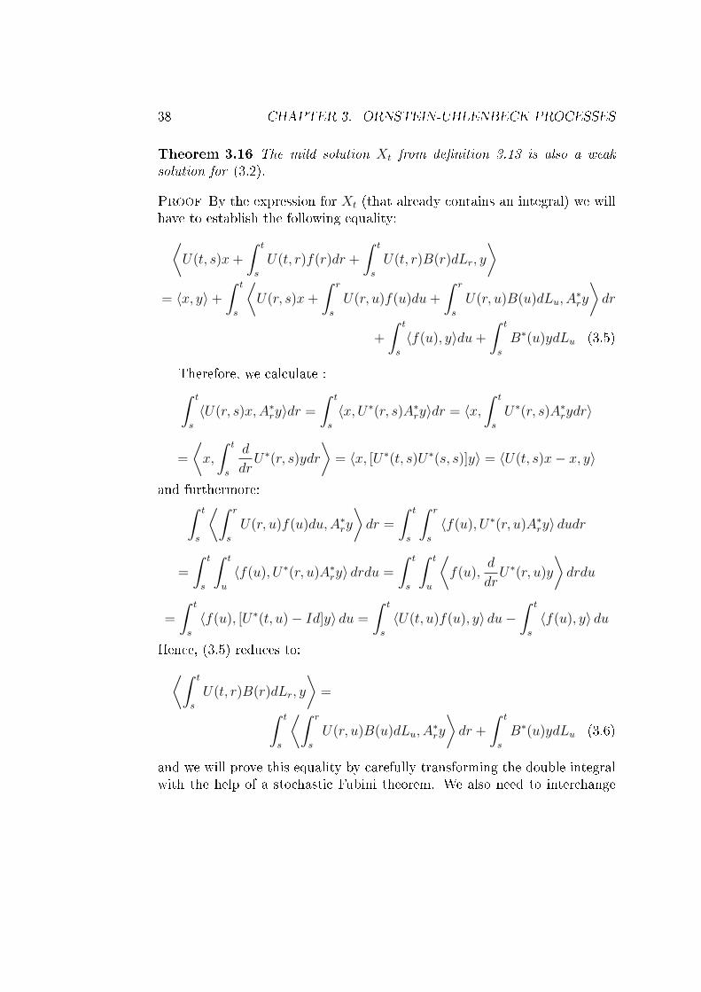
Theorem 3.16 The mild solution Xt from denition 3.13 is also a weaksolution for (3.2).
Proof By the expression for Xt (that already contains an integral) we willhave to establish the following equality:⟨
U(t, s)x +
∫ t
s
U(t, r)f(r)dr +
∫ t
s
U(t, r)B(r)dLr, y
⟩= 〈x, y〉+
∫ t
s
⟨U(r, s)x +
∫ r
s
U(r, u)f(u)du +
∫ r
s
U(r, u)B(u)dLu, A∗ry
⟩dr
+
∫ t
s
〈f(u), y〉du +
∫ t
s
B∗(u)ydLu (3.5)
Therefore, we calculate :∫ t
s
〈U(r, s)x, A∗ry〉dr =
∫ t
s
〈x, U∗(r, s)A∗ry〉dr = 〈x,
∫ t
s
U∗(r, s)A∗rydr〉
=
⟨x,
∫ t
s
d
drU∗(r, s)ydr
⟩= 〈x, [U∗(t, s)U∗(s, s)]y〉 = 〈U(t, s)x− x, y〉
and furthermore:∫ t
s
⟨∫ r
s
U(r, u)f(u)du, A∗ry
⟩dr =
∫ t
s
∫ r
s
〈f(u), U∗(r, u)A∗ry〉 dudr
=
∫ t
s
∫ t
u
〈f(u), U∗(r, u)A∗ry〉 drdu =
∫ t
s
∫ t
u
⟨f(u),
d
drU∗(r, u)y
⟩drdu
=
∫ t
s
〈f(u), [U∗(t, u)− Id]y〉 du =
∫ t
s
〈U(t, u)f(u), y〉 du−∫ t
s
〈f(u), y〉 du
Hence, (3.5) reduces to:⟨∫ t
s
U(t, r)B(r)dLr, y
⟩=∫ t
s
⟨∫ r
s
U(r, u)B(u)dLu, A∗ry
⟩dr +
∫ t
s
B∗(u)ydLu (3.6)
and we will prove this equality by carefully transforming the double integralwith the help of a stochastic Fubini theorem. We also need to interchange

3.4. EXISTENCE OF THE WEAK SOLUTION 39
scalar product and the stochastic integral in some respect, requiring a lemmaintroduced in [App06]. As the Hilbert space valued integral there was calledstrong stochastic integral and the real valued version was called weak stochas-tic integral, the ability to interchange scalar product and integral was referedto as weak-strong-compatibility. We shortly cite both results giving only theidea of the proof.
Proposition 3.17 (stochastic Fubini) Let be (M,M, µ) a measure spacewith µ nite. By G2(M) denote the space of all L(H, H ′)- valued mappingsR on [s, t] ×M such that (r, m) 7→ R(r, m)y is measurable for each y ∈ H
and ‖R‖2G2(M) :=
∫ t
s
∫M‖R(r, m)T
12
x ‖2ν(dx)µ(dm)dr < ∞ Then we have:
∫M
(∫ t
s
R(u, m)dLu
)µ(dm) =
∫ t
s
(∫M
R(u, m)µ(dm)
)dLu
Proof see [Stolze05] Theorem 3.3.4The idea is simply (after verifying that both sides make sense) to check theequality on simple functions dense in G2(M) and then to extend it to thewhole space.
Lemma 3.18 (weak-strong-compatibility) Let be R ∈ H2 and y ∈ H.Then we have: ⟨∫ t
s
R(r)dLr, y
⟩=
∫ t
s
R∗(r)ydLr
Proof see [Stolze05] Again, the idea is to assure that both sides are welldened, then to check the equality on simple functions and to extend it toall of H2.
Remark 3.19 In [Stolze05] the last two results are formulated only for theintegral with respect to the martingale measure. Of course the general resultsinvolve nothing more than the stochastic Fubini theorem for Wiener integrals,the ordinary Fubini theorem and, for the weak-strong compatibility, the abilityto interchange bounded linear operators with Bochner integrals.

40 CHAPTER 3. ORNSTEIN-UHLENBECK PROCESSES
Now we are able to nish our proof of 3.16:∫ t
s
⟨∫ r
s
U(r, u)B(u)dLu, A∗ry
⟩dr
=
∫ t
s
(∫ r
s
B∗(u)U∗(r, u)A∗ry dLu
)dr by weak-strong-compatibility
=
∫ t
s
(∫ t
u
B∗(u)U∗(r, u)A∗ry dr
)dLu by stochastic Fubini
=
∫ t
s
(B∗(u)
∫ t
u
d
drU∗(r, u)y dr
)dLu
=
∫ t
s
B∗(u)[U∗(t, u)− Id]y dLu
=
⟨∫ t
s
[U(t, u)− Id]B(u)dLu, y
⟩by weak-strong-compatibility
=
⟨∫ t
s
U(t, u)B(u)dLu, y
⟩−⟨∫ t
s
B(u)dLu, y
⟩
and that is precisely what we had to show.

Chapter 4
Semigroup and Invariant Measure
Now that we have solved our equation, we turn our interest to the associatedsemigroup. Since the coecients are time-dependent, this semigroup willdepend on two parameters. This leads us to a generalization of invariantmeasures for two-parameter semigroups - an evolution system of measures,dened in section 4.2.
The proof of our rst main theorem - concerning existence and uniquenessof such an evolution system of measures - is already quite demanding, so wehave collected some necessary prerequisites in section 4.1. Here we startby deriving the characteristic function of our solution, using our results onstochastic convolution from the preceding chapter. The Fourier transformof the solution will be a valuable tool throughout the rest of this thesis.As another helpful lemma, we provide a slightly extended monotone classtheorem. With its help, we establish the required ow property to assurethat we are dealing indeed with a semigroup.
Then in section 4.3 we investigate the respective autonomous equation,obtained by articially enlarging the state space. The reason for this lies inour interest in generators of semigroups. Alas, for two-parameter semigroups,no sensible concept for generators is known, thus we have to introduce aone-parameter semigroup that incorporates all the information of the two-parameter semigroup.
Having done so, we are able to establish existence and uniqueness of aninvariant measure for this new semigroup, where the invariant measure isbasically given by dt⊗ νt where νt is the evolution system of measures fromsection 4.2. In order to obtain a probability measure, it is crucial to haveT -periodicity of the νt, so that instead of dt we may consider dt restricted
41

42 CHAPTER 4. SEMIGROUP AND INVARIANT MEASURE
to [0, T ] which we can normalize. Moreover, we prove that the semigroup onthe respective L2-space is a contraction.
Next we turn to the innitesimal generator of our semigroup. Our rstresult states that the semigroup is indeed strongly continuous on the L2-space, that is, it fullls a condition assuring the existence of a generator ona dense subspace. Next we identify a dense subspace of test functions thatcontains all the information about the generator. In semigroup theory, sucha subspace is called a core. On this core, the generator is seen to be the sumof a dierential operator and a nonlocal operator given by a superposition ofdierence operators. Moreover, we obtain some information on the spectrumof the generator.
In section 4.4 we prove two functional inequalities related to our semi-group. We will phrase the results both in terms of the one-parameter andof the two-parameter semigroup. A central tool - the so-called square eldoperator - is introduced in subsection 4.4.1. We calculate its precise formand establish an important inequality, relating the square eld operator andthe semigroup. Then we deduce a Poincaré and a Harnack inequality.
Beware of a change in notation, in this chapter the Lévy triple associated toL will be denoted by [b, R, m]. Moreover, as a technical assumption that willbe necessary for proposition 4.19, we will require the coecients in (3.2) tobe T-periodic for some T > 0.
Assumption 4.1 From now on, we assume that there exists T >0 such thatthe coecients A, f and B in (3.2) are T -periodic.
4.1 Preliminaries
Recall that the weak solution for (3.2) takes the following form:
X(t, s, x) = U(t, s)x +
∫ t
s
U(t, r)f(r)dr +
∫ t
s
U(t, r)B(r)dLr
As opposed to the Gaussian case we are no longer able to give an easyrepresentation of the law of X(t, s, x), but we can calculate its Fourier trans-form:

4.1. PRELIMINARIES 43
Lemma 4.2 (characteristic function)
E [exp (i 〈h,X(t, s, x)〉)] =
exp
i
⟨h, U(t, s)x +
∫ t
s
U(t, r)f(r)dr
⟩exp
∫ t
s
λ(B∗(r)U∗(t, r)h)dr
where λ is the Lévy symbol of L.
Proof : Knowing how the Fourier transform acts on translations, it will beenough to show, that:
E[exp
(i
⟨h,
∫ t
s
U(t, r)B(r)dLr
⟩)]= exp
∫ t
s
λ(B∗(r)U∗(t, r)h)dr
Using the results from the last chapter, the continuity of U and B allowsus to approximate the Lévy stochstic integral by a sequence of sums. Moreprecisely, we want to prove the claim:∫ t
s
U(t, r)B(r)dLr = P − limn→∞
∑si∈Pn
U(t, si)B(si)(Lsi− Ls(i−1)∨0
)
where the limit is taken in probability and Pn is a sequence of partitionss = s0 < ... < sN = t of [s, t] such that the mesh width tends to zero. Asthe Lévy stochastic integral is composed of four dierent terms (see (3.1))we will show this equality separately for each of them.
We will need r 7→ U(t, r) B(r) to be strongly continuous and this is thecase, since the composition of strongly continuous bounded operators is againstrongly continuous:
‖Ut(r)B(r)x− Ut(s)B(s)x‖≤ ‖Ut(r)B(r)x− Ut(s)B(r)x‖+ ‖Ut(s)B(r)x− Ut(s)B(s)x‖
≤ ‖[Ut(r)− Ut(s)]B(r)x‖+ ‖Ut(s)‖L(H)‖B(r)−B(s)x‖s→t
−→ 0
where both terms tend to zero because of strong continuity.
For the drift term which is a Bochner integral we have to show that:
limn→∞
∑si∈Pn
∫ si
si−1
‖U(t, si)B(si)b− U(t, r)B(r)b‖ dr = 0

44 CHAPTER 4. SEMIGROUP AND INVARIANT MEASURE
but since r 7→ Ut(r)B(r)b is even uniformly continuous on [s, t] we may ndδ > 0 such that ‖Ut(r)B(r)b− Ut(r
′)B(r′)b‖ < εt−s
whenever |r − r′| < δ, sothat if we choose n such that the mesh width of Pn is smaller than δ we have∑
si∈Pn
∫ si
si−1
‖U(t, si)B(si)b− U(t, r)B(r)b‖ dr <∑
si∈Pn
∫ si
si−1
ε
t− sdr < ε
For the small jumps we make use of the isometry from 3.7, so we have toshow that our piecewise approximation converges in the H2 norm, that is weneed:
limn→∞
∞∑k=1
∫‖x‖<1
(∑si∈Pn
∫ si
si−1
‖[Ut(r)B(r)− Ut(si)B(si)]T12
x ek‖2dr
)M(dx) = 0
For each k and x xed the expression in round brackets converges to zero,for the same reasons as used for the drift term. So we only have to showthat we may take the limit into the sum and the integral, but this follows bydominated convergence on considering the uniform integrable bound :
‖[Ut(r)B(r)−Ut(si)B(si)]T12
x ek‖2 ≤ 2 sups≤r≤t
‖Ut(r)‖L(H) sups≤r≤t
‖B(r)‖L(H)‖T12
x ek‖2
Thus we have convergence in L2 of the approximating sums towards theintegral.The same argument works for the Brownian part, where there is even nodependence on x.The big jumps, nally are quite simple to treat. Since the expression makessense pointwise, we consider the approximation for ω xed and we obtain:
limn→∞
∑si∈Pn
∑si−1≤r≤si
[Ut(si)B(si)− Ut(r)B(r)]∆Lr(ω)χ‖∆Lr(ω)‖>1 = 0
again because of strong continuity.So in any of the four cases we have at least convergence in probability
and the claim is proved.Since convergence in probability implies convergence in distribution and
x 7→ ei〈h,x〉 is bounded and continuous, we may interchange limit and expec-tation:
E[exp
(i
⟨h,
∫ t
s
U(t, r)B(r)dLr
⟩)]

4.1. PRELIMINARIES 45
= limn→∞
E
[exp
(i
⟨h,∑k∈Pn
U(t, sk)B(sk)(Lsk− Lsk−1∨0)
⟩)]Using the functional equation of the exponential and the independence ofincrements of L:
= limn→∞
∏k∈Pn
E[exp
(i⟨h, U(t, sk)B(sk)(Lsk
− Lsk−1∨0)⟩)]
= limn→∞
∏k∈Pn
exp λ(B∗(sk)U∗(t, sk)h)(sk − (sk−1 ∨ 0))
= exp
∫ t
s
λ(B∗(r)U∗(t, r)h)dr
where we employed the Lévy-Khinchine formula and the functional equationagain. Note that the Riemannian sums converge to the integral because ofstrong continuity.
The following lemma will be of great technical help.
Lemma 4.3 (complex monotone classes) LetH be a complex vector spaceof complex-valued bounded functions, that contains the constants and is closedunder componentwise monotone convergence. Let M ⊂ H be closed undermultiplication and complex conjugation. Then, all bounded σ(M)- measur-able functions belong to H.
Proof Without loss of generality, we can assume that M already is analgebra, by taking its linear hull, which changes neither the multiplicativity,nor the generated σ-algebra. As M is closed under complex conjugation,we have MR := <f,=f | f ∈ M ⊂ M. As M is multiplicative, MRis a real algebra of real-valued functions. Of course, MR ⊂ HR, where HRis the monotone real vector space of real-valued elements of H. Now wecan apply the standard monotone class theorem, which states, that everybounded σ(MR)-measurable real-valued function belongs to HR ⊂ H. Toobtain our conclusion, we have to show, that σ(M) ⊂ σ(MR). The elementsof σ(M) are of the form Af := f−1(A) for a Borel-set A ∈ C and a f ∈M.IfA = B×C is a rectangle, we have Af = B<f ∩C=f . But since preimages andset operations commute, it is clear, that it is sucient to have the inclusionfor rectangles, as these form a generator for B(C). It is also obvious, thatany complex-valued function in H can be reconstructed from its real andimaginary parts.

46 CHAPTER 4. SEMIGROUP AND INVARIANT MEASURE
The last and the next result in combination will be particularly useful:
Lemma 4.4 The functions M := ei〈h,x〉, h ∈ H form a complex multi-plicative systems that generates the Borel σ-algebra of H.
Proof It is obvious that M is closed under multiplication and complexconjugation.To show that indeed σ(M) = B(H) we make use of the following lemma:(see [Schw73] page 108)
Lemma 4.5 A countable family of real-valued functions on a Polish spaceX separating the points of X already generates the Borel-sigma-algebra of X.
Our countable family will be fn,k(x) := sin(〈 1nek, x〉)k,n∈N ⊂M where ek
is an orthonormal basis of H.Since the sine function is injective in a neighborhood of zero, and the func-tions 〈 1
nek, x〉) separate the points of H, so do the fn,k. As real and imaginary
parts of functions inM, it is clear, that the sigma-algebra generated by themis included in σ(M).
Now we will show that our solution induces a two-parameter semigroup,dened as follows:
Denition 4.6 Whenever f : H → C is measurable and bounded, dene
P (s, t)f(x) := E[f(X(t, s, x))]
P (s, t) will be called the two-parameter semigroup (associated to the solutionX).
Lemma 4.7 For f as above, we have the following ow property:
P (r, s)P (s, t)f(x) = P (r, t)f(x)
Proof We will show the equality for the functions fh(x) = ei〈h,x〉 and extendit with the help of 4.3. First note, that by 4.2 we have
P (s, t)fh(x) = exp i 〈h, U(t, s)x〉 exp
i
⟨h
∫ t
s
U(t, r)f(r)dr
⟩× exp
∫ t
s
λ(B∗(r)U∗(t, r)h)dr

4.2. EVOLUTION SYSTEMS OF MEASURES 47
so that:
P (r, s)P (s, t)fh(x)
= E[P (s, t)fh(X(s, r, x)]
= E [exp i 〈U∗(t, s)h,X(s, r, x)〉]× exp
i
⟨h,
∫ t
s
U(t, r)f(r)dr
⟩× exp
∫ t
s
λ(B∗(r)U∗(t, r)h)dr
but again 4.2 gives us the Fourier transform of X(s, r, x) this time evaluatedat U∗(t, s)h:
= exp i 〈U∗(t, s)h, U(s, r)x〉
× exp
i
⟨U∗(t, s)h,
∫ s
r
U(s, q)f(q)dq
⟩exp
i
⟨h,
∫ t
s
U(t, r)f(r)dr
⟩× exp
∫ s
r
λ(B∗(q)U∗(s, q)U∗(t, s)h)dq
exp
∫ t
s
λ(B∗(r)U∗(t, r)h)dr
Interchanging U(t, s) with the integral, as it is a bounded operator, makinguse of the semigroup property of U and U∗ and combining the integralsyields the result for exponential f . The space of all bounded measurable ffor which the ow property holds is a complex monotone vectorspace, sinceby monotone convergence :
P (s, t) limn→∞
fn(x) = E[ limn→∞
fn(X(s, r, x))]
= limn→∞
E[fn(X(s, r, x))] = P (s, t) limn→∞
fn(x)P (s, t)fn(x)
and by monotonicity of the integral we have even P (s, t)fn(x) P (s, t)f(x)so that we can apply monotone covergence again to obtain:
P (r, s)P (s, t) limn→∞
fn(x) = P (r, s) limn→∞
P (s, t)fn(x) = limn→∞
P (r, s)P (s, t)fn(x)
Hence, the proof is complete.
4.2 Evolution Systems of Measures
Since our equation is non-autonomous we cannot hope for a single invariantmeasure. What one can still expect in our setting is a so called evolution

48 CHAPTER 4. SEMIGROUP AND INVARIANT MEASURE
system of measures, a whole family νtt∈R of measures such that for alls < t and all bounded measurable f :∫
Rn
P (s, t)f(x)νs(dx) =
∫Rn
f(x)νt(dx) (4.1)
To assure the existence of such a system, besides assumption 3.11 we willhenceforth require the following condition to hold:
Assumption 4.8 We assume a weak regularity for the Levy symbol λ , thatis: for the corresponding Lévy measure M holds:∫
‖x‖>1
‖x‖M(dx) < ∞
Taking a clue from the Gaussian situation, we will consider the distributionof our solutions after an innite time span. As we have explicit knowledgeof the Fourier transforms, we will characterize the measures in that way.
The following lemma will give a useful growth condition for the Lévysymbol that will allow us to construct limit measures.
Lemma 4.9 Every Lévy symbol λ with a Lévy measure M satisfying 4.8 isFréchet dierentiable. In particular such a λ is locally of linear growth.
Proof : Let be λ the corresponding Lévy symbol and M the Lévy measure.By the Lévy-Khinchine formula 2.36 we know that:
λ(u) = i〈u, b〉 − 1
2〈u, Au〉+
∫ (ei〈u,x〉 − 1− i〈u, x〉χ‖x‖≤1
)M(dx)
Clearly, it is enough to show that the integral expression is dierentiable.We rst show Gâteaux dierentiability, hence we will need the directionalderivatives to be integrable to obtain the result via dominated convergence.We have:
∂
∂t
∣∣∣∣t=0
(ei〈u+tv,x〉 − 1− i〈u + tv, x〉χ‖x‖≤1
)= i〈v, x〉ei〈u,x〉 − i〈v, x〉χ‖x‖≤1

4.2. EVOLUTION SYSTEMS OF MEASURES 49
To see the integrability we split the integral in two parts:∫‖x‖≤1
∣∣i〈v, x〉ei〈u,x〉 − i〈v, x〉χ‖x‖≤1∣∣M(dx)
=
∫‖x‖≤1
∣∣∣∣∣i〈v, x〉∞∑
k=0
(i〈u, x〉)k
k!− i〈v, x〉
∣∣∣∣∣M(dx)
≤∫‖x‖≤1
(‖v‖ ‖x‖
∞∑k=1
|(i〈u, x〉)|k
k!
)M(dx)
≤∫‖x‖≤1
(‖v‖ ‖x‖
∞∑k=1
‖u‖k‖x‖k
k!
)M(dx)
≤∫‖x‖≤1
(‖v‖ ‖x‖2‖u‖
∞∑k=1
‖u‖k−1‖x‖k−1
k!
)M(dx)
≤ sup‖x‖≤1
exp‖u‖‖x‖∫‖x‖≤1
(‖v‖ ‖x‖2‖u‖
)M(dx)
= exp‖u‖‖u‖ ‖v‖∫‖x‖≤1
‖x‖2M(dx) < ∞
for every xed u, v and s since M is a Lévy measure. On the other hand,we have:∫
‖x‖>1
∣∣i〈v, x〉ei〈u,x〉 − i〈v, x〉χ‖x‖≤1∣∣M(dx) ≤ ‖v‖
∫‖x‖>1
‖x‖M(dx) < ∞
by assumption.Moreover, from the above, it is easy to see that the Gâteaux derivative is lin-ear and bounded and depends continuously on u with respect to the operatornorm, so λ is Fréchet dierentiable and hence locally Lipschitz.
Theorem 4.10 Assume hypothesis 4.8. Then the functions
νt(h) := exp
i
⟨h,
∫ t
−∞U(t, r)f(r)dr
⟩exp
∫ t
−∞λB∗(r)U∗(t, r)hdr
are the Fourier transforms of an evolution system of measures.This system is T -periodic, that is we have νT+t = νt for any t.Any other T -periodic evolution system of measures, coincides with the above.

50 CHAPTER 4. SEMIGROUP AND INVARIANT MEASURE
Proof : To establish T -periodicity, rst note, that we have:U(t, s) = U(t + T, s + T ) for any s < t, which follows easily from its deningdierential equation and the assumption that A is T -periodic. Hence, we get∫ t+T
−∞U(t+T, r)f(r)dr =
∫ t
−∞U(t+T, r+T )f(r+T )dr =
∫ t
−∞U(t, r)f(r)dr
and for the other integral the argument is the same.We have to assure that the integrals above exist. Since U is stable and f
is bounded on all of R (as it is continuous and periodic) we have:∫ t
−∞‖U(t, r)f(r)‖dr ≤
∫ t
−∞Me−ω(t−r)‖f‖∞dr =
M
ω‖f‖∞
As λ is Fréchet dierentiable it has locally linear growth, so that withλ(0) = 0 we have ‖λ(u)‖ ≤ C‖u‖ on the bounded range of the argument forsome C > 0. So with ‖B∗‖ bounded we can treat the second integral as therst:
∫ t
−∞‖λB∗(r)U∗(t, r)h‖dr ≤ C
∫ t
−∞‖B∗(r)U∗(t, r)h‖dr
≤ C supr‖B∗(r)‖M
ω‖h‖ < ∞ (4.2)
where we have used, that ‖U∗‖ = ‖U‖.
To show that these functions are indeed Fourier transforms of measures wecan make use of Lévy's continuity theorem in the nite dimensional case.We have just proven pointwise convergence of the Fourier transforms of P [X(t, s, x)]−1, and that the limit function is continuous in 0 follows easily bydominated convergence. Pointwise convergence under the integral is clear bycontinuity of λ, U and B and a majorizing function is found by looking at(4.2) again.In the innite dimensional case, however, we cannot apply Lévy's continuitytheorem for reasons explained in appendix B. For a better readability wepostpone the somewhat technical alternative.
In order to see that the respective measures constitute an evolution system

4.2. EVOLUTION SYSTEMS OF MEASURES 51
of measures we will check (4.1) for exponential functions and then extendthe result via monotone classes.So if we take k(x) = ei〈h,x〉 in (4.1) we get:∫
Rn
k(x)νt(dx) = νt(h)
by the very denition of Fourier transformation.On the other hand we have by 4.2:
P (s, t)k(x) =
ei〈h,U(t,s)x〉 exp
i
⟨h,
∫ t
s
U(t, r)f(r)dr
⟩exp
∫ t
s
λB∗(r)U∗(t, r)hdr
Using the adjoint of U and the fact that Fourier transformation is only withrespect to x we obtain by denition of νs:∫
Rn
P (s, t)k(x)νs(dx)
= νs(U∗(t, s)h) exp
i
⟨h,
∫ t
s
U(t, r)f(r)dr
⟩+
∫ t
s
λB∗(r)U∗(t, r)hdr
= exp
i
⟨U∗(t, s)h,
∫ s
−∞U(s, r)f(r)dr
⟩+
∫ s
−∞λB∗(r)U∗(s, r)U∗(t, s)hdr
exp
i
⟨h,
∫ t
s
U(t, r)f(r)dr
⟩+
∫ t
s
λB∗(r)U∗(t, r)hdr
= exp
i
⟨h,
∫ s
−∞U(t, s)U(s, r)f(r)dr
⟩+
∫ s
−∞λB∗(r)U∗(t, r)hdr
exp
i
⟨h,
∫ t
s
U(t, r)f(r)dr
⟩+
∫ t
s
λB∗(r)U∗(t, r)hdr
where we used in the left part, that linear continuous operators commute withthe integral, and in the right part the corresponding ("twisted") semigroupproperty for the adjoints.
= exp
i
⟨h,
∫ s
−∞U(t, r)f(r)dr
⟩+ i
⟨h,
∫ t
s
U(t, r)f(r)dr
⟩exp
∫ s
−∞λB∗(r)U∗(t, r)hdr +
∫ t
s
λB∗(r)U∗(t, r)hdr

52 CHAPTER 4. SEMIGROUP AND INVARIANT MEASURE
= exp
i
⟨h,
∫ t
−∞U(t, r)f(r)dr
⟩exp
∫ t
−∞λB∗(r)U∗(t, r)hdr
but the last line equals νt(h) and that is precisely what we had to show.
To prove the full assertion we have to show that (4.1) not only holdsfor functions of the form kh(x) := ei〈h,x〉, but for any bounded measurablefunction.By 4.4 we can apply 4.3, because the bounded and measurable functions forwhich (4.1) holds, form a complex monotone vector space:for constant functions the equality is trivial and that (4.1) holds for monotonelimits is essentially an iterated application of Levy's theorem about monotoneconvergence. Hence, all bounded measurable functions satisfy (4.1) and theexistence of an evolution system of measures is proved.
To prove uniqueness, let νs be another T -periodic family satisfying (4.1),then it follows by periodicity:
νs(h) = νs(U∗(s + T, s)h)
×exp
i
⟨h,
∫ s+T
s
U(s + T, r)f(r)dr
⟩+
∫ s+T
s
λB∗(r)U∗(s + T, r)hdr
Using the easy to check relations:
∫ s+T
s
U(s+T, r)f(r)dr =
∫ s
−∞U(s, r)f(r)dr−U(s+T, s)
∫ s
−∞U(s, r)f(r)dr
∫ s+T
s
λB∗(r)U∗(s + T, r)hdr =∫ s
−∞λB∗(r)U∗(s, r)hdr −
∫ s
−∞λB∗(r)U∗(s + T, r)hdr

4.2. EVOLUTION SYSTEMS OF MEASURES 53
we get:
νs(h) = νs(U∗(s + T, s)h) exp
i
⟨h,
∫ s
−∞U(s, r)f(r)dr
⟩exp
∫ s
−∞λB∗(r)U∗(s, r)hdr
exp
i
⟨h,−U(s + T, s)
∫ s
−∞U(s, r)f(r)dr
⟩exp
−∫ s
−∞λB∗(r)U∗(s + T, r)hdr
or equivalently:
νs(h)
[exp
i
⟨h,
∫ s
−∞U(s, r)f(r)dr
⟩exp
∫ s
−∞λB∗(r)U∗(s, r)hdr
]−1
= νs(U∗(s + T, s)h)
[exp
i
⟨U∗(s + T, s)h,
∫ s
−∞U(s, r)f(r)dr
⟩exp
∫ s
−∞λB∗(r)U∗(s + T, r)hdr
]−1
Finding, that the second line is the rst, with h replaced by U∗(s+T, r)h wecan iterate, since the relation was valid for all h ∈ H. As ‖U∗(s + T, r)‖ < 1must hold by our stability assumption, all the factors in the second equationwill tend to 1, so νs must indeed have the desired form.
Remark 4.11 The condition that the Lévy symbol is of linear growth is ac-tually stronger than necessary. To assure the existence of the integral in(4.2) it would be even sucient to have a very weak estimate of the form|λ(u)| = O(
√‖u‖). But we were unable to nd any other easy to check con-
ditions to control the growth of a Lévy symbol around the origin. Moreover,in the innite dimensional case, we make full use of our assumption, as canbe seen next.
Proof (νt is a characteristic function - Hilbert space case)The general idea is the following. In the Gaussian case, it is known thatthe limit distributions are Gaussian again. In the same manner we takeadvantage of the fact that, in the Lévy case, our limit distribution is innitely

54 CHAPTER 4. SEMIGROUP AND INVARIANT MEASURE
divisible. We proceed here as in [Fuhr/Röck00] chapter 3. First of all weshow that our distributions P X(t, s, x) are innitely divisible for any t >s, x. By the Lévy-Khinchine representation it is sucient to prove thattheir characteristic functions have the form (2.5) for some triple [b, Q, M ].Therefore, we calculate:
exp
∫ t
s
λ(B∗rU
∗t,rh)dr
= exp
∫ t
s
i〈b, B∗rU
∗t,rh〉dr − 1
2
∫ t
s
〈B∗rU
∗t,rh,RB∗
rU∗t,rh〉dr
+
∫ t
s
(∫H
ei〈x,B∗r U∗t,rh〉 − 1− i〈x, B∗rU
∗t,rh〉χ‖x‖≤1M(dx)
)dr
For the jump part we have:
∫H
ei〈x,B∗r U∗t,rh〉 − 1− i〈x, B∗rU
∗t,rh〉χ‖x‖≤1M(dx)
=
∫H
ei〈Ut,rBrx,h〉 − 1− i〈Ut,rBrx, h〉χ‖x‖≤1M(dx)
+
∫H
[−χ‖Ut,rBrx‖≤1 + χ‖Ut,rBrx‖≤1]M(dx)
=
∫H
ei〈x,h〉 − 1− i〈x, h〉χ‖x‖≤1M (Ut,rBr)−1(dx) (4.3)
−∫
H
i〈Ut,rBrx, h〉[χ‖x‖≤1 − χ‖Ut,rBrx‖≤1]M(dx) (4.4)
Note that (4.3) is nite because of: (setting C := ‖Ut,rBr‖L(H))
∫H
(1 ∧ ‖x‖2)M (Ut,rBr)−1(dx) =
∫H
(1 ∧ ‖Ut,rBrx‖2)M(dx)
≤∫
H
(1 ∧ C2‖x‖2)M(dx) ≤ C2
∫H
(1
C2∧ ‖x‖2)M(dx) < ∞
and only in that way we can argue that (4.4) must be nite as well. Thus,

4.2. EVOLUTION SYSTEMS OF MEASURES 55
we obtain:
exp
∫ t
s
λ(B∗rU
∗t,rh)dr
= exp
i
⟨∫ t
s
Ut,rBrb dr, h
⟩− 1
2
⟨h,
∫ t
s
Ut,rBrRB∗rU
∗t,rhdr
⟩+
∫ t
s
(∫H
ei〈x,h〉 − 1− i〈x, h〉χ‖x‖≤1M (Ut,rBr)−1(dx)
)dr
− i
⟨∫ t
s
∫H
Ut,rBrx[χ‖x‖≤1 − χ‖Ut,rBrx‖≤1]M(dx)dr, h
⟩so that with:
• b(t, s) :=∫ t
sUt,rBrbdr−
∫ t
s
∫H
Ut,rBrx[χ‖x‖≤1−χ‖Ut,rBrx‖≤1]M(dx)dr
• Q(t, s) :=∫ t
sUt,rBrRB∗
rU∗t,rdr
• Mt,s(A) :=∫ t
sM (Ut,rBr)
−1(A)dr for 0 /∈ A
exp∫ t
sλ(B∗
rU∗t,rh)dr
is associated to the triple [b(t, s), Q(t, s), Mt,s], where
Q(t, s) is still symmetric and nonnegative and we have :
trQ(t, s) =∑
k
〈ek, Q(t, s)ek〉 =∑
k
∫ t
s
‖√
RB∗rU
∗t,rek‖2
=
∫ t
s
‖√
RB∗rU
∗t,r‖2
2 ≤∫ t
s
‖√
R‖22‖B∗
rU∗t,r‖2 < ∞
and Mt,s is a Lévy measure, as we have [since (1∧ ‖x‖2) ≤ (‖x‖ ∧ ‖x‖2)]:∫ t
s
∫H
(1 ∧ ‖x‖2)M (Ut,rBr)−1(dx) ≤
∫ t
s
∫H
(‖x‖ ∧ ‖x‖2)M (Ut,rBr)−1(dx)
=
∫ t
s
∫H
(‖Ut,rBrx‖ ∧ ‖Ut,rBrx‖2)M(dx)
≤∫ t
s
‖Ut,rBr‖∫
H
(‖x‖ ∧ ‖Ut,rBr‖ ‖x‖2)M(dx)
≤∫ t
s
maxr≤t
‖Br‖Me−ω(t−r)
∫H
(‖x‖ ∧maxr≤t
‖Ut,rBr‖ ‖x‖2)M(dx)︸ ︷︷ ︸<∞ by assumption 4.8
< ∞

56 CHAPTER 4. SEMIGROUP AND INVARIANT MEASURE
Moreover, we see that we can let s → −∞ and Q(t,−∞) will still be traceclass as well as Mt,−∞ will still be a Lévy measure, because of the exponentialstability of U . Since we already know that the Fourier transform as a wholeconverges, convergence of the rst part of b(t,−∞) (which is obvious) impliesconvergence of the second part. Hence the limit function is associated toa Lévy triple and thus the characteristic function of an innitely divisiblemeasure.
Remark 4.12 Note that we did not show weak convergence and that we donot need to do so. The point is only in proving that our limit functionsare indeed associated to measures. Extension to functions more general thancomplex exponentials is then done by monotone class arguments.

4.3. THE REDUCED EQUATION 57
4.3 The Reduced Equation
Since we are interested in generators, we have to reduce our equation tothe autonomous case, so that we obtain a one-parameter semigroup, thatwe can relate to a generator. It will turn out, that we can establish aninvariant measure for our new semigroup on the extended state space, usingour evolution system of measures.
Reduction of non-autonomous problems is a well-known method in thetheory of ordinary dierential equations.(see e.g. [Dal/Krei74]) We recallthat the basic idea is to enlarge the state space, thus allowing to keep trackof the elapsed time. The reduced problem then looks:
dX(t) = A(y(t))X(t) + f(y(t))dt + B(y(t))dL(t) X(0) = x
dy(t) = dt y(0) = s
The one-parameter semigroup is then dened as follows:
Pτu(t, x) := Pt,t+τu(t + τ, ·)(x) := (Pt,t+τut+τ )(x)
meaning that we apply the two-parameter semigroup to u as a function ofx only. That the family Pττ∈R is indeed a semigroup, follows, of course,from the semigroup property of Ps,ts<t and is a simple calculation:
(Pσ(Pτu))(t, x) = Pt,t+σPt+σ,t+σ+τu(t + σ + τ, ·)(x)
= Pt,t+σ+τu(t + σ + τ, ·)(x) = Pτ+σu(t, x)
4.3.1 The Invariant Measure ν and the Space L2∗(ν)
Starting from our evolution system of measures, we will establish an invariantmeasure for the one-parameter semigroup. On the respective L2-space thesemigroup will then be a contraction.
From now on we will require the following assumption to hold:
Assumption 4.13 D(A∗) is dense in H and we have U∗(t, s)D(A∗) ⊂ D(A∗)for all s ≤ t. Moreover, we have d
dtU∗(t, s)x = U∗(t, s)A∗(t)x for all x ∈
D(A∗)
To obtain our invariant measure we need the following lemma:
Lemma 4.14 The function F : (t, A) 7→ νt(A) is a transition kernel.

58 CHAPTER 4. SEMIGROUP AND INVARIANT MEASURE
Proof Obviously, for xed t we have a measure.To show measurability, we will need a monotone class argument:H := f : H → C | t 7→
∫f(x)νt(dx) is measurable is a monotone
complex vector space, since pointwise limits of measurable functions are againmeasurable.M := exp(〈h, x〉)h∈H is a complex multiplicative system, suchthat σ(M) = B(H) (see 4.5 and the following arguments)We will have proved the lemma, once we know that M⊂ H.Therefore, we will show that t 7→
∫f(x)νt(dx) is even continuous for all
f ∈MRecalling the form of the Fourier transforms,
νt(h) = exp
i
⟨h,
∫ t
−∞U(t, r)f(r)dr
⟩exp
∫ t
−∞λB∗(r)U∗(t, r)hdr
it will be sucient to show that:∫
Rχr≤sλB∗(r)U∗(s, r)hdr
s→t−→∫ t
−∞λB∗(r)U∗(t, r)hdr
Pointwise convergence of the integrands is clear, and an integrable upperbound is given by: C χr≤smax M e−ω(smin−r)
where C is composed of the Lipschitz constant of λ and a bound for ‖B(r)‖and smin, smax are upper and lower bounds for the convergent sequence sn,while M and ω are the stability constants for U .The argument for the other integral follows the same lines.
Now, we introduce the space, on which the semigroup will be strongly con-tinuous and the subspace that will be the core for the generator of our semi-group. Let be
Denition 4.15 As F is a kernel from H to R we can form ν := F ⊗ 1Tdt,
a measure on H × R.
L2∗(ν) :=f : R×H → R measurable | f(t + T, x) = f(t, x) ν − a.e.∫
[0,T ]×H
‖f‖2(y)ν(dy) < ∞

4.3. THE REDUCED EQUATION 59
M := spanCf : R×H → C | f = Φ(t)ei〈x,h(t)〉, where
Φ ∈ C1(R, R) and T-periodic,
h ∈ C1(R, H) and T-periodic such that Im h ⊂ D(A∗)
K := <(f) | f ∈MThat is, K comprises the real parts of the functions in M.
Remark 4.16 L2∗ is a Hilbert space. Because of the periodicity it is clear,
that (∫
[0,T ]×H‖f‖2(y)ν(dy))
12 is a norm(where we introduce ν a.e.-equivalence
classes as usual). Given a Cauchy-sequence fn we consider f zn the restriction
of fn to the interval Iz := [zT, (z + 1)T ], z ∈ Z. By Riesz-Fischer we obtaina limit f 0 of f 0
n on [0, T ], and because of periodicity it is clear that the otherrestrictions form the same Cauchy sequences, that is: lim f z
n = f z = f 0 ∀z ∈Z. Hence, the limit function is periodic, and the space is complete.
Lemma 4.17 K is dense in L2∗(ν).
Proof Note that by periodicity, we can think of our functions to be denedon [0, T ]×H and in the following we will do so without changing notation.We will show density ofM in L2
∗(ν; C). This implies density of the respectivereal vector spaces. We will use complex monotone classes again. The spaceM is closed under multiplication and conjugation. Consider H := M as asubspace of L2
∗(ν; C) where we allow complex-valued integrable and periodicfunctions. H is a complex monotone vector space, by monotone convergence,applied separately to real and imaginary parts. So, H contains all σ(M)-measurable functons. If we can show that σ(M) = B(H × R), then we willhave all step functions in H, so density will be obvious. Note that we wantto show, that functions of the form Φi ⊗ eh generate a product σ-algebraB([0, T ])⊗ B(H). Since both families contain the constant function, we canbreak the problem down, as (1R ⊗ f)−1(A) = R× f−1(A) and knowing thatΦi generates B(R) and eh := ei〈 · ,h〉 generates B(H) (which follows again from4.5 and the fact that D(A∗) is dense), we have the result.
Remark 4.18 Note that to prove the density of K, h ≡ const is sucient,but we will need the t-dependence of h later to show that K is Pτ -invariant.
Proposition 4.19 The measure ν is the unique invariant measure for thesemigroup Pτ on L2
∗(ν). The semigroup Pτ is a contraction on L2∗(ν).

60 CHAPTER 4. SEMIGROUP AND INVARIANT MEASURE
Proof We will prove both invariance and contractivity for functions fromK rst. Since K is dense, it is then easy to see that they hold on the wholeof L2
∗(ν). Note, however, that we rst need invariance to prove contractivity,then extend contractivity by density, and then obtain global invariance bydensity and contractivity. For invariance we have to show:∫
[0,T ]×H
Pτu(t, x)dν =
∫[0,T ]×H
u(t, x)dν ∀τ > 0, u ∈ K
Writing ut(x) := u(t, x), remember, that (Pτu)(t, x) = (Pt,t+τut+τ )(x). Tak-ing into account (4.1),which is valid, since the elements from K are bounded,we have: ∫
[0,T ]×H
Pτu(t, x)dν =1
T
∫[0,T ]
∫H
(Pt,t+τut+τ )(x)νt(dx)dt
=1
T
∫[0,T ]
∫H
ut+τ (x)νt+τ (dx)dt =1
T
∫[τ,T+τ ]
∫H
ut(x)νt(dx)
=1
T
∫[0,T ]
∫H
ut(x)νt(dx) =
∫[0,T ]×H
u(t, x)dν
because of translation invariance of dt and T -periodicity of u and νt.For the contraction property we have to show: ‖Pτu‖L2
∗ ≤ ‖u‖L2∗
Using the Jensen inequality for the expectation and afterwards the invarianceproperty for u2 (recall that K is closed under multiplication):
‖Pτu‖L2∗ =
∫[0,T ]×H
E[u(t + τ,X(t + τ, t, x))]2ν(dx, dt)
≤∫
[0,T ]×H
E[u2(t + τ,X(t + τ, t, x))]ν(dx, dt) =
∫[0,T ]×H
(Pτu2)(t, x)ν(dx, dt)
=
∫[0,T ]×H
u2(t, x)ν(dx, dt) = ‖u‖L2∗
To show uniqueness, let µ be another invariant measure for Pτ , so thatwe have:∫
[0,T ]×H
Pτu(t, x)µ(dx, dt) =
∫[0,T ]×H
u(t, x)µ(dx, dt) ∀τ > 0, u ∈ L2∗(ν)
(4.5)

4.3. THE REDUCED EQUATION 61
By [Dudley89] : corollary 10.2.8 , we can disintegrate µ as follows:∫u(t, x)µ(dt, dx) =
∫[0,T ]
(∫H
u(t, x)µt(dx)
)µ1(dt) (4.6)
for the marginal µ1(dt) = µ Pr−1 where Pr is the Projection on the t-component, and µtt∈R is a family of probability measures on H. Choosingu(t, x) = f(t) independent of x in (4.5) we have by (4.6):∫
[0,T ]×H
f(t + τ)µ1(dt) =
∫[0,T ]×H
f(t)µ1(dt)
Since f is T -periodic, µ1 is translation invariant (note, that we need herea similar monotone class argument as in 4.17). So µ1 must be Lebesguemeasure.
To show µt = νt, we will of course use the uniqueness property from 4.10.Choosing u(t, x) = f(t)g(x) and τ = T in (4.5) yields:∫
[0,T ]
f(t)
(∫H
Pt,t+T g(x)µt(dx)
)µ1(dt) =
∫[0,T ]
f(t)
(∫H
g(x)µt(dx)
)µ1(dt)
Clearly, if this holds for a xed, bounded g and arbitrary bounded f , wemust have ∫
H
Pt,t+T g(x)µt(dx) =
∫H
g(x)µt(dx)
Since this holds for any bounded measurable g we can apply 4.10to obtain νt = µt ∀ t ∈ R.
Remark 4.20 Note that we cannot abandon the T-periodicity, because weneed translation invariance in our proof above. But as we want a proba-bility measure, we cannot take Lebesgue measure on the whole of R. Theonly alternative known to us, is to restrict ourselves to a nite interval byperiodicity.

62 CHAPTER 4. SEMIGROUP AND INVARIANT MEASURE
4.3.2 Generator and Domain of Uniqueness
In this subsection we prove that the generator is given by a pseudo-dierentialoperator. Compared to the Gaussian case, we have an additional nonlocalpart. However, we still obtain a result on the spectrum of the generator,exactly as in the Gaussian case.
Proposition 4.21 (strong continuity) Pτ is strongly continuous on L2∗(ν)
Proof The invariance of ν and the density of K allow us to use proposition
4.3 from [Ma/Röck92]. Hence, it will be sucient to show, that Pτut→0−→ u
ν − a.e. For u(t, x) = Φ(t)ei〈x,h(t)〉 we have by 4.2:
(Pτu)(t, x) = exp
∫ t+τ
t
λ(B∗(r)U∗(t + τ, r)h(t + τ))dr
× Φ(t + τ) exp
i
⟨h(t + τ), U(t + τ, t)x +
∫ t+τ
t
U(t + τ, r)f(r)dr
⟩(4.7)
Recalling that Φ, h and U are continuous and that U(t, t) = Id we obtainthe result, since all the integrals vanish. Note, that by linearity, this extendsto general u ∈ K.
Since Pτ is strongly continuous, it admits a generator, say G. For theconcept of cores, that is domains of uniqueness for operators, see appendixA.
Lemma 4.22 Let assumption 4.8 hold. Then K is a core for G.
Proof Looking closely at (4.7) again, one notes that (Pτu)(t, x) is again ofthe form Ψ(t)ei〈x,k(t)〉 with Ψ and k as follows:
Ψ(t) := Φ(t + τ) exp
i⟨h(t + τ),
∫ t+τ
tU(t + τ, r)f(r)dr
⟩× exp
∫ t+τ
tλ(B∗(r)U∗(t + τ, r)h(t + τ))dr
k(t) := U∗(t + τ, t)h(t + τ)
Since by assumption 4.13 k : R → D(A∗), K is invariant under Pτ , since bylinearity it is sucient to check the invariance for special u. Furthermore,

4.3. THE REDUCED EQUATION 63
we have again by (4.7):
Gu =d
dτPτu
∣∣∣∣τ=0
= [Φ′(t) + iΦ(t)〈x, h′(t)〉] ei〈x,h(t)〉
+ i〈x + f(t), A∗(t)h(t)〉Φ(t) ei〈x,h(t)〉
+ λ[B∗(t)h(t)] Φ(t) ei〈x,h(t)〉 (4.8)
Note that we have used the dierentiability of λ.
Seeing, that K ⊂ D(G) we can apply corollary A.3 to prove the asser-tion.
Remember, that (b, R, M) is the triple of our Levy process (see 2.5)Set Σ =
√R.
To obtain a realization of G let us dene the following operator on K:
Denition 4.23 For u ∈ K we set:
Lu(t, x) := ut(t, x) + 〈A(t)x + f(t),∇xu(t, x)〉
+ 〈B(t)b,∇xu(t, x)〉+1
2TrΣ∗B∗∇xxu(t, x)BΣ
+
∫Rd
u(t, x + B(t)y)− u(t, x)− 〈B(t)y,∇xu(t, x)χ‖y‖≤1ν(dy)
where ∇x u denotes the gradient of u, ∇xx u denotes the generalized Hessianof u and Tr denotes the trace of an operator.Note that ∇xx u is Hilbert-Schmidt, (see [daPr04] 1.2.4.) so the trace is welldened.
Lemma 4.24 (realization of G) L = G|K , so that G = L
Proof Again, we will only check this for special u, since we deal with linearoperators. Note, for the calculations involved, that for u(t, x) = Φ(t)ei〈x,h(t)〉
we have ∇xu(t, x) = ih(t)u(t, x) ∇xxu(t, x) = −h(t)h∗(t)u(t, x) and that

64 CHAPTER 4. SEMIGROUP AND INVARIANT MEASURE
Tr(Auu∗A∗) = 〈Au, Au〉. Hence the Levy-Khinchine formula yields for λ:
u(t, x) λ(B∗(t)h(t))
= i〈B(t)b, h(t)〉 u(t, x)− 1
2〈Σ∗B∗(t)h(t), Σ∗B∗(t)h(t)〉 u(t, x)
+ u(t, x)
∫Rd
ei〈B∗(t)h(t),y〉 − 1− i〈B∗(t)h(t), y〉χ‖y‖≤1ν(dy)
= 〈B(t)b,∇xu(t, x)〉 − 1
2Tr(Σ∗B∗(t)h(t)h∗(t)u(t, x)B(t)Σ)
+
∫Rd
Φ(t)ei〈h(t),x〉ei〈h(t),B(t)y〉 − u− i〈h(t)u, B(t)y〉χ‖y‖≤1ν(dy)
= 〈B(t)b,∇xu(t, x)〉+1
2TrΣ∗B∗∇xxu(t, x)BΣ
+
∫Rd
u(t, x + B(t)y)− u(t, x)− 〈B(t)y,∇xu(t, x)χ‖y‖≤1ν(dy)
That the rst two summands in both expressions also coincide is very easyto see.
Lemma 4.25 For all u ∈ D(L) we have∫[0,T ]×Rd
Lu(t, x)ν(dt, dx) = 0 (4.9)
Proof We will prove this for u ∈ K rst. As ν is Pτ invariant, let usconsider the equality:∫
[0,T ]×Rd
Pτu(t, x)ν(dt, dx) =
∫[0,T ]×Rd
u(t, x)ν(dt, dx)
Dierentiating both sides with respect to τ we obtain the result, if we canshow that we can interchange integral and dierential on the left hand side.We know, that for a xed u ∈ K τ 7→ Pτu(t, x) is dierentiable ν− almosteverywhere, since limn→∞ nP 1
nu(t, x) = Lu(t, x) in L2
∗(ν) implies pointwisea.e.-convergence along a subsequence, that we can choose without loss of gen-erality. Furthermore, for a xed u the derivative in τ is given by PτLu(t, x),but since every Pτ is a contraction with respect to the supremum norm, andevery Gu ∈ K is bounded we have a uniform bound for the derivatives.Hence we can apply Lebesgue's dominated convergence theorem.Since K is a core, for u ∈ D(G) we can nd a sequence un such that un → uin L2
∗ and Gun → Gu in L2∗. Taking the limit, we obtain the equality for u.

4.4. ASYMPTOTIC BEHAVIOUR OF THE SEMIGROUP 65
Exactly as in [daPr/Lun07] we obtain the following result on the spectrumof G:
Corollary 4.26 For any z ∈ σ(G) and k ∈ Z we have z + 2 πTki ∈ σ(G).
Moreover 0 is a simple eigenvalue of G.
Proof For xed k ∈ Z consider the operator Tku(t, x) = e2k πT
itu(t, x). SinceT is unitary the spectrum of G is equal to the spectrum of T−1
k GTk = G +(2ki π
T)Id where the equality holds, because the factors cancel out everywhere,
except for the derivative with respect to t where the product rule applies.This proves the rst statement.Since every unique invariant measure is ergodic, we also have the equivalentproperty (see [daPr/zab03]):If u ∈ L2
∗ fullls Pτu = u for every τ > 0 then u is equal to a constant in L2∗.
Now assume Gu = 0. Then we have:
Pτu− u =
∫ τ
0
PsGuds = 0 for all τ > 0
Hence, the kernel of G is one-dimensional and contains exactly the constants.Let now u ∈ KerG2 that is Gu ∈ KerG. Thus, we must have Gu ≡ c forsome constant c. But since
∫Gudv = 0 by 4.25 we can deduce c = 0, thus u
already was in Ker G and we have Ker G2 =KerG.
4.4 Asymptotic Behaviour of the Semigroup
Having obtained a unique invariant measure for the semigroup of the reducedequation, we may use ergodic theory to ivestigate the asymptotics of the two-parameter semigroup. By a simple application of the ergodic theorem we get:
Proposition 4.27 Assume that f : H → R is such that∫ T
0
∫H
f 2(x)νt(dx)dt < ∞ Then we have:
limτ→∞
1
τ
∫ τ
0
Pt,t+sf(x)ds =1
T
∫ T
0
∫H
f(x)νt(dx)dt
Proof Since every unique invariant measure is automatically ergodic, theresult follows directly from the equality (see [daPr/zab03] 3.2.4):
limτ→∞
1
τ
∫ τ
0
Psg(t, x)ds =
∫ T
0
∫H
g(t, x)ν(dx)

66 CHAPTER 4. SEMIGROUP AND INVARIANT MEASURE
which is valid for all g ∈ L2∗(ν). We have only to take g(t, x) = f(x) indepen-
dent of t and recall, that then Psg(t, x) = Pt+s,tf(x).
Under the condition of weak convergence, we are able to characterize theasymptotic behaviour of Ps,t for s → −∞ with the help of our evolutionsystem of measures.
Proposition 4.28 Assume that there is x ∈ H such that for s → −∞P (X(t, s, x))−1 → νt weakly. Then we have for f ∈ Cb(H) :
lims→−∞
Ps,tf(x) =
∫H
f(x)νt(dx)
Proof By denition of weak convergence.
4.4.1 The Square Field Operator and an Estimate
In the following we will introduce the square eld operator. Its importancelies in the crucial role, that it will play in the proof of the following functionalinequalities.
Denition 4.29 Γ(u, u) := Gu2 − 2uGu will be called the square eld oper-ator.
Lemma 4.30 (square eld operator) On K we have:
Gu2 − 2uGu = 〈Σ∗B∗(t)∇xu, Σ∗B∗(t)∇xu〉
+
∫H
[u(x + B(t)y, t)− u(x, t)]2 M(dy)
Proof Let u be given by u(t, x) = Φ(t)ei〈x,h(t)〉.First note, that u2(t, x) = Φ2(t)ei〈x,2h(t)〉, so that by (4.8):
Gu2(t, x) = [2Φ′(t)Φ(t) + iΦ2(t)〈x, 2h′(t)〉] ei〈x,2h(t)〉 (4.10)
+ i〈A(t)x + f(t), 2h(t)〉Φ2(t) ei〈x,2h(t)〉 (4.11)
+ λ[B∗(t)2h(t)] Φ2(t) ei〈x,2h(t)〉
2u(t, x)Gu(t, x) = 2[Φ′(t) + iΦ(t)〈x, h′(t)〉] Φ(t)(ei〈x,h(t)〉)2 (4.12)
+ 2i〈A(t)x + f(t), h(t)〉Φ2(t)(ei〈x,h(t)〉)2 (4.13)
+ 2λ[B∗(t)h(t)] Φ2(t)(ei〈x,h(t)〉)2

4.4. ASYMPTOTIC BEHAVIOUR OF THE SEMIGROUP 67
We see immediately, that (4.10)=(4.12) and (4.11)=(4.13), so that:
Gu2 − 2uGu=
(i〈b, B∗(t)2h(t)〉 − 1
2〈Σ∗B∗(t)2h(t), Σ∗B∗(t)2h(t)〉
+
∫H
[ei〈B∗(t)2h(t),y〉 − 1− i〈B∗(t)2h(t), y〉
]M(dy)
− 2i〈b, B∗(t)h(t)〉+ 21
2〈Σ∗B∗(t)h(t), Σ∗B∗(t)h(t)〉
−2
∫H
[ei〈B∗(t)h(t),y〉 − 1− i〈B∗(t)h(t), y〉
]M(dy)
)× Φ2(t)ei〈x,2h(t)〉
= −〈Σ∗B∗(t)h(t), Σ∗B∗(t)h(t)〉Φ2(t)ei〈x,2h(t)〉
+
∫H
[e2i〈h(t),B(t)y〉 − 2ei〈h(t),B(t)y〉 + 1
]M(dy)Φ2(t)ei〈x,2h(t)〉
= 〈Σ∗B∗(t)h(t)iΦ(t)ei〈x,h(t)〉, Σ∗B∗(t)h(t)iΦ(t)ei〈x,h(t)〉〉
+
∫H
[Φ2(t)e2i〈h(t),x+B(t)y〉 − 2Φ2(t)ei〈h(t),2x〉ei〈h(t),B(t)y〉 + Φ2(t)ei〈x,2h(t)〉]M(dy)
= 〈Σ∗B∗(t)h(t)∇xu(t, x), Σ∗B∗(t)h(t)∇xu(t, x)〉
+
∫H
[(Φ(t)ei〈h(t),x+B(t)y〉)2 − 2Φ(t)2ei〈h(t),x+x+B(t)y〉 +
(Φ(t)ei〈x,h(t)〉)2]M(dy)
= 〈Σ∗B∗(t)h(t)∇xu(t, x), Σ∗B∗(t)h(t)∇xu(t, x)〉
+
∫H
[(Φ(t)ei〈h(t),x+B(t)y〉 − Φ(t)ei〈x,h(t)〉)2]M(dy)

68 CHAPTER 4. SEMIGROUP AND INVARIANT MEASURE
To see, that the equality also holds for sums of such u note that:
G(u + v)2 − 2(u + v)G(u + v)− 〈Σ∗B∗(t)∇x(u + v), Σ∗B∗(t)∇x(u + v)〉
−∫
H
[(u + v)(x + B(t)y, t)− (u + v)(x, t)]2 M(dy)
=Gu2−2uGu−〈Σ∗B∗(t)∇xu, Σ∗B∗(t)∇xu〉+∫
H
[u(x+B(t)y, t)−u(x, t)]2 M(dy)
+Gv2−2vGv−〈Σ∗B∗(t)∇xv, Σ∗B∗(t)∇xv〉+∫
H
[v(x+B(t)y, t)−v(x, t)]2 M(dy)
+ 2G(uv)− 2vGu− 2uGv − 2 〈Σ∗B∗(t)∇xu, Σ∗B∗(t)∇xv〉
− 2
∫H
[u(x + B(t)y, t)− u(x, t)][v(x + B(t)y, t)− v(x, t)] M(dy) (4.14)
so that by our previous result the rst two lines in (4.14) vanish. To see thatthe last two lines vanish as well we compute with u(t, x) = Φ(t)ei〈x,h(t)〉 andv(t, x) = Ψ(t)ei〈x,k(t)〉 (recalling, that ∇xu = ih(t)u and ∇xv = ik(t)v):
G(uv)− vGu− uGv =
〈Σ∗B∗(t)[h(t) + k(t)], Σ∗B∗(t)[h(t) + k(t)]〉uv
− 〈Σ∗B∗(t)h(t), Σ∗B∗(t)h(t)〉uv − 〈Σ∗B∗(t)k(t), Σ∗B∗(t)k(t)〉uv
+
∫H
[u(x + B(t)y, t)v(x + B(t)y, t)− v(x, t)u(x, t)]M(dy)
− u
∫H
[v(x + B(t)y, t)− v(x, t)]M(dy)
− v
∫H
[u(x + B(t)y, t)− u(x, t)]M(dy)
where the terms of the generator involving simple dierentiation have can-celed out, precisely because of the "product rule structure" of G(uv)−vGu−uGv.Cautiously comparing, we obtain the result by using bilinearity of the scalarproduct and for the integrals an equality of the form:(a− b)(c− d) = ac− bd− d(a− b)− b(c− d)

4.4. ASYMPTOTIC BEHAVIOUR OF THE SEMIGROUP 69
Assumption 4.31
(i) For every t, τ > 0 : U(t + τ, t)RH ⊂√
RH and there is a strictlypositive C1 ∈ C[0,∞) such that:
‖U(t, s)Rx‖H0 ≤√
C1(t− s)‖Rx‖H0 x ∈ H, t > s
(ii) There is a strictly positive C2 ∈ C[0,∞) such that:
M U(t + τ, t)−1 ≤ C2(τ)M τ > 0
that is C2(τ)M −M U(t + τ, t)−1 is a positive measure.
Lemma 4.32 (estimate of the square eld operator) If B = Id, wehave for u ∈ K:√
〈DxPτu(t, x), RDxPτu(t, x)〉 ≤√
C1(τ) Pτ
(‖√
RDxu‖)
(t, x) (4.15)
∫H
[Pτu(x + y, t)− Pτu(x, t)]2 M(dy)
≤ C2(τ)Pτ
(∫H
[u(·+ y)− u(·)]2M(dy)
)(x, t) (4.16)
So that combining the two estimates, we have:
Γ(Pτu, Pτu) ≤ max(C1, C2)(τ)PτΓ(u, u)

70 CHAPTER 4. SEMIGROUP AND INVARIANT MEASURE
Proof Let be z ∈ H and u(t, x) = Φ(t)ei〈x,h(t)〉, then:
〈DxPτu(t, x), Rz〉=〈iU∗(t + τ, t)h(t + τ)Pτu(t, x), Rz〉
=
⟨iU∗(t + τ, t)h(t + τ)
∫H
u(t + τ, y)P X(t + τ, t, x)−1(dy), Rz
⟩=
∫H
〈iU∗(t + τ, t)h(t + τ)u(t + τ, x), Rz〉P X(t + τ, t, x)−1(dy)
=Pτ 〈iU∗(t, t− τ)h(t)u(t, x), Rz〉=Pτ 〈Dxu(t, x), U(t, t− τ)Rz〉
=Pτ 〈Dxu(t, x),√
R√
R−1
U(t, t− τ)Rz〉
=Pτ 〈√
(R)Dxu(t, x),√
R−1
U(t, t− τ)Rz〉 (+)
≤Pτ‖√
(R)Dxu(t, x)‖‖√
R−1
U(t, t− τ)Rz‖=Pτ‖
√(R)Dxu(t, x)‖‖U(t, t− τ)Rz‖H0
≤Pτ‖√
(R)Dxu(t, x)‖√
C1(τ)‖Rz‖H0
=Pτ‖√
(R)Dxu(t, x)‖√
C1(τ)‖√
Rz‖
Now, for every pair (t, x) choosing z = DxPτu(t, x) we obtain:
〈DxPτu(t, x), RDxPτu(t, x)〉
≤√
C1(τ) ‖√
RDxPτu(t, x)‖ Pτ
(‖√
RDxu‖)
(t, x)
or √〈DxPτu(t, x), RDxPτu(t, x)〉 ≤
√C1(τ) Pτ
(‖√
RDxu‖)
(t, x) (4.17)
Note that we have used the special form of u only up to equation (+), but bylinearity of P and Dx it is clear that this also holds for sums. So we obtain(4.17) on all of K
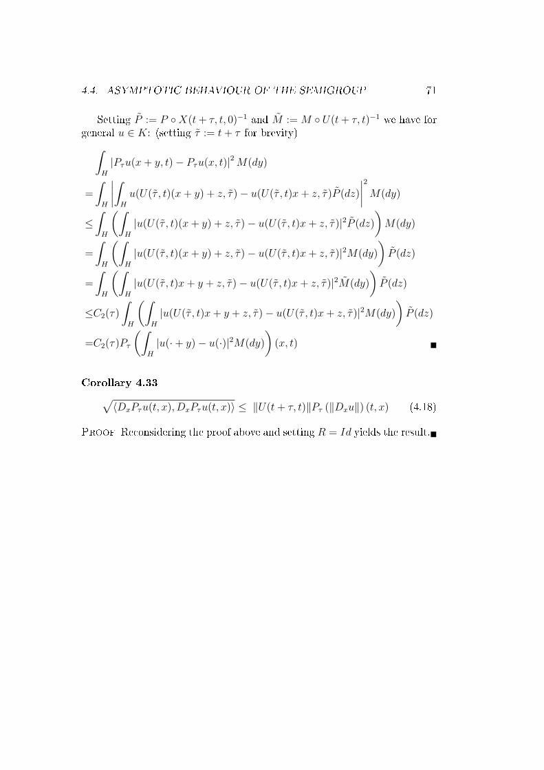
4.4. ASYMPTOTIC BEHAVIOUR OF THE SEMIGROUP 71
Setting P := P X(t + τ, t, 0)−1 and M := M U(t + τ, t)−1 we have forgeneral u ∈ K: (setting τ := t + τ for brevity)∫
H
|Pτu(x + y, t)− Pτu(x, t)|2 M(dy)
=
∫H
∣∣∣∣∫H
u(U(τ , t)(x + y) + z, τ)− u(U(τ , t)x + z, τ)P (dz)
∣∣∣∣2 M(dy)
≤∫
H
(∫H
|u(U(τ , t)(x + y) + z, τ)− u(U(τ , t)x + z, τ)|2P (dz)
)M(dy)
=
∫H
(∫H
|u(U(τ , t)(x + y) + z, τ)− u(U(τ , t)x + z, τ)|2M(dy)
)P (dz)
=
∫H
(∫H
|u(U(τ , t)x + y + z, τ)− u(U(τ , t)x + z, τ)|2M(dy)
)P (dz)
≤C2(τ)
∫H
(∫H
|u(U(τ , t)x + y + z, τ)− u(U(τ , t)x + z, τ)|2M(dy)
)P (dz)
=C2(τ)Pτ
(∫H
|u(·+ y)− u(·)|2M(dy)
)(x, t)
Corollary 4.33√〈DxPτu(t, x), DxPτu(t, x)〉 ≤ ‖U(t + τ, t)‖Pτ (‖Dxu‖) (t, x) (4.18)
Proof Reconsidering the proof above and setting R = Id yields the result.

72 CHAPTER 4. SEMIGROUP AND INVARIANT MEASURE
4.4.2 Functional Inequalities
Following [Röck/Wang03], we will now prove a Poincaré and a Harnack in-equality.
Denition 4.34
ut :=
∫H
u(t, x)νt(dx)
Proposition 4.35 Assume that the νt have uniformly bounded rst mo-ments, that is: supt
∫H‖x‖νt(dx) < ∞ Then we have for all u ∈ K:
limτ→∞
(sup
t|Pτu(t, x)− ut+τ |
)= 0 for every xed x
Proof We have, since ut+τ :=∫
Hu(t+τ, y)νt+τ (dy) = Pt,t+τu(t+τ, ·)(y)νt(dy)
by the property of the evolution system :
|Pτu(t, x)− ut+τ | =∣∣∣∣∫
H
Pt,t+τu(t + τ, ·)(x)− Pt,t+τu(t + τ, ·)(y)νt(dy)
∣∣∣∣≤ ‖DxPt,t+τu(t + τ, ·)‖∞
∫H
|x− y|νt(dy)
≤ ‖U(t + τ, t)‖‖PτDxu(t, ·)‖∞∫
H
|x− y|νt(dy)
≤ Me−ωτ‖Dxu(t + τ, ·)‖∞∫
H
|x− y|νt(dy)τ→∞−→ 0
since the integral is bounded by assumption and ‖Dxu(t, x)‖ = ‖h(t)‖ buth : R → H is continuous and periodic, hence bounded.
Proposition 4.36 (Poincaré Inequality) Given assumption 4.31 and B =Id then we have for C(τ) := max
(∫ τ
0C1(s)ds,
∫ τ
0C2(s)ds
):
Pτu2 − (Pτu)2 ≤ C(τ)PτΓ(u, u) for all τ > 0, u ∈ K (4.19)
Proof Set f(s) := Pτ−s(Psu)2 Then we have by the product rule:
d
dsf(s) = −Pτ−sG(Psu)2 + Pτ−s2PsuGPsu
= −Pτ−s[G(Psu)2 − 2PsuGPsu] = −Pτ−sΓ(Psu, Psu)

4.4. ASYMPTOTIC BEHAVIOUR OF THE SEMIGROUP 73
Hence,
− d
dsf(s) = Pτ−sΓ(Psu, Psu)
= Pτ−s 〈Σ∗∇xPsu, Σ∗∇xPsu〉
+ Pτ−s
∫H
[Psu(x + y, t)− Psu(x, t)]2 M(dy)
≤ C1(s)Pτ−sPs 〈Σ∗∇xu, Σ∗∇xu〉 by (4.15)
+ C2(s)Pτ−sPs
∫H
[u(x + y, t)− u(x, t)]2 M(dy) by (4.16)
Integrating with respect to s and noting that f(0) = Pτf2 and f(t) = (Pτf)2
we obtain:
Pτf2 − (Pτf)2 ≤
(∫ τ
0
C1(s)ds
)Pτ 〈Σ∗∇xu, Σ∗∇xu〉
+
(∫ τ
0
C2(s)ds
)Pτ
∫H
[u(x + y, t)− u(x, t)]2 M(dy)
and the result is proved.
Corollary 4.37 Let be C as in 4.36.Given that C(∞) < ∞ we also have for all u ∈ K:∫
[0,T ]×H
[u(t, x)− ut]2ν(dt, dx) ≤ C(∞)
∫[0,T ]×H
Γ(u, u)ν(dt, dx)
Proof Integrating (4.19) with respect to ν yields, because of invariance:∫[0,T ]×H
u2 − (Pτu)2ν(dt, dx) ≤ C(τ)
∫[0,T ]×H
Γ(u, u)ν(dt, dx)
Letting τ →∞ and using 4.35 together with dominated convergence we have:∫[0,T ]×H
u2 − (ut)2ν(dt, dx) ≤ C(∞)
∫[0,T ]×H
Γ(u, u)ν(dt, dx)

74 CHAPTER 4. SEMIGROUP AND INVARIANT MEASURE
Since u does not depend on x anymore, we have:∫[0,T ]×H
[u(t, x)− ut]2ν(dt, dx) =
∫[0,T ]×H
u2(t, x)− 2u(t, x)ut + u2t ν(dt, dx)
=
∫[0,T ]×H
u2(t, x) + u2t ν(dt, dx)− 2
∫[0,T ]
ut
∫H
u(t, x)νt(dx)︸ ︷︷ ︸ut
dt
=
∫[0,T ]×H
u2(t, x)− u2t ν(dt, dx)
and the result follows.
For the following Harnack inequality we need a denition:
Denition 4.38
ρ(x, y) := inf ‖z‖ :√
Rz = x− y
with the usual convention that inf ∅ = ∞ , so ρ may take the value innityif (x− y) /∈ Im
√R.
The dention of ρ is closely related to the notion of the pseudo inverse, forinformation on that see [Spde07] appendix B. The vague intuition for theterm ρ in the Harnack inequality might be explained as follows: the operator√
R governs the diusion of the underlying equation, if there is no diusionpossible from x to y then we have no result.
Proposition 4.39 (Harnack Inequality)
|Pτu(y)|2 ≤ Pτu2(x) exp
[ρ2(x, y)∫ τ
01
h(s)ds
]for all u ∈ Cb (4.20)
Proof First, let be u ∈ K such that u is strictly positive. SincePτ−s(Psu)2(t, x) will then also be strictly positive we can dene:
Φ(s) := log[Pτ−s(Psu)2(t, xs)]
where xs is given by:
xs := x +(y − x)
∫ s
01
h(τ−u)du∫ τ
01
h(u)du

4.4. ASYMPTOTIC BEHAVIOUR OF THE SEMIGROUP 75
Note that we have x0 = x and xτ = y.Dierentiating Φ we obtain:
d
dsΦ(s) =
dds
Pτ−s(Psu)2(t, xs)
Pτ−s(Psu)2(t, xs)(4.21)
and for the numerator:
d
ds[Pτ−s(Psu)2(t, xs)] =
d
ds[Pτ−s(Psu)2](t, xs) +
⟨Dx[Pτ−s(Psu)2](t, xs),
dxs
ds
⟩= −GPτ−s(Psu)2(t, xs) + Pτ−s[2PsuGPsu](t, xs)
+1
h(τ − s)∫ τ
01
h(u)du
⟨Dx[Pτ−s(Psu)2](t, xs), (y − x)
⟩= −Pτ−sΓ(Psu, Psu)
+1
h(τ − s)∫ τ
01
h(u)du
⟨Dx[Pτ−s(Psu)2](t, xs), (y − x)
⟩(4.22)
We will now estimate 〈Dx[Pτ−s(Psu)2](t, xs), (y − x)〉:
⟨Dx[Pτ−s(Psu)2](t, xs), (y − x)
⟩= inf
z:√
Rz=x−y
⟨Dx[Pτ−s(Psu)2](t, xs),
√Rz⟩
(x− y) ∈ Im√
R
≤√〈RDx[Pτ−s(Psu)2](t, xs), Dx[Pτ−s(Psu)2](t, xs)〉ρ(x, y) Cau.-Schw.
≤ ρ(x, y)√
h(τ − s)Pτ−s
(√〈RDx(Psu)2, Dx(Psu)2〉
)(t, xs) by (4.15)
≤ 2ρ(x, y)√
h(τ − s)Pτ−s
(Psu√〈RDx(Psu), Dx(Psu)〉
)(t, xs) chain rule
(4.23)

76 CHAPTER 4. SEMIGROUP AND INVARIANT MEASURE
Combining (4.21),(4.22) and (4.23) we obtain:
d
dsΦ(s) ≤ −Pτ−sΓ(Psu, Psu)
Pτ−s(Psu)2(t, xs)
+
1h(τ−s)
R τ0
1h(u)
du2ρ(x, y)
√h(τ − s)Pτ−s
(Psu√〈RDx(Psu), Dx(Psu)〉
)(t, xs)
Pτ−s(Psu)2(t, xs)
writing out Γ but omitting the non-local part, we get:
≤ −Pτ−s (〈RDx(Psu), Dx(Psu)〉) (t, xs)
Pτ−s(Psu)2(t, xs)
+
1√h(τ−s)
R τ0
1h(u)
du2ρ(x, y)Pτ−s
(Psu√〈RDx(Psu), Dx(Psu)〉
)(t, xs)
Pτ−s(Psu)2(t, xs)
=1
Pτ−s(Psu)2(t, xs)
× Pτ−s
((Psu)2
[2H
√〈RDx(Psu), Dx(Psu)〉
Psu− 〈RDx(Psu), Dx(Psu)〉
(Psu)2
])(t, xs)
where we have set H := ρ(x,y)√h(τ−s)
R τ0
1h(u)
dufor brevity.
Furthermore, setting G :=
√〈RDx(Psu),Dx(Psu)〉
Psu:
d
dsΦ(s) ≤ 1
Pτ−s(Psu)2(t, xs)Pτ−s
((Psu)2
[−G2 + 2HG
])(t, xs)
=1
Pτ−s(Psu)2(t, xs)Pτ−s
((Psu)2
[−G2 + 2HG−H2 + H2
])(t, xs)
≤ 1
Pτ−s(Psu)2(t, xs)Pτ−s
((Psu)2
[H2])
(t, xs)
= H2

4.4. ASYMPTOTIC BEHAVIOUR OF THE SEMIGROUP 77
since H depends neither on xs nor on t. Integration over s yields:
log[(Pτu)2(t, y)]− log[(Pτu2)(t, x)] = Φ(τ)− Φ(0)
≤∫ τ
0
H2(s)ds
=
∫ τ
0
ρ2(x, y)
h(τ − s)(∫ τ
01
h(u)du)2
ds
=ρ2(x, y)∫ τ
01
h(u)du
Hence, applying the exponential yields:
(Pτu)2(t, y) ≤ Pτu2(t, y)
ρ2(x, y)∫ τ
01
h(u)du
and the proof is complete for positive functions.To obtain the result for general u, note rst, that it is sucient to have itfor |u|, since we have:
|Pτu(t, y)|2 ≤ [Pτ |u|(t, y)]2 ≤ Pτu2(t, x) exp
[ρ2(x, y)∫ τ
01
h(s)ds
]
Of course, we cannot take modulus without leaving K, but as K is an algebrawe may take the square of our functions. Thus, let be u ∈ Cb and ε > 0.Then f :=
√|u| ∈ Cb. Now, by 4.40 we can approximate f pointwisely by
functions un from K. Then, u2n +ε is strictly positive, it will approach |u|+ε
and since the approximating functions are uniformly bounded, we can takelimits in (4.20) and obtain the result via dominated convergence and thenletting ε → 0.
Lemma 4.40 For every f ∈ Cb we can nd a sequence un ∈ K such that:
• un → f pointwisely
• supx,n |un(x)| ≤ 1 + supx |f(x)|

78 CHAPTER 4. SEMIGROUP AND INVARIANT MEASURE
Proof We try to approximate a given f ∈ Cb as follows:Let be (ek)k∈N a complete orthonormal system in D(A∗). Let be
fn(h) := gn(Pnh)
where Pn : H → Rn h 7→ (〈h, e1〉, . . . , 〈h, en〉)and gn : Rn → R (x1, . . . , xn) 7→ f(x1e1 + · · ·+ xnen)
Note that each gn is continuous and bounded and that fn = f onspane1, . . . , en. Moreover, we have Pn → Id strongly and hence fn → fpointwisely.
To obtain an approximation by functions of K we now need to approachevery gn by trigonometric polynomials. So let be g : Rd → R continuous andbounded. For each n ∈ N let be be φn a function that coincides with g on‖x‖∞ ≤ n vanishes on ‖x‖∞ ≥ n+1 and is still continuous. Since φn canbe extended to a continuous (n+1)-periodic function, we can approximate itwith respect to the supremum norm on ‖x‖∞ ≤ n + 1 with trigonometricpolynomials, by Fejér's Theorem. Let us call g(n) an approximation of φn on‖x‖∞ ≤ n + 1 up to 1
n, that is we have:
sup‖h‖∞≤n+1
|g(n)(h)− φn(h)| < 1
n
This implies, of course:
sup‖h‖∞≤n
|g(n)(h)− g(h)| < 1
n
hence, by construction, we have g(n) → g pointwisely for n → ∞ and byperiodicity it is clear that we have supx,n |g(n)(x)| ≤ 1 + supx |g(x)|.
Now, applying the above approximation to our functions gn from above,we denote:
un(h) := f (n)n (h) := g(n)
n (Pnh)
and an easy calculation shows that f(n)n is indeed a function from K, since
we have:
ei〈(k1,...,kn),Pnh〉 = ei〈(k1,...,kn),(〈h,e1〉,...,〈h,en〉)〉
= ei(〈h,k1e1〉+···+〈h,knen〉) = ei〈h,k1e1+···+knen〉

4.4. ASYMPTOTIC BEHAVIOUR OF THE SEMIGROUP 79
and (k1e1 + · · ·+ knen) ∈ D(A∗).
To see that f(n)n (h) → f(h) for each xed h we calculate:
|f(h)− f (n)n (h)| ≤ |f(h)− fn(h)|+ |fn(h)− f (n)
n (h)|
We have already stated that the rst tern will tend to 0. For the second term,note, that for xed h there is N independent of n such that ‖Pnh‖∞ < N .Thus, we obtain:
|fn(h)− f (n)n (h)| = |gn(Pnh)− g(n)
n (Pnh)| ≤ sup‖x‖∞≤N
|gn(x)− g(n)n (x)| < 1
n
whenever n is bigger than N .

80 CHAPTER 4. SEMIGROUP AND INVARIANT MEASURE

Appendix A
Cores
As it is often dicult to describe the action of a generator G on the whole ofits domain D, one would like to nd a subspace, C say, of D which is in somesense tted to G. For example, a space of smooth functions might be suitedto a dierential operator. When this is possible without loss of information,in the sense that the whole generator can be reconstructed from its valueson the test functions, such a C is called a core. Formally:
Denition A.1 Let be G a generator of a strongly continuous semigroup ona Banach space (B, ‖ ‖) with domain D. A subspace C of D is called a corefor G if it is dense in D with respect to the graph norm ‖ ‖G on D, that is‖x‖G := ‖x‖+ ‖Gx‖.
So the above mentioned reconstruction can be carried out by taking theclosure of the graph of the restricted operator. There are other character-izations of a core available. We will cite one and derive another one fromit. The material here is taken from [Arendt86], another useful reference forcores is [Eberle97].
Proposition A.2 Let G be the generator of a strongly continuous semigroupS(t) and let C be a subspace of D(G). If S is the only semigroup, which hasa generator that extends G|C, then C is a core.
We will sketch a proof:Notice that the contraposition of the statement is: If C is not a core thanG|C admits more than one generating extension. So the idea is to construct a
81

82 APPENDIX A. CORES
semigroup T (t) dierent from S, whose generator coincides with G on C. Bya pertubation result, whose proof we omit here, G+P will be a generator forany P that is continuous with respect to the graph norm on D(G). Since wedo not want to change the generator on C, we need a P that vanishes on Cbut not on all of D(G). Since C is not a core, hence not dense in D(G) withrespect to the graph norm, we have the existence of a linear functional f onD(G) continuous for the graph norm, that vanishes on C but not everywhere.(Recall that a subspace is dense if and only if every continuous functionalvanishing there is trivial). Setting P (x) = f(x)u for a xed 0 6= u ∈ D(G)we have the reqired pertubation, and it is clear that G + P 6= G
A complete proof can be found in [Arendt86] page 46.
Lemma A.3 Let S(t) be a strongly continuous semigroup with generator Gon a Banach space B. Let C be a dense subspace of D(G) that is invariantunder S. Then C is a core.
Proof We have to prove, that G is the only generating extension of G|C .Assume A is another generating extension, with semigroup T (t). Considerthe following Cauchy problem, where f ∈ C:
dX(t) = GX(t)dt , X(0) = f
By denition S(t)f is a solution that stays in C by assumption. So S(t)f isalso a solution for the problem:
dX(t) = AX(t)dt , X(0) = f
since G and A coincide on C. Of course T (t)f is also a solution of the secondproblem. As both problems admit a unique solution (see [Pazy74] Chapter4) we conclude S(t)f = T (t)f whenever f ∈ C. As the operators S(t) andT (t) are continuous for any t, and C is dense in B (as it is dense in a densesubset)we have S = T .

Appendix B
Lévy's Continuity Theorem in
Innite Dimensions
In this section we follow [Vakh81]. [Somm07] was helpful.Consider a sequence of probability measures µn on a real separable Hilbertspace H, and the sequence fn of their respective characteristic functions.On Rd Lévy's continuity theorem states, that the pointwise convergence offn to a limit function f , which is continuous in 0, implies that f is the char-acteristic function of some probability measure µ to whom the µn convergeweakly.
On an innite dimensional Hilbert space, this need no longer hold: Letekk∈N be an orthonormal basis of H and let νn be the standard normaldistribution on Rn. Let Tn : Rn → H be an isometric embedding withIm(Tn) = span(e1, ..., en)Then the image measure Tnνn on H will have characteristic function:
fn(h) = e−12
Pnk=1 |〈h,ek〉|2
It is clear, that limn→∞ fn(h) = e−12‖h‖2 =: f(h) and that f is continuous in
the norm topology.Alas, f is not a characteristic function. To see this, note that every charac-teristic function must be even weakly continuous, since
E[ei〈hn,X〉]hn
w→h−→ E[ei〈h,X〉]
holds by dominated convergence.But f is not weakly continuous. We have ek
w→ 0 for k →∞ but f(ek) = e−12
for each k.
83

84 APPENDIX B. LÉVY'S CONTINUITY THEOREM
So, we have to impose stronger conditions on the limit function f toassure that it is itself a characteristic function. It turns out that one has toask for continuity with respect to a weaker topology, the Sazonov topology.
Denition B.1 The Sazonov topology on a Hilbert space H is the coarsesttopology such that the functions
x 7→ 〈Sx, x〉
are continuous for any positive , self-adjoint trace class operator S.
With the help of this denition, we can formulate an extension of Bochner'stheorem:
Theorem B.2 (Sazonov) A functional f on a Hilbert space H is the char-acteristic function of a measure on H, if and only if:
• f is positive denite
• f(0) = 1
• f is continuous in the Sazonov topology
Proof See [Vakh81] 3.1.6
For the proof of 4.10 we have tried to make use of this theorem withoutsuccess. However, we give the underlying idea.Recall that our limit function was essentially of the form:
f(h) := exp
∫ t
−∞λ(Lrh)dr
where the Lr := B∗(r)U∗(t, r) were linear operators.f(0) = 1 is trivial and positive deniteness of the limit is rather easy to show.For the continuity, we know that λ is Sazonov continuous and then it is nothard to show that also λ L is Sazonov continuous for any bounded linearoperator L. Hence, we have pointwise convergence under the integral, and theresult would follow by dominated convergence, if we had an integrable bounduniform in hn as hn → h. Regrettably, we were unable to nd norm-boundedneighborhoods in the Sazonov topology and without those this approachseems to be hopeless.

Bibliography
[Alb/Rue05] Albeverio, R. and Rüdiger, B. : Stochastic Integrals andthe Lévy-Ito Decomposition Theorem on Separable Banach Spaces -Stochastic Analyis and Applications 23, 2005
[App04] Applebaum, David : Lévy Processes and Stochastic Calculus - Cam-bridge University Press, 2004
[App06] Applebaum, David: Martingale-valued measures, Ornstein-Uhlenbeck processes with jumps and operator self-decomposability inHilbert space - Séminaire de Probabilités 39, 2006
[Arendt86] Arendt, Wolfgang in: One-parameter Semigroups of Positive Op-erators - Heidelberg : Springer, 1986
[Chi/Lat99] Chicone, Carmen and Latushkin, Yuri : Evolution Semigroupsin Dynamical Systems and Dierential Equations - Providence : Amer-ican Mathematical Society , 1999
[Chung68] Chung, Kai Lai : A course in probability theory - Academic Press,1968
[Dal/Krei74] Daleckii, Ju. L. and Krein, M. G. : Stability of solutions ofdierential equations in Banach space - Providence : American Mathe-matical Society , 1974
[daPr/Lun07] DaPrato, Guiseppe and Lunardi Alessandra : Ornstein-Uhlenbeck operators with time periodic coeents - Journal of EvolutionEquations 7, 2007
[daPr04] DaPrato, Guiseppe : Kolmogorov Equations for Stochastic PDEs -Birkhäuser, 2004
85

86 BIBLIOGRAPHY
[daPr/zab03] DaPrato, Guiseppe and Zabczyk, Jerzy : Ergodicity for innitedimensional systems - Cambridge University Press, 2003
[Dudley89] Dudley, Richard : Real Analysis and Probability - Wadsworth &Brooks/Cole 1989
[Eberle97] Eberle, Andreas : Uniqueness and Non-Uniqueness of SingularDiusion Operators - University of Bielefeld : Doctorate Thesis, 1997
[Fuhr/Röck00] Fuhrmann, Marco and Röckner, Michael : GeneralizedMehler Semigroups: The Non-Gaussian Case - Potential Analysis 12,2000
[Knab06] Knäble, Kristian : Stochastic Evolution Equations with Lévy Noiseand applications to the Heath-Jarrow-Morton Model - University ofBielefeld : Diploma Thesis, 2006
[Lesc/Röck02] Lescot, Paul and Röckner, Michael : Generators of Mehler-Type Semigroups as Pseudo-Dierential Operators - Innite Dimen-sional Analysis, Quantum Probability and Related Topics 5, 2002
[Lesc/Röck04] Lescot, Paul and Röckner, Michael : Perturbations of Gen-eralized Mehler Semigroups and Applications to Stochastic Heat Equa-tions with Levy Noise and Singular Drift - Potential Analysis 20, 2004
[Linde83] Linde, Werner : Innitely Divisible and Stable Measures on Ba-nach Spaces - Leipzig : Teubner, 1983
[Ma/Röck92] Ma,Zhi-Ming and Röckner,Michael : Introduction to the The-ory of (Non-Symmetric) Dirichlet Forms. - Heidelberg : Springer, 1992
[Nei/Zag07] Neidhardt, Hagen and Zagrebnov, Valentin : Linearnon-autonomous Cauchy problems and evolution semigroups -arXiv:0711.0284v1 [math-ph] 2007
[Pazy74] Pazy, Amnon : Semi-groups of linear operators and applications topartial dierential equations . - College Park Maryland, 1974
[Prott90] Protter, Philip : Stochastic Integration and Dierential Equations- Springer, 1990

BIBLIOGRAPHY 87
[Röck/Wang03] Röckner, Michael and Wang, Feng-Yu : Harnack and func-tional inequalities for generalized Mehler semigroups - Journal of Func-tional Analysis 203, 2003
[Sato99] Sato, Ken-Iti : Lévy processes and innitely divisible distributions- Cambridge University Press , 1999 .
[Spde07] Röckner, Michael and Prevot, Claudia : A Concise Course onStochastic Partial Dierential Equations - Heidelberg : Springer 2007
[Schw73] Schwartz, Laurent : Radon measures on arbitrary topologicalspaces and cylindrical measures . - Oxford : Univ. Pr. , 1973
[Somm07] Sommer, Christian : Lévy's continuity Theorem on Banach Spaces- University of Bielefeld : Bachelor Thesis, 2007
[Stolze05] Stolze, Stefan : Stochastic Equations in Hilbert Space with LévyNoise and their Application in Finance - University of Bielefeld :Diploma Thesis, 2005
[Vakh81] Vakhania, Nikolai : Probability Distributions on Linear Spaces -Elsevier, 1981


![On the Simulation and Estimation of the Mean-Reverting ... · PDF filefunction [ S ] = SimulateOrnsteinUhlenbeckRough( S0, mu, sigma, lambda,deltat, t ) %% Approximate Ornstein-Uhlenbeck](https://img.dokumen.tips/doc/110x75/5aa058dc7f8b9a0d158e08aa/on-the-simulation-and-estimation-of-the-mean-reverting-s-simulateornsteinuhlenbeckrough.jpg)