Embed Size (px)
Citation preview

CONTINUITY PROPERTIES AND INFINITE DIVISIBILITY OF
STATIONARY DISTRIBUTIONS OF SOME GENERALISED
ORNSTEIN-UHLENBECK PROCESSES
ALEXANDER LINDNER AND KEN-ITI SATO
Abstract. Properties of the law � of the integralR1
0c�Nt� dYt are studied, where
c > 1 and f(Nt; Yt); t � 0g is a bivariate L�evy process such that fNtg and fYtgare Poisson processes with parameters a and b, respectively. This is the stationarydistribution of some generalised Ornstein-Uhlenbeck process. The law � is eithercontinuous-singular or absolutely continuous, and su�cient conditions for each caseare given. Under the condition of independence of fNtg and fYtg, it is shown that �is continuous-singular if b=a is su�ciently small for �xed c, or if c is su�ciently largefor �xed a and b, or if c is in the set of Pisot-Vijayaraghavan numbers, which includesall integers bigger than 1, for any a and b, and that, for Lebesgue almost every c, �is absolutely continuous if b=a is su�ciently large. The law � is in�nitely divisibleif fNtg and fYtg are independent, but not in general. Complete characterisationof in�nite divisibility is given for � and for the symmetrisation of �. Under thecondition that � is in�nitely divisible, the continuity properties of the convolutionpower �t� of � are also studied. Some results are extended to the case where fYtgis an integer valued L�evy process with �nite second moment.
1. Introduction
A generalised Ornstein-Uhlenbeck process fVt; t � 0g with initial condition V0 isde�ned as
Vt = e��t�V0 +
Z t
0
e�s� d�s
�;
where f(�t; �t); t � 0g is a bivariate L�evy process, independent of V0. See Carmona etal. [3], [4] for basic properties. Such processes arise in a variety of situations such asrisk theory (e.g. Paulsen [17]), option pricing (e.g. Yor [25]) or �nancial time series(e.g. Kl�uppelberg et al. [12]), to name just a few. They also constitute a naturalcontinuous time analogue of random recurrence equations, as studied by de Haan andKarandikar [11]. Lindner and Maller [15] have shown that a generalised Ornstein-Uhlenbeck process admits a strictly stationary solution which is not degenerate to aconstant process with a suitable V0 if and only if
(1.1)
Z 1�
0
e��s� dLs := limt!1
Z t
0
e��s� dLs
exists and is �nite almost surely and not degenerate to a constant random variable.Here, f(�t; Lt); t � 0g is another bivariate L�evy process, de�ned in terms of f(�t; �t)g
1

by
Lt = �t +X0<s�t
(e�(�s��s�) � 1)(�s � �s�)� ta1;2�;�;
where a1;2�;� denotes the (1; 2)-element in the Gaussian covariance matrix of the L�evy-Khintchine triplet of f(�t; �t)g. Conversely, f(�t; �t)g can be reconstructed fromf(�t; Lt)g by
�t = Lt +X0<s�t
(e�s��s� � 1)(Ls � Ls�) + ta1;2�;L:
The distribution of (1.1) then gives the unique stationary distribution. When theintegral (1.1) converges was characterised by Erickson and Maller [6] and generalisedby Kondo et al. [13] to the case when f(�t; Lt)g is an R�Rd valued L�evy process withd 2 N.
Suppose now that f(�t; Lt)g is a bivariate L�evy process such that (1.1) convergesalmost surely and is �nite, and denote by
� := L�Z 1�
0
e��s� dLs
�the distribution of the integral. If �t = t is deterministic, then it is well known that� is self-decomposable, hence is in�nitely divisible as well as absolutely continuous(if not degenerate to a constant, which happens only if fLtg is also deterministic).Other cases where � is self-decomposable include the case where f�tg is stochastic,but spectrally negative (cf. Bertoin et al. [1]). On the other hand, as remarked bySamorodnitsky, � is not in�nitely divisible if e.g. �t = Nt+�t with a Poisson processfNt; t � 0g and a positive drift � > 0 and Lt = t (cf. Kl�uppelberg et al. [12], p. 408).Continuity properties of � for general f(�t; Lt)g were studied by Bertoin et al. [1], whoshowed that � cannot have atoms unless � is a Dirac measure, with this degeneratecase also being characterised. Gjessing and Paulsen [8] derived the distribution of �in a variety of situations; however, in all cases considered the distribution turned outto be absolutely continuous.
With these results in mind, it is natural to ask whether � will always be absolutelycontinuous for general f(�t; Lt)g, unless � degenerates to a Dirac measure. That thisis not the case, even when f�tg and fLtg are assumed to be independent, will beshown in the present article. More precisely, we will study in detail
(1.2) � = L�Z 1�
0
e�(log c)Ns� dYs
�= L
�Z 1�
0
c�Ns� dYs
�;
where c is a constant greater than 1 and fNtg and fYtg are both Poisson processeswith parameters a and b, respectively, and with f(Nt; Yt)g being a bivariate L�evyprocess. The integral in (1.2) is then an improper Stieltjes integral pathwise. Fromthe strong law of large numbers, we see that the integral exists and is �nite. Let Tbe the �rst jump time of fNtg. ThenZ 1�
0
c�Ns� dYs = YT +
Z 1�
T
c�Ns� dYs = YT + c�1Z 1�
0
c�N0
s� dY 0s ;
2

where f(N 0t ; Y
0t )g is an independent copy of f(Nt; Yt)g. Hence, letting � = L(YT ), we
obtain
(1.3) b�(z) = b�(z) b�(c�1z); z 2 R;where b�(z) and b�(z) denote the characteristic functions of � and �. It follows that
b�(z) = b�(c�kz) k�1Yn=0
b�(c�nz); k 2 N;
and hence
(1.4) b�(z) = 1Yn=0
b�(c�nz):In general, if a distribution � satis�es (1.3) with some distribution �, then � is calledc�1-decomposable. Our study of the law � is based on this c�1-decomposability. Theexpression (1.4) shows that the law � controls �. The properties of c�1-decomposabledistributions are studied by Wolfe [24], Bunge [2], Watanabe [22] and others. In par-ticular, it is known that any non-degenerate c�1-decomposable distribution is eithercontinuous-singular or absolutely continuous (Wolfe [24]). A distribution � is self-
decomposable if and only if � is c�1-decomposable for all c > 1. In this case � and �are in�nitely divisible. In general if a distribution � satis�es (1.3) with � being in�n-itely divisible, then � is called c�1-semi-selfdecomposable. For the law � in (1.2), weare interested in the Hausdor� dimension dim (�) of �, de�ned as the in�mum of theHausdor� dimensions of E over all Borel sets E satisfying �(E) = 1 (in some papersincluding [22], this is called upper Hausdor� dimension and denoted by dim�(�)).Watanabe [22] shows that, if a distribution � is c�1-decomposable satisfying (1.3)with a discrete distribution �, then dim (�) � H(�)= log c, where H(�) is the entropyof �. It follows that the law � in (1.2) is continuous-singular if H(�)= log c < 1.
In Section 2 we will concentrate on the case where fNtg and fYtg are independent.The law � is determined by c and q = b=(a + b), and so it is denoted by �c;q. Wewill show that �c;q is continuous-singular if q is su�ciently small for �xed c, or if c issu�ciently large for �xed q, or if c is a Pisot-Vijayaraghavan (P.V.) number for anyq. Further we will show that if c�1 is a Peres-Solomyak (P.S.) number, then �c;q isabsolutely continuous for q su�ciently close to 1.
In Section 3 we treat the case where the independence of fNtg and fYtg is notassumed. The L�evy process f(Nt; Yt)g then has L�evy measure concentrated on thethree points (1; 0), (0; 1) and (1; 1) and the amounts of the measure of these pointsare denoted by u, v and w. Letting p = u=(u + v + w), q = v=(u + v + w) andr = w=(u+ v + w), we will see that � is determined by c, q and r, and � is by q andr, and hence denote � = �c;q;r and � = �q;r. We call r the dependence parameter off(Nt; Yt)g, since r = 0 is equivalent to independence of fNtg and fYtg and r = 1 meansfNtg = fYtg. If r = 0, then � = L(YT ) is in�nitely divisible as is seen from subordina-tion theory, and hence � is also in�nitely divisible. But, if r > 0, the situation is morecomplicated. We will give complete description of the condition of in�nite divisibilityof �c;q;r and �q;r in terms of their parameters. It will turn out that in�nite divisibility
3

of �c;q;r does not depend on c. It is shown in Niedbalska-Rajba [16] that there existsa c�1-decomposable in�nitely divisible distribution � that satis�es (1.3) with a non-in�nitely-divisible �. But, in our case, it will turn out that �c;q;r is in�nitely divisibleif and only if �q;r is so. We also address the problem of in�nite divisibility of the sym-metrisations �sym and �sym of � and �. In�nite divisibility of a distribution impliesthat of its symmetrisation, but there is a non-in�nitely-divisible distribution whosesymmetrisation is in�nitely divisible, which is pointed out in pp. 81{82 in Gnedenkoand Kolmogorov [9]. Complete description of in�nite divisibility of �sym and �sym
will be given, which provides new examples of this phenomenon in [9]. In the proofof non-in�nite-divisibility in Section 3, we use three methods: (1) Katti's conditionfor distributions on nonnegative integers; (2) L�evy-Khintchine type representation ofcharacteristic functions with signed measures in place of L�evy measures; (3) repre-sentation of the Laplace transforms of in�nitely divisible distributions on [0;1) inthe form e�'(�) with '0(�) being completely monotone.
In the latter half of Section 2 we consider a more general bivariate L�evy processf(Nt; Yt)g with independent components, where fNtg is a Poisson process and fYtgis an integer valued L�evy process with �nite second moment. The law � in (1.2) withc > 1 is still c�1-semi-selfdecomposable and in�nitely divisible. We will study theconvolution power �t� of �, that is, the distribution at time t of the L�evy processassociated with �. We will show that �t� is continuous-singular if t is su�cientlysmall for �xed c, or if c is su�ciently large for �xed t, or if c is a P.V. number for anyt, and that �t� is absolutely continuous if c�1 is a P.S. number and t is su�cientlylarge. Thus the present paper provides a new class of examples of L�evy processeswith distribution changing from continuous-singular to absolutely continuous as timepasses. See Section 27 in Sato [20] and Watanabe's survey [23] for such time evolutionof L�evy processes. We emphasise that here the distribution � arises naturally as thestationary distribution of a generalised Ornstein-Uhlenbeck process.
We remark that Theorem 3.2 of Kondo et al. [13] on the law � of the form (1.2)with c = e, fNtg Poisson and fNtg and fYtg independent can be extended to generalc > 1 without any change of the proof, and that Remark 3.3 of the same paper pointsout that such a distribution is either continuous-singular or absolutely continuous.This was the starting point of our research.
Throughout the paper, the set of all positive integers will be denoted by N =f1; 2; 3; : : :g, while we set N0 = N[f0g. The set of integers is denoted by Z. The Diracmeasure at a point x will be denoted by �x. For general de�nitions and propertiesregarding L�evy processes and in�nitely divisible distributions, we refer to Sato [20].
2. Continuity properties in the independent case
The �st task in this section is to establish the c�1-decomposability of the lawin (1.2). Since this property prevails in a wider range, we formulate a more generalresult.
Proposition 2.1. Suppose that f(�t; Lt)g is a bivariate L�evy process having the fol-
lowing properties: �t = (log c)e�t with c > 1 and with fe�tg being a compound Poisson
4

process with L�evy measure supported on f: : : ;�2;�1g [ f1g and Ee�t > 0 for t > 0,and fLtg is a L�evy process with �nite log-moment. Let � be de�ned as
(2.1) � := L�Z 1�
0
e��s�dLs
�= L
�Z 1�
0
c�e�s�dLs
�:
Then � is c�1-decomposable satisfying (1.3) with
(2.2) � = L�Z T
0
c�e�s�dYs
�;
where T is the hitting time of 1 for fe�tg.Proof. Let fFt; t � 0g be the natural completed �ltration of f(�t; Lt); t � 0g. ThenT is a stopping time with respect to fFt; t � 0g. The process fe�tg moves by jumps of
the height 2 f: : : ;�2;�1g[f1g and satis�es e�t !1 as t!1. Hence T is �nite a. s.Existence and �niteness of the integral in (2.1) follows from Theorem 2 of Ericksonand Maller [6]. From the L�evy process version of the strong Markov property, weobtain
Z :=
Z 1�
0
c�e�s� dLs =
Z T
0
c�e�s� dLs + c�1
Z 1�
T+
c�(e�s��e�T ) d(L� � LT )s
= W + c�1Z 0; say,
where Z and Z 0 both have law �, W is FT -measurable and Z 0 is independent of FT .This implies (1.3) with � = L(W ), that is, with � of (2.2). �
As in Watanabe [22], we use two classes of numbers, namely Pisot-Vijayaraghavan(P.V.) numbers (sometimes called Pisot numbers) and Peres-Solomyak (P.S.) num-bers. A number c > 1 is called a P.V. number if there exists a polynomial F (x) withinteger coe�cients with leading coe�cient 1 such that c is a simple root of F (x) andall other roots have modulus less than 1. Every positive integer greater than 1 is aP.V. number, but also (1 +
p5)=2 or the unique real root of x3 � x� 1 = 0 are non-
trivial examples. There exist countably in�nitely many P.V. numbers which are notintegers. See Peres, Schlag and Solomyak [18] for related information. On the otherhand, following Watanabe [22], we call c�1 a P.S. number if c > 1 and if there arep 2 (1=2; 1) and k 2 N such that the kth power of the characteristic function of thedistribution of
P1n=0 c
�nUn, where fUng is i. i. d. with P [Un = 0] = 1�P [Un = 1] = p,is integrable. Watanabe [22] pointed out that the paper [19] of Peres and Solomyakcontains the proof that the set of P.S. numbers in the interval (0; 1) has Lebesguemeasure 1. However, according to [22], an explicit example of a P.S. number is notknown so far. As follows from the results of [22], the set of P.V. numbers and the setof reciprocals of P.S. numbers are disjoint. The entropy H(�) of a discrete probabilitymeasure � on R is given by
H(�) := �Xa2C
�(fag) log �(fag);
5

where C is the carrier of �. Here, as in [20], a measure � on R is said to be discrete ifthere is a countable set C such that �(R n C) = 0. The carrier of a discrete measureis the set of points with positive mass.
Now we can formulate one of our main results.
Theorem 2.2. Assume that fNt; t � 0g and fYt; t � 0g are independent Poisson
processes with parameters a > 0 and b > 0, respectively. Let
(2.3) q := b=(a+ b)
and
(2.4) �c;q := L�Z 1�
0
c�Ns� dYs
�with c > 1. Let
(2.5) h(q) :=1
1� qlog
1
1� q� q
1� qlog
q
1� q:
Then the following are true:
(a) The Hausdor� dimension of �c;q is estimated as
(2.6) dim (�c;q) � h(q)
log cfor all c > 1 and q 2 (0; 1):
(b) If c is a P.V. number, then �c;q is continuous-singular for all q 2 (0; 1).(c) If c�1 is a P.S. number, then there are constants 0 < q0 � q1 < 1 such that
�c;q is continuous-singular for all q 2 (0; q0), absolutely continuous without bounded
continuous density for all q 2 (q0; q1) if q0 < q1, and absolutely continuous with
bounded continuous density for all q 2 (q1; 1).
The estimate (2.6) is meaningful only when h(q)= log c < 1, as the Hausdor�dimension of any measure on the line is less than or equal to 1. In Theorem 2.2 thelaw � in (1.2) depends only on c and q, as will be seen in the proof. The functionh(q) is continuous and strictly increasing on (0; 1) and tends to 0 as q # 0 in the speedh(q) � q log(1=q). Under the same assumption we have the following consequences.
Corollary 2.3. (a) Fix c > 1. If q 2 (0; 1) is such that h(q) < log c, then �c;q is
continuous-singular.
(b) Let c > 2. If
0 < q < 1� (log 2= log c);
then �c;q is continuous-singular.(c) Fix q > 0. If c > eh(q), then �c;q is continuous-singular.
For example of (b), in the case c = e, �e;q is continuous-singular if
q < 1� log 2 � 0:30685:
In the case q = 1=2, (c) says that �c;1=2 is continuous-singular if c > 4.
6

Proof of Corollary 2.3. Assertions (a) and (c) are clear from (2.6), since probabilitymeasures with Hausdor� dimension < 1 are singular and since �c;q is continuous, aswill be seen in the proof of Theorem 2.2. Assertion (b) is a consequence of (a), since
h(q) =1
1� q
�(1� q) log
1
1� q+ q log
1
q
�� 1
1� qlog 2
by concavity of the function log x. �
Proof of Theorem 2.2. Notice that, by Proposition 2.1, �c;q is c�1-decomposable and
T is now the �rst jump time of fNtg. The law of T is exponential with parameter aand the law � in (2.2) equals L(YT ). This law � = L(YT ) is geometric with parameterp, i.e.,
�(fkg) = pqk; k 2 N0;
where p = 1� q = a=(a+ b). Indeed, using the independence of fNtg and fYtg,
�(fkg) = P (YT = k) =
Z 1
0
P (Yt = k)ae�atdt
=
Z 1
0
e�btbktk
k!ae�atdt =
a
a+ b
�b
a+ b
�k
:
Hence � is compound Poisson with L�evy measure
am := ��(fmg) = qm=m; m 2 N;that is,
(2.7) b�(z) = exp
"1X
m=1
(eimz � 1)am
#:
Thus it follows from (1.4) that � = �c;q is in�nitely divisible with characteristicfunction
(2.8) b�(z) = exp
"1Xn=0
1Xm=1
(eimc�nz � 1)am
#:
The entropy H(�) of � equals h(q), since
(2.9) H(�) = �p(log p)1Xk=0
qk � p(log q)1Xk=0
kqk = � log p� q
plog q:
Now we obtain assertion (a) from Theorem 2.2 of Watanabe [22].Let us prove (b). Assume that c is a P.V. number. The following proof of
continuous-singularity of � = �c;q is based on an idea of Erd}os [5] as in [22]. Since �is c�1-decomposable and non-degenerate, Wolfe's theorem in [24] (or Theorem 27.15of [20]) tells us that � is either continuous-singular or absolutely continuous. Soit is enough to show that it is not absolutely continuous. Thus, by virtue of theRiemann{Lebesgue theorem, it is enough to �nd a sequence zk !1 such that
lim supk!1
jb�(zk)j > 0:
7
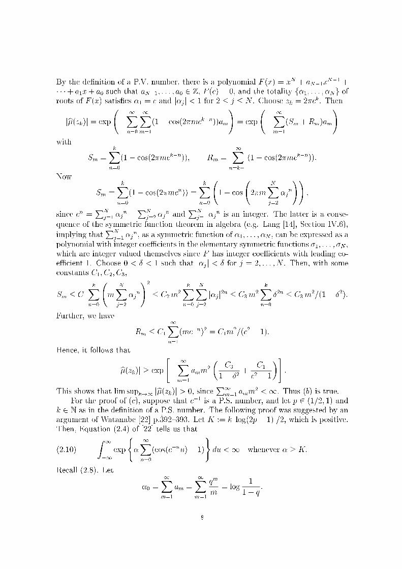
By the de�nition of a P.V. number, there is a polynomial F (x) = xN + aN�1xN�1 +
� � �+ a1x+ a0 such that aN�1; : : : ; a0 2 Z, F (c) = 0, and the totality f�1; : : : ; �Ng ofroots of F (x) satis�es �1 = c and j�jj < 1 for 2 � j � N . Choose zk = 2�ck. Then
jb�(zk)j = exp
�
1Xn=0
1Xm=1
(1� cos(2�mck�n))am
!= exp
�
1Xm=1
(Sm +Rm)am
!with
Sm =kX
n=0
(1� cos(2�mck�n)); Rm =1X
n=k+1
(1� cos(2�mck�n)):
Now
Sm =kX
n=0
(1� cos(2�mcn)) =kX
n=0
1� cos
2�m
NXj=2
�jn
!!;
since cn =PN
j=1 �jn �PN
j=2 �jn and
PNj=1 �j
n is an integer. The latter is a conse-quence of the symmetric function theorem in algebra (e.g. Lang [14], Section IV.6),
implying thatPN
j=1 �jn, as a symmetric function of �1; : : : ; �N , can be expressed as a
polynomial with integer coe�cients in the elementary symmetric functions �1; : : : ; �N ,which are integer valued themselves since F has integer coe�cients with leading co-e�cient 1. Choose 0 < � < 1 such that j�jj < � for j = 2; : : : ; N . Then, with someconstants C1; C2; C3,
Sm � C1
kXn=0
m
NXj=2
�jn
!2
� C2m2
kXn=0
NXj=2
j�jj2n � C3m2
kXn=0
�2n � C3m2=(1� �2):
Further, we have
Rm � C1
1Xn=1
(mc�n)2 = C1m2=(c2 � 1):
Hence, it follows that
jb�(zk)j � exp
"�
1Xm=1
amm2
�C3
1� �2+
C1
c2 � 1
�#:
This shows that lim supk!1 jb�(zk)j > 0, sinceP1
m=1 amm2 <1. Thus (b) is true.
For the proof of (c), suppose that c�1 is a P.S. number, and let p 2 (1=2; 1) andk 2 N as in the de�nition of a P.S. number. The following proof was suggested by anargument of Watanabe [22] p. _392{393. Let K := kj log(2p� 1)j=2, which is positive.Then, Equation (2.4) of [22] tells us that
(2.10)
Z 1
�1
exp
(�
1Xn=0
(cos(c�nu)� 1)
)du <1 whenever � � K:
Recall (2.8). Let
�0 =1X
m=1
am =1X
m=1
qm
m= log
1
1� q:
8

Then it follows from Jensen's inequality thatZ 1
�1
jb�(z)jdz = 2
Z 1
0
exp
"1
�0
1Xm=1
am
�0
1Xn=0
(cos(mc�nz)� 1)
!#dz
� 2
Z 1
0
"1
�0
1Xm=1
am exp
�0
1Xn=0
(cos(mc�nz)� 1)
!#dz
=2
�0
1X
m=1
amm
!Z 1
0
exp
�0
1Xn=0
(cos(c�nu)� 1)
!du:
The latter is �nite whenever �0 � K by (2.10), that is, whenever q � 1� e�K . Hence� is absolutely continuous with bounded continuous density if q � 1 � e�K . On theother hand we know from (a) that � is continuous-singular for small enough q. Theexpression (2.8) shows that � has L�evy measure
(2.11) �� =1Xn=0
1Xm=1
qm
m�c�nm;
which is increasing in q 2 (0; 1). Thus �c;q0 is a convolution factor of �c;q if q0 < q.
Thus, recalling Lemma 27.1 of [20], we obtain assertion (c). �
Keeping the assumptions that fNtg is a Poisson process and that fNtg and fYtgare independent, we will allow fYtg more general than in Theorem 2.2. We cannotgive the properties of � itself (except when c is a P.V. number), but we describe theproperties of the convolution power �t� of �.
Theorem 2.4. Assume that fNtg is a Poisson process and fYtg is an integer valued
L�evy process, not identically zero, with �nite second moment, and that fNtg and fYtgare independent. Let
(2.12) �c := L�Z 1�
0
c�Ns� dYs
�;
where c > 1. Let T be the �rst jump time of fNtg and let � = L(YT ). Then the
following are true.
(a) The entropy H(�t�) is a �nite, continuous, strictly increasing function of t 2[0;1), vanishing at t = 0.(b) It holds true that
(2.13) dim (�ct�) � H(�t�)
log cfor all t � 0 and c > 1:
(c) If c is a P.V. number, then �ct� is continuous-singular for all t > 0.
(d) If c�1 is a P.S. number, then there are t0 and t1 with 0 < t0 � t1 <1 such that
�ct� is continuous-singular for all t 2 (0; t0), absolutely continuous without bounded
continuous density for all t 2 (t0; t1) if t0 < t1, and absolutely continuous with boundedcontinuous density for all t 2 (t1;1).
9
Corollary 2.5. For each c > 1, �ct� is continuous-singular for all su�ciently small
t > 0. For each t > 0, �ct� is continuous-singular for all su�ciently large c > 1.
This is an obvious consequence of (a) and (b) of the theorem.
Lemma 2.6. If � is a distribution on Z with �nite absolute moment of order 1 + "for some " > 0, then its entropy H(�) is �nite.
Proof. Let � =P1
m=�1 pm�m. ThenP1
m=�1 jmj1+"pm < 1. Hence there is a con-stant C > 0 such that pm � Cjmj�1�". The function f(x) = x log(1=x) is increasingfor 0 � x � e�1. Hence,
H(�) �X
jmj�m0
pm log(1=pm) +X
jmj>m0
Cjmj�1�" log((Cjmj�1�")�1) <1
with an appropriate choice of m0. �
Proof of Theorem 2.4. By Proposition 2.1, � is c�1-decomposable satisfying (1.3) with� = L(YT ). Since fYtg is integer valued, � is a distribution on Z. Since, for some con-stant C > 0, E[Y 2
t ] � C(t+ t2) for all t � 0 and since T is exponentially distributed,
E[YT2] =
Z(0;1)
E[Ys2]P [T 2 ds] � C
Z(0;1)
(s+ s2)P [T 2 ds] <1:
Lemma 2.6 then shows that H(�) < 1. Notice that � is the distribution at time1 of the L�evy process fYTtg obtained by subordination of fYtg by an independentgamma subordinator fTtg. The process fYTtg has drift 0, since it is integer valued(use Corollary 24.6 of [20]; another proof is to use Theorem 30.10 of [20]). Thus �is compound Poisson. In particular, �c is c
�1-semi-selfdecomposable. We obtain (a)from Proposition 5.1 of Watanabe [22] or Exercise 29.24 of Sato [20]. The propertyof being c�1-semi-selfdecomposable is inherited by going to convolution powers, since(1.3) implies d�ct�(z) = c�t�(z)d�ct�(c�1z)for any t � 0. Then, applying Theorem 2.2 of [22] to the law �c
t�, we get (b). Thecharacteristic function of � is given by
b�(z) = exp
0@ Xm2Znf0g
(eimz � 1)am
1A ; z 2 R;
with some am � 0 satisfyingP
m2Znf0gm2am <1. The latter is because � has �nite
second moment. Hence the proof of (c) is given entirely in the same way as thatof Theorem 2.2 (b). If c�1 is a P.S. number and t is su�ciently large, then �c
t� isabsolutely continuous with bounded continuous density, which is shown in the sameway as Theorem 2.2 (c), or we can apply Theorem 2.1 of Watanabe [22]. This proves(d). �
In the set-up of Theorem 2.2, the distribution � is geometric with parameter1� q. Thus, the estimate of H(�t�) for this � is of some interest, in connection withthe estimate (2.13) of Theorem 2.4.
10

Proposition 2.7. If � is geometric with parameter 1� q, then
(2.14) H(�t�) � t
�1
p(1 + 2 log
1
p) +
q
plog
1
t
�for 0 < t � 1;
where p = 1� q.
Proof. The distribution �t�, t > 0, is negative binomial distribution with parameterst and p, i.e.,
�t�(fkg) =��tk
�pt(�q)k; k 2 N0:
To estimate H(�t�) from above, observe that, for 0 < t � 1 and k 2 N,t ptqk=k � �t�(fkg) � t qk;
so that
H(�t�) = �1Xk=0
�t�(fkg) log �t�(fkg)
� �(log pt) +1Xk=1
tqk�log k � log(tpt)� k log q
�� t
�log
1
p+
1
plog
1
p� q
plog(tpt)� q
p2log q
�;
where we usedP1
k=1 k qk = q=p2 and
1Xk=1
qk log k �1Xk=1
qkkX
n=1
1
n=
1
plog
1
p;
cf. Gradshteyn and Ryzhik [10], Formula 1.513.6. Recalling that pt � p since t � 1,this can be further estimated to
H(�t�) � t
�2
plog
1
p+q
plog
1
t+
q
p2log
1
q
�:
Together with (q=p) log(1=q) = (q=p) log(1 + p=q) � 1, this gives (2.14). �
Let gq(t) denote the function on the right-hand side of (2.14). This is continuousand strictly increasing on (0; 1] with limt#0 gq(t) = 0. For �c;q of (2.4), we can estimatedim (�c;q
t�) by gq(t)= log c if 0 < t � 1.
The following proposition explains why Theorems 2.2 and 2.4 have similarity. Wesay that fUq; 0 � q < 1g is an additive process if it is stochastically continuous, withindependent increments, starting at the origin and having cadlag paths.
Proposition 2.8. Fix c > 1. Then there exists an additive process fUq; 0 � q < 1gwith time parameter q 2 [0; 1) such that L(Uq) equals �c;q of (2.4) for q > 0 and
L(U0) = �0.
11
Proof. As we observed in the proof of Theorem 2.2, �c;q has characteristic function(2.8) and its L�evy measure (2.11) is increasing in q 2 (0; 1). Furthermore, for eachz, b�c;q(z) is continuous in q 2 (0; 1) and tends to 1 as q # 0. Hence we can applythe analogue of Theorem 9.7 of [20] to time parameter running on [0; 1) and �nd anadditive process in law corresponding to �c;q. It has a cadlag modi�cation by theanalogue of Theorem 11.5 of [20]. �
3. The dependent case: infinite divisibility and continuity properties
In Theorem 2.2 we studied the law �c;q ofR1�
0c�Ns� dYs in the case where fNtg
and fYtg were independent Poisson processes. In particular, we showed in�nite di-visibility of �c;q. In this section we relax the assumption of independence. Supposethat f(Nt; Yt); t � 0g is a bivariate L�evy process such that fNtg is a Poisson pro-cess with parameter a > 0 and fYtg is a Poisson process with parameter b > 0. Itthen follows easily that f(Nt; Yt)g has no Gaussian part, zero drift, and L�evy mea-sure �(N;Y ) concentrated on the set f(1; 0); (0; 1); (1; 1)g, consisting of three points(e.g. [20], Proposition 11.10). Denote
u := �(N;Y )(f(1; 0)g); v := �(N;Y )(f(0; 1)g); and w := �(N;Y )(f(1; 1)g):Then u; v; w � 0, u+ w = a and v + w = b. Let
p :=u
u+ v + w; q :=
v
u+ v + w; r :=
w
u+ v + w;
so that p; q; r 2 [0; 1], p + q + r = 1, p + r > 0 and q + r > 0. If r = 0, then fNtgand fYtg are independent, the case which was treated in Theorem 2.2. If r = 1, thenfNtg = fYtg. So we call r the dependence parameter of f(Nt; Yt)g. For c > 1 denote
(3.1) �c;q;r := L�Z 1�
0
c�Ns� dYs
�;
where the almost sure convergence to a �nite random variable follows again fromErickson and Maller [6] or directly from the strong law of large numbers. If r = 0,then �c;q;r equals �c;q of (2.4) in Theorem 2.2. If r = 1 (i.e. p = q = 0), then it followsfrom fNtg = fYtg thatZ 1�
0
c�Ns� dYs =
Z 1�
0
c�Ns�dNs =1Xj=0
c�j =c
c� 1;
which is degenerate to a constant. So throughout this section we will assume thatp + q > 0 in addition to the above mentioned conditions p + r > 0 and q + r > 0.That is, p; q; r < 1. All propositions and theorems in this section are in this set-up. By Theorem 2.2 in Bertoin et al. [1], �c;q;r will then not degenerate to a Diracmeasure, hence will be a continuous distribution. More strongly, since Proposition2.1 is applicable, �c;q;r is c
�1-decomposable and, by virtue of Wolfe's theorem in [24],�c;q;r is either continuous-singular or absolutely continuous. We de�ne �q;r in thefollowing way: if q > 0, denote by �q a geometric distribution with parameter 1� q,i.e. �q(fkg) = (1� q)qk for k = 0; 1; : : :, and denote
(3.2) � = �q;r := (1 + r=q)�q � (r=q)�0;
12
so that �q;r is a probability distribution concentrated on N0 with
(3.3) �q;r(f0g) = (1 + r=q)(1� q)� (r=q) = 1� q � r = p ;
if q = 0, let �0;r be a Bernoulli distribution with parameter r 2 (0; 1), i.e.
(3.4) �0;r(f1g) = 1� �0;r(f0g) = r:
Proposition 3.1. We have
(3.5) b�c;q;r(z) = b�q;r(z) b�c;q;r(c�1z); z 2 R:In particular, �c;q;r is c
�1-decomposable and determined by c, q and r.
Proof. Since we can use Proposition 2.1, we have only to show that L(YT ) = �q;r,where T is the time of the �rst jump of fNtg, i.e. the time of the �rst jump off(Nt; Yt)g with size in f(1; 0); (1; 1)g. Let Si 2 R
2 be the size of the ith jump off(Nt; Yt)g. Then we have for k � 1
YT = k () [S1 = : : : = Sk�1 = (0; 1); Sk = (1; 1)]
or [S1 = : : : = Sk = (0; 1); Sk+1 = (1; 0)]
as well asYT = 0 () S1 = (1; 0):
SinceP [Si = (1; 0)] = p; P [Si = (0; 1)] = q; P [Si = (1; 1)] = r;
it follows that P (YT = 0) = p and, for k � 1, P (YT = k) = qk�1r + qkp. From thisfollows easily that L(YT ) = �q;r for q > 0, while it is a Bernoulli distribution withparameter r for q = 0. �
It is of interest whether �c;q;r is in�nitely divisible or not. It is also of interestwhether the symmetrisation (�c;q;r)
sym of �c;q;r is in�nitely divisible or not. Recallthat the symmetrisation �sym of a distribution � is de�ned to be the distribution withcharacteristic function d�sym(z) = jb�(z)j2, z 2 R. If X is a random variable such thatL(X) = � and X 0 is an independent copy of X, then �sym = L(X�X 0). Thus in�nitedivisibility of � implies that of �sym, but the converse is not true, as is mentionedin the Introduction. Before going to �c;q;r, we will �rst settle the question of in�nitedivisibility of �q;r and (�q;r)
sym.
Lemma 3.2. Assume q > 0 and let � = �q;r. Then the following hold true:
(a) If r � pq, or if p = 0, then � is in�nitely divisible.
(b) If r > pq and p > 0, then � is not in�nitely divisible.
(c) If r > pq and p > 0, then �sym is in�nitely divisible if and only if
(3.6) p � qr:
We remark that if 0 � � � 1, then (1 � �)�q + ��0 is in�nitely divisible, sinceconvex combinations of two geometric distributions are in�nitely divisible (see pp.379{380 in Steutel and van Harn [21]), and the Dirac measure �0 is a limit of geometricdistributions. Assertions (a) and (b) of the lemma above show in what extent thisfact can be generalised to negative �.
13

Proof of Lemma 3.2. The characteristic function of � is given by
(3.7) b�(z) = (1 + r=q)b�q(z)� r=q = (1 + r=q)1� q
1� qeiz� r=q =
p+ reiz
1� qeiz; z 2 R:
(a) If p = 0, then �(f0g) = 0 by (3.3), and �(fkg) = (1 + (1 � q)=q)(1 � q)qk =(1 � q)qk�1 for k = 1; 2; : : :, and thus � is a geometric distribution translated by 1,hence in�nitely divisible. So assume that r � pq. Then p > 0 (otherwise p = r = 0,contradicting p+ r > 0). Since p = (1� q)=(1 + r=p), it follows from (3.7) that
b�(z) = exp
�log(1� q)� log
�1 +
r
p
�+ log
�1 +
r
peiz�� log(1� qeiz)
�:
Hence
(3.8) b�(z) = exp
"1Xk=1
(eikz � 1)qk
k
1�
�� r
pq
�k!#
:
Recall that r=(pq) � 1. It follows that � is in�nitely divisible with L�evy measure��(fkg) = k�1qk(1� (�r=(pq))k), k = 1; 2; : : :, and drift 0.(b) Now assume that r > pq and p > 0. By Katti's criterion (Corollary 51.2 ofSato [20]), a distribution
P1n=0 pn�n with p0 > 0 is in�nitely divisible if and only if
there are qn � 0, n = 1; 2; : : :, such that
npn =nX
k=1
kqkpn�k; n = 1; 2; : : : :
In fact, the equations above determine qn, n = 1; 2; : : :, successively in a unique way.In�nite divisibility of
P1n=0 pn�n is equivalent to nonnegativity of all qn. Now let
pn = �(fng). The �rst two equations are p1 = q1p0 and 2p2 = q1p1 + 2q2p0. Henceq1 = p1=p0 > 0, but
q2 =2p2 � q1p1
2p0=
(1 + r=q)(1� q)q2
2p2[1� q � (r=q)(1 + q)] < 0;
since r > pq. This shows that � is not in�nitely divisible.(c) Assume again that r > pq and p > 0. From (3.7) it can be seen that b� will have areal zero if and only if p = r. In that case, also jb�j2 will have a real zero, and hence�sym cannot be in�nite divisible, in agreement with the fact that (3.6) is violated forp = r. So in the following we assume that p 6= r. From (3.7) we have
log(jb�(z)j2) = log jp+ reizj2 � log j1� qeizj2= log(p2 + 2pr cos z + r2)� log(1� 2q cos z + q2):
Write
A =2pr
p2 + r2; B =
2q
1 + q2; C =
p2 + r2
1 + q2:
Then 0 < A < 1, 0 < B < 1, and C > 0 (recall that 0 < q < 1 and p 6= r), and weobtain
log(jb�(z)j2) = logC + log(1 + A cos z)� log(1�B cos z)
14

= logC �1Xk=1
k�1(�A)k cosk z +1Xk=1
k�1Bk cosk z
= logC +1Xk=1
k�12�k(�(�A)k +Bk)kXl=0
�k
l
�cos(k � 2l)z;
since
cosk z = 2�k(eiz + e�iz)k = 2�kkXl=0
�k
l
�eilz�i(k�l)z = 2�k
kXl=0
�k
l
�cos(k � 2l)z:
Letting z = 0, we get
0 = logC +1Xk=1
k�12�k(�(�A)k +Bk)kXl=0
�k
l
�:
Hence
log(jb�(z)j2) = 1Xk=1
k�12�k(�(�A)k +Bk)kXl=0
�k
l
�(cos(k � 2l)z � 1):
Write
(3.9) Dk = k�12�k(�(�A)k +Bk):
Then we get
(3.10) log(jb�(z)j2) = 21Xk=1
Dk
b(k�1)=2cXl=0
�k
l
�(cos(k � 2l)z � 1);
where b(k � 1)=2c is the largest integer not exceeding (k � 1)=2. Since
21Xk=1
jDkjb(k�1)=2cX
l=0
�k
l
��
1Xk=1
2kjDkj �1Xk=1
k�1(Ak +Bk) <1;
we can change the order of summation in the right-hand side of (3.10). First, rewrite,with m = k � 2l,
log(jb�(z)j2) = 21Xk=1
Dk
Xm
�k
(k �m)=2
�(cosmz � 1);
where m runs over k; k � 2; : : : ; 3; 1 if k is odd � 1 and over k; k � 2; : : : ; 4; 2 if kis even � 2. Then
(3.11) log(jb�(z)j2) = 21X
m=1
Em(cosmz � 1):
Here Em is a linear sum of Dm; Dm+2; Dm+4; : : : with positive integer coe�cients.More precisely,
(3.12) Em =1Xh=0
Dm+2h
�m+ 2h
h
�:
15

Hence
(3.13) log(jb�(z)j2) = ZR
(eixz � 1� ixz 1(�1;1)(x)) �(dx);
where � is the symmetric signed measure
(3.14) � =1X
m=1
Em(�m + ��m):
Let F = r=(pq). Then F > 1. A simple calculation then shows that A � B if andonly if F � 1 � q2(F 2 � F ), which is equivalent to 1 � q2F , that is, (3.6). Now, if(3.6) holds, then A � B and hence Dk � 0 for all k, which implies Em � 0 for all mand �sym is in�nitely divisible with L�evy-Khintchine representation (3.13) and (3.14).If (3.6) does not hold, then A > B, Dk < 0 for all even k, and Em < 0 for all even m,which implies, by (3.13) and (3.14), that �sym is not in�nitely divisible (see Exercise12.3 of [20]). �
We can now give criteria when �q;r and �c;q;r and their symmetrisations are in�n-itely divisible. Observe that in�nite divisibility of �q;r implies that of �c;q;r. Similarly,in�nite divisibility of (�q;r)
sym implies that of (�c;q;r)sym. The converse of these two im-
plications are by no means clear, as we know Niedbalska-Rajba's example mentionedin the Introduction. However the following theorem will say that the converse is truefor �c;q;r and �q;r and for (�c;q;r)
sym and (�q;r)sym. Another remarkable consequence is
that (�c;q;r)sym can be in�nitely divisible without �c;q;r being in�nitely divisible and
that (�q;r)sym can be in�nitely divisible without �q;r being in�nitely divisible.
Theorem 3.3. Let f(Nt; Yt); t � 0g be a bivariate L�evy process such that fNtg and
fYtg are Poisson processes, and let the parameters p; q; r of f(Nt; Yt)g satisfy p; q; r <1. Let c > 1. Let �c;q;r be de�ned as in (3.1) and �q;r as in (3.2) and (3.4). Then the
following hold true:
(a) If p = 0, then �q;r and �c;q;r are in�nitely divisible.
(b) If p > 0 and q > 0, then the following conditions are equivalent:
(i) �c;q;r is in�nitely divisible.
(ii) �q;r is in�nitely divisible.
(iii) r � pq.
(c) If p > 0, q > 0 and r > pq, then the following conditions are equivalent:
(i) (�c;q;r)sym is in�nitely divisible.
(ii) (�q;r)sym is in�nitely divisible.
(iii) p � qr.
(d) If q = 0, then none of �q;r, �c;q;r, (�q;r)sym and (�c;q;r)
sym is in�nitely divisible.
Proof. Write � = �c;q;r and � = �q;r. (a) Suppose p = 0. Then � is in�nitely divisibleby Lemma 3.2, and hence so is � by (3.5).(b) Suppose that p; q > 0. Under these conditions, the equivalence of (ii) and (iii)follows from Lemma 3.2. Further, (ii) implies (i) by (3.5), so that it remains to showthat (i) implies (iii). For that, suppose that r > pq, and in order to show that � isnot in�nitely divisible, we will distinguish three cases: p = r, p > r and p < r. The
16

�rst case is easy, but in the second and third cases, we have to use rather involvedarguments resorting to di�erent conditions that guarantee non-in�nite-divisibility.
Case 1: Suppose that p = r. Then b� will have a real zero as argued in the proofof Lemma 3.2 (c). By (3.5), also b� will have a real zero, so that � cannot be in�nitelydivisible.
Case 2: Suppose that p > r. Then b� can be expressed as in (3.8) (with the samederivation). Together with (3.5) and (1.4) this implies
(3.15) b�(z) = exp
"1Xn=0
1Xm=1
(eimc�nz � 1)1
m(qm � (�r=p)m)
#; z 2 R:
Absolute convergence of this double series follows from q < 1 and r=p < 1. De�nethe real numbers am, m 2 N, and the signed measure � by
am :=1
m(qm � (�r=p)m) and � :=
1Xn=0
1Xm=1
am �c�nm:
It follows that b� in (3.15) has the same form as the L�evy-Khintchine representationwith the signed measure � in place of a L�evy measure, so that in�nite divisibility of� is equivalent to the signed measure � having negative part 0; see Exercise 12.3 inSato [20]. Thus, to show that � is not in�nitely divisible, we will show that there issome even integer m such that �(fmg) < 0.
Since r=p > q, it follows that am < 0 if m is even and that am > 0 if m is odd.For even m, denote
Gm := f(n0;m0) 2 N0 � N : c�n0m0 = m; m0 oddg;(3.16)
Hm := f(n0;m0) 2 N0 � N : c�n0m0 = m; m0 eveng:Then
(3.17) v(fmg) =X
(n0;m0)2Gm[Hm
am0 � am +X
(n0;m0)2Gm
am0 :
Denote
k0 := inffk 2 N : ck is rationalg:If there is some even m such that Gm = ;, then �(fmg) < 0 by (3.17), and we aredone. So suppose from now on that Gm 6= ; for every even m. As a consequence,k0 <1. Write
ck0 = �=�
with �; � 2 N such that � and � have no common divisor, and denote
f := maxft 2 N0 : 2tj�g;
i.e. f is the largest integer t such that 2t divides �. For m even, denote
g(m) := maxft 2 N : 2tjmg:
17

Let m be even and let (n0;m0) 2 Gm. Then cn0
= m0=m and it follows that k0jn0.Write l := n0=k0. Then
cn0
=
��
�
�l
=m0
m;
so that m(�=�)l = m0 is odd. It follows that 2j�, so that � is odd, and hence thatm=�l is odd, implying that
(3.18) g(m) = lf:
Since g(m) and f are completely determined by m and c, these determine l and hence(n0;m0) uniquely. In particular, jGmj � 1, and even jGmj = 1 since we assumed Gm
to be non-empty.Now let j 2 N and let m be an even number of the form
m = mj = 2jf
(recall that f � 1 as just shown, so that m is indeed even). Then g(mj) = jf . By(3.18), it follows that the unique element (n0j;m
0j) in Gmj
is given by n0j = jk0, andthat
m0j
mj= cjk0 :
Noting that 0 < q < r=p < 1 and c > 1, choose j so large that qmj � 2�1(r=p)mj andm0
j = mjcjk0 > 2mj. Then
amj=
1
mj(qmj � (r=p)mj) � � 1
2mj(r=p)mj
and
am0
j=
1
m0j
(qm0
j + (r=p)m0
j) � 3
2m0j
(r=p)m0
j <3
4mj(r=p)2mj :
Thus
�(fmjg) � amj+ am0
j� 1
2mj(r=p)mj(�1 + (3=2)(r=p)mj) < 0
for large enough j, showing that � is not in�nitely divisible under the conditions ofCase 2.
Case 3: Suppose that p < r and, by way of contradiction, assume that � isin�nitely divisible. Denote by L�(�) =
RRe��x�(dx), � � 0, the Laplace transform
of �. Then L�(�) = e�'(�) where ' has a completely monotone derivative (�) on(0;1), that is, (�1)n (n)(�) � 0 on (0;1) for n = 0; 1; : : : (see Feller [7], p. 450). By(3.5) and (3.7) we have
(3.19) '(�) = � logL�(�) = �1Xn=0
logp+ rfn(�)
1� qfn(�)
where f0(�) = e�� and fn(�) = exp(�c�n�) = f0(c�n�), n = 1; 2; : : :. Convergence of
the summation in (3.19) is easily established. Since = dd�' is completely monotone,
18

so is � 7! c�1 (c�1�) = dd�('(c�1�)). As a consequence,
0(�) :=1
1� qf0(�)� p
p+ rf0(�)
=d
d�
�� log
p+ rf0(�)
1� qf0(�)
�=
d
d�('(�)� '(c�1�))
is the di�erence of two completely monotone functions. The function
1
1� qf0(�)=
1Xk=0
(qf0(�))k =
1Xk=0
(qe��)k =
Z[0;1)
e��x
1Xk=0
qk�k
!(dx)
is completely monotone, showing that the function �(�) on (0;1) de�ned by
� 7! �(�) =p
p+ re��
is the di�erence of two completely monotone functions. Applying Bernstein's Theo-rem, there must exist a signed measure � on [0;1) (�nite on compacts), such that
�(�) =
Z[0;1)
e��x�(dx); 8 � 2 (0;1);
with the integral being absolutely convergent for every � > 0. However, introducingthe signed measure � :=
P1k=0(�r=p)k�k, we have
(3.20) �(�) =1Xk=0
��rpe���k
=
Z[0;1)
e��x�(dx)
if � is so large that e�� < p=r. Thus there is �0 > 0 such that e��0x�(dx) ande��0x�(dx) have a common Laplace transform. Now from the uniqueness theorem inLaplace transform theory (p. 430 of Feller [7]) combined with Hahn-Jordan decom-position of signed measures, it follows that e��0x�(dx) = e��0x�(dx), that is, � = � .But the integral in (3.20) does not converge for 0 < � < log(r=p), contradicting thecorresponding property of �. Hence we get a contradiction, and the proof of (b) is�nished.
(c) Suppose that p; q > 0 and that r > pq. The equivalence of (ii) and (iii) thenfollows from Lemma 3.2, and (ii) implies (i) by (3.5), so that it remains to show that(i) implies (iii). Since jb�j2 and hence jb�j2 will have real zeros if p = r as shown in theproof of Lemma 3.2 (c), �sym cannot be in�nitely divisible if p = r, in accordance withthe fact that condition (iii) is violated in that case. So suppose that p 6= r. With A;B,Dk and Em as in the proof of Lemma 3.2 (c), it follows from jb�(z)j2 =Q1
n=0 jb�(c�nz)j2and (3.11) that
(3.21) log(jb�(z)j2) = 21Xn=0
1Xm=1
Em(cos(mc�nz)� 1):
19

Since
21Xn=0
1Xm=1
jEmj j cos(mc�nz)� 1j
=1Xn=0
1Xk=1
jDkjkXl=0
�k
l
�j cos((k � 2l)c�nz)� 1j
�1Xn=0
1Xk=1
jDkj2k(kc�nz)2 � z21Xn=0
c�2n1Xk=1
k(Ak +Bk) <1;
we can consider the right-hand side of (3.21) as an integral with respect to a signedmeasure. Thus
(3.22) log(jb�(z)j2) = ZR
(eixz � 1� ixz 1(�1;1)(x)) e�(dx);where e� is the symmetric signed measure
(3.23) e� =1Xn=0
1Xm=1
Em(�mc�n + ��mc�n):
Now suppose that p > qr. As observed in the proof of Lemma 3.2 (c), this is equivalentto A > B. In order to show that � is not in�nitely divisible, we use Exercise 12.3 of[20] again. We need to show that e� has a non-trivial negative part, i.e. that there issome x0 2 R such that e�(fx0g) < 0. For that, we will �rst estimate Em. Recall thatEm > 0 for all odd m and Em < 0 for all even m. Since
�m+2hh
� � 2m+2h for all h, itfollows from (3.9) and (3.12) that
(3.24) jEmj �1Xh=0
1
m+ 2h2Am+2h � 2Am
m(1� A2); m 2 N:
Choose 2 (0; 1) such that A= < 1, and choose � 2 N such that (�+1=2)=(�+1) � . By Stirling's formula, there exists a constant d1 > 0 such that for every m 2 N,�
m+ 2�m
�m
�� d1
�m+ 2�m
(m+ �m)�m
�1=2(m+ 2�m)m+2�m
(m+ �m)m+�m(�m)�m
� d1(�m)1=2
(2 )m+2�m:
Since Dk < 0 for every even k, we conclude
jEmj � jDm+2�mj�m+ 2�m
�m
�� d1
(�m)1=2(m+ 2�m)(A )m+2�m
�1� (B=A)m+2�m
�(3.25)
for every even m � 2. Let Gm, Hm, k0 and f be de�ned as in the proof of (b)-Case 2.If Gm = ; for some even m, then e�(fmg) � Em < 0, as shown in (3.17). So supposethat Gm 6= ; for all even m � 2. As seen in the proof of (b), this implies jGmj = 1,
20

and if m is of the form m = mj = 2jf with j 2 N, then the unique element (n0j;m0j)
in Gmjsatis�es m0
j=mj = cjk0 . Recall that m0j is odd by the de�nition of Gm. For
large j, we then have m0j=2 > mj + 2�mj, and from (3.24) and (3.25) it follows that
there exists some constant d2 > 0 such that
Em0
j
jEmjj � d2
qm0
j (A= )m0
j=2 ! 0 as j !1;
so that �(fmjg) � Emj+ Em0
j< Emj
=2 < 0 for large j, �nishing the proof of (c).
(d) Suppose q = 0. By Proposition 3.1, � = �0;r is Bernoulli distributed with param-eter r. Further, � = �c;0;r is the distribution of
P1n=0 c
�nUn, where fUn; n 2 Ng is ani.i.d. sequence with distribution �. The support of � is then a subset of [0; c=(c� 1)].It follows that also �sym and �sym have bounded support. Since Dirac measures arethe only in�nitely divisible distributions with bounded support, �, �, �sym and �sym
are not in�nitely divisible. �
We remark that the proof that (i) implies (iii) in Theorem 3.3 (b) and (c) can besimpli�ed if c > 1 is a transcendental number. For, in that case, the set Gm appearingin (3.16) can be easily seen to be empty for every even m, so that �(fmg) � am < 0and e�(fmg) � Em < 0, respectively.
Example 3.4. (a) If p = q > 0, then �q;r, �c;q;r, (�q;r)sym and (�c;q;r)
sym will all
be in�nitely divisible if r 2 [0; 3 � 2p2] and all fail to be in�nitely divisible if r >
3� 2p2 � 0:17157. Recall that r is the dependence parameter.
(b) Let 2p = q > 0. Then �q;r and �c;q;r will be in�nitely divisible for r 2 [0; (13 �3p17)=4] and fail to be in�nitely divisible for r > (13 � 3
p17)=4 � 0:15767. On
the other hand, (�q;r)sym and (�c;q;r)
sym are in�nitely divisible if and only if r 2[0; (13� 3
p17)=4] [ [1=2; 1).
Let us study continuity properties of �c;q;r and its convolution power. If q = 0,then the proof Theorem 3.3 shows that
b�(z) = 1Yn=0
h(1� r) + reic
�nzi; z 2 R;
so that � is an in�nite Bernoulli convolution (usage of this word is not �xed; herewe follow Watanabe [22]). The question of singularity/absolute continuity of in�niteBernoulli convolutions has been investigated by many authors but, even if r = 1=2(i.e. the measure �c;0;1=2 with u = w), characterisation of all c > 1 for which thedistribution is absolutely continuous is an open problem. See Peres et al. [18], Peresand Solomyak [19], Watanabe [22] and the references therein. In the following, weshall exclude the case q = 0 in our considerations and formulate results which areanalogues to Theorems 2.2 and 2.4.
Theorem 3.5. Let �c;q;r be de�ned as in (3.1), with c > 1 and 0 < q < 1. Let
(3.26) h(q; r) := (q + r)
�log
1
1� q+
1
1� qlog
1
q� log
q + r
q
�+ p log
1
p;
21
where p = 1� q � r and p log(1=p) is understood zero for p = 0. Then the following
are true:
(a) The Hausdor� dimension of �c;q;r is estimated as
(3.27) dim (�c;q;r) � h(q; r)
log c:
Thus, for each c > 1, there exists a constant C1 = C1(c) > 0 such that �c;q;r is
continuous-singular whenever p � C1maxfq; rg.(b) Fix q and r. Then there exists a constant C2 = C2(q; r) > 0 such that �c;q;r is
continuous-singular whenever c � C2.
(c) If c is a P.V. number, then �c;q;r is continuous-singular whenever p > 0 and
r � pq.(d) Fix c > 1 such that c�1 is a P.S. number. Then there exists " = "(c) 2 (0; 1) suchthat �c;q;r is absolutely continuous with bounded continuous density whenever p > 0,r � pq � 1 and q � 1 � ". In particular, there exist constants C3 = C3(c) > 0and C4 = C4(c) > 0 such that �c;q;r is absolutely continuous with bounded continuous
density whenever q � C3p � C4r.
Proof. First, note that 0 < q < 1 implies p < 1 and r < 1. Recall that � = �q;r =(1+ r=q)�q� (r=q)�0, where �q is a geometric distribution with parameter 1� q. Theentropy of � can then be readily calculated as
H(�) = (1 + r=q) (H(�q) + (1� q) log(1� q)� q log(1 + r=q))� p log p;
which equals h(q; r) since H(�q) equals h(q) of (2.5). Using again Theorem 2.2 ofWatanabe, it follows that the Hausdor� dimension of � = �c;q;r is estimated as in(3.27). To see the latter half of (a), notice that, since � is continuous by [1], itmust be continuous-singular if its Hausdor� dimension is less than 1. Suppose thatp � C1maxfq; rg. Then
p =1
1 + q=p+ r=p� 1
1 + 2=C1;
which tends to 1 as C1 !1. Hence q ! 0 and r ! 0 as C1 !1. Thus
(q + r)
�log
1
1� q+
1
1� qlog
1
q� log
q + r
q
�= (q + r)
�log
1
1� q+
q
1� qlog
1
q+ log
1
q + r
�! 0
and hencesupfh(q; r) : p � C1maxfq; rgg ! 0; C1 !1:
This shows (a).(b) For given q; r, take any C2 > eh(q;r). Then h(q; r)= log c < 1 whenever c � C2.(c) Proof is the same as that of Theorem 2.2 (b) since, by (3.8) and (1.4), b�(z)
has representation (2.8), with am = ��(fmg) = m�1qm(1� (�r=(pq))m).(d) Suppose that p > 0 and r � pq. Again we use (2.8) with am = m�1qm(1 �
(�r=(pq))m). We have am � m�1qm for m odd, and it follows that �0 :=P1
m=1 amconverges to 1 as q " 1. The proof of the �rst half of (d) then follows in complete
22

analogy to that of Theorem 2.2 (c). To see the second half, suppose that q � C3p �C4r. Then 1 � C3p=q � C4r=q and
q =
�1 +
p
q+r
q
��1
��1 +
p
q+C3p
C4q
��1
��1 +
�1 +
C3
C4
�1
C3
��1
=
�1 +
1
C3+
1
C4
��1
:
Hence, q � 1� "(c) if C3 and C4 are large enough. We also have
r
pq=r
p
�1 +
p
q+r
q
�� C3
C4
�1 +
1
C3+
1
C4
�:
Hence r=(pq) � 1 if C3 is �xed and C4 is large. Thus there are C3 and C4 such thatq > 1� "(c) and r=(pq) � 1 whenever q � C3p � C4r. �
Theorem 3.6. Let � = �c;q;r be de�ned as in (3.1) with c > 1 and 0 < q < 1. If
p 6= 0, assume additionally that r � pq. Let � = �q;r be de�ned as in (3.2) and (3.4).Then the same assertions as in Theorem 2.4 (a) � (d) hold true with �c;q;r and �q;rin place of �c and �.
Proof. Observe that under our assumption � is in�nitely divisible (recall Theorem 3.3),so that �t� is de�nable for all nonnegative real t. If p > 0 and r � pq, it follows from(3.8) that � is a compound Poisson distribution, concentrated on N0, with �nite sec-ond moment. If p = 0, then � is a geometric distribution shifted by 1. In both cases,H(�) <1 by Lemma 2.6. We have
(3.28) c�t�(z) = 1Yn=0
c�t�(c�nz) = exp
it 0pz + t
1Xn=0
1Xm=1
(eimc�nz � 1)am
!;
where am = ��(fmg), and 0p = 0 for p > 0 and 0p =P1
n=0 c�n = c=(c � 1) for
p = 0. If p > 0, then the proof of assertions (a) � (d) is done in complete analogyto Theorem 2.4 (a) � (d). If p = 0, then the result is the same as in the case of �being geometric distribution, since shifts do not change entropy, Hausdor� dimension,continuous-singularity and absolute continuity. �
Remark 3.7. If t is restricted to be an integer in part (d) of the theorem above,then the convolution power �t� can still be de�ned even if the condition r � pqguaranteeing in�nite divisibility of � is violated. In that case, the same proof showsthat if c�1 is a P.S. number, then �t� will be absolutely continuous with boundedcontinuous density for large enough integer t.
References
[1] Bertoin, J., Lindner, A. and Maller, R. (2006) On continuity properties of the law of integralsof L�evy processes. S�eminaire de Probabilit�es. Accepted for publication.
[2] Bunge, J. (1997) Nested classes of C-decomposable laws. Ann. Probab. 25, 215{229.
23

[3] Carmona, Ph., Petit, F. and Yor, M. (1997) On the distribution and asymptotic results forexponential functionals of L�evy processes. In: M. Yor (Ed.): Exponential Functionals and Prin-
cipal Values Related to Brownian Motion, Bibl. Rev. Mat. Iberoamericana, pp. 73{126. Rev.Mat. Iberoamericana, Madrid.
[4] Carmona, Ph., Petit, F. and Yor, M. (2001) Exponential functionals of L�evy processes. In: O.E.Barndor� Nielsen, T. Mikosch, S.I. Resnick (Eds.): L�evy Processes. Theory and Applications,pp. 41{55. Birkh�auser, Boston.
[5] Erd}os, P. (1939) On a family of symmetric Bernoulli convolutions. Amer. J. Math. 61, 974{976.[6] Erickson, K.B. and Maller, R.A. (2004) Generalised Ornstein-Uhlenbeck processes and the con-
vergence of L�evy integrals. In: M. �Emery, M. Ledoux, M. Yor (Eds.): S�eminaire de Probabilit�es
XXXVIII, Lect. Notes Math. 1857, pp. 70{94. Springer, Berlin.[7] Feller, W. (1971) An Introduction to Probability Theory and Its Applications, Vol. 2, 2nd ed.,
Wiley, New York.[8] Gjessing, H.K. and Paulsen, J. (1997) Present value distributions with applications to ruin
theory and stochastic equations. Stoch. Proc. Appl. 71, 123{144.[9] Gnedenko, B.V. and Kolmogorov, A.N. (1968) Limit Distributions for Sums of Independent
Random Variables. 2nd ed., Addison Wesley, Reading, Mass. (Translation from the Russianoriginal of 1949).
[10] Gradshteyn, I.S. and Ryzhik, I.M. (1965) Table of Integrals, Series and Products. AcademicPress, New York and London.
[11] de Haan, L. and Karandikar, R.L. (1989) Embedding a stochastic di�erence equation into acontinuous{time process. Stoch. Proc. Appl. 32, 225{235.
[12] Kl�uppelberg, C., Lindner, A. and Maller, R. (2006) Continuous time volatility modelling: CO-GARCH versus Ornstein-Uhlenbeck models. In: Yu. Kabanov, R. Liptser, J. Stoyanov (Eds.):The Shiryaev Festschrift: From Stochastic Calculus to Mathematical Finance, pp. 393{419,Springer, Berlin.
[13] Kondo, H., Maejima, M. and Sato, K. (2006) Some properties of exponential integrals of L�evyprocesses and examples. Elect. Comm. in Probab. 11, 291{303.
[14] Lang, S. (1993) Algebra. 3rd ed., Addison-Wesley, Reading.[15] Lindner, A. and Maller, R. (2005) L�evy integrals and the stationarity of generalised Ornstein-
Uhlenbeck processes. Stoch. Proc. Appl. 115, 1701{1722.[16] Niedbalska-Rajba, T. (1981) On decomposability semigroups on the real line. Colloq. Math. 44
347{358.[17] Paulsen, J. (1998) Ruin theory with compounding assets { a survey. Insurance Math. Econom.
22 no.1, 3{16.[18] Peres, Y., Schlag, W. and Solomyak, B. (2000) Sixty years of Bernoulli convolutions. In: C.
Bandt, S. Graf and M. Z�ahle (Eds.): Fractal Geometry and Stochastics II, Progress in Proba-bility Vol. 46, pp. 39{65. Birkh�auser, Boston.
[19] Peres, Y. and Solomyak, B. (1998) Self-similar measures and intersections of Cantor sets. Trans.Amer. Math. Soc. 350, 4065{4087.
[20] Sato, K. (1999) L�evy Processes and In�nitely Divisible Distributions, Cambridge UniversityPress, Cambridge.
[21] Steutel, F.W. and van Harn, K. (2004) In�nite Divisibility of Probability Distributions on the
Real Line. Marcel Decker, New York and Basel.[22] Watanabe, T. (2000) Absolute continuity of some semi-selfdecomposable distributions and self-
similar measures. Probab. Theory Relat. Fields 117, 387{405.[23] Watanabe, T. (2001) Temporal change in distributional properties of L�evy processes. In: O.E.
Barndor� Nielsen, T. Mikosch, S.I. Resnick (Eds.): L�evy Processes. Theory and Applications,pp. 89{107. Birkh�auser, Boston.
[24] Wolfe, S.J. (1983) Continuity properties of decomposable probability measures on Euclideanspaces, J. Multiv. Anal. 13, 534{538.
24

[25] Yor, M. (2001) Exponential Functionals of Brownian Motion and Related Processes. Springer,New York.
Alexander LindnerDepartment of Mathematics and Computer Science, University of Marburg, Hans-Meerwein-Stra�e, D-35032 Marburg, Germanyemail: [email protected]
Ken-iti SatoHachiman-yama 1101-5-103, Tenpaku-ku, Nagoya, 468-0074 Japanemail: [email protected]
25