Waves in plasma - astrosurf.com

Waves in plasma

Denis Gialis∗

This is a short introduction on waves in a non-relativistic plasma. Wewill consider a plasma of electrons and protons which is fully ionized, non-relativistic and homogeneous.

1 Preliminaries

1.1 Maxwell’s equations

The electromagnetic field ( ~E, ~B), in such a plasma, is governed by Maxwell’sequations:

~∇ · ~E =e (np − ne)

ε0

, (1)

~∇ · ~B = 0 , (2)

~∇× ~E = −∂ ~B

∂t, (3)

~∇× ~B = µ0~J +

1

c2

∂ ~E

∂t, (4)

where np and ne are respectively the local proton density and the local elec-tron density. In our case, we can add the definition of the total currentdensity vector

~J ≡ ~Je + ~Jp = e (np~Vp − ne

~Ve) , (5)

where ~Vp and ~Ve are respectively the local proton fluid velocity and the localelectron fluid velocity (see Sec. 1.2).

∗Ph. D. in Astrophysics - University J. Fourier, Grenoble, FRANCE.

1

Waves in plasma - Denis Gialis c© 2001 - 2009

1.2 Fluid reduction

For a distribution function f(~r,~v, t) (= f(~x, t)), the Fokker-Planck equa-tion is such that

∂f

∂t= − ∂

∂xi

[< ∆xi >

∆tf − ∂

∂xj

(< ∆xi ∆xj >

2∆t

)f

]. (6)

For a process on a time ∆t much shorter than the characteristic collidingtime, we can neglect the diffusion terms, and we obtain

∂f

∂t= − ∂

∂~r

(< ∆~r >

∆tf

)− ∂

∂~v

(< ∆~v >

∆tf

). (7)

The plasma dynamics is dominated by the electromagnetic field and we have

< ∆~r >

∆t= ~v , (8)

< ∆~v >

∆t=

q

m

(~E(~r, t) + ~v × ~B(~r, t)

). (9)

We then deduce the Vlasov’s equation ( ∂∂~v× ~v = 0)

∂f

∂t+ ~v

∂f

∂~r+

q

m

(~E(~r, t) + ~v × ~B(~r, t)

) ∂f

∂~v= 0 , (10)

and the hydrodynamics quantities (d~v = dv1dv2dv3):

n(~r, t) ≡∫

f(~r,~v, t) d~v , (11)

~V (~r, t) ≡∫

~v f(~r,~v, t) d~v

n(~r, t), (12)

¯P (~r, t) ≡∫

m (~v − ~V )⊗ (~v − ~V ) f(~r,~v, t) d~v , (13)

respectively the density, the Euler’s velocity (or fluid velocity) and the kineticpressure tensor.The integration of the Vlasov’s equation yields the continuity equation

∂n

∂t= −~∇ · (n ~V ) , (14)

2


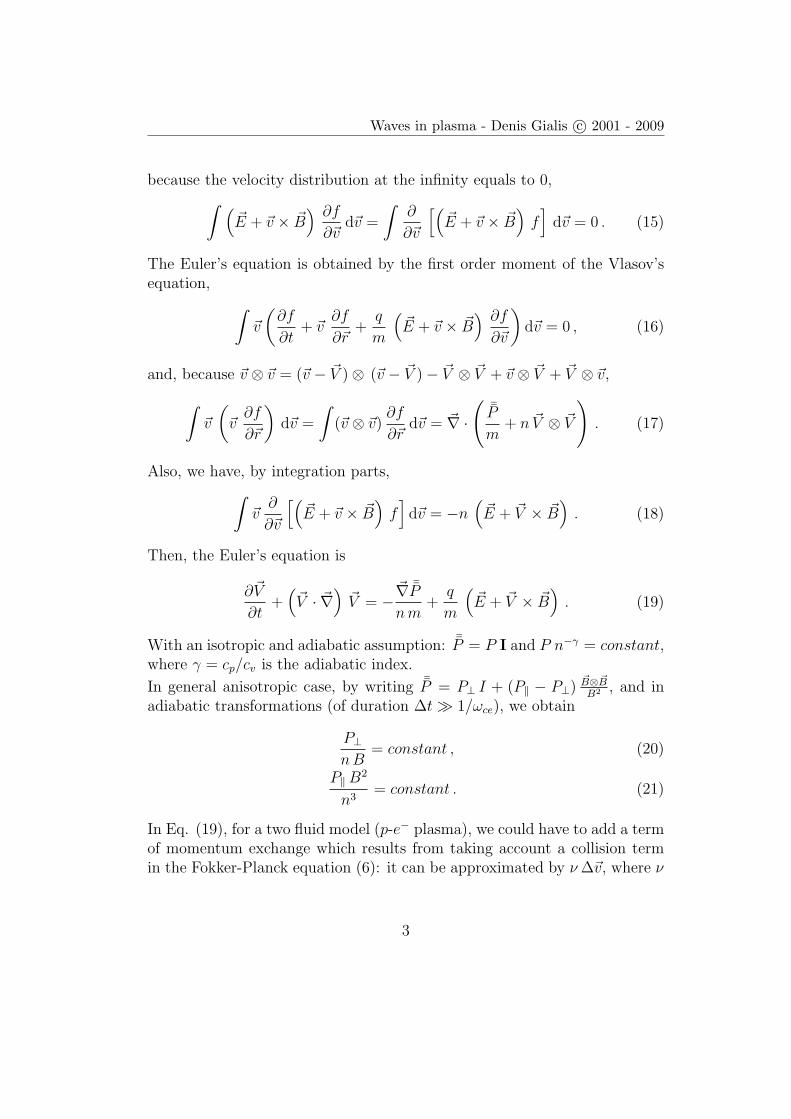
because the velocity distribution at the infinity equals to 0,

∫ (~E + ~v × ~B

) ∂f

∂~vd~v =

∫∂

∂~v

[(~E + ~v × ~B

)f]

d~v = 0 . (15)

The Euler’s equation is obtained by the first order moment of the Vlasov’sequation,

∫~v

(∂f

∂t+ ~v

∂f

∂~r+

q

m

(~E + ~v × ~B

) ∂f

∂~v

)d~v = 0 , (16)

and, because ~v ⊗ ~v = (~v − ~V )⊗ (~v − ~V )− ~V ⊗ ~V + ~v ⊗ ~V + ~V ⊗ ~v,

∫~v

(~v

∂f

∂~r

)d~v =

∫(~v ⊗ ~v)

∂f

∂~rd~v = ~∇ ·

(¯P

m+ n ~V ⊗ ~V

). (17)

Also, we have, by integration parts,

∫~v

∂

∂~v

[(~E + ~v × ~B

)f]d~v = −n

(~E + ~V × ~B

). (18)

Then, the Euler’s equation is

∂~V

∂t+

(~V · ~∇

)~V = −

~∇ ¯P

nm+

q

m

(~E + ~V × ~B

). (19)

With an isotropic and adiabatic assumption: ¯P = P I and P n−γ = constant,where γ = cp/cv is the adiabatic index.

In general anisotropic case, by writing ¯P = P⊥ I + (P‖ − P⊥)~B⊗ ~BB2 , and in

adiabatic transformations (of duration ∆t À 1/ωce), we obtain

P⊥nB

= constant , (20)

P‖ B2

n3= constant . (21)

In Eq. (19), for a two fluid model (p-e− plasma), we could have to add a termof momentum exchange which results from taking account a collision termin the Fokker-Planck equation (6): it can be approximated by ν ∆~v, where ν

3


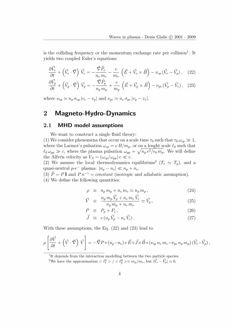
is the colliding frequency or the momentum exchange rate per collision1. Ityields two coupled Euler’s equations:

∂~Ve

∂t+

(~Ve · ~∇

)~Ve = −

~∇ ¯Pe

ne me

− e

me

(~E + ~Ve × ~B

)− νep (~Ve − ~Vp) , (22)

∂~Vp

∂t+

(~Vp · ~∇

)~Vp = −

~∇ ¯Pp

np mp

+e

mp

(~E + ~Vp × ~B

)− νpe (~Vp − ~Ve) , (23)

where νep ' np σep |ve − vp| and νpe ' ne σpe |vp − ve|.

2 Magneto-Hydro-Dynamics

2.1 MHD model assumptions

We want to construct a single fluid theory:(1) We consider phenomena that occur on a scale time τ0 such that τ0 ωcp À 1,where the Larmor’s pulsation ωcp = eB/mp, or on a lenght scale `0 such that`0 ωpp À c, where the plasma pulsation ωpp =

√np e2/ε0 mp. We will define

the Alfven velocity as VA = (ωcp/ωpp) c ¿ c.(2) We assume the local thermodynamics equilibrium2 (Te ' Tp), and aquasi-neutral p-e− plasma: |np − ne| ¿ np + ne.

(3) ¯P = P I and P n−γ = constant (isotropic and adiabatic assumption).(4) We define the following quantities:

ρ ≡ np mp + ne me ' np mp , (24)

~V ≡ np mp~Vp + ne me

~Ve

np mp + ne me

' ~Vp , (25)

P ≡ Pp + Pe , (26)

~J ≡ e (np~Vp − ne

~Ve) . (27)

With these assumptions, the Eq. (22) and (23) lead to

ρ

[∂~V

∂t+

(~V · ~∇

)~V

]= −~∇P+(np−ne) e ~E+ ~J× ~B+(νep ne me−νpe np mp) (~Ve−~Vp) ,

1It depends from the interaction modelling between the two particle species.2We have the approximation < ~v2

e > / < ~v2p >' mp/me, but |~Ve − ~Vp| ' 0.

4


or, taking into account the quasi-neutrality assumption and equality in mo-mentum exchange (ne meνep = np mp νpe or νep = (mp/me) νpe),

ρ

[∂~V

∂t+

(~V · ~∇

)~V

]= −~∇P + ~J × ~B . (28)

Also, because ~Ve = ~Vp − ~J/e ne ' ~V − ~J/e ne, we deduce from Eq. (22) that

~E + ~V × ~B − me ν

ne e2~J −

~J × ~B

ne e= 0 , (29)

by neglecting d~Ve/dt and ~∇Pe in the fluid model, and with ν = νep.

With η ≡ ne e2

me ν(Spitzer conductivity), ωce ≡ eB/me and ~b = ~B/B, the

generalized Ohm law is written

~J +ωce

ν

(~J ×~b

)= η

(~E + ~V × ~B

). (30)

The current density vector, with ~E‖ = ( ~E ·~b)~b and ~E⊥ = ~b× ( ~E×~b), can beeasily expressed

~J = η ~E‖ + η⊥(

~E⊥ + ~V × ~B)

+ η×~b×(

~E⊥ + ~V × ~B)

, (31)

where η⊥ = η/(1 + ω2c/ν

2) and η× = η/(ν/ωc + ωc/ν).

There are two asymptotic limits:

(1) When ωce ¿ ν, the Ohm’s law becomes isotropic and ~J = η(

~E + ~V × ~B).

This is the “resistive” MHD regime.(2) When the plasma is collisionless, i.e ν → 0 (or η → +∞), with a finite ra-tio ωce/ν, we have the approximation of the “ideal MHD” or the non-resistive

MHD regime: ~E + ~V × ~B = 0. But, when | ~J × ~B|/e ne |~V × ~B| ¿ 1, we

have also ~J = η(

~E + ~V × ~B): this is the case when `0 ωpp À c (first MHD

assumption) and V0 ∼ `0/τ0 6= 0. Otherwise it is necessary to have ωce ¿ ν.

When the electromagnetic field is slightly variable (over scales `0 and τ0),

|~∇× ~E| ∼ E0/`0 ∼ B0/τ0, |∂ ~E/∂t| ∼ E0/τ0 and |~∇× ~B| ∼ B0/`0, where E0

and B0 are the characteristic values of E and B. Thus we have

|(1/c2) ∂ ~E/∂t||~∇× ~B|

∼ (`0/τ0)2

c2¿ 1 , (32)

5


in the non-relativistic MHD regime, and the Eq. (4) becomes ~∇× ~B = µ0~J .

Assuming an isotropic Ohm’s law, we deduce from Eq. (3) and (4),

∂ ~B

∂t− ~∇× (~V × ~B) = νm ∆ ~B , (33)

where νm = 1/µ0 η is the magnetic diffusivity. We can form the ratio betweenthe advective and the diffusive terms

|~∇× (~V × ~B)||νm ∆ ~B|

∼ V0 B0/`0

νm B0/`20

=V0 `0

νm

, (34)

where V0 (¿ c) is the characteristic velocity (∼ VA) of the MHD fluid. Thisratio is defined as the magnetic Reynold number Rm. When Rm . 1, theplasma dynamics is dominated by its resistivity and its diffusion. WhenRm À 1, this is the ideal MHD regime: the diffusion can be neglected and,the magnetic field and the MHD fluid are “frozen” together.

2.2 Ideal MHD and waves

According to the previous section, the ideal MHD equations are:

∂ρ

∂t= −~∇

(ρ ~V

), (35)

∂ ~B

∂t= ~∇× (~V × ~B) , (36)

d

dt

(P ρ−γ

)= 0 , (37)

ρ

[∂~V

∂t+

(~V · ~∇

)~V

]= −~∇P +

~∇× ~B

µ0

× ~B . (38)

In the Eq. (38), the term (~∇× ~B)× ~B can be written ( ~B · ~∇) ~B− (1/2) ~∇B2.Thus, we have

ρ

[∂~V

∂t+

(~V · ~∇

)~V

]= −~∇P − ~∇Pm + ~Tm , (39)

where the magnetic pressure Pm ≡ B2/2µ0, and the magnetic tension, ~Tm, issuch that

~Tm ≡ ( ~B · ~∇) ~B

µ0

=d

ds

(B2

2µ0

)~b +

B2

µ0

~b⊥Rc

, (40)

6


where s is the curvilinear abscissa, ~b⊥ is the unit vector perpendicular to~b = ~B/B, and Rc, the curvature radius of the magnetic field line. Thus, theLaplace’s force (per unit of volum) can be written

~fL = ~J × ~B = −~∇⊥Pm +2Pm

Rc

~b⊥ . (41)

If P/Pm < 1, the plasma undergoes the magnetic dynamics, and if P/Pm > 1,the magnetic field undergoes the plasma dynamics.At last, the Eq. (37) can be transformed

∂P

∂t= −~v ~∇P − γ P ~∇~v . (42)

Let us study the effects of a weak perturbation. The linearization process isthe following one: considering a Fourier decomposition, all complex quanti-ties X will be such that X = X0+x where X0 is a real time invariant quantityand |x/X0| ¿ 1. The perturbative quantity x will be ∝ exp[i (ω t − ~k · ~r)](where i2 = −1). The only condition on the pulsation ω is that ω ¿ ωcp.

Thus, we will have ∂/∂t ≡ i ω, ~∇· ≡ −i~k, ~∇× ≡ −i~k× and ~∇2 ≡ −k2,when one derive these perturbative quantities (only).

Assuming that ~V0 = ~0 and writing ρ = ρ0 + δρ, the Eqs. (35) to (38) yield

δρ =ρ0

ω~k · ~v , (43)

~b = − 1

ω~k × (~v × ~B0) , (44)

iω p = −~v ~∇P0 + iγ P0~k · ~v , (45)

iω ρ0 ~v = −~∇[p +

~B0 ·~bµ0

]+

1

µ0

[( ~B0 · ~∇)~b + (~b · ~∇) ~B0

]. (46)

In fact, the Eq. (46) is obtained because, following the Eq. (39), we have

~∇P0 = −~∇(

B20

2µ0

)+

( ~B0 · ~∇) ~B0

µ0

. (47)

7


2.3 Example: MHD waves in homogeneous medium

We consider here a simple case: the medium is homogeneous i.e the spatialvariation of quantities X0 are negligible. The Eqs. (45) and (46) yield

ω p = γ P0~k · ~v , (48)

ω ρ0 ~v = p~k +1

µ0

~B0 ×(~k ×~b

). (49)

With the Eq. (44), we obtain

ω2 ρ0 ~v = γ P0

(~k · ~v

)~k − 1

µ0

~B0 ×[~k ×

(~k ×

(~v × ~B0

))]. (50)

Let us define the basis vectors ~e‖ = ~B0/| ~B0|, ~e⊥ = ~k⊥/|~k⊥| when |~k⊥| 6= 0(otherwise ~e⊥ is an arbitrary perpendicular unit vector), and ~e× = ~e‖ × ~e⊥,

with ~k = k‖ ~e‖ + k⊥ ~e⊥ and ~v = v‖ ~e‖ + v⊥ ~e⊥ + v× ~e×. We will have

− 1

µ0

~B0 ×[~k ×

(~k ×

(~v × ~B0

))]=

1

µ0

B20

(v⊥ k2 ~e⊥ + v× k2

‖ ~e×)

. (51)

Thus, the Eq. (50) leads to the system

(ω2 − C2

s k2‖)

v‖ − C2s k‖ k⊥ v⊥ = 0 , (52)(

ω2 − C2s k2

⊥ − V 2A k2

)v⊥ − C2

s k‖ k⊥ v‖ = 0 , (53)(ω2 − V 2

A k2‖)

v× = 0 , (54)

with the sound velocity Cs =√

γ P0/ρ0 and the Alfven velocity VA =√B2

0/(ρ0µ0) for (B20/µ0)/ρ0 c2 ¿ 1. In its matricial form, this system be-

comes

(ω2 − C2s k2

‖) −C2s k‖ k⊥ 0

−C2s k‖ k⊥ (ω2 − C2

s k2⊥ − V 2

A k2) 00 0 (ω2 − V 2

A k2‖)

v‖v⊥v×

= 0 . (55)

The solutions of this system (proper modes) are determined by det = 0. TheAlfven waves are then defined by the following dispersion relation,

ω2 = V 2A k2

‖ , (56)

8


and the fast (+) and slow (−) magnetosonic waves are determined by thedispersion relation,

ω2f,s =

k2

2

(C2

s + V 2A)±

√(C2

s + V 2A)2 − 4 C2

s V2A

(k‖k

)2 . (57)

3 Electromagnetic waves in fluid model

3.1 Assumptions

In the Sec. 3, we will consider the following assumptions:

General assumption of adiabaticity:(1) The phase velocity of waves, vφ = ω/k, is supposed to be À vth, thethermal velocity of charged particle species.(2) The energy density of the EM waves is ¿ the thermal energy density.(3) The damping of EM waves is neglected.(4) The collision effects are neglected: ν → 0.

Additional assumption: the plasma is homogeneous.

We will define:The plasma pulsation of the species a: ωpa =

√na q2

a/ε0 ma, where na, qa

and ma, are respectively the density, the charge and the mass of a.The cyclotronic or Larmor pulsation of the species a: ωca = |qa|B0/ma,where B0 is the intensity of the magnetic field.

3.2 Electromagnetic mode

The plasma is assumed to be isotropic and unmagnetized (B0 = 0).

We first neglect the ionic response ( ~Jp) and the temperature (Te = Tp ' 0).With the previous assumptions, the Eq. (22) leads to

∂~Ve

∂t+

(~Ve · ~∇

)~Ve = − e

me

(~E + ~Ve × ~B

). (58)

9


The fields ~E and ~B are considered as perturbations. Following the lineariza-tion process, as explained in Sec. 2.2, the Eq. (58) simply becomes

∂~Ve

∂t= − e

me

~E , (59)

and, because ~Je = ne e ~Ve, we obtain

~Je = −iω2

pe

ωε0

~E . (60)

Thus, the Eqs. (3) and (4) could be written

~k × ~E = ω ~B , (61)

~k × ~B = i ~Je − ω ε0~E , (62)

and we deduce (~k · ~E

)~k − k2 ~E =

ω2pe − ω2

c2~E . (63)

For the electromagnetic mode (~k · ~E = 0), this equation yields the followingdispersion relation:

ω2 = ω2pe + k2 c2 . (64)

For ω > ωpe, the phase velocity ω/k is superluminal and the EM wave wellverifies the assumption of adiabaticity. For ω < ωpe, the EM wave is evanes-cent.

For ~k × ~E = ~0, we obtain the plasmon mode ω = ωpe, but with no energytransport. It corresponds to Langmuir’s oscillations.

3.3 Bohm-Gross and ionic acoustic modes

The plasma is assumed to be isotropic and unmagnetized (B0 = 0).

We neglect the ionic response ( ~Jp ' ~0) and the ionic temperature (Tp ' 0).With these assumptions, the Eq. (22) leads to

∂~Ve

∂t+

(~Ve · ~∇

)~Ve = −

~∇Pe

ne me

− e

me

(~E + ~Ve × ~B

), (65)

10


and we suppose the isentropic state equation (37). According to the lin-earization process and the continuity equation (giving the Eq. (42)), weobtain first

p =γ

ωPe

~k · ~Ve , (66)

with Pe = ne kB Te, where kB is the Boltzmann constant. Thus, the Eq. (65)can be written

~Je = −iω2

pe

ωε0

~E +γ kB Te

me ω2

(~k · ~Je

)~k. (67)

For ~k × ~E = ~0, we obtain the Bohm-Gross mode: indeed, because of theprevious equation, ~k × ~Je = ~0, and we have

~Je = −iω2

pe

ω

ε0~E

1− γ kB Te k2

me ω2

. (68)

The dispersion relation of the Bohm-Gross mode is thus

ω2 = ω2pe +

γ kB Te

me

k2 . (69)

For ω < ωpe, there is no pure electronic mode. We have to take into accountthe ionic dynamics. We first assume low frequencies such that

kB Tp

mp

<ω2

k2<

kB Te

me

. (70)

This is at the limit of the first adiabatic assumption (see Sec. 3.1). Weneglect the electronic inertia. The Eq. (68) gives

~Je ' −i ω2pe

me ω ε0~E

γ kB Te k2. (71)

Concerning the ionic current, the Eq. (23) (with Tp ' 0) and the linearizationprocess lead to

~Jp = −iω2

pp

ωε0

~E . (72)

For low frequencies ω ¿ ωpp, one can assume the quasi-neutrality of current:~Je + ~Jp ' ~0. Indeed, because ~∇× ~B = 0, we have ~Je + ~Jp + i ω ε0

~E = ~0 and

|ω ε0~E|

| ~Je + ~Jp|' ω2

ω2pp

[1− me ω2

pe

γ kB Te k2

ω2

ω2pp

+ o

(ω2

ω2pp

)]. (73)

11


We then deduce the following dispersion relation for the phonon mode;

ω = Cs k , (74)

with Cs =√

γ kB Te/mp.

For higher frequencies such that ωpp > ω > k√

kB Te/me, we cannot assumethe quasi-neutrality. The Eqs. (68) and (72) yield

ω2pp

ω2+

ω2pp

(me/mp)ω2 − k2 C2s

= 1 , (75)

with ωpp/ωpe =√

me/mp. By neglecting the term (me/mp)ω2, we obtain the

dispersion relation of the ionic acoustic mode;

ω ' ωppCs k√

ω2pp + C2

s k2. (76)

In this mode, we cannot have ω2pp ¿ C2

s k2 which leads to ω ' ωpp, because

the condition ω/k À √kB Te/mp would not be satisfied and we would have

to take into account Landau’s damping.

3.4 Magnetized electronic and ionic modes

The plasma is assumed to be magnetized. We will define the basis{~e‖, ~e⊥, ~e×} as described in Sec. 2.3.

3.4.1 Electronic modes

We first neglect the ionic response ( ~Jp ' ~0) and the temperature (Te =Tp ' 0). With these assumptions, the Eq. (22) leads to

∂~Ve

∂t+

(~Ve · ~∇

)~Ve = − e

me

(~E + ~Ve × ~B

), (77)

and the linearization process yields

~Je = −iω2

pe

ωε0

~E + iωce

ω~Je × ~e‖ . (78)

12


Because

~Je · ~e‖ = −iω2

pe

ωε0

~E · ~e‖ , (79)

~Je × ~e‖ = −iω2

pe

ωε0

~E × ~e‖ − iωce

ω~Je + i

ωce

ω

(~Je · ~e‖

)~e‖ , (80)

we deduce

~Je = −iω2

pe ω

ω2 − ω2ce

[ε0

~E + iωce

ωε0

~E × ~e‖ − ω2ce

ω2ε0

(~E · ~e‖

)~e‖

]. (81)

The Eqs. (3) and (4) gives

~k ×(~k × ~E

)+

ω2

c2

[ε⊥(ω) ~E +

ωce

ωε×(ω)

(~E · ~e‖

)~e‖ − i ε×(ω) ~E × ~e‖

]= ~0

(82)with the coefficients,

ε⊥(ω) = 1− ω2pe

ω2 − ω2ce

, (83)

ε×(ω) =ωce

ω

ω2pe

ω2 − ω2ce

. (84)

By defining ~E = ~E‖ + ~E⊥ with ~E‖ = E‖ ~e‖ and ~E⊥ · ~e‖ = 0, we obtain

~k ×(~k × ~E

)+

ω2

c2

[ε‖(ω) ~E‖ + ε⊥(ω) ~E⊥ − i ε×(ω) ~E⊥ × ~e‖

]= ~0 , (85)

with the last coefficient,

ε‖(ω) = 1− ω2pe

ω2. (86)

(1) For a parallel propagation i.e ~k = k‖ ~e‖, the Eq. (85) is equivalent to

ω2

c2ε‖ 0 0

0 ω2

c2ε⊥ − k2

‖ −i ω2

c2ε×

0 i ω2

c2ε× ω2

c2ε⊥ − k2

‖

E‖E⊥y

E⊥z

= 0 , (87)

13


in the basis {~e‖, ~e⊥, ~e×}. For ~E = ~E‖, we recognize the plasmon mode (see

Sec. 3.2) with ω = ωpe. For ~E 6= ~E‖, the other proper modes are obtainedfor det = 0 i.e k2

‖ c2 = ω2 (ε⊥ ± ε×). The two dispersion relations correspondto the following modes:

(1-a) The left mode (L-mode):

k2‖ =

ω2

c2

[1− ω2

pe

ω (ω + ωce)

], (88)

with the cut-off frequency (k‖ = 0) such that

ωL =

√ω2

pe +ω2

ce

4− ωce

2. (89)

(1-b) The right mode (R-mode):

k2‖ =

ω2

c2

[1− ω2

pe

ω (ω − ωce)

], (90)


ωR =

√ω2

pe +ω2

ce

4+

ωce

2, (91)

and the resonance frequency (k‖ → +∞) for ω → ωce.We can plot two different Brillouin diagrams (ω-k plane) for the R-mode: fora strong magnetized plasma, ωce > ωpe, and for a dense plasma, ωce < ωpe.

The different phase velocity between the R-mode and the L-mode is at theorigin of the Faraday effect, for a rectilinear polarized wave, which is therotation of the rectilinear polarization plane.

For ω ¿ ωce, the R-mode is named whistler mode and the dispersion relationis simply:

ω = k2‖ c2 ωce

ω2pe

. (92)

The group velocity is thus vg = ∂ω/∂k‖ ∝√

ω.

14


(2) For a perpendicular propagation i.e, for example, ~k = k⊥ ~e⊥, the Eq.(85) is equivalent to

ω2

c2ε‖ − k2

⊥ 0 0

0 ω2

c2ε⊥ −i ω2

c2ε×

0 i ω2

c2ε× ω2

c2ε⊥ − k2

⊥

E‖E⊥y

E⊥z

= 0 , (93)

in the basis {~e‖, ~e⊥, ~e×}. For ~E⊥ = ~0, we obtain the ordinary mode with thedispersion relation:

ω2 = ω2pe + k2

⊥ c2 . (94)

This is similar to the electromagnetic mode previously obtained in Sec. 3.2.For ~E⊥ 6= ~0, we deduce from det = 0, the extraordinary mode with thefollowing dispersion relation:

k2⊥ c2 = ω2 (ε⊥ − ε2

×/ε⊥) , (95)

which can be written

k2⊥ c2 =

(ω2 − ω2R) (ω2 − ω2

L)

ω2 − ω2UH

, (96)

where the frequency of the high hybrid resonance, corresponding to the Lang-muir electronic oscillation, is such that

ω2UH =

1

2

[ω2

ce + ω2pe +

√ω2

ce + ω2pe − 4 ω2

ce (ω2cp + ω2

pp)]

. (97)

For ωpe À ωpp and, because ωce À ωcp, ωUH ' √ω2

ce + ω2pe.

(3) For an oblique propagation, ~k = k⊥ ~e⊥ + k‖ ~e‖, with k⊥ = k sin θ andk‖ = k cos θ. The Eq. (85) is equivalent to

ω2

c2ε‖ − k2

⊥ 0 k⊥ k‖0 ω2

c2ε⊥ − k2

‖ − k2⊥ −i ω2

c2ε×

k⊥ k‖ i ω2

c2ε× ω2

c2ε⊥ − k2

‖

E‖E⊥y

E⊥z

= 0 , (98)

in the basis {~e‖, ~e⊥, ~e×}. By defining,

a1(θ) = ε⊥ sin2 θ + ε‖ cos2 θ , (99)

a2(θ) = ε⊥ ε‖ (1 + cos2 θ) + (ε2⊥ − ε2

×) sin2 θ , (100)

a3 = ε‖ (ε2⊥ − ε2

×) , (101)

15


we obtain the proper modes (det = 0) with the equation

a1

(k c

ω

)4

− a2

(k c

ω

)2

+ a3 = 0 . (102)

Thus, we have the dispersion relation

k =ω

c

√a2 ±

√a2

2 − 4a1 a3

2a1

. (103)

There are resonances (k → +∞) for a1 → 0 and cut-off (k → 0) for a3 → 0.

3.4.2 Ionic modes

We also consider a cold plasma by neglecting the temperature (Te = Tp '0), but we introduce the ionic current ( ~Jp 6= ~0). With these assumptions, theEqs. (22) and (23), and the linearization process, yield

~Je = −iω2

pe ω

ω2 − ω2ce

[ε0

~E + iωce

ωε0

~E × ~e‖ − ω2ce

ω2ε0

(~E · ~e‖

)~e‖

], (104)

~Jp = −iω2

pp ω

ω2 − ω2cp

[ε0

~E − iωcp

ωε0

~E × ~e‖ −ω2

cp

ω2ε0

(~E · ~e‖

)~e‖

], (105)

and we obtain the same relation than in the previous section,

~k ×(~k × ~E

)+

ω2

c2

[ε‖(ω) ~E‖ + ε⊥(ω) ~E⊥ − i ε×(ω) ~E⊥ × ~e‖

]= ~0 , (106)

but with the following new definitions for coefficients

ε⊥(ω) = 1− ω2pe

ω2 − ω2ce

− ω2pp

ω2 − ω2cp

, (107)

ε×(ω) =ωce

ω

ω2pe

ω2 − ω2ce

− ωcp

ω

ω2pp

ω2 − ω2cp

, (108)

ε‖(ω) = 1− ω2pe

ω2− ω2

pp

ω2. (109)

For high frequencies (ω À ωcp), the situation is the same one than in theSec. 3.4.1.

16


For very low frequencies (ω → 0), because ωce À ωcp, we have ε‖ → −ω2pe/ω,

ε⊥ → 1 + c2/V 2A and, ε× → (c2/V 2

A) ω/ωcp.

(1) For a parallel propagation i.e ~k = k‖ ~e‖, and for ~E 6= ~E‖, the Eq. (106)leads to k2

‖ c2 = ω2 (ε⊥± ε×). For low frequencies (ω ¿ ωpp), and for ne ' np

(i.e ω2pp/ωcp ' ω2

pe/ωce), we deduce

ω2 = k2‖ V 2

A

[1± ω

ωcp

+ o

(ω

ωcp

)]. (110)

We thus define again the following modes:

(1-a) The left mode (L-mode):

ω ' k‖ VA

√1− ω

ωcp

. (111)

(1-b) The right mode (R-mode):

ω ' k‖ VA

√1 +

ω

ωcp

. (112)

For ω → 0, these two modes blend into the Alfven mode, as previously de-scribed in Sec. 2.3: ω ' k‖ VA.

(2) For a perpendicular propagation i.e, for example, ~k = k⊥ ~e⊥, and

for ~E⊥ 6= ~0, we deduce from the Eq. (106) the dispersion relation for theextraordinary mode:

k2⊥ c2 = ω2 (ε⊥ − ε2

×/ε⊥) , (113)

which leads to

k2⊥ c2 = ω2 (ω2 − ω2

R) (ω2 − ω2L)

(ω2 − ω2LH)(ω2 − ω2

UH), (114)

where the frequency of the low hybrid resonance, corresponding to the Lang-muir oscillation, is such that

ω2LH =

1

2

[ω2

ce + ω2pe −

√ω2

ce + ω2pe − 4 ω2

ce (ω2cp + ω2

pp)]

. (115)

For ωpe À ωpp and, because ωce À ωcp, we have

ωLH ' ωce

√ω2

cp + ω2pp

ω2ce + ω2

pe

' √ωce ωcp. (116)

17


For ω → 0, we recognize again the Alfven mode because ω ' k⊥ VA/√

1 + V 2A/c2 '

k⊥ VA (with VA ¿ c).

(3) If we slightly modify the assumptions by taking into account theelectronic compressibility effects (Te 6= 0), and if we consider pulsations ωsuch that ωcp < ω < ωce, the modification of the Eq. (104) with the pressureterm, and the Eq. (105) give

~Je‖ ' −iω2

pe

ωε0

~E‖ +γ kB Te k2

me ω2~Je‖ , (117)

~Jp‖ ' −iω2

pp ω

ω2 − ω2cp

ε0~E‖ , (118)

with ω2ce/ω

2 À 1 and, by neglecting terms in ωcp/ω. Because ω/k ¿√γ kB Te/me, the Eq. (117) can be written

~Je‖ ' iω2

pe ω me

γ kB Te k2ε0

~E‖ . (119)

The quasi-neutrality of current, ~Je‖ + ~Jp‖ = ~0, leads to dispersion relation ofthe ionic cyclotron mode;

ω2 = ω2cp + C2

s k2 , (120)

with Cs =√

γ kB Te/mp, and because ω2pp/ω

2pe = me/mp.

18


4 Summary

Let us summarize the previous results concerning waves propagating inan isotropic p− e− plasma.

I - For an unmagnetized plasma i.e B0 = 0

I-1 The ionic response ( ~Jp) and the temperature (Te = Tp ' 0) are ne-glected:

- The electromagnetic mode (~k · ~E = 0):

ω2 = ω2pe + k2 c2 . (121)

For ω > ωpe, the phase velocity ω/k is superluminal.For ω < ωpe, the EM wave is evanescent (k = kr + i ki, with ki 6= 0).

- The plasmon mode or Langmuir’s oscillations (~k × ~E = ~0):ω = ωpe. No energy transport.

I-2 The ionic response ( ~Jp) and the ionic temperature (Tp ' 0) are firstneglected:

- The Bohm-Gross mode (~k × ~E = ~0):

ω2 = ω2pe +

γ kB Te

me

k2 . (122)

For ω < ωpe, there is no pure electronic mode. We have to take into account

the ionic dynamics ( ~Jp).

- The phonon mode (ω ¿ ωpp and ~Je + ~Jp ' ~0):

ω = Cs k , (123)

with Cs =√

γ kB Te/mp.

- The ionic acoustic mode (k√

kB Te/me < ω < ωpp):

ω ' ωppCs k√

ω2pp + C2

s k2. (124)

19


II - For a magnetized plasma i.e B0 6= 0

II-1 The electronic modes ( ~Jp ' ~0 and Te = Tp ' 0):

- The L-mode (~k ‖ ~B):

k2‖ =

ω2

c2

[1− ω2

pe

ω (ω + ωce)

], (125)


ωL =

√ω2

pe +ω2

ce

4− ωce

2. (126)

- The R-mode (~k ‖ ~B):

k2‖ =

ω2

c2

[1− ω2

pe

ω (ω − ωce)

], (127)


ωR =

√ω2

pe +ω2

ce

4+

ωce

2, (128)

and the resonance frequency (k‖ → +∞) for ω → ωce.For ω ¿ ωce, the R-mode is named whistler mode and the dispersionrelation is simply:

ω = k2‖ c2 ωce

ω2pe

. (129)

- The ordinary mode equivalent to the electromagnetic mode ( ~E⊥ = ~0

and ~k⊥ ~B):ω2 = ω2

pe + k2⊥ c2 . (130)

- The extraordinary mode ( ~E⊥ 6= ~0 and ~k⊥ ~B):

k2⊥ c2 =

(ω2 − ω2R) (ω2 − ω2

L)

ω2 − ω2UH

, (131)

with the frequency of the high hybrid resonance,

ω2UH =

1

2

[ω2

ce + ω2pe +

√ω2

ce + ω2pe − 4 ω2

ce (ω2cp + ω2

pp)]

. (132)

20


For ωpe À ωpp, ωUH ' √ω2

ce + ω2pe.

II-2 The ionic modes ( ~Jp 6= ~0 and Te = Tp ' 0):

- The L-mode (~k ‖ ~B):

ω ' k‖ VA

√1− ω

ωcp

. (133)

- The R-mode (~k ‖ ~B):

ω ' k‖ VA

√1 +

ω

ωcp

. (134)

For ω → 0, these two modes blend into the Alfven mode: ω ' k‖ VA.

- The extraordinary mode ( ~E⊥ 6= ~0 and ~k⊥ ~B):

k2⊥ c2 = ω2 (ω2 − ω2

R) (ω2 − ω2L)

(ω2 − ω2LH)(ω2 − ω2

UH), (135)

with the frequency of the low hybrid resonance,

ω2LH =

1

2

[ω2

ce + ω2pe −

√ω2

ce + ω2pe − 4 ω2

ce (ω2cp + ω2

pp)]

. (136)

For ωpe À ωpp and, because ωce À ωcp, we have

ωLH ' ωce

√ω2

cp + ω2pp

ω2ce + ω2

pe

' √ωce ωcp. (137)

For ω → 0 (or ω ¿ ωcp), we obtain the Alfven mode because ω ' k⊥ VA/√

1 + V 2A/c2 '

k⊥ VA (with VA ¿ c).

- The slow (-) and fast (+) magnetosonic modes (ω ¿ ωcp):

ω2f,s =

k2

2

(C2

s + V 2A)±

√(C2

s + V 2A)2 − 4 C2

s V2A

(k‖k

)2 . (138)

21

Documents

Waves in plasma - astrosurf.com