Embed Size (px)
Citation preview
Commun. Comput. Phys.doi: 10.4208/cicp.OA-2016-0091
Vol. 21, No. 4, pp. 947-980April 2017
Recovering the Damping Rates of Cyclotron Damped
Plasma Waves from Simulation Data
Cedric Schreiner1,2,∗, Patrick Kilian1 and Felix Spanier1
1 Centre for Space Research, North-West University, Potchefstroom 2520,South Africa.2 Lehrstuhl fur Astronomie, Universitat Wurzburg, 97074 Wurzburg, Germany.
Received 21 June 2016; Accepted (in revised version) 19 September 2016
Abstract. Plasma waves with frequencies close to the particular gyrofrequencies ofthe charged particles in the plasma lose energy due to cyclotron damping. We brieflydiscuss the gyro-resonance of low frequency plasma waves and ions particularly withregard to particle-in-cell (PiC) simulations. A setup is outlined which uses artificiallyexcited waves in the damped regime of the wave mode’s dispersion relation to trackthe damping of the wave’s electromagnetic fields. Extracting the damping rate directlyfrom the field data in real or Fourier space is an intricate and non-trivial task. We there-fore present a simple method of obtaining the damping rate Γ from the simulationdata. This method is described in detail, focusing on a step-by-step explanation of thecourse of actions. In a first application to a test simulation we find that the dampingrates obtained from this simulation generally are in good agreement with theoreticalpredictions. We then compare the results of one-, two- and three-dimensional simula-tion setups and simulations with different physical parameter sets.
AMS subject classifications: 65M75, 65T99, 82C10, 85A30
Key words: Simulation, space physics, plasma, cyclotron resonance, wave damping.
1 Introduction
Turbulence in a magnetized plasma, for example in the solar wind, develops a cascadingspectrum of low frequency waves with ever shorter wave lengths. The spectrum is lim-ited by processes of wave damping, such as Landau damping or the cyclotron resonancefor waves propagating perpendicular or parallel to the magnetic field (or by a mixture ofboth for oblique waves). Since computer simulations of various plasma phenomena and
∗Corresponding author. Email addresses: [email protected] (C. Schreiner),[email protected] (P. Kilian), [email protected] (F. Spanier)
http://www.global-sci.com/ 947 c©2017 Global-Science Press

948 C. Schreiner, P. Kilian and F. Spanier / Commun. Comput. Phys., 21 (2017), pp. 947-980
especially of plasma turbulence are more and more common, it is also interesting to takea closer look at the representation of damping mechanisms in the simulation.
In this article we pick the cyclotron resonance of ions and low frequency waves,i.e. waves with a frequency ω below the cyclotron frequency Ω of the resonating par-ticles. This process can be easily modeled using waves propagating parallel to a back-ground magnetic field and a thermal spectrum of protons. We choose the particle-in-cell(PiC) approach, because it is a self-consistent method which treats kinetic effects in theplasma. Thus, it is expected that a PiC simulation captures cyclotron damping correctly.Of course, PiC is not the only numerical approach which includes cyclotron dampingand other types of code might be used as well to study wave damping.
Determining damping (or growth) rates of plasma waves is not a trivial task. Prop-erties, such as the wave length or wave number, can easily be obtained from looking ata real space representation of the field data or its Fourier transform in space. AnotherFourier transform in time yields frequency information and the dispersion relation ofthe whole wave mode. It is even possible to recover the polarization of single waves orwhole wave modes by adequately combining different components of the electromag-netic fields. However, obtaining the damping rate directly from real or Fourier spaceelectromagnetic field data is challenging.
One approach, though, is to resolve the dispersion relation of the wave mode in ques-tion to such an extend that a broadening in frequency can be observed. For a single wavewith frequency ω0 it may be assumed that the wave’s intensity, represented by its energydensity W, follows a Lorentz profile over frequency ω:
W(ω)=W0 Γ2
(ω−ω0)2+Γ2(1.1)
which is centered around the wave’s frequency ω0 and has a width at half maximum of2Γ, where Γ is the damping rate. Thus, fitting the Lorentz profile from Eq. (1.1) to thedata yields the damping rate of the wave. This is a tedious process and the precisionof the results strongly depends on a high resolution of the frequencies in the dispersionrelation, which is often only achieved by the use of a massive amount of computationalresources.
A simple and fast possibility of studying wave damping (or any other interaction ofwaves and particles) is to analyze the composition of the total energy in the simulation.By comparing the development of the total field energy and the kinetic energy of theparticles – quantities which are often computed during the simulation and saved fordiagnostic purposes – it becomes obvious when and to which extent energy is transferredbetween waves and particles. However, no information about the wave’s properties,such as frequency and wave number, are contained in such a study and several similarprocesses cannot be distinguished. It might even not be possible to tell which wave modeparticipates in the process, especially in fully kinetic simulations which might containseveral possible candidates.
C. Schreiner, P. Kilian and F. Spanier / Commun. Comput. Phys., 21 (2017), pp. 947-980 949
A method to determine the growth rates of different wave modes has been proposedby Koen et al. [1], who study the interaction of three populations of electrons (cold, warmand beam) and electron plasma, acoustic, and beam modes in an electrostatic PiC sim-ulation. Their method is based on the Fourier transformation of field data both in timeand space which is then used to obtain the energy density W(k,ω) as a function of thewave number k and the frequency ω. Thus it is possible to discriminate between differentwaves or wave modes (described by their wave numbers k and corresponding frequen-cies ω). Whereas Koen et al. [1] analyze several wave modes at once and thus need a highresolution in ω to be able to separate the different modes, we will show that such a highresolution is not necessary for their method to work.
In the article at hand, we focus on a step-by-step explanation of the method of [1]and its extension to cyclotron damping. We measure the damping rates of individuallow-frequency L-mode waves undergoing cyclotron damping in an electromagnetic PiCsimulation. On this example we demonstrate that the method can even be applied ifthe spectral resolution is low and the frequency range of the wave mode in questionis not resolved. It is sufficient to distinguish these waves only by their wave number.Furthermore we apply the method to a series of simulations to investigate the quality ofthe representation of cyclotron damping in PiC simulations in different numerical andphysical scenarios.
The article is organized as follows: We first give a brief description of the numericalmethods and the setup of our PiC simulations in Sections 2 and 3. The approach tomeasuring the damping rate is presented in Section 4 and illustrated by its applicationto an example simulation. Studies of the effects of the simulation’s dimensionality, i.e.a one-, two- or three-dimensional setup, and different sets of physical parameters arediscussed in Sections 5 and 6, respectively. Finally, we summarize our results in Section7.
2 Numerical methods and theory
2.1 PiC code
Our PiC simulations are carried out using the ACRONYM code [2], which is designedto employ second-order numerical schemes throughout the code. The ACRONYM codeis an electromagnetic, fully relativistic, explicit PiC code which supports one-, two- orthree-dimensional setups, while electromagnetic fields and particle velocities are alwaystreated as three-dimensional vectors.
Furthermore we use the initial conditions described by [3] to excite one or more wavesat the beginning of the simulation. The excitation mechanism allows for the creation ofdamped waves in the initialization phase. These waves are then damped during thesimulation (“free decay”), losing field energy to the particles. The energy loss can bemeasured and is the basis for our analysis of the damping rate.

950 C. Schreiner, P. Kilian and F. Spanier / Commun. Comput. Phys., 21 (2017), pp. 947-980
2.2 Warm plasma dispersion relation
For later comparison of simulation results and theory we also compute the theoreticaldamping rate from the warm plasma dispersion relation. We follow the notation of [4],who give the generalized dispersion relation D(ωc,k‖) for the parallel propagating, left-handed L-mode [5] in their Eq. (1):
0=D(ωc,k‖)=ω2c −k2
‖ c2+∑s
ω2p,s Is. (2.1)
Here, ωc = ω+ıΓ is the complex frequency, containing the real frequency ω and thegrowth / damping rate Γ of a parallel propagating wave with wave number k‖. Theindex s denotes a particle species (such as electrons or protons), ωp,s is the plasma fre-quency of species s and c is the speed of light. Chen et al. [4] then give a function Is for aMaxwellian particle distribution (with potentially different plasma temperatures paralleland perpendicular to the background magnetic field):
Is=α2⊥s
α2‖s
−1+
(
α2⊥s
α2‖s
ωc∓Ωs
±Ωs+1
)
±Ωs
k‖α‖sZ(ζs), (2.2)
where Z(ζs) is the plasma dispersion function [6] with the argument ζs=(ωc∓Ωs)/(k‖α‖s).The cyclotron frequency Ωs=(qs B0)/(ms c) may have a different sign for different particlespecies, depending on their charge qs. The background magnetic field is denoted by B0
and the particle mass by ms. Normalized thermal velocities in parallel and perpendiculardirection are given by the parameters α‖s and α⊥s, which are defined via the temperature
T‖/⊥=(mα2‖/⊥)/2 (indices for particle species are omitted here).
Our Eq. (2.2) is a slightly modified version of Eq. (13) from [4], where we have in-cluded alternating signs (±). The upper signs are identical to the ones in the originalequation and refer to the L-mode, whereas the lower signs refer to the right-handed, cir-cularly polarized R-mode. Thus, Eq. (2.1) describes both L- and R- mode, depending onthe signs chosen in Eq. (2.2).
The combination of Eqs. (2.1) and (2.2) can be solved numerically and yields the com-plete dispersion relation for the L- or the R-mode in a magnetized, warm plasma. Sincethese wave modes include only parallel propagating waves, the damping rate Γ obtainedfrom the dispersion relation refers to cyclotron damping and can be used to evaluate theresults of our PiC simulations.
3 Simulation setup for example simulations
In this section we describe a simple setup which can be used to analyze cyclotron damp-ing of parallel propagating plasma waves. The setup described is not meant to mirror aspecific real-world counterpart, but is solely chosen for its numerical convenience.

C. Schreiner, P. Kilian and F. Spanier / Commun. Comput. Phys., 21 (2017), pp. 947-980 951
Please note that wave numbers are discretized in a PiC simulation due to the dis-cretization of physical space into individual grid cells. Thus, each wave mode consists ofa limited number of individual waves, which each can be characterized by their specificwave number k and a corresponding frequency. In the following, we refer to an individ-ual oscillation with a wave number k and frequency ω as “a wave”. Each wave mode ina simulation can be decomposed into a countable number of individual waves. With theterm “waves of the L-mode” to refer to the complete set of individual waves which makeup the wave mode.
3.1 Basic setup
In order to obtain the best resolution of the wave and still minimize the computing timewe choose a long but narrow three-dimensional simulation box with periodic boundaryconditions. The background magnetic field is chosen to point in the direction of the longedge of the simulation box. The box length in the long (parallel) direction defines themaximum wave length for any parallel propagating wave and has to be chosen accordingto the desired specifications of the excited waves. The radius of a particle’s undisturbedgyration about the background magnetic field is usually a good indication for the lengthof the two short (perpendicular) edges of the box. Having the short edges be at leasttwice as long as the Larmor radius of a particle traveling with thermal speed allows tocover the full gyration of most particles.
The plasma is characterized by the use of a few parameters: We set the backgroundmagnetic field B0, which fixes the cyclotron frequencies Ωs of the particles. The plasmafrequency of the electrons ωp,e determines the electron density ne. Since we only studyelectron-proton plasmas, the density of the protons is equal to ne and the plasma fre-quency of the protons is then ωp,p = ωp,e
√
me/mp, with the masses of electrons andprotons me and mp. Similarly, the temperature T of the (Maxwellian) plasma is set by
selecting a thermal speed of the electrons vth,e =√
kB Te/me, where kB is the Boltzmannconstant. In the simple case of isotropic temperature (T‖ = T⊥ = T), this translates to
α=2v2th /kB (once again omitting indices for particle species). With Te=Tp=T, the ther-
mal speed of the protons is vth,p=vth,e
√
me/mp. Finally, we choose a mass ratio mp/me,where the electron mass is kept at its natural value, whereas the proton mass can bechanged. To reduce computing time a lower, artificial mass ratio is desirable if protoneffects, such as cyclotron damping of L-mode waves, are to be analyzed.
Physical and numerical parameters used for the example simulation presented in thisarticle can be found in Tables 1 and 2. Additional parameters to the ones discussed aboveare the amplitude of the excited waves, δB, the grid spacing and the length of the timestep, ∆x and ∆t, and the number of time steps, Nt. The size of the simulation box is givenin cells, with N‖ and N⊥ characterizing the directions parallel and perpendicular to the
background magnetic field ~B0.With the start of the simulation, the random thermal motion of the particles cre-
ates electromagnetic fluctuations and eventually all kinds of physically allowed plasma
952 C. Schreiner, P. Kilian and F. Spanier / Commun. Comput. Phys., 21 (2017), pp. 947-980
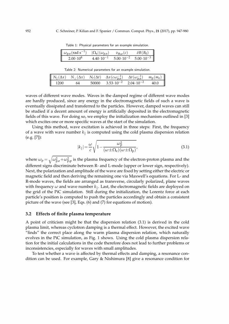
Table 1: Physical parameters for an example simulation.
ωp,e(rad s−1) |Ωe|(ωp,e) vth,e(c) δB(B0)
2.00·108 4.40·10−1 5.00·10−2 5.00·10−3
Table 2: Numerical parameters for an example simulation.
N‖ (∆x) N⊥(∆x) Nt(∆t) ∆x(cω−1p,e) ∆t(ω−1
p,e) mp(me)
1200 64 50000 3.53·10−2 2.04·10−2 40.0
waves of different wave modes. Waves in the damped regime of different wave modesare hardly produced, since any energy in the electromagnetic fields of such a wave iseventually dissipated and transferred to the particles. However, damped waves can stillbe studied if a decent amount of energy is artificially deposited in the electromagneticfields of this wave. For doing so, we employ the initialization mechanism outlined in [3]which excites one or more specific waves at the start of the simulation.
Using this method, wave excitation is achieved in three steps: First, the frequencyof a wave with wave number k‖ is computed using the cold plasma dispersion relation(e.g. [7]):
|k‖|=ω
c
√
1−ω2
p
(ω±Ωe)(ω±Ωp), (3.1)
where ωp =√
ω2p,e+ω2
p,p is the plasma frequency of the electron-proton plasma and the
different signs discriminate between R- and L-mode (upper or lower sign, respectively).Next, the polarization and amplitude of the wave are fixed by setting either the electric ormagnetic field and then deriving the remaining one via Maxwell’s equations. For L- andR-mode waves, the fields are arranged as transverse, circularly polarized, plane waveswith frequency ω and wave number k‖. Last, the electromagnetic fields are deployed onthe grid of the PiC simulation. Still during the initialization, the Lorentz force at eachparticle’s position is computed to push the particles accordingly and obtain a consistentpicture of the wave (see [3], Eqs. (6) and (7) for equations of motion).
3.2 Effects of finite plasma temperature
A point of criticism might be that the dispersion relation (3.1) is derived in the coldplasma limit, whereas cyclotron damping is a thermal effect. However, the excited wave“finds” the correct place along the warm plasma dispersion relation, which naturallyevolves in the PiC simulation, as Fig. 1 shows. Using the cold plasma dispersion rela-tion for the initial calculations in the code therefore does not lead to further problems orinconsistencies, especially for waves with small amplitudes.
To test whether a wave is affected by thermal effects and damping, a resonance con-dition can be used. For example, Gary & Nishimura [8] give a resonance condition for

C. Schreiner, P. Kilian and F. Spanier / Commun. Comput. Phys., 21 (2017), pp. 947-980 953
ω (
|Ωe|)
L mode
R mode
R mode (cold)
ωp
|Ωe|
0
1
2
3
4
5
10-16
10-14
10-12
10-10
10-8
W (
erg
cm
-3)
a)
ω (
|Ωe|)
k|| (|Ωe|/c)
|Ωe| ± 3 √2 k vth,e
|Ωe| ± 3 k vth,e
|Ωe|
0
1
2
3
4
5
-15 -10 -5 0 5 10 15
10-16
10-14
10-12
10-10
10-8
W (
erg
cm
-3)
b)
Figure 1: Dispersion plot obtained from a transverse magnetic field component. The color coded data is thesame in both panels and shows the L- and the R-mode. The dark spot at k‖≈−3c|Ωe|−1 represents an initially
excited wave in the dispersive regime of the R-mode. Solid lines in panel a) are the correct dispersion relationsin a warm plasma, the dashed line shows the result from cold plasma theory. The divergence of the correct(warm) and the approximated (cold) theory becomes obvious as the curves approach |Ωe|. The darker regionsaround k‖=0, ω=|Ωe| which stretch out to larger k‖ can be identified as the regime in which cyclotron damping
becomes important. Panel b) shows the theoretical boundaries of this regime from Eq. (3.2) (left side) and theresult of a modified version of this equation (right side), which seems to be more appropriate.
Landau and cyclotron resonance in their Eqs. (1a) and (1b). For cyclotron damping in aMaxwellian plasma their resonance condition translates to:
ωres,R≥|Ωe|−3√
2k‖vth,e, (3.2)
ωres,L≥Ωp−3√
2k‖vth,p (3.3)
for the R- and L-mode, respectively. In fact, our simulation results suggest similar condi-tions – lacking only the factor of
√2 (see Fig. 1).
4 Obtaining the damping rate
In order to discuss our method of obtaining damping rates from simulation data we setup two simulations using the parameters given in Tables 1 and 2 in Section 3.1. We

954 C. Schreiner, P. Kilian and F. Spanier / Commun. Comput. Phys., 21 (2017), pp. 947-980
choose to excite only waves with odd numerical wave number knum=(k‖ N‖∆x)/(2π) inone of the simulations, and only waves with even knum in the other. This is, of course, notnecessary, but it nicely illustrates the difference between knum with and without excitedwave modes in the dispersion plots (see Fig. 2).
To distinguish between a wave’s physical frequency ω and its apparent frequencyin the dispersion plots obtained from the simulation data, we introduce ωnum. As withthe numerical wave number knum, ωnum is the wave’s frequency measured in pixels orbins in the dispersion plot. Most importantly, for low-frequency waves, whose physicalfrequency ω cannot be resolved due to insufficient spectral resolution of the dispersionplot, the numerical frequency will be ωnum = 0. However, it is worth noting that thewave still propagates (very slowly) during the simulation and that ωnum = 0 does notnecessarily imply |Γ|>ω.
4.1 Dispersion plots
To measure the damping rate of waves on the low frequency branch of the L-mode (orion cyclotron waves) we examine the dispersion plots obtained from our simulations. Asseen in the top panel of Fig. 1, the low frequency regime is usually under-resolved. Thelowest frequency in the dispersion plot is inversely proportional to the total run-time ofthe simulation. To reduce the total number of time steps, the mass ratio is reduced toincrease the proton cyclotron frequency and thus raise the frequencies of all waves onthe low frequency branch of the L-mode. However, this does not mean that the branchwill be resolved in the dispersion plots. Since we are interested in initially excited, butdamped waves, the resolution cannot be improved by increasing the number of timesteps, if the wave in question has already been dissipated until the end of the simulation.
Even if the frequency of the waves can be resolved, there is probably no chance tosee line broadening and to determine the damping rate using a Lorentz profile (1.1) asa fit to the energy density w(ω) as a function of frequency. However, with the methodpresented in this article, we are able to measure the damping rate even if the wave isnot resolved in the dispersion plot, because although the information about the wave’sfrequency is lost, the information about its amplitude remains. This information is storedin the lowest frequency bin (ωnum = 0), but at the correct wave number k and can thusbe easily accessed. By measuring the amplitude (or energy density W) of the wave atmultiple points in time throughout the simulation we are able to model W(t) and obtaina damping rate.
The exact procedure is described in the following and illustrated by Fig. 2. The sim-ulation is split into several intervals with constant length tint (measured in numericalunits ∆t). The data from a specific interval i ∈ 1,2,··· ,Nt/tint can be used to producedispersion relations which characterize the energy distribution in k-ω-space during thisinterval.
In Fig. 2 we present dispersion relations for one transverse component of the mag-netic field along the direction of the background magnetic field ~B0. Panel a) shows the

C. Schreiner, P. Kilian and F. Spanier / Commun. Comput. Phys., 21 (2017), pp. 947-980 955
ω (Ω
p)
L mode
R mode
ωp
|Ωe|
Ωp
0
20
40
60
80
100
10-16
10-14
10-12
10-10
10-8
W (
erg
cm
-3)
a)
ω (Ω
p)
0
20
40
60
80
100
10-16
10-14
10-12
10-10
10-8
W (
erg
cm
-3)
b)
ω (Ω
p)
k|| (Ωp/vA)
0
20
40
60
80
100
-20 -15 -10 -5 0 5 10 15 20
10-16
10-14
10-12
10-10
10-8
W (
erg
cm
-3)
c)
Figure 2: Dispersion relations from one component of the transverse magnetic field along the direction of thebackground magnetic field. The dispersion relation in panel a) contains data from the whole simulation, whereasthe lower panels contain data from a shorter interval at an earlier (b) or later (c) stage of the simulation. Fivewaves have been excited at positive k‖ (dark spots). While wave modes are resolved in a), no single mode
can be seen in b) and c). However, the information about the waves’ amplitudes is still conserved and can beread out. Note that the excited wave modes are symmetric in k because the frequency is under-resolved andinformation about wave propagation is lost. Also note that the broadening of the excited waves in ω has nophysical implications, but is mainly an artifact from using windowing during the Fourier transformation of thedata.
dispersion relation obtained from the data of the entire simulation (i.e. all time steps),whereas the dispersion relations in panels b) and c) were produced at different intervalsin time using only a subset tint of time steps. Compared to panel a) the resolution is con-siderably worse in panels b) and c), but in exchange differences in the intensities of theexcited waves can be observed in the latter panels, representing time evolution. Notethat Fig. 2 shows only excerpts of the complete dispersion plot, since only the region at

956 C. Schreiner, P. Kilian and F. Spanier / Commun. Comput. Phys., 21 (2017), pp. 947-980
small wave numbers and frequencies is relevant. Also note that the total energy densityWtotal (i.e. the sum of the energy densities in all pixels) in the plots is not the same, sincepanel a) yields an average energy density over the course of the whole simulated time,whereas panels b) and c) represent averages over shorter intervals early or late in thesimulation. Due to the transfer of field energy to the particles, the total energy densityWtotal,b in Fig. 2 b) exceeds Wtotal,c in Fig. 2 c). The average over the whole simulation,Wtotal,a, lies somewhere between Wtotal,b and Wtotal,c.
In the case of cyclotron damping, the dispersion relations for each transverse com-ponent of the electric and magnetic fields along the direction of ~B0 have to be computed.Accumulating the energy density at a specific position (knum,ωnum) in each dispersion re-lation gives the total energy density W(ti) of the respective wave during interval i. Notethat ωnum is probably zero, since the frequency is not properly resolved and the wavein question can be entirely characterized by its wave number k. Measuring W in eachinterval yields Nt/tint samples which represent W(t).
4.2 Energy density and damping rate
Summing up the energy densities of all field components for each wave in each inter-val yields the time evolution of the waves’ energy densities (see Fig. 3). We expect theamplitude A of a wave to decay as
A(t)∝ exp(Γt) (4.1)
and thus the energy density to decay as
W(t)∝ A(t)2 ∝ exp(2Γt), (4.2)
where Γ is the damping rate.However, as can be seen from Fig. 3, the energy density does not exhibit the expected
behavior over the course of the whole simulation. An initial phase exists, during whichthe decay proceeds more slowly than expected (i.e. not exponential). The reason for thisnon-exponential onset might lie in the peculiarities of the initialization of the backgroundplasma (excitation of plasma waves by the random motion of thermal particles) or in theprocesses following the excitation of a cold plasma wave which then lead to the estab-lishment of the correct wave in a warm plasma. This initial phase then transits to theexponential decay, which finally comes to a halt when the energy level of the thermalnoise in the background plasma is reached.
Selecting only the data in the exponential phase of wave decay, we then use a leastsquares exponential fit to obtain the damping rate. Depending on the data set, each fitfor a single wave can be based on a different number of data points from the dispersionrelations. The result of the fitting process is presented in Fig. 4 a), where data and fits forten waves from two simulations are shown. In Fig. 4 b) the damping rates Γ(k‖) obtainedfrom the fit functions are plotted over the respective k‖.

C. Schreiner, P. Kilian and F. Spanier / Commun. Comput. Phys., 21 (2017), pp. 947-980 957
10-12
10-11
10-10
10-9
10-8
10-7
10-6
10-5
10-4
0 2 4 6 8 10 12
W (
erg
/ c
m3)
t (1 / Ωp)
w(t, knum=6)
wnoise(knum=6)
Figure 3: Energy density W over time for a single wave with knum =(k‖L‖)/(2π)=6, where L‖ is the length
of the simulation box parallel to the background magnetic field. The dots represent energy measurements fromdispersion relations such as Fig. 2 b) and c). Three intervals of the wave’s evolution can be distinguished: aslow decay until tΩp ≈ 3, exponential decay until tΩp ≈ 7 and random fluctuations after the wave’s energy isbelow the noise limit. The dashed line is the averaged energy density at knum=6 in a simulation without waveexcitation and represents the expected energy level of the background noise.
10-12
10-11
10-10
10-9
10-8
10-7
10-6
10-5
10-4
0 2 4 6 8 10 12
W (
erg
/ c
m3)
t (1 / Ωp)
knum=1
knum=2
knum=3
knum=4
knum=5
knum=6
knum=7
knum=8
knum=9
knum=10
a)
0.0
0.5
1.0
1.5
2.0
2.5
3.0
0 2 4 6 8 10
|Γ| (Ω
p)
k|| (ωpp / c)
theory
data
fit to data
b)
Figure 4: Simulation data and derived damping rates for ten waves with knum=1−10. Panel a) shows the energydensities W of the waves over time. The dashed line is the average of the energy density at knum =1−10 in asimulation without wave excitation. Black solid lines are fitted exponential functions which yield the dampingrate Γ. The obtained damping rates (including statistical errors from the fits) are plotted over k‖ in panel b).
The data can be fitted with the simple fit function from Eq. (4.3) and compared to theoretical predictions fromEqs. (2.1) and (2.2).

958 C. Schreiner, P. Kilian and F. Spanier / Commun. Comput. Phys., 21 (2017), pp. 947-980
To judge the quality of our measurement we compare our results to the predictions ofwarm plasma theory. The theoretical curve Γtheory(k‖) from Eqs. (2.1) and (2.2) is shownin Fig. 4 b). Having used the physical parameters from Table 1 as input parameters forthe PiC simulations and Eqs. (2.1) and (2.2), the measured rates should be in agreementwith Γtheory(k‖) if cyclotron damping is represented correctly in the simulation.
We further employ a fit function to fit our Γ(k‖) [9]:
Γ
Ωp=−m1
(
k‖ c
ωp,p
)m2
·exp
(
−m3
ω2p,p
k2 c2
)
, (4.3)
where m1, m2 and m3 are the fit parameters. This simplistic function yields a qualitativelyand quantitatively accurate approximation of the actual damping rate computed fromwarm plasma theory. For example, if fitted to the theoretical values Γtheory(k‖) at the tendifferent k‖ we chose in the simulations, the full theoretical curve and the fit could hardlybe distinguished in Fig. 4 b) – which is why this fit is not included in the plot.
The more interesting test case is to apply the simple fit function (4.3) to our measure-ment. Fluctuations in the measured data are averaged out in the fit curve, thus givinga better overall representation of Γ over k‖. The newly obtained fit curve can then becompared to theory, or simply be used to interpolate between the points of measureddata.
4.3 Lorentz profiles
We test the method described above against the approach mentioned in Section 1, namelythe description of a wave’s energy distribution W(ω) in frequency space by use of aLorentz profile. For doing so, we first produce dispersion plots and then take the energydensities Wknum
(ωnum) for each knum representing one of the ten waves in the simulationsdiscussed previously. We find that the data is strongly influenced by the number of timesteps (i.e. the interval) used to produce the dispersion plots and by the points in time atwhich this interval starts and ends (i.e. early or late times during the simulation).
Looking at Fig. 4 a) and at the positions of the exponential fits therein, we producetwo dispersion plots using two intervals of time. The first (“early”) interval starts atts Ωp =2.24 and ends at te Ωp =5.60 (15000 time steps). The second (“late”) one containsthe period of time from ts Ωp = 4.48 to te Ωp = 7.84 (also 15000 time steps). We use theearly interval to obtain the data for knum = 6,7,8,9,10 and the late interval for knum =1,2,3,4,5, which is roughly in accordance with the exponential fits in Fig. 4 a).
A Lorentz profile, Eq. (1.1), can be fitted to the energy density Wknum(ωnum) of each
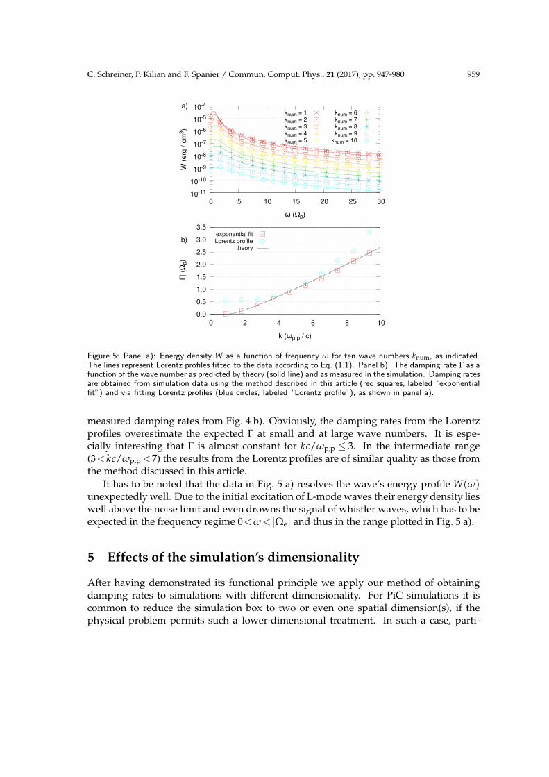
wave. We treat the amplitude W0 and the damping rate Γ as free parameters in the fit, butfix the wave’s frequency ω0 at its theoretical value. The Lorentz profiles resulting fromthese fits are shown in Fig. 5 a) together with the data from the simulations.
The damping rates obtained from the Lorentz profiles are plotted over the wave num-ber in Fig. 5 b), together with theoretical predictions from Eqs. (2.1) and (2.2) and the
C. Schreiner, P. Kilian and F. Spanier / Commun. Comput. Phys., 21 (2017), pp. 947-980 959
10-11
10-10
10-9
10-8
10-7
10-6
10-5
10-4
0 5 10 15 20 25 30
W (
erg
/ c
m3)
ω (Ωp)
knum = 1knum = 2knum = 3knum = 4knum = 5
knum = 6knum = 7knum = 8knum = 9
knum = 10
a)
0.0
0.5
1.0
1.5
2.0
2.5
3.0
3.5
0 2 4 6 8 10
|Γ| (Ω
p)
k (ωp,p / c)
exponential fitLorentz profile
theory
b)
Figure 5: Panel a): Energy density W as a function of frequency ω for ten wave numbers knum, as indicated.The lines represent Lorentz profiles fitted to the data according to Eq. (1.1). Panel b): The damping rate Γ as afunction of the wave number as predicted by theory (solid line) and as measured in the simulation. Damping ratesare obtained from simulation data using the method described in this article (red squares, labeled “exponentialfit”) and via fitting Lorentz profiles (blue circles, labeled “Lorentz profile”), as shown in panel a).
measured damping rates from Fig. 4 b). Obviously, the damping rates from the Lorentzprofiles overestimate the expected Γ at small and at large wave numbers. It is espe-cially interesting that Γ is almost constant for kc/ωp,p ≤ 3. In the intermediate range(3< kc/ωp,p <7) the results from the Lorentz profiles are of similar quality as those fromthe method discussed in this article.
It has to be noted that the data in Fig. 5 a) resolves the wave’s energy profile W(ω)unexpectedly well. Due to the initial excitation of L-mode waves their energy density lieswell above the noise limit and even drowns the signal of whistler waves, which has to beexpected in the frequency regime 0<ω< |Ωe| and thus in the range plotted in Fig. 5 a).
5 Effects of the simulation’s dimensionality
After having demonstrated its functional principle we apply our method of obtainingdamping rates to simulations with different dimensionality. For PiC simulations it iscommon to reduce the simulation box to two or even one spatial dimension(s), if thephysical problem permits such a lower-dimensional treatment. In such a case, parti-

960 C. Schreiner, P. Kilian and F. Spanier / Commun. Comput. Phys., 21 (2017), pp. 947-980
cle velocities and electromagnetic fields can still be treated as three-dimensional vectors.However, the particles may then only move along those directions which are still spa-tially resolved.
For the study of cyclotron damping of parallel propagating waves only one spatialdimension is essential, namely the direction parallel to the background magnetic fieldalong which the waves propagate. We therefore set up simulations using the physicaland numerical parameters given in Tables 1 and 2 in Section 3.1 in one-, two-, and three-dimensional simulation boxes. As in the example simulations discussed in Section 4 wecarry out sets of two simulations each, where waves with even knum are excited in onesimulation, and waves with odd knum in the other.
The specific initial conditions of a simulation are the result a random distributionof the particles and their velocities. Therefore, by chance, it may be that those randomconditions cause the simulation to yield atypical results, which is why one should inprinciple repeat each simulation with a different random particle distribution. To reducethe influence of the initial conditions on the final results of the simulations, we repeateach simulation six times, each time with a different seed for the random number gen-erator which produces the initial positions and velocities of the particles. That meansthat we perform six (random seeds) times two (even/odd wave numbers) times three(dimensionality) simulations.
To be able to refer to the individual simulations, we define the following nomencla-ture: Three-dimensional simulations will be referred to as set A, two-dimensional simu-lations as set B and one-dimensional simulations as set C. All simulations of a set whichinclude excited waves with odd (even) knum will be denoted by an index 1 (2), e.g. A1
(A2). Within a set, field data from all simulations of the same type (e.g. all simulations oftype A1) is averaged.
In Section 4.1 we have defined the interval tint (measured in time steps ∆t) whichdefines the number of time steps included in the dispersion plots (see Fig. 2) and the timeresolution for the energy density W(t) (see Fig. 3). To test the effect of tint we perform theanalysis of our simulations with three different interval lengths tint=1000∆t (=0.22Ω−1
p ),
tint=3000∆t (=0.67Ω−1p ), and tint =5000∆t (=1.12Ω−1
p ).
Starting with the three-dimensional simulations of set A, we present the results of ourstudy on the effect of the simulation’s dimensionality in the following sections.
5.1 Three-dimensional simulations
5.1.1 Particle statistics and temperature
In a setup which aims at transferring energy from the electromagnetic fields of plasmawaves to the particles, it is especially worthwhile to take a look at the particle populationand its velocity spectrum. Hence, before we start with analyzing the damping rates ofplasma waves, we take a look at the velocity distributions of protons and electrons. Atdifferent points in time during the simulation, the full particle data is stored for later

C. Schreiner, P. Kilian and F. Spanier / Commun. Comput. Phys., 21 (2017), pp. 947-980 961
0.95
1.00
1.05
1.10
1.15
1.20
1.25
0 2 4 6 8 10 12
T (
a.u
.)
t (1 / Ωp)
T⊥,p / T||,p
T⊥,p / T||,p
T⊥,e / T||,e
T⊥,e / T||,e
Tp / Te
Tp / Te
Tp / Tp(t=0)
Tp / Tp(t=0)
Figure 6: Proton and electron temperature characteristics throughout the simulations. All data is averaged oversimulations AI1 to AVI1 (bright colors, solid lines) or AI2 to AVI2 (darker colors, dashed lines), respectively.Indices ’p’ and ’e’ refer to protons and electrons, ’‖’ and ’⊥’ refer to components parallel and perpendicular tothe background magnetic field. See text for details.
examination. Studying the development of the velocity spectra of both electrons andprotons yields information about temperature changes and other kinetic effect duringthe simulation.
As stated before, we consider a thermal plasma, which means that the spectrum ofeach velocity component (in Cartesian coordinates vs,x, vs,y and vs,z, with ’s’ denoting theparticle species) follows a Gaussian distribution and the spectrum of the absolute of thevelocities (vs=|~vs|) follows a Maxwell-Boltzmann distribution. Protons and electrons canbe analyzed separately. Velocity data is binned, giving the particle number per bin as afunction of vs or a component of~vs, which then can be fitted by the respective distributionfunction. This procedure yields a temperature Ts, as well as temperatures T‖,s and T⊥,s
parallel and perpendicular to the background magnetic field ~B for each species. As forT‖,s and T⊥,s, the former is produced from the one velocity component parallel to ~B0,whereas the latter is the average over the two temperatures obtained from the spectra ofthe two velocity components perpendicular to ~B0.
Fig. 6 shows temperature development over time. In this plot, all temperatures areaverages over six simulations, where we have analyzed the data of simulations A1 andA2 separately. Errors are calculated from the standard errors of the temperatures derivedfrom the data of every single simulation.
The plot shows that at the beginning of the simulation an anisotropy in the protontemperature is evident, with T⊥,p being larger than T‖,p. This is a result of the initial-ization mechanism used for the excitation of waves: particles are initialized with a ther-mal spectrum, but are then pushed according to the electromagnetic fields of the excitedwaves. This leads to larger velocity components perpendicular to ~B0, while the parallelvelocity component is not affected. The effect increases for waves with frequencies closerto the resonance at Ωp, which is the reason for a more significant anisotropy in the data

962 C. Schreiner, P. Kilian and F. Spanier / Commun. Comput. Phys., 21 (2017), pp. 947-980
from A2 as compared to A1. Electrons are barely affected, though, as can be seen in Fig. 6.The additional energy given to the proton population during initialization also leads
to the proton temperature being higher than the electron temperature.In the course of the simulation, the anisotropy in proton temperature increases fur-
ther, which suggests that field energy from the decaying waves is transferred to the pro-tons. Again, electrons are not affected, as is expected for a proton cyclotron resonance.With the protons’ energy increasing, the temperature Tp also increases as compared tothe temperature at tΩp=0. The electron temperature stays constant throughout the sim-ulation and is therefore not shown in Fig. 6.
Note that the proton temperature and the anisotropy therein rises fastest at the be-ginning of the simulation (tΩp =0 to tΩp =6) and then remains relatively constant. Thissuggests that the energy transfer is faster at the beginning of the simulation and slowsdown later on, which is also expected from an exponential decay of the waves’ electro-magnetic fields.
Additional information is given in Appendix A, where we show velocity spectra fromone of the simulations of set A. These spectra illustrate the anisotropy of proton velocitiesat the beginning and at the end of the simulation and support the results presented in thissection.
5.1.2 Damping rates
We investigate the damping rates of the different waves with numerical wave numbersknum=1,2,3,4,5,6,7,8,9,10 in set A. As a reference, the theoretical damping rates are cal-culated from Eqs. (2.1) and (2.2), where two sets of parameters are used. While the plasmafrequency and the cyclotron frequencies of protons and electrons can be taken from Ta-ble 1 in Section 3.1, the temperature has to be corrected, as Section 5.1.1 has shown thatan anisotropy of the proton temperature is evident. Since the anisotropy is different insimulations A1 and A2, two values (T⊥,p/T‖,p)1=1.15 and (T⊥,p/T‖,p)2=1.20 are chosenaccording to the data in Fig. 6 at t=0. Similarly, the absolute temperature of the protonshas to be corrected to (Tp/Te)1 = 1.10 and (Tp/Te)2 = 1.13. The resulting damping ratesfrom Eqs. (2.1) and (2.2) are still not expected to describe simulation results perfectly,since the temperature changes throughout the simulation, as was shown in Fig. 6. Thetheoretical expectations are given in Table 7 in Appendix B.
To evaluate the simulation data, dispersion relations are created from the electromag-netic fields of all simulations of set A, as described in Section 4.1. The energy density ofeach excited wave is extracted from the dispersion plots for different points in time in thesimulations. The total energy density W(k) of a wave with wave number k is obtained bysumming up the components perpendicular to the background magnetic field ~B0 of boththe electric and magnetic fields. Afterwards a mean energy density W(k) is calculatedby averaging over the energy densities obtained from the individual simulations of setA. Note that set A has to be subdivided into A1 and A2 since waves with odd knum areexcited only in set A1 and waves with even knum are only present in set A2.
In a similar manner an average of the energy density Wnoise(k) of the background

C. Schreiner, P. Kilian and F. Spanier / Commun. Comput. Phys., 21 (2017), pp. 947-980 963
0.0
0.5
1.0
1.5
2.0
2.5
3.0
|Γ| (Ω
p)
tint = 1k Δttint = 3k Δttint = 5k Δt
theory (Tp / Te = 1.10)theory (Tp / Te = 1.13)
fit (tint = 1k Δt)fit (tint = 3k Δt)fit (tint = 5k Δt)
a)
-0.10
-0.05
0.00
0.05
0.10
0 2 4 6 8 10
ΔΓ /
Γ-
k (ωpp / c)
tint = 1k Δttint = 3k Δttint = 5k Δt
b)
Figure 7: Measured and theoretical damping rates Γ (panel a) and relative difference thereof (panel b) asfunctions of the parallel wave number k. Panel a): Fits to the simulation data are performed according toEq. (4.3); error bars represent standard errors. Panel b): ∆Γ/Γ is calculated according to Eq. (5.1); data atknum =0 is excluded due to the large deviation from theory (see text).
noise can be obtained. Since waves with even (odd) knum are not excited in simulationsA1 (A2), the background energy density at each relevant k can be extracted from the dis-persion relations as well. A corrected energy density of the excited waves is then obtainedsimply by subtracting Wnoise(k) from W(k). For the sake of less confusing notation, theenergy density will be denoted by W(k) throughout the article, although the correctedand averaged energy density is used when simulation data is presented.
Having obtained the energy density W(k) of each of the excited waves in the simula-tions of set A, the damping rates can be computed using the method described in Section4.2. These rates are also given in Table 7 in Appendix B. A plot representing the data ispresented in Fig. 7 a). Three different interval lengths tint have been used for data evalu-ation, meaning that we have used dispersion relations built from tint =1000,3000,5000time steps ∆t to extract the energy densities of the electromagnetic fields of the excitedwaves. Plots showing the energy densities W over time for all ten waves and the threeinterval lengths can be found in Appendix B.
Looking at the data given in Table 7 in Appendix B, it can be seen that the deviationbetween the theoretical predictions for the two temperature settings is of the order of

964 C. Schreiner, P. Kilian and F. Spanier / Commun. Comput. Phys., 21 (2017), pp. 947-980
less than one percent (except for knum =1). Furthermore, it becomes obvious that the er-rors of the measured damping rates are typically much smaller than the actual deviationof measured data and theoretical prediction. The errors given are computed from thestandard errors of the averaged electromagnetic fields obtained from the dispersion plotsvia Gaussian error propagation. However, this method seems not to capture the actualdeviation from theory. We therefore calculate the deviation
∆Γ/Γ=Γsim−Γtheory
0.5(
Γsim+Γtheory
) (5.1)
of measured and theoretical damping rate and present the results in Fig. 7 b). Note thatdifferent theoretical predictions are used for odd and even knum, as described above.
Both the curves in Fig. 7 a) and Fig. 7 b), showing the damping rate Γ and its deviationfrom theory as a function of the wave number k, suggest that our measurements are ingood agreement with theoretical prediction over a wide range of wave numbers. Judgingonly from observations with the naked eye, all measured damping rates in Fig. 7 are inperfect agreement with theory up to kc/ωpp ∼7 – a claim which is also supported bythe fits according to Eq. (4.3). At larger k the measured damping rates lie above thetheoretical predictions. Note that the fits are performed using all data, neglecting thedifferent temperature settings in simulations A1 and A2. Fit parameters are given inTable 3.
Table 3: Fit parameters including standard errors for the fits to the data of set A in Fig. 7 a) according toEq. (4.3).
tint(∆t) m1 m2 m3
1000 0.118±0.004 1.391±0.017 2.64±0.11
3000 0.119±0.008 1.38±0.03 2.6±0.3
5000 0.101±0.012 1.45±0.06 2.1±0.5
Taking a closer look at the relative deviations in Fig. 7 b), it can be confirmed thatthe simulations yield an accurate representation of cyclotron damping. In between ∼2<kc/ωpp <∼7 the deviation ∆Γ/Γ is mainly below two percent. This is especially inter-esting to notice, since the deviation between theoretical predictions for different protontemperatures is in the order just short of one percent. With the plasma being heatedduring the simulations – which makes theoretical predictions only an estimate – it canbe expected that measured data and theoretical prediction will differ at least by the sameamount as theoretical predictions for the temperatures at the beginning and the end of thesimulation. Keeping that in mind, a deviation below two percent appears to be perfectlyreasonable and accurate. The deviations of simulation data and theory for kc/ωpp < 2and kc/ωpp > 7 is around five percent, which still yields an appropriate estimate of thedamping rate in these regimes. Note that the data point at knum = 1 (kc/ωpp ∼ 0.9) isnot shown in Fig. 7 b). This case will be treated separately in Appendix C, since the

C. Schreiner, P. Kilian and F. Spanier / Commun. Comput. Phys., 21 (2017), pp. 947-980 965
time evolution of the energy density of the wave with knum=1 hints at unforeseen effectswhich hinder the measurement of the damping rate. For the following studies of one-and two-dimensional simulations in Sections 5.3 and 5.2 the wave with knum=1 will alsobe excluded.
The results presented in Fig. 7 suggest that the length of the interval tint do not influ-ence the overall results. The idea behind the different interval lengths is to trade temporalresolution (small tint) for more meaningful averages of the energy density over time (largetint), suppressing fluctuations on short time scales. However, the results are similar in allcases and thus no approach is preferred above the other two.
5.2 Two-dimensional simulations
In this section we present data obtained from set B, a set of twelve two-dimensionalsimulations analogous to set A (see Section 5.1). Independent of the dimensionality ofthe simulation, the method to determine the damping rates of excited waves is still thesame.
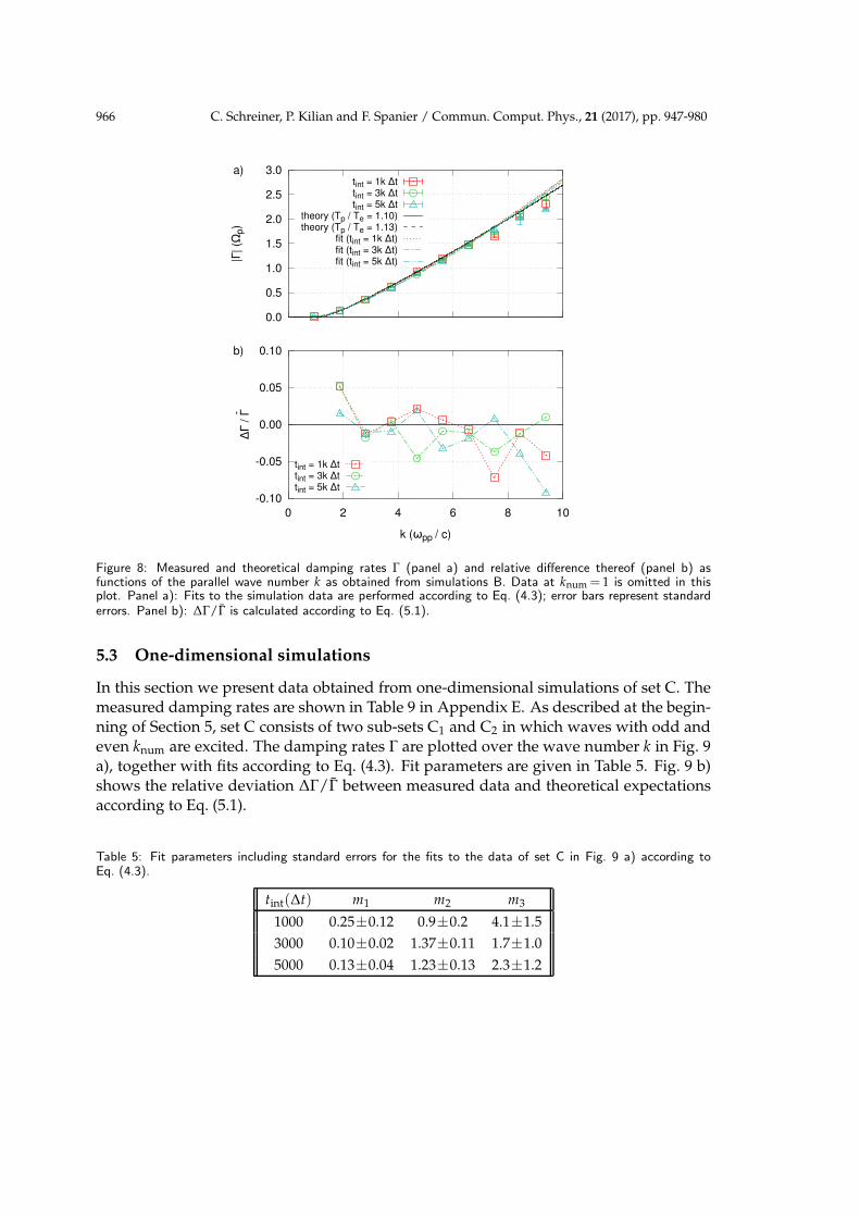
The obtained damping rates are shown in Table 8 in Appendix D. Like set A, set Bconsists of two sub-sets B1 and B2 in which waves with odd and even knum are excited.The damping rates Γ are plotted over the wave number k in Fig. 8 a), together with fitsaccording to Eq. (4.3). Fit parameters are given in Table 4. Fig. 8 b) shows the relativedeviation ∆Γ/Γ of measured data and theoretical expectations according to Eq. (5.1).
Table 4: Fit parameters including standard errors for the fits to the data of set B in Fig. 8 a) according toEq. (4.3).
tint(∆t) m1 m2 m3
1000 0.155±0.014 1.24±0.05 3.3±0.3
3000 0.125±0.009 1.33±0.03 2.7±0.3
5000 0.192±0.016 1.11±0.04 4.0±0.4
The measured data tend to underestimate the damping rates at high k, as Fig. 8 a)suggests. This is confirmed by Fig. 8 b), which shows a trend towards negative deviation∆Γ/Γ at kc/ωpp > 6. This trend is persistent for all three different interval lengths tint.However, in the range ∼2 < kc/ωpp <∼7 the relative deviation is again mainly belowtwo percent, indicating good agreement of simulation data and theoretical expectations.
The standard errors given in Table 8 in Appendix D approach the actual deviationfrom the theoretical predictions, as they are of the order of a few percent over the wholerange of wave numbers.
Measured energy densities W are plotted over time in Fig. 16 for tint =1000,3000,5000∆t. Here, the impact of the two-dimensional setup becomes obviousin the energy level of background noise Wnoise, which is about two orders of magnitudeabove the noise levels found in set A (see Fig. 14 in Appendix B). This leaves less spacefor the exponential fits (black lines) and thus potentially reduces the quality of the results.
966 C. Schreiner, P. Kilian and F. Spanier / Commun. Comput. Phys., 21 (2017), pp. 947-980
0.0
0.5
1.0
1.5
2.0
2.5
3.0
|Γ| (Ω
p)
tint = 1k Δttint = 3k Δttint = 5k Δt
theory (Tp / Te = 1.10)theory (Tp / Te = 1.13)
fit (tint = 1k Δt)fit (tint = 3k Δt)fit (tint = 5k Δt)
a)
-0.10
-0.05
0.00
0.05
0.10
0 2 4 6 8 10
ΔΓ /
Γ-
k (ωpp / c)
tint = 1k Δttint = 3k Δttint = 5k Δt
b)
Figure 8: Measured and theoretical damping rates Γ (panel a) and relative difference thereof (panel b) asfunctions of the parallel wave number k as obtained from simulations B. Data at knum = 1 is omitted in thisplot. Panel a): Fits to the simulation data are performed according to Eq. (4.3); error bars represent standarderrors. Panel b): ∆Γ/Γ is calculated according to Eq. (5.1).
5.3 One-dimensional simulations
In this section we present data obtained from one-dimensional simulations of set C. Themeasured damping rates are shown in Table 9 in Appendix E. As described at the begin-ning of Section 5, set C consists of two sub-sets C1 and C2 in which waves with odd andeven knum are excited. The damping rates Γ are plotted over the wave number k in Fig. 9a), together with fits according to Eq. (4.3). Fit parameters are given in Table 5. Fig. 9 b)shows the relative deviation ∆Γ/Γ between measured data and theoretical expectationsaccording to Eq. (5.1).
Table 5: Fit parameters including standard errors for the fits to the data of set C in Fig. 9 a) according toEq. (4.3).
tint(∆t) m1 m2 m3
1000 0.25±0.12 0.9±0.2 4.1±1.5
3000 0.10±0.02 1.37±0.11 1.7±1.0
5000 0.13±0.04 1.23±0.13 2.3±1.2

C. Schreiner, P. Kilian and F. Spanier / Commun. Comput. Phys., 21 (2017), pp. 947-980 967
0.0
0.5
1.0
1.5
2.0
2.5
3.0
|Γ| (Ω
p)
tint = 1k Δttint = 3k Δttint = 5k Δt
theory (Tp / Te = 1.10)theory (Tp / Te = 1.13)
fit (tint = 1k Δt)fit (tint = 3k Δt)fit (tint = 5k Δt)
-0.4
-0.3
-0.2
-0.1
0.0
0.1
0 2 4 6 8 10
ΔΓ /
Γ-
k (ωpp / c)
tint = 1k Δttint = 3k Δttint = 5k Δt
Figure 9: Measured and theoretical damping rates Γ (panel a) and relative difference thereof (panel b) asfunctions of the parallel wave number k as obtained from simulations C. Data at knum = 1 is omitted in thisplot. Panel a): Fits to the simulation data are obtained according to Eq. (4.3); error bars represent standarderrors. Panel b): ∆Γ/Γ is calculated according to Eq. (5.1).
The measured data tend to underestimate the damping rates even more than in thecase of the two-dimensional setup presented in Section 5.2. Fig. 9 a) shows that the mea-sured data deviate from the theoretical expectations already at kc/ωpp>4 in a systematicmanner. This behavior becomes even more evident when looking at the fits to the dataor at the relative deviation plotted in Fig. 9 b).
Contrary to the results from the three- and two-dimensional simulations (see Sections5.1 and 5.2), the data in Fig. 9 b) do not exhibit a region in k where the relative deviationis at a relatively constant and low level. Starting already at smallest k a steady downwardtrend can be observed, leading to deviations of up to ∼40 percent.
The standard errors given in Table 9 in Appendix E are in the order of a few to morethan ten percent over the whole range of wave numbers. However, in many cases thisrather large uncertainty does not cover the theoretical predictions. Note that the fits tothe data also become more and more unreliable, as the errors in Table 5 show. Especiallyparameter m3, which is part of the argument of the exponential function in Eq. (4.3),shows standard errors of up to ∼60 percent.
Measured energy densities W are plotted over time in Fig. 17 in Appendix E for tint=

968 C. Schreiner, P. Kilian and F. Spanier / Commun. Comput. Phys., 21 (2017), pp. 947-980
1000,3000,5000∆t. Here, the impact of the one-dimensional setup becomes obviousin the energy level of background noise Wnoise, which is about four orders of magnitudeabove the noise levels found in set A (see Fig. 14 in Appendix B). The energy range inwhich the exponential fits can be applied is thus narrowed down to one to two ordersof magnitude in W, which reduces the quality of the fits drastically. It can be expectedthat the correct slope of the exponential function is not represented in the data, since theregion between the slow onset of wave damping and the background noise level is notsufficiently broad.
6 Comparison of simulations with different parameter sets
In this section, the physical parameters given in Table 1 in Section 3.1 are varied, whereasmost of the numerical parameters from Table 2 are kept constant. The resulting set ofsimulations, set D, consists of six individual simulations (D1 through D6), each containingfive excited waves. The change of the background magnetic field B0, the thermal speedvth, and the plasma frequency ωp leads to a change in the plasma beta (e.g. [10])
β=8πnkB T/B20, (6.1)
where n = ne+np is the particle number density (electrons and protons) and kB is theBoltzmann constant. Assuming that the plasma temperature is the same for electronsand protons, Te=Tp =T, and that ne=np, the above equation can be written as
β=4ω2
p,ev2th,e
Ω2e c2
. (6.2)
We will use this definition of β to better describe and refer to the individual simulationsof set D. A list of parameters used for each of the six simulations is presented in Table 6.Parameters not listed, such as N‖, N⊥ and mp/me are the same as in Table 2 in Section3.1. The number of time steps has been set to Nt =50000 in all simulations except for D3,where Nt=100000.
Table 6: Physical and numerical parameters for the simulations of series D.
simulation ωp,e(rads−1) |Ωe|(ωp,e) vth,e(c) β ∆x(cω−1p,e) ∆t(ω−1
p,e)
D1 2.0·108 2.64·10−1 0.05 0.144 3.53·10−2 2.04·10−2
D2 2.0·108 8.79·10−1 0.05 0.013 3.53·10−2 2.04·10−2
D3 2.0·108 4.40·10−1 0.02 0.008 1.41·10−2 8.16·10−3
D4 2.0·108 4.40·10−1 0.10 0.207 7.04·10−2 4.06·10−2
D5 5.0·107 1.76 0.05 0.003 3.53·10−2 2.04·10−2
D6 5.0·108 1.76·10−1 0.05 0.323 3.53·10−2 2.04·10−2

C. Schreiner, P. Kilian and F. Spanier / Commun. Comput. Phys., 21 (2017), pp. 947-980 969
0
1
2
3
4
5
6
|Γ| (Ω
p)
D1D2D3D4D5D6A
theory (D1)theory (D2)theory (D3)theory (D4)theory (D5)theory (D6)theory (A)
a)
-0.4
-0.2
0.0
0.2
0.4
0 2 4 6 8 10 12
ΔΓ /
Γ-
k (ωpp / c)
D1 ( = 0.144)D2 ( = 0.013)D3 ( = 0.008)D4 ( = 0.207)D5 ( = 0.003)D6 ( = 0.323)
b)
Figure 10: Panel a): Measured damping rates Γ from simulations with different physical setups (sets A andD, see text for details). Theoretical curves are given for comparison. Panel b): Relative deviation of measureddata and theoretical predictions for set D. The first point of data for simulation D5 lies at ∆Γ/Γ=1.63, but iscut off in this plot.
The measured damping rates for the six simulations of set D are shown together withthose obtained from the data of set A in Fig. 10. An interval length tint=1000∆t has beenused. Lines represent theoretical predictions from Eqs. (2.1) and (2.2), where Te =Tp =Tis assumed. Fits to the data are omitted here.
Because of the different sets of physical parameters and the resulting β in each of thesimulations, the dispersion curves and especially the shape of Γ(k) also change, as canbe seen in Fig. 10 a). The plot reveals two trends: First, above |Γ|/Ωp ≃ 3 the deviationof measured data and theoretical model increases. This is due to the fast damping of thewave, which makes reliable measurements hard to obtain. Secondly, the measurementssuggest that the simulations underestimate the damping rates at low β, as can be seenwhen looking at D2, D3 and D5. The reason for this second trend is unclear to us, but willbe examined in more detail in the following paragraphs.
Fig. 10 b) depicts the relative deviation of measured data and theory, with the devia-tion ∆Γ/Γ being defined by Eq. (5.1). This plot makes the disagreement of measurementand theoretical model in the case of low β plasmas even more clear. With the exceptionof the first point of data, the curves for D2, D3 and D5 suggest an underestimation of the

970 C. Schreiner, P. Kilian and F. Spanier / Commun. Comput. Phys., 21 (2017), pp. 947-980
10-13
10-12
10-11
10-10
10-9
10-8
10-7
10-6
10-5
10-4
0 5 10 15 20 25 30 35 40 45
W (
erg
/ c
m3)
t (1 / Ωp)
knum = 1knum = 2knum = 3knum = 4knum = 5
a)
0
0.1
0.2
0.3
0.4
0.5
0 2 4 6 8 10
|Γ| (Ω
p)
k (ωpp / c)
D5 (early)D5 (late)
theory (D5)
b)
Figure 11: Panel a): Energy density W of the excited waves in simulation D5 as a function of time. For mostwaves two intervals can be found in which an exponential fit can be applied to the data (“early” and “late”),as shown by the solid and dotted black lines. Panel b): Measured damping rates as a function of the wavenumber k, together with theoretical predictions.
damping rate by 20 to 40 percent. The first data point for D3 and D5 suggests that at verylow damping rates, the measurement is not reliable and significantly overestimates theactual damping rate, as discussed at the end of Section 5.1.2 and in Appendix C. The sim-ulations with higher β exhibit deviations of less than ten percent over the whole range ofwave numbers.
In the case of simulations with a low β, wave damping is underestimated, as can beseen in Figs. 10 a) and b). However, the damping rates presented above have been ob-tained with a very benevolent choice of original data for the exponential fits to the energydensity W. In fact, in some cases it would be possible to find a different exponential fit toW later in the simulations, as depicted for simulation D5 in the top panel of Fig. 11. Here,the exponential fits used above are shown as solid black lines, whereas alternative fits arerepresented by dotted black lines. As can be seen, the energy density exhibits the usualtransit to an exponential decay at the beginning of the simulation, as discussed in Section4. At later times in the simulation, the exponential decay slows down and eventuallytransitions into a region with a different slope which can be interpreted as exponentialdecay with a different damping rate.
Panel b) of Fig. 11 shows the measured damping rates together with theoretical pre-

C. Schreiner, P. Kilian and F. Spanier / Commun. Comput. Phys., 21 (2017), pp. 947-980 971
dictions. The terms “early” and “late” refer to the intervals in simulation time, in whichthe damping rates have been determined, i.e. the solid and dotted lines in the top panelof Fig. 11. It can be easily seen that the agreement of measurement and model is evenworse when the “late” damping rates are considered. Unfortunately, the reason for thebehavior of the waves’ energy densities throughout the simulation are unknown to us.
7 Discussion and conclusions
In this article we have suggested a simple test setup for simulating cyclotron dampingusing a PiC approach and presented a method to obtain the damping rate of a given wavefrom simulation data, equivalent to the method of Koen et al. [1]. As long as electromag-netic field data is produced and saved to disk several times during the simulation, themethod described in Section 4 can be used to derive the damping rate of a wave fromdispersion plots produced from the field data at different points in time. If Fourier trans-formed (k-space) field data is available at run-time, it is even sufficient to write only thefield data (or energy) at specific wave numbers k, that are of interest for later analysis,to disk and thus reduce the required output dramatically. Our method is not necessarilylimited to PiC simulations, but can in principle be used with any numerical approachto plasma physics – as long as the approach used supports the interactions leading tocyclotron damping, of course.
Using our mechanism for wave excitation (see Section 3.1 or [3]) we set up two ex-ample simulations which are then evaluated in Section 4 in order to give some practicalinsight into the analysis needed to obtain damping rates. Our analysis shows that theexcitation of several left-handed, circularly polarized, low frequency waves (in the fre-quency range between Alfven and ion cyclotron waves) leads to cyclotron damping bythermal protons, as expected. Cyclotron damping leads to a transfer of energy from theelectromagnetic fields of the damped waves to the resonant particles. Thus, a characteris-tic decline of the energy density W of the wave can be found. With the method describedin Section 4, we are able to reproduce the energy density W(t) of each excited wave as afunction of time. The application of an exponential fit to W(t) then yields the dampingrate Γ.
Repeating this procedure for several waves at different wave numbers k‖ yields anestimate for Γ(k‖), which can be compared to theoretical predictions from warm plasmatheory. Results from our example simulations exhibit an acceptable overall agreementwith theory, as Fig. 4 b) in Section 4.2 shows. This result is particularly interesting, sincethe excited waves on the low frequency branch of the L-mode are not resolved in thedispersion plots. Finding the correct damping rate can therefore be seen as a proof forthe correct behavior of these waves in the simulation.
For comparison, we determine the damping rates of the same waves again, usinga different method. Using Lorentz profiles to describe the spectral energy distributionW(ω) of a wave yields the damping rate, which is the half width at half maximum of the

972 C. Schreiner, P. Kilian and F. Spanier / Commun. Comput. Phys., 21 (2017), pp. 947-980
distribution. The results obtained in Section 4.3 suggest that this method is less reliablethan the new method characterized in this article.
Better results from the Lorentz profiles are expected if a higher spectral resolution ofthe waves in question is available and both flanks of the distribution can be seen. How-ever, for the case of damped L-mode waves at low frequencies, such a high spectral reso-lution cannot be achieved, since resolution increases with the run time of the simulation.Run time cannot be increased indefinitely, as the waves will be dissipated completelyafter a finite amount of time.
The method of Koen et al. [1] does not suffer from low spectral resolution, as shownin Section 4.2. As has been demonstrated in our example, damping rates can even beobtained if the frequency of the respective wave is not resolved at all. This is, of course,limited to the case in which only one wave mode is under-resolved. As soon as the spec-tral resolution of the dispersion plots is so low that several wave modes are mapped intothe same (or the lowest) frequency bin, the wave modes can no longer be distinguishedand our method to determine damping rates breaks down.
Of course, our method can also be applied to right-handed waves on the whistlerbranch or electron cyclotron waves. In this case, it should be possible to extract the fre-quency and the damping rate and thus compare both to the theoretical dispersion rela-tion. So far, we have only studied purely parallel propagating waves. However, it shouldalso be possible to use the method described in Section 4 to determine damping rates ofoblique waves, although obtaining accurate theoretical predictions might be more com-plicated in this case.
In Section 5 we wave tested the influence of the simulation’s spatial dimensions on therepresentation of waves and cyclotron damping. Since PiC simulations require relativelylarge amounts of computing time, it is often attempted to reduce the computational costby reducing the spatial dimensions in the simulation. In theory, this can also be donein the case of cyclotron damping of parallel propagating waves, since only the directionparallel to the background magnetic field B0 has to be resolved. Thus, two- or evenone-dimensional simulations are possible, as long as electromagnetic fields and particlevelocities are still treated as three-dimensional vectors.
The comparison of results from three- (Section 5.1), two- (Section 5.2) and one-dimensional (Section 5.3) simulations shows that the accuracy of the measurement of thedamping rate decreases drastically when the dimensionality of the simulation is reduced.The key problem is the reduced number of particles in simulations with less spatial di-mensions, which leads to an increase in background noise and thus to a reduced signalto noise ratio.
We have kept the number of particles per cell constant while decreasing the number ofcells in the simulation, thus reducing the total particle count. One could also increase thenumber of particles per cell to maintain the total number of particles, i.e. perform a one-or two-dimensional simulation with the same number of particles as a correspondingthree-dimensional simulation. In this latter case we expect better results from two- orone-dimensional simulations. However, such simulations are often not feasible, since
C. Schreiner, P. Kilian and F. Spanier / Commun. Comput. Phys., 21 (2017), pp. 947-980 973
the computational effort – to first order – scales with the total number of particles persimulation. Thus, the advantage of a two-dimensional simulation vanishes, if the particlecount is as high as it would be in three dimensions.
Lastly, in Section 6 we present results from three-dimensional simulations with differ-ent sets of physical parameters. We find that our simulations reproduce the expected cy-clotron damping with reasonable deviation from theory only in a certain range of plasmabetas. As Fig. 10 shows, the deviations from theory increase for small plasma betas.
Overall, we argue that PiC simulations are capable of reproducing cyclotron damp-ing correctly. However, not every physical or numerical configuration might be suitablefor this endeavor. The article at hand concentrates more on the general method of de-termining the damping rate from a set of simulation data and compares results of a fewdifferent simulations. However, it might also be worthwhile to investigate wave damp-ing with different numerical schemes, such as hybrid PiC/MHD codes or Vlasov codes,and compare these numerical approaches.
Acknowledgments
The authors gratefully acknowledge the Gauss Centre for Supercomputing e.V.(www.gauss-centre.eu) for funding this project by providing computing time on the GCSSupercomputer SuperMUC at Leibniz Supercomputing Centre (LRZ, www.lrz.de).
This work is based upon research supported by the National Research Foundationand Department of Science and Technology. Any opinion, findings and conclusions orrecommendations expressed in this material are those of the authors and therefore theNRF and DST do not accept any liability in regard thereto.
We acknowledge the use of the ACRONYM code and would like to thank the devel-opers (Verein zur Forderung kinetischer Plasmasimulationen e.V.) for their support.
The authors would like to thank Andreas Kempf for providing computational re-sources for some of the early test simulations and for many helpful comments on andoptimization of the piece of code which computes the warm plasma dispersion relations.
Appendix
A Velocity spectra
Fig. 12 shows the protons’ parallel and perpendicular velocity distributions at the startand at the end of one of the simulations of set A1. The spectra are shown in the toppanels (a and b) and the differences between the actual data and a Gaussian fit to thedata are presented in the bottom panels (c and d). Fig. 12 c) depicts the influence of theinitial particle boost on the velocity spectra: while the deviations from a pure Gaussianare random in v‖,p, the deviations in v⊥,p are systematic and symmetric around v⊥,p =0.

974 C. Schreiner, P. Kilian and F. Spanier / Commun. Comput. Phys., 21 (2017), pp. 947-980
0.0
0.2
0.4
0.6
0.8
1.0
1.2
pro
ton c
ount (a
.u.)
a)v||(t Ωp=0)
v⊥(t Ωp=0)
-0.001
0.000
0.001
-0.03 -0.02 -0.01 0.00 0.01 0.02 0.03
pro
ton c
ount (a
.u.)
v||,⊥ (c)
c)diff v||(t Ωp=0)
diff v⊥(t Ωp=0)
0.0
0.2
0.4
0.6
0.8
1.0
1.2b)v||(t Ωp=11.2)
v⊥(t Ωp=11.2)
-0.003
-0.002
-0.001
0.000
0.001
0.002
0.003
-0.03 -0.02 -0.01 0.00 0.01 0.02 0.03
v||,⊥ (c)
d)diff v||(t Ωp=11.2)
diff v⊥(t Ωp=11.2)
Figure 12: Distribution of the protons’ parallel and perpendicular velocity components at the start (panel a)and at the end (panel b) of a simulation and deviations from a pure Gaussian distribution (panels c and d,respectively). Particle numbers are normalized to the number of particles in the bin around v‖=0 at the start
of the simulation.
Excess particles can be found both at high and very low perpendicular speeds, whereasfewer particles can be found in the intermediate range.
At the end of the simulation, the perturbations in v⊥,p have not changed in shape,but the perturbations in v‖,p have (Fig. 12 d). Again, more particles can be found athigh and very low speeds, and fewer particles are present in the intermediate range.But unlike the deviations in v⊥,p, those in v‖,p are not symmetric. Deviations from the
Gaussian distribution are stronger in the direction parallel to ~B and less pronounced inthe direction anti-parallel to ~B.
Similar figures showing the distribution of velocity components of the electrons aredepicted in Fig. 13. Again, we show the distributions of parallel and perpendicular ve-locity components of the electrons at the start and at the end of a simulation panels a) andb). Panels c) and d) show the deviations of the actual data from Gaussian distributions.These plots prove that the electrons’ velocity spectra hardly diverge from a thermal dis-tribution at the start of the simulation (panels a and c). At the end of the simulation thespectrum of v‖,e deviates from a Gaussian distribution similarly to v‖,p, but with a lessprominent asymmetry (panel d).
We expect to find net momentum when summing up the momenta of all particles inthe simulations. Unfortunately, our analysis has shown that numerical fluctuations seemto dominate the total momentum of the particles, so that an effect of the decaying waveson the momentum of the whole particle population cannot be verified.

C. Schreiner, P. Kilian and F. Spanier / Commun. Comput. Phys., 21 (2017), pp. 947-980 975
0.0
0.2
0.4
0.6
0.8
1.0
1.2
ele
ctr
on c
ount (a
.u.)
a)v||(t Ωp=0)
v⊥(t Ωp=0)
-0.001
0.000
0.001
-0.15 -0.10 -0.05 0.00 0.05 0.10 0.15
ele
ctr
on c
ount (a
.u.)
v||,⊥ (c)
c)diff v||(t Ωp=0)
diff v⊥(t Ωp=0)
0.0
0.2
0.4
0.6
0.8
1.0
1.2b)v||(t Ωp=11.2)
v⊥(t Ωp=11.2)
-0.001
0.000
0.001
-0.15 -0.10 -0.05 0.00 0.05 0.10 0.15
v||,⊥ (c)
d)diff v||(t Ωp=11.2)
diff v⊥(t Ωp=11.2)
Figure 13: Distribution of the electrons’ parallel and perpendicular velocity components at the start (panel a)and at the end (panel b) of a simulation and deviations from a pure Gaussian distribution (panels c and d).Particle numbers are normalized to the number of particles in the bin around v‖=0 at the start of the simulation.
B Energy densities and damping rates obtained from set A
Table 7 contains the theoretical damping rates according to Eqs. (2.1) and (2.2), as ob-tained with the parameters given in Table 1 and the temperatures discussed in Section5.1.1. The measured damping rates from set A (three-dimensional simulations) is alsoincluded. Note that damping rates for waves with odd (even) knum have to be comparedto the theoretical values for Tp/Te =1.10 (1.13).
The average energy densities W (see Section 5.1.2 for details) of ten different waves insimulations A1 (odd knum) and A2 (even knum) are plotted over time in Fig. 14. The threepanels represent the data obtained from the simulations using the method described inSection 4 using intervals of length tint =1000,3000,5000∆t, with ∆t being the length ofone time step. While shorter tint yield higher temporal resolution (and more data pointsfor the fit to be applied to), a more representative average of the waves’ energies can beobtained during longer intervals, thus averaging out short time fluctuations. However,the overall behavior is the same for all tint: Damping starts slowly (no exponential decayof energy), then develops the characteristic exponential slope representing the dampingrate of each wave and finally cuts off when the energy of the wave is of the order of thebackground noise.
The background noise level Wnoise seems to depend on the interval length, sinceWnoise∼10−11erg/cm3 for tint=1000∆t and Wnoise∼10−12erg/cm3 for tint=3000,5000∆t.Note that energy densities below 10−13erg/cm3 are cut off, which is why there seem to

976 C. Schreiner, P. Kilian and F. Spanier / Commun. Comput. Phys., 21 (2017), pp. 947-980
Table 7: Theoretical and measured damping rates for ten different waves. Theoretical rates are given for twotemperature settings, matching the setups used in simulations A1 and A2 to obtain the damping rates at oddand even numbered knum, respectively.
knum |Γ|(Ωp)
theory: theory: simulation: simulation: simulation:
Tp/Te=1.10 Tp/Te=1.13 tint=1000∆t tint=3000∆t tint=5000∆t
T⊥,p/T‖,p=1.15 T⊥,p/T‖,p=1.20
1 3.599·10−4 3.548·10−4 (1.5502±0.0018)·10−2 (1.555±0.003) ·10−2 (1.549±0.002) ·10−2
2 0.1277 0.1268 0.13414±0.00004 0.13383±0.00006 0.13446±0.00007
3 0.3617 0.3586 0.35413±0.00011 0.35392±0.00017 0.3561±0.0003
4 0.6234 0.6180 0.6183±0.0004 0.6224±0.0007 0.6131±0.0005
5 0.9002 0.8926 0.8989±0.0010 0.8958±0.0013 0.9017±0.0018
6 1.189 1.179 1.1930±0.0016 1.1744±0.0009 1.1464±0.0008
7 1.486 1.475 1.523±0.004 1.519±0.003 1.4960±0.0017
8 1.792 1.779 1.878±0.008 1.885±0.005 1.863±0.004
9 2.105 2.091 2.218±0.015 2.146±0.003 2.202±0.012
10 2.425 2.409 2.524±0.017 2.548±0.007 2.53±0.04
10-13
10-12
10-11
10-10
10-9
10-8
10-7
10-6
10-5
10-4
0 2 4 6 8 10
W (
erg
/ c
m3)
t (1 / Ωp)
knum = 1knum = 2knum = 3knum = 4knum = 5knum = 6knum = 7knum = 8knum = 9
knum = 10
a)
0 2 4 6 8 10
t (1 / Ωp)
knum = 1knum = 2knum = 3knum = 4knum = 5knum = 6knum = 7knum = 8knum = 9
knum = 10
b)
0 2 4 6 8 10
t (1 / Ωp)
knum = 1knum = 2knum = 3knum = 4knum = 5knum = 6knum = 7knum = 8knum = 9
knum = 10
c)
Figure 14: Energy density of ten waves obtained in intervals of tint=1000∆t (panel a), tint=3000∆t (panel b)and tint = 5000∆t (panel c) from the data of simulations of set A. Black lines indicate exponential fits to thedata which yield the damping rates for the different waves.
be gaps in some data sets. The measured energy density curves appear to deviate fromthe expected exponential decay already above the noise limit. Most of the exponentialfits have therefore been cut off at higher energy densities (see black lines in Fig. 14). Areason for the unexpected deviation from the exponential decay could be the changingplasma temperature later on in the simulation.
C Weakly damped wave
One peculiarity in the data shown in Table 7 in Appendix B is the measured damping ratefor knum=1, which is almost two orders of magnitude above the theoretical expectations.

C. Schreiner, P. Kilian and F. Spanier / Commun. Comput. Phys., 21 (2017), pp. 947-980 977
1.0x10⁻⁵
1.1x10⁻⁵
1.2x10⁻⁵
1.3x10⁻⁵
0 5 10 15 20 25W
(erg
/ c
m3)
t (1 / Ωp)
1
2
knum=1
Figure 15: Energy density W of an excited wave with knum=1 in a rerun of a simulation of type A1. The grayline marks the end of the regular simulation, the black line labeled with ’1’ represents the exponential fit whichyields Γ(knum = 1) for tint = 1000∆t in Table 7 in Appendix B. The rerun simulation contains twice as manytime steps as the original run. Thus, an additional exponential fit can be obtained at later times, as indicatedby the black line labeled with ’2’. Note that the y-axis is in logarithmic scale.
We therefore examine the behavior of the wave with knum =1 more closely in a rerun ofone simulation of set A1. The energy density W is plotted over time t in Fig. 15, wheretint =1000∆t is used. The rerun uses the same physical and numerical parameters as theoriginal simulation (see Tables 1 and 2 in Section 3.1), but employs twice as many timesteps, thus doubling the physical time simulated.
The end of the regular simulation of type A1 is indicated by a gray line in Fig. 15.At the start of the simulation the energy density decreases exponentially, but seems tolevel out towards the end of the regular simulation time, with the energy density stillbeing way above the noise limit (Wnoise ≈10−11erg/cm3). The fit which lead to Γ(knum =1) for tint = 1000∆t in Table 7 in Appendix B is shown as a black line labeled with ’1’.In the second half of the simulation the energy density stays at a rather constant level,fluctuating only slightly. Applying another exponential fit to this regime (labeled with’2’ in Fig. 15) yields a different damping rate: Γrerun(knum =1)·Ωp =−(3±5)·10−5. Sinceonly one simulation has been carried out, no standard error can be calculated and onlythe statistical error from the fit is given.
Although the newly obtained damping rate is closer to the theoretical expectations,it is not very reliable due to the large error. Additionally, the runtime of the simulationhas to be twice as long as originally planned, thus doubling the computational effort ofthe simulation. The reason for the first exponential decay of the wave, visible betweentΩp =2 and tΩp =6 in Fig. 15, is unclear. However, no further investigations have beencarried out, since the regime of very weak damping (|Γ|≪Ωp) is not in the focus of thisstudy.
D Energy densities and damping rates obtained from set B
Table 8 contains theoretical and measured damping rates for the two-dimensional simula-tions of set B. Again, we give the theoretical values for two different proton temperatures
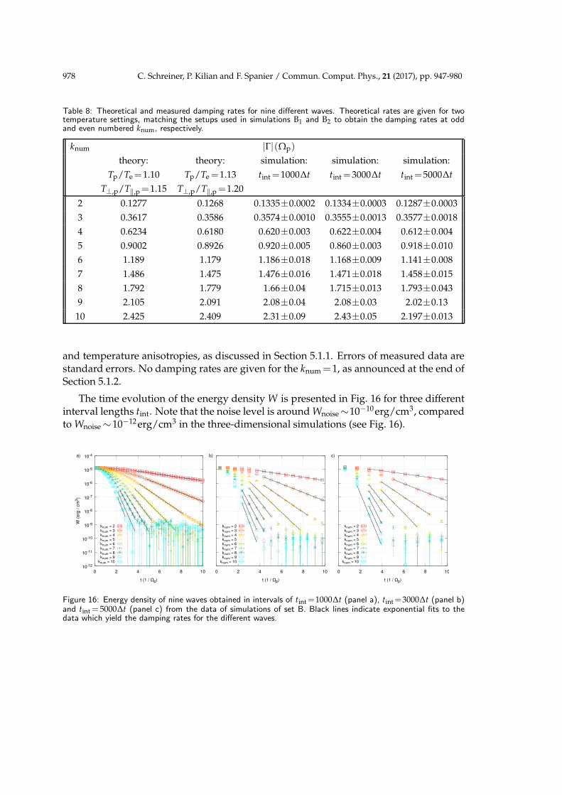
978 C. Schreiner, P. Kilian and F. Spanier / Commun. Comput. Phys., 21 (2017), pp. 947-980
Table 8: Theoretical and measured damping rates for nine different waves. Theoretical rates are given for twotemperature settings, matching the setups used in simulations B1 and B2 to obtain the damping rates at oddand even numbered knum, respectively.
knum |Γ|(Ωp)
theory: theory: simulation: simulation: simulation:
Tp/Te=1.10 Tp/Te=1.13 tint=1000∆t tint=3000∆t tint=5000∆t
T⊥,p/T‖,p=1.15 T⊥,p/T‖,p=1.20
2 0.1277 0.1268 0.1335±0.0002 0.1334±0.0003 0.1287±0.0003
3 0.3617 0.3586 0.3574±0.0010 0.3555±0.0013 0.3577±0.0018
4 0.6234 0.6180 0.620±0.003 0.622±0.004 0.612±0.004
5 0.9002 0.8926 0.920±0.005 0.860±0.003 0.918±0.010
6 1.189 1.179 1.186±0.018 1.168±0.009 1.141±0.008
7 1.486 1.475 1.476±0.016 1.471±0.018 1.458±0.015
8 1.792 1.779 1.66±0.04 1.715±0.013 1.793±0.043
9 2.105 2.091 2.08±0.04 2.08±0.03 2.02±0.13
10 2.425 2.409 2.31±0.09 2.43±0.05 2.197±0.013
and temperature anisotropies, as discussed in Section 5.1.1. Errors of measured data arestandard errors. No damping rates are given for the knum=1, as announced at the end ofSection 5.1.2.
The time evolution of the energy density W is presented in Fig. 16 for three differentinterval lengths tint. Note that the noise level is around Wnoise∼10−10erg/cm3, comparedto Wnoise ∼10−12erg/cm3 in the three-dimensional simulations (see Fig. 16).
10-12
10-11
10-10
10-9
10-8
10-7
10-6
10-5
10-4
0 2 4 6 8 10
W (
erg
/ c
m3)
t (1 / Ωp)
knum = 2knum = 3knum = 4knum = 5knum = 6knum = 7knum = 8knum = 9
knum = 10
a)
0 2 4 6 8 10
t (1 / Ωp)
knum = 2knum = 3knum = 4knum = 5knum = 6knum = 7knum = 8knum = 9
knum = 10
b)
0 2 4 6 8 10
t (1 / Ωp)
knum = 2knum = 3knum = 4knum = 5knum = 6knum = 7knum = 8knum = 9
knum = 10
c)
Figure 16: Energy density of nine waves obtained in intervals of tint=1000∆t (panel a), tint=3000∆t (panel b)and tint = 5000∆t (panel c) from the data of simulations of set B. Black lines indicate exponential fits to thedata which yield the damping rates for the different waves.
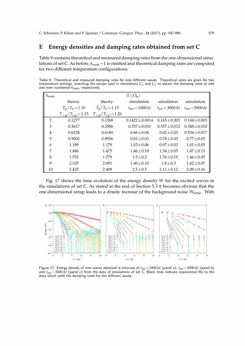
C. Schreiner, P. Kilian and F. Spanier / Commun. Comput. Phys., 21 (2017), pp. 947-980 979
E Energy densities and damping rates obtained from set C
Table 9 contains theoretical and measured damping rates from the one-dimensional simu-lations of set C. As before, knum=1 is omitted and theoretical damping rates are computedfor two different temperature configurations.
Table 9: Theoretical and measured damping rates for nine different waves. Theoretical rates are given for twotemperature settings, matching the setups used in simulations C1 and C2 to obtain the damping rates at oddand even numbered knum, respectively.
knum |Γ|(Ωp)
theory: theory: simulation: simulation: simulation:
Tp/Te =1.10 Tp/Te =1.13 tint=1000∆t tint=3000∆t tint=5000∆t
T⊥,p/T‖,p=1.15 T⊥,p/T‖,p=1.20
2 0.1277 0.1268 0.1422±0.0014 0.143±0.003 0.144±0.003
3 0.3617 0.3586 0.357±0.010 0.357±0.012 0.348±0.010
4 0.6234 0.6180 0.66±0.04 0.62±0.03 0.534±0.017
5 0.9002 0.8926 0.81±0.03 0.78±0.03 0.77±0.03
6 1.189 1.179 1.03±0.06 0.97±0.03 1.01±0.05
7 1.486 1.475 1.46±0.10 1.34±0.05 1.47±0.15
8 1.792 1.779 1.5±0.2 1.76±0.19 1.46±0.05
9 2.105 2.091 1.40±0.10 1.8±0.3 1.62±0.07
10 2.425 2.409 2.5±0.5 2.11±0.12 2.09±0.16
Fig. 17 shows the time evolution of the energy density W for the excited waves inthe simulations of set C. As stated at the end of Section 5.3 it becomes obvious that theone-dimensional setup leads to a drastic increase of the background noise Wnoise. With
10-10
10-9
10-8
10-7
10-6
10-5
10-4
0 2 4 6 8 10
W (
erg
/ c
m3)
t (1 / Ωp)
knum = 2knum = 3knum = 4knum = 5knum = 6knum = 7knum = 8knum = 9
knum = 10
a)
0 2 4 6 8 10
t (1 / Ωp)
knum = 2knum = 3knum = 4knum = 5knum = 6knum = 7knum = 8knum = 9
knum = 10
b)
0 2 4 6 8 10
t (1 / Ωp)
knum = 2knum = 3knum = 4knum = 5knum = 6knum = 7knum = 8knum = 9
knum = 10
c)
Figure 17: Energy density of nine waves obtained in intervals of tint=1000∆t (panel a), tint=3000∆t (panel b)and tint = 5000∆t (panel c) from the data of simulations of set C. Black lines indicate exponential fits to thedata which yield the damping rates for the different waves.

980 C. Schreiner, P. Kilian and F. Spanier / Commun. Comput. Phys., 21 (2017), pp. 947-980
Wnoise ∼ 10−8erg/cm3 and the initial amplitude of the waves W(t = 0)∼ 10−5erg/cm3,only three orders of magnitude remain over which the damping rate can be determined.However, with the sub-exponential decay in the early time during the simulation, theexponential fits can only be applied over two orders of magnitude. This explains the dataquality, which is considerably worse than in the two- and three-dimensional simulations.
References
[1] Koen, E. J., Collier, A. B. and Maharaj, S. K., in Proceedings of SAIP2012: the 57th AnnualConference of the South African Institute of Physics, pp. 400 (2012).
[2] Kilian, P., Burkart, T. and Spanier, F., in Nagel, W. E., Kroner, D. B. and Resch M. M. (Eds.),High Performance Computing in Science and Engineering ’11, Springer Berlin Heidelberg(2012), doi: 10.1007/978-3-642-23869-7
[3] Schreiner, C. and Spanier, F., Comp. Phys. Commun., 185, 1981 (2014),doi: 10.1016/j.cpc.2014.03.028
[4] Chen, L., Thorne, R. M., Shprits, Y. and Ni, B., J. Geophys. Res. - Space, 118, 2185 (2013), doi:10.1002/jgra.50260
[5] Kennel, C. and Petschek, H., J. Geophys. Res., 71(1), 1 (1966), doi: 10.1029/JZ071i001p00001[6] Fried, B. D. and Conte, S. D., The plasma dispersion function, Academic Press (1961).[7] Stix, T. H., The Theory of Plasma Waves, McGawn-Hill (1962).[8] Gary, S. P. and Nishimura, K., J. Geophys. Res., 109, A2 (2004), doi: 10.1029/2003JA010239[9] Li, H., Gary, S. P. and Stawicki, O., Geophys. Res. Lett., 28 (7), 1347 (2001),
doi: 10.1029/2000GL012501[10] Huba, J. D., Book, D., Burn, T. and Scott, R., NRL Plasma Formulary, Naval Research Labo-
ratory (2007).